InSAR-Based Structural Health Monitoring Within an Active Caldera: The Case Study of the Diego Armando Maradona Stadium

Abstract

Satellite Interferometric Synthetic Aperture Radar (InSAR) provides spatially distributed displacement measurements that can support the monitoring of civil structures and infrastructures without permanent on-site instrumentation. However, for structures located in areas affected by subsidence or volcanic deformation, the measured Line of Sight (LOS) displacements may be dominated by ground-related motion, making the extraction of the structural response challenging. This paper proposes a methodology for compensating for large-scale ground deformation in InSAR-based structural monitoring, demonstrated on the Diego Armando Maradona Stadium in Naples, Italy, using high-resolution COSMO-SkyMed data. Persistent Scatterers (PSs) located on the roof and in the surrounding area are analysed and ascending and descending LOS measurements are combined to reconstruct longitudinal and vertical displacement components in a local structural reference system. For the selected case study, raw LOS measurements are strongly affected by ground deformation. Two correction strategies are compared: one based on the mean displacement of reference PSs and one based on polynomial fitting. While the latter does not reproduce the temporal variability of the ground motion at the site, the mean-reference correction yields displacement time series compatible with the expected thermal response of the steel roof. The study highlights the importance of accounting for large-scale ground motion when interpreting InSAR-derived structural displacements.

1. Introduction

Structural Health Monitoring (SHM) plays a central role in the management of civil structures and infrastructures, as it supports the assessment of their serviceability, safety, and long-term performance [1,2,3]. The progressive ageing of the built environment, together with the increasing exposure of infrastructure systems to environmental actions, natural and anthropogenic hazards, and intensified loads, has made the availability of SHM information increasingly important. Conventional SHM systems, based on contact sensors installed directly on the structure, can provide continuous information on structural behaviour [4,5]. However, their implementation is often limited by the cost of instrumentation, installation, maintenance, data transmission, and long-term management [6]. Moreover, sensors may malfunction, degrade, or lose calibration over time, resulting in incomplete or unreliable measurements [7,8]. These limitations become particularly relevant when monitoring must be extended from a single structure to large portfolios of assets, such as bridge networks, transport infrastructures, or large public facilities [9,10].

In this context, satellite Interferometric Synthetic Aperture Radar (InSAR) has emerged as a promising tool for the remote monitoring of civil structures and infrastructures [11,12,13,14]. Multi-temporal InSAR techniques allow the displacement time series of coherent radar targets, commonly referred to as Persistent Scatterers (PSs), to be reconstructed over long observation periods [15,16]. InSAR provides spatially distributed information across large areas without the need to install sensors on site, making it particularly attractive for large-scale monitoring [17,18]. The number of PSs available over a given area depends both on the spatial resolution of the sensor and on the electromagnetic response of the observed surfaces. Man-made surfaces such as roofs, building edges, and metallic elements are generally good reflectors, while vegetated areas and water surfaces produce few or no PSs. The density of the measurements is therefore not uniform across a scene, and it increases considerably with the resolution of the SAR sensor: X-band missions such as COSMO-SkyMed typically achieve high spatial resolutions ranging from 0.25 to 3 m depending on the operational mode, while C-band systems such as Sentinel-1 typically provide medium spatial resolution ranging from 5 to 30 m.

The growing availability of satellite SAR archives, together with the development of national and continental ground motion services, further strengthens the role of InSAR as a complementary tool for infrastructure management [19,20].

A distinctive advantage of InSAR is its retrospective capability. Unlike conventional monitoring systems, which only start collecting data after installation, InSAR can exploit archived SAR images to investigate the past behaviour of structures and surrounding areas [21,22]. This is particularly valuable when excessive deformation or anomalous behaviour is observed in a structure that was not previously instrumented. This possibility extends the role of monitoring from real-time observation to forensic assessment and historical reconstruction of structural and ground deformation processes [22,23,24,25].

Despite these advantages, the interpretation of InSAR measurements for SHM remains challenging. InSAR does not directly provide the three-dimensional components of structural displacement. Instead, it measures the projection of the displacement of radar-reflective targets along the satellite Line of Sight (LOS), i.e., the component of motion in the direction connecting the sensor and the target. Therefore, the actual displacement components must be reconstructed from LOS measurements, typically by combining ascending and descending satellite acquisitions and introducing suitable assumptions on the expected displacement direction [11,21]. Specifically, ascending acquisitions refer to satellite passes in which the sensor moves approximately from south to north, whereas descending acquisitions refer to passes in which the satellite moves approximately from north to south. Since the two acquisition geometries observe the same area from different look directions, their combination provides complementary LOS information for displacement reconstruction. Nevertheless, this reconstruction process may introduce uncertainty and bias, especially when the actual displacement field differs from the assumed one [25,26]. Moreover, conventional ascending and descending SAR acquisitions have limited sensitivity to the north–south component of motion, which further complicates the reconstruction of the full displacement vector. Recent Kalman-Filter-based approaches offer a promising alternative by sequentially assimilating multi-geometry LOS observations as they become available, while explicitly propagating the uncertainty associated with the reconstructed displacement components [27].

As typically occurs in SHM applications, the observed displacement is influenced by both endogenous and exogenous factors [28]. Endogenous factors are associated with the structural system itself, including its geometry, materials, boundary conditions, and actual response to applied actions. Exogenous factors originate outside the structure and include operational and environmental effects, measurement noise, and, in the case of InSAR data, large-scale ground deformation phenomena such as subsidence, uplift, landslides, or volcanic-related ground motion. The compensation of temperature-induced effects in SHM data has been widely investigated in the SHM literature [29,30,31]. By contrast, the influence of large-scale ground deformation on the InSAR-based monitoring of individual structures has received comparatively less attention. Existing InSAR-based SHM approaches generally assume that measured displacements reflect structural response. This assumption becomes questionable when the monitored structure is located in an area where regional ground motion dominates the measured signal. A strategy to reduce the influence of large-scale ground motion is to analyse relative displacements, computed by subtracting the displacement of selected reference PSs from the displacement measured on the investigated structure. In previous work by the authors, this approach was applied using the mean displacement of PSs located on a rigid reference object, namely the remains of a Roman bridge [32,33]. In another study, the reference displacement was estimated from PSs located on the ground surrounding the investigated structure, in that case, the Basilica of San Paolo fuori le Mura in Rome, Italy [34]. A related strategy was proposed by Macchiarulo et al. [35] for large transport infrastructure networks: the infrastructure network is divided into local regions, and the displacement of each PS is evaluated with respect to a Local Control Point (LCP) selected within the same region, enabling the identification of points whose relative displacement or velocity deviates from the local behaviour of the surrounding infrastructure. In these studies, the selection of suitable reference PSs remains a critical step and may strongly influence the interpretation of the residual structural response. A different perspective has recently been introduced by Striano et al. [36], who address the problem through a spatial-scale decomposition of the displacement field: their approach separates a spatially low-pass component, associated with ground deformation, and spatially high-pass components, associated with localised deformation of single structures. The latter is then analysed to identify anomalous differential displacements with respect to the ground motion.

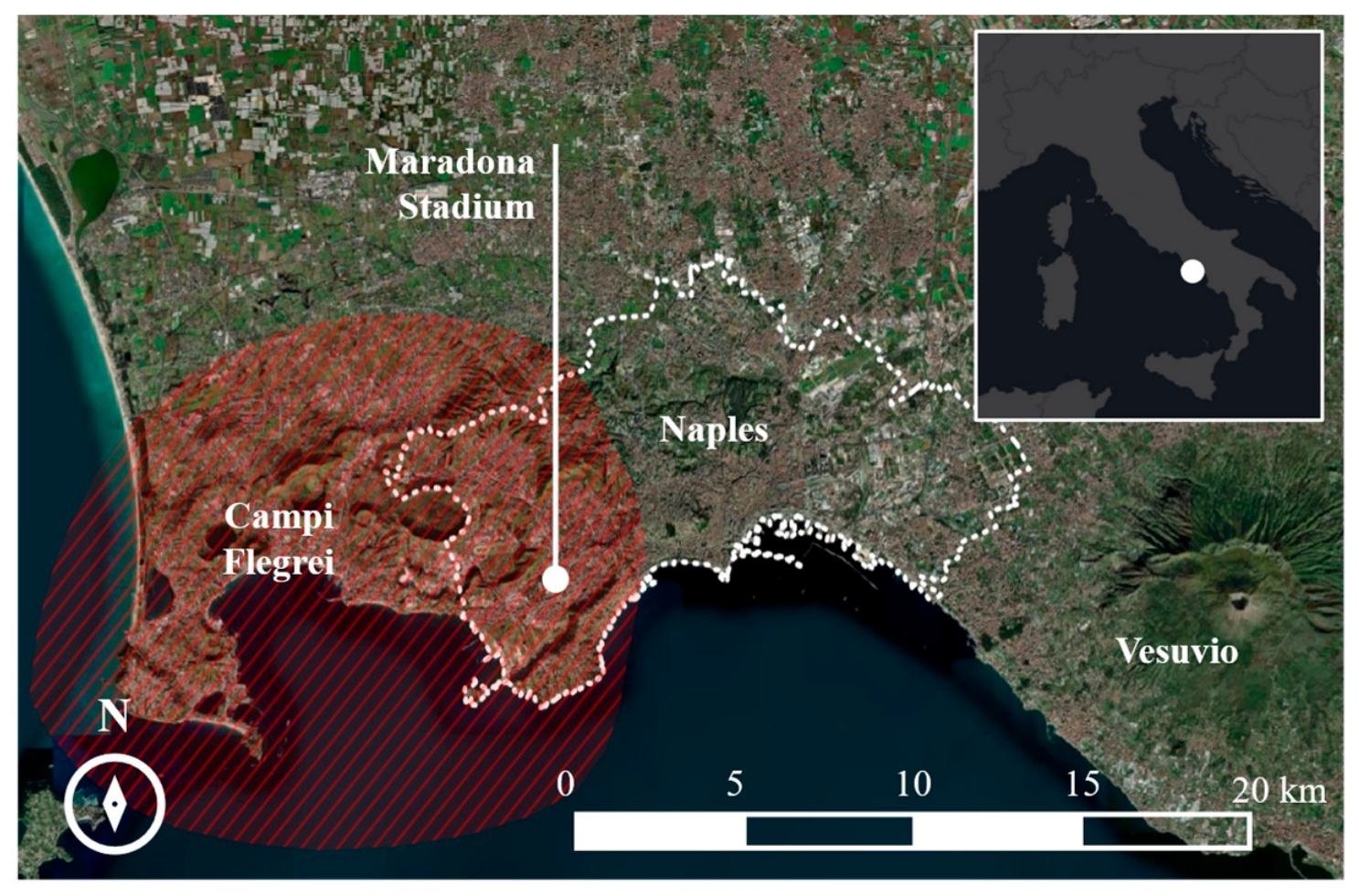
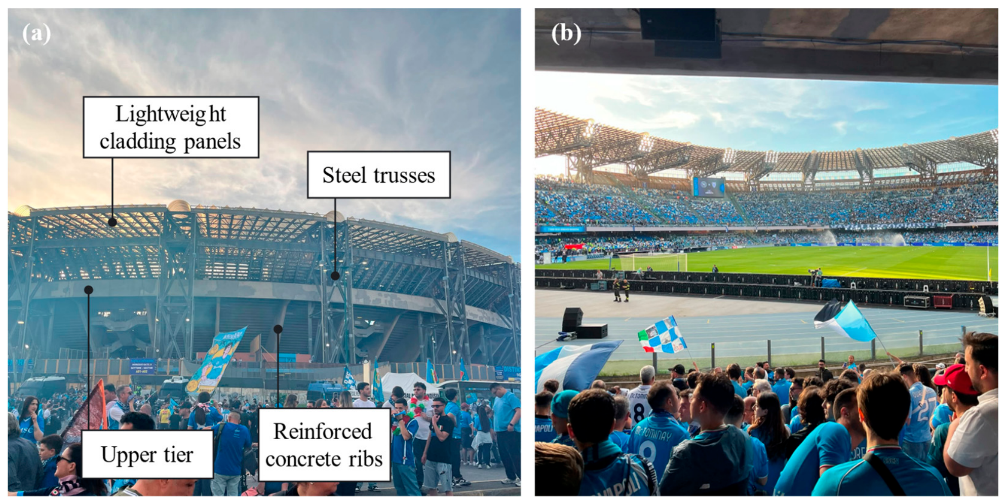
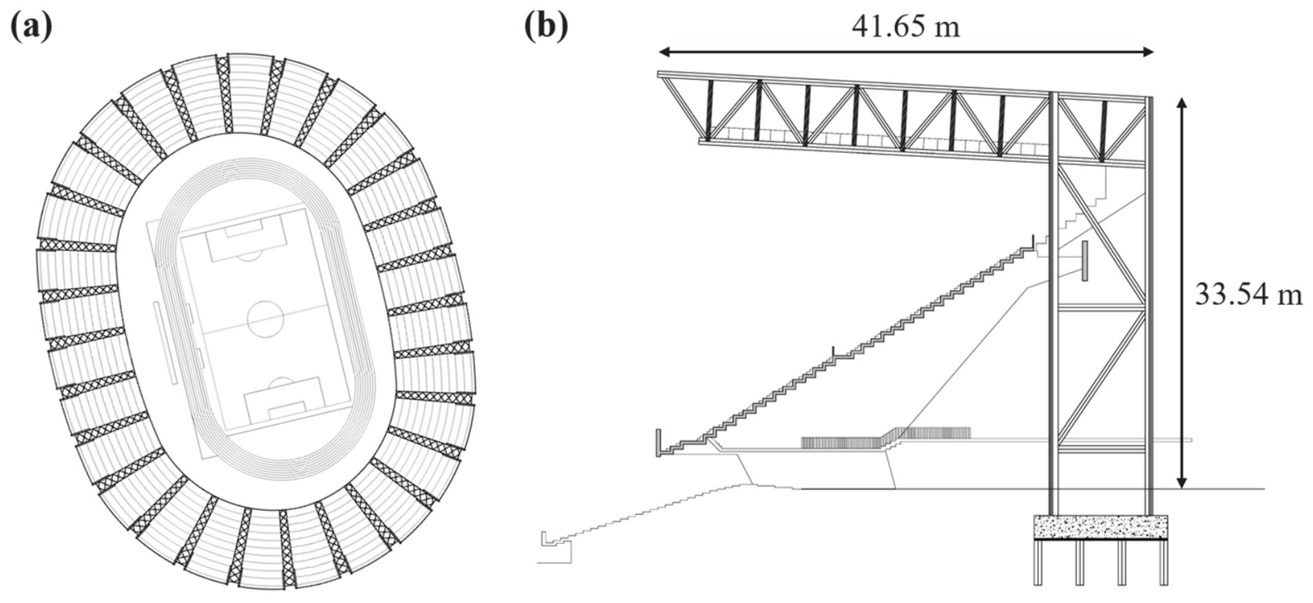
The goal of this paper is to investigate the use of InSAR time series for monitoring the displacement behaviour of a large civil structure located in an area affected by ground deformation. Specifically, the study focuses on the roof structure of the Diego Armando Maradona Stadium in Naples, Italy. The case study is of particular interest for several reasons: (1) The stadium is in an urban area where ground deformation phenomena are known to occur, making the separation between structural and ground-related displacements a key issue. (2) The roof is a large-span steel structure with an elliptical plan configuration and long cantilevered elements, for which thermal actions are expected to induce non-negligible seasonal displacement variations. (3) The main roof elements have different orientations in plan, which allows the influence of the relative geometry between structural elements and satellite acquisitions to be examined on a single structure.

The main contributions of this paper can be summarised as follows:

• It assesses the effect of large-scale ground deformation on the interpretation of InSAR measurements and quantifies the residual structural response once this component is removed.
• It quantifies how the geometry of ascending and descending acquisitions affects the reconstructed displacements of differently oriented roof trusses, showing how the projection of the actual structural displacement along the LOS varies with the in-plane orientation of the element, and it derives the error affecting the reconstructed components as a function of that orientation.
• It compares two strategies for the estimation and removal of the ground-motion component and discusses the effect of limited PS availability on the reliability of the computation.

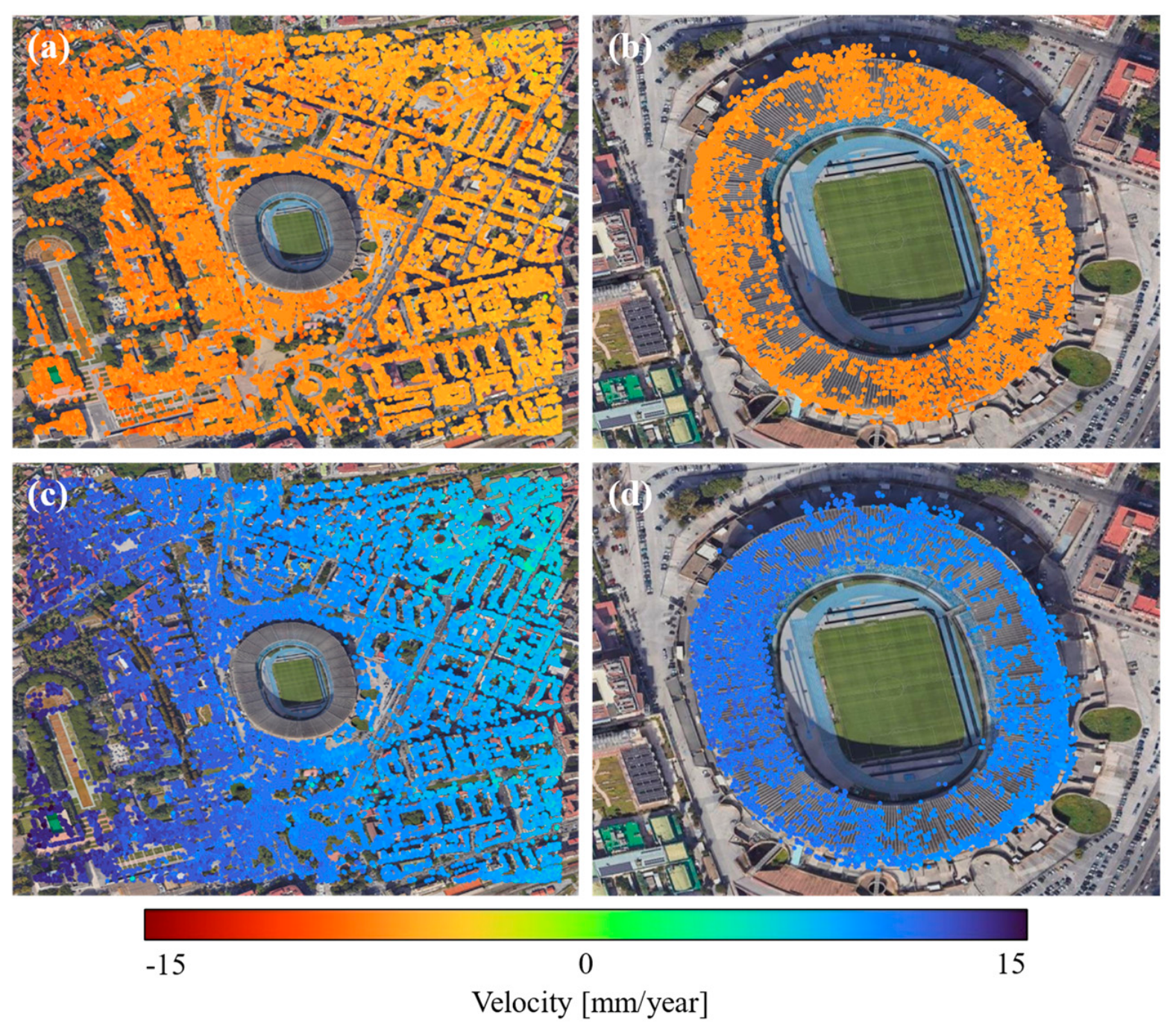
The InSAR data used in this study consist of COSMO-SkyMed displacement time series processed by CNR-IREA over the Naples metropolitan area. The availability of high-resolution X-band SAR data makes it possible to identify a dense set of PSs on the stadium roof and in the nearby urban environment, allowing both the local displacement response of the roof structure and the ground deformation affecting the area to be analysed. In this study, the InSAR time series are first used to characterise the deformation field in the surroundings of the stadium. Then, two strategies are adopted to estimate and compensate for the ground-motion component affecting the measured displacements on the roof. The resulting residual time series are finally analysed to study the behaviour of different zones of the roof.

The paper is organised as follows. Section 2 presents the methodology for InSAR displacement reconstruction and for the estimation and removal of the ground-deformation component. Section 3 describes the study area, the stadium, and the InSAR datasets. Section 4 presents and discusses the results, focusing on the interpretation of the reconstructed displacements. Finally, Section 5 summarises the main findings, discusses the limitations of the study, and outlines future developments for the use of InSAR in the monitoring of civil structures located in deforming urban areas.

2. InSAR Data Processing and Displacement Reconstruction

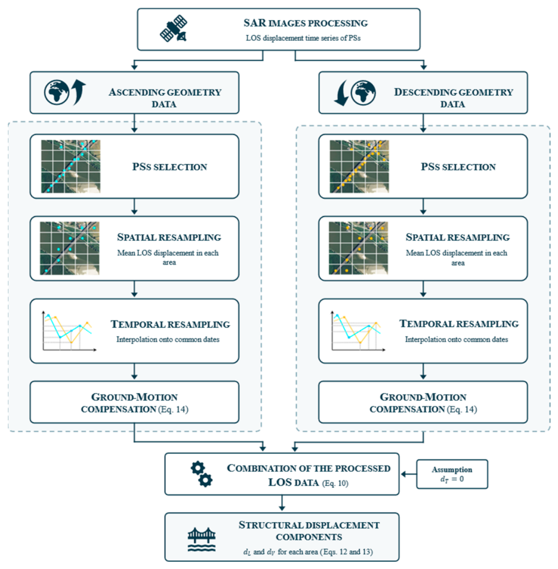
This section describes the procedure adopted to derive displacement time series from InSAR observations and to express them in a local structural reference system. The relationship between LOS measurements and structural displacement components is first introduced. The spatial and temporal resampling approaches required to combine independently processed ascending and descending datasets are then presented. Finally, the strategies adopted to model and remove the ground-deformation component are presented. The overall workflow, from the raw InSAR datasets to the reconstructed displacement components, is summarised in Figure 1.

The proposed framework provides a general methodology for separating regional ground deformation from structural response in InSAR-based monitoring of civil structures located in deforming environments.

2.1. Relationship Between LOS Observations and Structural Displacement Components

For a given PS on a structure, the displacement vector can be expressed in the East–North–Up (ENU) reference frame as:

$$\mathbf{d}=\left[\begin{array}{c}{d}_E\\ d_N\\ d_U\end{array}\right]$$

(1)

where d_E, d_N, and d_U are the displacement components along the East, North, and Up directions, respectively, at time t. The structural displacements refer to a generic acquisition epoch. Their dependence on time is therefore implicit and omitted from the notation for clarity.

The LOS displacement measured by acquisition i is the projection of d onto the SAR unit look-vector u_i. In this study, i ∈ {A,D}, where A denotes an ascending acquisition and D denotes a descending acquisition. The SAR unit look-vector is defined as:

$${\mathbf{u}}_i=\left[\begin{array}{c}\mathit{sin}{\theta }_i\mathit{cos}{\alpha }_i\\ -\mathit{sin}{\theta }_i\mathit{sin}{\alpha }_i\\ \cos {\theta }_i\end{array}\right]$$

(2)

where θ_i is the incidence angle measured from the vertical direction, and α_i is the look-azimuth angle measured clockwise from the East axis. Positive LOS displacement corresponds to motion toward the satellite. The LOS displacement is therefore written as:

$$d_{\mathrm{LOS},i}={\mathbf{u}}_i^{\mathrm{T}}\mathbf{d}=\sin {\theta }_i\left[\cos {\alpha }_i\hspace{0.17em}{d}_E-\sin {\alpha }_i\hspace{0.17em}{d}_N\right]+\cos {\theta }_i\hspace{0.17em}{d}_U$$

(3)

To facilitate the interpretation of structural displacements, a local reference system is introduced. This system is defined by the longitudinal direction L, the transverse direction T, and the vertical direction V. The longitudinal direction is aligned with the main axis of the considered structural element, the transverse direction is orthogonal to it in the horizontal plane, and the vertical direction coincides with the Up direction. The local displacement vector is

$${\mathbf{d}}_{\mathit{LTV}}=\left[\begin{array}{c}{d}_L\\ d_T\\ d_V\end{array}\right]$$

(4)

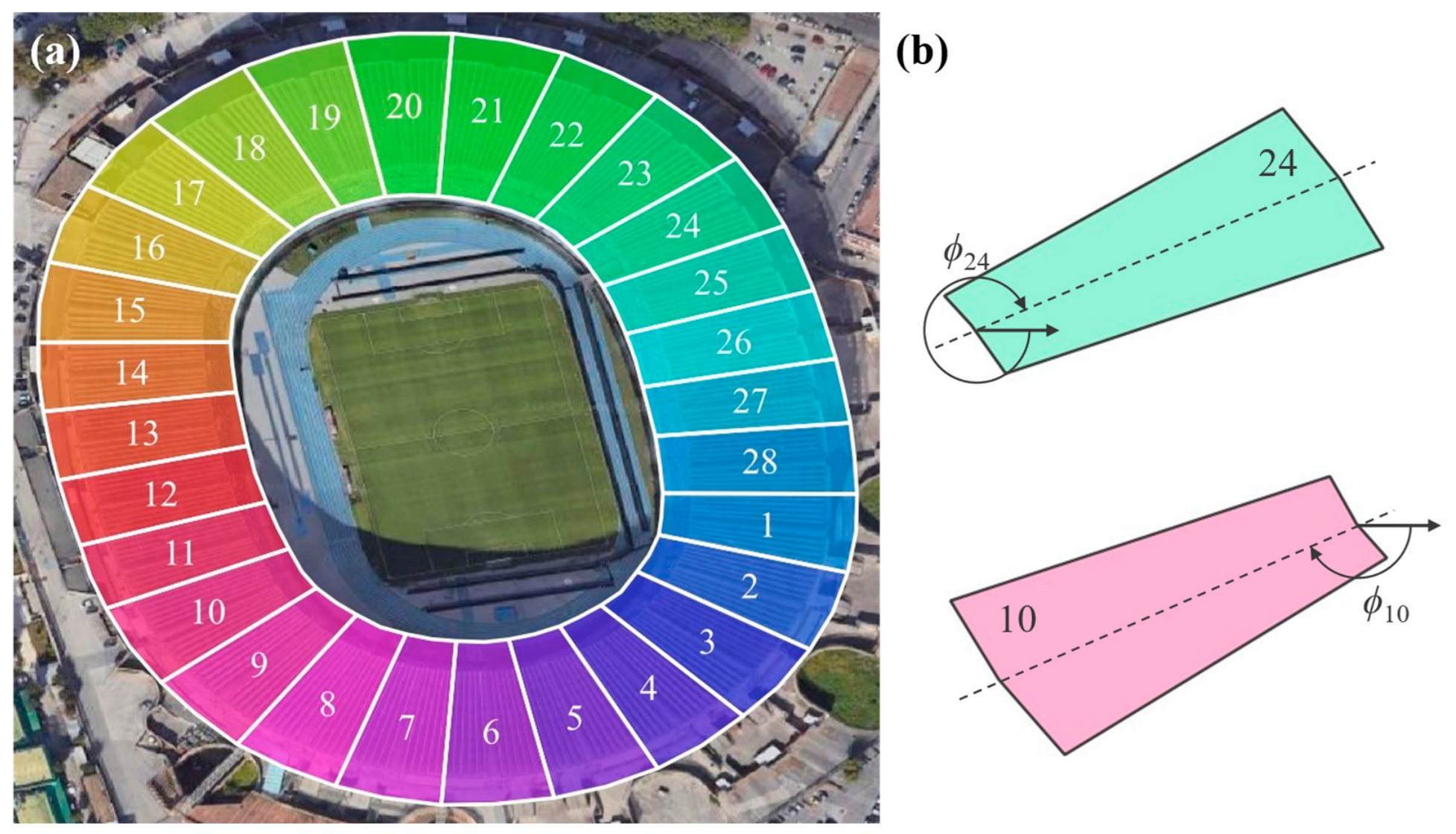
Let ϕ be the clockwise angle between the longitudinal axis and the East direction, measured with the same convention adopted for the look azimuth angle. The LOS displacement can be expressed directly in the local structural reference system as

d_LOS,i = sinθ_i[cos(α_i − ϕ)d_L − sin(α_i − ϕ)d_T] + cosθ_id_V

(5)

For compactness, the following geometric coefficients are introduced:

a_i = sinθ_icos(α_i − ϕ)

(6)

c_i = −sinθ_isin(α_i − ϕ)

(7)

b_i = cosθ_i

(8)

Using these coefficients, Equation (5) becomes:

d_LOS,i = a_id_L + c_id_T + b_id_V

(9)

When measurements from both ascending and descending acquisitions are available, the following system can be written:

$$\left\{\begin{array}{c}{d}_{\mathrm{LOS},A}=a_A{d}_L+c_A{d}_T+b_A{d}_V\\ d_{\mathrm{LOS},D}=a_D{d}_L+c_D{d}_T+b_D{d}_V\end{array}\right.$$

(10)

The system contains two equations and three unknown displacement components. Therefore, an additional assumption is required to obtain a unique solution. In the standard approach, the transverse displacement is assumed to be negligible, i.e., d_T = 0. Under this assumption, Equation (10) reduces to:

$$\left\{\begin{array}{c}{d}_{\mathrm{LOS},A}=a_A{d}_L+b_A{d}_V\\ d_{\mathrm{LOS},D}=a_D{d}_L+b_D{d}_V\end{array}\right.$$

(11)

Solving Equation (11), the longitudinal and vertical displacement components are obtained as

$$d_L={\displaystyle \frac{b_D{d}_{\mathrm{LOS},A}-b_A{d}_{\mathrm{LOS},D}}{a_A{b}_D-a_D{b}_A}}$$

(12)

$$d_V={\displaystyle \frac{a_A{d}_{\mathrm{LOS},D}-a_D{d}_{\mathrm{LOS},A}}{a_A{b}_D-a_D{b}_A}}$$

(13)

The coefficients a_A, a_D, b_A, and b_D depend on the satellite acquisition geometries and on the orientation ϕ of the structural element. For a given structural element and fixed acquisition geometries, these coefficients can be considered constant in time. If different structural elements have different orientations, the coefficients are computed separately for each element or analysed area.

Ascending and descending acquisitions are processed independently and therefore provide PSs at different spatial locations and acquisition dates. The spatial mismatch between the PSs arises because PS identification is performed independently for each image stack, retaining only those targets that exhibit stable scattering properties throughout the corresponding set of acquisitions: each identified PS is associated with a fixed spatial position and a single displacement time series. Differences in acquisition dates, instead, reflect the satellite revisit cycle, with consecutive acquisitions typically separated by several days. To make the two datasets spatially comparable, a grid subsampling approach is adopted. The investigated structure is divided into analysis areas or structural zones, and each zone is assigned representative LOS displacement time series derived from the PSs located within it. Temporal consistency is then achieved through linear interpolation of each dataset at the acquisition dates of the other. This provides paired ascending and descending measurements at every acquisition date of either orbit. Further details on grid subsampling, linear temporal interpolation, and their implications for InSAR-based structural displacement reconstruction are reported in previous studies [11,26].

2.2. Modelling and Removal of Ground Deformation

The LOS displacement measured on a structure may include both the local structural response and the contribution of ground deformation affecting the surrounding area. The structural component includes the mechanical response of the structure and the effects of operational and environmental actions, such as temperature-induced variations. The ground-related component accounts for broader deformation processes occurring at the scale of the surrounding area.

For each acquisition geometry i and considered area, at a given acquisition time, the observed LOS displacement is decomposed as

$$d_{\mathrm{LOS},i}=d_{\mathrm{LOS},i}^{\mathrm{str}}+d_{\mathrm{LOS},i}^{\mathrm{gr}}$$

(14)

where $d_{\mathrm{LOS},i}^{\mathrm{str}}$ is the component associated with the local structural response, and $d_{\mathrm{LOS},i}^{\hspace{0.17em}\mathrm{gr}}$ is the component associated with ground deformation. The objective of the compensation procedure is to estimate the ground-related component and subtract it from the observed LOS displacement.

The first strategy consists of estimating the ground-deformation contribution from a set of reference PSs located in the surroundings of the structure, similarly to what has been done in previous studies [32,34]. For each acquisition geometry, the ground-related component is computed as the mean LOS displacement of the selected reference PSs. This approach assumes that the reference PSs undergo the same ground movement affecting the investigated structure, and that this ground motion is the dominant contribution to their displacement. Their mean displacement is therefore interpreted as a rigid or quasi-rigid motion of the surrounding ground, common to both the reference area and the structure. This strategy is appropriate when the deformation field is relatively uniform over the area considered and the reference PSs are sufficiently close to the structure to experience comparable ground motion.

The second strategy also relies on reference PSs located in the surroundings of the structure, but it estimates the ground-deformation component by fitting their displacement time histories with an analytical function, such as a polynomial. In this case, the fitted curve is interpreted as the temporal evolution of the ground movement. The underlying assumption is that the ground-related component evolves smoothly over time, so that short-term fluctuations or local deviations observed at individual PSs may be associated with measurement variability, local effects, or non-representative behaviour. The analytical fitting therefore acts as a temporal regularisation of the reference PS information and extracts the dominant long-term trend associated with the ground deformation process. In this study, the ground-deformation component is modelled as a second-order polynomial in time:

$$d_{\mathrm{LOS},i}^{\mathrm{gr}}=a_{2,i}{\left(t-t_0\right)}^2+a_{1,i}\left(t-t_0\right)+a_{0,i}$$

(15)

where t₀ is the first acquisition date, a_0,i is the mean LOS displacement of the reference PSs at t₀, and a_1,i and a_2,i are estimated by least-squares regression. The regression is performed on the displacement time series of the individual reference PSs taken jointly, so that each PS contributes through the epochs at which a valid measurement is available. Anchoring the curve to the reference PS displacement at the beginning of the monitoring period prevents offsets between the mean-reference and polynomial corrections, while the quadratic term accounts for the curvature of the long-term deformation trend.

After removing the ground-related component from the ascending and descending LOS displacement time series, the structural displacement components are estimated using Equations (12) and (13), following the spatial and temporal resampling operations described above.

2.3. Conditioning of the Reconstruction and Error of the Estimated Displacements

As shown in Equations (12) and (13), the reconstruction of d_L and d_V involves the common denominator (a_Ab_D − a_Db_A), which depends on the two satellite acquisition geometries and on the orientation of the structural element; denoting by H the coefficient matrix of the linear system in Equation (11), this denominator corresponds to det(H), i.e., det(H) = a_Ab_D − a_Db_A. When it approaches zero, meaning that the longitudinal axis of the element is nearly aligned with the satellite along-track direction, the two LOS equations become nearly singular, and small perturbations in the input LOS time series are strongly amplified in the reconstructed displacement components. The condition number κ(H) provides a complementary measure of the sensitivity of the reconstruction to perturbations in the LOS data [37]. Here, κ(H) is taken as the ratio between the largest and smallest singular values of H:

$$\kappa \left(\mathbf{H}\right)={\displaystyle \frac{{\sigma }_{\max }\left(\mathbf{H}\right)}{{\sigma }_{\min }\left(\mathbf{H}\right)}}$$

(16)

Values of κ(H) close to unity indicate a well-conditioned system, whereas large values indicate an ill-conditioned reconstruction, in which small LOS measurement errors may be strongly amplified in the estimated displacement components.

The reconstructed displacement components are affected by two types of error: systematic and random [25]. The first originates from the assumption introduced to make the system determined: if the transverse displacement d_T is not exactly null, the component neglected in the reconstruction is redistributed over the two estimated ones, producing a deviation from their actual values. The second originates from the LOS measurements themselves, whose dispersion propagates through the inversion and affects the estimates in a random manner.

The systematic error is obtained by substituting Equation (10), in which d_T is retained, into Equations (12) and (13), which are derived under the assumption d_T(t) = 0. The estimated components then differ from the actual ones by the following bias terms:

$$e_{b,L}={\displaystyle \frac{b_D{c}_A-b_A{c}_D}{a_A{b}_D-a_D{b}_A}}{d}_T,\hspace{1em}\hspace{1em}{e}_{b,V}={\displaystyle \frac{a_A{c}_D-a_D{c}_A}{a_A{b}_D-a_D{b}_A}}{d}_T$$

(17)

The systematic error depends linearly on the neglected transverse displacement component.

The random error is associated with the variability of the LOS measurements assigned to each area. For each acquisition geometry and acquisition time, the PSs grouped within the same area are treated as repeated measurements of the same underlying area-level LOS displacement [26]. Let d_LOS,i,n denote the displacement measured at the n-th PS for acquisition geometry i, and let N_i be the number of PSs within the area. The representative LOS displacement assigned to the area is obtained as the arithmetic mean of the PS measurements:

$$d_{\mathrm{LOS},i}={\displaystyle \frac{1}{N_i}}{\displaystyle \sum _{n=1}^{N_i}}{d}_{\mathrm{LOS},i,n}$$

(18)

The dispersion of the individual PS measurements around this representative value is quantified by the sample standard deviation:

$${\sigma }_{\mathit{LOS},i}=\sqrt{{\displaystyle \frac{1}{N_i-1}}{\displaystyle \sum _{n=1}^{N_i}}{\left(d_{\mathrm{LOS},i,n}-d_{\mathrm{LOS},i}\right)}^2}$$

(19)

The reconstructed components are linear combinations of the LOS observations, so that their covariance follows from the covariance of the observations. Assuming errors with zero mean and no correlation between the two acquisition geometries, which are processed independently, the covariance matrix of the estimated components is:

$$\mathbf{P}={\left({\mathbf{H}}^{\mathrm{T}}{\mathbf{R}}^{-1}\mathbf{H}\right)}^{-1}$$

(20)

where R is the covariance matrix of the LOS observations at the same epoch, whose diagonal terms are the variances of the ascending and descending measurements with zero off-diagonal terms because the two datasets are processed independently, i.e., $\mathbf{R}=\mathit{diag}\left({{\sigma }_A}^2,{{\sigma }_D}^2\right)$. The diagonal terms of P are the variances of the two reconstructed components. Carrying out the product, the variances of the two reconstructed components read:

$$P_{11}={\displaystyle \frac{b_D^2{\sigma }_A^2+b_A^2{\sigma }_D^2}{{\left(a_A{b}_D-a_D{b}_A\right)}^2}},\hspace{1em}\hspace{1em}{P}_{22}={\displaystyle \frac{a_D^2{\sigma }_A^2+a_A^2{\sigma }_D^2}{{\left(a_A{b}_D-a_D{b}_A\right)}^2}}$$

(21)

Thus, the standard deviations of the reconstructed longitudinal and vertical displacement read, respectively:

$$e_{r,L}=\sqrt{P_{11}},\hspace{1em}\hspace{1em}{e}_{r,V}=\sqrt{P_{22}}$$

(22)

The two contributions are finally combined into a single measure of the error affecting the estimated components, as follows:

e_L = |e_b,L| + e_r,L, e_V = |e_b,V| + e_r,V

(23)

Both contributions are inversely proportional to |det(H)|, so that an element whose orientation approaches a singular one is affected by a larger systematic and random errors. The conditioning of the reconstruction, introduced at the beginning of this section as a relative measure of the amplification, therefore governs both terms of Equation (23), linking the geometry of the acquisitions and the error affecting the estimated displacement components. It should be noted that both error contributions and thus the total error vary between acquisition epochs, although this dependence is not explicitly shown in the notation.

3. Study Area and Case Study

3.1. Regional Setting and Ground Deformation

The Naples metropolitan area lies in the central sector of the Campanian volcanic district, between the Campi Flegrei caldera to the west and the Somma-Vesuvio volcanic complex to the east (Figure 2). Campi Flegrei is an active nested caldera whose most distinctive geodynamic expression is bradyseism, namely slow and partly reversible ground deformation driven by pressure changes in the shallow subsurface. These pressure changes are associated with the accumulation and release of magmatic and hydrothermal fluids along pre-existing fractures. Over the past century, the caldera has alternated between prolonged subsidence phases and discrete unrest episodes. The most intense recent episodes occurred in 1969–1972 and 1982–1984, producing a cumulative uplift of approximately 3.5 m around Pozzuoli [38]. A renewed inflationary phase began in late 2005 and is ongoing [39]; by late 2023, the maximum vertical displacement had exceeded 110 cm since the start of the inflationary phase, accompanied by increased shallow seismicity and intensified hydrothermal manifestations [40]. The spatial extent of this deformation field encompasses the full caldera and extends into the broader Naples urban area, including the Fuorigrotta district where the Diego Armando Maradona Stadium is located.

3.2. The Diego Armando Maradona Stadium

The Diego Armando Maradona Stadium (40.8280° N, 14.1930° E) is a multipurpose facility, with a current seating capacity of approximately 55,000 spectators (Figure 3). Construction began in the early 1950s and the venue was inaugurated in 1959. It serves as the home ground of SSC Napoli and has hosted major international events, including the 1990 FIFA World Cup, which prompted a substantial structural refurbishment.

The original structural system is constructed of reinforced concrete and consists of a continuous bowl arranged in two tiers. The lower tier is founded directly on the ground, whereas the upper tier is supported by 56 large inclined reinforced concrete ribs, radially distributed and connected to the foundations. The refurbishment carried out for the 1990 FIFA World Cup added a third tier and the current roof system, consisting of a circumferential ring of steel trusses supporting lightweight cladding panels. The roof reaches an overall height of approximately 33.5 m, with truss cantilevers extending approximately 41.6 m inward from the supporting ring (Figure 4).

The Maradona Stadium represents a particularly suitable case study for demonstrating the proposed methodology for several reasons. First, its location within the Campi Flegrei caldera exposes the structure to significant regional ground deformation, making the separation between structural and ground-related displacements a fundamental challenge. Second, the large steel roof provides numerous coherent PSs, enabling a dense spatial sampling of the structural response over a long observation period. Third, the radial arrangement of the roof trusses, which span a wide range of orientations with respect to the satellite acquisition geometries, offers the opportunity to investigate how structural orientation affects the conditioning of the displacement reconstruction problem. Finally, the lightweight steel cantilever roof is expected to exhibit measurable thermally induced deformations, providing a physically meaningful benchmark for assessing whether the corrected InSAR measurements successfully isolate the actual structural response from the regional ground motion. The roof structure of the stadium is the primary subject of this study. In plan, it follows the elliptical geometry of the stadium, with 28 similar radial steel trusses distributed around the perimeter. Each truss is oriented differently with respect to a fixed reference direction. The orientation angle ϕ_k, with k = 1, …, 28, defined as the clockwise rotation from the East direction to the truss longitudinal axis, varies continuously around the perimeter and spans the full 360° range across the 28 trusses. For the analysis, the roof ring was discretised into 28 areas, numbered clockwise, each corresponding to one radial truss, as shown in Figure 5. The orientation angle associated with each area is reported in

Table 1. Orientation angle ϕ_k for each of the 28 roof areas.

Area	ϕk [°]	Area	ϕk [°]	Area	ϕk [°]
1	4.20	11	165.25	21	286.62
2	17.39	12	168.22	22	306.31
3	31.00	13	171.97	23	322.75
4	46.70	14	176.17	24	338.32
5	64.82	15	183.34	25	344.97
6	86.72	16	196.44	26	349.30
7	106.63	17	209.96	27	353.13
8	124.88	18	225.97	28	357.48
9	142.10	19	245.26
10	156.63	20	266.32

.

3.3. InSAR Datasets

The interferometric products used in this study were generated by CNR-IREA through the Parallel SBAS processing chain, starting from COSMO-SkyMed images acquired in Stripmap mode. The ascending dataset spans July 2009 to March 2025 and includes 432 acquisition dates, whereas the descending dataset spans July 2011 to March 2025 and includes 213 acquisition dates; the analysis was carried out over the observation period common to the two geometries. The processing was carried out using the SRTM 1 arcsec DEM in the WGS84 geographic reference system (EPSG:4326). The ascending acquisitions are characterised by an incidence angle θ_A = 49.25° and an azimuth angle α_A = 171.61°, while the corresponding values for the descending acquisitions are θ_D = 25.53° and α_D = 11.00°, respectively.

From the full track footprints, a 1 km² area centred on the stadium was extracted for the analysis. Within this area, PSs located on the stadium were separated from those in the surrounding urban area on the basis of their planimetric position alone, using the software QGIS 3.36.0. All the subsequent operations described in Section 2, from the spatial and temporal resampling of the two datasets to the estimation and removal of the ground-deformation component and to the reconstruction of the displacement components, were implemented by the authors in MATLAB R2023b.

The surrounding area, obtained by removing the stadium footprint from the square, covers around 938,000 m² and contains 56,198 ascending and 57,734 descending PSs, corresponding to densities of 0.060 and 0.062 PS/m². The 28 roof areas cover roughly 42,000 m², with a mean surface of about 1,500 m² per area, and contain 7,826 ascending and 8,262 descending PSs, that is 0.185 and 0.195 PS/m². The number of PSs available in a single roof area ranges from 160 to 381 in the ascending dataset and from 132 to 563 in the descending one. Figure 6 shows the spatial distribution of the PSs around the stadium for the ascending (a,b) and descending (c,d) tracks. Negative velocities, shown in red, indicate motion away from the satellite, whereas positive velocities, shown in blue, indicate motion toward it.

4. Results and Discussion

This section presents the results of the InSAR-based analysis of the stadium roof. First, the displacement components are reconstructed using the classical InSAR approach, without removing the ground-deformation component. Second, the two compensation strategies introduced in Section 2.2 are applied and compared, both in the LOS domain and in terms of reconstructed structural displacement components. Finally, the selection of reference PSs is refined by restricting the reference population to ground PSs located immediately adjacent to each roof area.

4.1. Displacement Reconstruction Without Ground-Deformation Correction

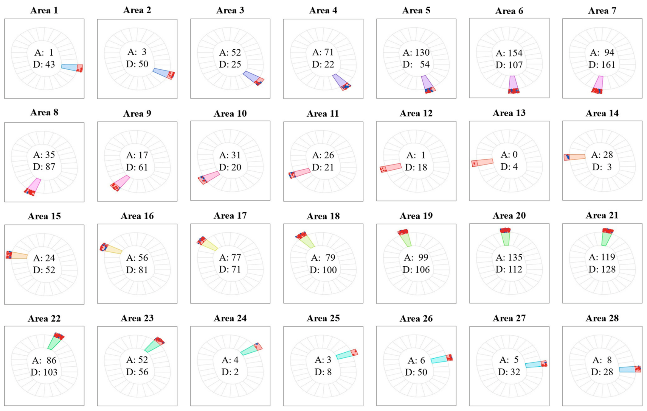
The displacement reconstruction was first carried out by combining ascending and descending LOS measurements without applying any correction for the ground-deformation component. Throughout the remainder of this paper, the same colour scheme as in Figure 5a is used to identify the 28 areas in all displacement time series.

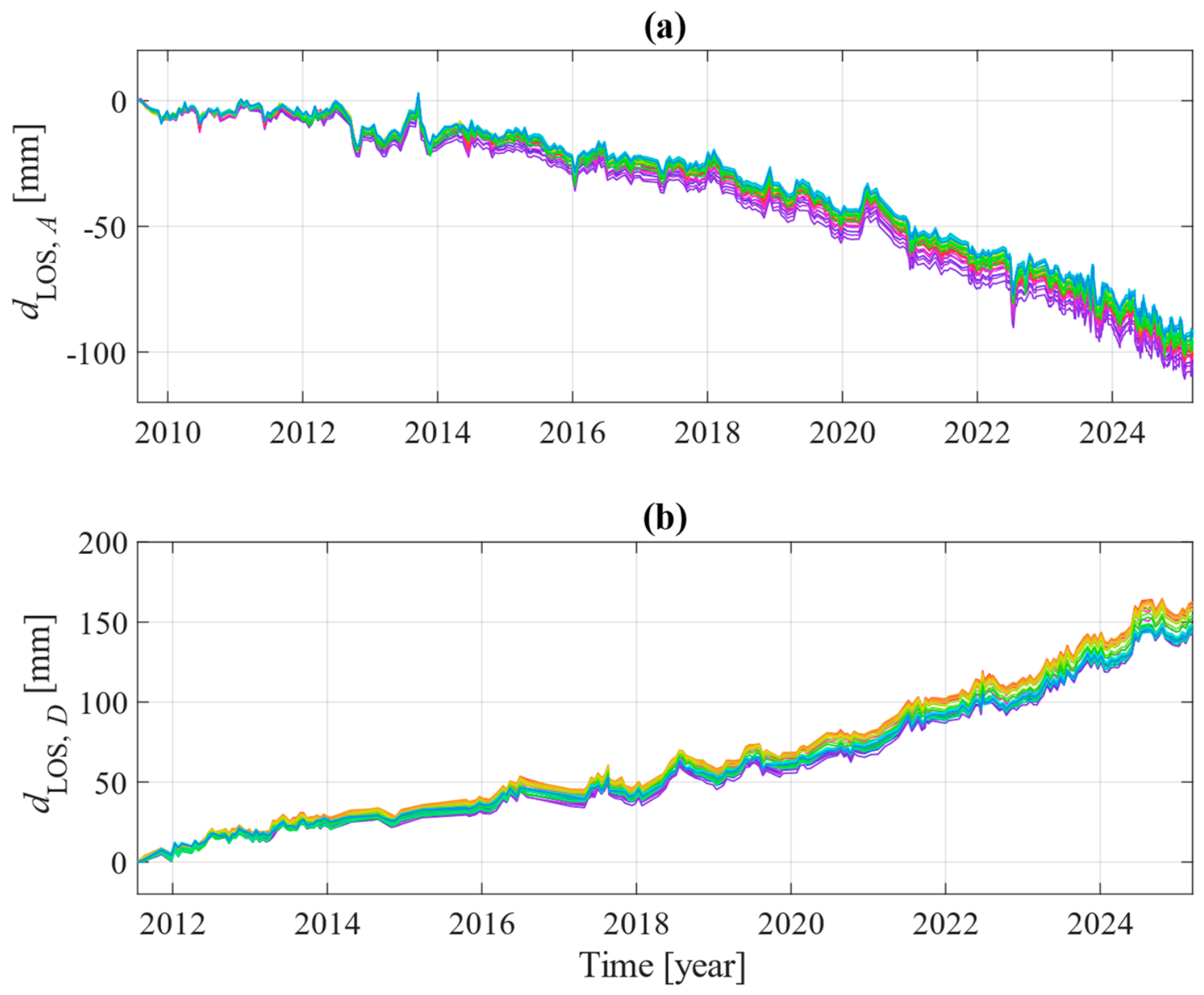
Figure 7 shows the LOS mean displacement time series measured on the 28 roof areas for the ascending and descending acquisition geometries. In both cases, the time series exhibit a pronounced common trend across all areas. In the ascending geometry, the cumulative LOS variation over the monitoring period is approximately −100 mm, whereas in the descending geometry it exceeds 150 mm. The opposite signs observed in the two acquisition geometries indicate that the dominant LOS signal includes a horizontal component [37]. A purely vertical displacement would produce LOS time series of the same sign in both geometries, because the vertical sensitivity of ascending and descending acquisitions has the same polarity. This behaviour is consistent with the known deformation pattern of Campi Flegrei, where caldera inflation produces both vertical uplift and horizontal motion [39,41].

The uncorrected ascending and descending LOS time series were then combined to reconstruct the longitudinal and vertical displacement components in the local reference system of each steel truss, under the assumption that the transverse displacement component is null, as defined in Section 2. This assumption is not strictly valid for the uncorrected signal, because the lateral ground motion projects onto each local transverse axis; the reconstruction is nevertheless carried out to illustrate how ground deformation propagates into the reconstructed displacements when it is not compensated. 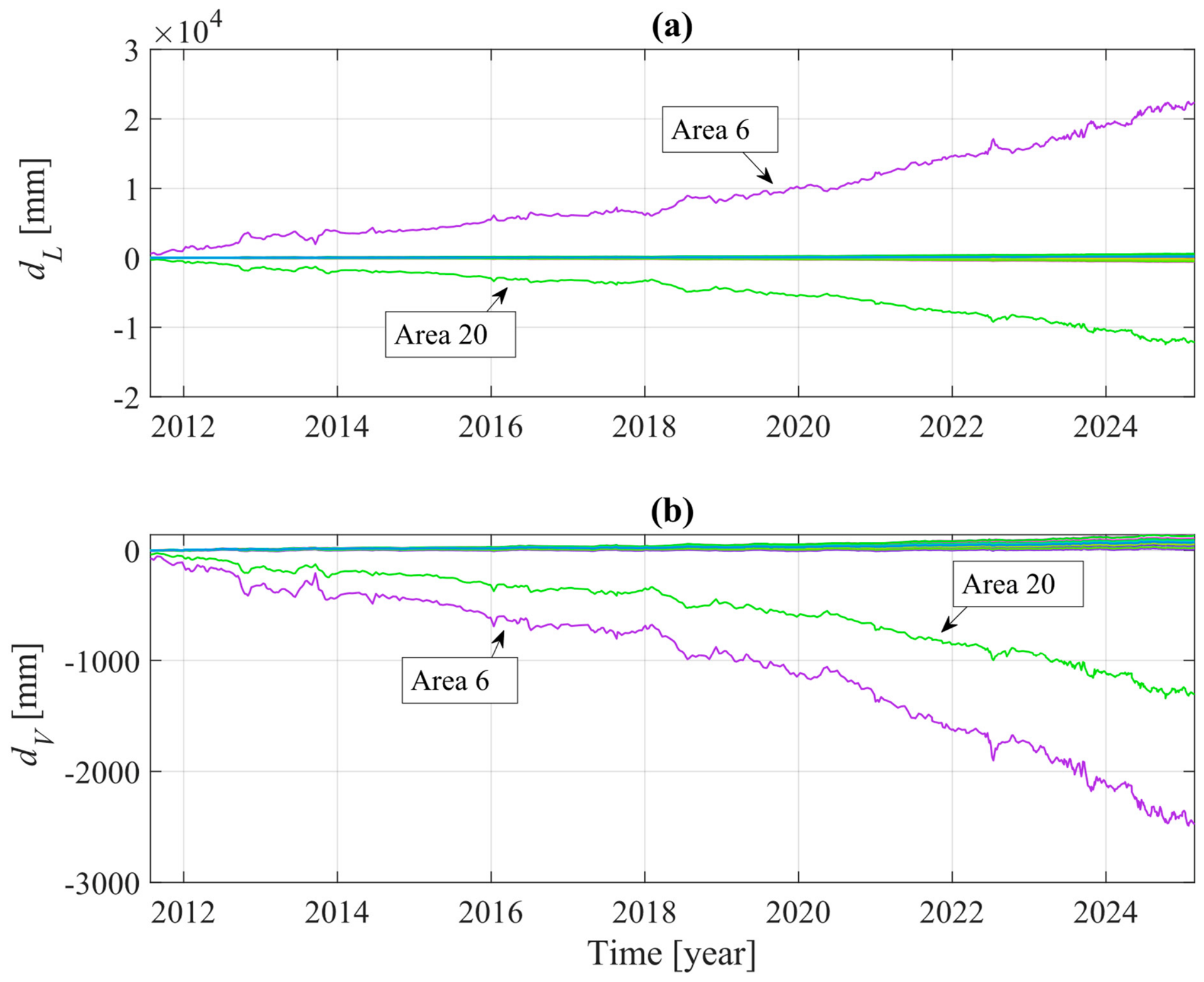Figure 8 shows the longitudinal and vertical displacement components reconstructed for the 28 roof areas. For both components, two time series show anomalously large amplitudes compared with the others. Since no major anomalies are exhibited by any part of the roof, this trend suggests an ill-conditioned reconstruction for the associated roof areas.

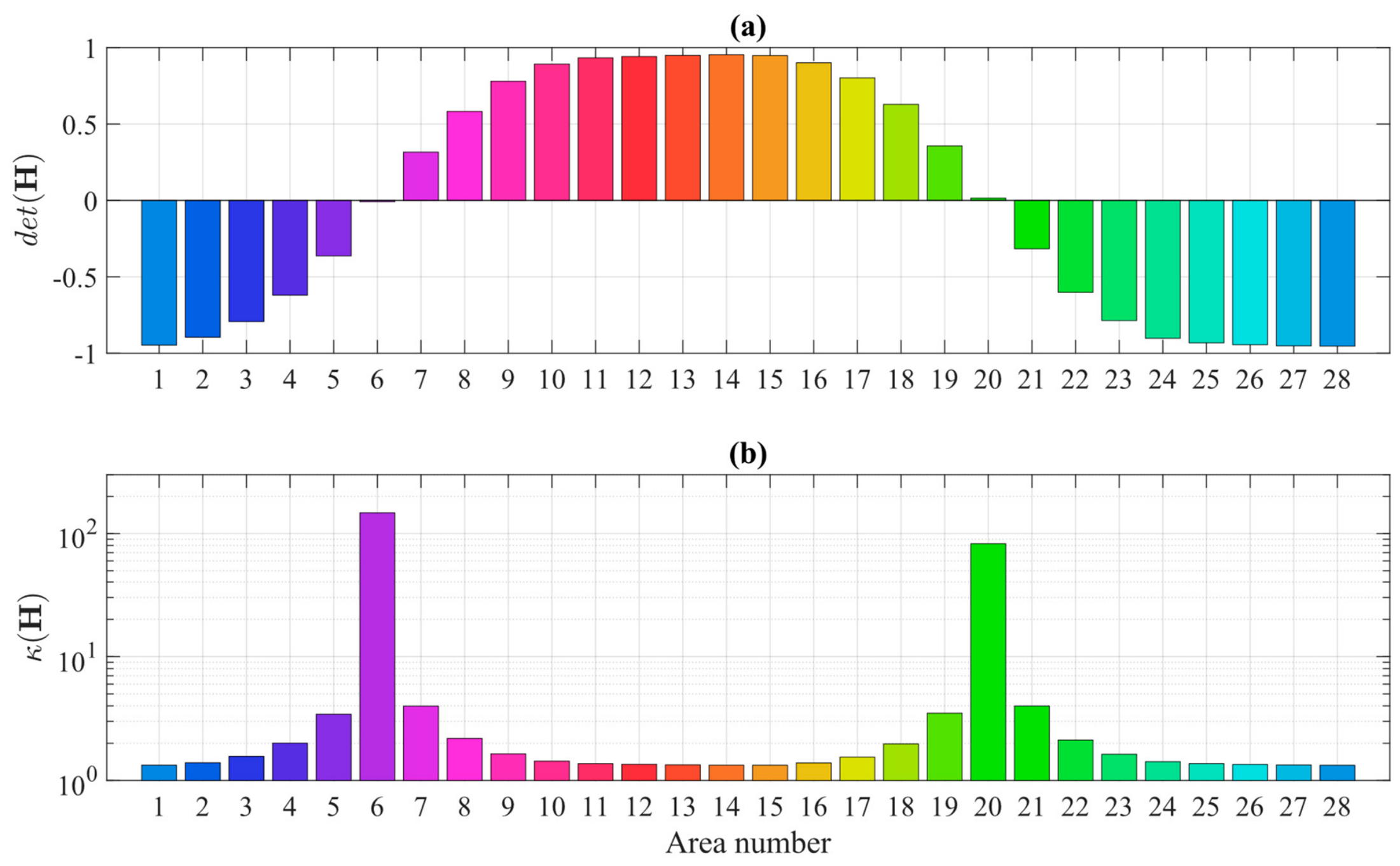
Figure 9 shows det(H) and κ(H) for the 28 roof areas, computed as described in Section 2.3. The determinant is zero for ϕ = 87.2° and ϕ = 267.2°, that is, when the longitudinal axis of the truss approaches the satellite along-track direction and the two LOS equations no longer carry independent information on d_L. Areas 6 and 20, whose orientations lie 0.5° and 0.9° from these directions, have |det(H)| equal to 0.009 and 0.015 and κ(H) of 147 and 83. All the remaining areas have κ(H) below 4.0, the minimum being 1.33 for the areas whose longitudinal axis is closest to the East–West direction.

The condition number expresses the amplification in relative terms, indicating by what factor a perturbation of the LOS measurement is amplified in the reconstructed components, irrespective of its magnitude. Areas 6 and 20 differ from the remaining roof areas by more than one order of magnitude in κ(H) and are therefore excluded from the quantitative interpretation, with the analysis proceeding on the remaining 26 areas. Their exclusion reflects the geometric observability limit discussed in Section 2.3: the longitudinal axes of these trusses lie close to the satellite along-track direction, so that neither the ascending nor the descending LOS carries independent information on d_L, and the reconstruction becomes ill-posed regardless of the quality of the LOS measurements.

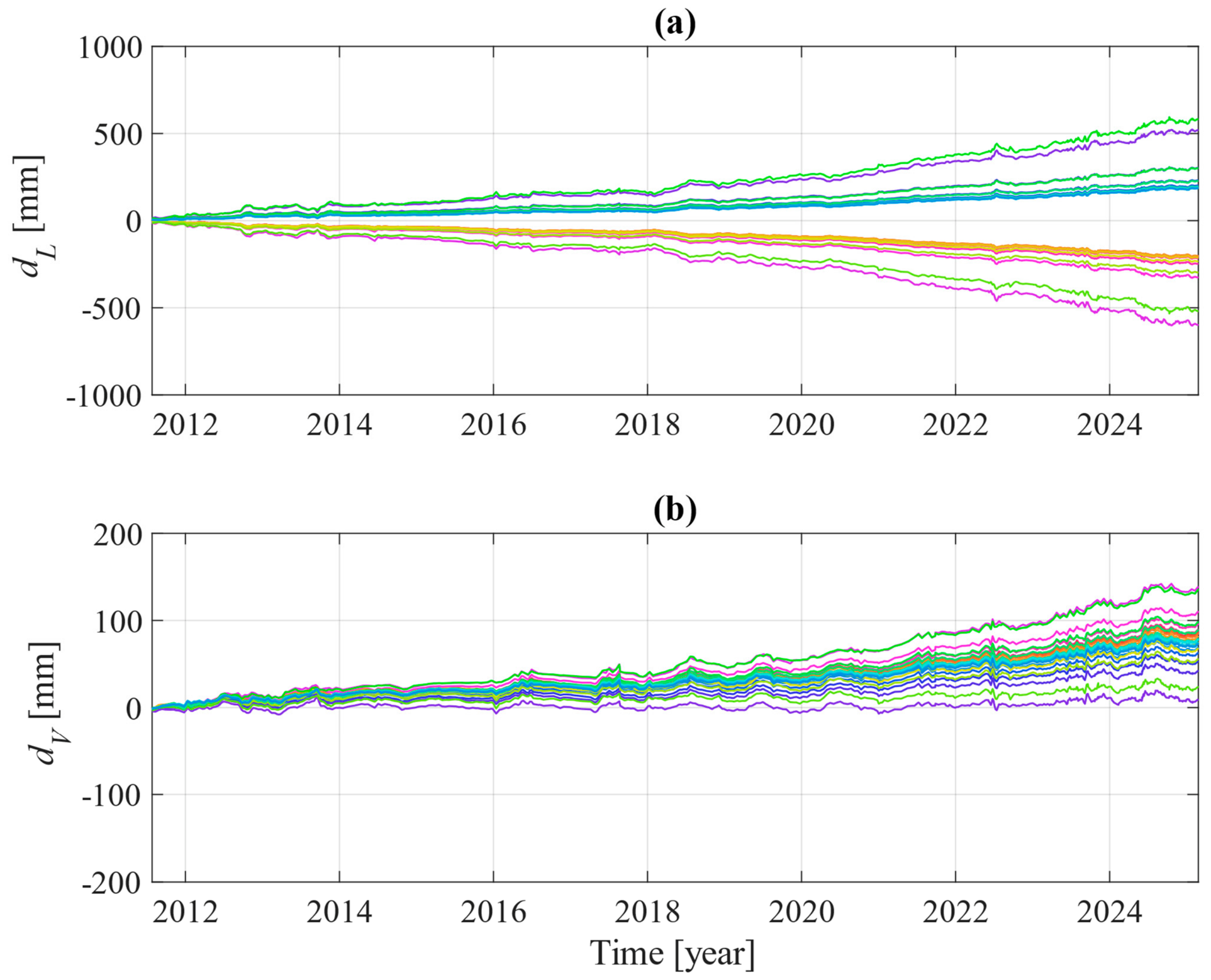
Figure 10 shows the reconstructed d_L and d_V for the 26 retained areas. The longitudinal component shows opposite signs in different sectors of the roof. This result is mainly related to the definition of the local reference system. The longitudinal component is positive when the displacement is directed along the positive longitudinal axis of the corresponding truss, and negative when it is directed in the opposite direction. Since the radial trusses have different orientations along the elliptical perimeter, the same horizontal displacement of the stadium area is projected with different signs onto the local longitudinal axes. In particular, a nearly eastward displacement gives positive values of d_L for trusses whose local longitudinal axis has an eastward component, and negative values for trusses whose local longitudinal axis has a westward component. The observed behaviour is consistent with a nearly uniform eastward rigid translation of the stadium area. The sign changes between areas 6 and 7 and between areas 20 and 21, around the two orientations coinciding with the singular directions identified above.

The vertical displacement component exhibits a general upward trend, reaching at the end of the observation period a mean value of 78 mm over the retained areas, with values ranging from 10 to 139 mm, in agreement with the ongoing ground uplift affecting the Fuorigrotta district.

The ground-motion component dominates the reconstructed longitudinal and vertical displacements and prevents direct interpretation of the behaviour of the roof structure. Furthermore, before removal of the ground-deformation component, the assumption of negligible transverse displacement is not generally satisfied, because the measured displacement field includes lateral ground movements associated with the broader deformation of the area. These results confirm that the ground-deformation component must be estimated and removed from the LOS measurements before the residual displacement time series can be interpreted as representative of the roof response.

4.2. Ground-Deformation Compensation and Displacement Reconstruction

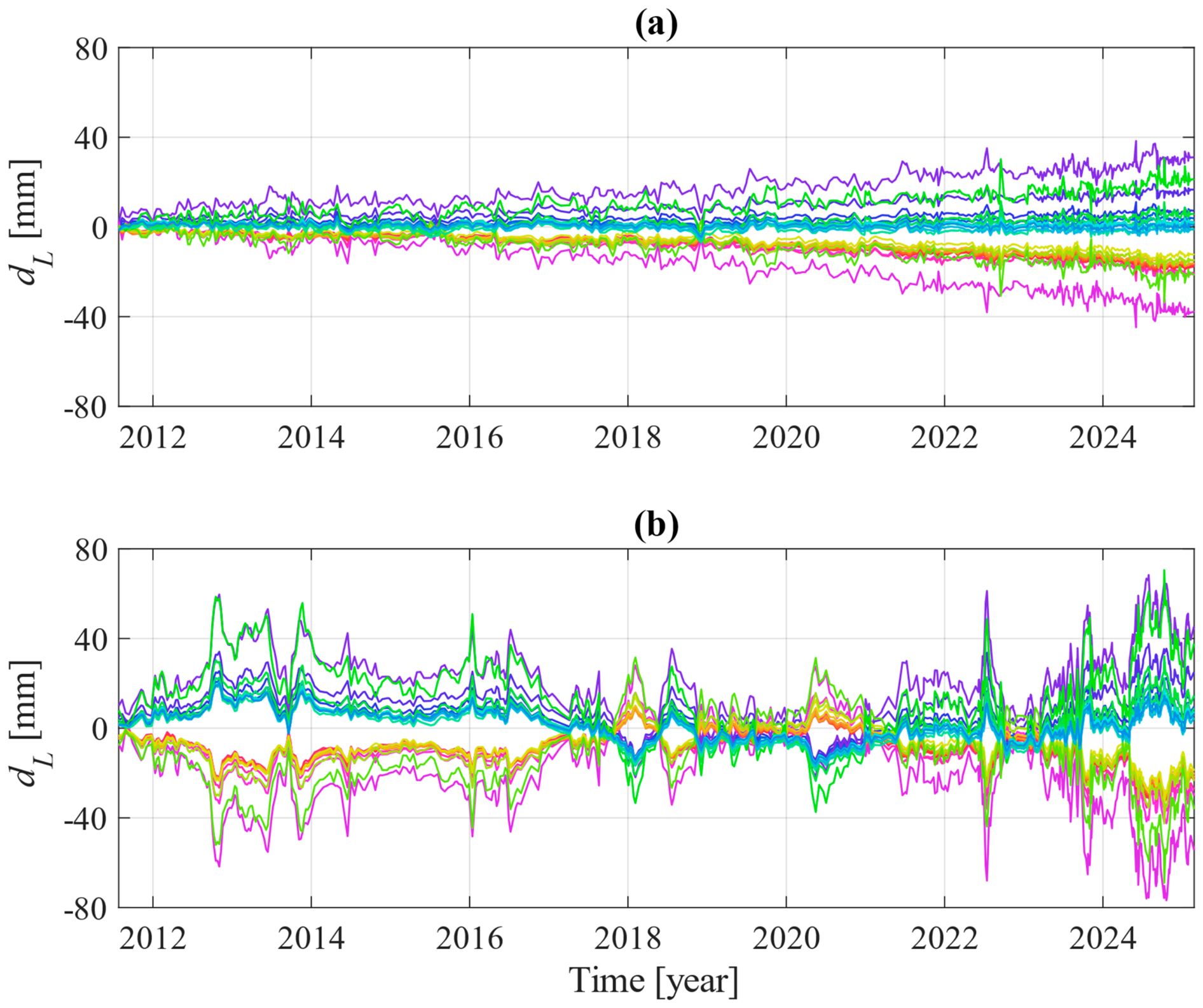
The two correction strategies described in Section 2.2 were applied independently to the ascending and descending LOS datasets. The corrected LOS time series were then combined to reconstruct the longitudinal and vertical displacement components for the 26 retained roof areas. Figure 11 shows the reconstructed longitudinal displacement component d_L. As in the previous section, the longitudinal displacement time series can be divided into two sets with opposite signs, according to the orientation of the local reference systems along the roof perimeter. For both correction strategies, the magnitude of d_L is substantially reduced with respect to the uncorrected reconstruction, confirming that the raw LOS measurements were dominated by the ground-deformation component. The correction based on the mean displacement of the reference PSs provides smoother time series and similar displacements between adjacent roof areas. By contrast, the adopted polynomial fitting approach produces large short-term fluctuations and isolated peaks, indicating that this simplified analytical representation does not adequately represent the temporal variability of the ground-related component at the site.

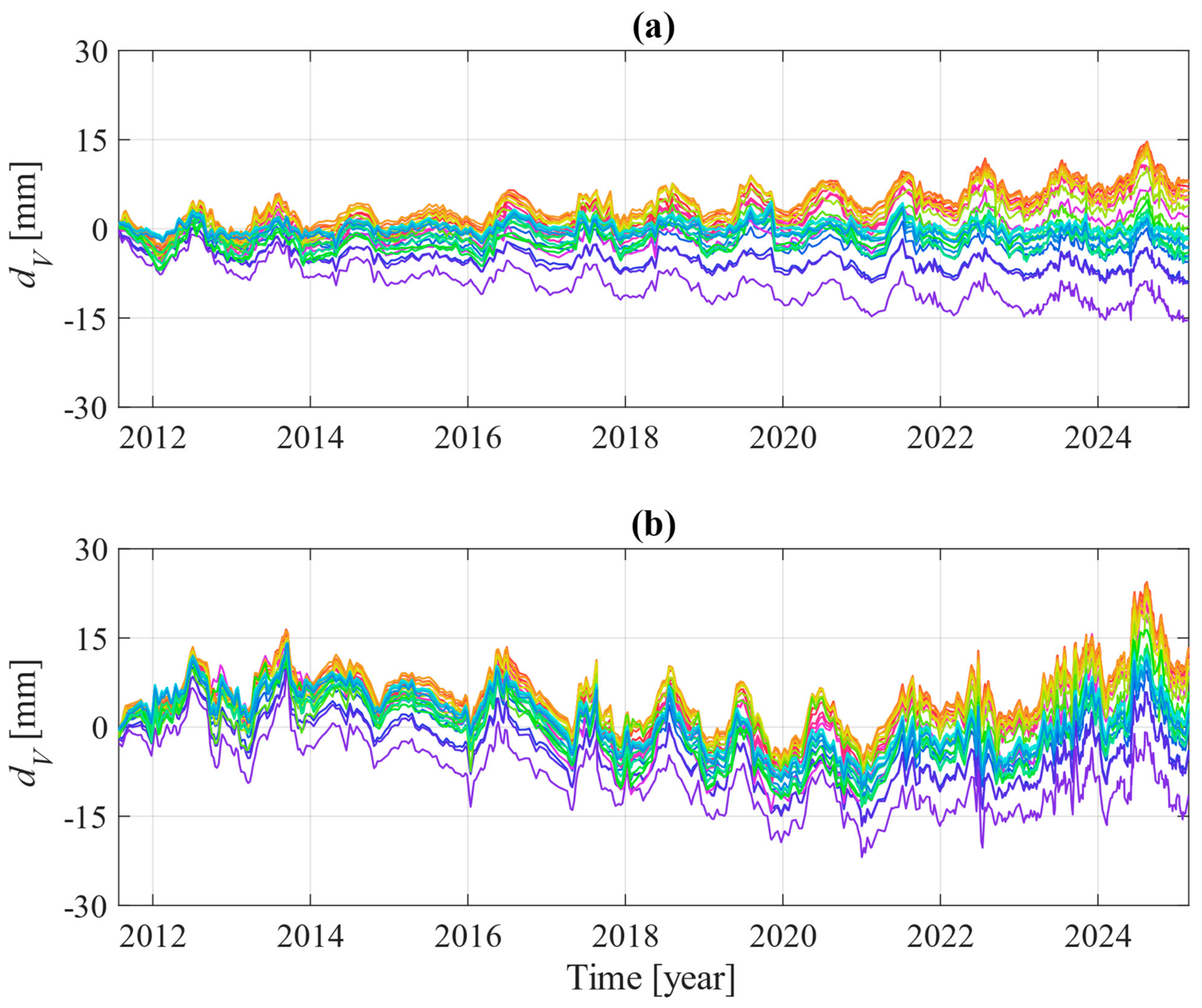
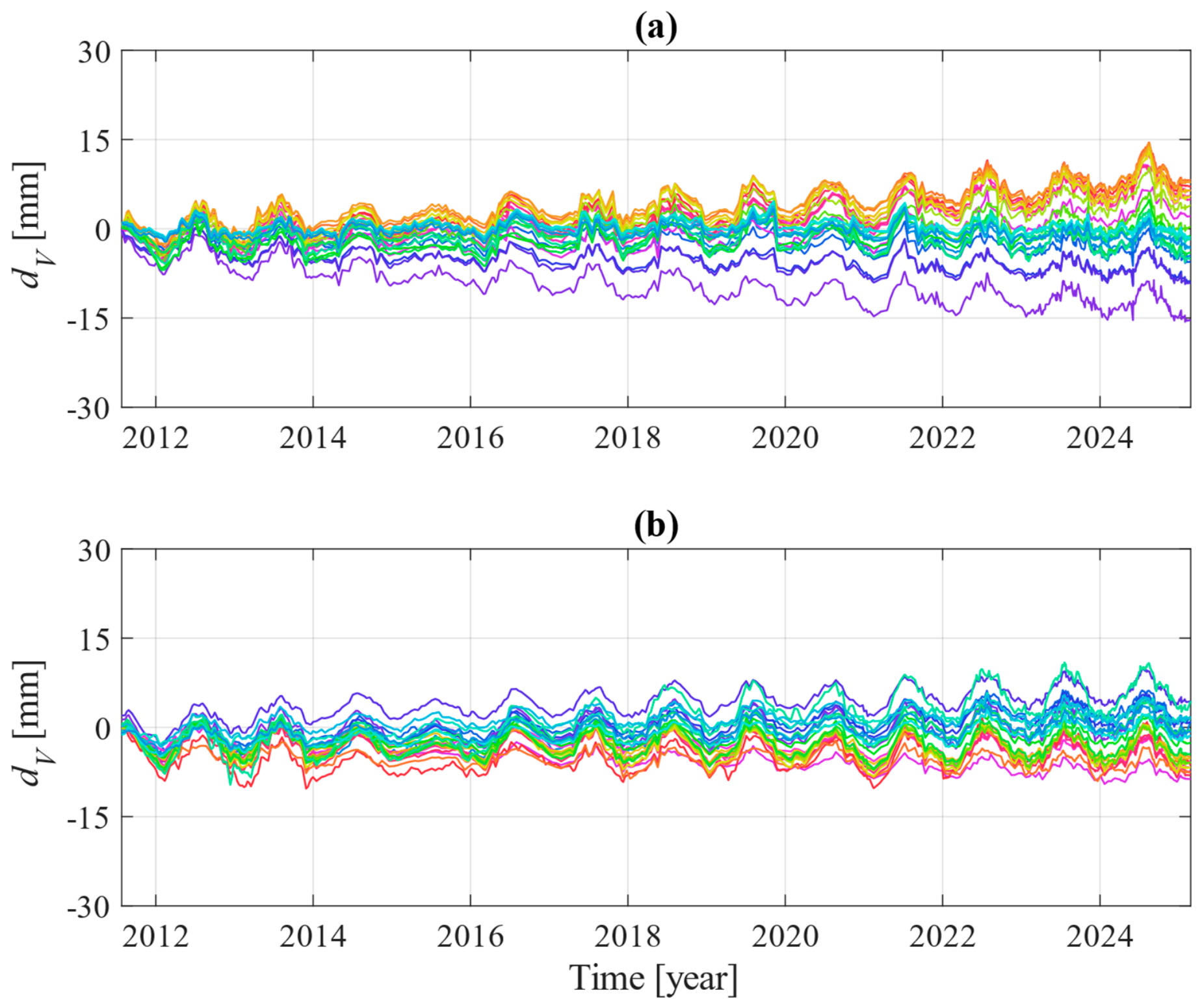
Figure 12 shows the reconstructed vertical displacement component d_V. After correction using the mean displacement of the reference PSs, a seasonal oscillation becomes clearly visible, consistent with the expected thermal response of the steel roof trusses. During warmer periods, thermal expansion of the radial trusses is expected to induce an upward displacement of the cantilevered roof elements, whereas the opposite behaviour is expected during colder periods. This seasonal pattern is less regular after correction using the polynomial fitting approach, which leaves higher short-term variability in the reconstructed time series.

Overall, the correction based on the mean displacement of the reference PSs leads to more regular time series than the polynomial-based correction. This suggests that, although the polynomial fit captures the main evolution of the background motion, it filters out shorter-term variations that are also present in the reference PSs and in the roof LOS measurements. As a result, these variations remain in the corrected time series and affect the reconstructed displacement components. The correction based on the mean displacement of the reference PSs is therefore adopted in the subsequent analysis.

Residual low-frequency trends are still visible in the time series after this correction. This indicates that the reference PSs extracted from the broader 1 km² area do not fully reproduce the local ground motion affecting all roof sectors. The reference PS selection is therefore refined in the following section by focusing on reference PSs located closer to the analysed roof areas.

4.3. Refinement of the Reference PSs Selection

To address the residual drift observed in the previous section, the compensation procedure was repeated using a more localised set of reference PSs. Specifically, instead of considering the PSs extracted from the 1 km² area surrounding the stadium, reference PSs were selected within a 20 m-wide band adjacent to the stadium perimeter. This band falls entirely on the open paved areas that surround the stadium and contains no buildings, so that all the PSs it includes lie on the ground and no further selection was required. For each roof area, a local reference cluster was defined using the neighbouring ground PSs, so that the estimated ground-related component could better represent the ground motion affecting that specific portion of the roof. Figure 13 shows the spatial distribution of the selected local clusters and the corresponding number of PSs available for the ascending and descending datasets. Area 13, for which no ascending PSs are available within the local band, was excluded from the following analysis.

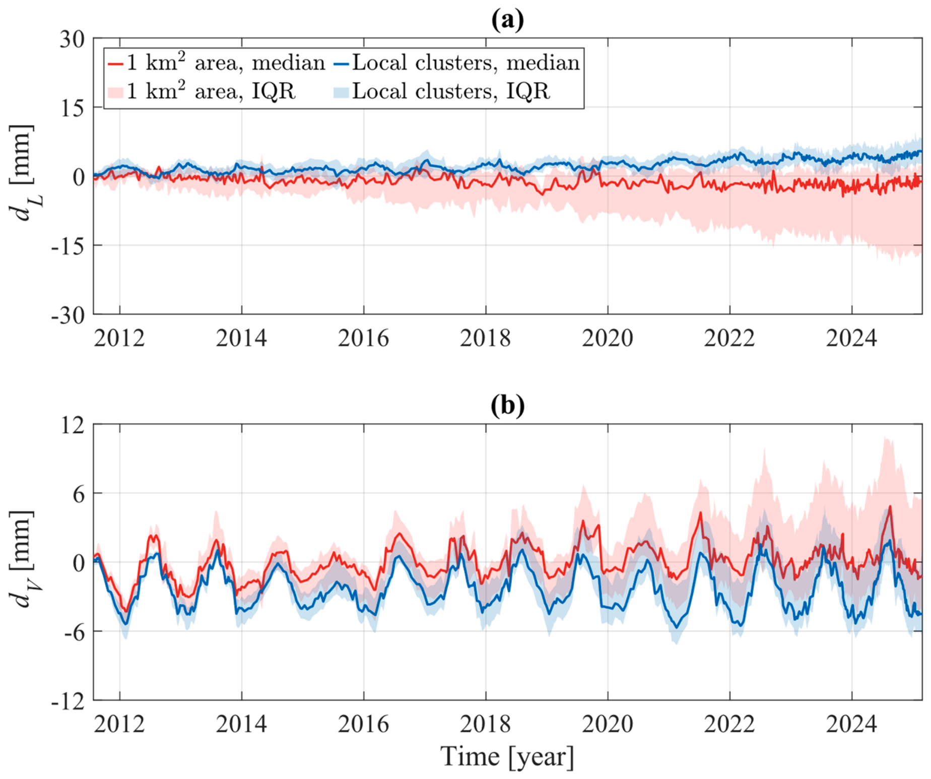
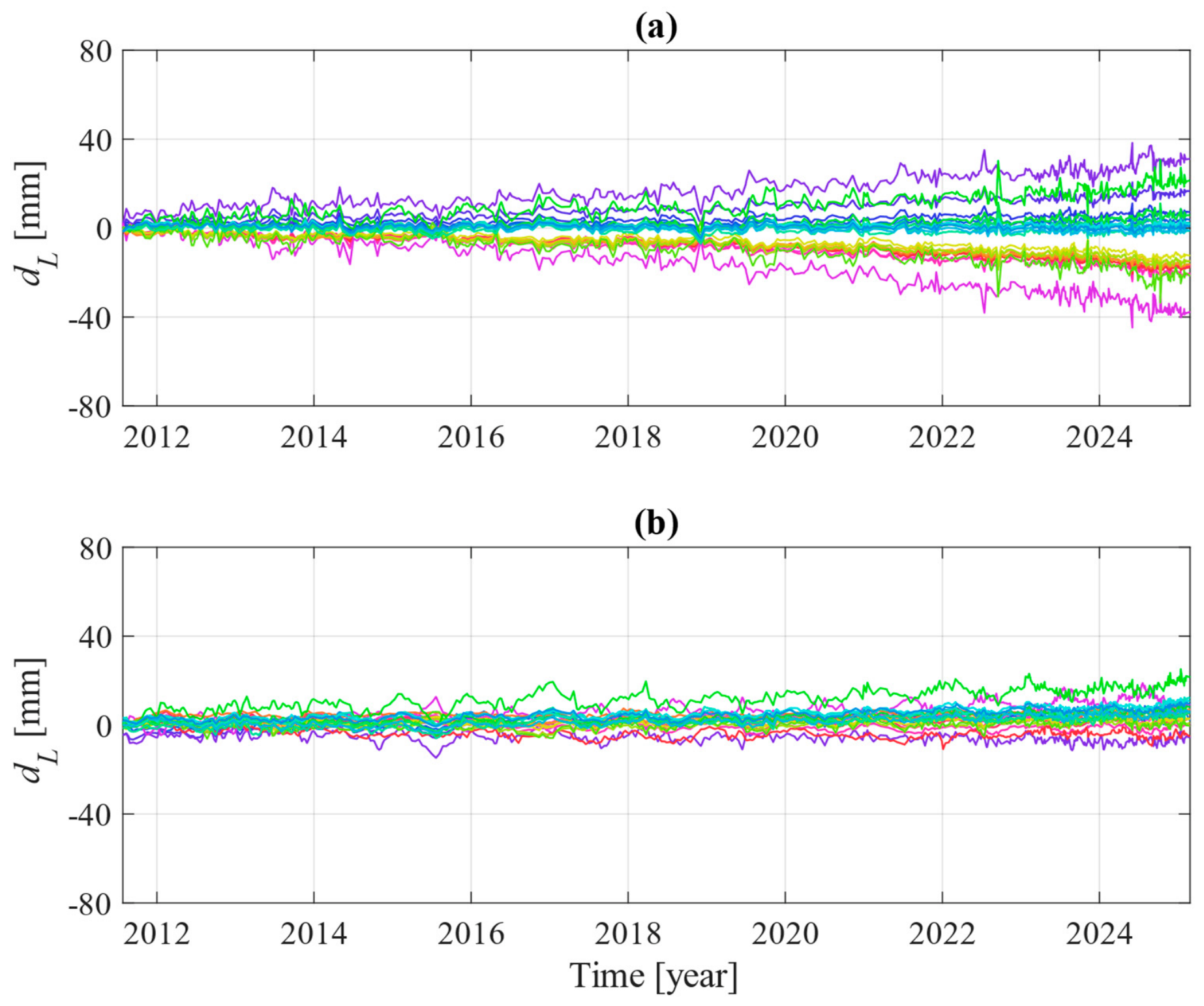
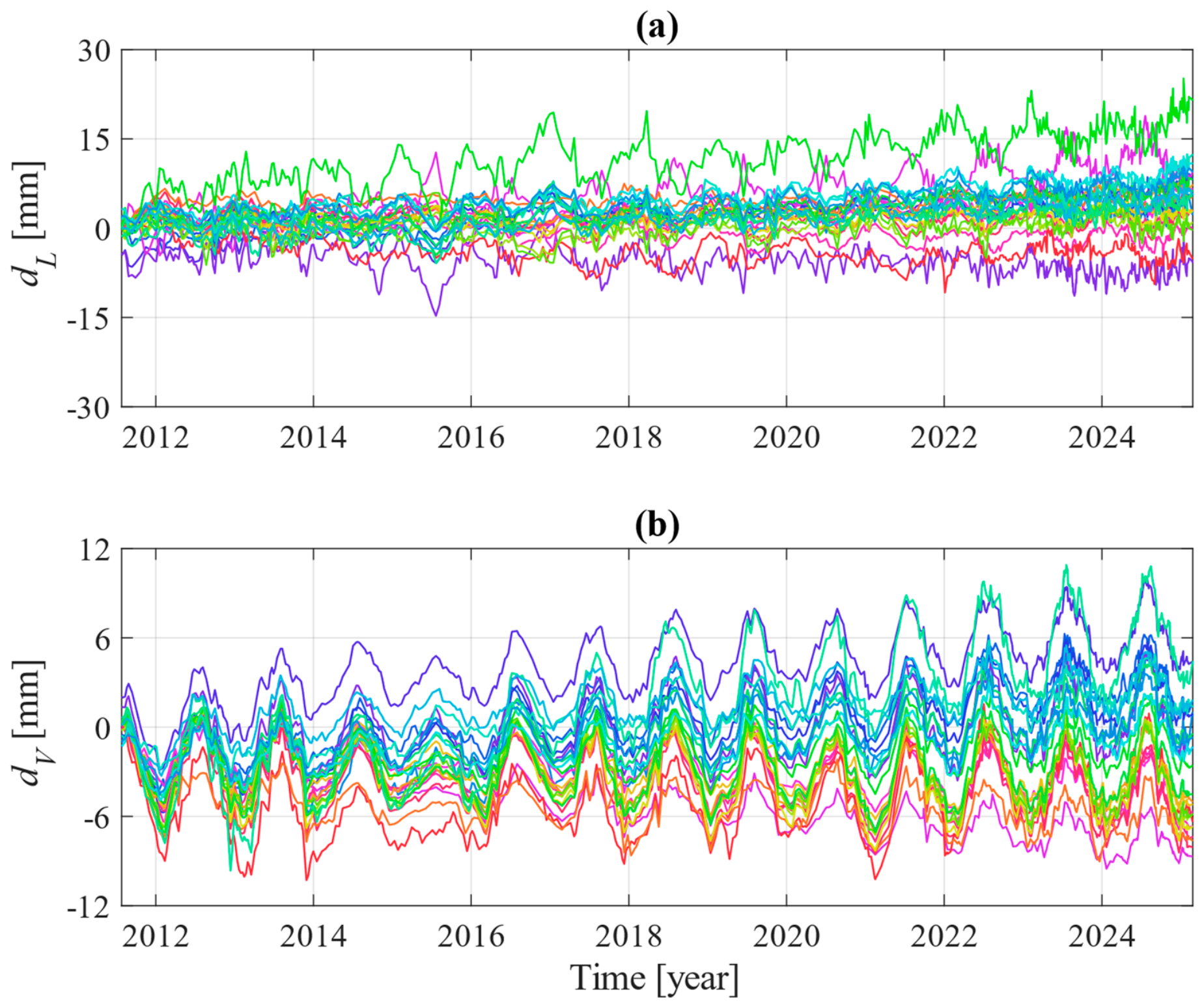
Figure 14 compares the reconstructed longitudinal displacements with those obtained in the previous section. Specifically, Figure 14a refers to the correction based on PSs within the 1 km² area, while Figure 14b refers to the correction based on the local reference clusters. In general, the residual displacement component is reduced when local reference clusters are used.

Figure 15 presents the same comparison for the vertical displacement component, d_V. Namely, Figure 15a shows the results obtained using the PSs within the 1 km² area, whereas Figure 15b shows results obtained using the local reference clusters. Also in this case, the local correction reduces part of the residual displacement component. The seasonal oscillation, which is consistent with the annual thermal response of the steel roof, is preserved. A moderate upward drift remains visible across the areas, especially in the vertical displacement time series.

In both Figure 14 and Figure 15, the two panels share the same scale, so that the reduction in the residual displacement obtained with the local clusters can be appreciated directly. Figure 16 reports the series obtained with the local clusters alone, on a scale adapted to their amplitude, allowing the behaviour of the individual areas to be followed. Figure 17 summarises the same comparison in statistical terms. At each acquisition date, the retained areas provide 25 values of the displacement component: the solid line is their median and the shaded band spans the Interquartile Range (IQR), that is, the interval between the first and third quartiles, so that it contains half of the areas at every date. Averaged over the whole observation period, the band narrows from 11.0 to 3.7 mm for d_L and from 5.3 to 3.7 mm for d_V when the reference PSs within the 1 km² area are replaced by the local reference clusters.

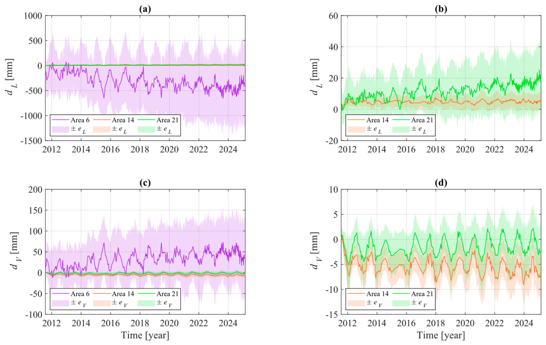
The error formulation of Section 2.3 is finally applied to the reconstructed components. Figure 18 reports the results obtained with the correction based on the local reference clusters for areas 6, 14, and 21, together with the error bounds calculated using Equation (23). The systematic contribution is evaluated assuming a transverse displacement of 1 mm. Areas 14 and 21 are, respectively, the best and worst-conditioned among the retained areas, while area 6 is one of the two excluded because of its ill-conditioned reconstruction, and is reinstated here as a term of comparison. Panels (a) and (c) include all three areas, whereas panels (b) and (d) focus on the two well-conditioned areas. The dispersion of the LOS measurements, evaluated at each acquisition time over the PSs contained in an area, ranges between 3.8 and 5.5 mm in both geometries, so that the differences between the error bounds originate almost entirely from the acquisition geometry. The same measurement dispersion produces errors one to two orders of magnitude larger for the ill-conditioned reconstruction. The bounds are not modified by the compensation, which subtracts from each area a single value at each acquisition date, common to all the PSs it contains, and therefore leaves their dispersion, and the error propagated from it, unchanged. The bounds shown in Figure 18 consequently apply equally to the uncorrected reconstruction of Section 4.1 and to the two correction strategies compared in Section 4.2.

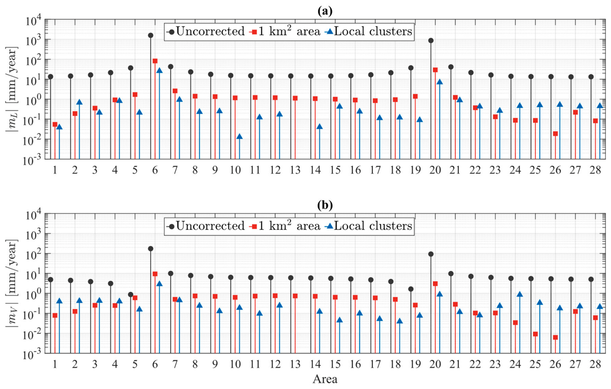
To quantify the effectiveness of the correction strategies, a linear trend was fitted to each reconstructed displacement time series. The absolute residual slope, |m_L,V|, was then used as an indicator of the residual long-term drift. Figure 19 compares this quantity for three cases: the uncorrected reconstruction, the correction based on the reference PSs within the 1 km² area, and the correction based on the local reference clusters. The slopes are shown on a logarithmic scale for both the longitudinal and vertical displacement components. Areas 6 and 20, excluded from the previous analysis because of their conditioning, are nevertheless reported for this comparison.

The correction based on the reference PSs within the 1 km² area reduces the mean absolute residual slope of the retained areas from 19.6 to 0.83 mm/year for the longitudinal component and from 5.5 to 0.39 mm/year for the vertical one, that is, by 96% and 93%, respectively. The correction based on the local reference clusters provides a further reduction to 0.34 and 0.23 mm/year, with residual slopes below 0.1 mm/year in several areas. However, this improvement is not uniform: in areas 23 to 28, and for the vertical component also in areas 1 to 4, the local correction leaves a larger residual slope than the correction based on the 1 km² area, although in all cases the residual remains below 0.9 mm/year.

This behaviour might be related to the spatial distribution of the reference PSs shown in Figure 13. Areas 24 to 28 contain between three and eight ascending PSs in their local band, and areas 1 and 2 contain one and three, respectively. The small number of ascending PSs may increase the uncertainty of the mean displacement used to estimate the ground-related component, potentially introducing additional variability rather than reducing the residual trend. However, PS availability alone does not explain all the results, as areas 3, 4, and 23 have denser ascending coverage but still exhibit a slight increase in the residual slope of the vertical component, of approximately 0.15 mm/year. Localised differential ground motion along this portion of the stadium cannot be excluded, and distinguishing the two effects would require reference clusters of comparable size across the perimeter.

5. Conclusions

This study investigated the use of satellite InSAR data for monitoring the displacement behaviour of the roof structure of the Diego Armando Maradona Stadium in Naples, Italy, a large steel structure located within the actively deforming Campi Flegrei caldera, where ground deformation dominates the displacement field observed over the surrounding urban area. High-resolution COSMO-SkyMed data were used and ascending and descending LOS measurements were combined to reconstruct displacement components in a local structural reference system.

The results demonstrate that regional ground deformation must be removed before the reconstructed displacements can be interpreted in terms of structural response. The polynomial model could not capture the short-term variability of the ground motion, which remained in the corrected time series. Conversely, the correction based on the mean displacement of the reference PSs produced smoother time series and revealed a clear seasonal pattern in the vertical displacement, consistent with the expected thermal response of the steel roof trusses.

Using reference PSs within the 1 km² area removed the dominant ground-motion trend but left residual drift in several roof areas. Selecting local ground PSs within a 20 m-wide band around the stadium and defining a separate reference cluster for each roof area further reduced the residual slopes. However, the effectiveness of this local correction decreased where only a few reference PSs were available, highlighting the trade-off between the spatial representativeness of the reference cluster and the number of observations used to estimate ground motion.

The reliability of the reconstruction also depended strongly on the orientation of the structural elements relative to the acquisition geometries. Error bounds remained within a few millimetres for the 26 retained areas but increased by one to two orders of magnitude for the two trusses oriented close to the satellite along-track direction. The displacement components reconstructed for these areas could therefore not be reliably interpreted.

The main limitation is the absence of independent roof-displacement measurements over the monitoring period. The corrected time series were consequently assessed only against the expected periodicity and phase of the seasonal structural response. Future research should integrate independent measurements covering at least one annual cycle and use temperature records and/or a finite element model to verify the thermal origin of the seasonal displacements. The ground-motion correction could also be refined by assessing different reference-area sizes and adopting regression models that explicitly quantify uncertainty when reference PSs are sparse or noisy.