Performance Evaluation of Vertical Bifacial Photovoltaic Modules for Building Applications in Land-Constrained Urban Environments

Abstract

In high-density cities, limited roof and ground areas constrain conventional photovoltaic (PV) deployment. Vertical bifacial photovoltaic (bPV) modules offer an alternative by making good use of building and infrastructure surfaces while harvesting irradiance on both sides. This study develops an integrated module-level framework for evaluating tilted and vertical bPV modules. It couples two-sided anisotropic irradiance calculations with five-parameter electrical and steady-state thermal models. Unlike irradiance-only or configuration-specific assessments, the framework consistently compares bPV and monofacial PV (mPV) modules across tilt and azimuth configurations while jointly quantifying power output, module temperature, bifacial gain, and angular losses. Predicted power output agreed well with outdoor measurements across four representative mounting configurations, and annual predictions were comparable to PVsyst and SAM results. Applied to Hong Kong, the framework identified optimum tilt angles of approximately 20° for bPV and 18° for mPV modules. A vertical west-facing bPV module achieved 96.3% of the annual energy yield of optimally tilted mPV, with a bifacial gain of 67.2% and an angular-loss-related power loss of 4.8%. These results show that vertical bPV can approach optimally tilted mPV performance while utilizing otherwise unused building surfaces, supporting preliminary design decisions in land-constrained cities.

1. Introduction

In compact cities, conventional roof- and ground-mounted PV systems are constrained by limited roof area, high-rise urban morphology, competing building services, mutual shading, and land use pressure [1]. This challenge is particularly relevant to Hong Kong, where dense development restricts large horizontal PV installations [2]. Installing PV modules vertically or near vertically on building and infrastructure surfaces therefore offers an important opportunity to expand urban PV deployment.

Bifacial photovoltaic (bPV) modules are well suited to these mounting configurations because they collect irradiance from both the front and rear sides [3,4,5]. By harvesting diffuse and ground-reflected irradiance on the rear surface, they can improve energy yield per module area. Accordingly, vertical bPV modules can be incorporated into facades, balustrades, noise barriers, fences, and other building or infrastructure elements, with the potential to deliver favourable energy performance [6,7,8,9]. Their performance, however, depends jointly on tilt angle, azimuth angle, surrounding reflectance, module temperature, and angular optical losses. These coupled effects must be considered together to provide reliable design guidance.

Existing bPV research has addressed irradiance modelling, system simulation, and specific applications. Guo et al. [10] analyzed vertical east- and west-facing modules using beam and diffuse irradiance calculations, although anisotropic ground-reflected irradiance was not fully represented. Sun et al. [11] combined the Perez model with an anisotropic treatment of ground-reflected irradiance that considered module self-shading. Rodríguez-Gallegos et al. [12,13] applied Marion’s method and assessed the techno-economic performance of bifacial and tracking systems. Gu et al. [14] developed a coupled optical–electrical–thermal model for short- and long-term evaluation. Vertical bPV has also been examined in a rooftop balustrade application [8]. However, differences in configurations, model boundaries, and performance indicators hinder consistent comparison among tilted and vertical bPV and mPV systems. A consistent module-level framework linking two-sided irradiance, temperature, and electrical output is therefore still needed for building applications.

Accurate treatment of both module surfaces is particularly important because irradiance determines electrical output and module temperature. Module shadows can create non-uniform ground irradiance [9,15], while the shaded region can switch sides for vertical east- and west-facing modules; approaches emphasizing rear-side anisotropy may therefore be insufficient [16,17]. The concise anisotropic model in [5] experimentally validated two-sided irradiance estimates for horizontal, tilted, and vertical bPV modules. Its scope, however, was irradiance prediction and did not extend to module temperature, electrical output, or annual energy performance indicators.

Thermal and electrical responses must subsequently be coupled to irradiance. Single-point power models [7,11] and the nominal operating cell temperature model [18] are computationally efficient but cannot fully represent module behaviour under variable weather. Equivalent circuit and heat transfer models provide greater physical detail [7,9] but increase the computational cost of annual simulation. Building-related assessment therefore requires an efficient and physically interpretable treatment of power–temperature coupling.

Existing studies therefore provide valuable component-level or application-specific analyses, but systematic evaluation of tilted and vertical bPV and monofacial PV (mPV) configurations remains limited. In particular, few studies combine outdoor power validation, annual benchmarking against established software, and joint assessment of energy yield, bifacial gain, module temperature, and angular losses within one framework. Such an assessment is needed to establish the energy performance potential of vertical bPV where horizontal installation area is restricted.

Accordingly, this study develops an integrated module-level framework for evaluating bPV modules in land-constrained building applications. It couples a two-sided anisotropic irradiance calculation with a simplified heat transfer model and a five-parameter electrical model, using Newton’s method to solve module temperature and power output simultaneously. Power output predictions are evaluated against outdoor measurements, and annual predictions are benchmarked against PVsyst and SAM. The framework is then applied in Hong Kong to compare tilted and vertical bPV and mPV configurations in terms of annual energy yield, bifacial gain, module temperature, and angular-loss-related power loss. By linking two-sided irradiance to thermal and electrical behaviour across consistent configurations, the study provides an integrated comparative basis for vertical bPV applications on facades, balustrades, noise barriers, and other urban building surfaces.

2. Theoretical Modelling

2.1. Irradiance Model

The solar geometry was first obtained from the NREL solar position algorithm, which provides the solar zenith angle and solar azimuth angle for each simulation time step [19].

For either module face, the incident irradiance was separated into direct-beam, sky-diffuse, and ground-reflected terms [5,7,9]:

$$G=G_{\mathrm{b}}+G_{\mathrm{d}}+G_{\mathrm{r}}$$

(1)

where $G_{\mathrm{b}}$, $G_{\mathrm{d}}$ and $G_{\mathrm{r}}$ denote the beam, diffuse, and ground-reflected irradiance components incident on the considered module surface.

The beam component was derived from the direct normal irradiance and the incidence angle between the sun beam and the module surface [7,9]:

$$G_{\mathrm{b}}=\mathrm{D}\mathrm{N}\mathrm{I}\mathrm{c}\mathrm{o}\mathrm{s}\theta =(\mathrm{G}\mathrm{H}\mathrm{I}-\mathrm{D}\mathrm{H}\mathrm{I})\mathrm{c}\mathrm{o}\mathrm{s}\theta /\mathrm{c}\mathrm{o}\mathrm{s}z$$

(2)

where direct normal irradiance, global horizontal irradiance, and diffuse horizontal irradiance are denoted by DNI, GHI, and DHI, respectively. $z$ is the solar zenith, $\theta$ is the incidence angle and the front-side incidence angle was calculated from the solar position and module orientation [12]:

$$\mathrm{c}\mathrm{o}\mathrm{s}\theta =\mathrm{c}\mathrm{o}\mathrm{s}z·\mathrm{c}\mathrm{o}\mathrm{s}\beta +\mathrm{s}\mathrm{i}\mathrm{n}z·\mathrm{s}\mathrm{i}\mathrm{n}\beta ·\mathrm{c}\mathrm{o}\mathrm{s}({\gamma }_{\mathrm{s}}-{\gamma }_{\mathrm{m}})$$

(3)

where $\beta$ is the module tilt angle, ${\gamma }_{\mathrm{s}}$ and ${\gamma }_{\mathrm{m}}$ are the azimuths of the sun and module. For rear-side calculation, the corresponding rear orientation was used by transforming the front-side tilt and azimuth.

The sky-diffuse component on an inclined surface was evaluated using the Perez anisotropic sky model [20,21,22]:

$$G_{\mathrm{d}}=\mathrm{D}\mathrm{H}\mathrm{I}\left(1-F_1\right){\displaystyle \frac{1+\mathrm{c}\mathrm{o}\mathrm{s}\beta }{2}}+F_1{\displaystyle \frac{a}{b}}+F_2\mathrm{s}\mathrm{i}\mathrm{n}\beta$$

(4)

where the empirical coefficients ($F_1$, $F_2$, $a$, and $b$) in the Perez model were taken from the original formulation [22]. The same orientation conversion was used when the rear-side diffuse irradiance was calculated.

Ground reflection was treated separately because module shading changes the irradiance distribution over the ground plane. For south-facing tilted modules, this effect is often most evident behind the module. For vertical or east-/west-facing modules, however, the shaded part of the ground may alternate between the two sides. The reflected component was therefore calculated with a two-dimensional view factor method that distinguishes shaded and unshaded ground areas [5,7,9,16]:

$$G_{\mathrm{r}}=\rho F_{\mathrm{m}\to \mathrm{u}\mathrm{s}\mathrm{g}\mathrm{r}\mathrm{d}}\mathrm{G}\mathrm{H}\mathrm{I}+\rho F_{\mathrm{m}\to \mathrm{s}\mathrm{g}\mathrm{r}\mathrm{d}}\mathrm{D}\mathrm{H}\mathrm{I}$$

(5)

where $\rho$ is the ground albedo, and $F_{\mathrm{m}\to \mathrm{u}\mathrm{s}\mathrm{g}\mathrm{r}\mathrm{d}}$ and $F_{\mathrm{m}\to \mathrm{s}\mathrm{g}\mathrm{r}\mathrm{d}}$ are the view factors from the module surface to the unshaded and shaded ground, respectively. In this formulation, the ground on one side of the module is divided into shaded and unshaded regions only when direct-beam irradiance reaches the opposite module side.

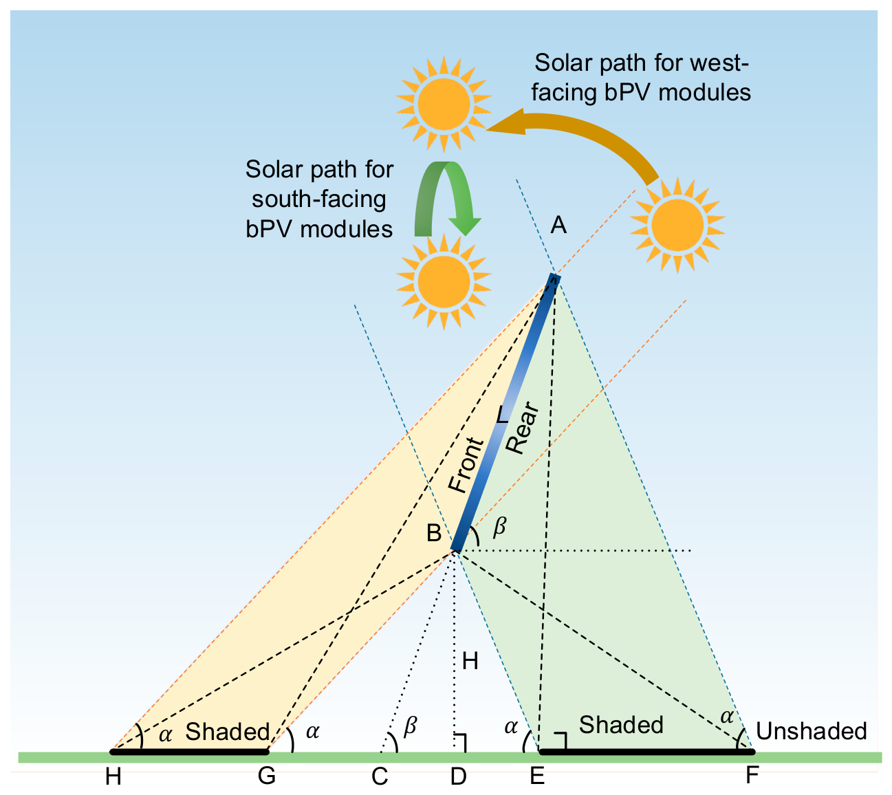
The remaining task is the geometric evaluation of view factors between each module face and the corresponding ground regions. Figure 1 shows the adopted geometry. A conventional south-facing tilted module mainly casts its shadow behind the module, whereas a vertical east- or west-facing module can experience a front-to-rear switch of the shaded region as the sun moves.

For the shaded-ground exchange, the cross-string rule was used to convert the geometric boundary lengths into the required view factors [23]:

$$F_{\mathrm{R}\to \mathrm{s}\mathrm{g}\mathrm{r}\mathrm{d}}={\displaystyle \frac{\mathrm{A}\mathrm{E}+\mathrm{B}\mathrm{F}-\mathrm{B}\mathrm{E}-\mathrm{A}\mathrm{F}}{2L}}$$

(6)

where the line segments AE, BF, BE, and AF define the geometric paths used for calculating the rear surface view factor to the shaded ground.

The corresponding front-side shaded-ground term is obtained from the analogous set of geometric lengths:

$$F_{\mathrm{F}\to \mathrm{s}\mathrm{g}\mathrm{r}\mathrm{d}}={\displaystyle \frac{\mathrm{A}\mathrm{G}+\mathrm{B}\mathrm{H}-\mathrm{B}\mathrm{G}-\mathrm{A}\mathrm{H}}{2L}}$$

(7)

where the segments AG, BH, BG, and AH are the corresponding geometric lengths for the front-side calculation.

The sky-view terms were obtained from the module tilt geometry as follows [16]:

$$\begin{gathered} F_{\mathrm{R}\to \mathrm{s}\mathrm{k}\mathrm{y}}={\displaystyle \frac{1-\mathrm{c}\mathrm{o}\mathrm{s}\beta }{2}} \\ {F}_{\mathrm{F}\to \mathrm{s}\mathrm{k}\mathrm{y}}={\displaystyle \frac{1+\mathrm{c}\mathrm{o}\mathrm{s}\beta }{2}} \end{gathered}$$

(8)

Because the view factors from a module face to the sky, shaded ground, and unshaded ground sum to unity, the unshaded ground view factor can be obtained by difference [16]:

$$F_{\mathrm{F}/\mathrm{R}\to \mathrm{s}\mathrm{g}\mathrm{r}\mathrm{d}}+F_{\mathrm{F}/\mathrm{R}\to \mathrm{u}\mathrm{s}\mathrm{g}\mathrm{r}\mathrm{d}}+F_{\mathrm{F}/\mathrm{R}\to \mathrm{s}\mathrm{k}\mathrm{y}}=1$$

(9)

In each simulation scenario, the ground was assumed to be flat and Lambertian, with a spatially uniform and time-invariant broadband albedo. The albedo range of 0.1–0.8 was used to represent the different reflectance levels of common urban surfaces, ranging from dark asphalt to concrete or paving blocks and high-reflectance coatings. The view factor geometry further assumes unobstructed surroundings and accounts only for the shadow cast by the PV module itself; shading and view obstruction caused by adjacent buildings, parapets, vegetation, or other urban objects were not explicitly represented. For spatially heterogeneous surfaces, the model can be extended by dividing the ground into material-specific patches and summing their reflected irradiance contributions according to the corresponding albedo, incident irradiance, and view factor.

Incidence angle reflection was represented with the analytical angular loss model of Martin and Ruiz [24,25]. The correction factors for the beam, diffuse, and ground-reflected components were determined as follows:

$$\begin{gathered} f_{\mathrm{b}}={\displaystyle \frac{\exp \left(-\cos \left(\frac{\theta }{a_{\mathrm{r}}}\right)\right)-\exp \left(-\frac{1}{a_{\mathrm{r}}}\right)}{1-\exp \left(-\frac{1}{a_{\mathrm{r}}}\right)}} \\ {f}_{\mathrm{d}}=\exp \left[-{\displaystyle \frac{1}{a_{\mathrm{r}}}}\left(c_1\left(\mathrm{s}\mathrm{i}\mathrm{n}\beta +{\displaystyle \frac{\pi -\beta -\mathrm{s}\mathrm{i}\mathrm{n}\beta }{1+\mathrm{c}\mathrm{o}\mathrm{s}\beta }}\right)+c_2{\left(\mathrm{s}\mathrm{i}\mathrm{n}\beta +{\displaystyle \frac{\pi -\beta -\mathrm{s}\mathrm{i}\mathrm{n}\beta }{1+\mathrm{c}\mathrm{o}\mathrm{s}\beta }}\right)}^2\right)\right] \\ {f}_{\mathrm{r}}=\exp \left[-{\displaystyle \frac{1}{a_{\mathrm{r}}}}\left(c_1\left(\mathrm{s}\mathrm{i}\mathrm{n}\beta +{\displaystyle \frac{\beta -\mathrm{s}\mathrm{i}\mathrm{n}\beta }{1-\mathrm{c}\mathrm{o}\mathrm{s}\beta }}\right)+c_2{\left(\mathrm{s}\mathrm{i}\mathrm{n}\beta +{\displaystyle \frac{\beta -\mathrm{s}\mathrm{i}\mathrm{n}\beta }{1-\mathrm{c}\mathrm{o}\mathrm{s}\beta }}\right)}^2\right)\right] \end{gathered}$$

(10)

where angular loss factors ($f_{\mathrm{b}}$, $f_{\mathrm{d}}$ and $f_{\mathrm{r}}$) correspond to the beam, diffuse, and ground-reflected components, respectively. The coefficient $a_{\mathrm{r}}$ and the other empirical parameters follow the Martin and Ruiz model [24]. Rear-side angular losses were calculated using the rear-side orientation defined above.

The effective irradiance on each module face was finally obtained by applying the corresponding angular loss factor to each irradiance component:

$$G=G_{\mathrm{b}}(1-f_{\mathrm{b}})+G_{\mathrm{d}}(1-f_{\mathrm{d}})+G_{\mathrm{r}}(1-f_{\mathrm{r}})$$

(11)

This formulation provides a compact two-sided anisotropic irradiance calculation for bPV modules under horizontal, tilted, and vertical configurations.

2.2. Electrical Model

The electrical response was represented using the five-parameter model reported by Ma et al. [26], which provides a practical balance between physical detail and computational efficiency. The current–voltage relationship is written as [26]:

$$I=I_{\mathrm{p}\mathrm{h}}-I_0\left(\exp \left({\displaystyle \frac{V+R_{\mathrm{s}}I}{N_{\mathrm{s}}{V}_{\mathrm{t}}}}\right)-1\right)-{\displaystyle \frac{V+R_{\mathrm{s}}I}{R_{\mathrm{p}}}}$$

(12)

where $I_{\mathrm{p}\mathrm{h}}$ is the light-generated (photo) current, $I_0$ is the reserve saturation current of the diode, $R_{\mathrm{s}}$ is the module series resistance, $N_{\mathrm{s}}$ is the cell number in series in one module, $V_{\mathrm{t}}$ is the diode thermal voltage, and $R_{\mathrm{p}}$ is the module parallel resistance.

Under standard test conditions (STCs), the same relationship can be expressed in the reference form [26]:

$$I=I_{\mathrm{p}\mathrm{h},\mathrm{r}\mathrm{e}\mathrm{f}}-I_{0,\mathrm{r}\mathrm{e}\mathrm{f}}\left(\exp \left({\displaystyle \frac{V+R_{\mathrm{s},\mathrm{r}\mathrm{e}\mathrm{f}}I}{N_{\mathrm{s}}{V}_{\mathrm{t},\mathrm{r}\mathrm{e}\mathrm{f}}}}\right)-1\right)-{\displaystyle \frac{V+R_{\mathrm{s},\mathrm{r}\mathrm{e}\mathrm{f}}I}{R_{\mathrm{p},\mathrm{r}\mathrm{e}\mathrm{f}}}}$$

(13)

where the subscript ‘ref’ indicates that the corresponding quantities are evaluated at STC.

The five reference parameters in the STC equation were extracted from the manufacturer’s datasheet following the procedure described in [26]. The datasheet values of short circuit current, open circuit voltage, maximum power point current, maximum power point voltage, and the number of series-connected cells were used as inputs. The single-diode equations were constrained at the short circuit, open circuit, and maximum power points, together with the condition (dP/dV = 0) at the maximum power point. The resulting nonlinear algebraic equations were solved simultaneously to obtain $I_{\mathrm{p}\mathrm{h},\mathrm{r}\mathrm{e}\mathrm{f}}$, $I_{0,\mathrm{r}\mathrm{e}\mathrm{f}}$, $R_{\mathrm{s},\mathrm{r}\mathrm{e}\mathrm{f}}$, $R_{\mathrm{p},\mathrm{r}\mathrm{e}\mathrm{f}}$, and $V_{\mathrm{t},\mathrm{r}\mathrm{e}\mathrm{f}}$. These reference parameters were then adjusted to the actual irradiance and module temperature conditions using the relationships given in [14]:

$$\begin{gathered} I_{\mathrm{p}\mathrm{h}}={\displaystyle \frac{G_{\mathrm{F}}+{\mathrm{B}\mathrm{F}·G}_{\mathrm{R}}}{G_{\mathrm{r}\mathrm{e}\mathrm{f}}}}{I}_{\mathrm{p}\mathrm{h},\mathrm{r}\mathrm{e}\mathrm{f}}(1+\lambda \left(T-T_{\mathrm{r}\mathrm{e}\mathrm{f}}\right)) \\ {I}_0=I_{0,\mathrm{r}\mathrm{e}\mathrm{f}}{\left({\displaystyle \frac{T}{T_{\mathrm{r}\mathrm{e}\mathrm{f}}}}\right)}^3\mathrm{e}\mathrm{x}\mathrm{p}\left({\displaystyle \frac{q_{\mathrm{e}}{E}_{\mathrm{g}}}{K}}\left({\displaystyle \frac{1}{T}}-{\displaystyle \frac{1}{T_{\mathrm{r}\mathrm{e}\mathrm{f}}}}\right)\right) \\ {R}_{\mathrm{s}}=R_{\mathrm{s},\mathrm{r}\mathrm{e}\mathrm{f}} \\ {V}_{\mathrm{t}}={\displaystyle \frac{T}{T_{\mathrm{r}\mathrm{e}\mathrm{f}}}}{V}_{\mathrm{t},\mathrm{r}\mathrm{e}\mathrm{f}} \\ {R}_{\mathrm{p}}={\displaystyle \frac{G_{\mathrm{r}\mathrm{e}\mathrm{f}}}{G_{\mathrm{F}}+{\mathrm{B}\mathrm{F}·G}_{\mathrm{R}}}}{R}_{\mathrm{p},\mathrm{r}\mathrm{e}\mathrm{f}} \end{gathered}$$

(14)

where $G_{\mathrm{F}}$ $\mathrm{a}\mathrm{n}\mathrm{d}$ $G_{\mathrm{R}}$ are the irradiance received by the front and rear surfaces, $\mathrm{B}\mathrm{F}$ is the module bifaciality, $\lambda$ is the temperature coefficient of short circuit current, $T$ is the cell temperature, $q_{\mathrm{e}}$ is the charge of electron (1.602 × 10⁻¹⁹ C), $E_{\mathrm{g}}$ is the band gap (1.7936 × 10⁻¹⁹ J), $K$ is the Boltzmann’s constant (1.381 × 10⁻²³ J/K), and $G_{\mathrm{r}\mathrm{e}\mathrm{f}}$ and $T_{\mathrm{r}\mathrm{e}\mathrm{f}}$ are the reference irradiance and cell temperature ($G_{\mathrm{r}\mathrm{e}\mathrm{f}}=1000 \mathrm{W}/{\mathrm{m}}^2$ and $T_{\mathrm{r}\mathrm{e}\mathrm{f}}=25 °\mathrm{C}$), respectively.

The maximum power point was obtained from the calculated I-V curve. When other loss mechanisms were not included, the module output power was calculated as:

$$P_{\mathrm{m}\mathrm{a}\mathrm{x}}=I_{\mathrm{m}\mathrm{p}\mathrm{p}}{V}_{\mathrm{m}\mathrm{p}\mathrm{p}}$$

(15)

where the subscript ‘mpp’ denotes the maximum power point.

2.3. Thermal Model

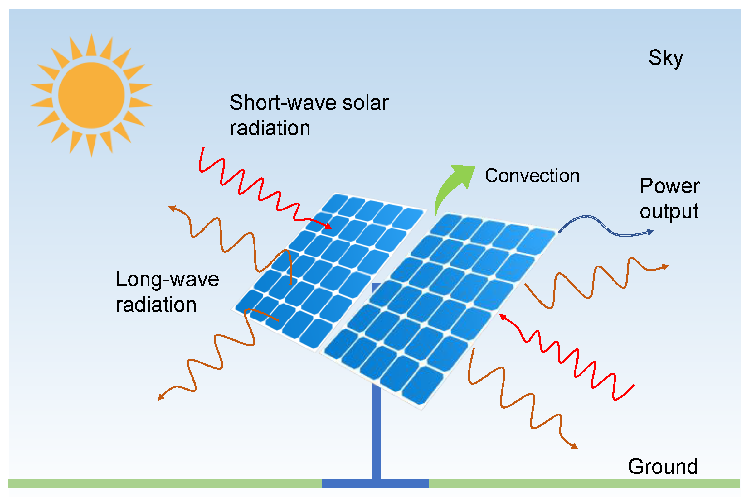
A steady-state heat transfer model was used instead of a simple empirical temperature model. The steady-state assumption was adopted because the principal objective of the model is hourly and annual energy performance assessment using typical meteorological year data. Each simulation time step was therefore treated as a quasi-steady operating condition, and the thermal capacitance term was neglected. This treatment provides a computationally efficient estimate of module temperature for long-term simulations. However, it does not reproduce the thermal lag of the module during rapid irradiance variations, such as passing clouds, and should not be interpreted as a transient temperature model. Figure 2 illustrates the exchange of heat between a PV module and its surroundings through long-wave radiation and convection, while the absorbed solar energy and electrical output enter the module energy balance.

Under steady-state conditions, the module energy balance can be written as:

$$(q_{\mathrm{s}\mathrm{w}}+q_{\mathrm{l}\mathrm{w}}+q_{\mathrm{c}\mathrm{o}\mathrm{n}\mathrm{v}})A=P_{\mathrm{o}\mathrm{u}\mathrm{t}}$$

(16)

where $q_{\mathrm{s}\mathrm{w}}$ is the short-wave solar radiation absorbed by the module, $q_{\mathrm{l}\mathrm{w}}$ is the long-wave radiation, $q_{\mathrm{c}\mathrm{o}\mathrm{n}\mathrm{v}}$ is the convective heat exchange, $A$ is the module area and $P_{\mathrm{o}\mathrm{u}\mathrm{t}}$ is the power output.

The absorbed short-wave radiation was calculated from the irradiance incident on the module and the corresponding absorption coefficient [27]:

$$q_{\mathrm{s}\mathrm{w}}=\phi G={\phi }_{\mathrm{F}}{G}_{\mathrm{F}}+{\phi }_{\mathrm{R}}{G}_{\mathrm{R}}$$

(17)

where $\phi$ is the absorption coefficient of the module. For bifacial modules with a double-glass structure, it is considered that ${\phi }_{\mathrm{F}}={\phi }_{\mathrm{R}}=1$ since the reflection loss was considered in the irradiance model. For monofacial modules with a glass cover and a white back sheet, it is considered that ${\phi }_{\mathrm{F}}=1$ while ${\phi }_{\mathrm{R}}=0.7$ [28].

The long-wave radiative exchange between the module, the sky, and the ground was calculated by [29]:

$$\begin{gathered} q_{\mathrm{l}\mathrm{w}\to \mathrm{g}\mathrm{r}\mathrm{d}}=\sigma F_{\mathrm{F}\to \mathrm{g}\mathrm{r}\mathrm{d}}\left({{\epsilon }_{\mathrm{g}\mathrm{r}\mathrm{d}}{T}_{\mathrm{g}\mathrm{r}\mathrm{d}}^4-{\epsilon }_{\mathrm{F}}T}_{\mathrm{m}}^4\right)+\sigma F_{\mathrm{R}\to \mathrm{g}\mathrm{r}\mathrm{d}}\left({\epsilon }_{\mathrm{g}\mathrm{r}\mathrm{d}}{T_{\mathrm{g}\mathrm{r}\mathrm{d}}^4-{\epsilon }_{\mathrm{R}}T}_{\mathrm{m}}^4\right) \\ {q}_{\mathrm{l}\mathrm{w}\to \mathrm{s}\mathrm{k}\mathrm{y}}=\sigma F_{\mathrm{F}\to \mathrm{s}\mathrm{k}\mathrm{y}}\left({\epsilon }_{\mathrm{s}\mathrm{k}\mathrm{y}}{T_{\mathrm{s}\mathrm{k}\mathrm{y}}^4-{\epsilon }_{\mathrm{F}}T}_{\mathrm{m}}^4\right)+\sigma F_{\mathrm{R}\to \mathrm{s}\mathrm{k}\mathrm{y}}\left({{\epsilon }_{\mathrm{s}\mathrm{k}\mathrm{y}}{T}_{\mathrm{s}\mathrm{k}\mathrm{y}}^4-{\epsilon }_{\mathrm{R}}T}_{\mathrm{m}}^4\right) \end{gathered}$$

(18)

where $\sigma$ is the Boltzmann constant (5.67 × 10^-8 W/m²/K⁴), $\epsilon$ is the emissivity, and the subscript ‘grd’ represents the ground. According to the available data in the literature, the parameters settings in this equation are as follows: $T_{\mathrm{g}\mathrm{r}\mathrm{d}}=T_{\mathrm{a}}$ and ${\epsilon }_{\mathrm{g}\mathrm{r}\mathrm{d}}=0.95$ [27], $T_{\mathrm{s}\mathrm{k}\mathrm{y}}=T_{\mathrm{a}}-11$ and ${\epsilon }_{\mathrm{s}\mathrm{k}\mathrm{y}}=0.8$ (the relation was adopted as a simplified approximation of the effective sky temperature for the hourly and annual simulations in Hong Kong. Variations associated with cloud cover, atmospheric humidity, and season were not explicitly resolved and may introduce some uncertainty into the predicted absolute module temperature) [30], ${\epsilon }_{\mathrm{F}}=0.91$ for the front glass, ${\epsilon }_{\mathrm{R}}=0.91$ for the back glass, and ${\epsilon }_{\mathrm{R}}=0.85$ for the white back sheet (Teldar) [31].

Convective heat transfer between the module and ambient air was expressed as:

$$q_{\mathrm{c}\mathrm{o}\mathrm{n}\mathrm{v}}=h_{\mathrm{c}\mathrm{o}\mathrm{n}\mathrm{v}}(T_{\mathrm{a}}-T_{\mathrm{m}})$$

(19)

where $h_{\mathrm{c}\mathrm{o}\mathrm{n}\mathrm{v}}$ is the overall convection heat transfer coefficient.

The overall convection term includes both natural and forced components. Natural convection was evaluated using the following empirical relation [27,32]:

$$h_{\mathrm{c}\mathrm{o}\mathrm{n}\mathrm{v},\mathrm{f}\mathrm{r}\mathrm{e}\mathrm{e}}=1.31{(T_{\mathrm{a}}-T_{\mathrm{m}})}^{1/3}$$

(20)

Forced convection was represented by the wind-speed-dependent correlation [33]:

$$h_{\mathrm{c}\mathrm{o}\mathrm{n}\mathrm{v},\mathrm{f}\mathrm{o}\mathrm{r}\mathrm{c}\mathrm{e}\mathrm{d}}=2.8+3u_{\mathrm{w}}$$

(21)

where $u_{\mathrm{w}}$ is the wind speed.

The natural and forced convection coefficients were combined to obtain the overall convective heat transfer coefficient [31,33]:

$$h_{\mathrm{c}\mathrm{o}\mathrm{n}\mathrm{v}}={(h_{\mathrm{c}\mathrm{o}\mathrm{n}\mathrm{v},\mathrm{f}\mathrm{r}\mathrm{e}\mathrm{e}}^3+h_{\mathrm{c}\mathrm{o}\mathrm{n}\mathrm{v},\mathrm{f}\mathrm{o}\mathrm{r}\mathrm{c}\mathrm{e}\mathrm{d}}^3)}^{1/3}$$

(22)

The module temperature was then obtained by solving the energy balance equations together with the electrical model.

2.4. Model Calculation

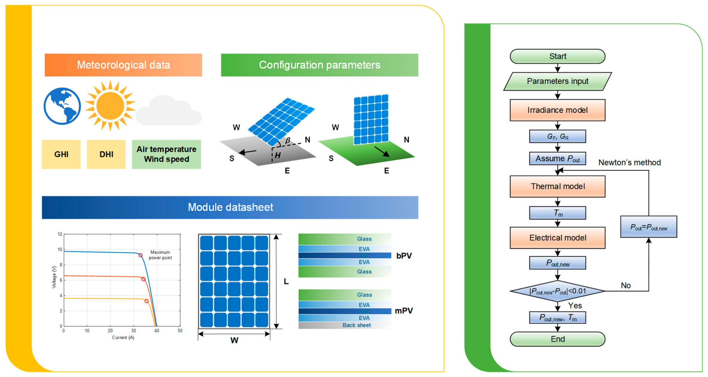
MATLAB (version 2016b) was used to implement and solve the coupled model. Figure 3 summarizes the calculation procedure. Meteorological data, installation parameters, and module datasheet information were first supplied as inputs. The irradiance model then calculated the front- and rear-side irradiance for mPV and bPV modules. Because electrical output and module temperature influence each other, the thermal and electrical equations were solved iteratively; Newton’s method converged within only a few iterations for each time step. For annual prediction, typical meteorological year data were used, and the annual performance indicators were accumulated from the time step results. The key differences between mPV and bPV modelling are absorbed irradiance and bifaciality, which affect power output and module temperature. The module specifications are listed in

Table 1. Specifications of the PV modules used in this study. The data are collected from the manufacturer.

Specification	Bifacial Module	Monofacial Module
Dimensions (mm × mm × mm)	1676 × 994 × 6	1650 × 991 × 35
Number of cells	60 (6 × 10)	60 (6 × 10)
Maximum power (W)	320	320
Open circuit voltage (V)	40.79	40.80
Short circuit current (A)	10.09	10.05
Maximum voltage (V)	33.49	33.48
Maximum current (A)	9.56	9.56
Module efficiency (%)	19.2	19.6
Temperature coefficient of Pmax (%/°C)	−0.37	−0.38
Temperature coefficient of Voc (%/°C)	−0.3	−0.3
Temperature coefficient of Isc (%/°C)	0.06	0.06
NOCT (°C)	45
Bifaciality factor (%)	70 ± 5	/

.

2.5. Performance Indicators

The DC power output of mPV and bPV modules can be determined by the maximum power point using the electrical model. Then, the annual energy yield (AEY) can be calculated by totaling the DC power output for a given time step (i.e., an hour) in one year [9]:

$$\mathrm{A}\mathrm{E}\mathrm{Y}=\sum _i\left(I_{\mathrm{m}\mathrm{p}\mathrm{p},i}{V}_{\mathrm{m}\mathrm{p}\mathrm{p},i}\right)∆t$$

(23)

A bPV module can generate more power than a monofacial one and the additional energy gain of the bPV modules over the mPV one is called the bifacial gain (BG), which is calculated as [9]:

$$\mathrm{B}\mathrm{G}={\displaystyle \frac{{\mathrm{A}\mathrm{E}\mathrm{Y}}_{\mathrm{b}\mathrm{i}}-{\mathrm{A}\mathrm{E}\mathrm{Y}}_{\mathrm{m}\mathrm{o}}}{{\mathrm{A}\mathrm{E}\mathrm{Y}}_{\mathrm{m}\mathrm{o}}}}$$

(24)

where the subscripts of ‘mo’ and ‘bi’ represent the monofacial and bifacial, respectively.

The angular losses of PV modules will inevitably result in the power loss. If PV modules are installed at different orientations and tilt angles, the power loss will be different. The power loss ($\mathrm{P}\mathrm{L}$) due to angular losses is defined to evaluate the effect of angular losses on power loss of PV modules:

$$\mathrm{P}\mathrm{L}={\displaystyle \frac{P_1-P_0}{P_1}}$$

(25)

where $P_1$ is the power calculated without considering angular losses, and $P_0$ is the power calculated by considering angular losses.

3. Experimental

3.1. System Description

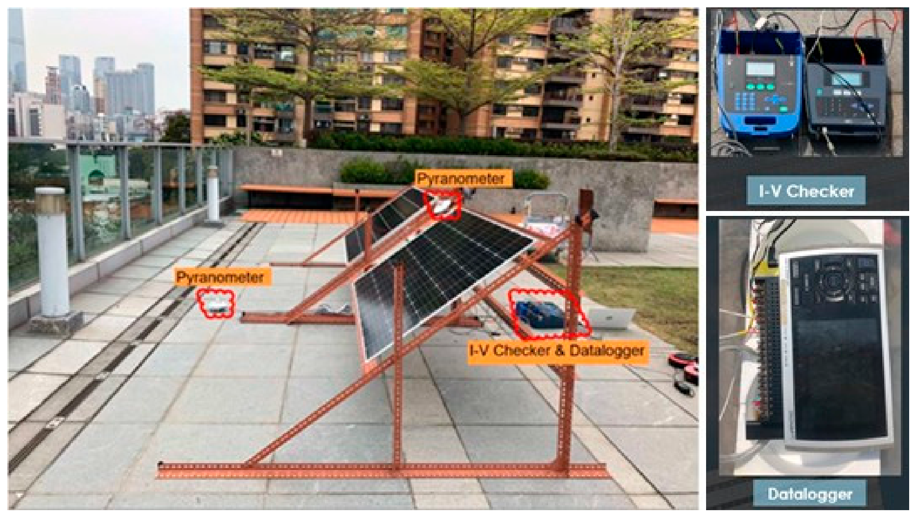
The coupled model was validated through outdoor measurements. The experimental setup for testing the bPV module is shown in Figure 4. The module was installed on an adjustable support, allowing tilt angles from 0 deg to 90 deg. Module performance was recorded using pyranometers, an I-V checker, and a data logger. Solar irradiance was measured using an MS-802 pyranometer (EKO Instruments Co., Ltd., Tokyo, Japan), with a manufacturer-specified accuracy of ±0.5% and a measurement range of 0–4000 W/m². The I–V characteristics and module power output were measured using an MP-11 I–V tracer (EKO Instruments Co., Ltd., Tokyo, Japan), which has an accuracy of ±1%, a voltage range of 10–1000 V, and a current range of 0.1–30 A. Measurements were generally recorded at 5 min intervals. Because the pyranometer arrangement did not directly provide both direct and diffuse components, an established decomposition algorithm was used to estimate them [34]. The model first calculates the clearness index and then applies piecewise correlations to determine the diffuse irradiance component. Further details of the correlations and calculation procedure are provided in the literature [34]. Four cases spanning representative tilted and vertical configurations were selected for validation, with broader seasonal validation to be considered in future long-term monitoring studies. The module specifications are listed in Table 1, and

Table 2. Configurations and weather conditions in four cases.

Case	Tilt Angle (°)	Orientation	Elevation (m)	Ground Albedo	Average Air Temperature (°C)	Average Irradiance (W/m2)
Case 1	30	South	0.25	0.1	22.5	417
Case 2	40	South	0.25	0.1	22.3	172
Case 3	90	South	0	0.1	27.7	617
Case 4	90	West	0	0.1	28.1	669

summarizes the configurations and weather conditions for the four cases.

3.2. Statistical Indexes

To quantify the accuracy of the proposed model, three different statistical indexes were adopted. The coefficient of determination, R², was used to evaluate the agreement between the measured and predicted data [26]:

$$R^2=1-{\displaystyle \frac{{\displaystyle {\sum }_{i=1}^n}{\left(y_i-f_i\right)}^2}{{\displaystyle {\sum }_{i=1}^n}{\left(y_i-\overline{y}\right)}^2}}$$

(26)

where $y_i$ and $f_i$ denote the measured and predicted values, respectively; $\overline{y}$ is the mean measured value, and $n$ is the number of data points.

The mean bias error (MBE) was used to quantify the average prediction bias [26]:

$$\mathrm{M}\mathrm{B}\mathrm{E}={\displaystyle \frac{1}{n}}{\displaystyle \sum _{i=1}^n}{\displaystyle \frac{f_i-y_i}{y_i}}$$

(27)

The normalized root mean square error (NRMSE) was calculated by scaling the root mean square error with the mean measured value [35]:

$$\mathrm{N}\mathrm{R}\mathrm{M}\mathrm{S}\mathrm{E}={\displaystyle \frac{\sqrt{\frac{1}{n}{\displaystyle {\sum }_{i=1}^n}{\left(f_i-y_i\right)}^2}}{\overline{y}}}$$

(28)

$R^2$ ranges from 0 to 1, with values above 0.7 generally indicating good predictive performance. Lower MBE and NRMSE values indicate higher model accuracy.

3.3. Model Validation

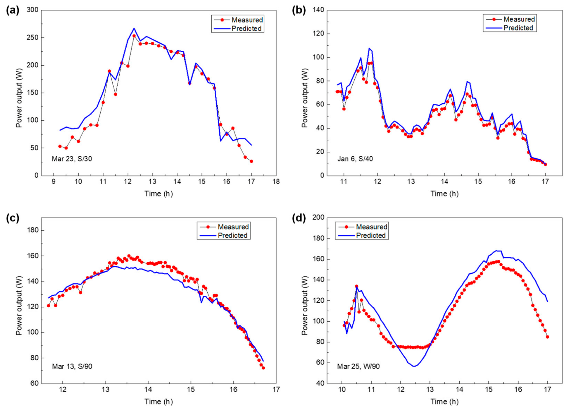
The power output predictions of the coupled model were evaluated against outdoor measurements. As shown in Figure 5, the predicted power output curves follow the measured trend reasonably well, not only for the tilted cases but also for the vertical cases. However, there are still some slight differences between the measured and predicted power output in some cases, e.g., case 1 and case 4. The differences might be caused by the nonideality of the ground (e.g., limited area for installation and changed albedo during the day), and the inaccurate estimation of DHI. Better experimental sites and measuring instruments may help reduce such errors.

Table 3. Statistical indexes calculated in four cases.

Statistical Indexes	R2	MBE	NRMSE
Case 1	0.926	−0.093	0.135
Case 2	0.920	−0.088	0.113
Case 3	0.946	0.016	0.038
Case 4	0.754	−0.035	0.124

shows the calculated statistical indexes in four cases. It is shown that $R^2$ values are between 0.754 and 0.946, $\mathrm{M}\mathrm{B}\mathrm{E}$ values are between −0.093 and 0.016, and $\mathrm{N}\mathrm{R}\mathrm{M}\mathrm{S}\mathrm{E}$ values are between 0.038 and 0.135. Good agreement was obtained between the predicted and measured power output across the four configurations. The model was subsequently applied to the comparative annual performance analysis.

4. Annual Performance Prediction

4.1. Model Comparison

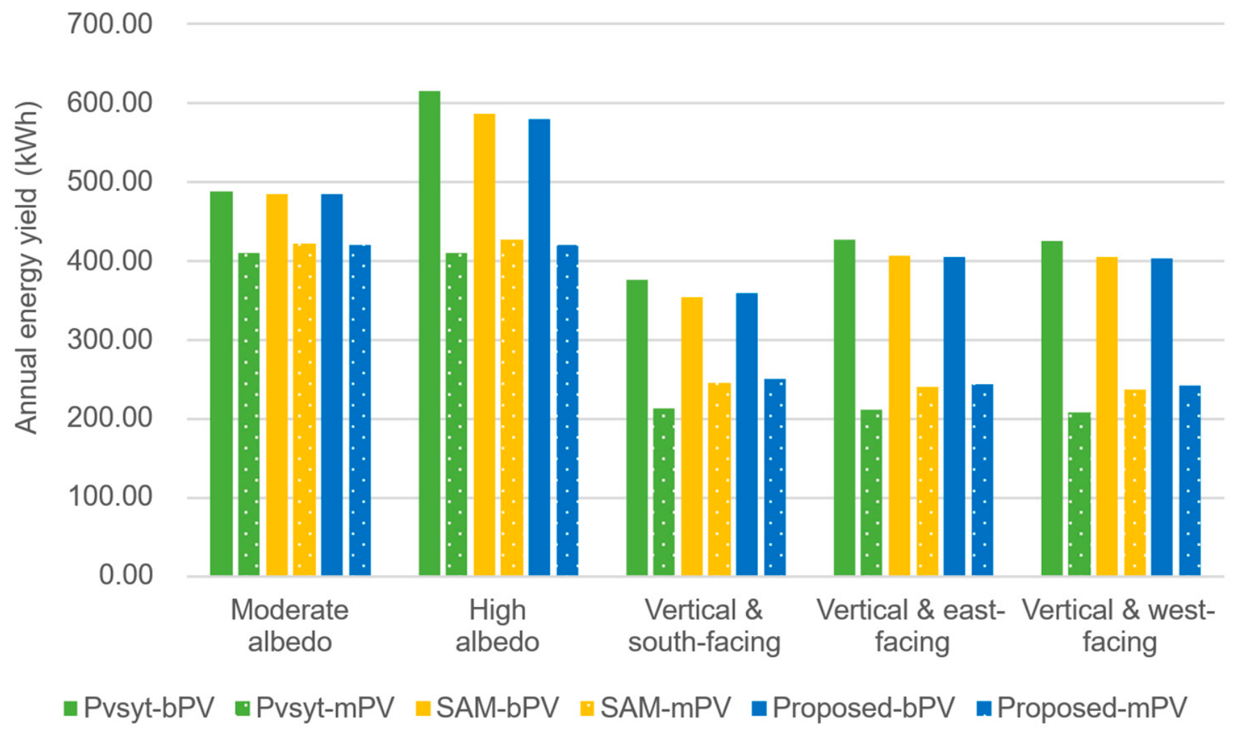
To validate the reliability of long-term performance prediction, the proposed model was compared with two of the most prestigious software, namely PVsyst (version 7.1) and System Advisor Model (SAM, version 2021.12.2). The weather data of Hong Kong was firstly obtained from Meteonorm (version 8.0), a reliable and widely used software that allows to access meteorological data around the world.

Table 4. Typical meteorological year data of Hong Kong.

Month	GHI (kWh/m2)	DHI (kWh/m2)	Ta (°C)	uw (m/s)
January	99	60	15.9	4.1
February	65	51	16.1	4.5
March	75	63	18.7	4.6
April	92	71	22.4	4.6
May	127	81	26.1	4.1
June	138	79	27.9	4.4
July	162	85	28.9	3.2
August	149	86	28.6	3.8
September	131	81	27.7	3.9
October	124	79	25.3	4.3
November	105	62	21.5	3.8
December	100	58	17.7	3.7
Total/average	1363	856	23.1	4.1

shows the TMY data of Hong Kong. Hong Kong (22.3° N, 114.2° E) has a subtropical climate, with an average annual temperature of 23.1 °C and an annual GHI of 1363 kWh/m². Then, the same meteorological data, configuration parameters, and module datasheet were input into the software and the proposed model to ensure the consistency of input data. By changing the input configuration parameters, the annual performance under varying conditions can be obtained. Five scenarios were considered to compare the results predicted by the software and the proposed model.

Table 5. The set of conditions in five scenarios for comparison.

Scenario	Description	Tilt Angle (°)	Azimuth Angle (°)	Albedo	Elevation (m)
1	Moderate albedo	20	0	0.3	1
2	High albedo	20	0	0.8	1
3	Vertical & south-facing	90	0	0.3	1
4	Vertical & east-facing	90	−90	0.3	1
5	Vertical & west-facing	90	90	0.3	1

shows the set of conditions in five scenarios for comparison. In all the simulation, the power losses due to the soiling, inverter, wire, etc., are neglected.

Figure 6 compares the annual energy yield of bPV and mPV modules calculated using PVsyst, SAM, and the proposed model. To quantify the agreement, the root mean square error (RMSE) was calculated across the five scenarios, using PVsyst and SAM as separate references. For bPV modules, the RMSE values of the proposed model were 22.36 kWh relative to PVsyst and 4.02 kWh relative to SAM. For mPV modules, the corresponding RMSE values were 27.27 kWh and 4.89 kWh, respectively. Considering all 10 paired predictions, the overall RMSE was 24.93 kWh relative to PVsyst and 4.48 kWh relative to SAM, indicating closer agreement with SAM. The larger discrepancies with PVsyst, particularly under the vertical configurations in scenarios 3–5, may be related to differences in irradiance treatment among the three tools [17,36]. Overall, the proposed model produced annual energy yield predictions comparable to those obtained from established software, supporting its application to comparative annual performance assessment.

4.2. Annual Energy Yield and Bifacial Gain

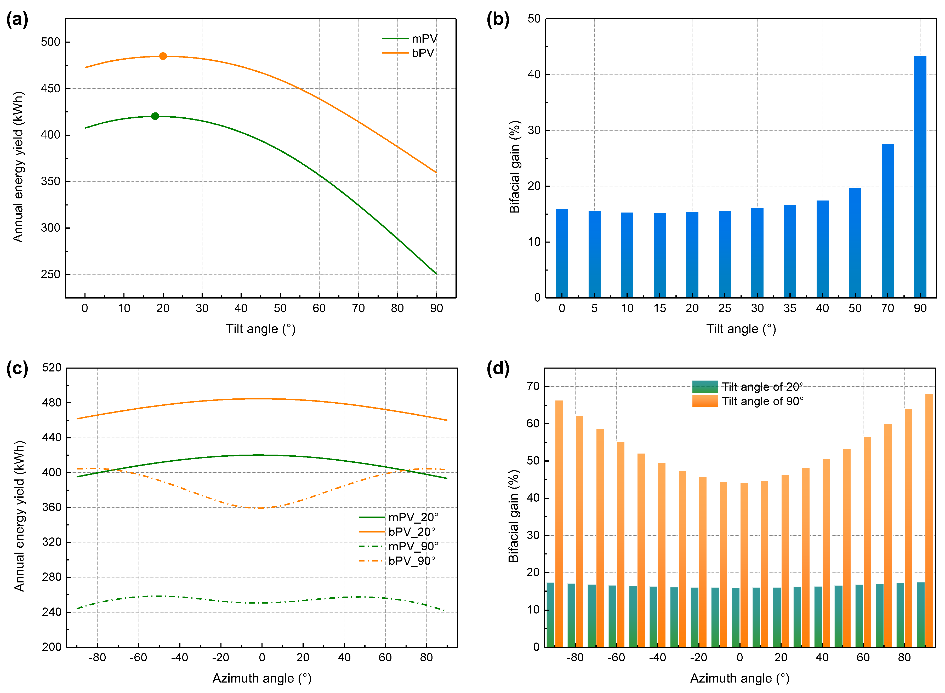
Based on the proposed model, the annual energy yield and bifacial gain of bPV modules in Hong Kong were analyzed to identify configurations suitable for land-constrained building applications. Figure 7 shows the effects of tilt angle and azimuth angle on annual energy yield and bifacial gain. As shown in Figure 7a, the annual energy yield of both south-facing mPV and bPV modules first increases and then decreases with tilt angle, with peak values of 484.7 and 420.1 kWh (i.e., 1514.7 and 1312.9 kWh/kWp), respectively. The annual optimum tilt angle is about 18 deg for mPV modules and about 20 deg for bPV modules. These values are consistent with the small optimum tilt range reported for Hong Kong and similar low-latitude locations [37,38,39], although exact values may vary with meteorological data and modelling assumptions.

Figure 7b shows that the annual bifacial gain increases from 16.0% to 43.5% when the module tilt angle increases from horizontal to vertical. Figure 7c further shows that the maximum annual energy yield of both mPV and bPV modules occurs at a tilt angle of 20 deg and a south-facing orientation. However, for vertical configurations, the optimum orientation changes: vertical bPV modules perform best when facing east or west, while vertical mPV modules perform best when facing southeast or southwest. The annual energy yield of vertically mounted bPV modules is 359.5–404.5 kWh and can reach 96.3% of that of optimally configured mPV modules (420.1 kWh at an 18 deg tilt angle and south-facing orientation). As shown in Figure 7d, when modules are installed at a 20 deg tilt angle, the annual bifacial gain is around 16% and changes only slightly with azimuth angle. In contrast, the annual bifacial gain of vertical bPV modules exceeds 43.5% and reaches a maximum of 67.2% for the west-facing configuration.

These results are important for building and urban PV applications. Although a conventional low-tilt south-facing configuration provides the highest annual energy yield, it requires horizontal or inclined surface area that may be scarce in dense cities. The vertical west-facing bPV configuration produces slightly less annual energy than the optimum mPV configuration, but it uses a vertical form that is more compatible with facades, balustrades, barriers, and other building or urban infrastructure surfaces [40,41]. Therefore, vertical bPV modules can provide a practical option for expanding PV deployment in Hong Kong and other land-constrained cities without relying only on roof or ground area.

Although the quantitative results are specific to Hong Kong, some qualitative trends may extend to other climates. Vertical bPV configurations may benefit from high diffuse irradiance, low solar elevations, or reflective surroundings, including snow-covered surfaces. In clear, low-latitude climates, however, optimally tilted modules may maintain a greater energy yield advantage. Therefore, the optimum orientation and relative performance should be recalculated using local solar geometry, diffuse fraction, ground reflectance, and ambient temperature.

4.3. Module Temperature

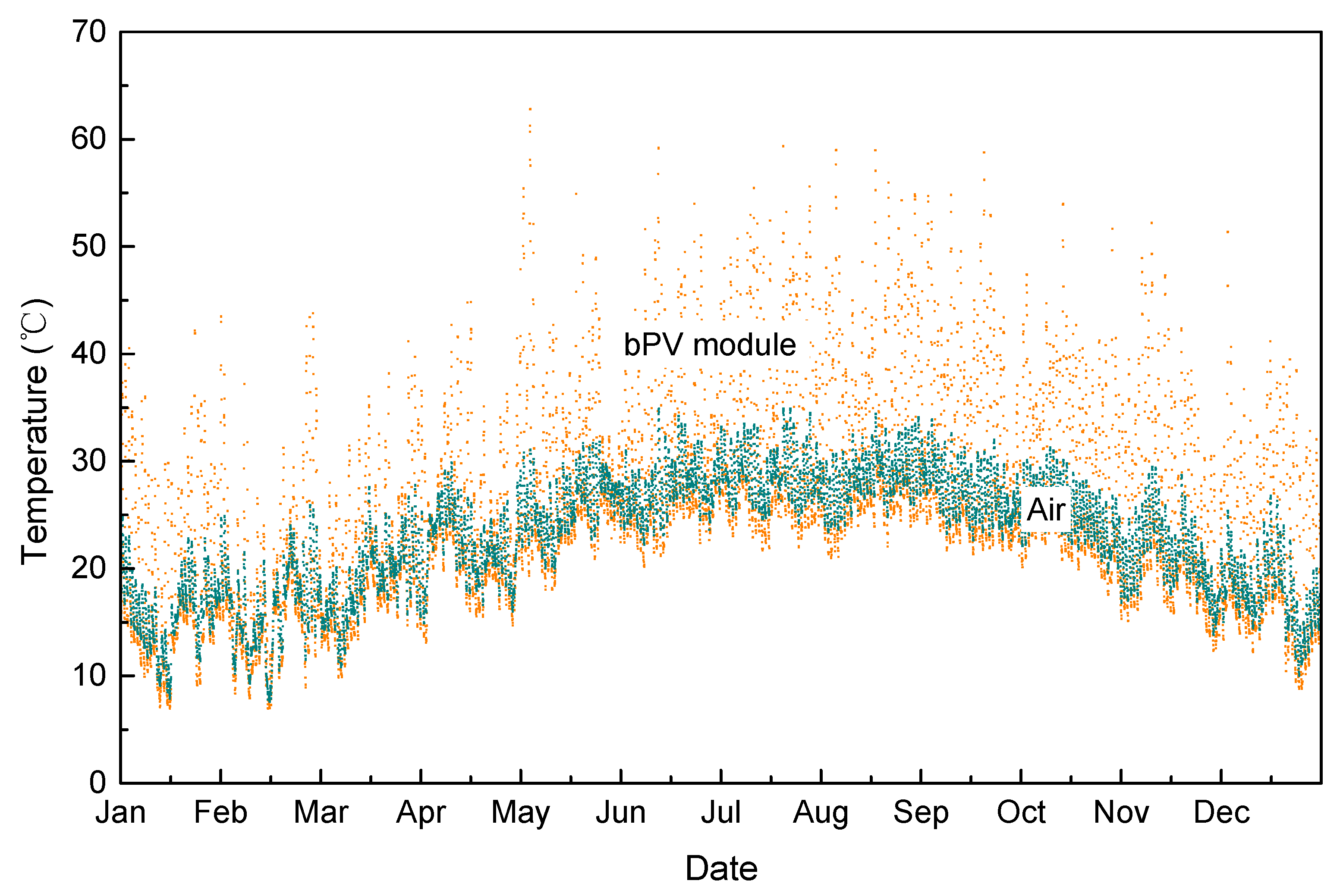
The annual temperature profile of optimally configured (south-facing and 20° tilt angle) bPV modules in Hong Kong is presented in Figure 8. It can be found that the module temperature is mostly higher than the ambient temperature during the daytime. The module temperature can reach as high as 65.4 °C in summer, about 34.7 °C higher than the ambient temperature. The high temperature would result in a significant decrease in power conversion efficiency of the module. Thus, both active and passive cooling techniques such as the air-based cooling [42] and enhanced radiative sky cooling [43,44] were studied to cool down the module and increase its power output. Based on the heat transfer model, it is also possible to calculate the module temperature when there is no solar irradiance, i.e., during the nighttime. The module temperature can be 0.8–4.8 °C lower than the ambient temperature at night due to the radiative sky cooling effect. The nighttime temperature reduction results from net long-wave radiative heat exchange with the sky, whose effective temperature is generally below the ambient air temperature. Although this cooling does not directly contribute to electricity generation, it may influence module thermal cycling, condensation risk, and the initial temperature after sunrise. Its magnitude depends on cloud cover, atmospheric humidity, wind conditions, and sky-view obstruction. Therefore, the predicted nighttime temperature reduction of 0.8–4.8 °C should be interpreted within the steady-state assumptions and requires further experimental verification.

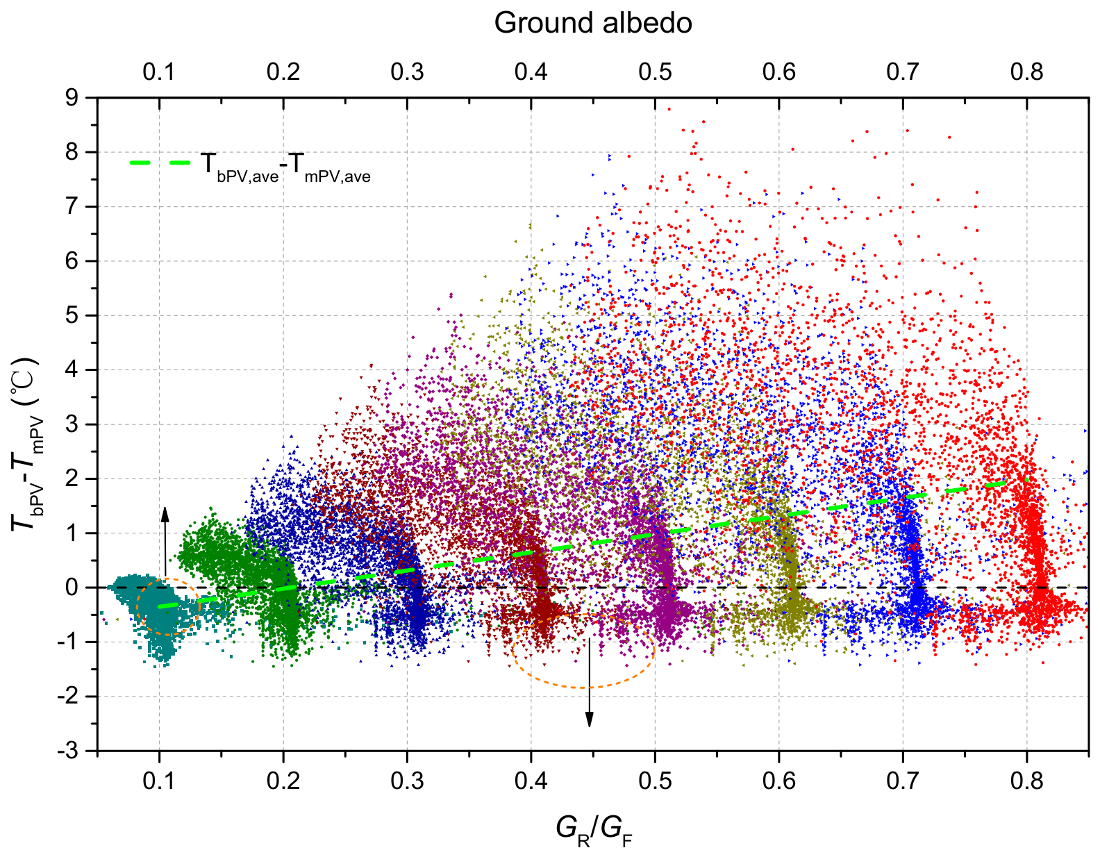
Moreover, the module temperature was compared between mPV and bPV modules. To demonstrate the effect of rear-side irradiance on the module temperature, scenarios with different ground albedos ranging from 0.1 to 0.8 were considered. Figure 9 shows the temperature difference between bPV and mPV modules. When the ratio of rear-side irradiance to front-side irradiance is lower than 0.1, the bPV module temperature is about 0.35 °C lower than the mPV module temperature. As the rear irradiance fraction increases, e.g., at higher ground albedos, the bPV module becomes hotter due to the absorption of more rear irradiance. The annual average temperature of bPV modules is almost equal to that of mPV modules at a moderate ground albedo of 0.2, and about 1.98 °C higher than mPV modules at a high ground albedo of 0.8 (also see Figure 9). Nevertheless, the benefit of increasing the ground albedo heavily covers the power loss due to the temperature rise, especially for modules with a high bifaciality factor [29]. Thus, a higher ground albedo is recommended to fully realize the potential of bPV modules.

The analysis in this part shows the unique features of the proposed thermal model as compared with those simple ones. For instance, the mechanisms of radiative and convective heat transfer and the different characteristics of the modules can be well reflected in the proposed model. Overall, the proposed thermal model provides a physically based and computationally efficient estimate of module temperature for hourly and annual performance analyses under the stated steady-state assumptions. Because module temperature was not independently validated during the experimental campaign, the absolute temperature predictions should be interpreted within these assumptions.

4.4. Annual Power Loss Due to Angular Losses

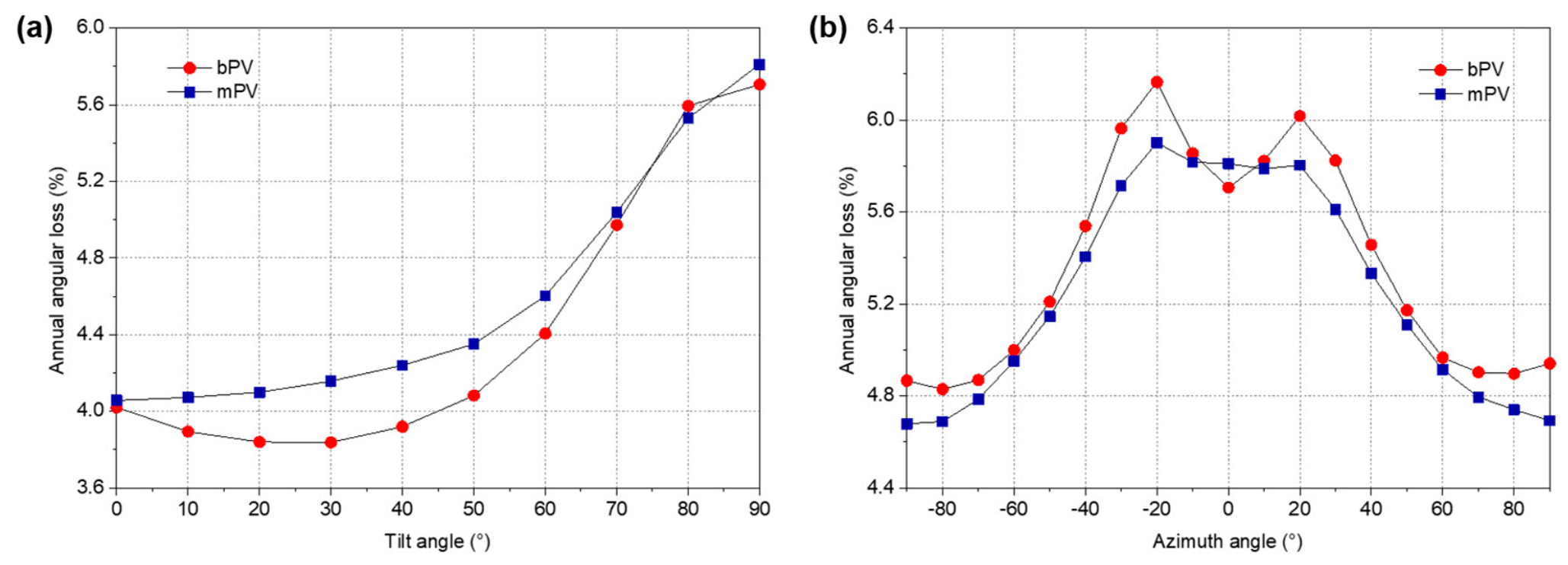
The annual power loss of bPV and mPV modules due to angular losses was analyzed, and the results are presented in Figure 10. As shown in Figure 10a, a higher tilt angle generally results in a higher annual power loss for both bPV and mPV modules, ranging from 3.84% to 5.81%. As shown in Figure 10b, the annual power loss reaches around 6% when the azimuth angle is −20 deg or 20 deg, while it decreases to around 4.8% when the azimuth angle is −90 deg or 90 deg. Overall, the annual power loss of mPV modules is slightly lower than that of bPV modules because rear-side irradiance contributes additional angular loss pathways.

For building-related deployment, the angular loss result is encouraging because the vertical east- and west-facing bPV configurations maintain relatively low annual power losses of about 4.8–4.9%. This means that the vertical configuration identified in Section 4.2 does not achieve its high bifacial gain at the expense of excessive optical angular losses. Therefore, vertical bPV modules can remain competitive in dense built environments where available facade, barrier, or envelope surfaces may not follow the conventional optimum tilt and orientation.

4.5. Implications for Building-Integrated and Building-Applied PV

The above results indicate that vertical bPV modules can help expand building-integrated and building-applied PV deployment in land-constrained urban environments. The optimum low-tilt bPV configuration provides the highest module-level annual energy yield, but such a configuration may be difficult to implement at large scale in compact cities where roof and ground areas are limited. In contrast, the vertical west-facing bPV configuration reaches 96.3% of the annual energy yield of optimally configured mPV modules, while achieving a bifacial gain of 67.2% and maintaining a relatively low angular-loss-related power loss of 4.8%. This performance makes vertical bPV modules suitable for facades, balustrades, building-attached PV systems, noise barriers, fences, and other vertical surfaces associated with buildings and urban infrastructure.

The temperature results are also relevant to building applications. At low ground albedo, optimally configured bPV modules can operate at a slightly lower annual average temperature than mPV modules, while high-albedo surroundings increase rear-side irradiance and may raise module temperature. For building design, this suggests that reflective ground or envelope materials can improve bPV irradiance gain, but their thermal effect should also be considered. The coupled model is therefore useful because it evaluates irradiance gain, temperature response, and electrical output within the same calculation framework.

This study remains a module-level analysis. In real buildings and urban districts, additional factors such as mutual shading, facade geometry, surrounding obstruction, row-to-row spacing, local wind conditions, ground reflectance heterogeneity, and mounting details can affect bPV performance. These factors should be considered in future array-level and building-level modelling. Furthermore, the experimental validation was limited to power output under four representative configurations. The uncertainty associated with the empirical DHI decomposition used in the experimental validation was not formally propagated and may contribute to the differences between predicted and measured power output. Future studies should incorporate seasonally distributed and synchronized measurements of irradiance, module temperature, and electrical output to evaluate the model over a wider range of operating conditions. Although economic performance was not evaluated in this study, vertical bPV may benefit from using otherwise inactive surfaces and, in some applications, replacing conventional building elements. These potential benefits must be balanced against additional module, mounting, structural integration, and maintenance costs. Future work should combine the predicted energy yield with project-specific cost and tariff data to assess levelized cost and payback period. Nevertheless, the present results provide a physically interpretable basis for assessing the energy performance potential of vertical bPV as a complement to conventional rooftop PV systems in dense cities.

5. Conclusions

This study developed a coupled irradiance, electrical, and thermal model for evaluating the energy performance of bPV modules in land-constrained urban building applications. The model integrates anisotropic irradiance calculation, steady-state heat transfer, and a five-parameter electrical model, and it was applied to assess tilted and vertical bPV configurations in Hong Kong. The main conclusions are as follows:

(1)

The irradiance calculation resolves beam, diffuse, and ground-reflected components on both module sides. This two-sided treatment is important for vertical east- and west-facing layouts because the module shadow can shift between the two sides during the day and alter the front/rear irradiance balance.

(2)

The coupled thermal and electrical model captures the effects of irradiance, module temperature, and angular losses on power generation. The predicted power output agreed well with outdoor measurements across the four validation configurations, supporting its use for comparative energy performance analysis.

(3)

For Hong Kong, the optimum tilt angle was about 20 deg for bPV modules and about 18 deg for mPV modules. The annual average temperature of optimally configured bPV modules was lower than that of mPV modules when the ground albedo was below 0.2, indicating that bPV modules do not necessarily suffer from a higher operating temperature under moderate albedo urban conditions. This finding also indicates that the installation angle and surrounding surface reflectance should be considered together in building-related bPV design.

(4)

The vertical west-facing bPV configuration showed strong potential for dense urban building applications. Its annual energy yield reached 96.3% of that of optimally configured mPV modules, while achieving an annual bifacial gain of 67.2% and an angular-loss-related power loss of only 4.8%. Although this configuration did not exceed the maximum yield of optimally tilted mPV, it retained comparable performance while utilizing vertical surfaces unsuitable for conventional tilted installations. It can therefore expand the total area available for PV deployment on facades, balustrades, noise barriers, fences, and other urban infrastructure.

From an engineering perspective, vertical bPV should be regarded as a complement to conventional rooftop PV rather than simply as a lower-yield alternative to optimally tilted modules. Its principal advantage is the ability to convert otherwise unused vertical surfaces into electricity-generating areas in dense cities. The proposed framework can support preliminary decisions concerning module orientation, mounting configuration, surrounding reflectance, and expected thermal performance. Potential future applications include climate-specific configuration optimization and the assessment of facade-, balustrade-, barrier-, and building-scale bPV systems. Future work should extend the analysis to other climatic regions and incorporate urban obstruction, mutual shading, facade geometry, local wind conditions, spatially varying reflectance, system losses, long-term temperature validation, and project-specific economic performance.

References

1. Kazemian, A.; Xiang, C. Large-scale analysis of photovoltaic, photovoltaic-thermal, and solar thermal systems in high-density urban environments. Appl. Energy 2025, 401, 126765. [Google Scholar] [CrossRef] [Scilit]
2. Kong, J.; Dong, Y.; Poshnath, A.; Rismanchi, B.; Yap, P.S. Application of Building Integrated Photovoltaic (BIPV) in Net-Zero Energy Buildings (NZEBs). Energies 2023, 16, 6401. [Google Scholar] [CrossRef] [Scilit]
3. Sun, B.; Lu, L.; Chen, J.; Ma, T.; Yuan, Y. Full-spectrum radiative cooling for enhanced thermal and electrical performance of bifacial solar photovoltaic modules: A nationwide quantitative analysis. Appl. Energy 2024, 362, 123037. [Google Scholar] [CrossRef] [Scilit]
4. Mahim, T.M.; Rahim, A.H.M.A.; Rahman, M.M. Review of mono-and bifacial photovoltaic technologies: A comparative study. IEEE J. Photovolt. 2024, 14, 375–396. [Google Scholar] [CrossRef] [Scilit]
5. Sun, B.; Lu, L.; Yuan, Y.; Ocłoń, P. Development and validation of a concise and anisotropic irradiance model for bifacial photovoltaic modules. Renew. Energy 2023, 209, 442–452. [Google Scholar] [CrossRef] [Scilit]
6. Zhong, J.; Zhang, W.; Xie, L.; Zhao, O.; Wu, X.; Zeng, X.; Guo, J. Development and challenges of bifacial photovoltaic technology and application in buildings: A review. Renew. Sustain. Energy Rev. 2023, 187, 113706. [Google Scholar] [CrossRef] [Scilit]
7. Gu, W.; Ma, T.; Ahmed, S.; Zhang, Y.; Peng, J. A comprehensive review and outlook of bifacial photovoltaic (bPV) technology. Energy Convers. Manag. 2020, 223, 113283. [Google Scholar] [CrossRef] [Scilit]
8. Sun, B.; Lu, L.; Lyu, N. Vertical bifacial solar photovoltaic balustrades for low-carbon buildings: A numerical analysis of energy performance. Renew. Energy 2026, 256, 124027. [Google Scholar] [CrossRef] [Scilit]
9. Liang, T.S.; Pravettoni, M.; Deline, C.; Stein, J.S.; Kopecek, R.; Singh, J.P.; Luo, W.; Wang, Y.; Aberle, A.G.; Khoo, Y.S. A review of crystalline silicon bifacial photovoltaic performance characterisation and simulation. Energy Environ. Sci. 2019, 12, 116–148. [Google Scholar] [CrossRef] [Scilit]
10. Guo, S.; Walsh, T.M.; Peters, M. Vertically mounted bifacial photovoltaic modules: A global analysis. Energy 2013, 61, 447–454. [Google Scholar] [CrossRef] [Scilit]
11. Sun, X.; Khan, M.R.; Deline, C.; Alam, M.A. Optimization and performance of bifacial solar modules: A global perspective. Appl. Energy 2018, 212, 1601–1610. [Google Scholar] [CrossRef] [Scilit]
12. Rodríguez-Gallegos, C.D.; Bieri, M.; Gandhi, O.; Singh, J.P.; Reindl, T.; Panda, S. Monofacial vs bifacial Si-based PV modules: Which one is more cost-effective. Sol. Energy 2018, 176, 412–438. [Google Scholar] [CrossRef] [Scilit]
13. Rodríguez-Gallegos, C.D.; Liu, H.; Gandhi, O.; Singh, J.P.; Krishnamurthy, V.; Kumar, A.; Stein, J.S.; Wang, S.; Li, L.; Reindl, T.; et al. Global Techno-Economic Performance of Bifacial and Tracking Photovoltaic Systems. Joule 2020, 4, 1514–1541. [Google Scholar] [CrossRef] [Scilit]
14. Gu, W.; Ma, T.; Li, M.; Shen, L.; Zhang, Y. A coupled optical-electrical-thermal model of the bifacial photovoltaic module. Appl. Energy 2020, 258, 114075. [Google Scholar] [CrossRef] [Scilit]
15. Yusufoglu, U.A.; Pletzer, T.M.; Koduvelikulathu, L.J.; Comparotto, C.; Kopecek, R.; Kurz, H. Analysis of the Annual Performance of Bifacial Modules and Optimization Methods. IEEE J. Photovolt. 2015, 5, 320–328. [Google Scholar] [CrossRef] [Scilit]
16. Appelbaum, J. The role of view factors in solar photovoltaic fields. Renew. Sustain. Energy Rev. 2018, 81, 161–171. [Google Scholar] [CrossRef] [Scilit]
17. Marion, B.; MacAlpine, S.; Deline, C.; Asgharzadeh, A.; Toor, F.; Riley, D.; Stein, J.; Hansen, C. A Practical Irradiance Model for Bifacial PV Modules. In 2017 IEEE 44th Photovoltaic Specialist Conference (PVSC); IEEE: Washington, DC, USA, 2017; pp. 1537–1542. [Google Scholar]
18. Koehl, M.; Heck, M.; Wiesmeier, S.; Wirth, J. Modeling of the nominal operating cell temperature based on outdoor weathering. Sol. Energy Mater. Sol. Cells 2011, 95, 1638–1646. [Google Scholar] [CrossRef] [Scilit]
19. Reda, I.; Andreas, A. Solar Position Algorithm for Solar Radiation Applications (Revised); National Renewable Energy Laboratory: Golden, CO, USA, 2008. [Google Scholar]
20. Noorian, A.M.; Moradi, I.; Kamali, G.A. Evaluation of 12 models to estimate hourly diffuse irradiation on inclined surfaces. Renew. Energy 2008, 33, 1406–1412. [Google Scholar] [CrossRef] [Scilit]
21. Perez, R.; Ineichen, P.; Seals, R.; Michalsky, J.; Stewart, R. Modeling daylight availability and irradiance components from direct and global irradiance. Sol. Energy 1990, 44, 271–289. [Google Scholar] [CrossRef] [Scilit]
22. Yang, D. Solar radiation on inclined surfaces: Corrections and benchmarks. Sol. Energy 2016, 136, 288–302. [Google Scholar] [CrossRef] [Scilit]
23. Hottel, H.C.; Sarofim, A.F. Radiative Transfer; McGraw-Hill: New York, NY, USA, 1967. [Google Scholar]
24. Martín, N.; Ruiz, J.M. Annual angular reflection losses in PV modules. Prog. Photovolt. Res. Appl. 2005, 13, 75–84. [Google Scholar]
25. Martin, N.; Ruiz, J. Calculation of the PV modules angular losses under field conditions by means of an analytical model. Sol. Energy Mater. Sol. Cells 2001, 70, 25–38. [Google Scholar] [CrossRef] [Scilit]
26. Ma, T.; Yang, H.; Lu, L. Solar photovoltaic system modelling and performance prediction. Renew. Sustain. Energy Rev. 2014, 36, 304–315. [Google Scholar] [CrossRef] [Scilit]
27. Jones, A.D.; Underwood, C.P. A thermal model for photovoltaic systems. Sol. Energy 2001, 70, 349–359. [Google Scholar] [CrossRef] [Scilit]
28. Lamers, M.; Özkalay, E.; Gali, R.S.R.; Janssen, G.J.M.; Weeber, A.W.; Romijn, I.G.; van Aken, B.B. Temperature effects of bifacial modules: Hotter or cooler? Sol. Energy Mater. Sol. Cells 2018, 185, 192–197. [Google Scholar] [CrossRef] [Scilit]
29. Zhang, Z.; Wu, M.; Lu, Y.; Xu, C.; Wang, L.; Hu, Y.; Zhang, F. The mathematical and experimental analysis on the steady-state operating temperature of bifacial photovoltaic modules. Renew. Energy 2020, 155, 658–668. [Google Scholar] [CrossRef] [Scilit]
30. Evangelisti, L.; Guattari, C.; Asdrubali, F. On the sky temperature models and their influence on buildings energy performance: A critical review. Energy Build. 2019, 183, 607–625. [Google Scholar] [CrossRef] [Scilit]
31. Armstrong, S.; Hurley, W.G. A thermal model for photovoltaic panels under varying atmospheric conditions. Appl. Therm. Eng. 2010, 30, 1488–1495. [Google Scholar] [CrossRef] [Scilit]
32. Yang, H.; Zhou, W.; Lu, L.; Fang, Z. Optimal sizing method for stand-alone hybrid solar–wind system with LPSP technology by using genetic algorithm. Sol. Energy 2008, 82, 354–367. [Google Scholar] [CrossRef] [Scilit]
33. Bevilacqua, P.; Perrella, S.; Bruno, R.; Arcuri, N. An accurate thermal model for the PV electric generation prediction: Long-term validation in different climatic conditions. Renew. Energy 2021, 163, 1092–1112. [Google Scholar] [CrossRef] [Scilit]
34. Lam, J.C.; Li, D.H. Correlation between global solar radiation and its direct and diffuse components. Build. Environ. 1996, 31, 527–535. [Google Scholar] [CrossRef] [Scilit]
35. Taebi, A.; Mansy, H.A. Time-frequency distribution of seismocardiographic signals: A comparative study. Bioengineering 2017, 4, 32. [Google Scholar] [CrossRef] [Scilit] [PubMed]
36. DiOrio, N.A.; Deline, C.A. Bifacial Simulation in SAM; National Renewable Energy Laboratory: Golden, CO, USA, 2018. [Google Scholar]
37. Yang, H.; Lu, L. The Optimum Tilt Angles and Orientations of PV Claddings for Building-Integrated Photovoltaic (BIPV) Applications. J. Sol. Energy Eng. 2007, 129, 253–255. [Google Scholar]
38. Li, D.; Lam, T.; Chu, V. Relationship between the total solar radiation on tilted surfaces and the sunshine hours in Hong Kong. Sol. Energy 2008, 82, 1220–1228. [Google Scholar] [CrossRef] [Scilit]
39. Peng, J.; Lu, L. Investigation on the development potential of rooftop PV system in Hong Kong and its environmental benefits. Renew. Sustain. Energy Rev. 2013, 27, 149–162. [Google Scholar] [CrossRef] [Scilit]
40. Faturrochman, G.J.; de Jong, M.M.; Santbergen, R.; Folkerts, W.; Zeman, M.; Smets, A.H.M. Maximizing annual yield of bifacial photovoltaic noise barriers. Sol. Energy 2018, 162, 300–305. [Google Scholar] [CrossRef] [Scilit]
41. Khan, M.R.; Hanna, A.; Sun, X.; Alam, M.A. Vertical bifacial solar farms: Physics, design, and global optimization. Appl. Energy 2017, 206, 240–248. [Google Scholar] [CrossRef] [Scilit]
42. Ma, T.; Kazemian, A.; Habibollahzade, A.; Salari, A.; Gu, W.; Peng, J. A comparative study on bifacial photovoltaic/thermal modules with various cooling methods. Energy Convers. Manag. 2022, 263, 115555. [Google Scholar] [CrossRef] [Scilit]
43. Li, Z.; Ahmed, S.; Ma, T. Investigating the Effect of Radiative Cooling on the Operating Temperature of Photovoltaic Modules. Sol. RRL 2021, 5, 2000735. [Google Scholar] [CrossRef] [Scilit]
44. Ahmed, S.; Li, S.; Li, Z.; Xiao, G.; Ma, T. Enhanced radiative cooling of solar cells by integration with heat pipe. Appl. Energy 2022, 308, 118363. [Google Scholar] [CrossRef] [Scilit]
Figure 1. Schematic geometry for view factor calculation between the PV module and the ground regions with and without shading. The calculation is governed by the solar elevation angle, module tilt angle, module length, and ground clearance.
Buildings 16 03020 g001
Figure 2. Heat exchange mechanisms considered for a bifacial PV module operating outdoors.
Buildings 16 03020 g002
Figure 3. Model calculation framework: parameters input (left) and computational flow chart (right).
Buildings 16 03020 g003
Figure 4. The experimental setup of the bPV module with measuring devices.
Buildings 16 03020 g004
Figure 5. Predicted and measured power output profiles of a bPV module. (a) A 30° tilt angle and south-facing (case 1). (b) A 40° tilt angle and south-facing (case 2). (c) Vertical and south-facing (case 3). (d) Vertical and west-facing (case 4).
Buildings 16 03020 g005
Figure 6. Comparison of annual energy yield calculated using three models (PVsyst, SAM, and the proposed model).
Buildings 16 03020 g006
Figure 7. Effect of tilt angle and azimuth angle on annual energy performance. (a) Effect of tilt angle on annual energy yield. (b) Effect of tilt angle on annual bifacial gain. (c) Effect of azimuth angle on annual energy yield under tilt angles of 20° and 90°. (d) Effect of azimuth angle on annual bifacial gain under tilt angles of 20° and 90°. In all cases, the ground albedo and elevation are set to 0.3 and 1 m, respectively.
Buildings 16 03020 g007
Figure 8. The annual temperature profile of optimally configured bPV modules in Hong Kong. The bPV module temperature is shown in orange, whereas the ambient air temperature is shown in blue and is generally slightly lower. The bPV modules are facing south and have a tilt angle of 20°. The ground albedo and elevation are set to 0.3 and 1 m, respectively.
Buildings 16 03020 g008
Figure 9. The temperature difference between mPV and bPV modules under different ground albedos. The scatter points show the module temperature differences, obtained at different ground albedos as a function of the rear-to-front irradiance ratio, indicated by the lower horizontal axis. The line segments represent the mean module temperature differences at the corresponding ground albedos indicated by the upper horizontal axis. The modules are facing south at a tilt angle of 20° and an elevation of 1 m.
Buildings 16 03020 g009
Figure 10. Annual power loss of mPV and bPV modules due to angular losses. (a) Effect of tilt angle on south-facing modules. (b) Effect of azimuth angle on vertical modules. The modules have an elevation of 1 m.
Buildings 16 03020 g010