Multiobjective Optimization of Thermal Performance of Opaque Envelope Components in Heating-Dominated Residential Building Based on the Uniform Design Method

Abstract

A major challenge in the optimization of thermal performance of opaque envelope components is that the calculation workload of energy consumption simulations of full factorial combinations leads to a prohibitive increase as the factors and levels multiply. Nevertheless, a reliable method for designing calculation schemes to reduce the calculation workload without sacrificing the accuracy of the results is still lacking. Accordingly, a building energy consumption simulation scheme (BECSS) based on a uniform design method (UDM) was proposed, and its feasibility was verified. A multiobjective optimization model (MOM) with the life cycle cost (LCC) and life cycle carbon emission (LCCE) as optimization objectives was established, and it was solved using the non-dominated sorting genetic algorithm-II (NSGA-II). Furthermore, an entropy-based TOPSIS method was introduced to calculate the optimal insulation thickness (OIT) of opaque building envelopes in severe cold and cold zones. The proposed framework was demonstrated through a case study of a typical residential building in Xuzhou. Extruded polystyrene panels (XPS) were used as insulation materials, and coal-fired boiler (CFB), gas-fired boiler (GFB), and air source heat pump (ASHP) were used as heat sources. Compared with the results specified by the current energy conservation standards, the MOM could achieve a balance between energy savings and environmental benefits. The LCCs change by −3.16–11.34%; nevertheless, the thermal performance of the external wall improves by 42.32–49.31%, while that of the roof improves by 6.46–21.59%; the building energy consumption (BEC) levels and the LCCEs are reduced by 25.24–30.16% and 19.25–24.74%, respectively. The indicator weights determined via the entropy weight method underscore the necessity of incorporating environmental performance indicators in the optimization of thermal performance of opaque building envelope components.

1. Introduction

The building energy consumption (BEC) accounts for approximately 20% of the nation’s total energy consumption and contributes around 18% to its total carbon emissions in China [1]. Approximately 60% of energy consumed by buildings is used for heating and air conditioning, representing the largest share of the total BEC [2,3]. Within this, heat transfer through envelopes accounts for more than 1/3 [4]. Deficient building envelopes can significantly compromise thermal comfort and energy performance. Envelope thermal characteristics also significantly influence seasonal demand-side flexibility, which is crucial for load reduction, load shifting, and coordination with low-carbon power systems [5]. Therefore, enhancing the thermal performance of building envelopes (TPBE) is a key technical strategy for building energy efficiency.

Adding insulation layers is the primary technical approach to enhancing the TPBE. Determining the optimal insulation thickness (OIT) for opaque building envelopes is critical to building energy conservation and carbon emission reduction. Therefore, extensive research has focused on this topic; key representative studies in this area are summarized and presented in Table 1.

Based on the literature review, in optimizing the thermal performance of opaque envelope components, the main methods for calculating BEC include steady-state methods (e.g., the degree-day method) and dynamic energy simulation methods. Commonly used building energy simulation software includes DesignBuilder (DB), EnergyPlus, and TRNSYS, among others. In contrast, the dynamic simulation approaches can yield more accurate results.

While some studies have sought to determine the OIT for external walls, a growing body of research recognizes that optimizing individual building envelope components in isolation is insufficient for achieving maximum overall thermal performance, energy savings, and emission reductions. This limitation stems from the complex thermal interactions among different envelope elements. Moreover, with growing environmental awareness, multiobjective optimization that balances economic and carbon emission reduction in building envelopes is gaining increasingly greater research attention.

The optimization of thermal performance of opaque envelope components requires a comprehensive framework that balances thermal performance improvements with life-cycle cost implications and policy constraints [6]. Therefore, enhancing a building’s overall thermal performance necessitates a comprehensive multiobjective optimization approach. It must account for the interdependent effects of various envelope components, such as walls, windows, roofs, doors, and airtightness. However, the calculation workload of building energy dynamic simulations of full factorial combinations leads to a prohibitive increase as the factors and levels multiply. For instance, the combinations adopted in Refs. [7], [8], and [9] are 507, 2013, and 5000 scenarios, respectively, while the number of combinations in Ref. [10] is as high as 1.10592 × 10⁷ scenarios. A major challenge in optimizing the thermal performance of opaque envelope components is reducing the number of simulation combinations and the associated computational workload without sacrificing the accuracy of the results.

The orthogonal experimental design method provides an efficient approach for managing multi-factor, multi-level energy calculations in thermal performance optimization [11]. However, the number of levels per factor in standard orthogonal arrays is generally limited to a relatively small number (typically no more than 5) [12,13]. This limitation hinders its broader use in multiobjective thermal performance optimization.

The existing literature reveals a notable research gap in developing an efficient computational strategy that can reduce simulation effort while preserving the feasibility of results. Therefore, to address this gap, a novel building energy consumption simulation scheme (BECSS) based on the uniform design method (UDM) is proposed. The uniform design, proposed by Prof. Fang Kaitai and mathematician Academician Wang Yuan [14] in 1978, is based on the number-theoretic concept of uniform distribution. This method reduces the number of tests while ensuring reliable results. Compared to the orthogonal method, the uniform design supports more variation levels per factor, which has led to its widespread adoption in engineering [15]. The effectiveness has been demonstrated in various applications, such as those reported by Liu et al. [16] and Li et al. [17]. Calibration of building energy simulation is essential for ensuring credibility, as systematic discrepancies between simulated predictions and measured data can lead to suboptimal retrofit decisions [18]. Nevertheless, the feasibility of applying the uniform design for the development of BEC programs requires further investigation.

For a design problem with m factors, each having q levels, three commonly used experimental design approaches are full factorial design, the orthogonal design, and the uniform design. Full factorial design requires $q^m$ tests, which becomes computationally prohibitive when both m and q are large. The orthogonal design requires $q^2$ tests; although this is a substantial reduction, the number of tests still grows considerably as levels increase, and the orthogonal arrays impose strict constraints on factor-level matching. In contrast, the uniform design requires only q tests—the number of tests equals the number of levels. By maximizing the uniform scatter of experimental points across the entire design space, the uniform design captures the essential system characteristics with the fewest trials while maintaining satisfactory accuracy. This advantage is particularly significant for building envelope thermal optimization, where multiple parameters (e.g., insulation thickness, thermal conductivity, specific heat, density, window-to-wall ratio) interact nonlinearly, and each simulation based on the dynamic building energy simulation tools (e.g., DesignBuilder/DeST) is computationally expensive. Therefore, the uniform design offers an ideal balance between computational accuracy and cost.

This study aims to address this knowledge gap by assessing the feasibility of implementing a BECSS framework based on the UDM. A UDM-based BECSS was developed and validated using the literature data. A multiobjective thermal performance optimization model of opaque envelope components was then established, comprehensively considering economy and environmental protection. The optimization model was solved using non-dominated sorting genetic algorithm-II (NSGA-II), and the weights of different optimization objectives were determined through the entropy weight method (EWM). Subsequently, the TOPSIS method was employed to rank the Pareto-optimal solution set (POSS) and identify the optimal design parameters of opaque envelope components. Finally, by considering a typical residential building in Xuzhou as an example, a comprehensive comparative analysis was conducted across four methods for determining thermal performance.

Table 1. The main typical studies on the optimization of the TPBE.

Researchers	Objective	Variables and ECCS	ECCM	Algorithm	Optimization Method	Main Findings
Guo et al. [19]	LCC	EWIT (160–320 mm) and ITMA (0–150 m2) were treated as continuous variables.	EnergyPlus	GA	Maximize the life-cycle net savings	The optimal EWIT is 150 mm, and the ITMA is 12.5 m2.
Akan [20]	LCC	Correlating insulation thickness with wall U-value	Degree Day method	Derivatives	Minimum	The OIT depends on the material type and the Degree-Days
Tunçbilek et al. [21]	LCC	Energy consumption calculation for external wall insulation thicknesses (Range: 0–100 mm, Step: 1 mm)	Transient 1-D numerical simulation	Graphical method	Minimum	The OIT is particularly sensitive to the building’s operational patterns.
Rosas-Flores et al. [22]	LCC	Correlating insulation thickness with wall U-value or roof U-value	Degree Day method	Derivatives	Minimum	The OIT depends on the material type and the Degree-Days.
Acikkalp et al. [23]	The total environmental costs and economic costs.	Correlating insulation thickness with wall U-value	Degree Day method	Derivatives	Minimum	The OIT of RW is 176 mm, and that of GW is 185 mm.
Axaopoulos et al. [24]	Embedded carbon and operational carbon	Insulation thickness treated as continuous	TRNSYS	GOP	Hooke–Jeeves algorithm	The OIT depends on the orientation, wall composition, and material type.
Yu et al. [25]	LCC, life cycle primary energy consumption	Various combinations of design variables: wall/roof U-values (continuous, 0–1.0 W/(m2·K)) and window U-values (discrete)	TRNSYS	NSGA-II	Weighted sum method with equal weight	The optimization equilibrium solutions of envelope parameters vary with different cities.
Duc Long [8]	The ECL and envelope-related cost	Design variable combinations (2013 samples): UvW, UvR, SHGC, WWR.	DB	NSGA-II	The point minimizing the distance to the coordinate origin	UvW = 0.71 W/(m2⋅K), UvR = 0.74 W/(m2⋅K), SHGC = 0.82, WWR = 0.2.
Rad et al. [26]	Energy, CO2 emission and cost	Various external wall insulation thicknesses (range: from 0 to 30 cm)	EnergyPlus	graphical method	Equal-weight function of all objectives	The OIT depends on the material type.
Duan et al. [11]	TAED, APCT and AUDI	Orthogonal experimental design with 12 variables: wall U-value, roof U-value, WWR, etc.	EnergyPlus	GA	The optimal solution is discussed on a case-by-case basis.	UvW and UVR both fall within 0.1–0.5 W/(m2⋅K).
He et al. [10]	Energy, CO2 emission and cost	A total of 1.10592 × 107 design scenarios for walls, roofs, and external windows were analyzed, considering 11 design variables (material thickness and types)	The steady-state method	MOQGA	Minimizing energy consumption and costs, reducing ECEs.	The optimized design envelope configuration was determined.
Wu et al. [9]	UDI, EUI and TDTP	A total of 5000 samples were generated by combining eight design variables, including wall thickness, WWR, and others.	“Office:OpenOffice” program	Octopus	Fitness function	The values of the optimization variables are specified (e.g., wall thickness = 0.5 m).
Jin et al. [7]	thermal comfort, HEC, and cost	Various combinations with 507 samples	DB	ABCA	Solution selected based on thermal comfort, low heating load, and low costs.	UvW = 0.479 W/(m2⋅K), UvR = W/(m2⋅K).
Yao et al. [27]	BEC, AHD and ACD	Various combinations of 12 optimization variables (e.g., external wall U-value, roof U-value, etc.)	EnergyPlus	NSGA-II	POSS	The variation ranges of the optimization variables are given (e.g., UvW: 0.11–0.19 W/(m2·K), UvR: 0.14–0.17 W/(m2·K).

Note: Please see the List of Abbreviations for abbreviations used in this table.

Table 1. The main typical studies on the optimization of the TPBE.

Researchers	Objective	Variables and ECCS	ECCM	Algorithm	Optimization Method	Main Findings
Guo et al. [19]	LCC	EWIT (160–320 mm) and ITMA (0–150 m2) were treated as continuous variables.	EnergyPlus	GA	Maximize the life-cycle net savings	The optimal EWIT is 150 mm, and the ITMA is 12.5 m2.
Akan [20]	LCC	Correlating insulation thickness with wall U-value	Degree Day method	Derivatives	Minimum	The OIT depends on the material type and the Degree-Days
Tunçbilek et al. [21]	LCC	Energy consumption calculation for external wall insulation thicknesses (Range: 0–100 mm, Step: 1 mm)	Transient 1-D numerical simulation	Graphical method	Minimum	The OIT is particularly sensitive to the building’s operational patterns.
Rosas-Flores et al. [22]	LCC	Correlating insulation thickness with wall U-value or roof U-value	Degree Day method	Derivatives	Minimum	The OIT depends on the material type and the Degree-Days.
Acikkalp et al. [23]	The total environmental costs and economic costs.	Correlating insulation thickness with wall U-value	Degree Day method	Derivatives	Minimum	The OIT of RW is 176 mm, and that of GW is 185 mm.
Axaopoulos et al. [24]	Embedded carbon and operational carbon	Insulation thickness treated as continuous	TRNSYS	GOP	Hooke–Jeeves algorithm	The OIT depends on the orientation, wall composition, and material type.
Yu et al. [25]	LCC, life cycle primary energy consumption	Various combinations of design variables: wall/roof U-values (continuous, 0–1.0 W/(m2·K)) and window U-values (discrete)	TRNSYS	NSGA-II	Weighted sum method with equal weight	The optimization equilibrium solutions of envelope parameters vary with different cities.
Duc Long [8]	The ECL and envelope-related cost	Design variable combinations (2013 samples): UvW, UvR, SHGC, WWR.	DB	NSGA-II	The point minimizing the distance to the coordinate origin	UvW = 0.71 W/(m2⋅K), UvR = 0.74 W/(m2⋅K), SHGC = 0.82, WWR = 0.2.
Rad et al. [26]	Energy, CO2 emission and cost	Various external wall insulation thicknesses (range: from 0 to 30 cm)	EnergyPlus	graphical method	Equal-weight function of all objectives	The OIT depends on the material type.
Duan et al. [11]	TAED, APCT and AUDI	Orthogonal experimental design with 12 variables: wall U-value, roof U-value, WWR, etc.	EnergyPlus	GA	The optimal solution is discussed on a case-by-case basis.	UvW and UVR both fall within 0.1–0.5 W/(m2⋅K).
He et al. [10]	Energy, CO2 emission and cost	A total of 1.10592 × 107 design scenarios for walls, roofs, and external windows were analyzed, considering 11 design variables (material thickness and types)	The steady-state method	MOQGA	Minimizing energy consumption and costs, reducing ECEs.	The optimized design envelope configuration was determined.
Wu et al. [9]	UDI, EUI and TDTP	A total of 5000 samples were generated by combining eight design variables, including wall thickness, WWR, and others.	“Office:OpenOffice” program	Octopus	Fitness function	The values of the optimization variables are specified (e.g., wall thickness = 0.5 m).
Jin et al. [7]	thermal comfort, HEC, and cost	Various combinations with 507 samples	DB	ABCA	Solution selected based on thermal comfort, low heating load, and low costs.	UvW = 0.479 W/(m2⋅K), UvR = W/(m2⋅K).
Yao et al. [27]	BEC, AHD and ACD	Various combinations of 12 optimization variables (e.g., external wall U-value, roof U-value, etc.)	EnergyPlus	NSGA-II	POSS	The variation ranges of the optimization variables are given (e.g., UvW: 0.11–0.19 W/(m2·K), UvR: 0.14–0.17 W/(m2·K).

Note: Please see the List of Abbreviations for abbreviations used in this table.

2. Methodology

The proposed research framework (Figure 1) is briefly described below.

(1)

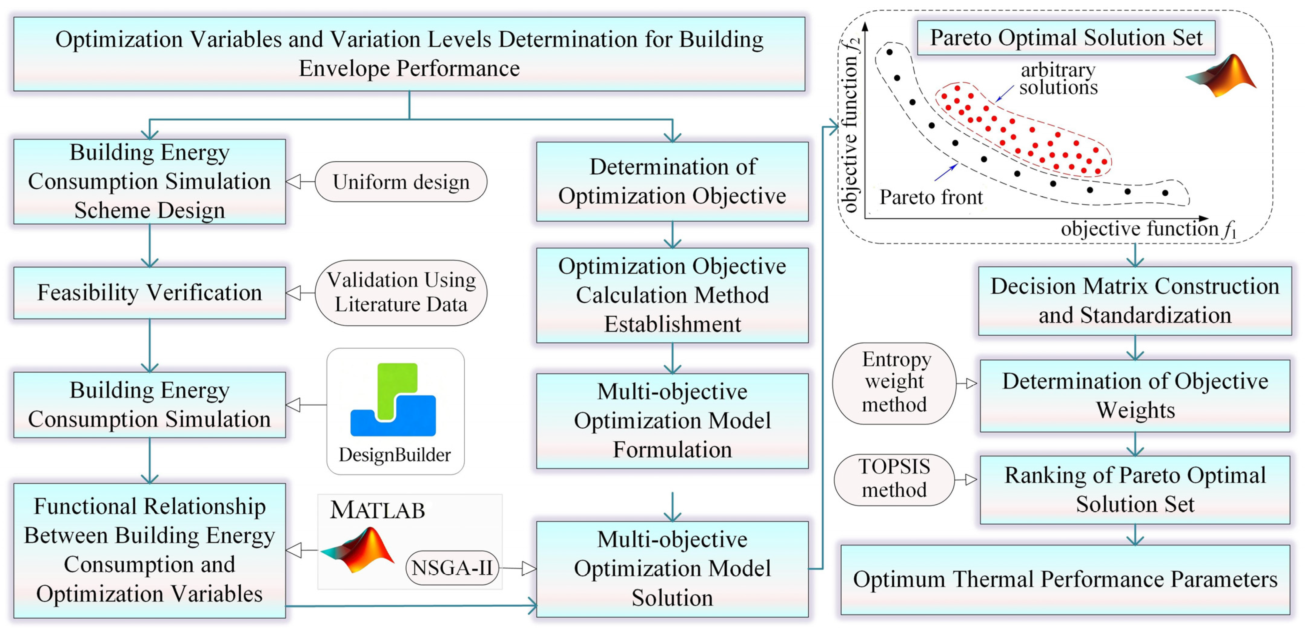
The influencing factors and variation levels for optimizing the thermal performance of opaque envelope components were determined. A BECSS was designed via a UDM, and its feasibility was verified using the literature data.

(2)

BEC simulations were then performed using DesignBuilder v6.1.0 (developed by DesignBuilder Software Ltd, Gloucestershire, UK), and the functional relationship between BEC and the optimization variables was obtained using MATLAB R2024b (developed by The MathWorks, Inc., Natick, MA, USA).

(3)

A calculation method for the life cycle cost (LCC) and life cycle carbon emission (LCCE) was proposed, and a multiobjective optimization model (MOM) of the thermal performance of opaque envelope components was established.

(4)

The optimization model was solved using NSGA-II, and the weights of each optimization objective were determined by the EWM and then integrated into the TOPSIS model. Subsequently, the optimal design parameters of thermal performance of opaque envelope components were identified by ranking the POSS.

2.1. Building Energy Consumption Simulation Scheme Based on Uniform Design

The uniform design is an experimental approach based on the uniform design table U_n (q^m), where U signifies the uniform design, n is the number of tests, m is the number of factors, and q represents the number of levels per factor. As n is much smaller than q^m, it can drastically cut down the number of tests and the associated workload. In uniform design, the uniformity is quantified by the deviation (D). A smaller D value indicates better uniformity. The following examples are used to verify the feasibility of using a UDM to develop a BECSS.

Jie et al. established a correlation equation between a building heating energy consumption (HEC) and the insulation thickness of its roof and walls by simulating 144 combinations (12 levels per factor) using DeST-h 3.0 software (developed by Department of Building Science and Technology, Tsinghua University, Beijing, China) [28]. The test involved two influencing factors: roof and external wall insulation thickness, each with 12 levels. The BECSS was designed using Column 1 and Column 5 of the uniformity design table $\mathrm{U}_{12}^{*}({12}^{10})$, and the uniformity deviation D is 0.1163. The BECs were simulated using DesignBuilder v6.1.0. A correlation was established between the building HEC and the external wall and roof insulation thickness by fitting the simulation data. Compared with the results presented in Ref. [28], the maximum error is 1.11%, with an average error of 0.46%.

Song studied the influences of the insulation thickness of the external wall and roof on the building HEC using DeST-h 3.0 [29]. The test involved two 8-level influencing factors: external wall and roof insulation thickness, with intervals of 5 mm and 10 mm, respectively. The BECSS can be designed using Column 1 and Column 3 of the uniformity design table $\mathrm{U}_8^{*}(8^5)$, and the uniformity deviation D is 0.1445. The relationship between the building HEC and the external wall and roof insulation thickness was established by fitting the data simulated using DesignBuilder v6.1.0. Compared with the results presented in Ref. [29], the maximum error is 2.99%, with an average error of 0.98%.

The above case applications demonstrate that the BECSS based on the UDM can reliably capture the impact of envelope components on the BEC. The accuracy satisfies practical engineering requirements.

Although differences in simulation software, model settings, and input parameters may introduce additional uncertainties when comparing results from DesignBuilder and DeST, it should be noted that both tools are well-established and have been extensively validated for building energy performance calculations under specific conditions. In this study, the DeST results were taken directly from the published literature, and we adopted the same building energy model and identical parameter settings to ensure consistency. The comparison was not intended to validate the absolute accuracy of either software, but rather to assess the relative effects of different insulation thickness combinations on energy consumption predictions, and to verify that the uniform-design-based simulation scheme can significantly reduce computational effort while still providing results that meet engineering accuracy requirements.

2.2. Multiobjective Optimization Model

2.2.1. The Annual Heating Energy Consumption

As specified in the Chinese code for thermal design [30], the thermal performance of opaque envelope components in severe cold and cold regions is primarily required to satisfy the insulation demands. Hence, optimizing residential envelope thermal performance based on the annual HEC is appropriate. The HEC predominantly results from transmission and ventilation heat losses. These losses are influenced by the U-values of walls, floors, and roofs, as well as the thermal performance and airtightness of windows and doors. Among these, the thermal performance of opaque envelope elements can be enhanced by increasing insulation thickness. Most heat loss occurs through walls and roofs via conduction [31], and the insulation of these opaque envelope components is therefore critical to energy performance [32]. In this context, the present paper focuses on the effect of opaque envelope insulation thickness on HEC and conducts a multiobjective optimization of this key parameter. To ensure the reliability of the optimization results, the thermal performance parameters of remaining envelope components (e.g., external windows and doors) were fixed at the limit values prescribed by the relevant energy conservation standards. This allows any variation in building energy consumption to be attributed exclusively to changes in the insulation thickness of exterior walls and roofs.

Once the opaque building envelope construction and insulation material type are determined, the annual HEC $Q_{\mathrm{H}}$ for a building with a basement becomes a function of the insulation thicknesses of the external walls, roof, and basement roof, denoted as x, y, and z, respectively. The BEC simulation can then be performed using DesignBuilder v6.1.0.

2.2.2. The Annual Heating Operating Cost

The annual heating operating cost can be calculated using Equation (1) or Equation (2), respectively.

For coal-fired boilers (CFBs) and gas-fired boilers (GFBs),

$$C_{\mathrm{H}}={\displaystyle \frac{3600Q_{\mathrm{H}}\cdot C_{\mathrm{fuel}}}{q_{\mathrm{fuel}}{\eta }_1{\eta }_2}}$$

(1)

For heat pumps,

$$C_{\mathrm{H}}={\displaystyle \frac{Q_{\mathrm{H}}\cdot C_{\mathrm{fuel}}}{SCOP}}$$

(2)

2.2.3. The Insulation Initial Investment Cost

The initial investment cost of insulation added to the external walls, roofs, and basement roofs of a building is calculated using Equation (3).

$$C_{\mathrm{ins}}=A_1\cdot \left(C_{1}x+C_{\mathrm{P}1}\right)+A_2\cdot \left(C_{2}y+C_{\mathrm{P}2}\right)+A_3\cdot \left(C_{3}z+C_{\mathrm{P}3}\right)$$

(3)

2.2.4. The Life Cycle Cost

The LCC for insulation can be calculated as follows:

$$LCC=P_1\cdot C_{\mathrm{H}}+C_{\mathrm{ins}}$$

(4)

P₁ is calculated according to Equation (5) [33].

$$P_1=PWF\left(N_{\mathrm{e}},r,d\right)={\displaystyle \sum _{j=1}^{N_{\mathrm{e}}}\frac{{\left(1+r\right)}^{j-1}}{(1+d{)}^j}=\left\{\begin{array}{l}\frac{1}{d-r}\left[1-{\left(\frac{1+r}{1+d}\right)}^{N_{\mathrm{e}}}\right],r\ne d\\ \frac{N_{\mathrm{e}}}{1+r},r=d\end{array}\right.}$$

(5)

2.2.5. The Life Cycle Carbon Emissions

The LCCEs of a building include the carbon emissions from five life-cycle stages: material production, transportation, construction, operation, and demolition. These emissions can be calculated using Equation (6), as specified in the national standard [34].

$$C_{\mathrm{C}}=C_{\mathrm{JZ}}+C_{\mathrm{M}}+C_{\mathrm{CC}}+C_{\mathrm{JC}}$$

(6)

The carbon emissions from the stages of building construction and demolition account for a small proportion of the LCCEs and can be estimated using the proportional method. Specifically, the carbon emissions from the construction period are estimated to be 4% of the total emissions from the material production period, whereas those from the demolition period are estimated to be 10% of the total emissions from the construction period [35]. The proportional estimation method used for calculating carbon emissions during the construction and demolition stages is a simplified approach. While this method is commonly adopted in early-stage evaluations lacking detailed bill-of-quantities data, its inherent shortcomings are non-negligible, particularly with respect to its limited ability to account for material-specific variations and on-site construction discrepancies.

The carbon emissions from the building operation period and material production and transportation period can be calculated using the following equation.

$$C_{\mathrm{M}}=\left[{\displaystyle \sum _{i=1}^n(E_i\cdot E{F}_i)-C_{\mathrm{P}}}\right]\cdot N_{\mathrm{e}}$$

(7)

$$C_{\mathrm{JC}}=C_{\mathrm{sc}}+C_{\mathrm{ys}}={\displaystyle {\displaystyle \sum _{i=1}^n}{M}_i{F}_i}+{\displaystyle {\displaystyle \sum _{i=1}^n}{M}_i{D}_i{T}_i}$$

(8)

$$M_i={\rho }_i{\delta }_i{A}_i/1000$$

(9)

2.2.6. The Multiobjective Optimization Model

The OIT is defined as the thickness that minimizes both LCC and LCCE, thereby providing the optimal thermal performance for an opaque building envelope. The corresponding objective function and constraints are presented in Equations (10) and (11), respectively.

$$\mathrm{Min}F(x, y, z)=\mathrm{Min}\left\{LCC(x, y, z),C_{\mathrm{C}}(x, y, z)\right\}$$

(10)

$$\mathrm{s}.\mathrm{t}.\{x_{\min }\le x\le x_{\max }, y_{\min }\le y\le y_{\max }, z_{\min }\le z\le z_{\max }\}$$

(11)

2.3. The Optimum Thermal Performance Parameters

2.3.1. The Optimization Model Solving Method

The MOM established above is a high-order multivariate nonlinear function, making it difficult to solve directly. The multiobjective genetic algorithm NSGA-II addresses this challenge effectively. It enhances the standard genetic algorithm by incorporating fast non-dominated sorting, crowding distance sorting, and an elite strategy. NSGA-II is well known for its efficiency in solving nonlinear optimization problems [36]. Therefore, the MOM in Equation (10) was solved using NSGA-II.

2.3.2. Determination of the Optimal Solution

The multiobjective genetic algorithm NSGA-II solves the objective function to obtain the POSS. The entropy-weighted TOPSIS method is employed to identify the optimal solution from this set. The TOPSIS simultaneously considers the distances to both the positive ideal solution (PIS) and the negative ideal solution (NIS). The relative closeness is between 0 and 1. The calculation process [37] is as follows, and the preference order is ranked on account of their relative closeness.

(1)

Construct the initial matrix R = [f_ij]_m×n

There are m decision alternatives {S₁, S₂, S₃, …, S_m} and n evaluation indices {I₁, I₂, I₃, … I_n}, and the attribute value that indicates the performance of each alternative with respect to the evaluation index I_j is f_ij, 1 ≤ i ≤ m, 1 ≤ j ≤ n.

(2)

Data standardization: the LCC and LCCE are negative indicators that are standardized according to Equation (12).

$$a_{ij}={\displaystyle \frac{\max (f_j)-f_{ij}}{\max (f_j)-\min (f_j)}}\hspace{1em}$$

(12)

(3)

Characteristic weight $s_{ij}$

$$s_{ij}={\displaystyle \frac{a_{ij}}{{{\displaystyle \sum }}_{i=1}^m{a}_{ij}}}$$

(13)

(4)

Entropy value of each indicator $E_j$ and weight of each indicator $w_j$

$$E_j=-{\displaystyle \frac{1}{\ln m}}{{\displaystyle \sum }}_{i=1}^m{s}_{ij}\ln s_{ij}$$

(14)

$$w_j={\displaystyle \frac{1-E_j}{{{\displaystyle \sum }}_{j=1}^n(1-E_j)}}$$

(15)

(5)

Weighted decision matrix

$$Z_{ij}=w_j{a}_{ij}\hspace{1em}$$

(16)

(6)

The distance calculated between scheme S_i and the positive and negative ideal solution.

The positive and negative ideal solution are defined as Z_j⁺ = max {Z_ij| i = 1, 2, …, m } and Z_j⁻ = min {Z_ij| i = 1, 2, …, m }, respectively. The distances between the alternative S_i and the PIS and NIS are calculated via Equations (17) and (18).

$$d_i^{+}=\sqrt{{{\displaystyle \sum }}_{j=1}^n{(Z_{ij}-Z_j^{+})}^2}$$

(17)

$$d_i^{-}=\sqrt{{{\displaystyle \sum }}_{j=1}^n{(Z_{ij}-Z_j^{-})}^2}$$

(18)

(7)

Relative closeness C_i of the alternative S_i

$$C_i={\displaystyle \frac{d_i^{-}}{d_i^{-}+d_i^{+}}}$$

(19)

In the obtained POSS, the envelope insulation thickness with the closest proximity to 1 is the OIT. The corresponding thermal performance parameters are optimal.

3. Case Applications

3.1. The Example Buildings

The case study was conducted using a north–south-oriented six-story residential building in Xuzhou, China. The residential building consists of five units, with a story height of 2.8 m. The window-to-wall ratios are 0.43 for the north facade, 0.24 for the south facade, and 0.30 for other facades. The external walls are constructed using fired coal gangue perforated brick walls. The building envelope construction is detailed in

Table 2. Basic structure of the building envelope.

Envelope	Basic Structure	Area (m2)
External wall	cement mortar (20 mm) + insulation layer + fired coal gangue perforated brick wall (190 mm) + mixed mortar (20 mm)	1505.26
Roof	fine stone concrete (40 mm) + insulation layer + cement mortar (20 mm) + lightweight aggregate concrete (80 mm) + reinforced concrete (120 mm)	569.68
External window	6 mm low-E + 12A + 6 mm, heat transfer coefficient 2.6 W/(m2·K), air-tightness performance level 4, shading coefficient 0.74 (south), 0.83 (other directions)	683.01
Basement roof	cement mortar (20 mm) + expanded clay concrete (30 mm) + insulation layer + reinforced concrete (100 mm) + lime plaster mortar (10 mm)	569.68

, while Figure 2 illustrates a typical floor plan of a residential unit.

Extruded polystyrene (XPS) is selected as the insulation material for the building external wall, roof and basement roof; its density is 35 kg/m³. The thermal conductivity of materials in each envelope construction layer is shown in

Table 3. The thermal conductivity of materials in each envelope construction layer (W/(m·K)).

Material	Cement Mortar	XPS	Fired Coal Gangue Perforated Brick Wall	Mixed Mortar	Fine Stone Concrete	Lightweight Aggregate Concrete	Reinforced Concrete	Expanded Clay Concrete	Lime Plaster Mortar
Value	0.860	0.032	0.550	0.450	0.700	0.170	2.300	0.170	0.720

.

3.2. The Annual Heating Energy Consumption

3.2.1. The Building Energy Consumption Simulation Scheme

The selection of insulation thickness should comprehensively consider both safety and thermal performance. A thicker insulation layer increases structural load, thereby imposing greater demands on both design and construction. If overlooked, this can lead to service-life issues such as hollowing, cracking, and detachment. Consequently, in the optimization of the thermal performance of opaque envelope components, it is essential to appropriately define the range of insulation thickness. Moreover, the calculated optimal value should fall within the interval, rather than at its boundaries. Otherwise, the result may represent only a locally optimal solution within the given interval, potentially leading to erroneous conclusions.

The Chinese technical standard JGJ 144-2019 [38] imposes no thickness limit for lightweight insulation materials including expanded polystyrene (EPS) and XPS with densities of 18–35 kg/m³, whereas for denser materials like mineral binder and expanded polystyrene granule bonding plaster (250–350 kg/m³), the design thickness is generally capped at 100 mm. In Ref. [19] and Ref. [21], the optimization intervals for EPS insulation thickness were set as 160–320 mm and 0–100 mm, respectively. In Ref. [26], the optimization intervals for XPS, EPS, mineral wool, and rock wool ranged from 0 to 300 mm. Ref. [39] reported optimal thicknesses of 220 mm for roof insulation and 180 mm for external wall insulation using XPS. These examples indicate that the selection of insulation thickness intervals in thermal performance optimization varies considerably across studies. In accordance with national standards and findings from the literature, the test levels for the thermal insulation thicknesses are set as follows: 10–150 mm in increments of 10 mm for external wall and roof; 30–100 mm in increments of 5 mm for basement roof. These ranges are chosen to ensure that the optimal solution falls within the variable interval while reducing computational effort. The thickness test levels for the roof and walls were set separately to account for their different thermal boundary conditions, code-specified U-value targets, and fundamental structural configurations. A uniform design table $\mathrm{U}_{15}^{*}({15}^8)$ with three factors and 15 levels was employed. The BECSS was designed to select columns 1, 2, and 3 of the uniformity design, as shown in

Table 4. Energy consumption calculation scheme and the annual HEC.

Order	Factors and Levels/Insulation Thickness (mm)			QH (kWh/year)	Order	Factors and Levels/Insulation Thickness (mm)			QH (kWh/year)
	External Wall	Roof	Basement Roof			External Wall	Roof	Basement Roof
1	1 (10 mm)	3 (30 mm)	5 (50 mm)	110,709.2	9	9 (90 mm)	11 (110 mm)	13 (90 mm)	52,999.8
2	2 (20 mm)	6 (60 mm)	10 (75 mm)	91,132.6	10	10 (100 mm)	14 (140 mm)	2 (35 mm)	50,092.0
3	3 (30 mm)	9 (90 mm)	15 (100 mm)	78,799.0	11	11 (110 mm)	1 (10 mm)	7 (60 mm)	64,523.5
4	4 (40 mm)	12 (120 mm)	4 (45 mm)	70,229.0	12	12 (120 mm)	4 (40 mm)	12 (85 mm)	54,266.6
5	5 (50 mm)	15 (150 mm)	9 (70 mm)	63,965.0	13	13 (130 mm)	7 (70 mm)	1 (30 mm)	49,434.3
6	6 (60 mm)	2 (20 mm)	14 (95 mm)	72,065.2	14	14 (140 mm)	10 (100 mm)	6 (55 mm)	46,396.3
7	7 (70 mm)	5 (50 mm)	3 (40 mm)	62,539.9	15	15 (150 mm)	13 (130 mm)	11 (80 mm)	44,213.4
8	8 (80 mm)	8 (80 mm)	8 (65 mm)	56,933.0	-	-	-	-	-

, with a uniformity deviation D = 0.06655.

3.2.2. Calculation of the Annual Heating Energy Consumption

Based on the BECSS, the annual HEC was simulated using DesignBuilder v6.1.0. The indoor design temperature is 18 °C. The occupant density is 25 m² per person; the equipment and lighting power density are 3.8 W/m² and 5 W/m², respectively. The air change rate is 0.5 h⁻¹. The zone type of the staircase was selected as semi-exterior unconditioned. The occupancy, lighting, and equipment schedules are defined according to GB 55015-2021 [40], as shown in

Table 5. The occupancy schedule (%).

Spaces	Hour of Day (h)
	1	2	3	4	5	6	7	8	9	10	11	12
Bedroom	100	100	100	100	100	100	100	50	25	0	0	0
Living room	0	0	0	0	0	0	0	50	75	100	100	100
Kitchen	0	0	0	0	0	0	0	0	0	100	100	100
Bathroom	0	0	0	0	0	0	25	25	100	25	25	25
Auxiliary Room	0	0	0	0	0	10	10	10	10	10	10	10
Spaces	Hour of day (h)
	13	14	15	16	17	18	19	20	21	22	23	24
Bedroom	0	0	0	0	0	0	0	0	0	0	25	75
Living room	100	100	100	100	100	100	100	100	100	100	0	0
Kitchen	0	0	0	0	0	100	0	0	0	0	0	0
Bathroom	25	25	25	25	25	0	50	50	100	30	30	0
Auxiliary Room	10	10	10	10	10	10	10	10	10	0	0	0

,

Table 6. The equipment schedule (%).

Spaces	Hour of Day (h)
	1	2	3	4	5	6	7	8	9	10	11	12
Bedroom	0	0	0	0	0	0	7	53	100	53	53	53
Living room	7	7	7	7	7	7	7	7	7	7	7	7
Kitchen	0	0	0	0	0	0	7	7	7	100	100	100
Bathroom	0	0	0	0	0	0	0	0	0	0	0	0
Auxiliary Room	0	0	0	0	0	0	0	0	0	0	0	0
Spaces	Hour of day (h)
	13	14	15	16	17	18	19	20	21	22	23	24
Bedroom	53	53	53	53	7	30	53	77	77	100	77	30
Living room	7	7	7	7	7	53	53	53	53	100	69	7
Kitchen	100	100	100	100	100	100	7	7	7	7	25	7
Bathroom	0	0	0	0	0	0	0	0	0	0	0	0
Auxiliary Room	0	0	0	0	0	0	0	0	0	0	0	0

and

Table 7. The general lighting schedule (%).

Spaces	Hour of Day (h)
	1	2	3	4	5	6	7	8	9	10	11	12
Bedroom	0	0	0	0	0	0	100	100	100	0	0	0
Living room	0	0	0	0	0	0	0	0	0	0	0	0
Kitchen	0	0	0	0	0	0	100	100	100	100	0	0
Bathroom	0	0	0	0	0	100	100	100	100	100	0	0
Auxiliary Room	0	0	0	0	0	10	10	10	10	10	10	10
Spaces	Hour of day (h)
	13	14	15	16	17	18	19	20	21	22	23	24
Bedroom	0	0	0	0	0	0	100	100	100	100	100	0
Living room	0	0	0	100	100	100	100	100	100	100	100	0
Kitchen	0	0	0	0	0	0	100	100	100	100	100	0
Bathroom	0	0	0	0	0	100	100	100	100	100	0	0
Auxiliary Room	10	10	10	10	10	10	10	10	10	0	0	0

. The heating period extends from 15 November to 15 March of the following year, totaling 120 days. The heating system is scheduled to operate continuously (24 h per day) during the winter season. The simulation uses the built-in hourly weather data for Xuzhou City, Jiangsu Province, China (CHN_JIANSU_XUZHOU_CSWD.EPW) available in DesignBuilder as the meteorological input. The other simulation parameters are shown in

Table 8. The simulation parameters of DesignBuilder.

Simulation Parameters	Heating Setpoint Temperatures	Heating Set Back	The External Surface Coefficient of Heat Transfer	The Internal Surface Coefficient of Heat Transfer	Natural Ventilation (By Zone)	Time Steps per Hour
Value	18 °C	15 °C	23 W/(m2·K)	8.7 W/(m2·K)	0.5 ac/h	6 steps/h

.

To further verify that the BECSS based on the UDM can reliably capture the impact of envelope components on building energy consumption (BEC), we designed a comparative experiment following the simulation schemes presented in Table 4 and the largest available orthogonal array that accommodates the specified number of levels. We then conducted a comparative analysis between the uniform design and the orthogonal design schemes for building energy consumption simulation under identical conditions. The test involved three influencing factors, each with five levels: insulation thickness of the external wall, roof, and basement roof. The test levels for the thermal insulation thickness were set as follows: 10–50 mm in increments of 10 mm for both the external wall and the roof, and 30–50 mm in increments of 5 mm for the basement roof. The BECSS was designed using Columns 1, 2, and 3 of the uniform design table $\mathrm{U}_6^{*}(6^6)$, yielding a uniformity deviation D = 0.13652, while the orthogonal design adopted the L25 ($5^6$) orthogonal array. The relationship between the annual HEC and the insulation thicknesses of the external wall, roof, and basement roof was established by fitting the data simulated using DesignBuilder. The comparative results demonstrate that under all orthogonal design simulation scenarios, the maximum relative error between the uniform design and orthogonal design results is 8.52%, and the average relative error is 3.06%. These small error magnitudes confirm that the uniform design scheme achieves results consistent with those of the orthogonal design, while requiring significantly fewer simulation runs. This additional validation—involving three factors with five levels each—provides stronger evidence that the uniform design method remains reliable even when the number of design variables increases and potential nonlinear interactions among envelope parameters are present.

The annual HEC calculation values for each envelope combination are shown in Table 4.

A multivariate nonlinear equation was established by fitting the simulation data using MATLAB, as follows:

$$\begin{array}{l}Q\mathrm{H}(x,y,z)=109040+2.72x^2+1.06y^2-0.88z^2-717.59x\\ -282.54y+180.75z+0.06xy-0.54xz-0.14yz,R^2=0.988\end{array}$$

(20)

The comparison of the simulated and fitted values from Equation (20) is shown in Figure 3. The reliability of the fitting model was assessed using four metrics, R-squared (R²), root mean square error (RMSE), mean absolute error (MAE) and mean absolute percentage error (MAPE), as shown in Equations (21)–(24). Generally, a larger R² corresponds to a superior fit, whereas smaller RMSE, MAE, and MAPE values denote better model accuracy.

$$R^2=1-{\displaystyle \frac{{\displaystyle {\sum }_{j=1}^n{({Q_{\mathrm{H}}}_j^{\mathrm{cal}}-{Q_{\mathrm{H}}}_j)}^2}}{{\displaystyle {\sum }_{j=1}^n{({Q_{\mathrm{H}}}_j-\overline{Q_{\mathrm{H}}})}^2}}}$$

(21)

$$RMSE=\sqrt{{\displaystyle \frac{{\displaystyle {\sum }_{j=1}^n{({Q_{\mathrm{H}}}_j^{\mathrm{cal}}-{Q_{\mathrm{H}}}_j)}^2}}{n}}}$$

(22)

$$MAE={\displaystyle \frac{{\displaystyle {\sum }_{j=1}^n\left|{Q_{\mathrm{H}}}_j^{\mathrm{cal}}-{Q_{\mathrm{H}}}_j\right|}}{n}}$$

(23)

$$MAPE={\displaystyle \frac{100\%}{n}}{\displaystyle {\sum }_{j=1}^n\left|\frac{{Q_{\mathrm{H}}}_j^{\mathrm{cal}}-{Q_{\mathrm{H}}}_j}{{Q_{\mathrm{H}}}_j}\right|}$$

(24)

The fitted equation of Equation (20) yielded a high coefficient of determination (R² = 0.988), along with RMSE, MAE, and MAPE values of 1713.71, 1409.98, and 2.28%, respectively. These statistical metrics, together with the comparison between simulated and fitted values illustrated in Figure 3, collectively verify the high reliability and practical applicability of the fitted curve.

DesignBuilder can export the HEC of each envelope component. Across all design scenarios, the external wall, external window, roof, and basement roof contributed 16.4–44.3%, 47.2–73.1%, 2.6–18.2%, and 0.8–2.2% of the total envelope energy consumption, respectively. The basement roof accounts for only a minor fraction of the total envelope heat load, and its insulation thickness exerts a negligible influence on the overall energy performance. Therefore, its insulation level was fixed according to the requirements of the current building energy efficiency standards. This simplification reduces the computational burden of the multiobjective optimization without compromising the reliability of the optimal solutions for the external walls and roof.

3.3. The Thermal Performance Optimization of the Opaque Envelope Components

The case study considered a CFB, a GFB, and an air source heat pump (ASHP) as heat sources, and their main performance parameters are presented in Table 9. The price of XPS insulation material is 107.40 USD/m³; the parameters C_p1, C_p2, and C_p3 are 8.65, 2.51 and 9.07 USD/m², respectively. The carbon emissions factors for coal, natural gas, and electricity are 2.47 tCO₂/t [41], 55.54 tCO₂/TJ [34], and 0.7921 tCO₂/MWh [34], respectively. The carbon emissions per unit heat consumption (CEUHC) for the heat source of CFB and ASHP can be calculated using Equation (25), whereas those for the GFB heat source are determined using Equation (26):

$$CEUHC={\displaystyle \frac{E{F}_i}{q_{\mathrm{fuel}}{\eta }_1{\eta }_2}}$$

(25)

$$CEUHC={\displaystyle \frac{E{F}_i}{{\eta }_1{\eta }_2}}$$

(26)

When ASHP is used as a heat source, ${\eta }_1={SCOP}_{\mathrm{ASHP}}$. The calculation results of the CEUHC for each type of heat source are also shown in Table 9.

Table 9. Performance parameters of different heat sources.

Type of Heat Source	${\mathit{q}}_{\mathbf{fuel}}$	η1	η2	${\mathit{S}\mathit{C}\mathit{O}\mathit{P}}_{\mathbf{ASHP}}$	${\mathit{C}}_{\mathbf{fuel}}$	CEUHC (tCO2/TJ)
CFB	29,307 kJ/kg [42]	0.8 [42]	0.92 [42]	/	121.3457 USD/t [43]	114.51
GFB	35,600 kJ/m3 [42]	0.9 [42]	0.92 [42]	/	0.3808 USD/m3 [44]	67.08
ASHP	3600 kJ/kWh [42]	/	1.0	3 [42]	0.0736 USD/(kWh) [45]	73.34

Note: When ASHP is used as heat source, the room air conditioner is installed indoors, η₂ = 1.0.

Table 9. Performance parameters of different heat sources.

Type of Heat Source	${\mathit{q}}_{\mathbf{fuel}}$	η1	η2	${\mathit{S}\mathit{C}\mathit{O}\mathit{P}}_{\mathbf{ASHP}}$	${\mathit{C}}_{\mathbf{fuel}}$	CEUHC (tCO2/TJ)
CFB	29,307 kJ/kg [42]	0.8 [42]	0.92 [42]	/	121.3457 USD/t [43]	114.51
GFB	35,600 kJ/m3 [42]	0.9 [42]	0.92 [42]	/	0.3808 USD/m3 [44]	67.08
ASHP	3600 kJ/kWh [42]	/	1.0	3 [42]	0.0736 USD/(kWh) [45]	73.34

Note: When ASHP is used as heat source, the room air conditioner is installed indoors, η₂ = 1.0.

For an individual building, the carbon sink of green vegetation can be taken as 0 tCO₂/a. The other economic and carbon emission input parameters are shown in Table 10.

Unlike the 50-year service life typical of conventional buildings, the payback period for investments for thermal insulation must not exceed 10 years to be economically viable [46]. Hence, in the thermal performance optimization of opaque building envelope structures, the analysis period N_e is generally taken as 10–20 years [19,20,21,23]. In this study, a 20-year analysis period was adopted, during which the XPS insulation materials were assumed to maintain their thermal performance without replacement, consistent with the specified service life of >25 years for XPS under standard installation conditions [38]. This assumption is reasonable for the 20-year timeframe, though we acknowledge that long-term performance degradation could occur beyond this period, which should be investigated in future research.

Table 10. The economic and carbon emission input parameters.

Parameters	The Carbon Emission Factor for XPS Production Process	The Carbon Emission Factor for XPS Transportation	Di	Ne	r	d
Value	5.02 tCO2/t [34]	0.179 kgCO2/(t·km) [34]	500 km [34]	20 a	0.0197 [47]	0.042 [48]

Table 10. The economic and carbon emission input parameters.

Parameters	The Carbon Emission Factor for XPS Production Process	The Carbon Emission Factor for XPS Transportation	Di	Ne	r	d
Value	5.02 tCO2/t [34]	0.179 kgCO2/(t·km) [34]	500 km [34]	20 a	0.0197 [47]	0.042 [48]

The MOM was solved using the NSGA-II algorithm, with the maximum number of evolutionary generations set as the termination condition. The population size, elite scale, crossover probability, and mutation probability are adopted from Refs. [8,9], [25], [8,9] and [9], respectively. As for the evolutionary generation, its optimal value is problem-dependent: Ref. [25] uses 20, Ref. [8] uses 50, and Ref. [9] adopts a range of 10 to 500. In this study, building upon these references, we compare the optimization results obtained with 150 and 200 generations. The relative error between the two is less than 5.00%, indicating that the difference is negligible. Therefore, the optimization results reported in this paper are based on an evolutionary generation of 200. The selection mechanism adopts binary tournament selection (with two individuals). Uniform crossover and random resetting mutation are employed as the crossover and mutation operators [49], respectively. The elitist strategy merges the parent and offspring populations and performs truncation selection based on non-dominated sorting and crowding distance, with the elite population size set to 50. The relevant parameters are listed in

Table 11. Calculation parameters of NSGA-II.

Project Title	Population Size	Elite Scale	Crossover	Crossover Probability	Mutation	Probability of Mutation	Evolutionary Algebra
Value	100	50	Uniform	0.9	random	0.05	200

. After 10 independent runs, the best-performing set of results is selected.

During the optimization, the external wall and roof insulation thicknesses are varied within the range 10–150 mm with a step size of 1 mm. The building HEC was calculated using Equation (20), and the LCC and LCCE were obtained from Equation (4) and Equation (6), respectively.

The POSSs for different heat source types (HSTs) are obtained by implementing the genetic algorithm module in MATLAB.

The weights of LCC and LCCE are calculated using Equation (15). The relative closeness of each solution in the POSS was obtained from Equation (19). The optimal solution is identified as the one with the maximum closeness value.

4. Results and Analysis

4.1. The Methods for Determining the Insulation Thickness

The external wall and roof insulation thicknesses can be calculated using four methods, as described below:

(1)

The limit value method (LVM): This method calculates the insulation thickness based on the thermal performance limits specified in GB 55015-2021 [40]. The results are presented in

Table 12. Optimal thermal performance and corresponding economic and environmental parameters calculated by different methods.

HST	Method	External Wall		Roof		OAAHTC (W/(m2·K))	BEC (kWh)	LCC (k$)	LCCEs (tCO2)
		Insulation Thickness (mm)	U Value (W/(m2·K))	Insulation Thickness (mm)	U Value (W/(m2·K))
CFB	LVM	53	0.4489	87	0.3000	0.4285	67,219.80	58.06	583.78
	LCCM	47	0.4901	38	0.5711	0.5093	77,585.20	57.40	662.34
	LCCEM	127	0.2202	129	0.2176	0.2796	46,422.02	65.96	437.57
	MOM	122	0.2281	118	0.2352	0.2879	46,949.11	64.65	439.34
GFB	LVM	53	0.4489	87	0.3000	0.4285	67,219.80	85.86	354.21
	LCCM	96	0.2800	94	0.2856	0.3282	52,159.63	82.21	294.31
	LCCEM	125	0.2233	123	0.2269	0.2833	46,615.68	84.61	278.77
	MOM	114	0.2419	112	0.2461	0.2980	47,958.77	83.14	280.99
ASHP	LVM	53	0.4489	87	0.3000	0.4285	67,219.80	62.61	384.54
	LCCM	59	0.4140	61	0.4049	0.4302	67,959.96	62.28	387.37
	LCCEM	124	0.2249	125	0.2237	0.2835	46,639.62	68.46	299.86
	MOM	105	0.2595	96	0.2806	0.3155	50,252.99	65.01	310.51

.

(2)

The LCC Method (LCCM) and LCCE Method (LCCEM): These are single-objective optimization methods. The corresponding results are shown in Table 12.

(3)

The multiobjective optimization model (MOM): This method is proposed in Section 2. The POSSs for the three HSTs are shown in Figure 4.

The objective weights of the LCC and LCCE are 0.11 and 0.89 for CFB, 0.09 and 0.91 for GFB, and 0.08 and 0.92 for ASHP. The corresponding optimal thermal performance, economic, and environmental parameters, the U-values of the external walls and roof, and the overall area-weighted average heat transfer coefficient (OAAHTC) for each heat source type are given in Table 12. The OAAHTC is defined as the area-weighted average of local overall heat transfer coefficients over the entire heat transfer surface, which can be calculated as follows:

$$OAAHTC ={\displaystyle \frac{{\displaystyle \sum _j{U}_j{A}_j}}{{\displaystyle \sum _j{A}_j}}}$$

(27)

4.2. Discussion of the Results

The results shown in Table 12 indicate the following:

(1)

Compared with the results obtained from the LVM, the OITs of the external wall and roof determined by the LCCM are smaller when a CFB is used as the heat source; in contrast, greater insulation thicknesses are required for both opaque envelope components when GFB or ASHP systems are employed as heat sources. Moreover, the optimal U-values in these cases are lower than the maximum U-value limit prescribed for opaque building envelopes in the current energy efficiency design standards. These findings indicate that the thermal performance requirements specified in the existing energy efficiency standards still retain potential for further energy savings.

(2)

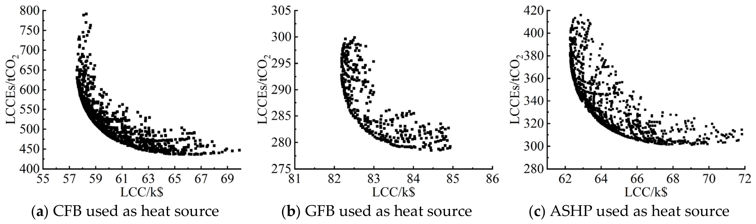
For the three HSTs of CFB, GFB, and ASHP, the OITs are applied to the external wall and roof. Under this condition, the LCCM can achieve the minimum LCCs, which are 57.40, 82.21, and 62.28 k$, respectively, while the LCCEM yields the lowest LCCEs, corresponding to 437.57, 278.77, and 299.86 tCO₂, respectively.

(3)

The MOM achieves a balance between energy savings and environmental benefits. For the three HSTs of CFB, GFB, and ASHP, although the LCCs change by 11.34%, −3.16% and 3.83%, respectively, the improvements in thermal performance, energy savings, and emission reduction are significant. Specifically, the thermal performance of the external wall is improved by 49.31%, 46.25% and 42.32%, respectively; and that of the roof by 21.59%, 17.97% and 6.46%, respectively; correspondingly, the BEC decreases by 30.16%, 28.65% and 25.24%, and the LCCEs are reduced by 24.74%, 20.67% and 19.25%, respectively.

(4)

The resulting LCCEs from the GFB and ASHP are significantly lower than those from the CFB. Moreover, the enhanced thermal performance of opaque envelope components meets the requirements of three-star green buildings, delivering substantial combined benefits in terms of economy, energy savings, and environmental protection. Therefore, transitioning the energy structure by restricting coal-fired boilers can lead to improved energy savings and environmental benefits.

(5)

The optimal OAAHTC values derived from the LCCM, LCCEM, and MOM vary with the heat source type. The OAAHTC determined by the LCCM exhibits an inverse relationship with the operating charge per unit heat consumption (OCUHC) of the heat source, meaning that it decreases as the OCUHC increases. In contrast, the OAAHTC values obtained from both the LCCEM and MOM decrease with increasing CEUHC of the heat source. For a given heat source, the LCCEM yields the smallest OAAHTC (i.e., the best thermal performance), while the LCCM results in the poorest thermal performance. The OAAHTC values obtained by the MOM lie between those derived from the other two models.

(6)

Due to their substantial weights as determined by the EWM (0.89, 0.91, and 0.92, for the CFB, GFB, and ASHP, respectively), the optimization outcomes of the LCCEM and MOM show no significant differences. The LCC indicators exhibit limited variation and thus contain less information, resulting in relatively low assigned weights. In contrast, the environmental performance indicators are essential to the thermal performance optimization process. While this outcome aligns well with China’s current carbon-focused policy agenda, it may not adequately reflect the priorities of stakeholders who must balance economic and environmental objectives.

It should be acknowledged that certain key parameters—including transport distance, service life, discount rate, construction and demolition carbon assumptions, and heat-source performance—were treated as fixed values in this study based on the best available data and relevant standards. These assumptions may introduce uncertainties that affect the absolute values of the optimization results. Therefore, the findings should be interpreted with these contextual limitations in mind.

5. Conclusions

A BECSS based on a UDM was developed and validated. The MOM for the thermal performance of opaque envelope components optimization was established and solved using the multiobjective genetic algorithm NSGA-II. Subsequently, an entropy-based TOPSIS method was employed to determine the OIT of opaque building envelopes in severe cold and cold zones. The proposed framework was demonstrated through a case study of a typical residential building in Xuzhou. The main conclusions are as follows:

(1)

The BECSS based on the UDM can significantly reduce the number of scheme combinations and the associated calculation workload while ensuring the reliability of the calculation results.

(2)

The multiobjective genetic algorithm NSGA-II was employed to solve the MOM of the thermal performance of opaque envelope components, and the entropy-weighted TOPSIS method was used to rank the POSS and identify the optimal design parameters. This approach can obtain the optimal scheme that enhances comprehensive benefits in terms of economic performance, energy savings, and environmental protection.

(3)

Compared with the LVM, the MOM achieves a more balanced trade-off between energy savings and environmental benefits. For the three HSTs of CFB, GFB, and ASHP, the LCCs vary from −3.16% to 11.34%; nevertheless, the thermal performance of the external wall and roof is improved by 42.32–49.31% and 6.46–21.59%, respectively; the BEC levels and the LCCEs are reduced by 25.24–30.16% and 19.25–24.74%, respectively.

(4)

The weights of the LCC and LCCE determined by the EWM indicate that the LCC indicators exhibit limited variation and thus receive relatively low weights. This underscores the necessity of incorporating environmental performance indicators in the thermal performance optimization.

This study proposed a new MOM of the thermal performance of opaque envelope components based on the UDM. The optimization model only considered the impact of external wall and roof insulation thickness on thermal performance. However, as the thermal performance of opaque envelope components is influenced by numerous factors, subsequent research will explore the effects of multiple factors, including window and door systems, basement roof, wall configurations, and insulation material types on envelope thermal performance. This expanded investigation aims to provide a more comprehensive understanding and to offer robust theoretical and technical support for the design of the thermal performance of opaque envelope components.

It should also be noted that the conclusions of this study are derived under specific economic and carbon emission parameters, and variations in these parameters may exert a non-negligible influence on the results. Therefore, future research should extend this work by incorporating comprehensive sensitivity and uncertainty analyses, including probabilistic approaches such as Monte Carlo simulation, to propagate input parameter uncertainties through the optimization framework. In addition, dynamic parameters—for instance, time-varying discount rates and future grid decarbonization trajectories aligned with China’s 2030/2060 carbon neutrality goals—could be integrated to further enhance the long-term reliability of the optimization outcomes. The proportional estimation method used for carbon emission calculation during the construction and demolition stages should also be refined to better capture the effects of differentiated insulation materials and construction details, varying construction techniques, and alternative demolition strategies on the life-cycle carbon emissions of buildings. Collectively, these extensions would substantially strengthen the practical applicability of the proposed BECSS methodology in real-world design practice.

References

- Building Energy Research Center of Tsinghua University. Annual Report on China Building Energy Efficiency 2025: Special Topic on Urban Residential Buildings; China Architecture & Building Press: Beijing, China, 2025. [Google Scholar]
- Jaffar Abass, P.; Muthulingam, S. Incorporation of phase change materials into building materials and envelopes for thermal comfort and energy optimization: A comprehensive review. J. Build. Eng. 2025, 103, 112106. [Google Scholar] [CrossRef] [Scilit]
- Kaynakli, O. A review of the economical and optimum thermal insulation thickness for building applications. Renew. Sustain. Energy Rev. 2012, 16, 415–425. [Google Scholar] [CrossRef] [Scilit]
- Ban, G.S. Building Envelope Energy Efficiency Design and Practice; China Architecture & Building Press: Beijing, China, 2010. [Google Scholar]
- Li, W.; Sui, W.; Cheng, L. Quantifying seasonal demand-side flexibility in residential air conditioning under diverse control strategies. Energy Build. 2026, 352, 116764. [Google Scholar] [CrossRef] [Scilit]
- Ozarisoy, B.; Altan, H. Building Performance Evaluation: Policy Design and Life-Cycle Cost Impact Analysis of Retrofit Strategies. In Handbook of Retrofitting High Density Residential Buildings; Springer: Cham, Switzerland, 2022. [Google Scholar]
- Jin, G.H.; Wei, X.; Zhang, W.J. Construction of multi-objective optimization model for energy saving of residential buildings in grassland of western Inner Mongolia. J. Shandong Agric. Univ. (Nat. Sci. Ed.) 2020, 51, 347–351. [Google Scholar]
- Duc Long, L. An AI-driven model for predicting and optimizing energy-efficient building envelopes. Alex. Eng. J. 2023, 79, 480–501. [Google Scholar] [CrossRef] [Scilit]
- Wu, H.; Zhang, T. Multi-objective optimization of energy, visual, and thermal performance for building envelopes in China’s hot summer and cold winter climate zone. J. Build. Eng. 2022, 59, 105034. [Google Scholar] [CrossRef] [Scilit]
- He, L.; Wang, W. Design optimization of public building envelope based on multi-objective quantum genetic algorithm. J. Build. Eng. 2024, 91, 109714. [Google Scholar] [CrossRef] [Scilit]
- Duan, Y.; Zhang, T.; Yang, Y. A multi-objective approach to optimizing the geometry and envelope of rural dwellings for energy demand, thermal comfort, and daylight in cold regions of China: A case study of Shandong province. Energy Convers. Manag. 2024, 322, 119128. [Google Scholar] [CrossRef] [Scilit]
- Shina, S. Industrial Design of Experiments:A Case Study Approach for Design and Process Optimization; Springer Nature: Cham, Switzerland, 2022. [Google Scholar]
- Liu, F.; Weng, M. Data-Based Experimental Design and Data Processing; Chongqing University Press: Chongqing, China, 2021. [Google Scholar]
- Fang, K.T. Uniform Design and Uniform Design Tables; Science Press: Beijing, China, 1994. [Google Scholar]
- Dong, R.; Liang, S.Y.; Qiu, L.Y. Multi-factor analysis of downwind wind loads on tall buildings across the Taiwan Strait based on uniform design. J. Tongji Univ. (Nat. Sci.) 2023, 51, 1383–1394. [Google Scholar] [CrossRef]
- Liu, H.J.; Zhang, J.L.; Dong, H.Q. Screening and validation of anti-Parkinson’s disease dose rationing based on homogeneous design of Turtle Peony and Flat Tremor Formula combined with Dobasic Hydrazide Tablets in Parkinson’s disease. Pharmacol. Clin. Chin. Mater. Medica 2020, 36, 163–168. [Google Scholar] [CrossRef]
- Li, L.; Fang, Q.; Cai, C.Y. Application of the uniform design method in the proportioning design of steel slag concrete. China Water Transp. 2021, 21, 108–109,111. [Google Scholar]
- Ozarisoy, B.; Altan, H. Energy Calibration: Developing a Novel Methodology to Calibrate Building Energy Performance of Social Housing Estates. In Handbook of Retrofitting High Density Residential Buildings; Springer: Cham, Switzerland, 2022. [Google Scholar]
- Guo, R.; Shi, D.; Liu, Y. A modeling framework for integrating model predictive control into building design optimization. Appl. Energy 2025, 388, 125686. [Google Scholar] [CrossRef] [Scilit]
- Akan, A.E. Determination and Modeling of Optimum Insulation Thickness for Thermal Insulation of Buildings in All City Centers of Turkey. Int. J. Thermophys. 2021, 42, 49. [Google Scholar] [CrossRef] [Scilit]
- Tuncbilek, E.; Komerska, A.; Arici, M. Optimisation of wall insulation thickness using energy management strategies: Intermittent versus continuous operation schedule. Sustain. Energy Technol. 2022, 49, 101778. [Google Scholar] [CrossRef] [Scilit]
- Rosas-Flores, J.A.; Rosas-Flores, D. Potential energy savings and mitigation of emissions by insulation for residential buildings in Mexico. Energy Build. 2020, 209, 109698. [Google Scholar] [CrossRef] [Scilit]
- Açıkkalp, E.; Kandemir, S.Y. A method for determining optimum insulation thickness: Combined economic and environmental method. Therm. Sci. Eng. Prog. 2019, 11, 249–253. [Google Scholar] [CrossRef] [Scilit]
- Axaopoulos, I.; Axaopoulos, P.; Gelegenis, J. Optimum external wall insulation thickness considering the annual CO2 emissions. J. Build. Phys. 2019, 42, 527–544. [Google Scholar] [CrossRef] [Scilit]
- Yu, Z.Y.; Lu, F.; Zou, Y. A Simulation-based Multi-objective Optimization Approach for Design of Nearly Zero Energy Buildings. Build. Sci. 2019, 35, 8–15. [Google Scholar] [CrossRef]
- Rad, E.A.; Fallahi, E. Optimizing the insulation thickness of external wall by a novel 3E (energy, environmental, economic) method. Constr. Build. Mater. 2019, 205, 196–212. [Google Scholar] [CrossRef] [Scilit]
- Yao, G.; Zhang, Y.; Pang, Y. Optimization of envelope design parameters for nearly zero energy retrofit of rural residence: An integrated multi-objective approach. Energy Source Part A 2025, 47, 2517798. [Google Scholar] [CrossRef] [Scilit]
- Jie, P.F.; Zhang, F.H.; Fang, Z. Optimizing the insulation thickness of walls and roofs of existing buildings based on primary energy consumption, global cost and pollutant emissions. Energy 2018, 159, 1132–1147. [Google Scholar] [CrossRef] [Scilit]
- Song, G.A. Thermal Performance of the Envelope Structure of an Ultra-low Energy Consumption Residential Building in Shijiazhuang City, China. In Type; North China University Of Technology: Beijing, China, 2024. [Google Scholar]
- GB50176-2016; Code for Thermal Design of Civil Building. China Architecture & Building Press: Beijing, China, 2016.
- Patro, S.K.; Shelke, S.; Maitre, N. Optimizing the thermal performance of phase change materials in building applications using deep reinforcement learning and Bayesian optimization. Therm. Sci. Eng. Prog. 2024, 55, 102867. [Google Scholar] [CrossRef] [Scilit]
- Zhao, J.; Liu, R.; Zhou, B. Thermal performance and passive energy saving optimization of prefabricated houses in Xinjiang region. Case Stud. Therm. Eng. 2025, 70, 106082. [Google Scholar] [CrossRef] [Scilit]
- Liu, X.W.; Chen, Y.M.; Ge, H. Determination of optimum insulation thickness for building walls with moisture transfer in hot summer and cold winter zone of China. Energy Build. 2015, 109, 361–368. [Google Scholar] [CrossRef] [Scilit]
- GB/T 51366-2019; Ministry of Housing and Urban-Rural Development. China Architecture & Building Press: Beijing, China, 2019.
- Zhong, L.W.; Yu, J.; Zhu, K. Comparison of Carbon Emission Calculation Analysis and Software Application for the Whole Life Cycle of Buildings. Green Build. 2023, 15, 70–75. [Google Scholar]
- Deb, K.; Jain, H. An Evolutionary Many-Objective Optimization Algorithm Using Reference-Point-Based Nondominated Sorting Approach, Part I: Solving Problems With Box Constraints. IEEE Trans. Evol. Comput. A Publ. IEEE Neural Netw. Counc. 2014, 18, 577–601. [Google Scholar] [CrossRef] [Scilit]
- Behzadian, M.; Khanmohammadi Otaghsara, S.; Yazdani, M. A state-of the-art survey of TOPSIS applications. Expert Syst. Appl. 2012, 39, 13051–13069. [Google Scholar] [CrossRef] [Scilit]
- JGJ 144-2019; Technical Standard for External Thermal Insulation on Walls. China Architecture & Building Press: Beijing, China, 2019.
- Nasrollahzadeh, N. Comprehensive building envelope optimization: Improving energy, daylight, and thermal comfort performance of the dwelling unit. J. Build. Eng. 2021, 44, 103418. [Google Scholar] [CrossRef] [Scilit]
- GB 55015-2021; Ministry of Housing and Urban-Rural Development. China Architecture & Building Press: Beijing, China, 2021.
- Xu, W.; Sun, Z.; He, T. Interpretation of the Guidelines for Measuring and Evaluating Renewable Energy Building Application Demonstration Projects—Testing Procedures—Evaluation Criteria—Testing Methods. Constr. Sci. Technol. 2009, 16, 40–45. [Google Scholar] [CrossRef]
- Huang, J.; Feng, W.; Huang, Z. Optimum construction form and overall U-value of composite insulation external wall. Energy Source Part A 2023, 45, 5806–5822. [Google Scholar] [CrossRef] [Scilit]
- Ministry of Commerce: National Coal Prices Rose Slightly-International Coal Network. Available online: https://coal.in-en.com/html/coal-2636043.shtml (accessed on 22 October 2025).
- Notice on the Adjustment and Optimization of the Urban Residential Gas Ladder Gas Price Policy. Available online: http://dpc.xz.gov.cn/govxxgk/014051298/2022-08-26/3c0b760d-fa44-4c5b-82b8-6e6d71d45c25.html (accessed on 22 October 2025).
- Residential Peak and Valley Electricity Changes. Available online: http://xz.jszwfw.gov.cn/jszwfw/bscx/itemlist/bszn.do?webId=8&iddept_yw_inf=91320300834754319W332209900200001&ql_kind=20&iddept_ql_inf=91320300834754319W3322099002000 (accessed on 22 October 2025).
- JGJ 26-1995; Energy Conservation Design Standard for New Heating Residential Buildings. China Architecture & Building Press: Beijing, China, 1996.
- Consumer Price Inflation (CPI) Rates for the World. Available online: https://www.kylc.com/stats/global/yearly/g_inflation_consumer_prices/2022.html (accessed on 22 October 2025).
- Announcement of the National Interbank Offered Rate Center Authorized to Publish Loan Market Quotation Rate (LPR) on Sep.20. Available online: http://www.pbc.gov.cn/zhengcehuobisi/125207/125213/125440/3876551/5073637/index.html (accessed on 22 October 2025).
- Talami, R.; Wright, J.; Howard, B. Evaluating the effectiveness, reliability and efficiency of a multi-objective sequential optimization approach for building performance design. Energy Build. 2025, 329, 115242. [Google Scholar] [CrossRef] [Scilit]