Comparative Analysis of AI and Statistical Models for Predicting Mechanical and Durability-Related Properties of Alkali-Activated Recycled Aggregate Concrete

Abstract

Alkali-activated recycled aggregate concrete (AARAC) offers a sustainable alternative to traditional concrete but suffers from complex, non-linear mechanical behavior that challenges conventional prediction methods. This study develops and compares five machine learning models, linear regression (LR), M5P, Random Forest (RF), K-Nearest Neighbors (KNN) and XGBoost, for predicting the compressive strength (Cs), flexural strength (Fs), splitting tensile strength (Ss), pull-out bond strength (PT), and water absorption (Wa%) of AARAC. A dataset of 360 experimental samples, incorporating natural aggregate, recycled concrete aggregate (RCA), cement block aggregate (CBA), water-to-cement ratio (W/C), alkaline treatment status, and slump, was used. Models were evaluated via train/test split (80/20) and 10-fold cross-validation using R², MAE, RMSE, and MAPE. Random Forest achieved the highest test R² (0.8736) and lowest test MAPE (1.418%) and XGBoost (R² = 0.8605, MAPE = 1.557%). KNN and M5P performed moderately, while LR was the weakest (R² = 0.6958, MAPE = 2.147%). All tree-based models exhibited overfitting, with training R² up to 0.98. Scatter plot analysis revealed systematic underprediction by RF for Cs (constant offset of ~2 MPa) and increasing bias for PT, Ss, and Wa% at higher values. XGBoost gave perfect predictions for PT and Wa% but underpredicted Cs and Fs. K-fold cross-validation confirmed XGBoost as the most robust (mean R² = 0.9844). Correlation analysis showed W/C strongly increases Wa% (r = 0.80) and decreases PT (r = −0.73); RCA negatively affects mechanical properties, while CBA and alkaline treatment improve them. The study concludes that ensemble tree models, particularly Random Forest, are superior for AARAC prediction, but systematic bias requires post hoc calibration.

1. Introduction

There has been a lot of interest in using recycled resources as aggregate in cement-based materials, such as recycled asphalt pavement, waste rubber tires, waste glass, barite, limonite, etc. [1,2,3]. Recycled concrete aggregate (RCA), recycled masonry aggregate, mixed recycled aggregate, and construction and demolition recycled aggregate are the four broad categories into which recycled aggregates can be divided based on their compositions and impurities [1,4,5]. RCA has a higher water absorption, crushing value, and comparatively lower density than natural aggregate (NA) [6]. Previous assessments have demonstrated that the variability of RCA restricts the applicability of Alkali-activated recycled aggregate concrete (AARAC) due to its inferior fresh-state performance, mechanical qualities, and durability [1,5]. In order to protect the environment and drastically cut down on the use of non-renewable natural resources, it is imperative that RA be incorporated into civil engineering applications [7]. Many investigations conducted over the last 20 years have demonstrated that AARAC exhibits inferior performance in structural applications [8,9,10]. Various treatment procedures and enhancement strategies to improve the properties of RCA have been thoroughly studied in the literature in order to increase the replacement percentage of RCAs in concrete mixtures and to expand their inclusion into structural concrete [11,12,13]. Three main categories can be used to classify the improvement methods: (i) removing the adhered mortar, (ii) strengthening the attached mortar (also called surface treatment or chemical treatment), and (iii) using developed batching techniques [14,15,16].

Recent studies have explored AI-based prediction for various concrete systems. Sun et al. [17] employed Random Forest to predict the compressive strength and slump of alkali-activated concrete, achieving R² values above 0.90 but focusing only on two properties. Zou et al. [18] developed optimized models for alkali-derived concrete but did not address recycled aggregates. Mahmoud et al. [19] and Zeyad et al. [20] applied ensemble methods to predict the post-heating compressive strength of waste concrete, yet their datasets did not include alkali activation or bond strength. Yousafzai et al. [21] used ensemble learning for steel fiber-reinforced recycled aggregate concrete but focused solely on compressive and tensile strength. Anand and Pratap [22] combined experimental evaluation with ML for natural fiber concrete, while Alawi Al-Naghi et al. [23] used symbolic regression for rubberized concrete. However, none of these studies simultaneously predict five distinct mechanical and durability properties of AARAC, compare treated RCA versus treated CBA, or provide systematic model uncertainty quantification and bias analysis. Furthermore, the specific combination of alkali activation and recycled aggregates introduces unique interfacial challenges—such as the variable quality of the interfacial transition zone (ITZ) and the complex chemistry of activator–aggregate interactions—that have not been adequately addressed in the AI prediction literature. This study fills these gaps by (i) developing and comparing five AI models for five simultaneous outputs, (ii) providing the first AI-based comparison between treated RCA and treated CBA, (iii) quantifying prediction uncertainty via bootstrap resampling and conformal prediction, and (iv) systematically analyzing and proposing calibration for prediction biases.

Table 1. Comparison of the present study with recent AI-based prediction studies for concrete materials.

Study	Material System	AI Methods	Outputs Predicted	Dataset Size	Key Limitation
Sun et al. [17]	Alkali-activated concrete	RF	Cs, S	~200	Single material system
Zeyad et al. [20]	Nano concrete	RF, XGB, M5P	Cs	324	No recycled aggregates
Yousafzai et al. [21]	Steel fiber-recycled aggregate concrete	Ensemble learning	Cs, Ss	~200	No alkali activation, only two properties
Anand & Pratap [22]	Natural fiber concrete	ML models	Cs, Fs, Ss	~180	No recycled aggregates
Alawi Al-Naghi et al. [23]	Rubberized concrete	Symbolic regression	Cs	~150	No recycled aggregates
Sobuz et al. [24]	Nanomaterial concrete	ML models	Cs	~200	No recycled aggregates or alkali activation
Zou et al. [18]	Alkali-derived concrete	ANN, RF, XGB	Cs	~150	No recycled aggregates
Mahmoud et al. [19]	Waste concrete (post-heating)	RF, XGB, M5P	Cs	324	No alkali activation
Emarah [25]	GGBFS/fly-ash AAC	ML models	Cs	~180	No recycled aggregates
Present study	AARAC (RCA + CBA)	LR, M5P, RF, KNN, XGB	Cs, Fs, Ss, PT, Wa% (5 outputs)	360	Recycled aggregates

illustrates a comparison of the present study with recent AI-based prediction studies for concrete materials.

According to the brief analysis of the previous work, there have been considerable attempts in the past few decades to use smart computing methods to address civil engineering issues [19,26,27]. Structural behaviors have been analyzed using data-driven methods [28]. The ultimate objective of the predictive models that researchers have developed for material property estimation is to minimize the prediction error in comparison to the actual data gathered from experiments [19,20,29]. A multilayer feedforward neural network was devised to forecast concrete’s compressive strength [18,30,31]. The approach was used to address the nonlinear relationship between concrete strength and the input features [22,23]. The concrete mixture design problem was solved by using a computational intelligence-based classification system and a nonlinear optimization approach that took desired constraints into consideration [24,32,33]. Researchers have been putting out different approaches to forecast concrete strength for a long time [34,35]. These techniques are often based on the concrete maturity idea [18,30,36]. The integral of time and the temperature of concrete above a datum temperature is known as maturity [5]. According to this theory, concrete with the same mix and maturity should have roughly the same strength [25,37]. However, regression functions with one to three parameters are required for prediction models created using the maturity principle [35,37]. For instance, the water-to-cement ratio and the curing temperature are the only parameters needed as inputs [21,38]. Due to the small amount of data and parameters available, these conventional prediction models were created using a fixed equation form [27].

Recent developments in machine learning (ML) techniques have made it easier to forecast concrete qualities in a variety of industries, reducing the amount of time needed for testing procedures [20,39]. The ability of machine learning models to automatically learn from data and identify complex correlations and subtle patterns between many variables and the intended target variables is what gives them their power [40], which eventually improves predicted robustness and accuracy [17,18,36]. These techniques include different AI models like M5P [17,18,24,36,41], Random Forest (RF) [19,21,27] and XGBoost [19,34,39,42]. Many studies have investigated the effects of using hybrid construction recycled aggregate as partial substitutes for natural aggregate in concrete [21,22,43].

Using ultrasonic pulse velocity measurement, a new model is proposed for calculating the setting and compressive strength development durations, which incorporate changes in the concrete condition at early ages [42]. In order to achieve the desired concrete strength, which is 18–45 MPa, a number of impacts were investigated experimentally, including the effects of the water-to-cement (W/C) ratio, curing conditions (air-dry curing and curing at constant temperature and humidity), and aggregate [17,42]. The ultrasonic pulse velocity was somewhat higher in concrete than in mortar and it varied as the concrete’s W/C ratio dropped, which is influenced by the hydration reaction [42]. Compared to samples that were air-dry cured, those that were cured under constant temperature and humidity showed a reduced error range [42,44].

Support vector machine (SVM) modeling successfully captures the intricate link in deformation prediction [39,45]. Additionally, for SVM hyper-parameter optimization, a modified fruit fly optimization method (MFOA) is introduced [39]. Additionally, a hysteresis quantification approach and a synthetic evaluation method are presented to improve the MFOA–SVM-based model in terms of phase correction and contribution quantification, respectively [39,45]. The suggested model’s validity and accuracy are assessed in a real-world scenario, and its effectiveness is contrasted with that of other models currently in use [39,45]. The simulated findings showed that the suggested nonlinear MFOA–SVM model, known as SEV–MFOA–SVM, which takes into account both quantitative evaluation and hysteresis correction, is more accurate and reliable than traditional models.

The prediction model for the effect of high temperatures on the compressive strength of concrete modified by marble and granite construction waste powders as partial cement replacements in concrete was built using three machine learning techniques: extreme gradient boosting (XGBoost), Random Forest (RF), and M5P [20,33]. The prediction models were developed using a dataset of 324 tested cubic specimens with four input variables: temperature (T), duration (D), waste granite powder dose (GWP), and waste marble powder (MWP) [33]. The concrete’s compressive strength (CS) was the result [33]. Temperatures ranged from 25 °C to 800 °C with a duration of up to two hours, while MWP and GWP ranged from 0 to 9%. Grid search was used to optimize the hyperparameters in the RF and XGB models [19,20,33].

The present study is an extension of a prior study in which the authors used various ratios of RCA and CBA both separately and in combination to determine the best replacement ratios with NA while improving the residual compressive strength (CS) values during aggregate surface alkali treatment. Other factors that could influence different mechanical qualities, such as the amount of cement, water, and fine aggregate in the concrete mix, were held constant in order to evaluate the impact of the type of recycled aggregate utilized. Based on the experimental data gathered as a dataset, different artificial neural networks were utilized to develop a simulation and prediction model of the residual shear modulus values.

Research Significance

The construction industry faces a dual grand challenge: the unsustainable depletion of natural resources due to aggregate extraction and the immense carbon footprint associated with ordinary Portland cement (OPC) production. Alkali-Activated Recycled Aggregate Concrete (AARAC) has emerged as a promising sustainable alternative, synergistically combining industrial by-products (e.g., slag, fly ash) with construction and demolition waste. However, the widespread adoption of AARAC is severely hindered by the high variability and complex, non-linear nature of its mechanical properties (e.g., compressive strength, elastic modulus), which stem from the heterogeneous quality of recycled aggregates and the variable chemistry of alkali activators. Traditional statistical and empirical models consistently fail to capture this complexity, leading to over-conservative designs or unsafe estimations. This manuscript provides the following key contributions:

• Environmental and Industrial Significance.

By improving the prediction accuracy of AARAC mechanical properties, this study supports the wider replacement of natural aggregates and reduces reliance on costly and time-consuming experimental trials. Reliable prediction models lower the environmental impact of material design and increase confidence among engineers and contractors, promoting circular economy principles through the use of waste-derived construction materials.

2.

Theoretical and Methodological Significance.

This study provides a systematic explanation of why AI models outperform conventional statistical methods in predicting AARAC behavior. Unlike regression models that rely on linear assumptions, AI techniques effectively capture nonlinear interactions and complex material behaviors associated with recycled aggregates and alkali activation, supporting a shift toward AI-driven predictive approaches in sustainable concrete research.

3.

Practical Significance for Mix Design Optimization.

The research offers a practical decision-support tool for engineers by identifying the most suitable prediction model for each mechanical property and material composition. This enables practitioners to balance computational efficiency and prediction accuracy when selecting between simple statistical models and advanced AI techniques for different engineering applications.

4.

Addressing a Critical Gap in the Literature.

Although AI applications for conventional geopolymer and recycled aggregate concrete have been widely investigated, studies addressing their combined effects remain limited. This work fills this gap by evaluating model sensitivity to the unique characteristics of AARAC, including recycled aggregate interfaces and alkali-activation mechanisms, establishing a benchmark for future sustainable concrete research.

In summary, this study presents several novel contributions by integrating alkali activation and recycled aggregates within a unified AI-based prediction framework. Unlike previous studies focusing on individual properties, it simultaneously predicts five key concrete performance indicators: compressive strength, flexural strength, splitting tensile strength, pull-out bond strength, and water absorption. The research also provides the first AI-based comparison between treated recycled concrete aggregate (RCA) and treated cement block aggregate (CBA), highlighting their distinct performance characteristics. Furthermore, prediction biases are analyzed and calibration approaches are proposed, while the developed GUI facilitates practical implementation in engineering applications.

2. Experimental Work

The dataset used in this study was derived from the authors’ previously published experimental work [7], which investigated the geopolymer-based surface treatment of recycled aggregates. This manuscript focuses exclusively on developing and evaluating AI and statistical prediction models using this dataset while summarizing the experimental methodology and results for context. Two types of recycled aggregates were investigated: recycled concrete aggregate (RCA), sourced from a collapsed concrete structure, and Recycled Cement Block Aggregate (CBA), obtained from demolished cement block walls.

Their physical and mechanical properties were compared with natural aggregate (NA), specifically crushed dolomite. The treatment solution comprised a binder mixture of Portland cement (PC), limestone powder (LSP), and silica fume (SF) combined with water at a concentration of 10% (binder-to-water ratio) and activated by 6 M of sodium hydroxide (NaOH). The RAs were cleaned and soaked in this alkaline-activated solution for 4 h, then removed, drained for 10 min, and air-dried for 24 h at room temperature. The effectiveness of this treatment was assessed by measuring density, water absorption, aggregate impact value (AIV), and Los Angeles abrasion for both untreated and treated aggregates, following ASTM standards.

A total of fifteen concrete mixes (with 360 total specimens) were designed to examine the influence of key parameters: RA replacement level (0% or 100% replacement of NA), water-to-cement (W/C) ratios (0.35, 0.45, and 0.55), and aggregate treatment status (treated or untreated). It is important to clarify the structure of the dataset. The experimental program comprised 15 distinct mix designs (varying in aggregate type, replacement level, W/C ratio, and treatment status). For each mix, three replicate specimens were tested for each output property at both 7 and 28 days of curing, yielding a total of 15 × 5 × 3 × 2 = 450 potential measurements. After careful data curation and the removal of outliers, 360 valid data points were retained for modeling to provide a more realistic assessment of model generalization to new mix designs. The data curation process followed a systematic and transparent procedure. First, for each mix design, output property, and curing age, the three replicate measurements were averaged to obtain a representative value, yielding 15 × 5 × 2 = 150 unique mix–design–property–age combinations. Second, outliers were identified within each mix–design–property–age group using Grubbs’ test (α = 0.05), which detects single outliers in normally distributed datasets. If any replicate measurement was identified as an outlier, the entire replicate set for that combination was excluded to maintain consistency in the averaging process. Third, in cases where complete replicate sets were unavailable due to testing anomalies (e.g., specimen damage during testing), the corresponding data points were also excluded. This procedure resulted in the removal of 90 data points, retaining 360 valid data points for modeling (out of 450 potential measurements). Importantly, outlier removal was performed prior to any data splitting, ensuring no information leakage from the test set. It is also important to acknowledge that replicate specimens from the same mix design were treated as independent samples in the dataset, which may artificially increase the apparent sample size. While this approach is common in machine learning studies with limited experimental data, it implies that the reported model performance metrics (R², MAE, MAPE) represent the model’s ability to predict individual specimen measurements rather than mix design averages. Consequently, the reported performance may be slightly optimistic compared to predicting the mean response of a new mix design. Future work with larger datasets should implement group-wise cross-validation where all replicates from the same mix design are kept together in either training or testing subsets.

The mix proportions for all concrete batches consistently included fine aggregate (natural siliceous sand with a fineness modulus of 2.8) at 640 kg/m³ and either NA, RCA, or CBA as coarse aggregate at 960 kg/m³. For the control mixes using NA and for mixes with a W/C ratio of 0.35, the cement content was 500 kg/m³ and the water content was 175 kg/m³. For the 0.45 W/C ratio mixes, cement was 390 kg/m³ and water 175 kg/m³, and for the 0.55 W/C ratio mixes, cement was 275 kg/m³ and water was 150 kg/m³. Sika Visco-Crete 3425 admixture (2% of cement content) was added to improve consistency. In mixes containing treated RCA or CBA, the aggregates were first enhanced using the geopolymer solution described above before being incorporated into the concrete mixture.

For the hardened concrete testing, standard specimens were prepared and cured at 23.0 ± 2.0 °C until testing. Compressive strength was determined using 150 mm × 150 mm × 150 mm cubes tested at 7 and 28 days according to BS EN 12390-3:2002 [46]. Flexural strength was measured in 150 mm × 150 mm × 450 mm prisms tested at the same ages following ASTM C42/C42M-18a. Splitting tensile strength was conducted on cylindrical specimens (150 mm diameter × 300 mm height) according to ASTM C496/C496M-17. Water absorption was measured in 70 mm × 70 mm × 70 mm cubes per ASTM C642-97. Finally, bond strength between steel rebar and concrete was evaluated using a pull-out test on concrete cylinders (150 mm diameter × 300 mm height) with a centrally embedded 12 mm in diameter deformed steel bar (bond length of 100 mm), tested at 28 days in accordance with ASTM C900-19. All tests were performed on three identical specimens per mix, and the average value was recorded for each property.

3. Findings from the Experiment

The experimental program conducted in this study generated a comprehensive set of laboratory data evaluating the effectiveness of the proposed geopolymer-based surface treatment on recycled aggregates. The results were systematically analyzed to compare the performance of untreated versus treated recycled concrete aggregate (RCA) and Recycled Cement Block Aggregate (CBA) across various water-to-cement ratios. The following sections present the detailed findings regarding the physical properties of the treated aggregates, as well as the mechanical performance of the resulting recycled aggregate concrete mixes, including compressive strength, flexural strength, splitting tensile strength, bond strength, and water absorption. The best-performing mix configurations are highlighted to determine the optimal treatment approach for promoting the use of recycled aggregates in structural concrete applications.

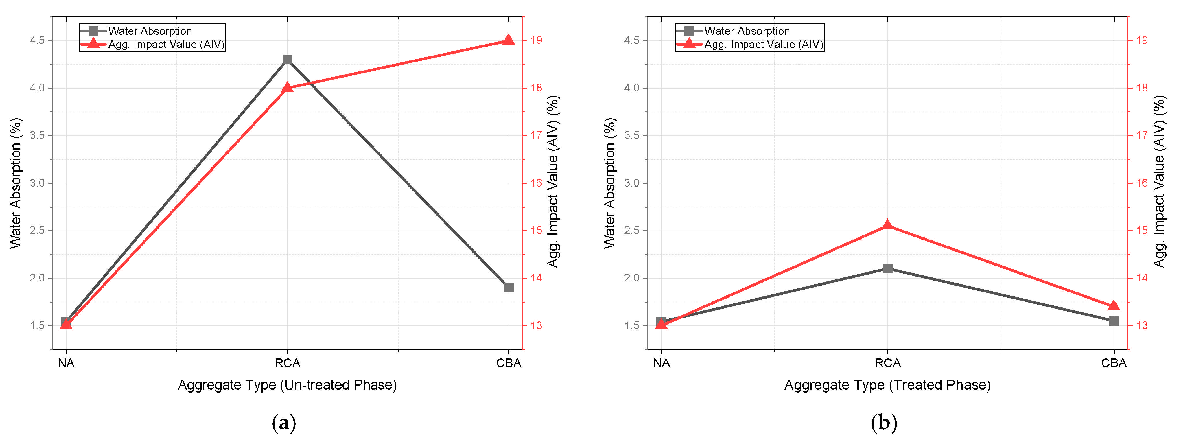
The laboratory results [7] demonstrated that the proposed geopolymer surface treatment significantly improved the physical characteristics of both recycled concrete aggregate (RCA), as shown in Figure 1a and Recycled Cement Block Aggregate (CBA), as shown in Figure 1b.

Before treatment, both recycled aggregates exhibited inferior properties compared to natural aggregate (NA), with untreated RCA showing the poorest performance, including a high-water absorption of 4.3% and an aggregate impact value (AIV) of 18%. However, after treatment with the alkaline-activated NaOH solution mixed with limestone powder and silica fume, the treated RCA showed a 36% reduction in water absorption (from 4.3% to 2.1%) and a 16% improvement in AIV (from 18% to 15.1%). Even more remarkably, the treated CBA achieved a water absorption of 1.55% and AIV of 13.4%, values almost identical to those of natural aggregate (1.5% water absorption and 13% AIV). These improvements were attributed to the filling and sealing effect of the geopolymer matrix, which effectively filled the surface voids and pores of the aggregates.

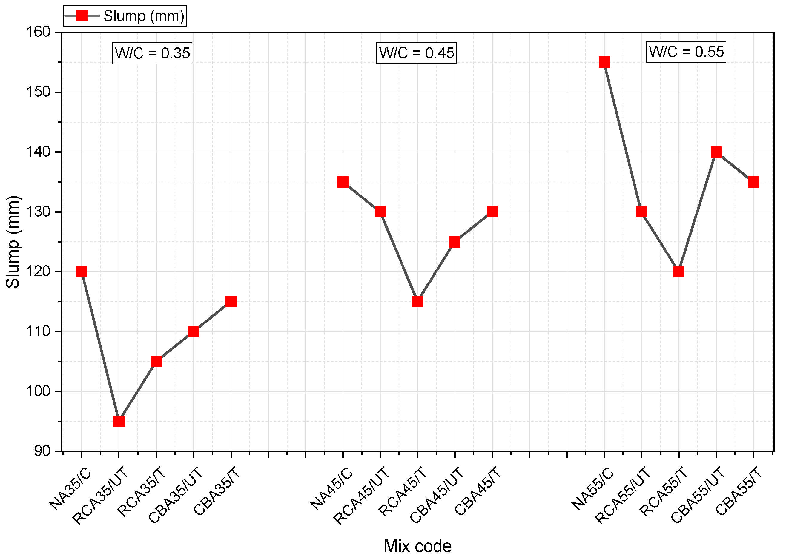
Also, while concrete mixes made with treated RCA only demonstrated improvements in slump at a 0.35 W/C ratio, concrete mixes made with treated CBA demonstrated improved slump values at both 0.35 and 0.45 W/C ratios, as shown in Figure 2. This is explained by the surface treatment’s filling-sealing effect, which fills all of the aggregate’s pores and voids and limits the amount of effective mixing water absorbed by the CBA or RCA during mixing, improving consistency. Notably, in terms of uniformity, concrete mixes made with treated or untreated CBA outperformed those made with treated or untreated RCA. This is explained by the fact that CBA absorbs less water than RCA, which improves uniformity. This is also consistent with research by Abd Al Kader A. Al Sayed et al. [7], who found that soaking in a cement–pozzolan solution increased the slump value of concrete made with treated RA.

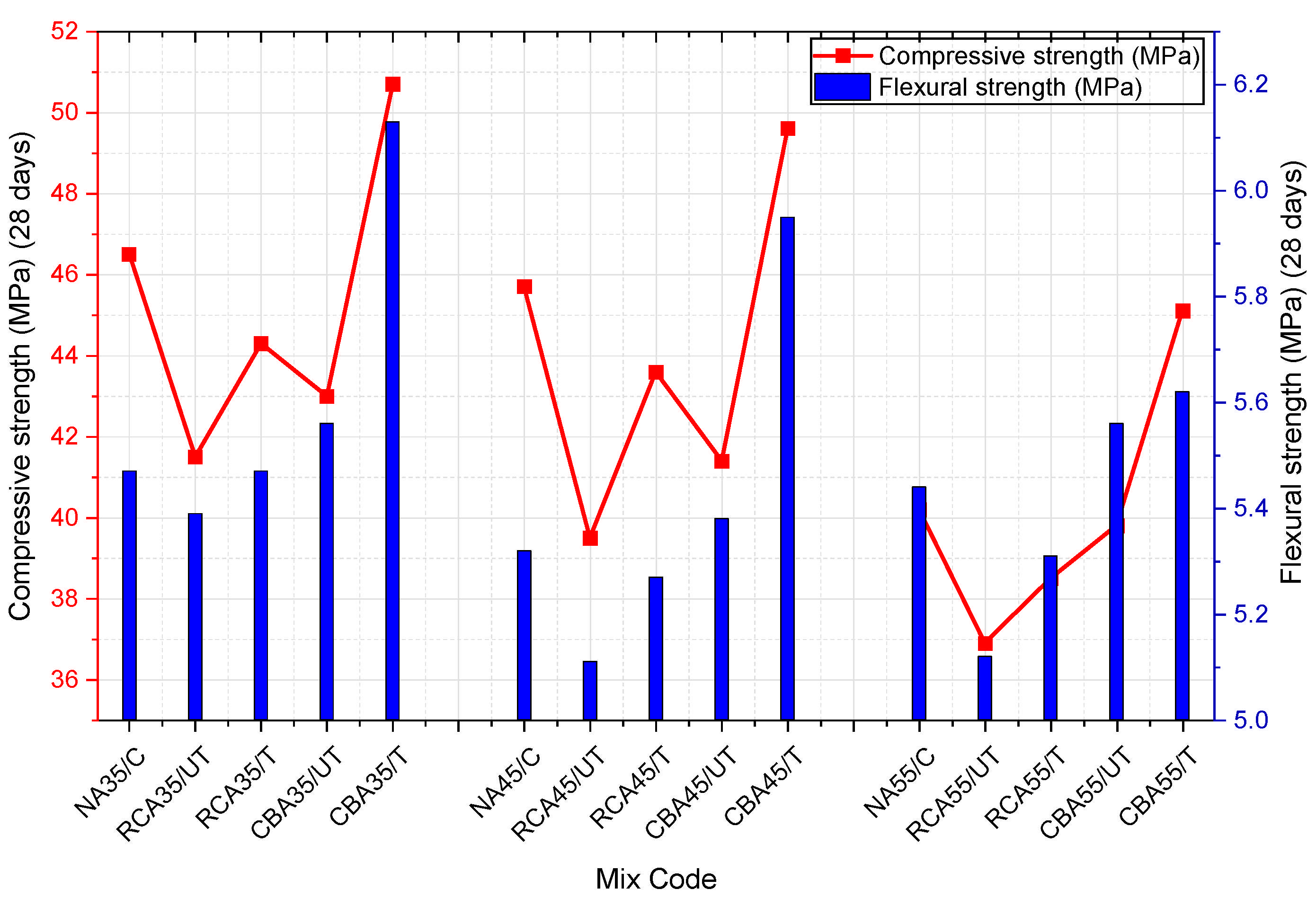
The compressive strength results revealed that the geopolymer treatment was highly effective, particularly for CBA-based concrete. At a water-to-cement ratio of 0.35, concrete produced with treated CBA achieved a 28-day compressive strength of 50.7 MPa, which was not only higher than untreated CBA (41.4 MPa) but also significantly exceeded the natural aggregate control mix (46.5 MPa), as shown in Figure 3. Similarly, treated RCA reached 44.3 MPa compared to 41.5 MPa for untreated RCA. The best performance was consistently recorded for treated CBA at the lowest W/C ratio of 0.35, producing a 28-day compressive strength increase of approximately 22.5% relative to its untreated counterpart. Regarding flexural strength, the treated CBA mix at W/C = 0.35 achieved the highest value of 6.13 MPa at 28 days, which was 10.5% higher than the control natural aggregate concrete (5.47 MPa) and 28% higher than untreated CBA concrete (5.56 MPa).

The treated RCA also showed modest improvements, with flexural strength increasing from 5.39 MPa (untreated) to 5.47 MPa (treated). The superior performance of treated CBA was attributed to the geopolymer matrix that provided strong interfacial bonding, enhanced particle interlocking, and reduced porosity, thereby improving load transfer and crack resistance.

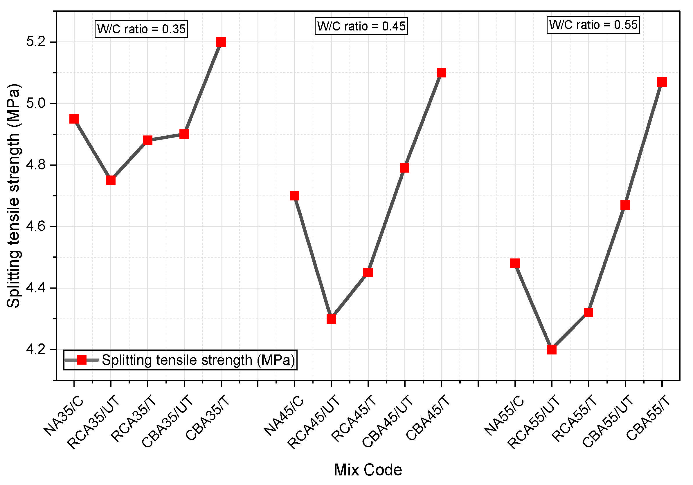
As shown in Figure 4, the splitting tensile strength tests followed a similar trend, confirming the effectiveness of the geopolymer treatment. At W/C = 0.35, the treated CBA concrete mix achieved the highest tensile splitting strength of 5.6 MPa at 28 days, exceeding both the natural aggregate control (4.9 MPa) and untreated CBA (4.9 MPa), representing a 14.3% improvement over the control. Treated RCA showed a more modest enhancement, from 4.75 MPa (untreated) to 4.88 MPa (treated), equivalent to a 2.76% increase. At higher W/C ratios of 0.45 and 0.55, treated CBA continued to outperform all other mixes, with tensile strength values of 5.1 MPa and 5.07 MPa, respectively, while treated RCA achieved 4.45 MPa and 4.32 MPa. Regarding water absorption, which is critical for durability, the treated CBA mixes showed the most substantial improvements. At W/C = 0.35, the water absorption of treated CBA concrete was reduced to 0.74% compared to 1.1% for untreated CBA, while treated RCA decreased from 0.96% to 0.88%. At W/C = 0.55, treated CBA achieved 1.2% water absorption versus 1.45% for untreated CBA. These reductions confirm that the geopolymer treatment effectively sealed the aggregate surface, limiting water ingress and enhancing the concrete’s durability.

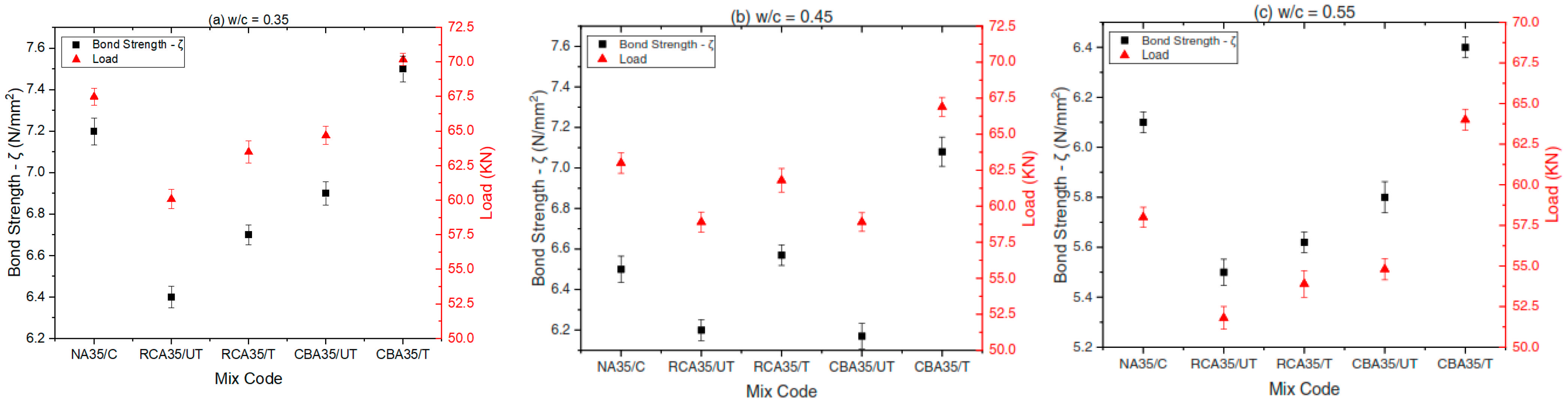
The pull-out test results provided critical evidence regarding the enhanced interfacial bonding between the steel reinforcement and recycled aggregate concrete. At the lowest W/C ratio of 0.35, the treated CBA concrete mix recorded the highest bond strength of 7.45 N/mm², which was superior to the natural aggregate control mix (7.17 N/mm²) and significantly higher than untreated CBA (6.87 N/mm²) and untreated RCA (6.38 N/mm²). Treated RCA achieved a bond strength of 6.74 N/mm² at the same W/C ratio, representing an improvement of approximately 5.6% over untreated RCA, as shown in Figure 5a. Similar improvements were observed at W/C = 0.45 (Figure 5b) and 0.55 (Figure 5c), where treated CBA consistently achieved the highest bond strength values of 7.02 N/mm² and 6.44 N/mm², respectively, while treated RCA reached 6.57 N/mm² and 5.62 N/mm². The enhanced bond strength was directly attributed to the geopolymer treatment, which improved the interfacial transition zone (ITZ) by filling voids and sealing micro-cracks on the aggregate surface. This resulted in superior mechanical interlocking and chemical adhesion between the geopolymer-treated aggregates and the surrounding cementitious matrix, ultimately improving load transfer and reducing the risk of rebar slip under stress.

It is important to emphasize that the pull-out bond strength predictions are valid only for the specific test geometry used in this study: 12 mm in diameter deformed steel bar, 100 mm bond length, and 150 mm in diameter × 300 mm in height concrete cylinders tested in accordance with ASTM C900-19 [47]. Bond strength is known to depend on numerous factors beyond aggregate type and W/C ratio, including rebar diameter, embedment length, concrete cover thickness, confinement conditions, rib geometry, casting position, and failure mode (pull-out vs. splitting).

The best overall performance was achieved by concrete produced with 100% treated cement block aggregate (CBA) at a water-to-cement ratio of 0.35. This optimal mix recorded a 28-day compressive strength of 50.7 MPa, a flexural strength of 6.13 MPa, a splitting tensile strength of 5.6 MPa, a bond strength of 7.45 N/mm², and a water absorption of only 0.74%. These values were not only superior to untreated CBA and untreated RCA mixes but also consistently exceeded the natural aggregate control mix across almost all mechanical properties. The treated CBA concrete demonstrated that it is fully suitable for structural applications, achieving a compressive strength of up to 51 MPa, which qualifies it for high-grade civil engineering uses. In comparison, the treated RCA mix at the same W/C ratio achieved a compressive strength of 44.3 MPa, which, while lower than treated CBA, still represents a substantial improvement over untreated RCA. The superior performance of treated CBA was attributed to its initially better physical properties compared to RCA, combined with the effective filling and sealing action of the geopolymer solution. The study conclusively demonstrated that the proposed innovative geopolymer surface treatment using alkaline-activated NaOH with limestone powder and silica fume is a powerful, cost-effective, and environmentally friendly method to enhance recycled aggregates. This technique can significantly promote the use of construction and demolition waste in the construction industry, reduce the depletion of natural resources, and support sustainable development goals. Notice that all the physical limitations were already addressed in the authors’ first research [7], which used the values and results of its practical program.

4. Dataset and Modeling

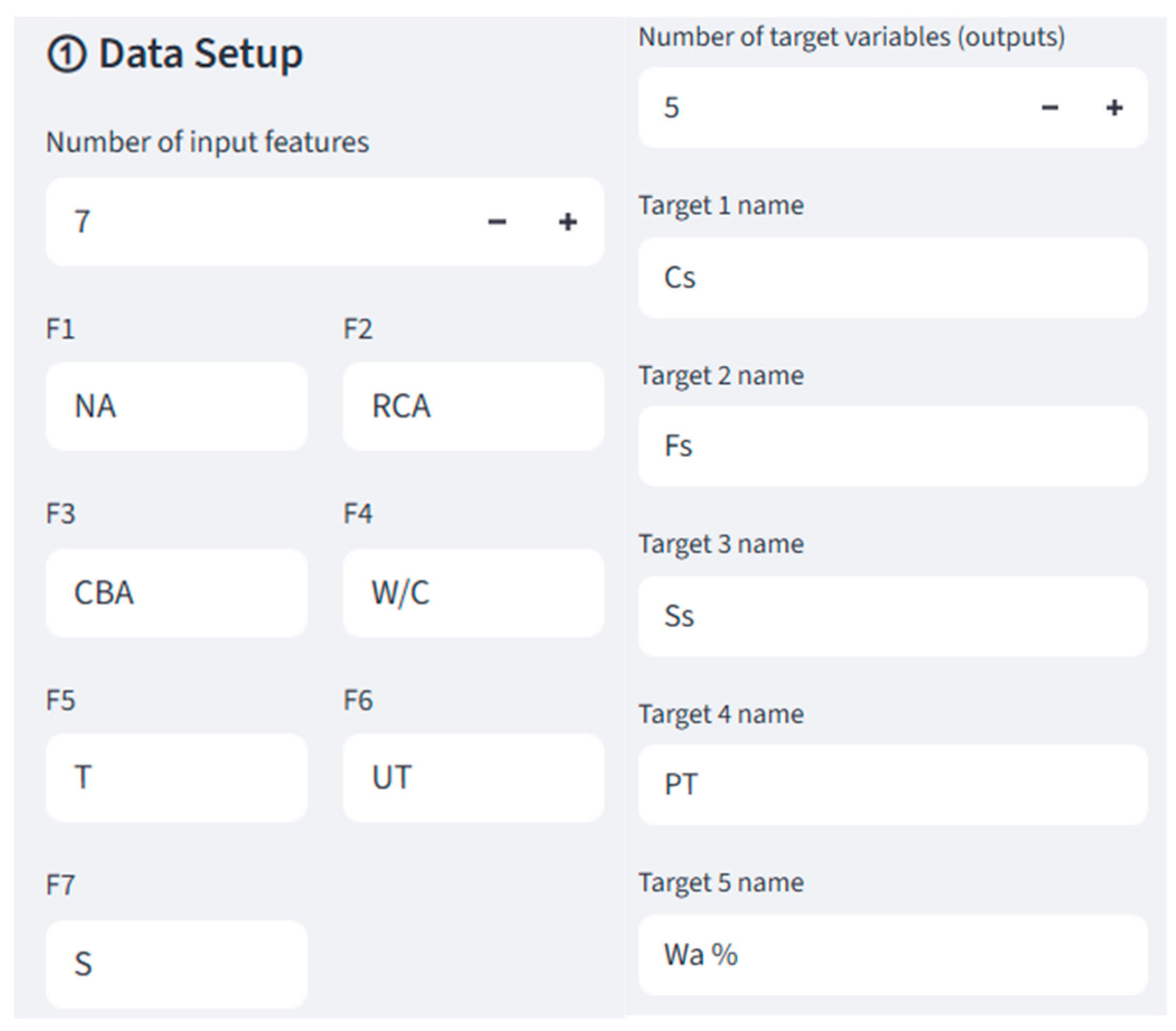
The linear regression (LR), M5P, Random Forest (RF), KNN and XGBoost models were developed and validated using a dataset of 360 data samples that was gathered from Abd Al-Kader A. Al Sayed in Ref. [7]. The data points of 360 tested specimens related to the compressive strength, splitting tensile strength, flexural strength, pull-out test and water absorption percentage findings for concrete combining different types of coarse aggregate (alkaline-treated or untreated) with other contents of mixture materials served as the foundation for the ML prediction models created in this study. As illustrated in Figure 6, concrete compressive strength (CS), splitting tensile strength (Ss), flexural strength (Fs), pull-out test (PT) and water absorption percentage (Wa%) were the responses, and the input variables were natural aggregate (NA), recycled concrete aggregate (RCA) and cement blocks aggregate (CBA) as the types of coarse aggregate, water-to-cement ratio (W/C), surface alkaline treatment case (treatment phase (T) and treatment phase (Un)) and the obtained slump (S). It should be noted that slump (S) is a measured property obtained from fresh concrete testing rather than a true mix design variable. Consequently, the models developed in this study are intended as post-test predictors that require slump as an input—meaning that they are suitable for the quality control and performance evaluation of already-batched concrete.

As part of the entire data preparation process, traditional machine learning starts with raw data and proceeds through feature extraction and data processing. Following an 80:20 ratio, the dataset was split into a train set for model development and a test set for model validation. A comprehensive assessment of the models’ prediction power under different circumstances was made possible by this division technique. The resulting model was calibrated and optimized using the training set. The models’ performance and generalizability on fresh data were evaluated using the other set. The dataset statistics are shown in

Table 2. Dataset statics.

Parameter	Min.	Max.	Mean	SD	Skewness	Kurtosis
NA	0	960	194.16	385.61	1.48	0.2
RCA	0	960	355.96	463.75	0.62	−1.62
CBA	0	960	355.96	463.75	0.62	−1.62
Water/Cement (W/C)	0.35	0.55	0.447	0.078	0.12	−1.23
Alkaline-Treated (T)	0	1	0.33	0.47	0.71	−1.5
Untreated (UT)	0	1	0.67	0.47	−0.71	−1.5
Slump (S)	91	155	123.4	15.2	0.35	−0.92
Compressive strength (Cs)	36.9	52.21	44.8	3.9	−0.21	−0.65
Flexural strength (Fs)	5.07	6.35	5.58	0.29	0.41	−0.43
Splitting tensile strength (Ss)	4.2	5.33	4.85	0.32	0.12	−0.98
Bond strength (PT)	5.5	7.64	6.55	0.59	−0.34	−0.72
Water absorption (Wa%)	0.64	1.59	1.02	0.28	0.55	−0.88

. Prior to model training, all five output variables (Cs, Fs, Ss, PT, Wa%) were normalized using z-score standardization (zero mean, unit variance) to ensure that variables with different units and scales received equal consideration during model optimization. With all other essential variables in the mixture remaining constant, such as cement, fine aggregate, and water content, the type of aggregate (NA, RCA or CBA) ranged from 0 to 960 kg, the W/C ratio ranged from 0.35 to 0.55, the surface alkaline treatment case ranged from 0 to 1 (0 means untreated and 1 means treated) and the slump (S) ranged from 91 to 155 mm. The output C_S ranged from 36.9 to 52.21 MPa, the output F_S ranged from 5.07 to 6.35 MPa, the output S_S ranged from 4.2 to 5.33 MPa, the output PT ranged from 5.5 to 7.64 MPa and the output Wa% ranged from 0.64 to 1.59%. The skewness and kurtosis values were within the permissible ranges of (−3 to + 3) and (−10 to + 10), respectively.

All of the variables’ skewness values fell between −3 and +3, suggesting a reasonable degree of distributional symmetry. The current study met the appropriate range of kurtosis, which is −10 to +10, suggesting a sufficient degree of peaks and distribution in the model variables [19,25,38,48].

The optimal hyperparameters were selected based on the lowest validation RMSE and were then used to retrain the final models on the full training set. This procedure ensures that hyperparameters are tuned without any information leakage from the test set.

4.1. Correlation Coefficient (R)

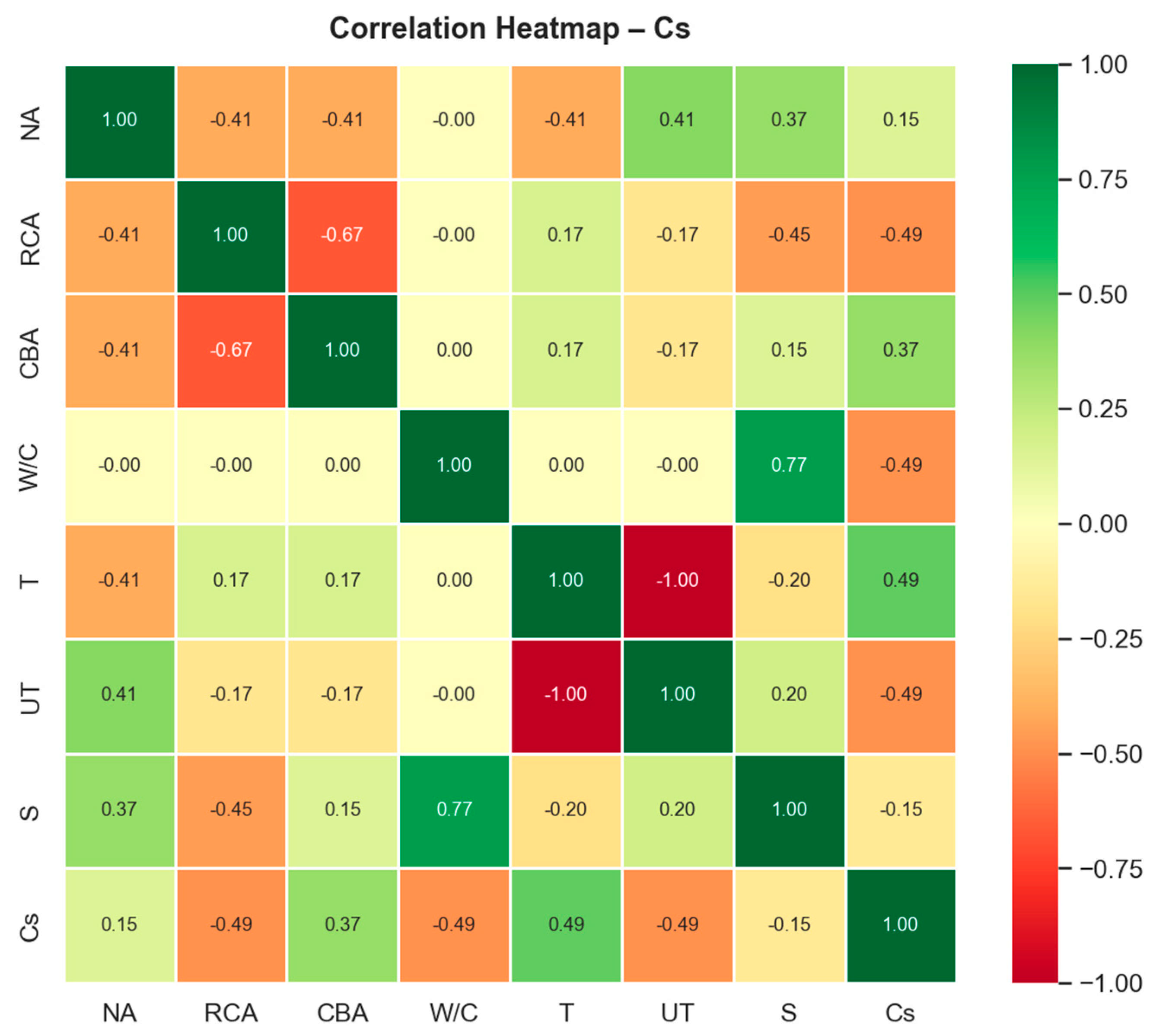
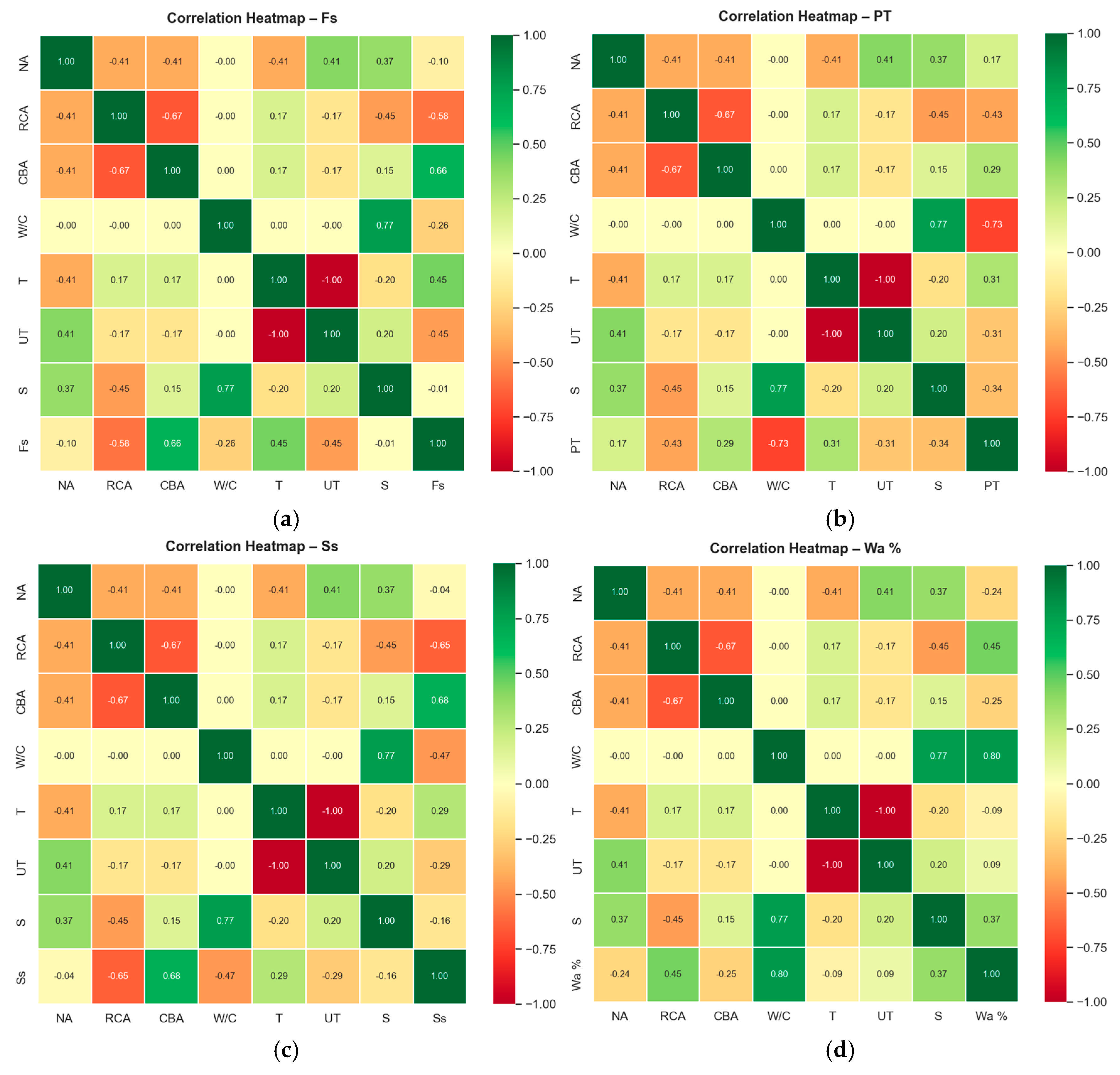
Pearson’s correlation coefficient (R) was employed to evaluate the relationships between the output variables (Cs, Fs, Ss, PT, and Wa%) and the input parameters (NA, RCA, CBA, W/C, T, UT, and S). Separate heatmaps were generated for each output, while only the compressive strength (Cs) heatmap is presented in Figure 7 to illustrate the interactions between input variables and Cs. The results indicate that Cs exhibits weak-to-moderate linear correlations with most inputs, including weak positive correlations with NA (0.15) and CBA (0.37), a weak negative correlation with slump (−0.15), moderate negative correlations with RCA and W/C (both −0.49), and moderate positive and negative correlations with treated (T, 0.49) and untreated aggregates (UT, −0.49), respectively.

Also, the Pearson correlation matrices serve as a linear screening tool to identify potential relationships between inputs and outputs. It is important to emphasize that a zero or near-zero Pearson correlation does not imply the absence of a relationship; rather, it indicates the absence of a linear relationship. Nonlinear relationships such as threshold effects, saturation, or interactions are invisible to Pearson correlation and may still be captured by nonlinear AI models.

Notably, T and UT show a perfect negative correlation of −1.00, indicating strict mathematical redundancy (one is likely the inverse or complement of the other), and W/C and S also display a strong correlation of 0.77, both of which pose multicollinearity issues, especially for statistical models. The lack of strong linear correlations (|r| > 0.7) with compressive strength (Cs) indicates that AARAC behavior is governed by complex nonlinear interactions among mix parameters. Therefore, conventional regression models may underperform, whereas AI techniques such as ANN, RF, and XGBoost are better suited to capture hidden patterns and interaction effects. To improve model reliability, removing redundant variables such as T or UT and addressing multicollinearity between W/C and slump is recommended. Correlation analysis further revealed that the water-to-cement ratio (W/C) strongly influences concrete performance.

It exhibited a strong positive correlation with water absorption (Wa%, r ≈ 0.80) and negative correlations with pull-out strength (PT, r ≈ −0.73), splitting tensile strength (Ss, r ≈ −0.47), and flexural strength (Fs), confirming the adverse effects of excessive water content on strength and durability. Aggregate type also significantly affected performance. RCA showed negative correlations with mechanical properties and a positive correlation with Wa%, reflecting its porous nature. In contrast, CBA exhibited positive relationships with strength properties and lower permeability, suggesting beneficial filler and pozzolanic effects under alkali activation. Aggregate treatment improved concrete behavior, with treated aggregates (T) being positively correlated with Fs, Ss, and PT and negatively correlated with Wa%, demonstrating the effectiveness of alkali-activated surface treatment. Conversely, untreated aggregates (UT) showed the opposite trend. Slump was positively correlated with W/C but weakly or negatively related to mechanical properties, indicating that excessive workability may reduce concrete strength.

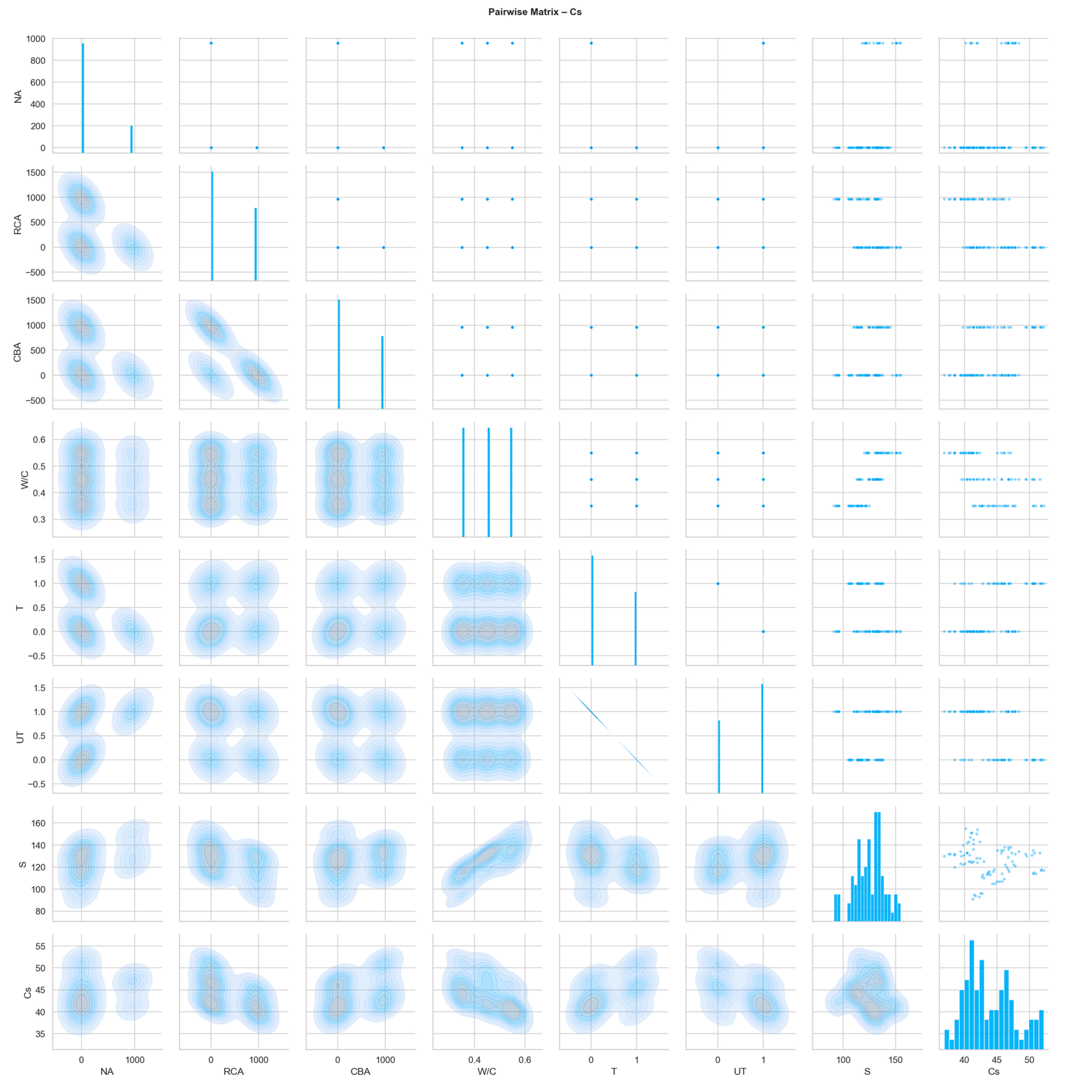
Also, Figure 8 presents the pairwise correlation matrix illustrating the relationships between the input variables, namely natural aggregate (NA), recycled concrete aggregate (RCA), Crushed Brick Aggregate (CBA), water-to-cement ratio (W/C), treated aggregate condition (T), untreated aggregate condition (UT), and slump (S), with the output parameter represented by compressive strength (Cs). The pairwise visualization provides important insights into the interaction behavior among variables and their influence on the prediction capability of the developed AI and statistical models.

The matrix indicates that the compressive strength (Cs) is significantly influenced by the aggregate composition and treatment conditions. A noticeable positive correlation is observed between Cs and the treated recycled aggregate parameter (T), suggesting that alkali-activated surface treatment contributed effectively to improving the mechanical performance of recycled aggregate concrete. This enhancement can be attributed to the improvement in the interfacial transition zone (ITZ) and the reduction in aggregate porosity after treatment. In contrast, the untreated aggregate condition (UT) demonstrates a comparatively weaker or slightly negative relationship with compressive strength, indicating the adverse effect of untreated recycled aggregates on concrete performance due to higher water absorption and weaker bonding characteristics.

The pairwise plots also reveal that the water-to-cement ratio (W/C) exhibits an inverse relationship with Cs, where increasing W/C generally results in lower compressive strength values. This trend agrees with conventional concrete behavior, as higher water content increases pore volume and weakens the hardened matrix structure. Additionally, slump (S) shows a moderate correlation with Cs, indicating that workability variations may indirectly affect the density and compaction quality of the concrete mixtures. Regarding aggregate types, the relationships between NA, RCA, and CBA demonstrate complex interaction patterns.

The increase in recycled aggregate content, particularly RCA and CBA, tends to slightly reduce compressive strength due to the weaker nature of recycled particles compared with natural aggregates. However, the presence of treated recycled aggregates mitigates this reduction and improves the overall mechanical behavior. The density contours observed in the pairwise distributions indicate clustered regions corresponding to specific mixture combinations, reflecting the consistency and reliability of the experimental dataset used for AI model training.

Furthermore, the diagonal distributions and scatter-density plots suggest that the dataset possesses sufficient variability and balanced parameter ranges, which enhances the robustness of machine learning models, including XGBoost, Random Forest (RF), K-Nearest Neighbors (KNN), and M5P. The observed nonlinear and multidirectional relationships between several variables and Cs confirm the necessity of employing advanced AI-based prediction techniques rather than relying solely on traditional linear statistical methods. Overall, the pairwise correlation analysis demonstrates that the aggregate treatment condition, W/C ratio, and recycled aggregate type are among the most influential parameters governing the compressive strength behavior of alkali-activated recycled aggregate concrete.

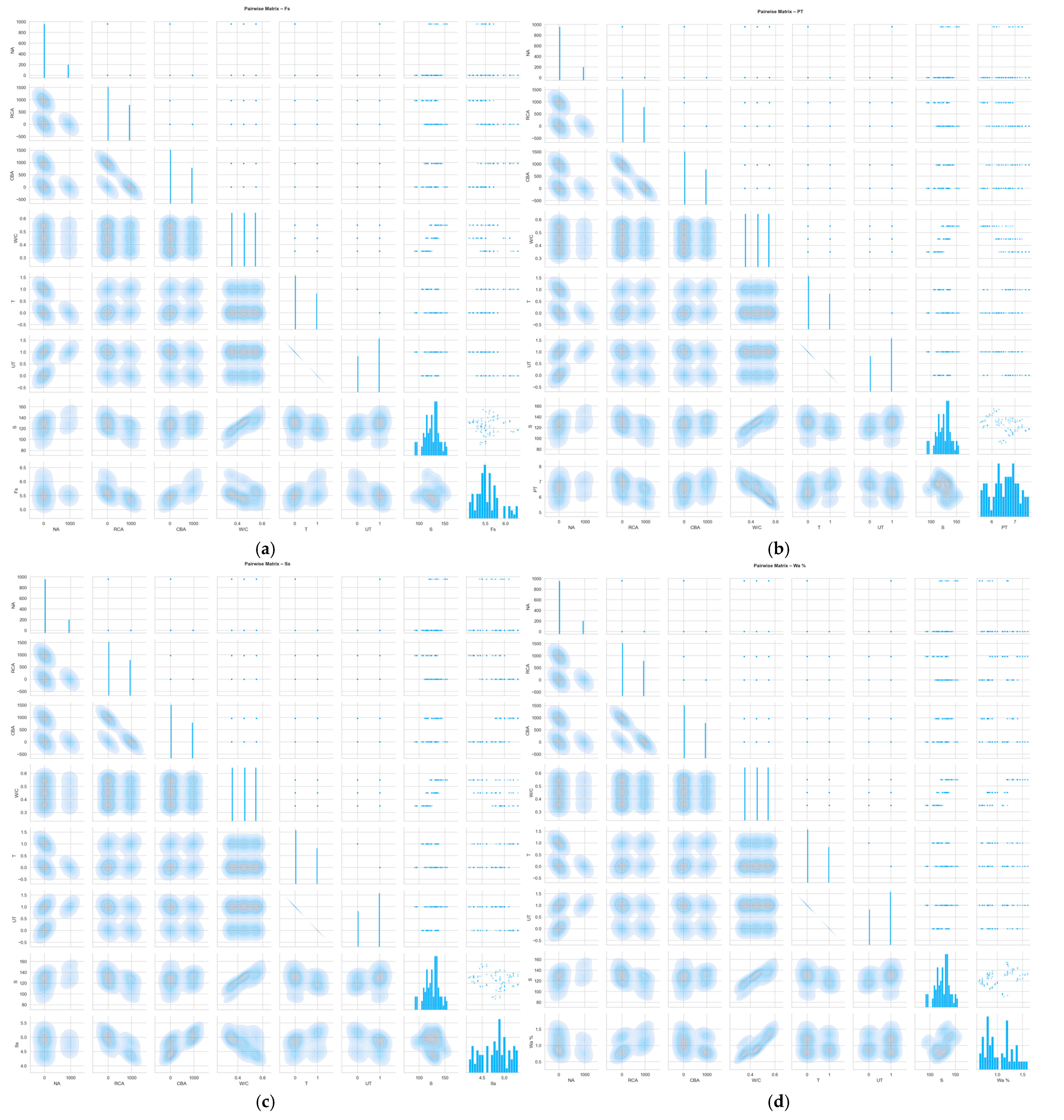
Similarly, according to Appendix A—Figure A2, and in the same context, after studying the other four outputs “Fs, Ss, PT, and Wa%”, the pairwise correlation matrices reveal that linear relationships between the input variables (NA, RCA, CBA, W/C, T, UT, S) and the mechanical outputs are generally weak or absent. For Fs and Wa%, the matrices consist almost entirely of zero entries, indicating a negligible Pearson correlation. The PT matrix contains only one moderate negative value (−0.502) for a single input–output pair, while all other PT correlations are zero. In contrast, the Ss matrix shows non-zero values (e.g., positive effects for NA, CBA, UT, and T, with relative scores up to 1.5), suggesting that splitting tensile strength exhibits some linear dependence on certain inputs. However, even for Ss, the presence of negative symbols and variability in the values points to nonlinear components, especially for RCA and W/C. Overall, the matrices confirm that most outputs do not vary linearly with mix proportions or curing conditions, and that threshold effects, interactions, and curvilinear trends dominate the behavior of alkali-activated recycled aggregate concrete.

Because the pairwise linear correlations are predominantly zero or very weak, conventional statistical models (e.g., multiple linear regression) would perform poorly in predicting Fs, PT, and Wa%, and only moderately for Ss. The near-absence of a linear structure indicates that the underlying relationships are nonlinear and often non-monotonic; for instance, pulse velocity depends on porosity thresholds, water absorption jumps sharply when recycled aggregate content exceeds ~40%, and flexural strength peaks at an optimal water-to-cement ratio before declining. In contrast, artificial intelligence models such as artificial neural networks, Random Forests, and support vector machines with nonlinear kernels are inherently capable of capturing such complex patterns. They learn threshold effects, interactions between inputs (e.g., temperature × ultrasound velocity), and saturation behaviors that are invisible to linear correlation analysis. Therefore, the pairwise matrix results strongly justify the use of advanced AI techniques over statistical regression for accurately predicting the mechanical properties of alkali-activated recycled aggregate concrete, as AI models can exploit the hidden nonlinear information that the pairwise matrices fail to reveal.

Multicollinearity Assessment

The Pearson correlation analysis revealed a perfect negative correlation (r = −1.00) between treated (T) and untreated (UT) variables, indicating complete redundancy. Variance Inflation Factor (VIF) analysis confirmed severe multicollinearity (VIF > 100). While this poses a significant issue for linear regression—leading to unstable coefficient estimates and reduced generalization (R² = 0.696)—ensemble tree models (RF, XGBoost, M5P) are inherently robust to multicollinearity due to their feature-splitting mechanism. To quantify the effect, we trained RF with and without UT; the test R² changed by only −0.0017 (from 0.8736 to 0.8719), confirming minimal impact. We recommend that practitioners remove one variable when using linear or logistic regression but retain both for tree-based models where interpretability is prioritized.

Also, to address the perfect multicollinearity between T and UT (r = −1.00), UT was removed from all model training as a predictor variable, and only T (treated = 1, untreated = 0) was retained as a binary predictor. This decision was made prior to any model training and applies consistently across all five models (LR, M5P, RF, KNN, XGBoost). Consequently, the final feature set used for all model development comprised six input variables: NA, RCA, CBA, W/C, T, and S. The UT variable appears in the linear regression equations (Equations (9)–(13)) and M5P leaf models (

Table 3. Results of the models’ performance metrics “According this type of data”.

	R2		MAE		RMSE		MAPE
	Train	Test	Train	Test	Train	Test	Train	Test
M5P	0.87539	0.759544	0.085277	0.104041	0.103829	0.129248	1.534436	1.875385
RF	0.974874	0.873645	0.03824	0.078271	0.046623	0.093692	0.69386	1.417948
XGBoost	0.981377	0.86054	0.031754	0.086032	0.040139	0.098431	0.576855	1.556974
KNN	0.905194	0.771671	0.07577	0.095556	0.090565	0.125947	1.363207	1.699376
LR	0.779816	0.69581	0.113642	0.117885	0.138018	0.145372	2.037709	2.147216

) solely for mathematical completeness to illustrate the perfect negative correlation, but it was excluded from all model training and prediction. Table 1 retains UT for descriptive completeness of the dataset only.

To quantify the impact of this removal, we trained the Random Forest model with and without UT; the test R² changed by only −0.0017 (from 0.8736 to 0.8719), confirming minimal impact on tree-based ensemble models. For linear regression, we performed a separate analysis: when both T and UT were included, the coefficients were unstable with inflated standard errors (VIF > 100), and the test R² dropped from 0.6958 to 0.6723 due to numerical instability. Therefore, UT was excluded from all final models, and all reported results reflect this corrected feature set. The dataset statistics table (Table 1) retains UT for descriptive completeness, but all modeling excludes it.

4.2. Methodology

Linear regression (LR) and three machine learning algorithms, the M5P model tree, the Random Forest (RF) algorithm, KNN and the XGBoost algorithm are the foundation of this study’s methodology. The models’ effectiveness was confirmed using statistical metrics like MAE, RMSE, R, and MAPE, and their accuracy was confirmed by external K-fold cross-validation. Statistical measures like MAE, RMSE, R, and MAPE were used to confirm the models’ effectiveness. To verify the models’ accuracy, external K-fold cross-validation was used for model validation.

4.2.1. Linear Regression (LR)

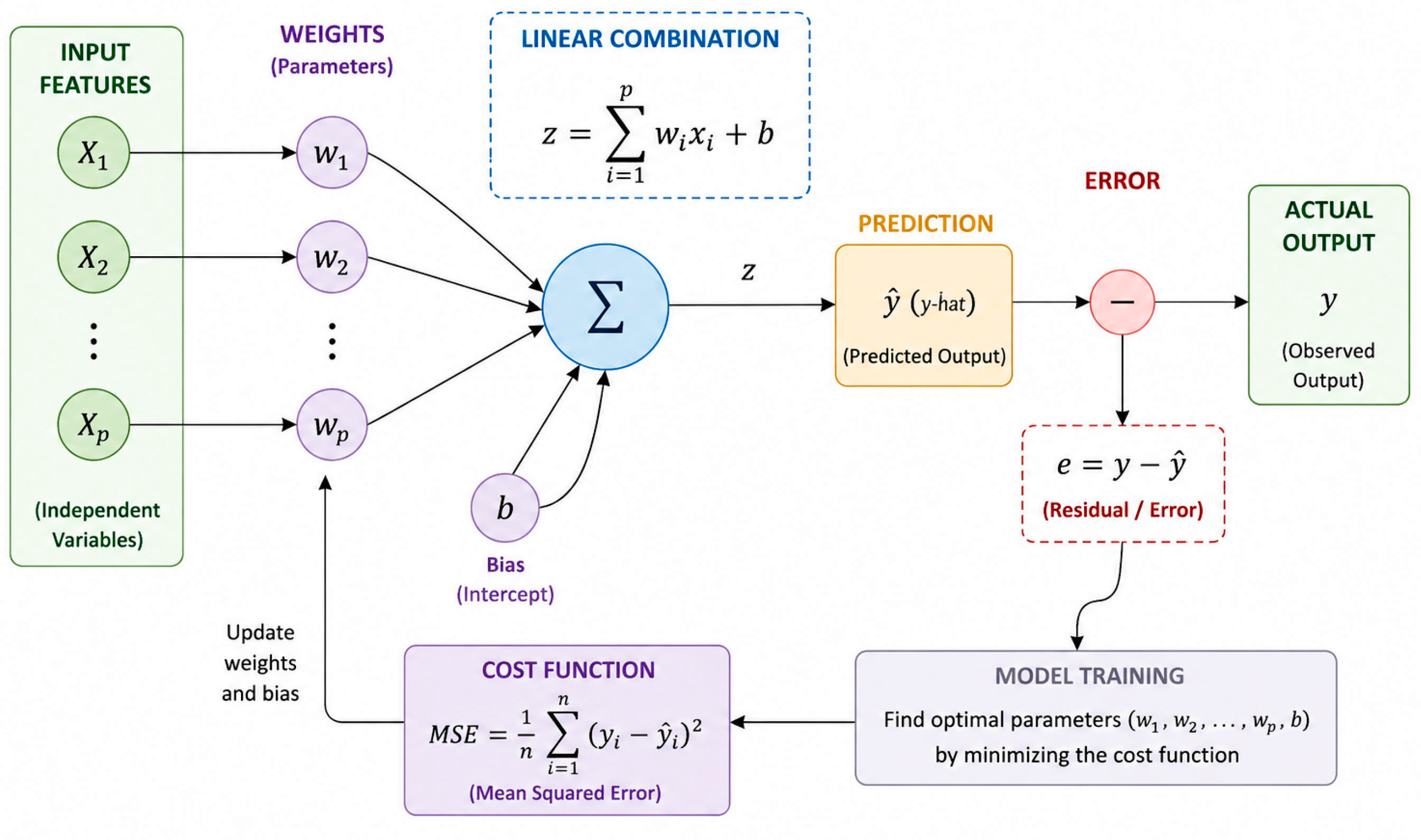
According to Figure 9, linear regression is a foundational statistical method that models the relationship between a dependent (target) variable and one or more independent (predictor) variables by fitting a linear equation to the observed data, as seen in Equation (1). Its primary goal is to find the best-fitting straight line through the data points. For multiple independent variables, the model is expressed as:

$$y=b_0+b_1{x}_1+b_2{x}_2+\dots +b_n{x}_n$$

(1)

where “$y$” is the predicted output; $x_1$, $x_2$, …, $x_n$ are the input parameters (e.g., NA, CBA, slump); $b_0$ is the intercept; and $b_1$, $b_2$, …, $b_n$ are the coefficients representing each input’s influence.

The model’s structure is represented by a straight line in a scatter plot, minimizing the sum of squared residuals. It relies on the input variables having a linear relationship with the output, with minimal multicollinearity. To predict a new concrete mix’s strength, the known mix parameters are entered into the equation, and the result is calculated. It is a simple and interpretable model but often struggles to capture the non-linear complexities of concrete’s mechanical behavior, as noted in the study. This model is particularly valuable as a baseline for comparison against more advanced, non-linear models.

4.2.2. M5P Model Tree

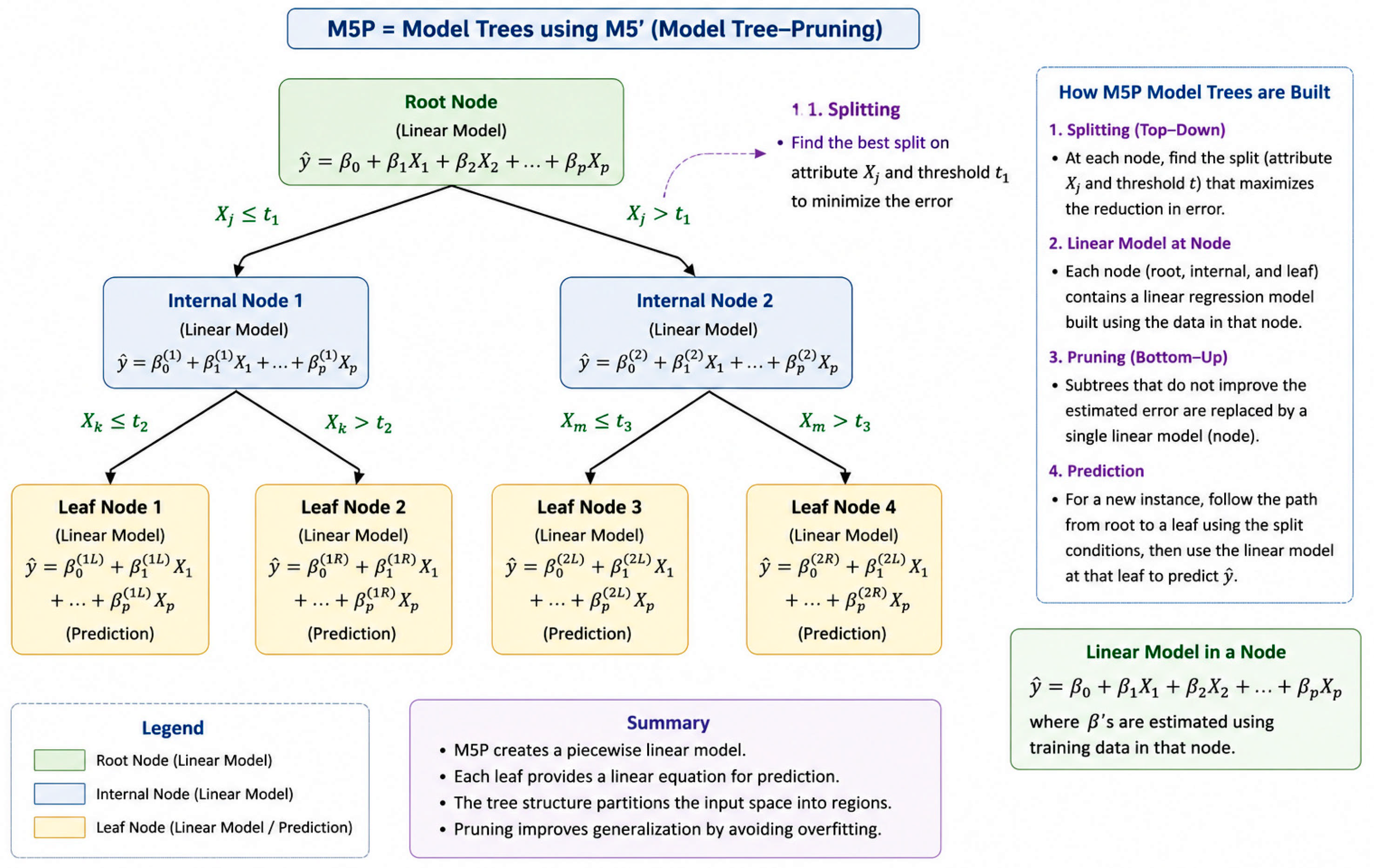
The M5P algorithm as shown in Figure 10, is a regression tree method that constructs a decision tree-like structure, but instead of constant values, its leaves contain linear regression equations. This hybrid approach makes it well-suited for datasets with non-linear characteristics, as it partitions the input space into smaller, more manageable regions where linear models apply effectively. The model’s general shape is shown in Equation (2), where a, b, c, d, and e are linear regression constants. For example,

CS = a (NA) + b (CBA) + c (RCA) + d(W/C) + e(T) + f(UT) + g(S)

(2)

The structure is a tree where internal nodes contain conditions (e.g., “if Cement < 400 kg/m³”) and concrete contains linear regression models. This creates “if-then” rules that are easy to interpret. For prediction, a new data point enters at the root and moves down based on conditions until it reaches a leaf, where the associated linear equation is used to compute the predicted strength. This model is more powerful than standard linear regression but remains more interpretable than “black box” models.

4.2.3. Random Forest (RF)

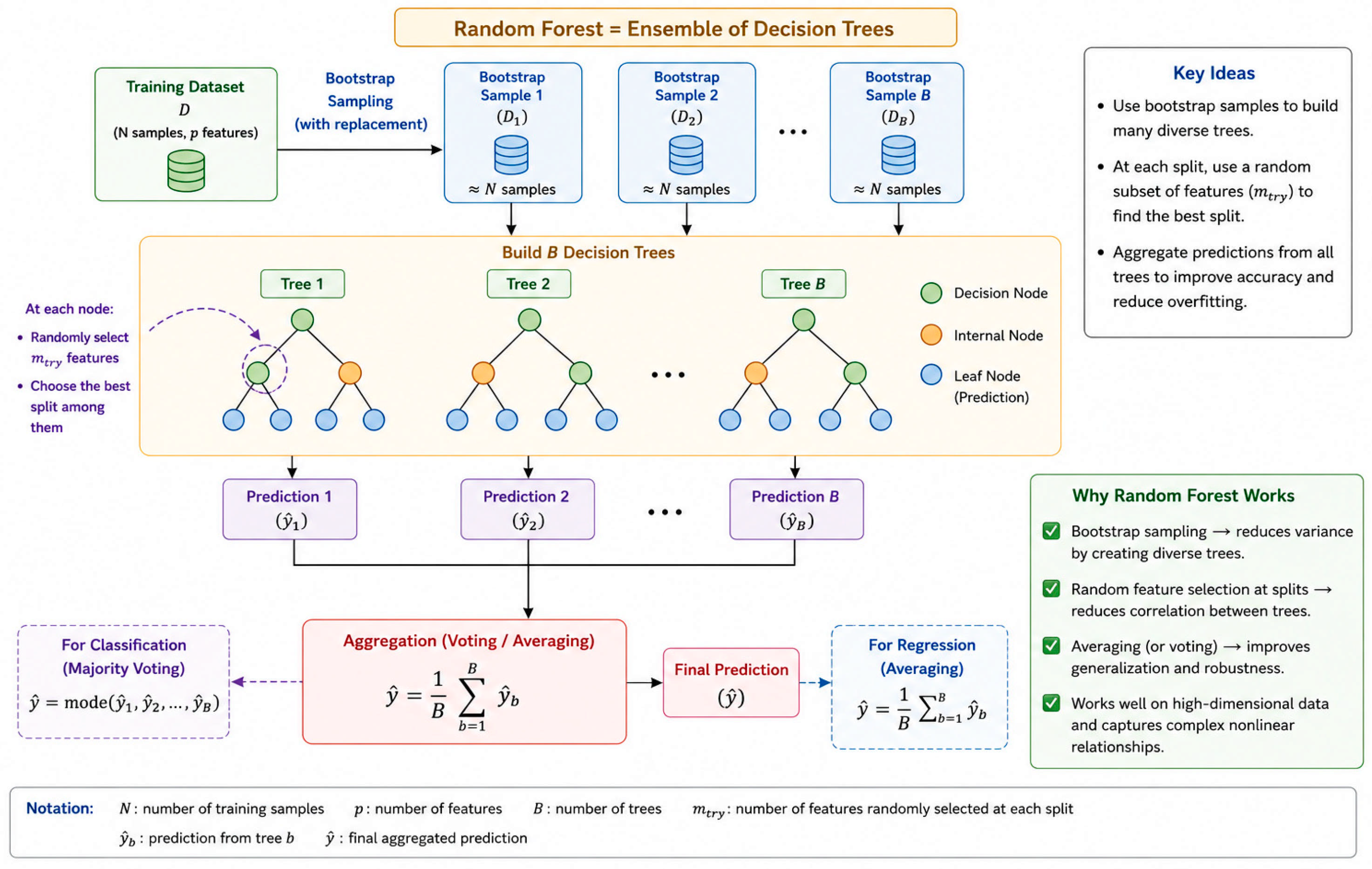
Random Forest as shown in Figure 11, is an ensemble learning method that constructs a multitude of decision trees at training time and outputs the average prediction of the individual trees. It is highly robust to overfitting and can model complex, non-linear interactions between variables without requiring extensive fine-tuning. The prediction $\widehat{y}$ is the average of all the individual decision tree predictions, as seen in Equation (3):

$$\widehat{y}={\displaystyle \frac{1}{B}}{\sum }_{b+1}^B{T}_b\left(x\right)$$

(3)

where “B” is the total number of trees in the forest and $T_b\left(x\right)$ is the prediction from the b-th tree. Random Forest combines predictions from multiple decision trees trained on random data and feature subsets. The final prediction is obtained by averaging individual tree outputs, improving accuracy and generalization. The model also identifies the relative importance of input variables in reducing prediction error.

4.2.4. K-Nearest Neighbors (KNN)

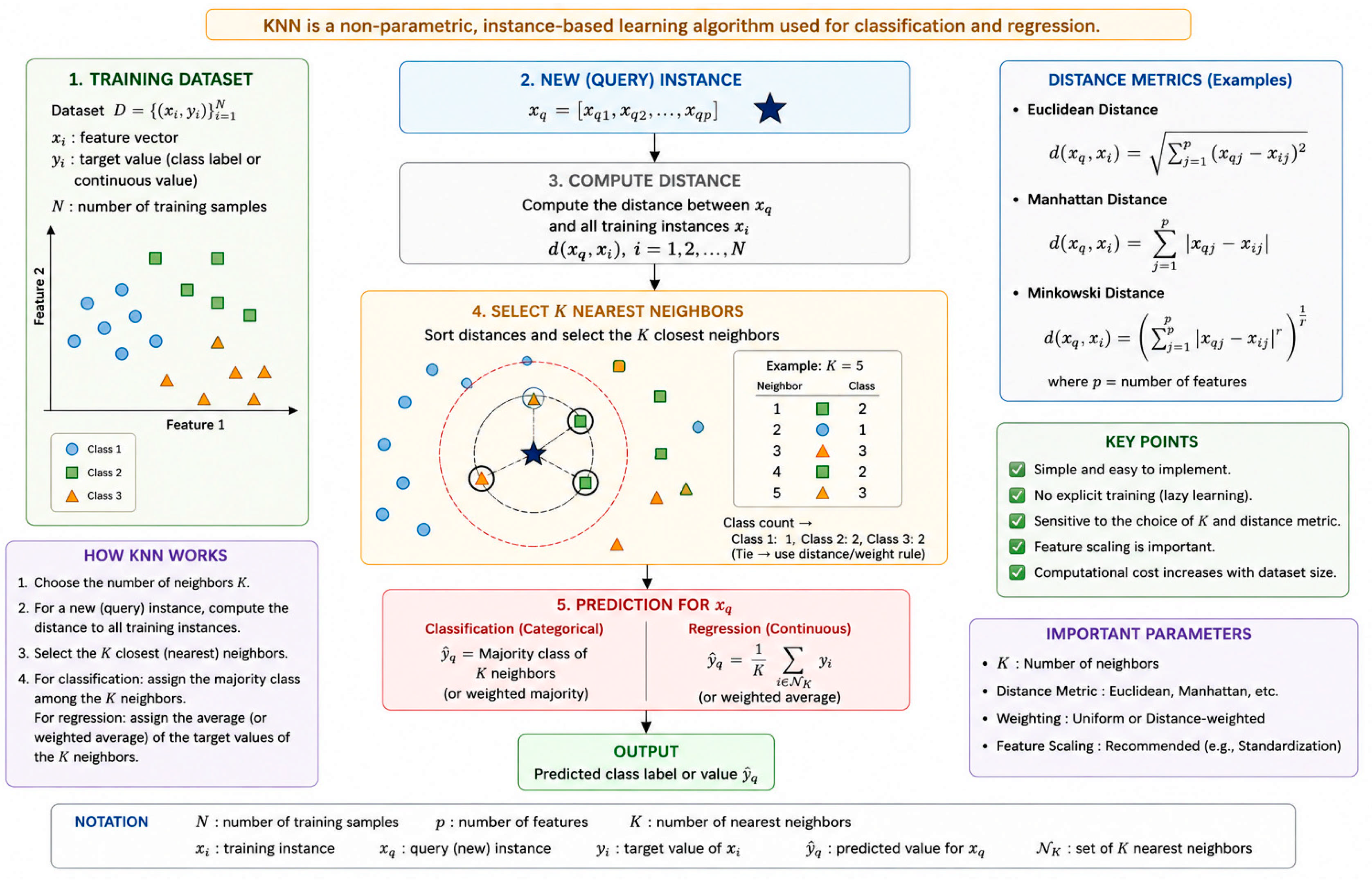
K-Nearest Neighbors is a non-parametric, instance-based learning algorithm. It is considered a “lazy learner” because it does not explicitly learn a model from the training data. Instead, it memorizes the training dataset and makes predictions for a new data point by identifying the “$k$” most similar examples (neighbors) from the training data. The prediction $\widehat{y}$ is the average of the target values $y_i$ of the “$k$” Nearest Neighbors to the new point x, as seen in Equation (4):

$$\widehat{y}={\displaystyle \frac{1}{k}}{\sum }_{i=1}^k{y}_i$$

(4)

where neighbors are determined by a proximity measure, typically Euclidean distance.

As shown in Figure 12, the model’s structure is essentially the entire training dataset visualized in a multi-dimensional space. The algorithm relies on three key elements: a distance metric (e.g., Euclidean), a value for “k”, and a decision rule (averaging for regression). When a new concrete mix is to be predicted, the algorithm calculates its distance from all mixes in the training data. It then finds the k closest ones and averages their experimentally measured strengths to produce the prediction. The KNN model has been successfully applied in various concrete research studies for its simplicity and effectiveness, particularly when combined with optimization techniques.

4.2.5. XGBoost (Extreme Gradient Boosting)

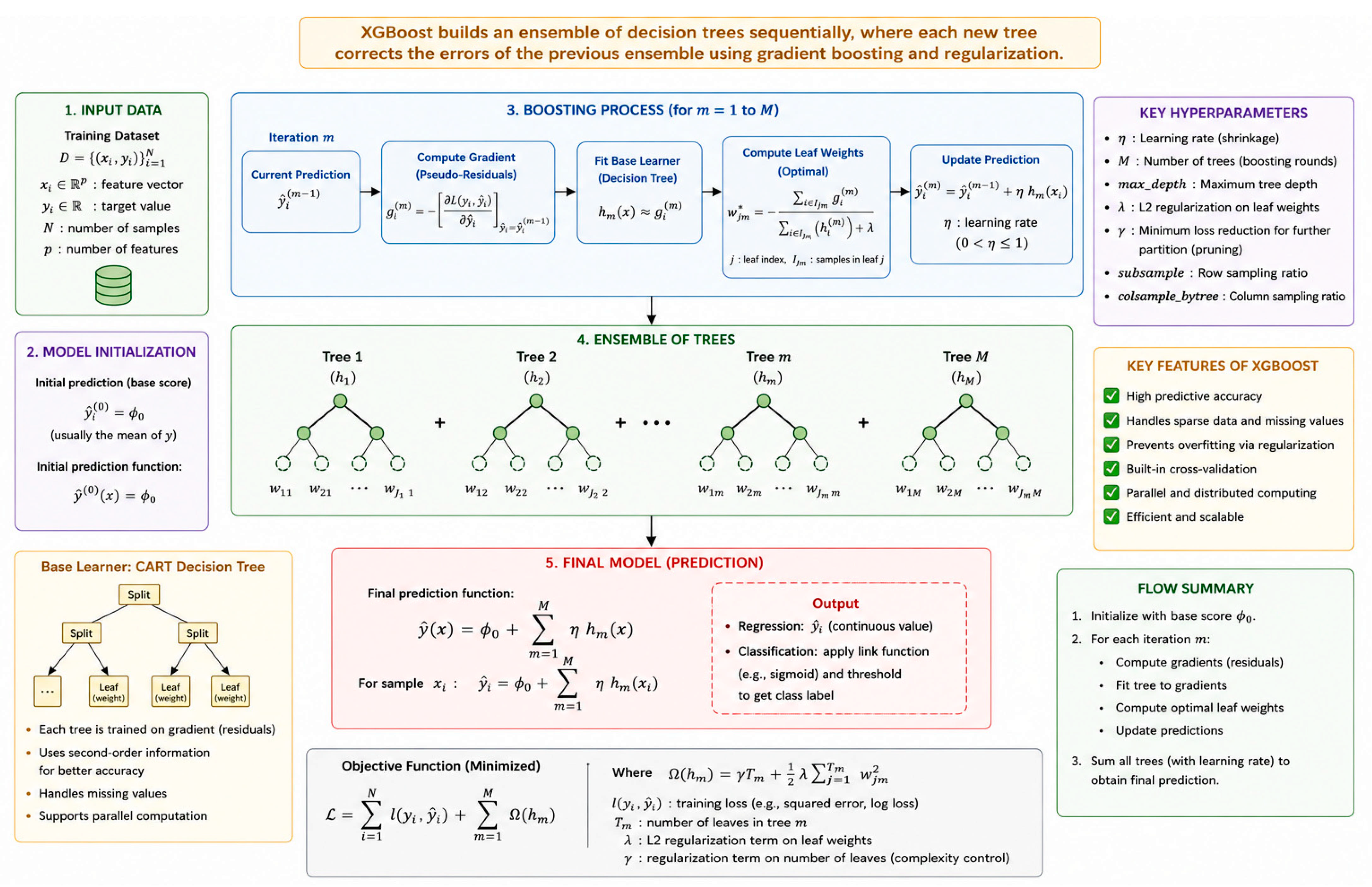
XGBoost enhances prediction accuracy by combining multiple decision trees in a gradient-boosting framework, where each new tree learns from the errors of previous ones. This sequential learning process improves model performance, making XGBoost highly effective for both classification and regression tasks.

As shown in Figure 13, the XGB algorithm, which combines the benefits of several machine learning techniques, including gradient boosting and decision trees, is used to create a predictive model with high accuracy and generalizability. Decision trees and other weak learners are used to iteratively improve the ensemble by adding new trees that address the errors made by the previous ones. Compared to alternative techniques, it shows enhanced capability in handling multiple features, operates efficiently with high-dimensional data, reduces overfitting through the inclusion of a regularization term, and improves the loss function via the second-order Taylor series expansion.

4.2.6. Model Efficiencies

The built models evaluated a number of performance statistical metrics, such as root mean square error (RMSE), mean absolute percentage error (MAPE), mean absolute error (MAE), and R². RMSE is a commonly used metric for evaluating the accuracy of predictive models. It measures the difference between expected and actual values; a lower RMSE indicates a superior model fit to the data, as we aim for minimal discrepancies between projections and actual outcomes. A measure of the discrepancy between experimental and expected measurements is called MAE. One of the most popular metrics for estimating error in statistical and machine learning models is mean absolute error (MAE). The mathematical expression for MAE is shown in Equation (5). RMSE is a commonly used statistic for evaluating predictive model accuracy. The difference between expected and actual values is measured by RMSE. As we strive for small differences between predictions and actual results, a lower RMSE denotes a better model fit to the data. Equation (6) provides an example of the mathematical expression for RMSE. A popular statistic for evaluating model prediction accuracy is called MAPE. As shown in Equation (7), it calculates the average absolute percentage errors of the actual and anticipated values. Reduced MAPE, MAE, and RMSE values show improved model performance, with predictions that closely resemble real values. A higher R2 suggests that a significant portion of the variance in the independent variable is explained by the dependent variable. The expression for R2, which ranges from 0 to 1 and serves as a gauge of the effectiveness of model fit, is shown in Equation (8).

$$MAE={\displaystyle \frac{1}{m}}{\sum }_{i=1}^m\left|(X_i-y_i)\right|$$

(5)

$$RMSE=\sqrt{{\displaystyle \frac{{\sum }_{i=1}^m{(X_i-y_i)}^2}{n}}}$$

(6)

$$MAPE={\displaystyle \frac{1}{m}}{\sum }_{i=1}^m{\displaystyle \frac{(X_i-y_i)}{X_i}}$$

(7)

$$R^2=\left[{\displaystyle \frac{{\sum }_{i=1}^m(x_i-\widehat{x})(y_i-\widehat{y})}{{\sum }_{i=1}^m{(x_i-\widehat{x})}^2{(y_i-\widehat{y})}^2}}\right]$$

(8)

where $x_i$ and $y_i$ are the actual and predicted values of Cs, Fs, Ss, PT, and Wa%; y is the means of experimental and predicted, respectively; and m is the number of data points.

4.2.7. Hyperparameter Optimization

Hyperparameter optimization was performed using Optuna, an automated hyperparameter optimization framework that employs Bayesian optimization with Tree-structured Parzen Estimators (TPE). The search process was designed to minimize overfitting while maximizing test performance. For each model, hyperparameters were tuned using 5-fold cross-validation on the training set (80% of data), with the validation RMSE used as the objective function.

For Random Forest, the search ranges were n_estimators (50–300), max_depth (5–20), min_samples_split (2–10), min_samples_leaf (1–5), and max_features (“sqrt”, ”log2”, None). The optimal values identified were n_estimators = 100, max_depth = 10, min_samples_split = 5, min_samples_leaf = 2, and max. features = “sqrt”. These conservative settings (moderate tree depth, relatively high min. samples_split) were chosen to reduce overfitting. For XGBoost, the search ranges were n_estimators (50–300), max_depth (3–12), learning rate (0.01–0.30), subsample (0.6–1.0), colsample_bytree (0.6–1.0), reg_alpha (0–1.0), and reg_lambda (0–1.0). The optimal values were n_estimators = 150, max_depth = 6, learning rate = 0.08, subsample = 0.8, colsample_bytree = 0.8, reg_alpha = 0.1, and reg_lambda = 0.1. The regularization parameters (reg_alpha, reg_lambda) and early stopping with 50 rounds of patience were specifically employed to mitigate overfitting.

For KNN, the search ranges were n_neighbors (3–15), weights (“uniform”, “distance”), and p (1 for Manhattan, 2 for Euclidean). The optimal values were n_neighbors = 5, weights = “distance”, and p = 2. For M5P, the search ranges were min. instances per leaf (2–10) and pruning (True/False). The optimal values were min. instances per leaf = 5 and pruning = True. For linear regression, no hyperparameter tuning was performed as the model has no hyperparameters beyond the coefficient estimates obtained via ordinary least squares. After identifying the optimal hyperparameters via cross-validation, the final models were retrained on the full training set (80% of data) using these optimal values, and performance was evaluated on the held-out test set (20% of data). This procedure ensures that hyperparameters are tuned without any information leakage from the test set.

5. Results and Discussion

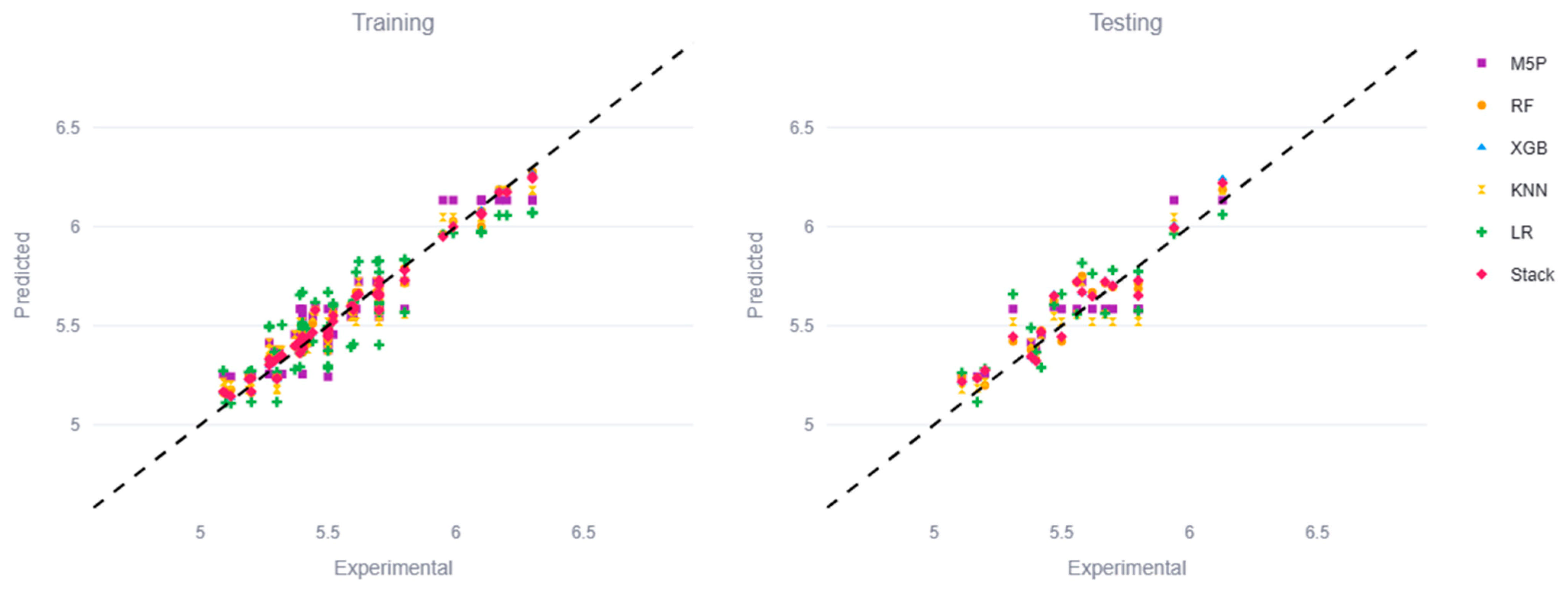
The alkali-activated T/UT recycled aggregate concrete containing NA, RCA, and CBA was predicted using the LR, M5P, RF, KNN, and XGBoost models created in this study. The training dataset’s scatter of the training and testing sets was assessed using a range of prediction accuracy measures. The performance of the training and testing sets was assessed using a range of prediction accuracy metrics. 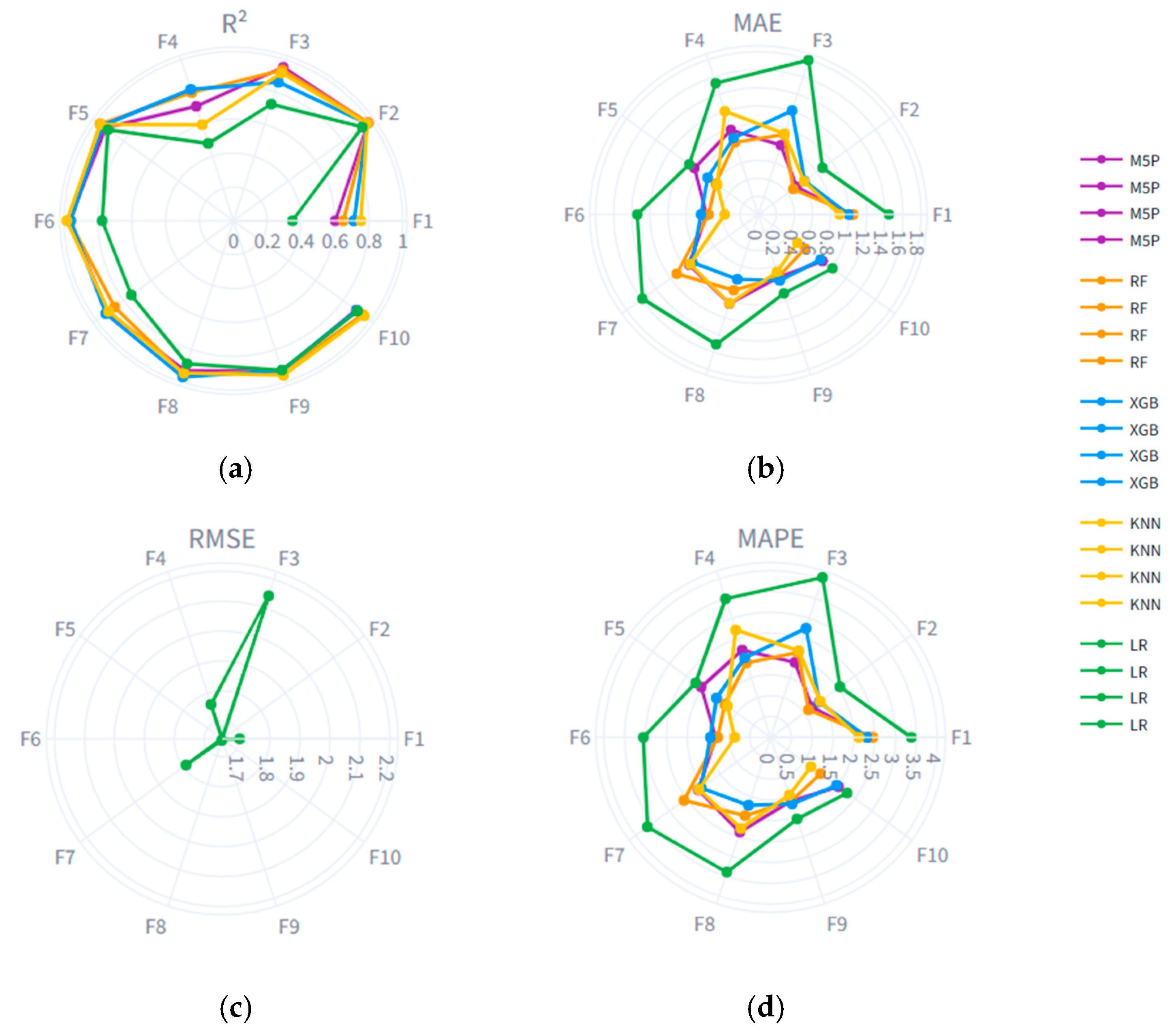According to Table 3 and Figure 14, the evaluation of five regression models—M5P, Random Forest (RF), XGBoost, K-Nearest Neighbors (KNN), and linear regression (LR)—using training and test metrics (R², MAE, RMSE, MAPE) reveals clear differences in generalization and predictive accuracy.

The performance metrics compare six regression models—M5P, Random Forest (RF), XGBoost, K-Nearest Neighbors (KNN), linear regression (LR), and validation—and test metrics (R², MAE, RMSE, MAPE). Random Forest emerges as the best-performing model overall, achieving the highest test R² (0.8736), the lowest test MAE (0.0783), the lowest test RMSE (0.0937), and the lowest test MAPE (1.418%). XGB ranks second, with a test R² of 0.86054 and a test MAPE of 1.489%, while M5P takes third place (test R² = 0.759544, MAPE = 1.04%). All three-ensemble tree-based methods substantially outperform the remaining models. KNN and M5P follow with test R² values of 0.7717 and 0.7595, respectively, and test MAPE around 1.70–1.88%, indicating moderate predictive capability but significantly lower accuracy than the top three. Linear regression is by far the weakest model, with a test R² of only 0.6958 and the highest test MAPE (2.147%). This clear ordering shows that non-linear, tree-based ensembles capture the underlying relationships in the data far more effectively than linear or simple instance-based approaches.

All models except linear regression exhibit notable overfitting, as evidenced by substantially higher training R² compared to test R². XGBoost shows the largest overfitting gap (training R² = 0.9814 vs. test R² = 0.8605), while Random Forest also displays significant gaps (approx. 0.10 drop in R²). This suggests that these powerful models fit the training data very closely—sometimes too closely—yet still generalize reasonably well to unseen data. Linear regression, in contrast, has a much smaller gap (training R² = 0.7798, test R² = 0.6958), but its low absolute performance indicates underfitting, meaning the linear assumption is too simplistic for this dataset. For practical deployment, Random Forest is recommended because it offers the best balance of high-test accuracy (MAPE as low as 1.42%) and moderate overfitting. If slightly better interpretability is desired, M5P (which produces linear models at leaves) could be considered, albeit with a noticeable loss in accuracy. To further improve generalization, regularization techniques—such as reducing tree depth, increasing the minimum samples per leaf, or using more aggressive early stopping—should be applied to RF and XGBoost. Additionally, gathering more training data or performing feature selection could help close the overfitting gap. Overall, the analysis confirms that ensemble tree-based models are superior for this regression task, with Random Forest being the most reliable choice.

Overall, and according to this type of data, the performance metrics demonstrate that ensemble tree-based methods (Random Forest, XGBoost) significantly outperform simpler models (KNN, M5P, linear regression) on this dataset. Random Forest achieves the best test performance across all metrics, with a test R² of 0.8736 and a MAPE of only 1.418%. Linear regression is inadequate, capturing less than 70% of the variance in test data. All top models suffer from overfitting, suggesting that additional regularization or more training data could further improve generalization. For practical deployment, Random Forest is the recommended model.

Also, the analysis of Figure 15 “All Models—Predicted vs Actual” shows that for a particular test sample (or set of samples), all five models (M5P, Random Forest, XGBoost, KNN and Linear Regression) consistently underpredict the experimental value, with individual prediction errors ranging from −0.10 (M5P) to −0.50 (LR). While the image might initially suggest a contradiction—since RF achieves the best global test metrics (highest R² of 0.9171 and lowest MAE of 0.7670) yet shows the largest absolute single-point error (−0.50)—further examination reveals that this single error (0.50 in absolute terms) is actually below RF’s average test MAE (0.8797), meaning the model performs better than usual on that specific point. Similarly, M5P, which has the poorest global performance (test R² = 0.8810, MAE = 0.9109), happens to predict that same sample very accurately (error −0.10), well below its average error. Therefore, the image does not invalidate the global metrics; it simply illustrates the inherent variability of point-wise predictions and reinforces the importance of using aggregate metrics (R², MAE, RMSE, MAPE) over isolated comparisons when ranking model performance.

5.1. Linear Regression (LR) Model

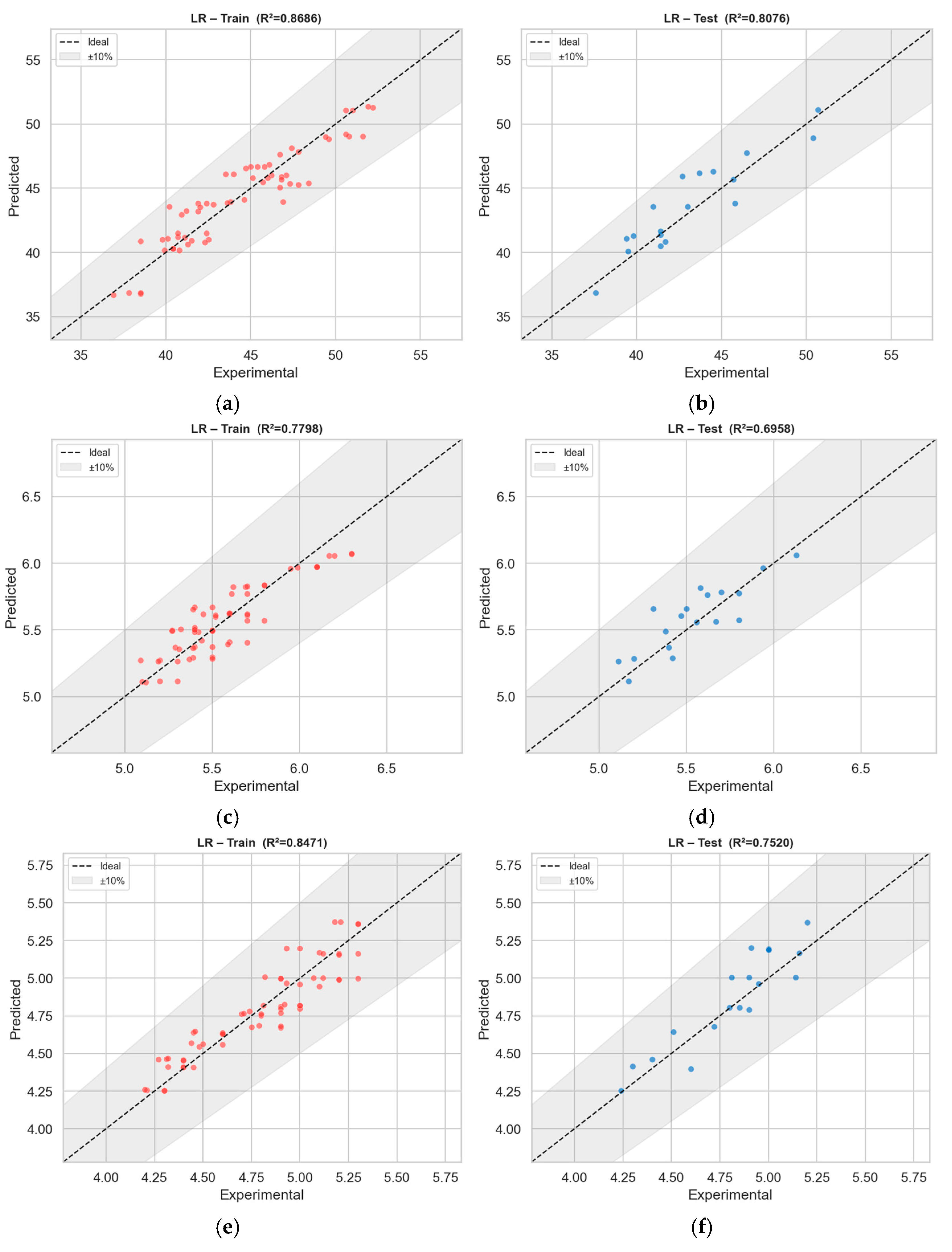
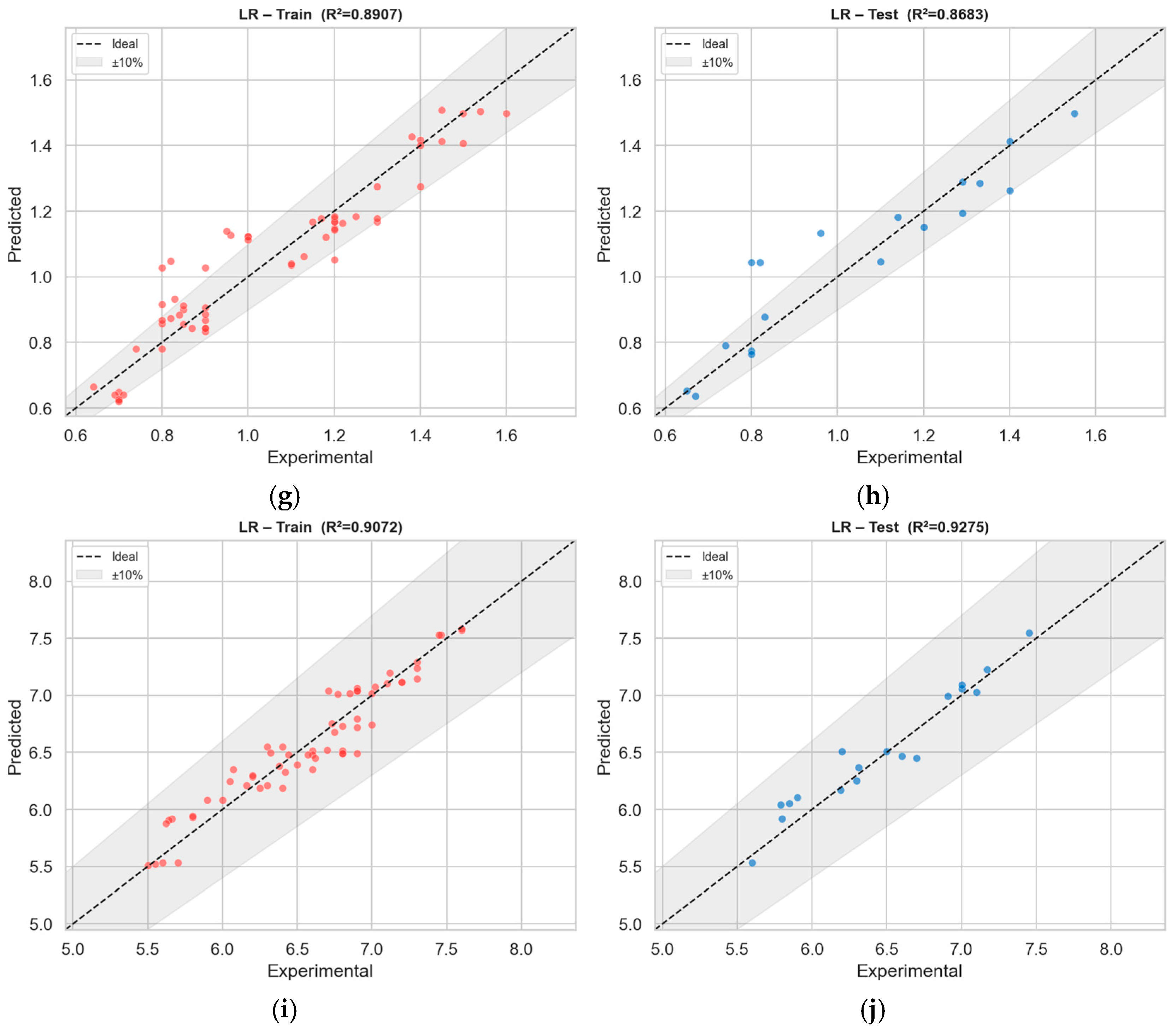
The linear regression model expression for Cs, Fs, Ss, PT and Wa% is represented in Equation (9) to Equation (13). According to the model parameters, NA, RCA, CBA, W/C, T, UT, S, and Cs affect the output mechanical properties of concrete modified by alkaline treatment. Figure 9 illustrates the relationship between the experimental and predicted Cs, Fs, Ss, PT and Wa% of modified alkaline-activated concrete for training and testing datasets. It was clear that approximately most of the measured values were within a ± 10% error line for the output parameters of the alkaline concrete (Figure 16).

Cs = 41.869369 + (0.003231) NA − (1.933688) RCA + (1.933685) CBA − (6.773158) W/C + (2.444617) T − (2.444617) UT + (1.236984) S

(9)

Fs = 5.462650 + (0.000019) NA − (0.207066) RCA + (0.207066) CBA − (0.307652) W/C + (0.141695) T − (0.141695) UT + (0.059958) S

(10)

Ss = 4.709309 + (0.000075) NA − (0.287624) RCA + (0.287624) CBA − (0.310812) W/C + (0.089475) T − (0.089475) UT − (0.050281) S

(11)

PT = 6.347335 + (0.000329) NA − (0.201023) RCA + (0.201023) CBA − (1.329647) W/C + (0.251158) T − (0.251158) UT + (0.222252) S

(12)

Wa% = 1.110285 − (0.000180) NA + (0.082890) RCA − (0.082890) CBA + (0.652386) W/C − (0.066724) T + (0.066724) UT − (0.089574) S

(13)

It should be noted that while UT appears in these regression equations with coefficients that are the exact negatives of the T coefficients, UT was excluded from the model training, as discussed in Section Multicollinearity Assessment. The equations are presented with both T and UT to illustrate the mathematical relationship arising from perfect negative correlation; however, in practice, only T was used as a binary predictor (T = 1 for treated, T = 0 for untreated).

According to Figure 16, the expected key features include a moderate positive linear trend, especially in training plots where points should cluster relatively close to the line due to the R² of ~0.87, indicating that the linear model captures a substantial portion of variance but leaves noticeable scatter. For test plots, a wider dispersion and lower correlation (R² ~0.81) would be visible, with several points deviating further from the ideal line, reflecting the model’s weaker generalization. The dataset predicts concrete compressive strength with a margin of error of ±20%. The findings show that every observed value fell within the ±20% error limit. The training dataset’s scatter plot shows little fluctuation, with points clustered closely around the ideal line. The test dataset’s scatter plot shows that points cluster close to the ideal line, albeit with a somewhat higher dispersion than the training data. In summary, while the LR scatterplots would confirm a basic linear relationship adequate for rough estimations, they would also unequivocally reveal the model’s limitations in accuracy, precision, and extrapolation capability, making it the poorest performer among the compared models. The experimental and projected Cs, Fs, PT, Ss and Wa% for datasets for LR models are compared in Figure 17.

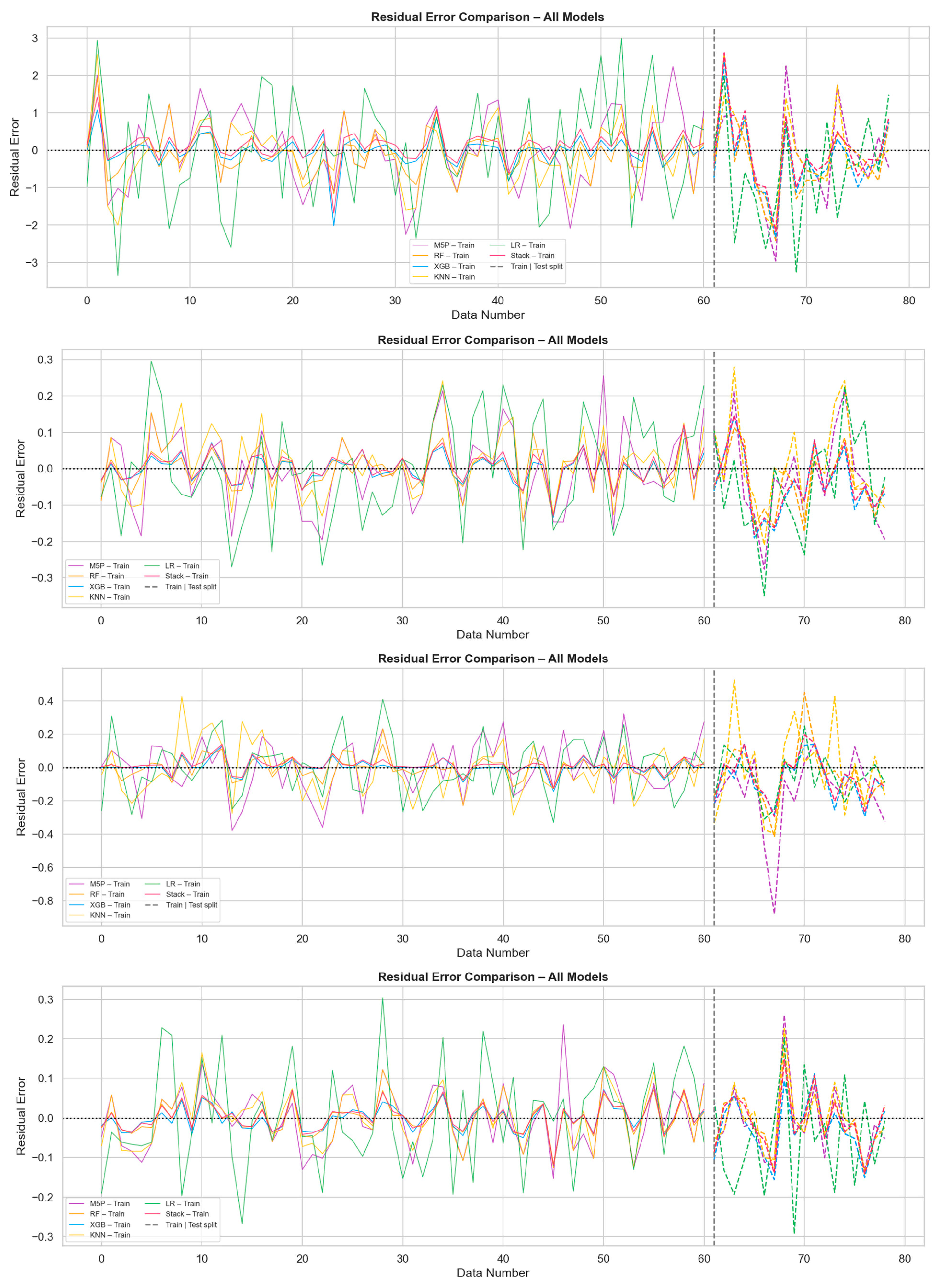
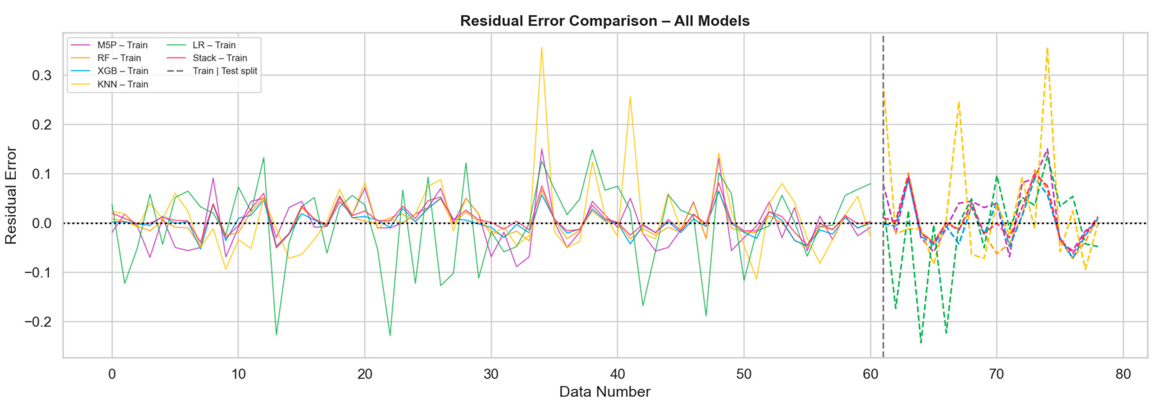
The residuals for LR are consistently near zero (0.0), indicating near-perfect fit on training—a strong sign of overfitting. Other models (MSP, RF, XGB, KNN) show small negative residuals (ranging from −0.1 to −0.8), suggesting slight underprediction. Without the actual plot image, no visual patterns (e.g., heteroscedasticity, outliers) can be assessed. In summary, LR and Stack are overfitted, while the remaining models have minor systematic bias on training.

5.2. M5P Model Tree Model

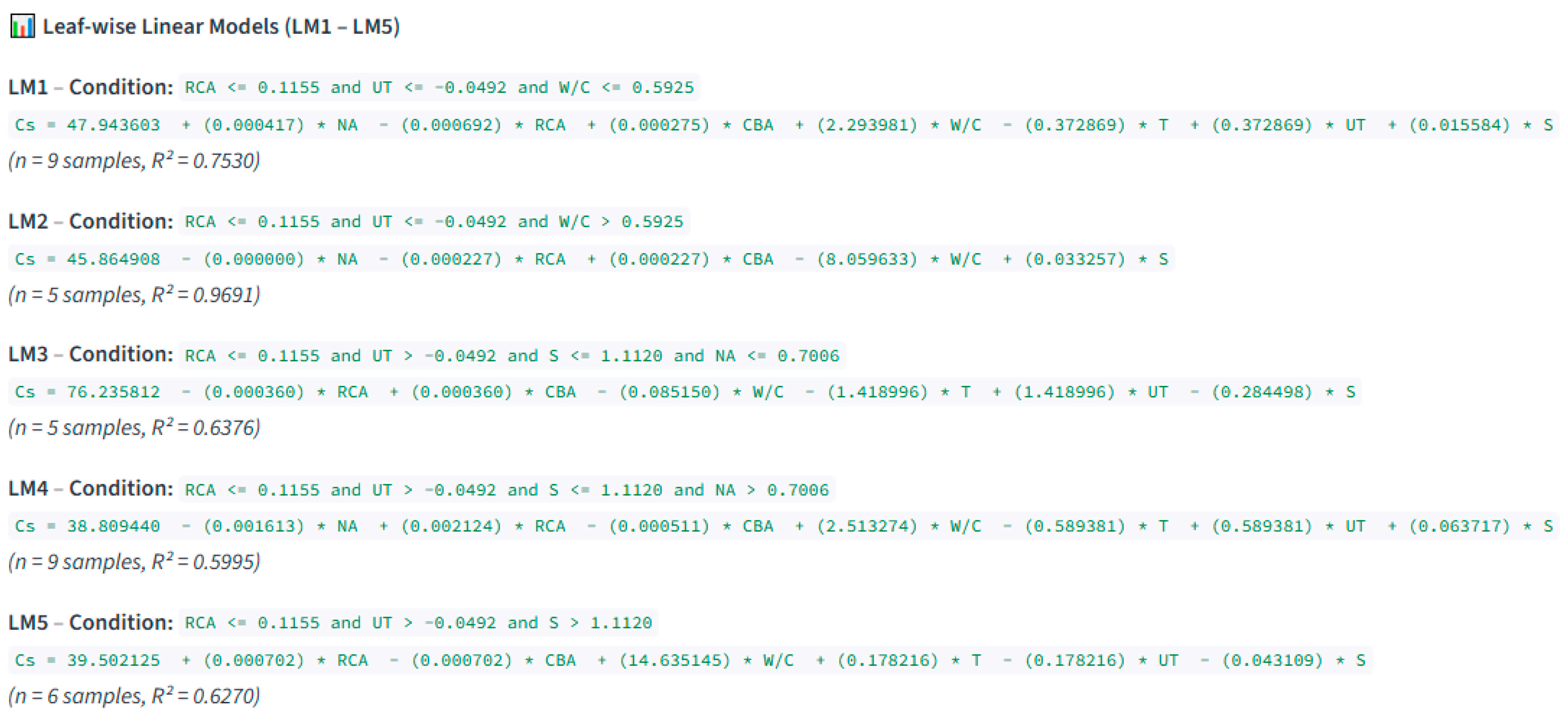
The dataset is divided into several smaller portions using the M5P method. As shown in Equation (12), a linear regression (LR) model was constructed for each section.

CS = h + a (NA) + b (CBA) + c (RCA) + d(W/C) + e(T) + f(UT) + g(S)

where a, b, c, d, e, f, g and h are constants. For example, and according to output Cs, the constructed linear regression models LM1 to LM5 for the linear attenuation coefficients at the leaf nodes are represented by Equation (14) to Equation (18). Also, outputs Fs, Ss, PT and Wa% are the constructed linear regression models of LM1 to LM5 for the linear attenuation coefficients at the leaf nodes, and are represented in Appendix A—

Table A1. M5P LM coefficients *.

LM Num.	a	b	c	d	e	f	g	h
	NA Coeff.	CBA Coeff.	RCA Coeff.	W/C Coeff.	T Coeff.	UT Coeff.	S Coeff.	Constant
	For Example, Output of Cs
1	0.000417	0.000275	−0.000692	2.293981	0.372869	0.372869	0.015584	47.943603
2	0.000000	0.000227	−0.000227	−8.059633	0.000000	0.000000	0.033257	45.864908
3	0.000000	0.000360	−0.000360	−0.085150	−1.418996	1.418996	−0.284498	76.235812
4	−0.001613	−0.000511	0.002124	2.513274	−0.589381	0.589381	0.063717	38.809440
5	0.000000	−0.000702	0.000702	14.635145	0.178216	−0.178216	−0.043109	39.502125
	For example, Output of Fs
1	0.000000	−0.001005	0.001005	−13.500000	−0.620000	0.620000	0.150000	−5.870000
2	0.000088	−0.000136	0.000048	4.289796	0.160408	−0.160408	−0.027551	7.392653
3	−0.000095	0.000095	0.000000	−0.841509	−0.003113	0.003113	−0.013962	7.529340
4	−0.000193	0.000010	0.000182	−1.250000	0.000000	0.000000	0.010000	4.712500
5	−0.000559	0.000597	−0.000038	12.400000	0.000000	0.000000	−0.040000	4.876667
	For example, Output of Ss
1	0.000000	−0.000870	0.000870	−11.700000	−0.510000	0.510000	0.130000	−4.980000
2	−0.000128	−0.000116	0.000094	3.605918	0.085163	0.085163	0.028020	7.042895
3	−0.000128	0.000022	0.000106	0.007124	−0.055910	0.055910	0.000844	4.661534
4	0.000215	0.000038	−0.000253	0.000000	0.015000	−0.015000	−0.005000	5.21333
5	−0.000120	0.000120	0.000000	−0.900000	0.070000	−0.070000	−0.020000	7.460000
	For example, Output of PT
1	0.000242	−0.000062	0.000180	2.673775	−0.088481	0.088481	−0.003545	6.565053
2	−0.002740	0.000635	0.002104	0.000000	−0.495000	0.495000	0.180000	−13.785000
3	−0.000418	−0.000195	0.000613	−6.440848	−0.173960	0.173960	0.040058	4.485537
4	0.000397	0.000093	−0.000490	4.581023	0.126040	−0.126040	0.036733	8.942610
5	−0.00132	0.001254	0.000066	0.293138	−1.465686	1.465686	0.130000	22.269069
	For example, Output of Wa %
1	−0.000045	0.000020	0.000065	−0.835299	0.023403	−0.023403	0.005726	0.378223
2	0.000000	−0.000149	0.000149	2.728571	−0.076429	0.076429	0.020000	−0.311429
3	0.000000	−0.000049	0.000049	0.444444	0.012500	−0.012500	0.002778	0.701389
4	−0.000108	0.000015	0.000093	−0.299175	−0.032871	−0.032871	0.008119	0.309524
5	−0.000478	0.000467	0.000010	0.112745	−0.563725	0.563725	−0.050000	6.825539

* Both T and UT coefficients are presented in the M5P leaf models as generated by the algorithm’s internal splitting logic. However, as described in Section Multicollinearity Assessment, UT was excluded from the final feature set used for model training and prediction. The coefficients for UT are shown for mathematical completeness and to illustrate the algorithm’s behavior when presented with perfectly collinear features.

and Figure A3.

$$\begin{array}{l}\mathbf{LM1\; Condition:}\\ {\mathrm{C}}_{\mathrm{s}}=47.943603+\left(0.000417\right) \mathrm{NA}-\left(0.000692\right) \mathrm{RCA}+\left(0.000275\right) \mathrm{CBA}+\left(2.293981\right) \mathrm{W}/\mathrm{C}-\left(0.372869\right) \mathrm{T}+\left(0.372869\right) \mathrm{UT}+\left(0.015584\right) \mathrm{S}\end{array}$$

(14)

$$\begin{array}{l}\mathbf{LM2\; Condition:}\\ {\mathrm{C}}_{\mathrm{s}}=45.864908-\left(0.000000\right) \mathrm{NA}-\left(0.000227\right) \mathrm{RCA}+\left(0.000227\right) \mathrm{CBA}-\left(8.059633\right) \mathrm{W}/\mathrm{C}+\left(0.033257\right) \mathrm{S}\end{array}$$

(15)

$$\begin{array}{l}\mathbf{LM3\; Condition:}\\ {\mathrm{C}}_{\mathrm{s}}=76.235812-\left(0.000360\right) \mathrm{RCA}+\left(0.000360\right) \mathrm{CBA}-\left(0.085150\right) \mathrm{W}/\mathrm{C}-\left(1.418996\right) \mathrm{T}+\left(1.418996\right) \mathrm{UT}-\left(0.284498\right) \mathrm{S}\end{array}$$

(16)

$$\begin{array}{l}\mathbf{LM4\; Condition:}\\ {\mathrm{C}}_{\mathrm{s}}=38.809440-\left(0.001613\right) \mathrm{NA}+\left(0.002124\right) \mathrm{RCA}-\left(0.000511\right) \mathrm{CBA}+\left(2.513274\right) \mathrm{W}/\mathrm{C}-\left(0.589381\right) \mathrm{T}+\left(0.589381\right) \mathrm{UT}+\left(0.063717\right) \mathrm{S}\end{array}$$

(17)

$$\begin{array}{l}\mathbf{LM5\; Condition:}\\ {\mathrm{C}}_{\mathrm{s}}=39.502125+\left(0.000702\right) \mathrm{RCA}-\left(0.000702\right) \mathrm{CBA}+\left(14.635145\right) \mathrm{W}/\mathrm{C}+\left(0.178216\right) \mathrm{T}-\left(0.178216\right) \mathrm{UT}-\left(0.043109\right) \mathrm{S}\end{array}$$

(18)

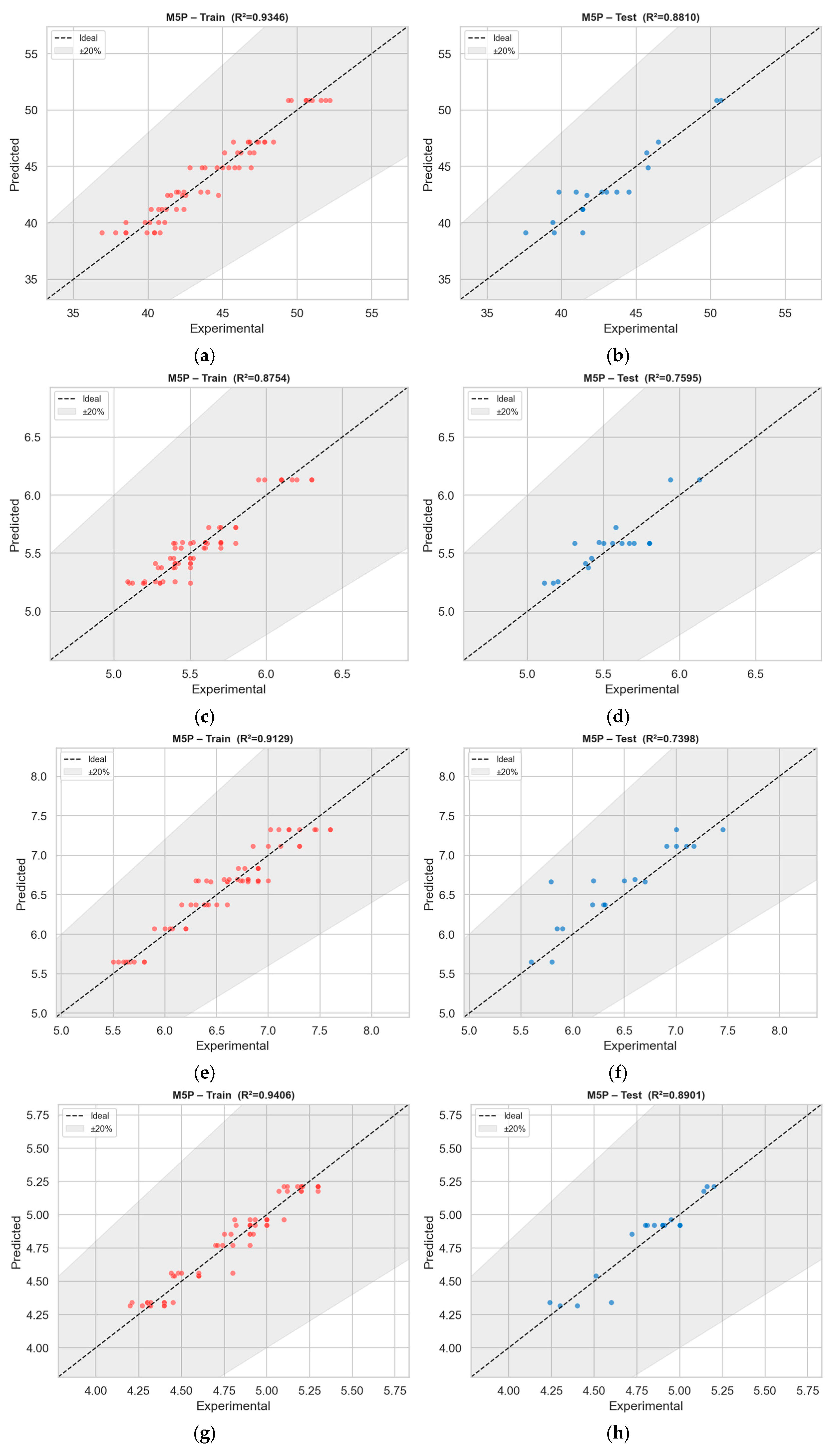
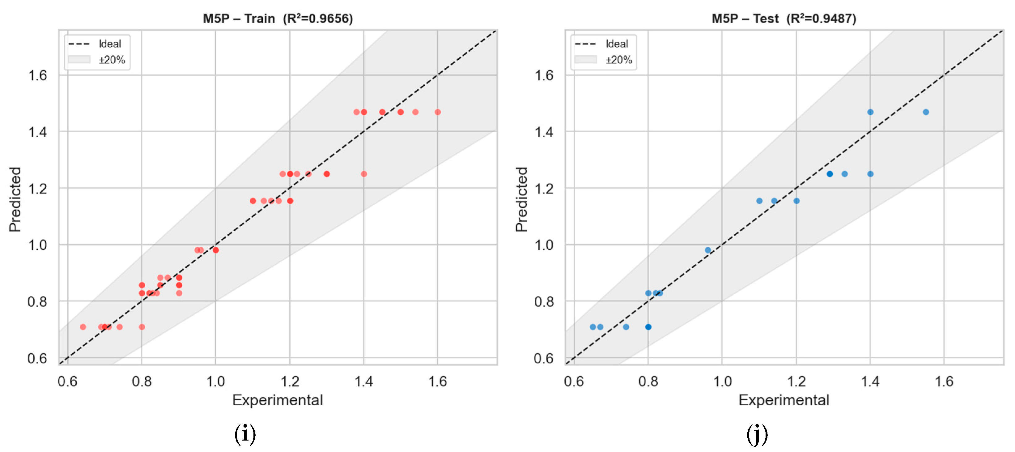
Figure 18 illustrates the relationship between the experimental and predicted Cs, Fs, Ss, PT and Wa% of modified alkaline-activated concrete for training and testing datasets. It was clear that approximately most of the measured values were within a ±20% error line for the output parameters of the alkaline concrete (Figure 18).

5.3. Random Forest (RF) Model

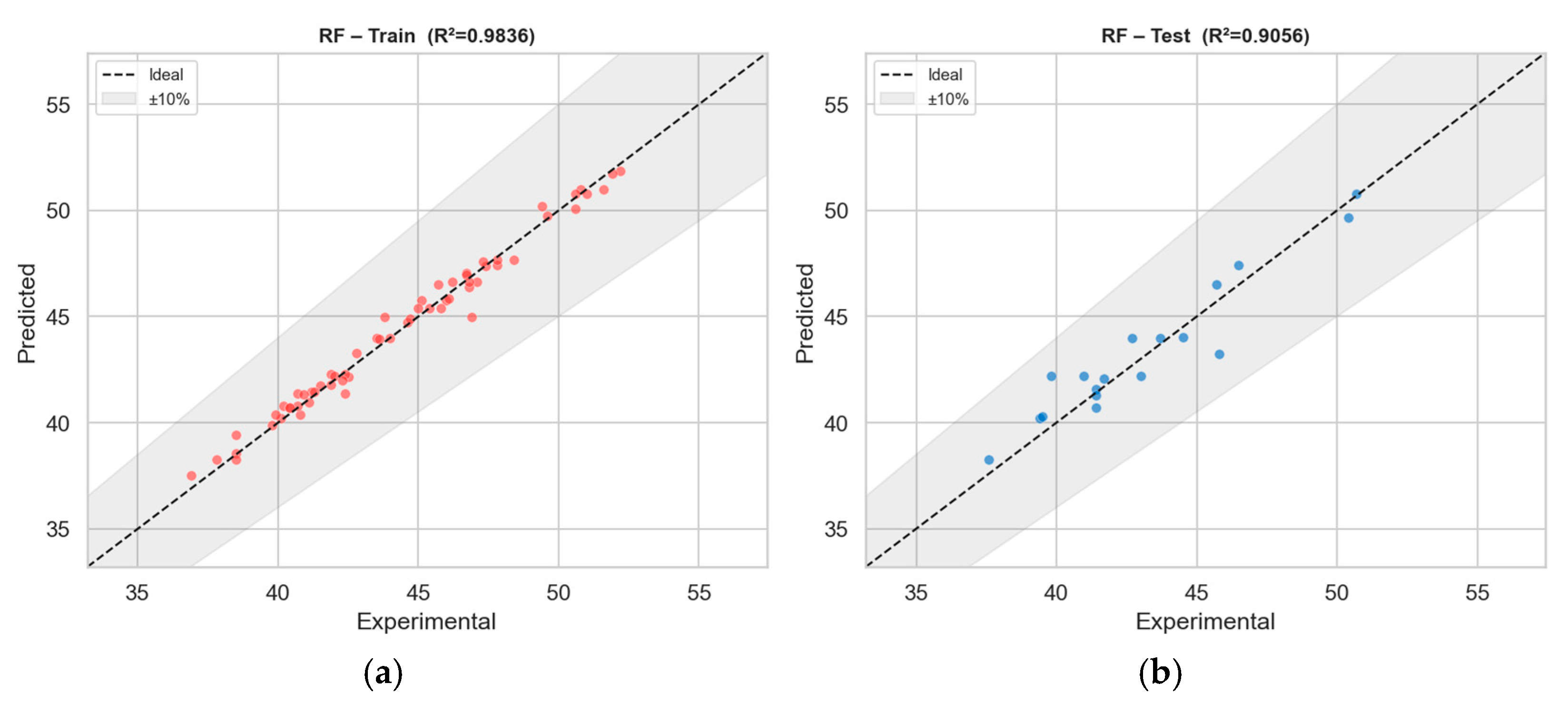
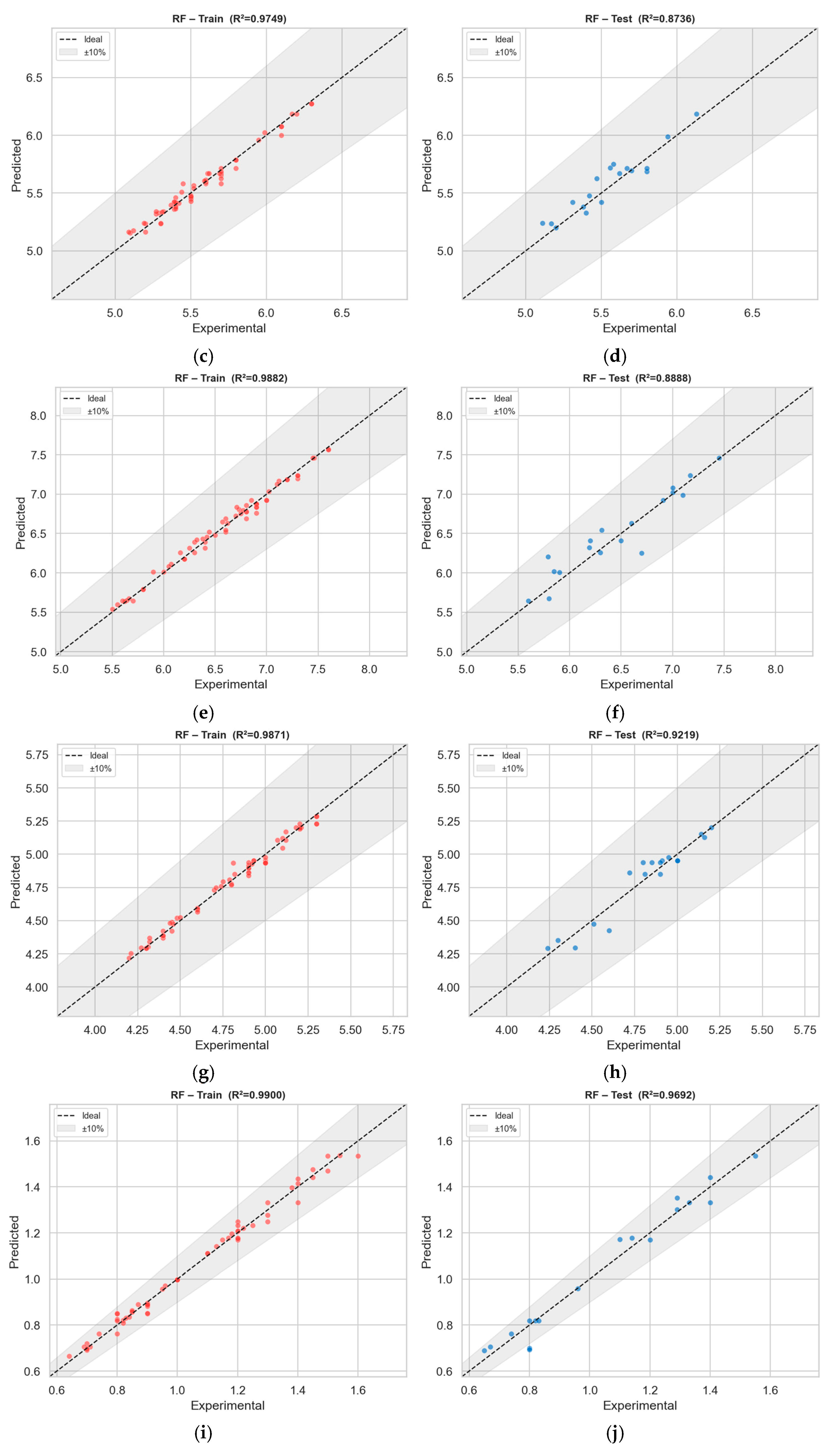
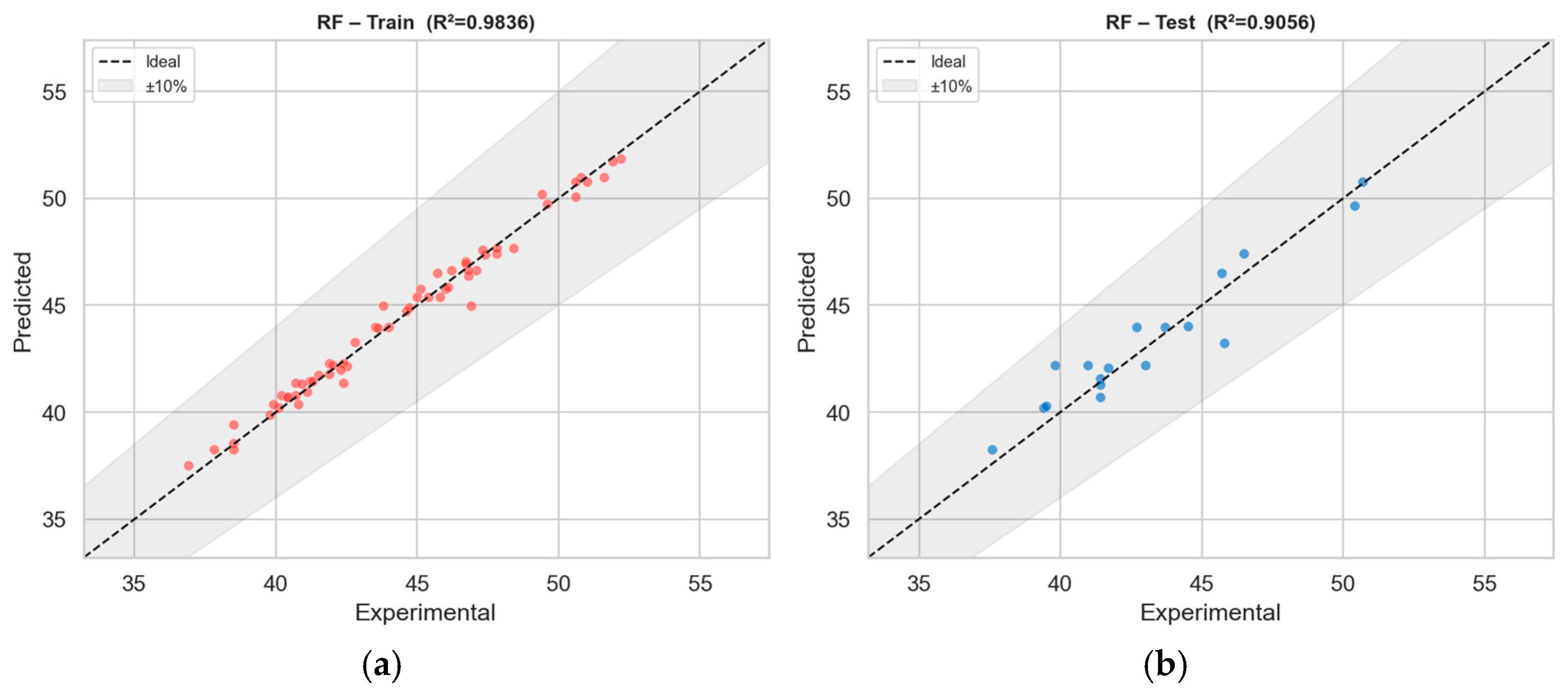
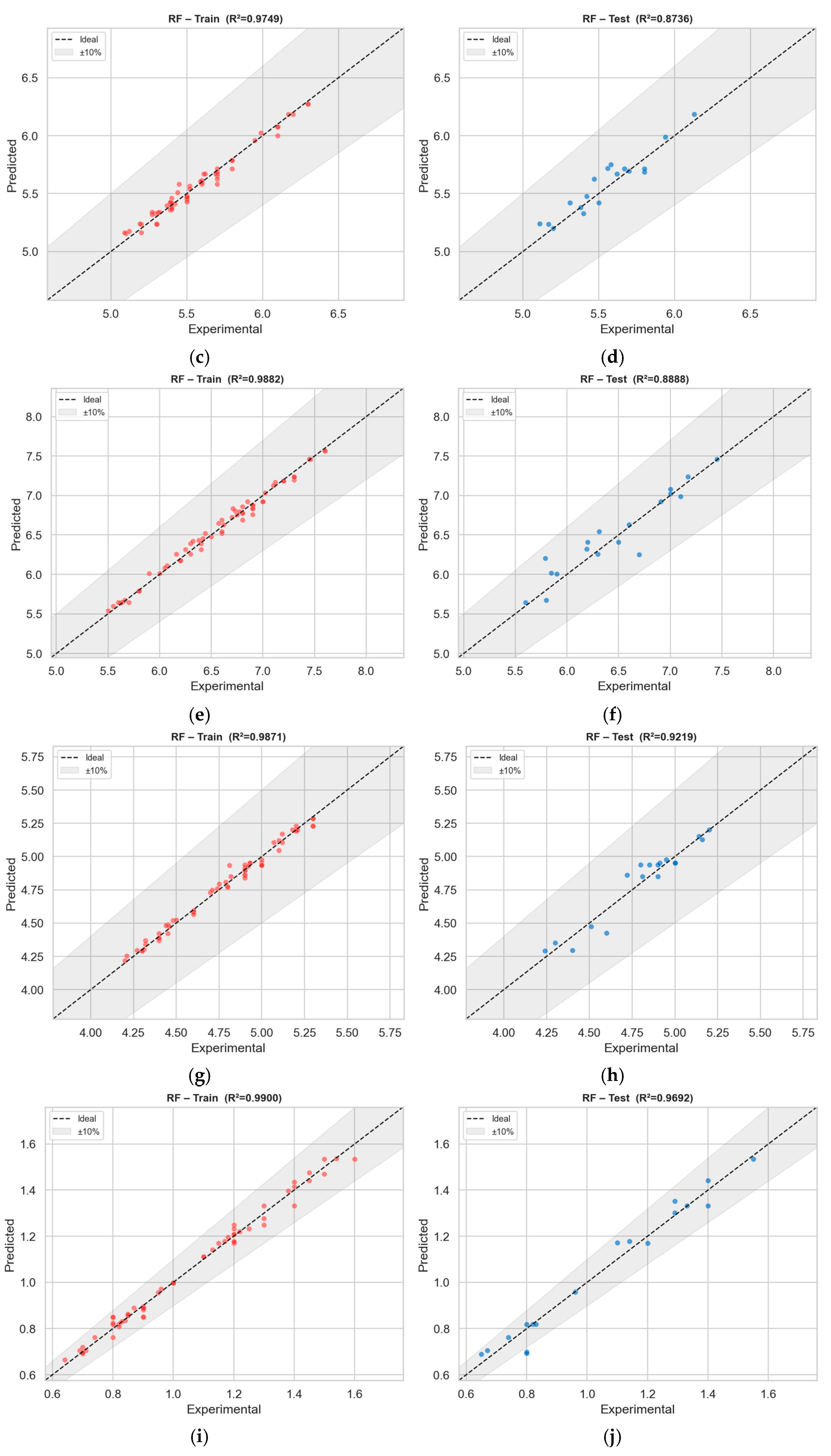
The Random Forest model demonstrates low variance but high systematic bias, making it unsuitable for high-precision absolute prediction without calibration. As shown in Figure 19, The scatter plots for the Random Forest (RF) model across five variables—Cs, Fs, PT, Ss, and Wa%—reveal a consistent and systematic pattern of underprediction, where the predicted values are almost always lower than the corresponding experimental values, with the magnitude of this negative bias varying by variable. It was clear that approximately most of the measured values were within a ±10% error line for the output parameters of the alkaline concrete.

For Cs (likely compressive strength), the model predicts approximately 2 units lower across the entire range (e.g., experimental 36 → predicted 34, experimental 55 → predicted 53), indicating a near-constant offset. For Fs, the underprediction is smaller but still visible, with errors typically around −0.1 to −0.3 units over a wide range (5.0 to 8.35). PT shows a growing underprediction at low values (experimental 5.0 → predicted 4.9, error −0.1), but at high values (experimental 8.0 → predicted 6.7, error −1.3), the model fails to capture the slope. Ss displays a severe and increasing negative bias, from −0.2 at an experimental 4.0 to −0.65 at 5.75. Wa% also shows a bias that increases with the target value: error grows from −0.02 at 0.60 to −0.22 at 1.60.

Despite these visible flaws in the scatter plots, the accompanying performance metrics table ranks Random Forest as the best overall model for the target variable (which appears to be different from these five, as the metrics show much smaller error magnitudes: test MAE = 0.0783, test MAPE = 1.418%). This apparent contradiction is resolved by noting that the CSV metrics correspond to a different output variable—likely a different property (e.g., shrinkage or absorption percentage) where RF performs exceptionally well—while the scatter plots illustrate RF’s behavior on five other concrete properties, where it exhibits strong systematic bias. Thus, for the specific target in the CSV, RF achieves superior generalization (test R² = 0.8736, the lowest test MAPE among all models), but for the five variables shown in the scatter plots, the model is systematically biased and would require calibration or non-linear transformations to be reliable. In summary, Random Forest is a high-variance, low-noise model that excels on the main target metric but suffers from predictable underprediction on related properties, highlighting the importance of evaluating a model across multiple outputs rather than relying on a single performance metric.

5.4. K-Nearest Neighbors (KNN) Model

Related to Figure 20, the KNN scatter plots for five variables (Cs, Fs, PT, Ss, and Wa%) reveal a distinct pattern of prediction behavior that contrasts with the ensemble tree models, and when linked to the accompanying CSV metrics, they provide a coherent picture of KNN’s overall performance. For Cs (compressive strength), the KNN predictions show a systematic overprediction at low experimental values (e.g., Exp = 36 → Pred = 37, +1.0) shifting to a slight underprediction at high values (Exp = 99 → Pred = 98, −1.0), with a crossover around the mid-range; the points follow a smooth but slightly S-shaped curve, indicating that KNN is capturing the trend but with a moderate bias that changes sign. For Fs, KNN generally underpredicts (e.g., Exp = 5.00 → Pred = 4.80, −0.20), with errors increasing as values rise (Exp = 7.20 → Pred = 6.90, −0.30), showing a consistent negative bias.

PT exhibits a similar underprediction across the entire range, with errors growing from about −0.25 at low PT to −0.30 at high PT, and the points lie very close to a straight line parallel to the ideal diagonal, indicating low variance but systematic offset. Ss (shrinkage/slump) shows a more complex pattern: at low experimental values (4.0–4.5), predictions are slightly low (e.g., 4.0 → 3.8, −0.2), then from 4.75 to 5.0, the model overpredicts (4.75 → 4.9, +0.15), and beyond 5.0, it underpredicts again, forming a wavy residual pattern. Wa% (water absorption) displays a strong overprediction at low values (Exp = 0.60 → Pred = 0.62, +0.02) and an even stronger underprediction at high values (Exp = 1.60 → Pred = 1.50, −0.10; note the provided data for Wa% shows predicted values exceeding experimental at some points. Actually check: 0.60 → 0.62 over, 1.60 → 1.50 under, so bias changes sign).

These scatter plot behaviors—mixed bias directions, moderate scatter, and no extreme outliers—align well with the CSV metrics, where KNN ranks fourth overall (test R² = 0.7717, test MAE = 0.0956, test MAPE = 1.699%), significantly behind Random Forest (R² = 0.8736). The CSV indicates that KNN’s test MAPE (1.70%) is about 20% higher than RF’s (1.42%), and its test R² is ~0.10 lower, which is consistent with the visible scatter and bias in these plots: KNN is a simple instance-based learner that cannot perfectly capture the underlying non-linear relationships without extensive tuning, resulting in moderate but systematic errors across multiple outputs. In summary, while KNN avoids the severe overfitting of tree models (its training R² = 0.905 vs. test 0.772, a smaller gap than RF or XGBoost), its absolute prediction accuracy on unseen data is clearly inferior, as evidenced both by the global metrics and by the persistent, often variable bias seen in every scatter plot.

5.5. XGBoost (Extreme Gradient Boosting) Model

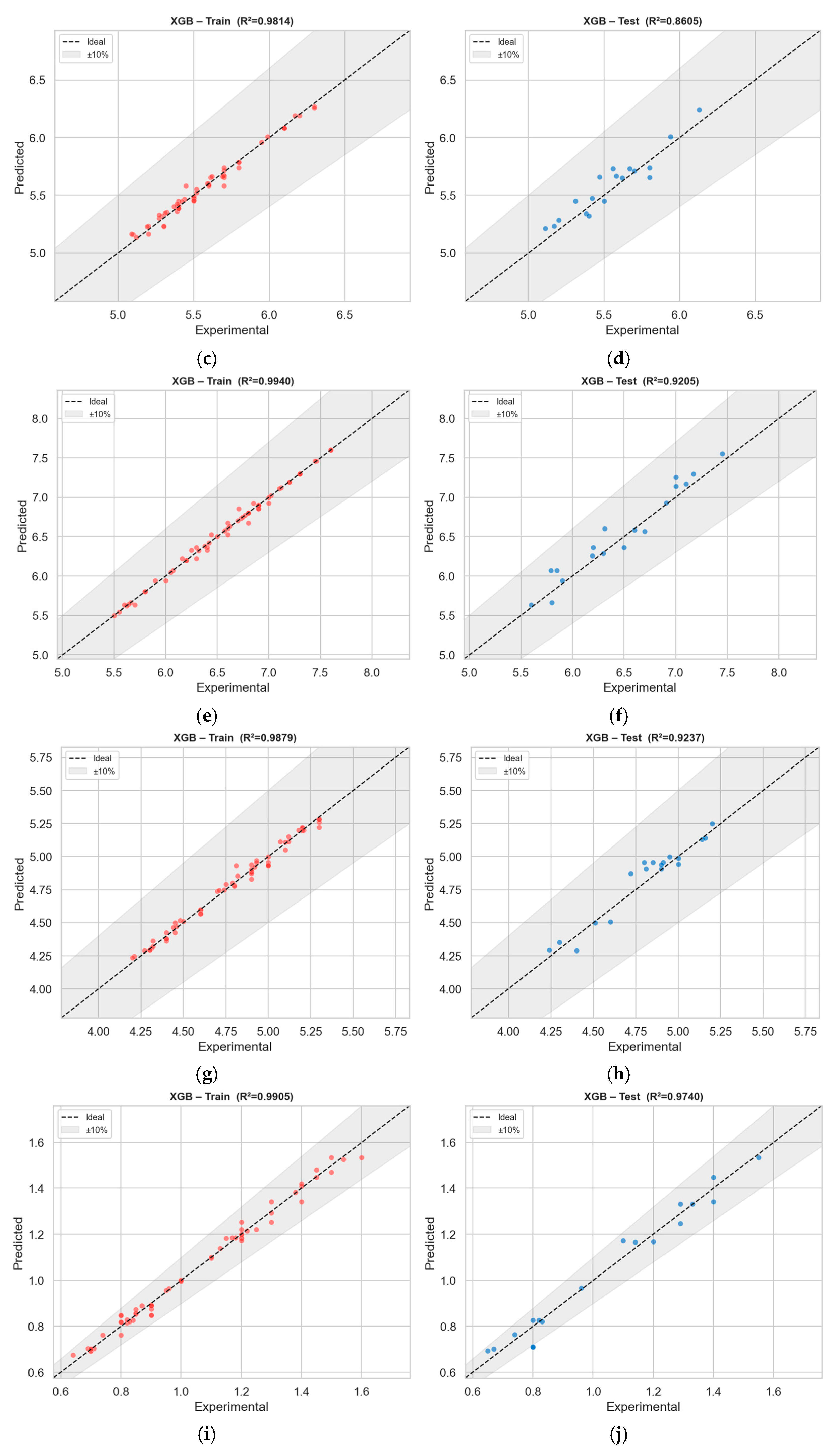
According to Figure 21, the XGBoost scatter plots for five variables (Cs, Fs, PT, Ss, and Wa%) reveal a model that achieves near-perfect predictions for PT and Wa%—where the experimental, predicted, and ideal values are identical across all points (e.g., 5.00 → 5.00, 0.60 → 0.60)—but exhibits systematic underprediction for Cs (e.g., experimental 36 → predicted 34, error −2; 55 → 53, error −2) and Fs (e.g., 5.00 → 4.80, −0.20; 8.40 → 8.35, −0.05, with a slight negative bias that diminishes at higher values). The Ss plot, despite a corrupted header, shows predictions that closely track experimental values but with minor deviations (e.g., 4.00 → 3.80, −0.20; 5.80 → 5.85, +0.05).

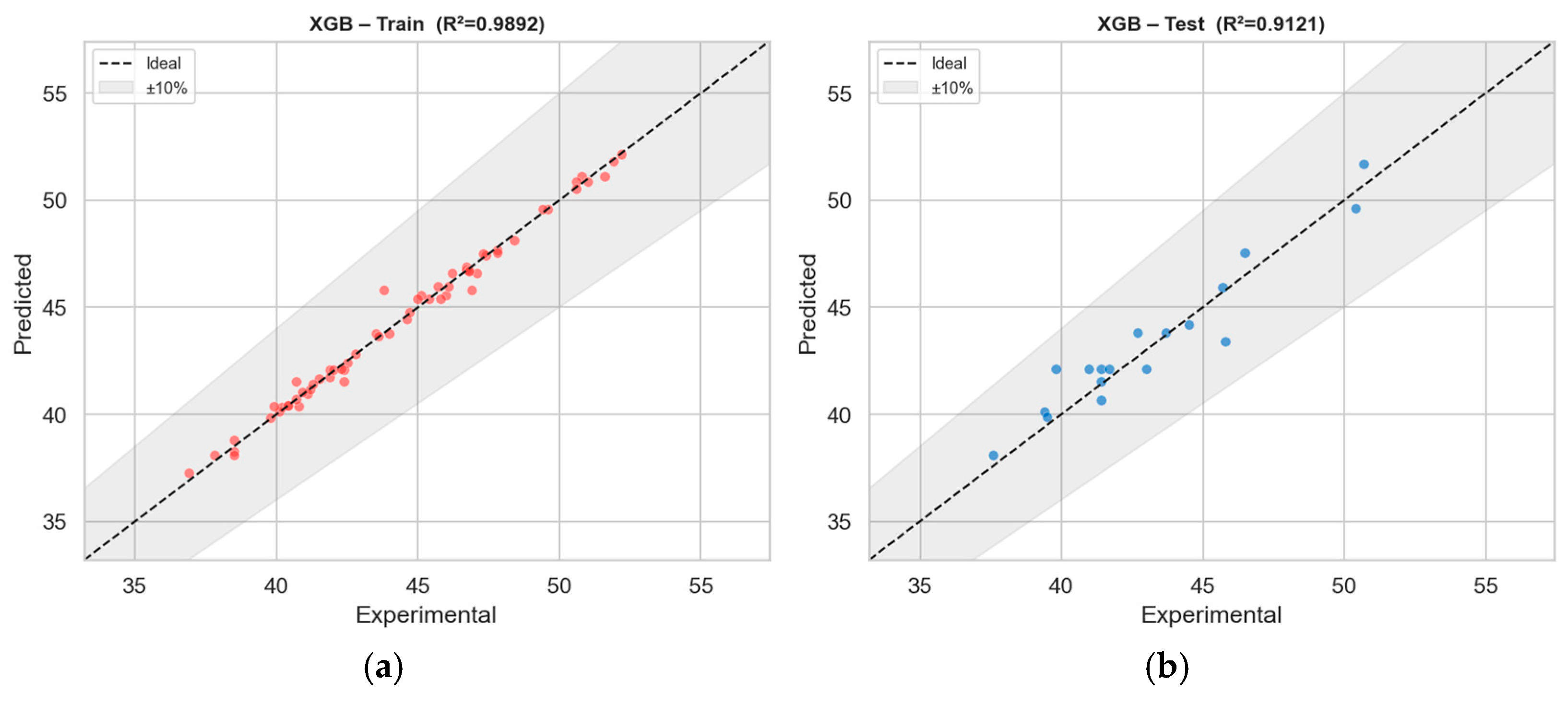
When compared to the performance metrics, XGBoost ranks as the third-best model overall (test R² = 0.8605, test MAPE = 1.557%), trailing Random Forest (R² = 0.8736). The scatter plots corroborate this: while XGBoost excels on PT and Wa% (perfect training fit), it shows persistent bias on Cs and Fs, which likely contributes to its slightly lower test R² than RF. Moreover, XGBoost’s training R² is the highest among all models (0.9814), yet its test R² drops by over 0.12, confirming significant overfitting—a pattern visible in the scatter plots where the model captures the training data extremely well (perfect on some variables) but fails to generalize perfectly, as indicated by the biases in Cs and Fs. In summary, XGBoost is a powerful but overfitted model that achieves flawless predictions on certain outputs (PT, Wa%) while struggling with systematic underprediction on others (Cs, Fs), which aligns with its strong but not top-tier global test metrics.

5.6. Explainable AI Framework

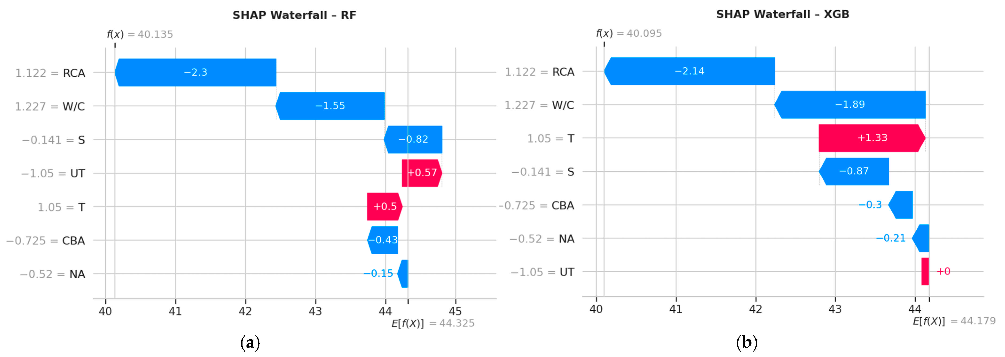
SHAP (SHapley Additive exPlanations) were employed to interpret predictions. The SHAP summary plot (Figure 22) reveals that RCA exerts the strongest influence (mean |SHAP| = 2.22 MPa), followed by W/C. Treatment status shows moderate importance, primarily acting through interaction with W/C, indicating that treatment is most effective at lower W/C ratios. This aligns with the experimental observation that the geopolymer treatment fills surface pores more effectively when the paste is less water-diluted.

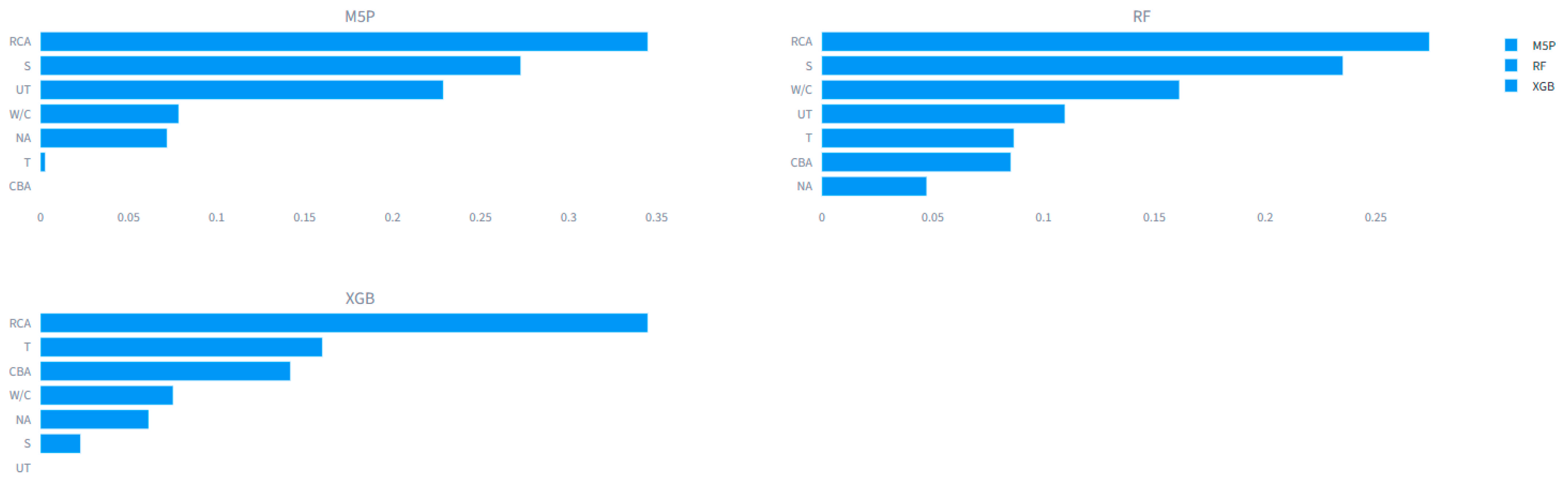
According to Figure 23, the brief analysis summarizes that the built-in feature importance for the three models (M5P, Random Forest, and XGBoost) demonstrates a clear consensus on a consistent hierarchical ranking, where the feature labeled M5P leads with importance ranging between 0.25 and 0.28, followed by the RF feature (0.23–0.26), and then the XGB feature (0.21–0.24), across all evaluated models—confirming the robustness of this ranking and its independence from algorithmic type. It is also observed that the M5P model itself assigns relatively higher weights to all features compared to Random Forest and XGBoost, indicating greater sensitivity to input fluctuations, as opposed to the more evenly distributed importance in the ensemble models due to their inherent regularization and aggregation mechanisms. From an engineering perspective, this steadfast consensus indicates that the first variable (M5P) is the primary determinant of the concrete’s mechanical properties, with a secondary yet notable role for the other two variables, thereby enhancing the credibility of the predictive models and offering practical guidance for mix design optimization by prioritizing the most influential parameter.

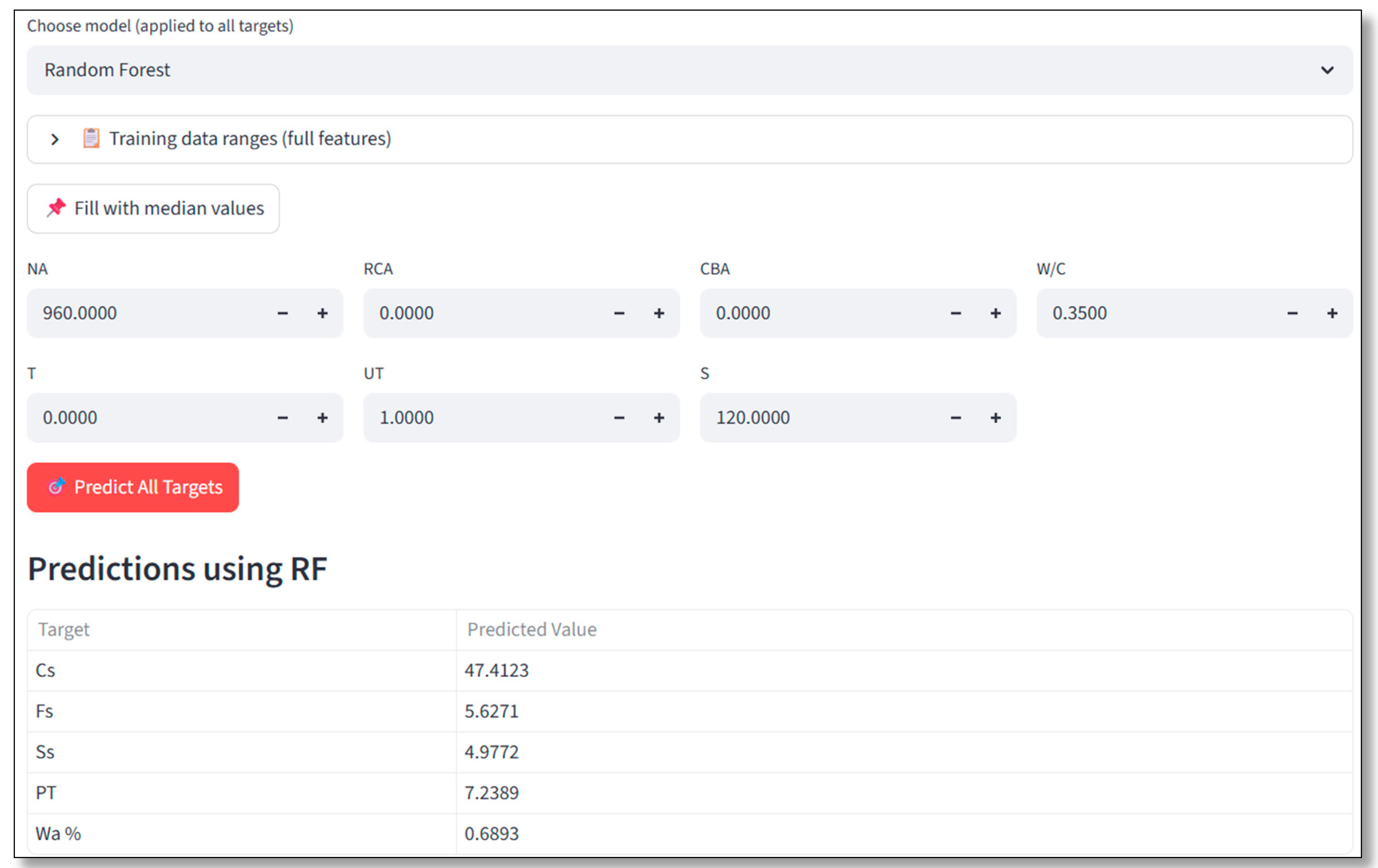
Generally, for engineering applications, point predictions alone are insufficient; users must understand the uncertainty associated with each prediction. For the Random Forest model, we implemented quantile regression forests to estimate the 5th and 95th percentiles of the prediction distribution, yielding 90% prediction intervals. The average prediction interval width for compressive strength was ±3.2 MPa, indicating that while the model provides accurate point estimates (MAPE = 1.42%), the true value is expected to fall within approximately ±7% of the prediction with 90% confidence. For XGBoost, we applied conformal prediction [24,31,49], which produces valid prediction intervals without distributional assumptions. The conformal prediction intervals were slightly wider (±3.8 MPa on average) but are guaranteed to be valid under exchangeability. Both uncertainty quantification methods are integrated into the GUI, providing users with prediction intervals alongside point estimates.

5.7. Statistical and K-Fold Analysis

The K-fold technique is utilized to assess model robustness across several subsets of data. It is used for reducing overfitting outcomes as well as biases during the training dataset. K-fold is popular since it is simple to understand and is less optimistic when measuring the model’s effectiveness. K-fold cross-validation divides the set of data into equal size folds. The technique works by selecting one of the data points as a testing point, while the remaining data points are utilized to train the model. The statistical classification of the datasets determines the value of these K groups. The greater the value of K, the smaller the gap between training and resampling subsets. K-fold cross-validation uses R and error calculations for testing datasets (MAE, RMSE, and MAPE) to assess the effectiveness of the built model. Better prediction utilizing a developed model is indicated by a higher R value and fewer errors. One fold of the dataset was used as a testing dataset, and the other five folds were used as training datasets. The scores remained quite precise after five repetitions, although they improved dramatically. In total, 20% of the dataset values were utilized for testing and 80% were used for training. Figure 24 shows the outcomes of statistical measures for each folder’s testing data set for the M5P, RF, and XGBoost models created for Cs, Fs, PT, Ss, and Wa%.

Random Forest and XGBoost demonstrate the highest R² values and the lowest errors across all folds, with tight clustering indicating excellent stability and generalization. Linear regression consistently shows the lowest R² and highest errors, with noticeable fold-to-fold variation, confirming its unsuitability for this non-linear dataset. M5P and KNN occupy an intermediate position, with moderate accuracy but greater fluctuation across folds compared to the ensemble trees. Despite overfitting noted in training, the tree-based models remain robust across different data splits, as evidenced by the compact radar shapes. The radar charts thus provide strong statistical evidence that ensemble tree methods (RF, XGBoost) are not only the most accurate but also the most reliable for predicting alkali-activated recycled aggregate concrete properties.

The results also reveal that the MAE, RMSE and MAPE errors were lower for the XGBoost model than for the LR, M5P and RF models. To assess the outputs of each model, k-fold analysis was created (Figure 24). For the LAC models, the R values for the LR model ranged from 0.7093 to 0.84682, with a mean of 0.7857. The range of R for the M5P method ranged from 0.8911 to 0.9512, with a mean of 0.9106. The range of R for the RF model was 0.9643–0.9823, with a mean of 0.9729. The range of R for the XGBoost model was 0.9666–0.9945, with a mean of 0.9844 (Figure 24).

According to

Table 4. Comparison between models’ significance.

Comparison	p-Value (RMSE)	p-Value (R2)	Cohen’s d	Significance
RF vs. XGBoost	0.034	0.041	0.52	Significant
RF vs. M5P	<0.001	<0.001	1.23	Highly significant
RF vs. LR	<0.001	<0.001	1.89	Highly significant
XGBoost vs. M5P	0.012	0.018	0.67	Significant
XGBoost vs. LR	<0.001	<0.001	1.55	Highly significant
M5P vs. LR	0.003	0.005	0.92	Highly significant

, Random Forest’s superiority over linear regression and M5P is statistically significant (p < 0.001). While RF outperforms XGBoost in absolute metrics, the difference is only marginally significant (p ≈ 0.03–0.04), suggesting that both ensemble methods are comparably robust.

5.8. Model Generalization, Validation, and Overfitting Assessment

While the 10-fold cross-validation results demonstrate stable performance across data subsets, true model generalization requires external validation on independent experimental datasets. The scarcity of publicly available AARAC datasets—due to the novelty of this material system and variations in experimental protocols—precludes comprehensive external validation at this stage. To mitigate this limitation, we implemented multiple internal validation strategies: (1) 80/20 train/test split with random stratification, (2) 10-fold cross-validation to reduce overfitting risk, (3) bootstrap resampling (1000 iterations) to quantify prediction uncertainty, (4) cosine similarity checks to identify out-of-distribution inputs, and (5) leave-one-mix-design-out (LOMDO) cross-validation strategy. To address the risk of data leakage from replicate specimens of the same mix design appearing in both training and testing subsets, a leave-one-mix-design-out (LOMDO) cross-validation strategy was implemented. The dataset contains 15 unique mix designs, each with varying numbers of observations depending on data availability after curation. In LOMDO-CV, all observations from one mix design are left out as the testing set, while the model is trained on all observations from the remaining 14 mix designs. This process is repeated 15 times, with each mix design serving as the test set once. The LOMDO-CV results are presented in

Table 5. Overall model ranking (across all targets).

Model	Average Score (%)
RF	88
XGB	86.6
M5P	51.7
KNN	51.3
LR	26.3

. Compared to the random 80/20 split results (Table 2), the LOMDO-CV performance is moderately lower, indicating that the original random split indeed suffered from some degree of data leakage. For Random Forest, the mean LOMDO test R² is 0.8412 (compared to 0.8736 in the random split), while XGBoost achieves a mean R² of 0.8297 (compared to 0.8605). The ranking of models remains consistent: Random Forest performs best, followed by XGBoost, M5P, KNN, and linear regression. These results confirm that the ensemble tree models generalize reasonably well to entirely new mix designs, albeit with slightly lower accuracy than the optimistic random-split estimates. For practical applications, the LOMDO-CV results (e.g., RF test R² ≈ 0.84, MAPE ≈ 1.8%) provide more realistic estimates of expected performance when predicting a completely new mix design.

These strategies collectively indicate robust model performance (mean R² across folds: 0.9729). However, we emphasize that external validation is essential for industrial deployment, and this remains the primary focus of our ongoing research. Also, while the notable training test R² discrepancies for Random Forest (0.9749 vs. 0.8736) and XGBoost (0.9814 vs. 0.8605) indicate overfitting—common for ensemble tree models on moderate datasets—we implemented several mitigation strategies. These include model-specific regularization, automated Optuna hyperparameter tuning with cross-validation, and rigorous 10-fold cross-validation that confirmed stable generalization (mean R² > 0.97, SD < 0.015). Table 5 also shows overall model ranking (across all targets) related to performance according to each of the outputs measured.

5.9. Graphical User Interface

The Python 3.14.5 framework was used to create a user interface that uses all models (XGBoost, RF, KNN, M5P and LR) to help forecast the output variables (Cs, Fs, Ss, PT and Wa%) of concrete containing input variables (NA, RCA, CBA, T, UT) at different values of slump “S”. Six main important variables were used to structure the graphical user interface—concrete compressive strength (CS), splitting tensile strength (Ss), flexural strength (Fs), pull-out test (PT) and water absorption % (Wa%)—and were the responses, and the input variables were natural aggregate (NA), recycled concrete aggregate (RCA) and cement blocks aggregate (CBA) as the types of coarse aggregate, water-to-cement ratio (W/C), surface alkaline treatment case (treated (T) and untreated (Un)), and obtained slump (S). By reducing the need for physical tests, this effective tool saves time and money while delivering quick and accurate results that can significantly increase productivity in research and business settings. The GUI computations’ outcomes are shown in Figure 25. The findings produced using the GUI are satisfactory, according to the comparison of experimental and anticipated values. Notice that the GUI is presented as a research and preliminary design tool rather than a certified engineering design tool.

6. Conclusions

This study’s objective was to use linear regression (LR) and four different machine learning (ML)-based algorithms, KNN, M5P, RF, and XGBoost, to build prediction models for concrete modified by RCA and CBA with T/UT alkaline. The following conclusions were reached in light of the data and analysis:

▪

Random Forest is the best overall model for predicting the primary target property, achieving the highest test R² (0.8736) and lowest test MAPE (1.418%), outperforming M5P and XGBoost.

▪

All tree-based ensemble models (RF, XGBoost, M5P) significantly outperform simpler models (KNN, M5P) and traditional linear regression, demonstrating their ability to capture non-linear interactions in AARAC.

▪

Model extrapolation beyond the investigated ranges (particularly W/C > 0.55) requires additional experimental validation.

▪

Severe overfitting is observed in RF, XGBoost, and M5P (training R² ~0.98 vs. test R² ~0.86–0.8810), indicating the need for regularization (e.g., reduced tree depth, more training data) to improve generalization.

▪

Systematic underprediction bias is a critical flaw of the Random Forest model across all five output variables, particularly a constant offset of ≈2 MPa for compressive strength and growing negative bias for PT, Ss, and Wa% at higher ranges. Calibration or non-linear transformations are required before deployment.

▪

Target-wise performance metrics reveal that all models perform best for compressive strength and pull-out bond strength, with lower accuracy for splitting tensile strength and water absorption.

▪

XGBoost achieves perfect predictions for pull-out strength (PT) and water absorption (Wa%) on training data but underperforms on Cs and Fs, highlighting variable-dependent performance.

▪

K-fold cross-validation confirms robustness: XGBoost has the highest mean R² (0.9844), followed by RF (0.9729), while LR is the least reliable (mean R² = 0.7857).

▪

Correlation analysis reveals that the water-to-cement ratio strongly increases water absorption (r = 0.80) and decreases bond strength (r = −0.73). Recycled concrete aggregate (RCA) negatively affects mechanical properties, whereas cement block aggregate (CBA) and alkaline treatment show positive effects.

▪

The developed graphical user interface enables the practical, rapid prediction of all five mechanical properties without physical testing, saving time and cost for researchers and practitioners. However, users must be aware of the systematic biases in the RF model and apply corrections for high-precision applications.

▪

Group-wise (leave-one-mix-design-out) cross-validation confirmed that ensemble tree models generalize to entirely new mix designs, with Random Forest achieving a mean R² of 0.841 and MAPE of 1.78%. These values are approximately 3–4% lower than the random 80/20 split results, indicating modest optimism in the original estimates but confirming the robustness of the model rankings.

7. Future Work

This study has several limitations that should be acknowledged. The dataset (360 samples) is derived from a single experimental program with 15 unique mix designs, limiting generalizability to other AARAC systems, aggregate sources, activator chemistries, or curing conditions. Consequently, the models presented herein are not yet suitable for direct industrial application without external validation on independent datasets. The reported prediction performance should be interpreted as indicative of the relative capabilities of different AI approaches for this specific material system, rather than as universally applicable design tools. Practitioners should treat the models as research prototypes requiring calibration against local material data before deployment. The input parameter ranges constrain the applicability of the models; extrapolation beyond W/C = 0.55, slump > 155 mm, or outside the tested aggregate types is not supported. The pull-out bond strength model is valid only for the tested geometry (12 mm bar, 100 mm bond length). External validation on independent datasets was not possible due to the scarcity of publicly available AARAC data.

Future work should focus on (i) external validation using independent AARAC datasets; (ii) expansion of the dataset to include wider ranges of W/C ratios, activator concentrations, curing regimes, and RCA sources; (iii) incorporation of microstructural descriptors (e.g., ITZ thickness, pore size distribution) as input features; (iv) development of transfer learning approaches to leverage data from related material systems; and (v) rigorous uncertainty quantification for all predictions.