Safety Evaluation and Mechanical Response of Large-Span Space Frames Subjected to Asymmetric Lifting Under Coupled Non-Uniform Thermal and Wind Fields

Abstract

This study investigates the structural sensitivity of a large-span steel space frame at Yanjiao Station to environmental disturbances during the critical “flexible suspension” stage of asymmetric hydraulic lifting. First, by analyzing the offset between the center of mass and the center of stiffness—induced by the asymmetric lifting configuration—the study systematically examines the spatial eccentric amplification effect under a coupled thermal-wind field. To this end, a non-uniform solar radiation model based on the Axis-Aligned Bounding Box (AABB) algorithm is integrated with a refined finite element model, enabling a full-factor parametric analysis under 20 coupled load conditions. The results reveal a significant time lag in the structural temperature field, with 12:00 identified as the critical time for maximum thermal deformation. The wind-induced response follows a “bimodal evolution” pattern, and the maximum translational-torsional coupling effect occurs at wind direction angles of 60° and 120°. Further analysis of the multi-field coupling mechanism indicates that the wind field dominates the deformation mode, while the temperature field amplifies the resulting response. Consequently, the peak displacement reaches 192.50 mm, which represents a 360.81% increase compared to the dead load baseline. The cantilever end is identified as the primary vulnerable region. Based on these findings, a “wind direction–time” two-dimensional monitoring strategy is proposed. This strategy provides scientific quantitative criteria and theoretical support for the construction safety of large-span structures, as well as for the development of a comprehensive early warning and health monitoring system.

1. Introduction

Driven by accelerated urbanization and the functional upgrading of Chinese cities, public building complexes characterized by ultra-large spans and complex spatial surfaces—such as stadiums, transportation hubs, and convention centers—have proliferated rapidly. These structures now serve as iconic embodiments of modern building industrialization and advanced structural engineering excellence. Owing to their exceptional topological flexibility, high strength-to-weight ratio, and superior seismic performance, space steel frame structures have emerged as the primary skeletal systems for large-span architecture, attracting significant attention from both domestic and international engineering communities.

Regarding the asymmetrical hydraulic synchronous lifting of large-span structures, significant disparities exist between domestic and international research paradigms in terms of objective orientation and technical methodologies. International scholars, exemplified by Szafran J. [1], primarily focus on analyzing the nonlinear stability and elastoplastic failure behaviors of structures subjected to extreme or monotonic loading. Their research emphasizes the in-depth exploration of mechanical mechanisms and the development of sophisticated numerical algorithms. In contrast, domestic research is predominantly driven by large-scale, highly complex engineering practices, manifesting a paradigm that is heavily characterized by an engineering-control-driven methodology. Researchers such as Zhang [2] and Chen [3] have translated complex mechanical analyses into comprehensive stability control throughout the construction process utilizing the “ground in-situ assembly combined with hydraulic synchronous lifting” technique. Consequently, this approach has established a significant practical advantage for domestic practices in the integral lifting of large-span trusses. Methodologically, to address complex scenarios such as free-form curved surfaces or spatial arch trusses reported by Su [4] and Shi [5], domestic teams have developed “cloud monitoring-based real-time attitude correction technology” and “forward-assembly iterative pre-deformation compensation algorithms” [6], innovations rarely documented in the international literature. Furthermore, by employing the computer cluster control strategy proposed by Tu [7], constructional-stage mechanical equilibrium under asymmetrical lifting point configurations has been successfully achieved. Furthermore, recent advances in intelligent construction have highlighted the integration of structural health monitoring with numerical forecasting to dynamically evaluate the temporary safety of evolving building systems [8]. This paradigm shift from “post-verification” to “proactive pre-control” signifies the establishment of a comprehensive technical closed loop in domestic asymmetrical lifting construction. This advancement enables more effective mitigation of geometric nonlinearities arising during transient construction.

Regarding the engineering characterization of thermal boundary conditions, research paradigms are shifting from simplified uniform temperature models to refined simulations that incorporate complex, time-varying shading effects. Early international investigations primarily focused on how uniform temperature variations during the operational phase impact long-term structural durability. Conversely, domestic researchers, exemplified by Meng Zhou [9], have developed “shading effect simulation methodologies” for large-span steel structures to elucidate transient temperature field evolution during construction. Chinese research teams emphasize the practical implications of non-uniform temperature distributions within specific geographical contexts. For instance, Xu [10] and Jiang [11] utilized long-term field monitoring data to demonstrate that solar-induced asymmetric temperature gradients critically constrain structural closure accuracy. Furthermore, Song [12] suggested that temperature gradients resulting from mutual shading between components are the primary drivers of secondary stresses during the construction phase. In extreme regional engineering, Zhao [13] established critical thermal load cases based on projects such as Urumqi Station, highlighting the practical relevance of domestic research in addressing construction challenges in high-latitude and high-radiation regions. Additionally, Wang [14] and Yang [15] have expanded the boundaries of engineering assessment regarding thermal impacts on construction by investigating component sensitivity and combined effects.

Regarding the effects of multi-field environmental loads on construction stability, both domestic and international research paradigms demonstrate a synergistic evolution that integrates “fundamental theory” with “system safety.” Methodological comparisons reveal that international scholars, exemplified by Rao [16], primarily utilize Computational Fluid Dynamics (CFD) to analyze fundamental aerodynamic characteristics and high-angle-of-attack flow fields, thereby seeking precise characterizations of physical mechanisms. Conversely, domestic research predominantly focuses on response characteristics under multi-field superpositions during the “construction phase.” For instance, Yu [17] and Fu [18] investigated the practical impacts of group effects on wind-induced load distributions utilizing synchronous hydraulic technology. To address construction risks during lifting windows, Ruan [19] analyzed the wind-induced responses of extra-large-span structures during the lifting phase. They concluded that wind-induced vibration effects pose substantial challenges to the stability of the lifting system. To mitigate these risks at the source, Tang [20], Qiu [21], and Li [22] proposed surrogate model-based shape optimization methodologies, which reduce wind-induced effects by modifying aerodynamic profiles. Through field monitoring and numerical simulations, Wu [23], Lu [24], and Chen [25] revealed the dynamic modification mechanisms of aerodynamic coefficients corresponding to varying wind angles of attack. Although Han et al. [26] introduced fluid–structure interaction (FSI) analyses, their applications primarily serve the vibration mitigation and control of large-span space frames within domestic contexts. Furthermore, in parallel engineering disciplines, advanced mathematical solvers, such as the efficient orthonormal polynomial framework, have been creatively established to map complicated structural responses induced by highly localized transient load matrices with elite efficiency and numerical rigor [27]. Studies by Zhou [28], Zhang [29], and others reflect a distinct domestic engineering orientation in multi-load superposition analyses, tending to evaluate the impacts of environmental loads on overall structural safety margins. In terms of fundamental behavior, the critical loading paths and geometric imperfection sensitivities of large-span space grids have been widely analyzed to define theoretical ultimate capacity under spatial constraints [30].

In summary, although significant progress has been made in the field of large-span building construction technology and environmental simulation, there are still several key scientific bottlenecks in the asymmetric lifting process in complex environments that have not been solved. Specifically, the following points are included. Firstly, most of the current research regards the wind field and the thermal field as independent excitation sources and lacks a dynamic logical description of the coupling evolution mechanism of the two during the construction process; secondly, the existing control strategies and mechanical models are mainly based on the ideal symmetry assumption, so they cannot fully deal with the problem of “center of mass-stiffness center” offset caused by asymmetric lifting points in practical engineering. The engineering quantitative evaluation method for torsion effect and center of gravity drift under such asymmetric conditions is obviously insufficient, which hinders the direct guidance of field parameter adjustment and safety evaluation. Third, current monitoring and correction schemes are mainly limited to the passive “result presentation” of physical variables, resulting in a significant time lag between data collection and dynamic correction decisions. In traditional engineering domains, advanced structural health monitoring frameworks have extensively utilized core sensitivity analysis and optimal sensor placement routines to map high-vulnerability coordinates for complex steel truss architectures [31]. However, specifically for the transient flexible suspension phase of asymmetric hydraulic lifting, there is still a lack of refined control standards that can integrate the dual dimensions of “wind direction-time” and have the ability to identify predictive load conditions.

In view of these shortcomings, this study takes the complex building of Yanjiao station as an example and discusses the unique “flexible suspension stage” working conditions faced by the lifting stage. Specifically, a two-factor orthogonal experimental matrix including 24 h transient thermal field and omnidirectional variable angle of attack wind field is constructed, and the mechanical response characteristics in a complex environment are systematically reconstructed. By solving the constraints of asymmetric lifting points, the internal mechanical mechanism of the translation–torsion coupling effect and the second-order amplification effect is clarified. Finally, based on the identification of extreme coupling load conditions, a “wind direction-time” two-dimensional refined early warning method is proposed, which promotes the paradigm shift of construction safety management from passive monitoring to active pre-control. The comprehensive methodology established in this study aims to provide a reliable analysis framework and decision support for the high-precision construction of large-span spatial structures in complex dynamic environments.

2. Engineering Background

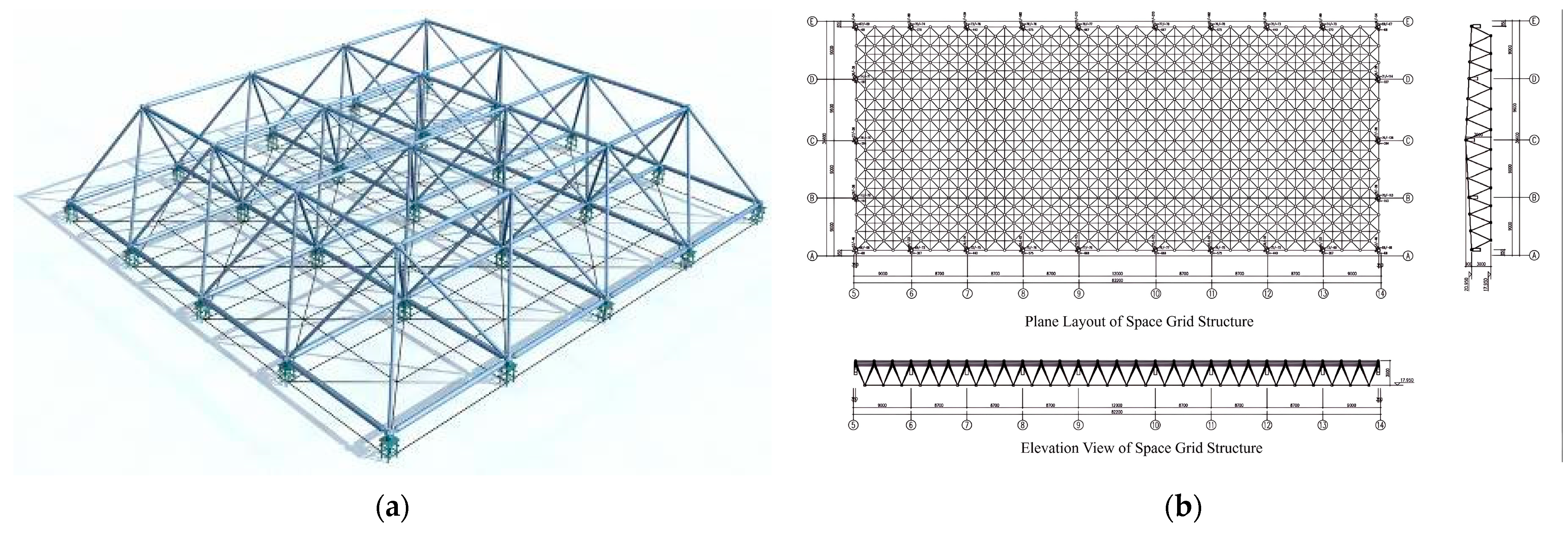
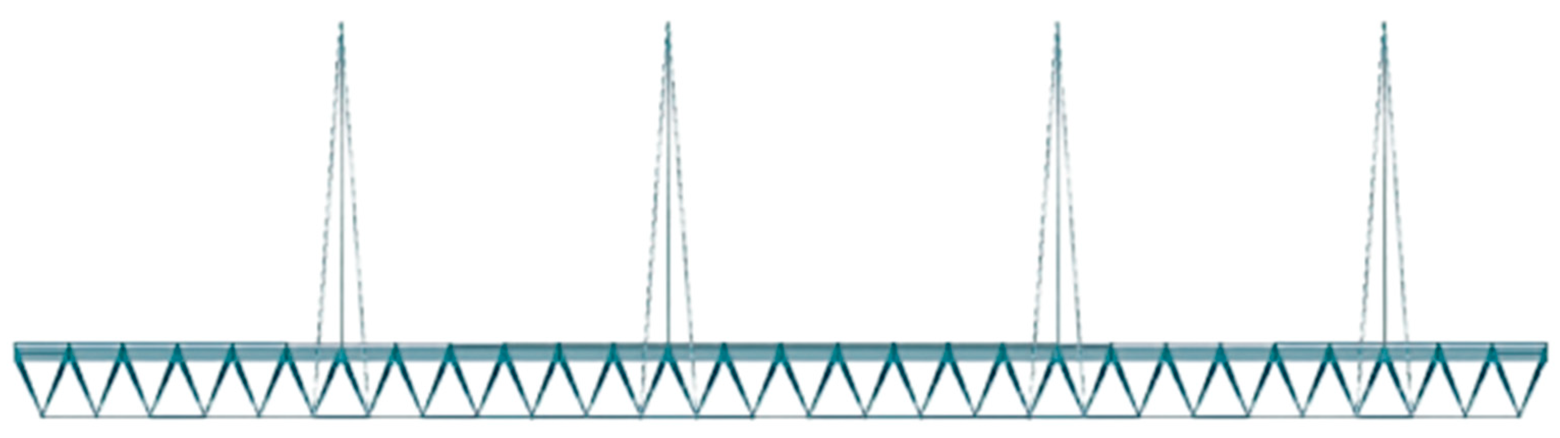
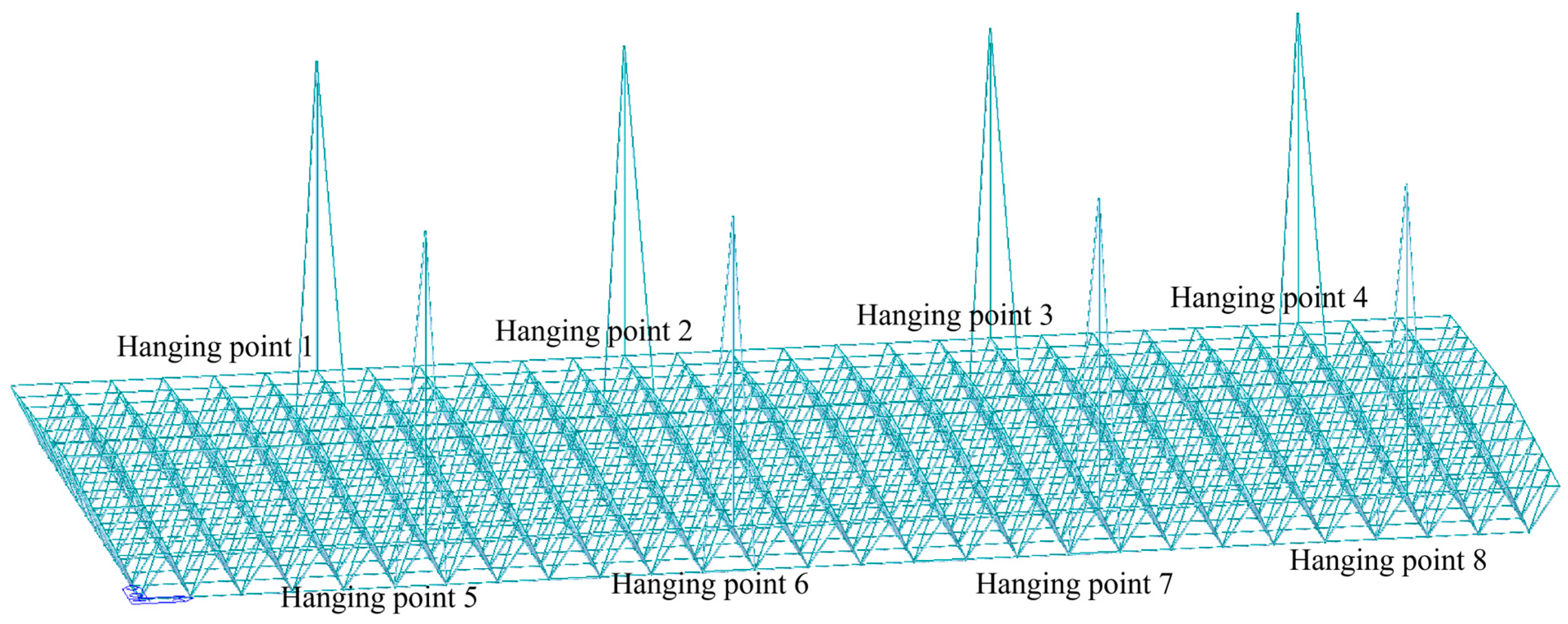
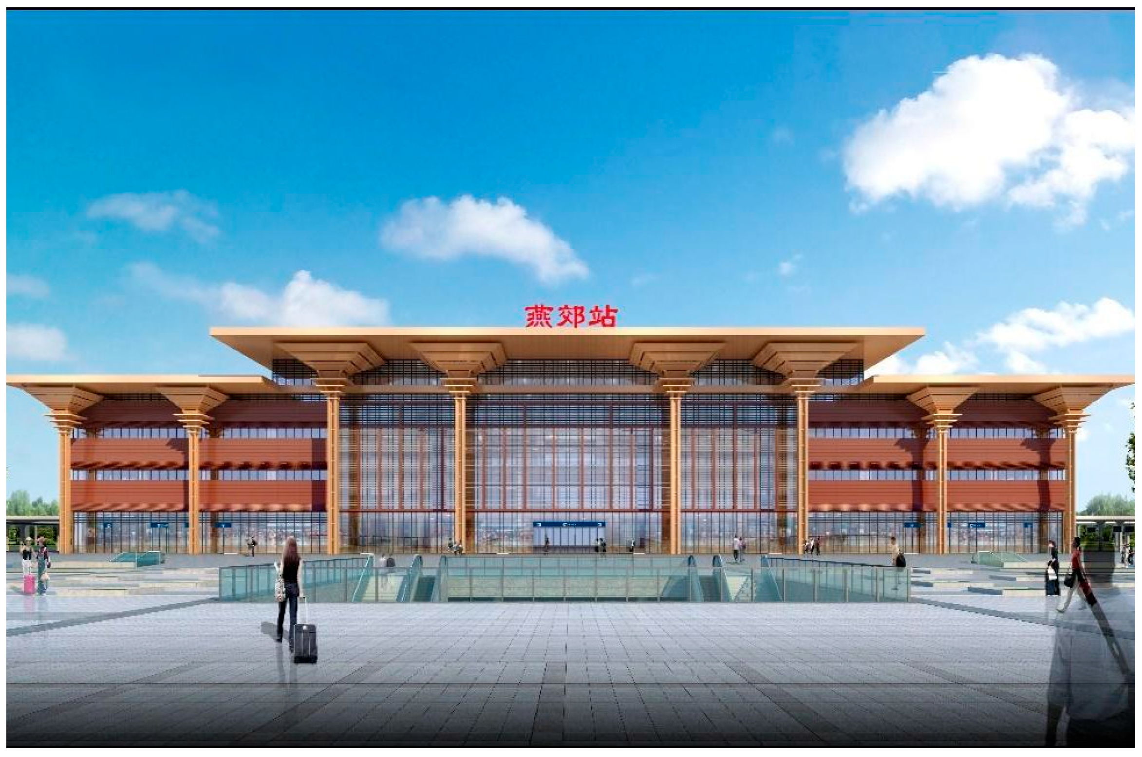
The comprehensive building of Yanjiao station (Figure 1) is an important hub facility of the Beijing–Tangshan intercity railway. The total construction area is 11,982 square meters, and the main structure’s height is 23.0 m. As shown in Figure 2a, the roof system adopts a large-span, orthogonally arranged square pyramid space frame structure equipped with welded spherical joints. According to the architectural blueprints in Figure 2b, the overall planar dimensions of the steel roof are 34.6 m in width (A–E axis) and 82.2 m in length (5–14 axis). The spatial framework consists of localized standard square pyramid units with a characteristic planar mesh size of 3.0 m × 3.0 m and a maximum structural thickness of 3.0 m at the center column lines. The total structural weight of this suspension configuration is approximately 135 tons. The structure is supported by the substructure of the reinforced concrete frame and constructed of Q355 grade steel with a certified thermal conductivity of 48 W/(m·K) (see

Table 1. Thermal properties of the materials [30].

Parameter	Value	Unit
Material	Q355	Steel
Density	7850	kg/m3
Specific Heat Capacity	480	J/(kg·K)
Thermal Conductivity	48	W/(m·K)
Solar Absorptivity α	0.7	-
Coefficient of Linear Expansion	1.2	×10−5/(°C)
Radiation Emissivity ε	0.9	-

for detailed thermodynamic performance). The space frame was constructed using whole hydraulic lifting technology, and a total of eight lifting points are set up. The layout and load distribution of these lifting points show obvious asymmetric characteristics (Figure 3).

These structural characteristics mean that the large-span spatial frame faces severe technical challenges in the construction stage. Firstly, it is very challenging to maintain dynamic balance in the asymmetric lifting system. The deviation between the center of gravity and the center of stiffness leads to overall attitude deflection of the structure. Secondly, because the large-span flexible structure is extremely sensitive to environmental disturbances, how to quantify and compensate for the geometric deformation of vulnerable areas (especially the cantilever end) has become a key technical bottleneck for achieving high-precision construction. In addition, because the lifting operation is carried out in an open environment and the structure is always in a “flexible suspension” state, this also increases the difficulty of construction (Figure 4). The structure shows high sensitivity to external environmental loads. On the one hand, strong solar radiation will produce a complex and non-uniform transient thermal field under the adjustment of the mutual shielding effect of structural components. On the other hand, the coupling effect of high-altitude fluctuating wind fields and thermal fields will dynamically change force distribution inside of the component. Finally, the inherent deviation between the structural center of gravity and the stiffness center further aggravates the complexity of high-precision construction implementation.

Therefore, this study focuses on the flexible suspension stage, aiming to explore the structural mechanical response mechanism under the coupling of the non-uniform thermal field and the variable angle of attack wind field. The purpose is to establish quantitative standards and a theoretical basis for high-precision construction and safety monitoring of large-span asymmetric space frames.

3. Thermal and Wind Field Models Incorporating Geographic and Meteorological Data

3.1. Basic Data and Thermal Properties for Thermal Field Simulation

As for the environmental parameters of thermal field simulation, the construction site is located at 116.83 degrees east longitude, 39.94 degrees north latitude, and 25.5 m above sea level. In order to effectively capture the characteristics and evolution of the thermal field of the structure, a representative date (15 May 2022) during the construction period (13 March 2022 to 6 June 2022) was selected to simulate the 24 h transient thermal field. According to historical meteorological records, the lowest and highest ambient temperatures on this sunny day were 10 °C and 26 °C, respectively. The wind speed is set to a daily average of 2.5 m/s based on meteorological data. It should be noted that wind speed is only used for convective heat transfer calculation in thermal field simulation. In order to study the critical load condition, the subsequent wind load analysis will use the Pufu wind level 6 wind load.

3.2. Transient Solar Radiation Model and Shading Identification Algorithm for Structural Members

3.2.1. Calculation of Solar Geometric Position and Radiation Intensity on Inclined Surfaces

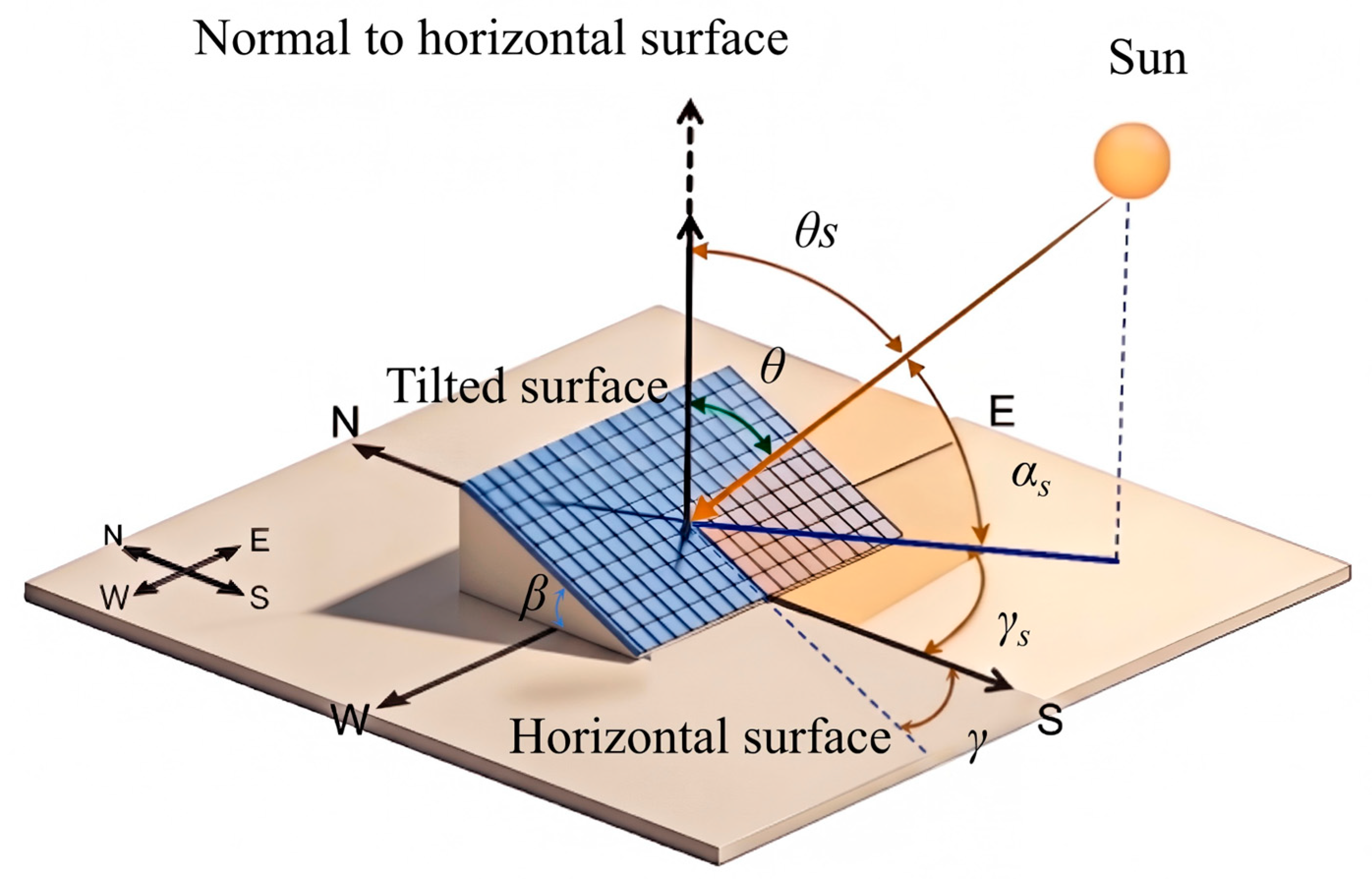
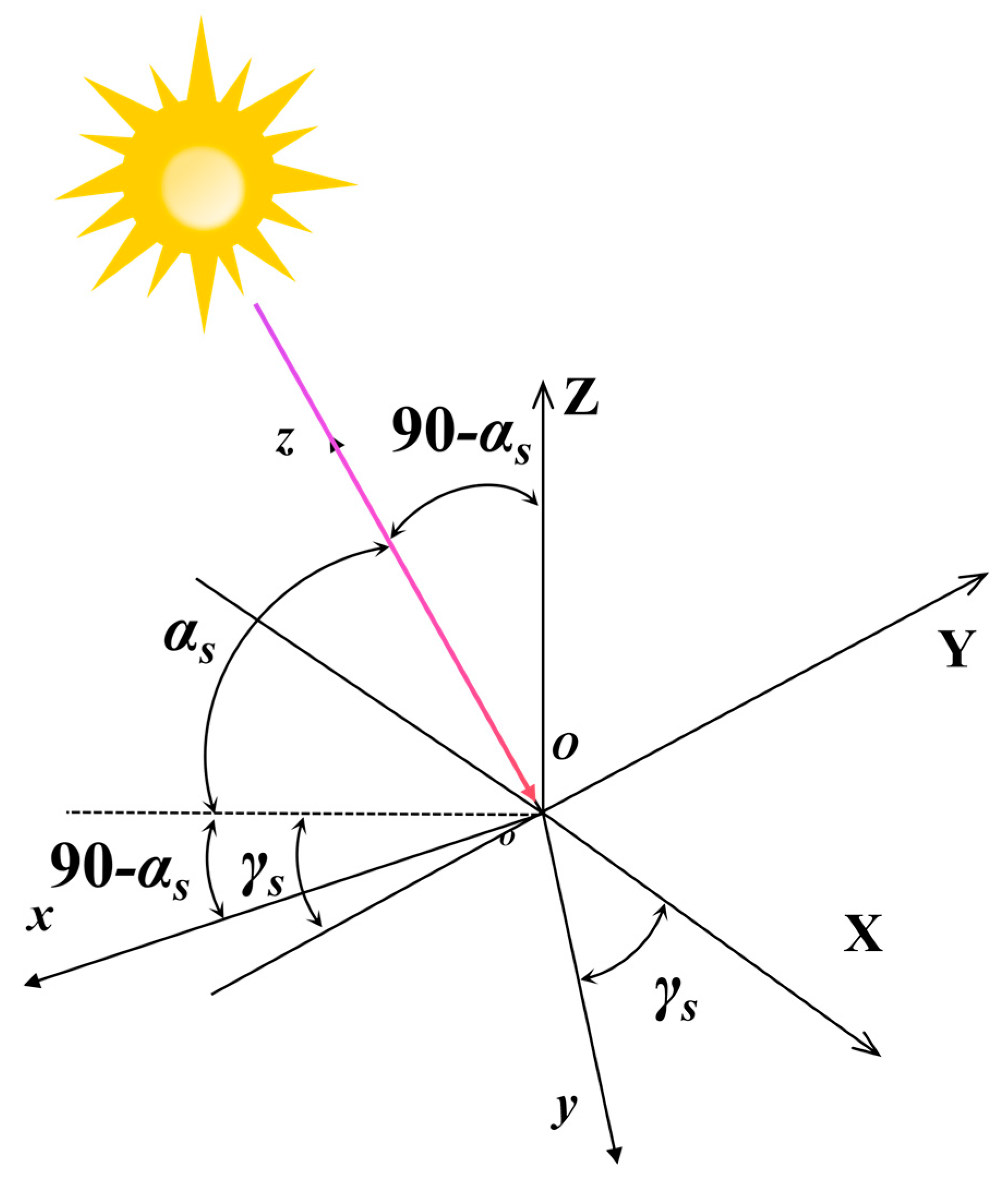
Analyzing the solar thermal response of a structure depends on the precise determination of the solar geometric position at specific spatio-temporal coordinates. This study accounts for the solar declination angle (δ) influenced by the Earth’s revolution, the solar hour angle ($\omega$) driven by rotation, and the specific geographical coordinates of the observation point. Astronomical algorithms were utilized to calculate the solar altitude angle (${\alpha }_s$), azimuth angle (${\gamma }_s$), incidence angle ($\theta$), and tilt angle ($\beta$). This established the transient geometric relationship between solar radiation and the structural surface [32] (Figure 5).

In evaluating radiant energy transmission, this study analyzes the scattering and absorption mechanisms of electromagnetic radiation induced by atmospheric extinction effects. Consequently, the impacts of the Linke turbidity factor [33,34] and atmospheric optical mass [35] on energy attenuation are quantitatively assessed. The total solar radiation received by any terrestrial structural surface comprises three fundamental components: direct radiation, diffuse radiation, and ground-reflected radiation. Accounting for complex atmospheric interactions and the real-time spatial topology of structural members, the solar radiation intensity on an inclined surface under clear sky conditions ($G_T$) is calculated as follows:

$$\begin{array}{rr}{G}_T& = G_b{\displaystyle \frac{\cos \theta }{\sin {\alpha }_s}} + G_d\left({\displaystyle \frac{1 +\cos \beta }{2}}\right)+ (G_b + G_d){\rho }_r\left({\displaystyle \frac{1-\cos \beta }{2}}\right)\end{array}$$

(1)

where ${ G}_b$ and $G_d$ denote the direct and diffuse solar radiation intensities on a horizontal plane, respectively, and ${\rho }_r$ represents the ground reflectance, typically assumed to be 0.2. If $\cos \theta$ is negative (indicating that solar rays cannot directly illuminate the front face of the surface), the contribution of direct radiation is neglected.

3.2.2. Mutual Shading Identification Algorithm for Space Frame Members

Due to the complex spatial topology of long-span steel spatial frames, the dynamic mutual occlusion effect between structural components is the main physical mechanism leading to the formation of a non-uniform thermal field. In order to accurately quantify this phenomenon, this study draws on the hidden surface determination algorithm in image processing and establishes a rigorous recognition process.

• In order to simplify the calculation of the relative spatial position between structural components, the three-dimensional physical space is first mapped to the optical vector coordinate system. In the global coordinate system (OXYZ), the X-axis is defined as pointing east and the Y-axis is facing north. Through a series of coordinate transformations, a local optical coordinate system (oxyz) is introduced in which incident solar radiation propagates along the negative z-axis. The transformation effectively decouples and simplifies the complex three-dimensional shadow calculation problem. As illustrated in Figure 6, the coordinate transformation formula is expressed as follows [36]:

  $$\left[\begin{array}{c}\mathrm{x}\\ \mathrm{y}\\ \mathrm{z}\end{array}\right]=\left[\begin{array}{ccc}\cos (\text{90-}{\alpha }_{\mathrm{s}})& 0& -\sin (\text{90-}{\alpha }_{\mathrm{s}})\\ 0& 1& 0\\ \sin (\text{90-}{\alpha }_{\mathrm{s}})& 0& \cos (\text{90-}{\alpha }_{\mathrm{s}})\end{array}\right]\left[\begin{array}{ccc}\cos (\text{270-}{\gamma }_{\mathrm{s}})& \sin (\text{270-}{\gamma }_{\mathrm{s}})& 0\\ -\sin (\text{270-}{\gamma }_{\mathrm{s}})& \cos (\text{270-}{\gamma }_{\mathrm{s}})& 0\\ 0& 0& 1\end{array}\right]\left[\begin{array}{c}\mathrm{X}\\ \mathrm{Y}\\ \mathrm{Z}\end{array}\right]$$

  (2)

  where ${\gamma }_{\mathrm{s}}$ and ${ \alpha }_{\mathrm{s}}$ denote the solar azimuth angle and the solar altitude angle at any arbitrary instant, respectively.
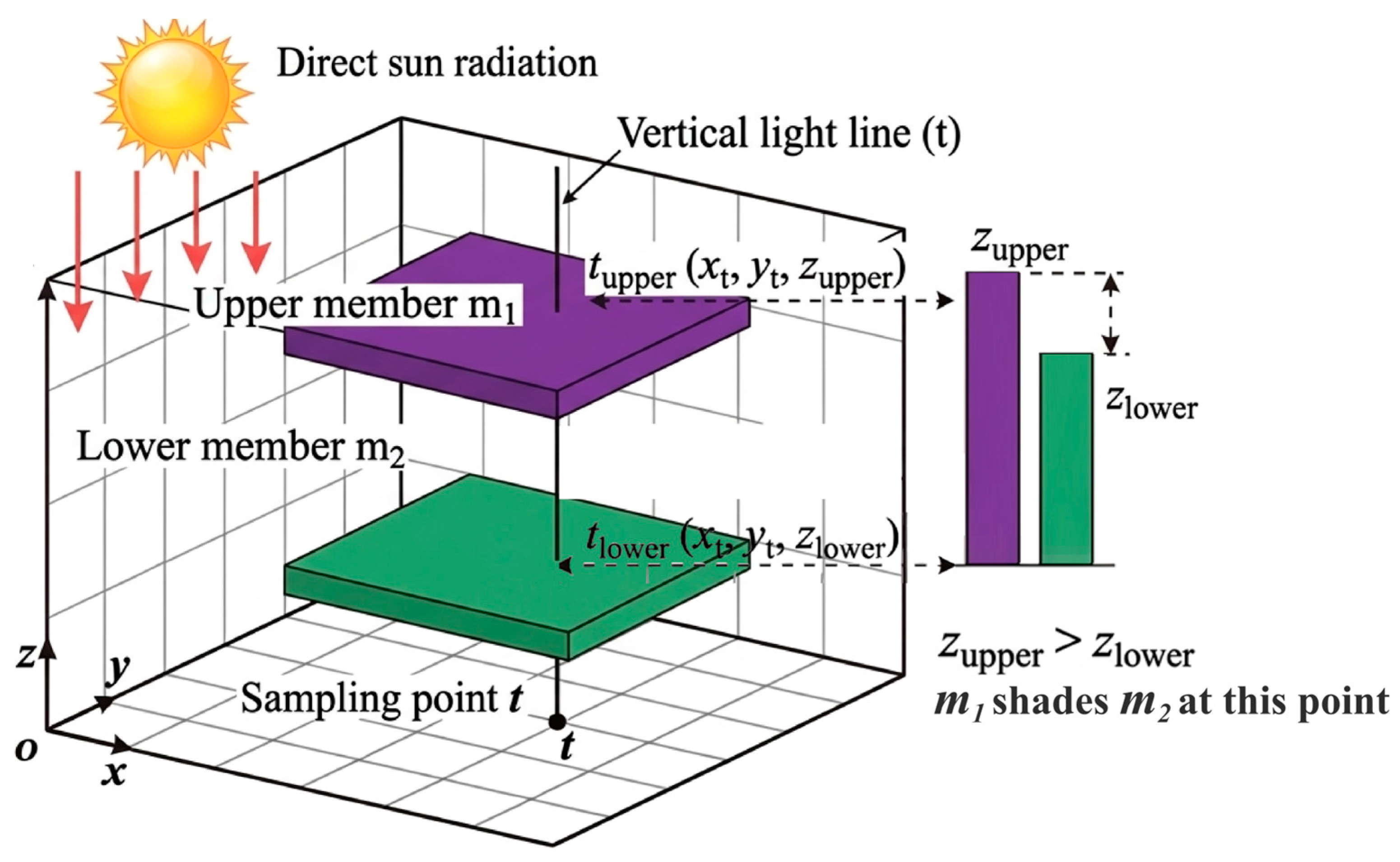
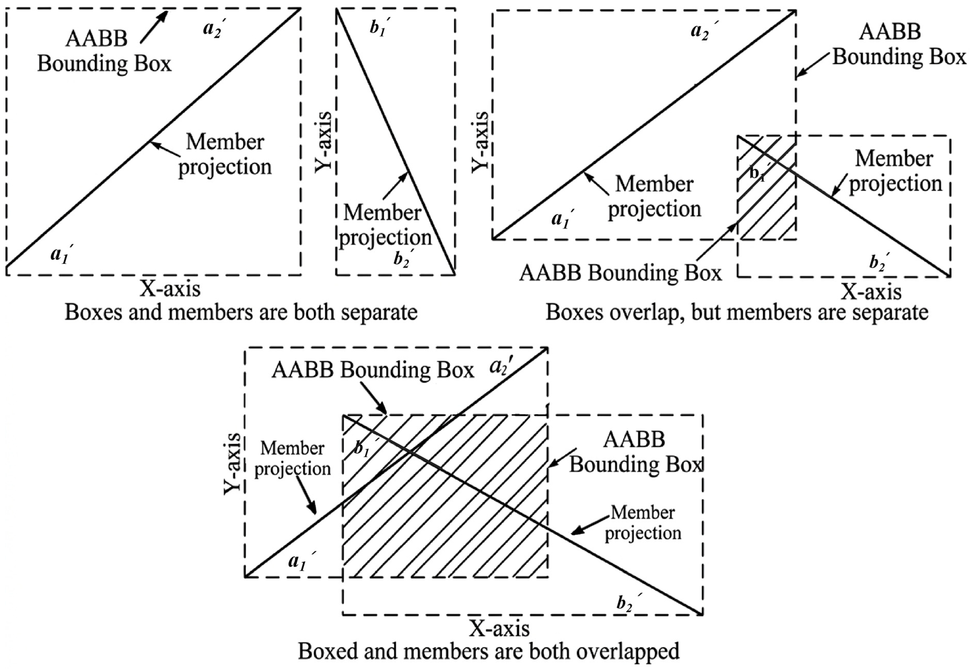
• To balance computational accuracy and efficiency for complex structural systems, this study introduces a pre-detection algorithm based on Axis-Aligned Bounding Boxes (AABB). The algorithm first constructs a minimum bounding box for each member based on its projection onto the xoy plane of the light vector coordinate system (Figure 7). If the bounding boxes of two members do not overlap, subsequent refined calculations are bypassed. For members that pass this initial screening, depth information (z-axis coordinates) is incorporated. By comparing the relative positions of structural members along the light propagation direction, the shading hierarchy is established (Figure 8), thereby identifying the shading source and the shaded members.
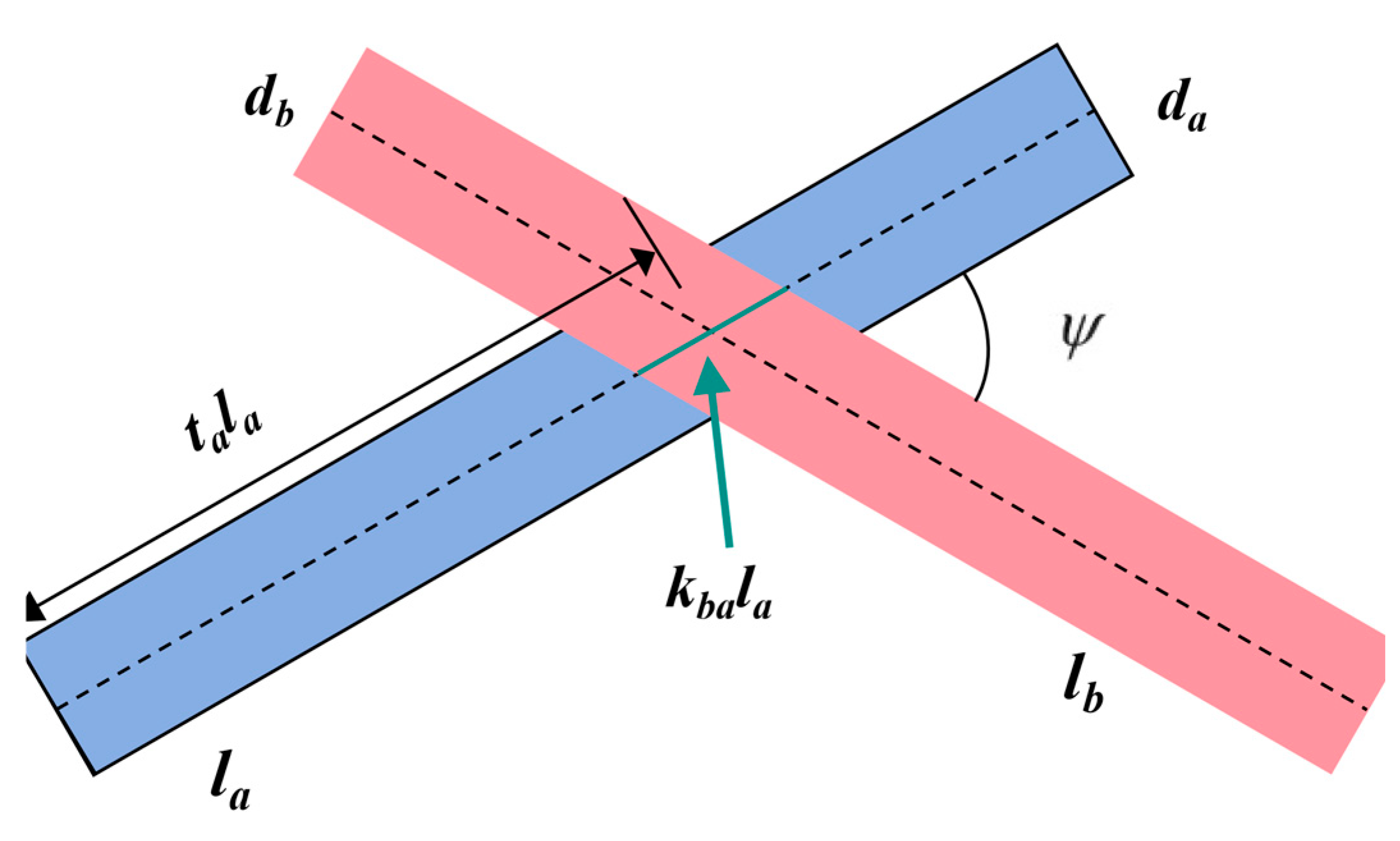
• Once the shading relationships are established, the shadow interval distribution on the surface of the shaded member is precisely calculated based on the member’s cross-sectional diameter and the angle between its axes (Figure 9). To eliminate geometric redundancy resulting from multiple overlapping shading, this study performs Boolean union operations on the stored shadow intervals to extract the net shadow distribution sequence. Accordingly, the solar direct radiation coefficient ($r_{si}$) is defined to quantitatively characterize the attenuation of direct solar radiation energy induced by shading effects, which is obtained as follows:

  $$r_{\mathit{si}} = 1-\sum _j{k}_{\mathit{ji}}^{\prime }$$

  (3)

  where $k_{\mathit{ji}}^{\prime }$ represents the normalized length of non-overlapping shadow intervals cast by the shading member j onto the shaded member i. This coefficient provides an objective measure of the proportion of direct solar energy effectively intercepted by member i, thereby serving as a quantitative basis for subsequent non-uniform thermal response assessments of the affected structure.

3.2.3. Calculation of Total Solar Radiation Absorption by Members Considering Shading Effects

Traditional models often fail to accurately describe the complex thermal state of circular tubular members widely used in large-span spatial steel structures. Based on the research framework established by the research framework established [9], this study developed an energy capture model that can explicitly consider the shading effect. This model breaks through the simplified method of characterizing the overall thermal state only by the axis inclination angle. By using micro-element calculation technology, the surface of the circular tube is discretized into a series of longitudinal micro-element strips, and then these micro-element regions and their dynamic incident angles are circumferentially integrated to accurately quantify the total radiation energy captured by the component in the unit time interval. For diffuse radiation and ground reflection radiation, the energy gain is highly sensitive to the real-time incident angle of the receiving surface. In this study, the circumferential energy weighted integral strategy is used to aggregate the non-uniformly distributed radiation components so as to accurately characterize the overall radiation intensity of the tubular component. For the direct radiation component, the effective projection area of the component based on the optical vector coordinate system is calculated. By incorporating the solar direct radiation coefficient ($r_{si}$) previously defined, the modified direct radiation gain ($I_b$)—accounting for energy attenuation due to shading effects—is obtained as follows:

$$I_b = r_{\mathit{si}} l’d{G}_b{\displaystyle \frac{1}{\mathit{sin}{\alpha }_s}}$$

(4)

where $l’$ denotes the effective projected length of the member axis and $d$ represents the outer diameter of the circular cross-section.

Accounting for the spectral characteristics of the member’s outer surface, this study incorporates solar absorptivity ($\alpha$) to quantify energy conversion efficiency. Consequently, the total solar radiant energy captured by the tubular member within a unit time interval can be expressed as

$$I=\alpha (I_b+I_d+I_r)$$

(5)

where the solar absorptivity ($\alpha$) is primarily determined by the material properties and coating characteristics of the member’s surface. $I_b, I_d$, and $I_r$ denote the direct, diffuse, and ground-reflected solar radiation components received by the member per unit time, respectively. The solar absorptivity (α) is determined based on the values provided in Table 1.

3.3. Theory of Surface Heat Exchange Boundary Conditions for the Space Frame

3.3.1. Convective Heat Transfer Model

Due to the continuous movement of the surrounding air, the surface of the structure will continue to carry out convective heat exchange with the surrounding air. This process essentially follows Newton’s cooling law, which is expressed as follows:

$$q = \overline{h}(T_a-T_b)$$

(6)

where $\overline{h}$ denotes the convective heat transfer coefficient of the structural surface and $T_a$ and $T_b$ represent the ambient air temperature and the real-time surface temperature of the member, respectively.

For the circular tubular members prevalent in the large-span steel space frames investigated herein, the surface convective heat transfer coefficient ($\overline{h}$) is governed by physical parameters including airflow velocity, kinematic viscosity, and the Reynolds number. Referring to the classical heat transfer model for flow over a single cylinder detailed in [37], this study introduces Reynolds-number-dependent empirical coefficients to achieve dynamic correction of convective heat transfer intensity under varying wind speed conditions.

3.3.2. Long-Wave Radiation Exchange Mechanism Among Members

The thermal radiation exchange between an object and its surrounding environment is continuous, which is called long-wave radiation exchange. The surrounding environment can be idealized as a blackbody with the same temperature as the ambient air, and the visual direction factor relative to the object is 1. According to the Stefan–Boltzmann law of blackbody radiation, the heat flux density of long-wave radiation exchange between the object and the environment can be expressed as

$$q=\epsilon \sigma (T^{ 4}-T_s^{ 4})$$

(7)

where ε denotes the radiation emissivity of the structural surface, determined from Table 1 based on material and surface properties; $\sigma$ represents the Stefan–Boltzmann constant, taken as 5.67 × 10⁻⁸ W/(m²·K⁴); $T$ denotes the absolute temperature of the structural member; and $T_s$ denotes the absolute temperature of the surrounding environment.

3.4. Numerical Simulation of Non-Uniform Thermal and Wind Fields During the Lifting Phase

3.4.1. FEA-Based Calculation Module for Non-Uniform Transient Thermal Fields

This study introduces the transient thermal field analysis method based on the finite element method (FEM) of heat conduction. In the Cartesian coordinate system, the transient heat conduction process in the space frame is described by the differential equation derived from the law of conservation of energy and the Fourier heat conduction law. By introducing three thermodynamic boundary conditions and spatial discretization of the continuous medium, the transient heat conduction problem is re-expressed as a finite element matrix equation based on the integral weak form. In order to accurately capture the transient response of the structure over time, this study adopts the standard numerical calculation method widely recognized in engineering practice [38]:

$$[C \left]\right\{{\dot{T}}_e(t\left)\right\} + \left(\left[K^{ d}\right] + \left[K^{ c}\right]\right)\left\{T_e\right(t\left)\right\} = \{Q^{ f} \}+ \{Q^{ c} \} +\{Q^{ g} \}$$

(8)

where $\left[C\right]$ denotes the heat capacity matrix; $\left[K^d\right]$ represents the heat conduction matrix; and $\left[K^c\right]$ stands for the convective heat transfer matrix. $\left\{T_e\right(t\left)\right\}$ is the nodal temperature vector, and $\{{\dot{T}}_e(t\left)\right\}$ represents its time derivative. Regarding the load vectors, $\left\{Q^{ f}\right\}$ is defined as the heat flux vector; $\left\{Q^{ c}\right\}$ represents the convective heat flow vector; and $\left\{Q^{ g}\right\}$ denotes the internal heat generation vector. This equation is essentially a system of first-order ordinary differential equations with respect to time. Given the dynamic, time-varying nature of the boundary conditions under solar irradiation, numerical time-stepping integration is mandatory to capture the transient thermal response of the structure over time.

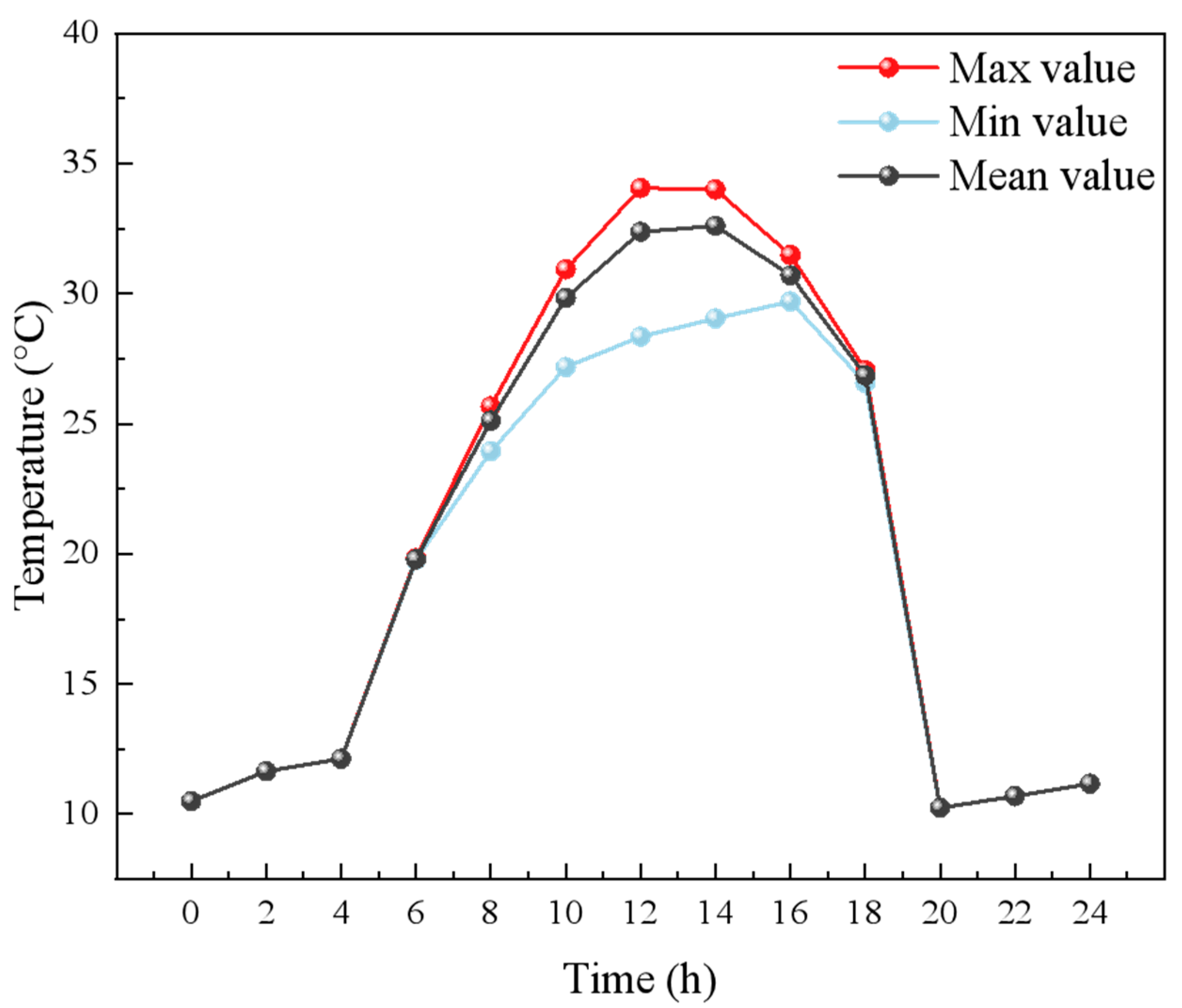
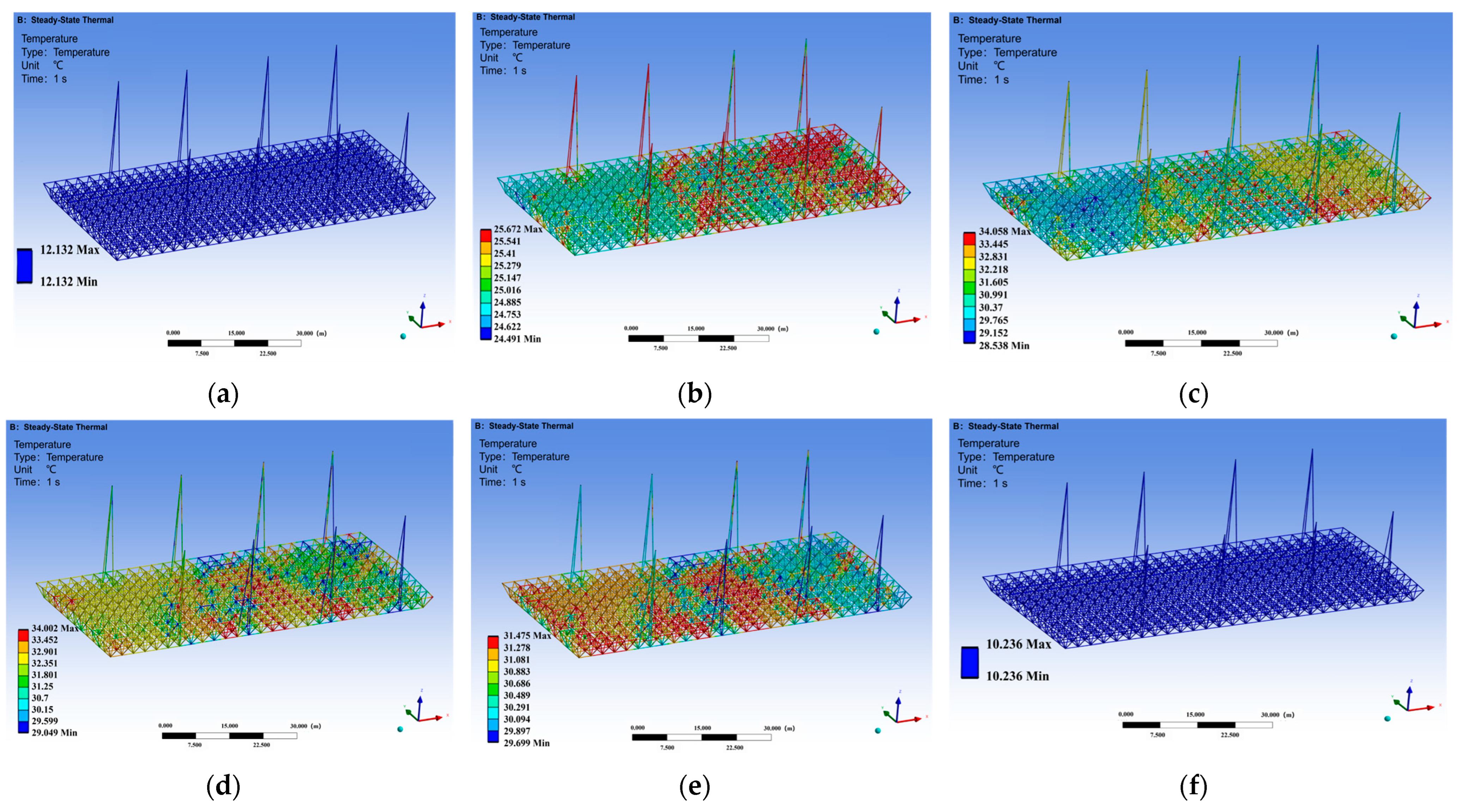
Based on the above thermodynamic analysis framework and numerical discretization strategy, this study successfully obtained the non-uniform transient thermal field data set of the target model under complex solar radiation conditions. The variation trend of the temperature of each component with time is shown in Figure 10, where “maximum”, “minimum”, and “average” represent the highest, lowest, and average temperatures of all 2711 structural components at each time step, respectively. The change in structural temperature is mainly driven by the synergistic effect of solar radiation intensity and ambient air temperature fluctuation. In view of its significant diurnal variation characteristics, the structural temperature shows a clear time correlation in the 24 h cycle. Although the variation trend of the maximum temperature of the structure is consistent with the ambient air temperature, it shows significant nonlinear characteristics. The specific evolution characteristics are as follows.

The temperature field of the space frame shows significant transient evolution characteristics and spatio-temporal inhomogeneity. During the early morning period (0:00–6:00), long-wave radiation cooling is dominant, the structure reaches a thermal equilibrium state, and the temperature approaches the daily minimum (about 10–12 °C). After sunrise, the solar radiation increases, triggering a rapid warming phase, and the upper chord temperature reaches a peak at 12:00 (about 34 °C). The sharp temperature rise observed from 8:00 to 10:00 highlights the high sensitivity of steel structures to solar radiation. It is worth noting that under the combined action of thermal inertia and convective heat transfer efficiency, the average temperature of the structure reaches a peak at about 14:00, which is about 3 h later than the radiation peak. After sunset, the structure undergoes a cooling process driven by thermal gradient that is fast at the beginning and then gradually slows down. As the temperature gradient dissipates, the temperature distribution changes from warm to cold, thus completing a complete thermal cycle before sunrise. Figure 11 shows the temperature field distribution of the structural members under the representative time step, in which 4 h and 20 h correspond to the situation before sunrise and after sunset, respectively, and there is no direct solar radiation at this time.

3.4.2. Variable Angle-of-Attack Wind Field Calculation Model Based on Standard Formulas

This study primarily investigates the impact of varying wind attack angles on the mechanical response of a large-span steel truss during asymmetric lifting. Consequently, the wind pressure model for numerical simulations was established using the automated wind load generation module in Midas Gen (2021, MIDAS Information Technology Co., Ltd., Seongnam, Republic of Korea), in strict accordance with the Load Code for the Design of Building Structures (GB 50009-2012) [39]. By presetting key parameters such as basic wind pressure ($w_{0 }$), ground roughness category, and structural damping ratio, the software automatically determined the height-dependent wind pressure coefficient (${ \mu }_{z }$) and the wind vibration coefficient (${ \beta }_z)$. For the circular tubular members in the support system, the shape coefficient (${\mu }_s$) and the wind-blocking coefficient (Φ) were precisely defined, transforming the complex spatial random wind field into equivalent static loads ($w_k)$ applied to structural nodes or elements, thereby achieving precise coupling between wind loads and solar thermal effects in both time and space.

The along-wind pressure is calculated in accordance with the Load Code for the Design of Building Structures (GB 50009-2012) [39]:

$$w_k = {\beta }_z{\mu }_s{\mu }_z{w}_0$$

(9)

• ${\beta }_z:$ Wind-Induced Vibration Coefficient;
• ${\mu }_s$: Wind load shape coefficient. In determining ${\mu }_s$, the spatial shading effects among structural members are comprehensively considered. Based on GB 50009-2012 and empirical parameters (i.e., wind-blocking coefficient Φ ≈ 0.2 and spacing ratio $s/h \approx 1.0$), a shading reduction factor of $\eta$ = 0.8 is adopted. By compounding the base shape coefficient of the windward member (${\mu }_{s0}$ = 1.2) with the shading factor, wind pressure attenuation on trailing members is rigorously corrected. This yields a final shape coefficient of ${\mu }_s$ = 0.96, ensuring physical consistency between boundary conditions and wind pressure distribution in the non-uniform thermal field analysis;
• ${\beta }_z$: Wind pressure height variation coefficient;
• ${ w}_0$: Basic wind pressure. As structural lifting is suspended when wind speeds exceed Grade 6, ${ w}_0$ is set to 0.12 kN/m², corresponding to the Grade 6 wind load threshold.

4. Finite Element Modeling and Dual-Platform Verification

4.1. Configuration of Modeling Parameters

The primary structural members are modeled using Q355 steel, with the constitutive relationship simplified as an isotropic, ideal elastic–plastic model governed by the von Mises yield criterion. To facilitate subsequent dynamic response analyses, the specific physical parameters and cross-sectional properties of the members are detailed in

Table 2. Physical properties of Q355 steel used in the finite element model.

Parameter	Value	Unit
Modulus of elasticity E	2.06 × 105	MPa
Poisson’s ratio ν	0.3	-
SUnit weight γ	78.5	kN/m3
Coefficient of linear expansion α	1.2 × 10−5	/°C
Thermal conductivity	48	W/(m·K)
Damping ratio	0.02	-

and

Table 3. Cross-sectional properties of tubular members.

Member Designation	Outer Diameter/(m)	Wall Thickness/(m)
P 60 × 3.5	0.0600	0.00350
P 75.5 × 3.75	0.0755	0.00375
P 88.5 × 4	0.0885	0.00400
P 114 × 4	0.1140	0.00400
P 140 × 4	0.1400	0.00400
P 159 × 6	0.1590	0.00600

, respectively.

4.2. Finite Element Modeling

In this study, Midas Gen software (2021, Midas Information Technology Co., Ltd., Seongnam, Republic of Korea) was used to establish a refined finite element model of the spatial frame of Yanjiao station in the flexible suspension stage. In order to facilitate the direct application of surface wind pressure, the space beam element is adopted. The rotational degrees of freedom are released at the non-critical internal nodes to ensure that the structure is in an articulated assembly state, thereby eliminating the artificial bending moment at the continuous nodes and accurately simulating the behavior characteristics of the spatial frame members dominated by the axial force. The boundary conditions of the lifting point are defined by constraining the vertical displacement while allowing horizontal translation to capture swing behavior during the hydraulic lifting process. The model introduces geometric nonlinearity to consider the contribution of large displacement stiffness. In terms of load conditions, the dead load is accurately calculated by the dead weight of the structure and the added mass of the joint ball; based on the solar radiation model of Matlab (R2024b, MathWorks, Natick, MA, USA) the non-uniform thermal field is generated and applied as the unit temperature load. The fluctuating wind load is converted into the equivalent static load by the wind pressure function and the wind vibration coefficient of the beam element. The Newton–Raphson iteration method is used to solve the problem, and the convergence is controlled by the energy criterion (ϵ ≤ 10⁻⁴) to ensure the calculation accuracy of large displacement nonlinearity and plastic energy dissipation analysis.

4.3. Dual-Platform Verification

After completing the preliminary development of the spatial frame finite element (FE) model of Yanjiao Station, the research team adopted a “two-platform benchmark” strategy to eliminate systematic deviations that may be introduced by specific platform algorithms or modeling methods. By comparing the calculation results of the general finite element software Ansys (2024 R2, Ansys Inc., Canonsburg, PA, USA) with the results of the engineering software Midas Gen, the reliability of the mechanical response data obtained from the benchmark test is verified.

In order to ensure strict “isomorphism verification”, the mechanical parameters of the two simulation platforms are strictly unified. Specifically, a unified space truss element is used. Link element is used in Ansys, and Truss element is used in Midas Gen; both models only retain the axial stiffness to eliminate the bending effect. In addition, the geometric parameters of the circular hollow section are standardized to P 88.5 × 4 specifications, and all structural members are made of Q355 steel. In terms of loading conditions, only the structural weight (g = 9.8 m/s²) is applied to evaluate the mass integration capability of the two platforms when dealing with large-scale matrices. Finally, in terms of boundary conditions, the lifting point adopts general support, while the connection point between the steel strand and the truss structure adopts fixed support.

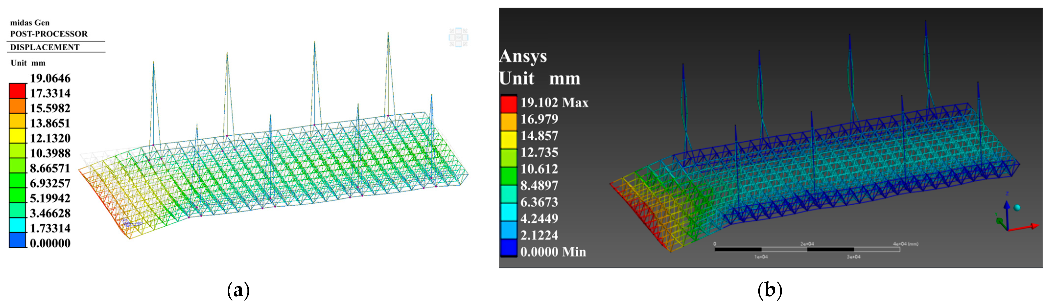
As illustrated in Figure 12, the displacement field distributions generated by both platforms exhibit excellent correspondence, with the space frame demonstrating minimal deflection in the center and progressively increasing deflection toward the cantilevered ends and peripheral regions. Both models captured the maximum deflection at the left cantilevered edge, with the color gradients evolving in a fully consistent and monotonic manner. This provides intuitive validation of the spatial topological consistency in the assembly of mass and stiffness matrices, thereby ensuring numerical accuracy. A quantitative error analysis was conducted by extracting key data points from the displacement contours; the maximum vertical displacement calculated by Midas Gen was 19.064 mm, compared to 19.102 mm obtained from Ansys. This yields a relative error of 0.2%, calculated as Error = (19.102 − 19.064)/19.102 × 100% = 0.2%.

Quantitative benchmark tests show that the relative error between the two independent solvers is only 0.2% when dealing with large-scale spatial frames (721 nodes and 2711 units), which is much lower than the reliability threshold of 5%. This difference is due to the small cumulative error inherent in the numerical truncation and unit conversion algorithms of the dual-precision Ansys solver and the engineering-oriented Midas Gen solver. Cross-platform verification confirms that the basic static displacement response is highly consistent, and the relative error is only 0.2%, which fully meets the engineering reliability requirements. These research results verify the accuracy of the model in terms of geometric topology, material constitutive characteristics, and load mapping and establish a reliable numerical benchmark for the subsequent multi-field coupling nonlinear response analysis.

4.4. Comparison with Field-Measured Data and FE Model Validation

4.4.1. Field Monitoring Scheme for Lifting Forces

The integral hydraulic synchronous lifting of large-span space frame structures represents a risk-sensitive transient construction process, where the floating framework is extraordinarily susceptible to multi-field synergistic disturbances and non-uniform thermal strains. To comprehensively validate the feasibility of the previously established multi-field coupled geometric nonlinear finite element analytical framework, field empirical measurement data are introduced in this section to execute rigorous mechanical verification.

The total dead weight of the orthogonally arranged square pyramid space frame at Yanjiao Station is approximately 135 tons, translating into a baseline global static lifting force requirement of roughly 1323 kN. Due to the asymmetric spatial configuration and non-uniform load distribution of the eight hydraulic hoisting points, a marked eccentric amplification effect between the center of mass and the center of stiffness is natively generated within the flexible suspension system. Throughout the vertical lifting progression, high-precision pressure transducers integrated into the hydraulic manifolds of the hoisting jack clusters were utilized to sample the active telemetry of the real-time lifting forces. In this section, the telemetry from Lifting Point 1 (Hanging Point 1), which governs the structural stability margins of the adjacent weak cantilever peripheries and undergoes the most complex translational-torsional coupling effects, is designated as the primary validation baseline. The empirical force datasets were continuously logged across the complete vertical displacement from 0 to 45 m.

4.4.2. Comparative Analysis and Quantitative Error Verification of Lifting Forces

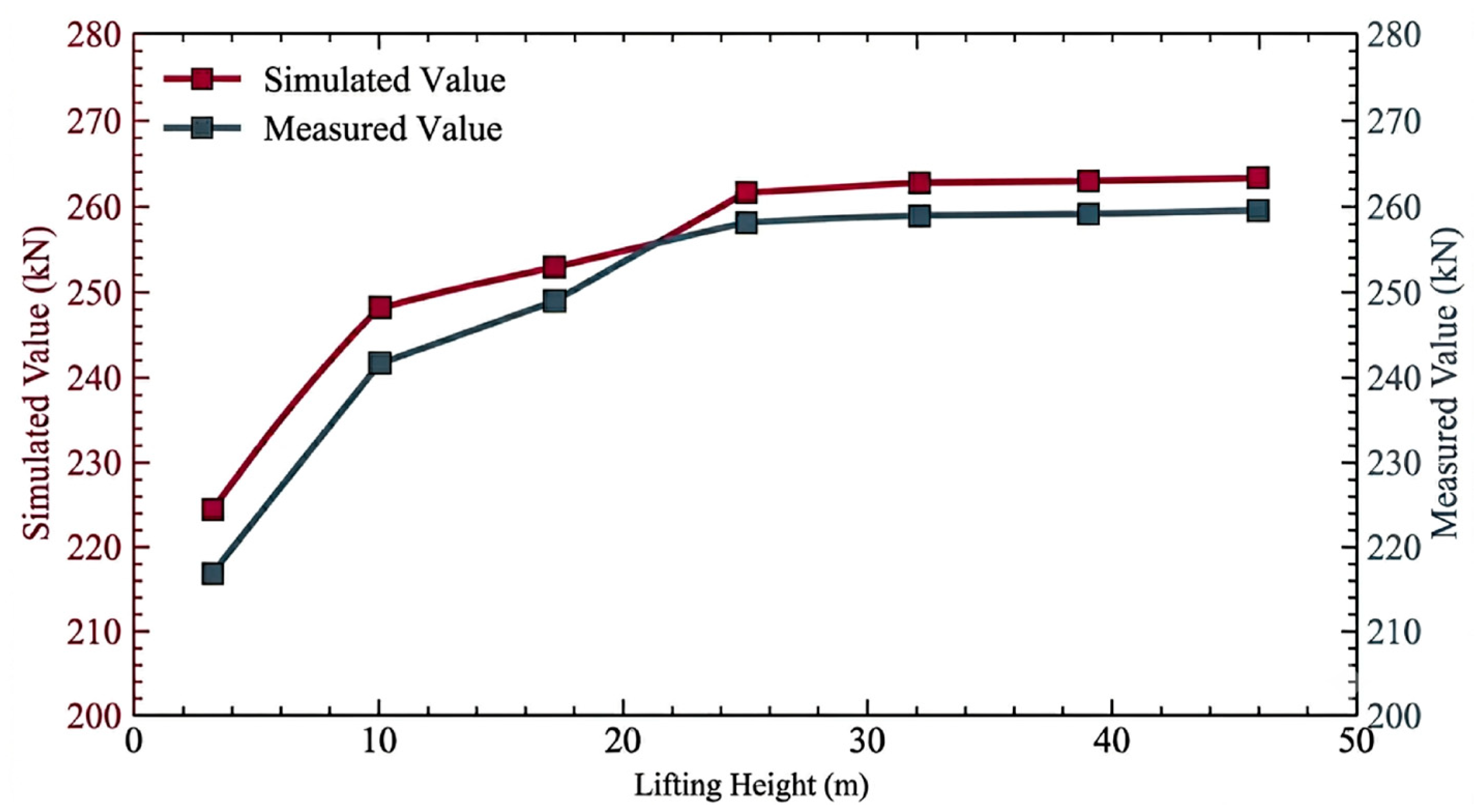
According to the active field telemetry retrieved from the data loggers and the discrete solvers computed by the finite element platform, Figure 13 illustrates the comparative profiles of the dynamic lifting force at Lifting Point 1 as a function of the lifting height. To quantitatively judge the mathematical completeness of the simulation model, discrete datasets at representative lifting elevations are extracted for rigorous error evaluation, as tabulated in

Table 4. Quantitative comparison between simulated and measured lifting forces at Lifting Point 1.

Height/m	Simulated Value/kN	Measured Value/kN	Absolute Error/kN	Relative Error/%
3.0	224.50	216.80	+7.70	+3.43%
10.0	248.60	242.10	+3.50	+1.41%
17.0	253.15	249.20	+3.95	+1.56%
25.0	258.40	262.10	−3.70	−1.43%
32.0	259.10	263.20	−4.10	−1.58%
38.0	259.25	263.50	−4.25	−1.64%

.

Superimposing the finite element numerical curves against the empirical telemetry datasets from Figure 13 and Table 4 demonstrates exceptional dynamic convergence. During the initial launch phase (0–10 m), the model precisely captures the nonlinear climbing trajectory induced by boundary transformations and automatic alignment corrections. In the high-altitude steady segment (25–45 m), the measured dataset marginally overshoots the idealized static baseline (fluctuating tightly within a minor −1.43% to −1.66% relative error domain); this elegant discrepancy faithfully reflects the second-order amplification and translation–torsion micro-oscillations driven by the atmospheric wind field, emphasizing the practical realism of the simulation. Quantitatively, the global peak relative error across the entire tracking profile is rigorously constrained below 3.43%, sitting well within the conservative 5% structural engineering validation threshold. This high-fidelity agreement conclusively certifies the superior mathematical accuracy and complete reliability of the developed simulation framework regarding structural mesh topology, material constitutiveness, and multi-field boundary definitions.

5. Mechanical Response Analysis and Critical Load Case Identification of the Space Frame Under Individual Environmental Loads

5.1. Mechanical Performance and Critical Load Case Analysis Under Non-Uniform Thermal Fields

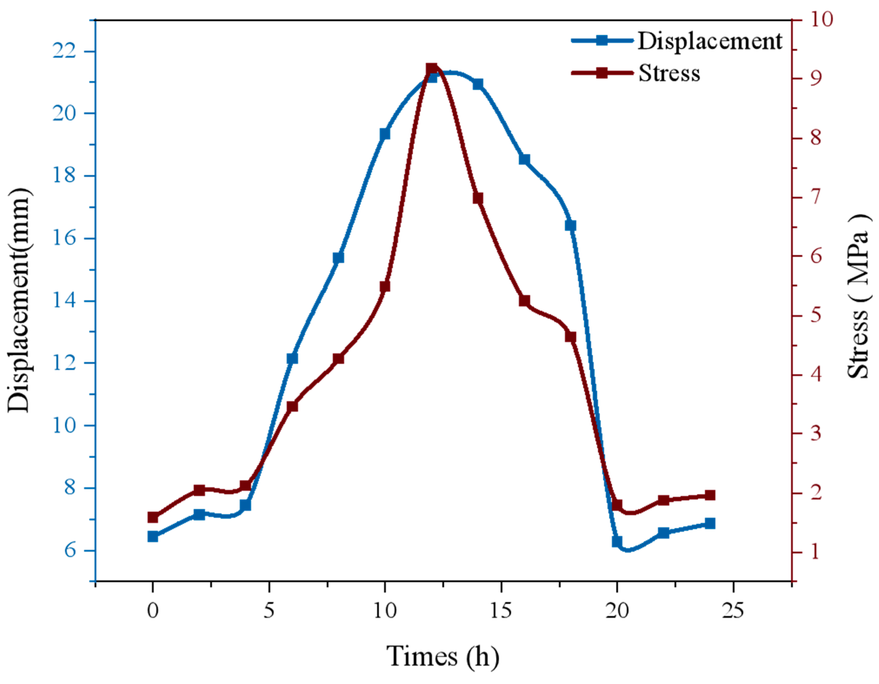
Based on the previously developed and cross-validated optimized finite element model on the dual platform, this section uses the digital solar thermal field as the time-varying boundary driving source to conduct a comprehensive numerical simulation of the thermodynamic response of the Yanjiao station space frame in a continuous 24 h period. The time series relationship between displacement, stress, and non-uniform thermal field is shown in Figure 14, and the corresponding contour map is attached (Figure 15) Through in-depth analysis of displacement evolution curves and stress time history data, this study aims to quantitatively reveal how ambient temperature fluctuations affect the overall stability of space frames under flexible suspension. These research results provide a scientific basis for precise control and structural health monitoring during asymmetric lifting.

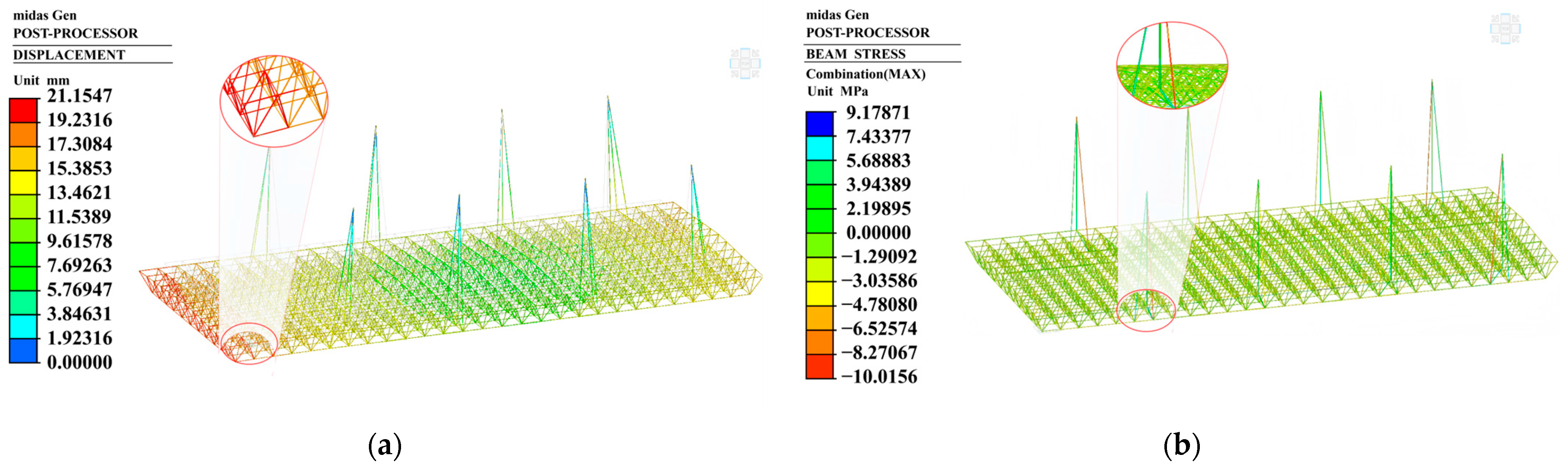
Numerical simulations over a continuous 24 h cycle demonstrate that both displacement and stress responses exhibit a distinct unimodal evolution pattern synchronized with solar radiation, peaking at 12:00. At this instant, the maximum displacement reaches 21.15 mm (Figure 15a), representing a 160% increase compared to the baseline at 0:00, which is free from solar radiation, while the maximum stress peaks at 9.18 MPa (Figure 15b). These extreme values are concentrated in the cantilever edge area exposed to sunlight, showing significant spatial asymmetry. This phenomenon is mainly due to the vertical constraints at the lifting point of the flexible suspension platform; these constraints limit the free thermal expansion of the material, thereby converting the thermal strain into a significant residual thermal stress. At the same time, the non-uniform thermal field generated by the shading effect of the component destroys the geometric equilibrium state, resulting in the redistribution of internal forces and amplifying the second-order displacement effect. In general, there is a high spatial–temporal correlation between the thermal response of the spatial frame and solar radiation. Due to the asymmetry of topological structure and shading effect, the system shows obvious spatial heterogeneity. As the key period of structural deformation, the secondary internal force and displacement offset usually occur at about 12:00 noon, which poses a major threat to construction accuracy.

5.2. Mechanical Performance and Critical Load Case Analysis Under Wind Fields

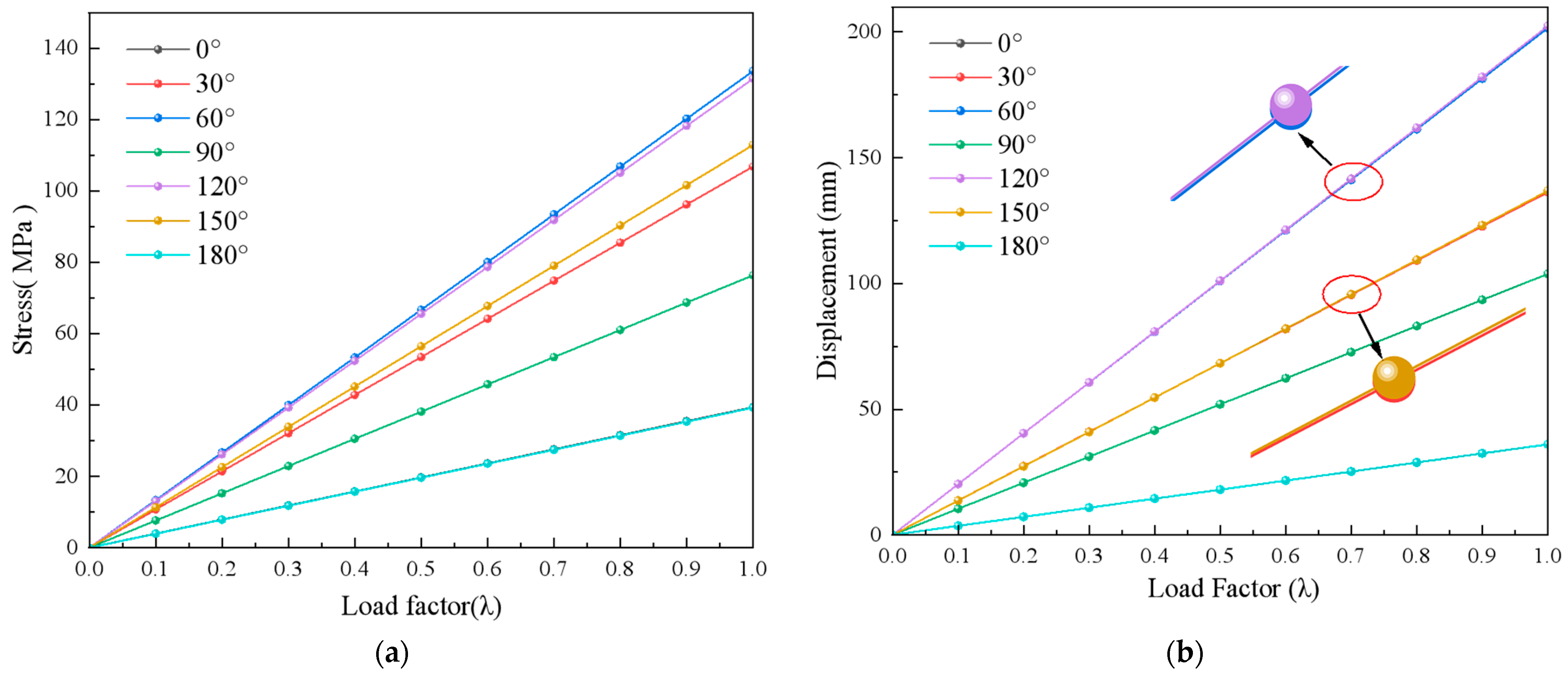
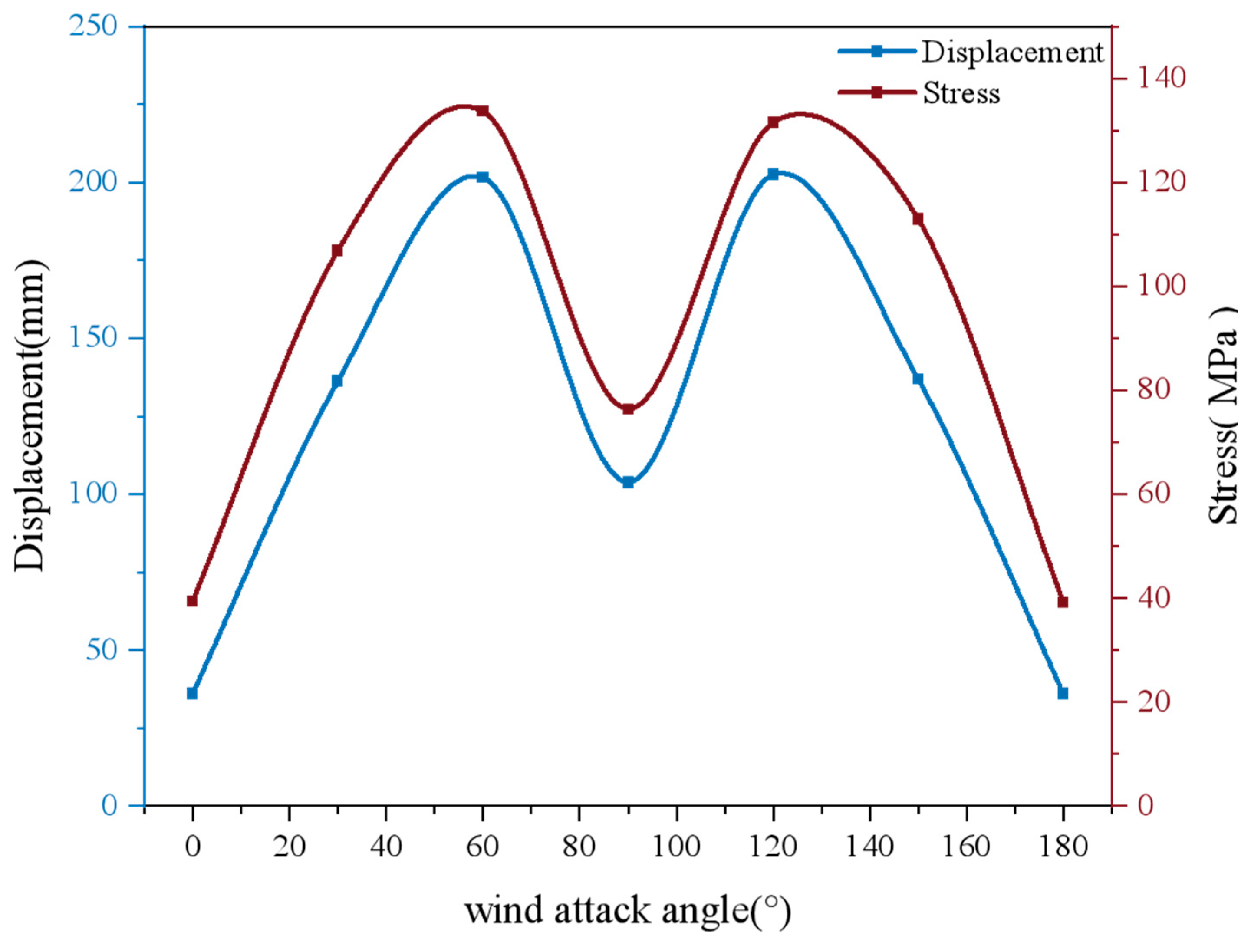
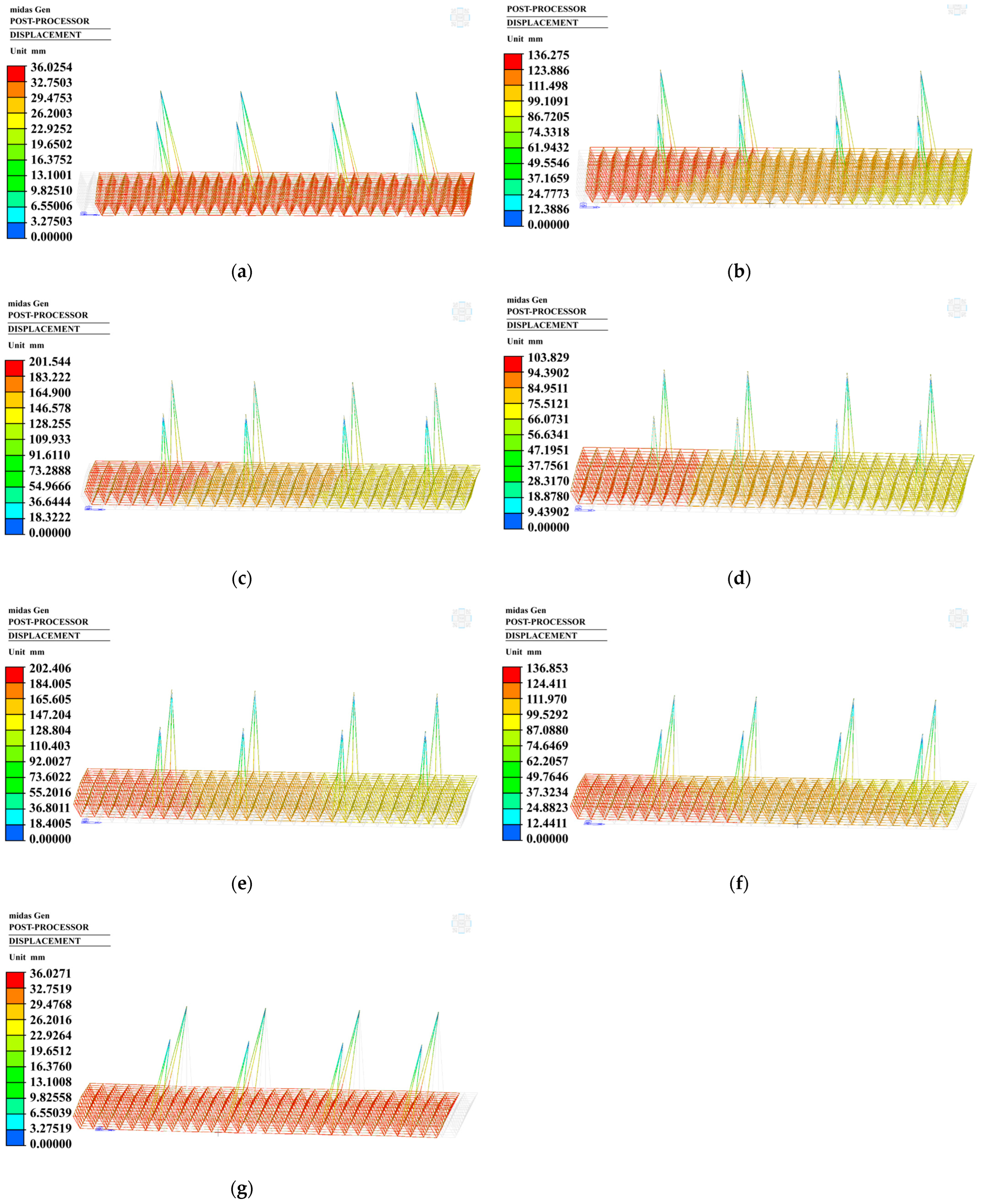
In the integral lifting process of large-span spatial steel frame, wind load is the dominant transverse dynamic excitation source, which has a decisive influence on the geometric displacement field and the redistribution of internal force of flexible suspension system. In view of the asymmetric arrangement of the lifting points of the roof space frame of Yanjiao Station, the traditional one-way wind pressure analysis cannot accurately reflect the complex aerodynamic response. The flow field interference effects under different wind directions show significant directionality and spatial heterogeneity. In order to quantitatively evaluate the wind load effect in the lifting stage, the piecewise incremental method based on the pre-defined wind field parameters was used to conduct a comprehensive numerical simulation of seven typical wind attack angles (0° to 180°) in Midas Gen software (2021, Midas Information Technology Co., Ltd., Seongnam, Republic of Korea). The structural response under different wind directions is visually displayed by the “load step-displacement” and “load step-stress” change curves (Figure 16), the displacement–stress relationship diagram (Figure 17), and the displacement contour map (Figure 18).

Analyses of Figure 16 and Figure 17 demonstrate that the space frame remains within the stable elastic regime under wind loading, with displacement and stress responses exhibiting pronounced directional sensitivity and a “bimodal evolution” pattern. The numerical results show that the peak response appears accurately at the oblique wind angles of 60° and 120° and the maximum displacement reaches 130 to 200 mm. In the face of 0°/180° longitudinal wind, the response amplitude is very small. This mechanical behavior is mainly due to the eccentric effect between the geometric center and the stiffness center caused by the asymmetric lift point. Under the action of oblique wind, this will cause serious eccentric bending moment and coupled translation–torsion response, thereby amplifying the second-order displacement of the cantilever end. In addition, the oblique wind will also increase the effective windward area. Combined with the low equivalent recovery stiffness of the flexible suspension system, the resulting overall geometric swing will lead to the redistribution of internal forces and significant stress concentration. In summary, 60° and 120° are identified as the key control conditions for the flexible suspension stage. With the change of wind direction angle, the structural deformation mode changes from symmetrical distribution to spatial asymmetric distribution, and the displacement field and stress field show a high spatial and temporal correlation.

5.3. Gray Relational Sensitivity Analysis of Safety Control Factors During Lifting

5.3.1. Selection of Behavioral Indicators and Orthogonal Simulation Scheme

To systematically evaluate the impact weights of ambient disturbances and incremental loading on the structural performance of the space frame during the critical “flexible suspension” phase of asymmetric hydraulic lifting, the Grey Relational Analysis (GRA) framework is implemented to execute a refined sensitivity analysis. Grounded in the prior multi-field coupling simulation datasets, three core control variables are decoupled: Lifting Instant Time (governing the transient thermal field evolution), Wind Angle of Attack (governing aerodynamic heterogeneity), and Wind Load Factor (governing the piecewise incremental nonlinear iteration). Under the translational–torsional coupling effects induced by the asymmetric lifting configurations, the geometric deformation mode typically precedes material strength failure. Consequently, Maximum Cantilever Displacement under coupled hazards is defined as the behavioral evaluation indicator.

Table 5. Average maximum cantilever displacement of the space frame under different control factors.

Factors	Level 1	Cantilever Disp./mm	Level 2	Cantilever Disp./mm	Level 3	Cantilever Disp./mm
Lifting Instant Time	08:00	187.70	12:00	189.10	14:00	192.50
Wind Attack Angle	0°	41.70	90°	103.98	120°	184.15
Wind Load Factor	0.3	51.20	0.6	104.00	1.0	184.20

tabulates the extracted average mechanical displacement responses at distinct levels.

5.3.2. Grey Relational Matrix Construction and Standardized Processing

To solve the relational trajectory from the numerical discrete solutions in Table 5, the independent variables are mapped into the comparative matrix X, while the corresponding maximum cantilever displacement responsive sequences are mapped into the reference matrix Y. The established mathematical expressions are structured as follows:

$$\mathrm{X}= {\left[x_{ij}\right]}_{\mathrm{m}\times \mathrm{n}}=\left[\begin{array}{cccc}{\mathrm{x}}_{11}& {\mathrm{x}}_{12}& \cdots & {\mathrm{x}}_{1\mathrm{n}}\\ {\mathrm{x}}_{21}& {\mathrm{x}}_{22}& \cdots & {\mathrm{x}}_{2\mathrm{n}}\\ ⋮& ⋮& \cdots & ⋮\\ {\mathrm{x}}_{\mathrm{m}1}& {\mathrm{x}}_{\mathrm{m}2}& \cdots & {\mathrm{x}}_{\mathrm{m}\mathrm{n}}\end{array}\right]=\left[\begin{array}{ccc}8.0& 12.0& 14.0\\ 0.0& 90.0& 120.0\\ 0.3& 0.6& 1.0\end{array}\right]\hspace{1em}$$

(10)

$$\mathrm{Y}={\left[y_{ij}\right]}_{m\times n}=\left[\begin{array}{cccc}{y}_{11}& y_{12}& \cdots & y_{1n}\\ y_{21}& y_{22}& \cdots & y_{2n}\\ ⋮& ⋮& \cdots & ⋮\\ y_{m1}& y_{m2}& \cdots & y_{mn}\end{array}\right]=\left[\begin{array}{ccc}187.70& 189.10& 192.50\\ 41.70& 103.98& 184.15\\ 51.20& 104.00& 184.20\end{array}\right]$$

(11)

where X and Y denote the tracking comparative matrix and reference responsive matrix, respectively. The mathematical dimensions and indices are defined as follows: m represents the total number of structural safety tracking indicators or behavior parameters (i = 1, 2, … m); n represents the total number of discrete data sampling nodes or observation times throughout the flexible suspension progression (j = 1, 2, … n); i is the specific parameter index that updates row vectors to isolate independent physical hazards; and j is the continuous time-series column index tracking the transient construction steps.

Owing to the inherent heterogeneity in physical dimensions and numerical scales among time, angle, and the load factor, the Min–Max Normalization operator is implemented to eliminate scaling constraints, transforming matrices X and Y into normalized domains:

$$x_{\mathit{ij}}^{\prime } = {\displaystyle \frac{x_{\mathit{ij}}-\underset{\mathrm{j}}{\min }\left(x_{\mathit{ij}}\right)}{\underset{\mathrm{j}}{\max }\left(x_{\mathit{ij}}\right)-\underset{\mathrm{j}}{\min }\left(x_{\mathit{ij}}\right)}}$$

(12)

$$y_{\mathit{ij}}^{\prime }={\displaystyle \frac{y_{\mathit{ij}}-\underset{\mathrm{j}}{\min }\left(y_{\mathit{ij}}\right)}{\underset{\mathrm{j}}{\max }\left(y_{\mathit{ij}}\right)-\underset{\mathrm{j}}{\min }\left(y_{\mathit{ij}}\right)}}$$

(13)

Executing linear mapping via the above formulas yields the scaled matrices x′ and y′. Consequently, the absolute deviations between the reference and comparative sequences at identical horizontal coordinates are calculated to establish the system-level difference sequence matrix Δ:

$$\Delta =\left[{\Delta }_{\mathit{ij}}\right]=\left[\left|y_{\mathit{ij}}^{\prime }-x_{\mathit{ij}}^{\prime }\right|\right]$$

(14)

Substituting the high-precision numerical discrete sequences yields the processed difference sequence matrix Δ:

$$\Delta ={\left[{\Delta }_{ij}\right]}_{m\times n}=\left[\begin{array}{cccc}{\Delta }_{11}& {\Delta }_{12}& \cdots & {\Delta }_{1\mathrm{n}}\\ {\Delta }_{21}& {\Delta }_{22}& \cdots & {\Delta }_{2\mathrm{n}}\\ ⋮& ⋮& \cdots & ⋮\\ {\Delta }_{m1}& {\Delta }_{m2}& \cdots & {\Delta }_{mn}\end{array}\right]=\left[\begin{array}{ccc}0.000& 0.192& 0.000\\ 0.000& 0.113& 0.000\\ 0.000& 0.030& 0.000\end{array}\right]$$

(15)

where $\Delta$ represents the discrete matrix elements of absolute deviations computed as $\Delta =\left[{\Delta }_{\mathit{ij}}\right]=\left[\left|y_{\mathit{ij}}^{\prime }-x_{\mathit{ij}}^{\prime }\right|\right]$ to map structural irritations.

5.3.3. Relational Coefficient and Sensitivity Index Calculation

Utilizing the difference sequence matrix Δ as the primal data source, the localized gray relational coefficients L_ij at each discrete node are solved as follows:

$$L_{ij}={\displaystyle \frac{{\Delta }_{\mathit{min}}+\rho \cdot {\Delta }_{\mathit{max}}}{{\Delta }_{ij}+\rho \cdot {\Delta }_{\mathit{max}}}}$$

(16)

where ${\Delta }_{\mathit{min}}$ is the global minimum within matrix Δ(${\Delta }_{\mathit{min}}$ = 0.000) and ${\Delta }_{\mathit{max}}$ is the global maximum (${\Delta }_{\mathit{max}}$ = 0.192). $\rho$ denotes the distinguishing coefficient, which is assigned as $\rho$ = 0.5 in compliance with international standard practices in structural wind engineering and safety evaluation paradigms.

Through matrix transformations, the gray relational coefficient matrix L is derived. To quantitatively judge the weight of each environmental disturbance and incremental step affecting the structural geometric stability, the arithmetic mean of the coefficients along the horizontal level coordinates is determined, yielding the final gray relational grade (sensitivity index) matrix $Q_i$:

$$Q_i={\displaystyle \frac{1}{\mathrm{n}}}{\sum }_{\mathrm{j}=1}^{\mathrm{n}}{\mathrm{L}}_{\mathrm{i}\mathrm{j}}$$

(17)

The sensitivity index $Q_i$ ∈ [0, 1] serves as the primary metric for evaluating the disturbance intensity of external variables. A value of ${\mathrm{Q}}_{\mathrm{i}}$ closer to 1 implies that fluctuations in this specific factor possess a powerful capacity to irritate cantilever deformations, designating high structural sensitivity. Conversely, a value near 0 denotes prominent geometric robustness against the specific field disturbance. Through global continuous iterations of the system, the calculated sensitivity indexes ${\mathrm{Q}}_{\mathrm{i}}$ for each control factor are explicitly obtained as

$$\begin{gathered} Q_i=\left[Q_t, Q_{\theta }, Q_{\lambda }\right] \\ =\left[0.551, 0.592, 0.883\right] \end{gathered}$$

(18)

According to the analytical deductions, the sensitive indexes are explicitly output as follows: Wind Load Factor is 0.883, Wind Angle of Attack is 0.592, and Lifting Instant is 0.551.

5.3.4. Factor Sensitivity Ranking and Proactive Construction Control Strategies

To provide a clearer hierarchy of the dominant hazards threatening the floating space frame, a concise quantitative sensitivity ranking of the key governing parameters is established based on the computed system gray relational grades (Qi). The rigorous numerical sequence governing the structural safety margin during the asymmetric hoisting phase is explicitly prioritized as follows: Wind Load Intensity ($Q_{\lambda }$ = 0.883) > Asymmetric Lifting Configuration and Eccentricity ($Q_{\theta }$ = 0.592) > Non-Uniform Temperature Gradient (${ Q}_t$ = 0.551). This quantitative ranking firmly indicates that the transient lateral wind pressure operates as the absolute dominant dynamic excitation controlling the peak cantilever displacement fields, closely coupled with the structural center of mass stiffness eccentricity natively instigated by the asymmetric boundary configurations. Concurrently, the time-varying non-uniform solar thermal gradient serves as a prominent background modulation factor that further amplifies the secondary structural deformation amplitudes. Consequently, during active on-site pre-control implementations, mitigating the structural eccentricities via geometric alignment and strictly avoiding peak wind-vulnerable attack angles (60°/120°) must be designated as top-tier safety actions.

6. Time-Varying Mechanical Performance and Critical Load Case Identification of the Space Frame Under Coupled Thermal and Wind Fields

The influence of non-uniform thermal field and isolated wind load on the mechanical properties of the spatial frame of Yanqiao station has been discussed in a previous paper, and the structural sensitivity under various environmental loads has been clarified. However, in the actual lifting construction environment, the thermal field and the wind field do not change independently but show complex time–space coupling characteristics. Based on the characteristic parameters determined by the previous analysis, this study uses orthogonal experimental design to evaluate the coupled load conditions. In order to meet the requirements of extreme condition identification in the safety control of large-span steel structures, a quasi-decoupling analysis method is adopted in this study. This calculation strategy aligns with the mechanical philosophy of stiffness separation and partial modeling methodologies widely leveraged in long-span truss assemblies to isolate regional nonlinear disturbances [40]. Specifically, the method captures the nonlinear behavior of the structure by quasi-decoupling: first, the structural state under solar radiation is solved as the initial geometric configuration, and then the wind load is applied and solved using the Newton–Raphson nonlinear iteration method to consider the second-order effect. The applicability and physical validity of this sequential quasi-decoupled framework are firmly governed by two decoupled structural mechanisms: time-scale separation and asymmetric boundary feedback. Mechanically, the solar-induced non-uniform thermal evolution is a transient slow-variational phenomenon operating on an hourly macro-scale, whereas the wind-induced structural vibration operates as a high-frequency dynamic fluctuation on a multi-second micro-scale. Furthermore, thermodynamic pre-deformation acts as a dominant driver that noticeably updates the geometric stiffness matrix for subsequent aerodynamic calculations. In contrast, the spatial micro-swings and transient vibrations triggered under a Grade 6 wind threshold generate negligible physical feedback on the ambient convective heat coefficients, thermal conductivity matrix, or the component solar interception cross-sections calculated via the AABB coordinates. Consequently, this strategy can accurately determine the mechanical response range under the most critical load combination, thus providing a highly efficient and conservative safety margin for construction monitoring.

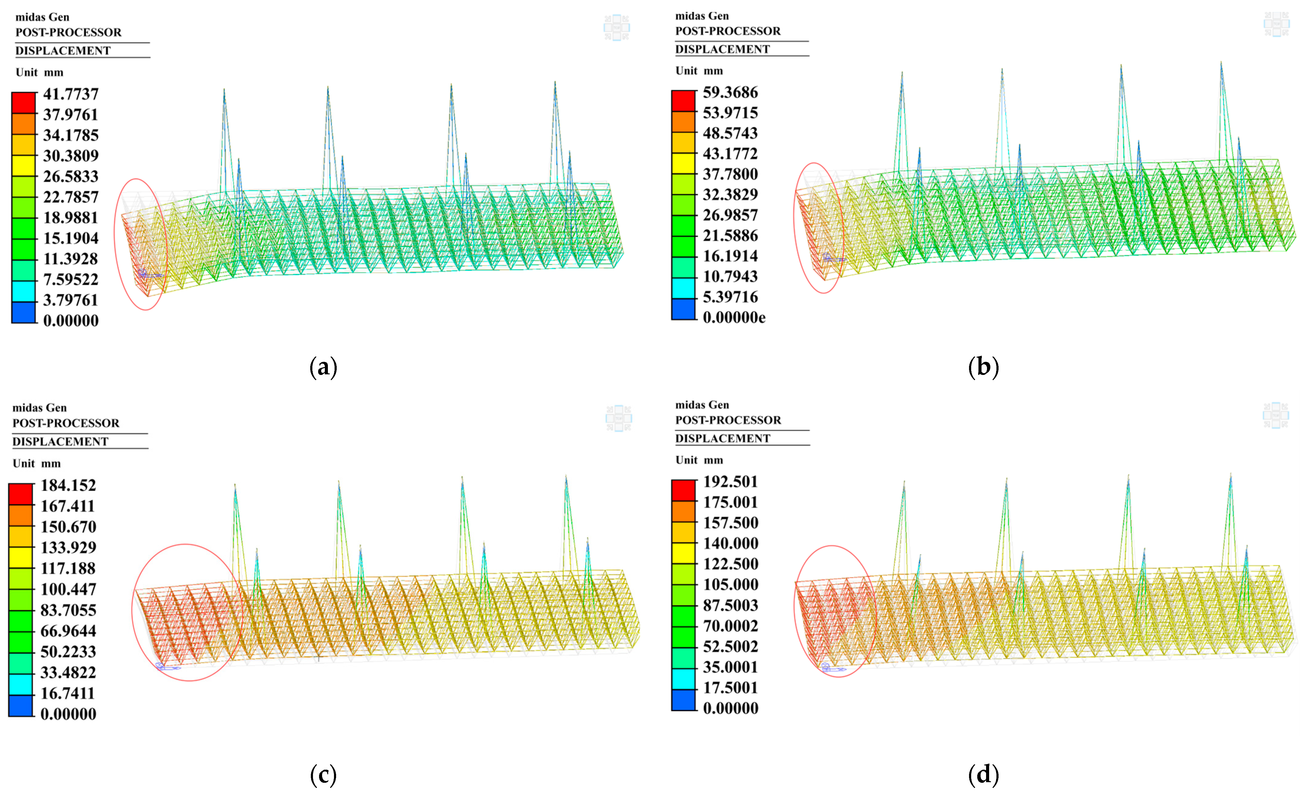
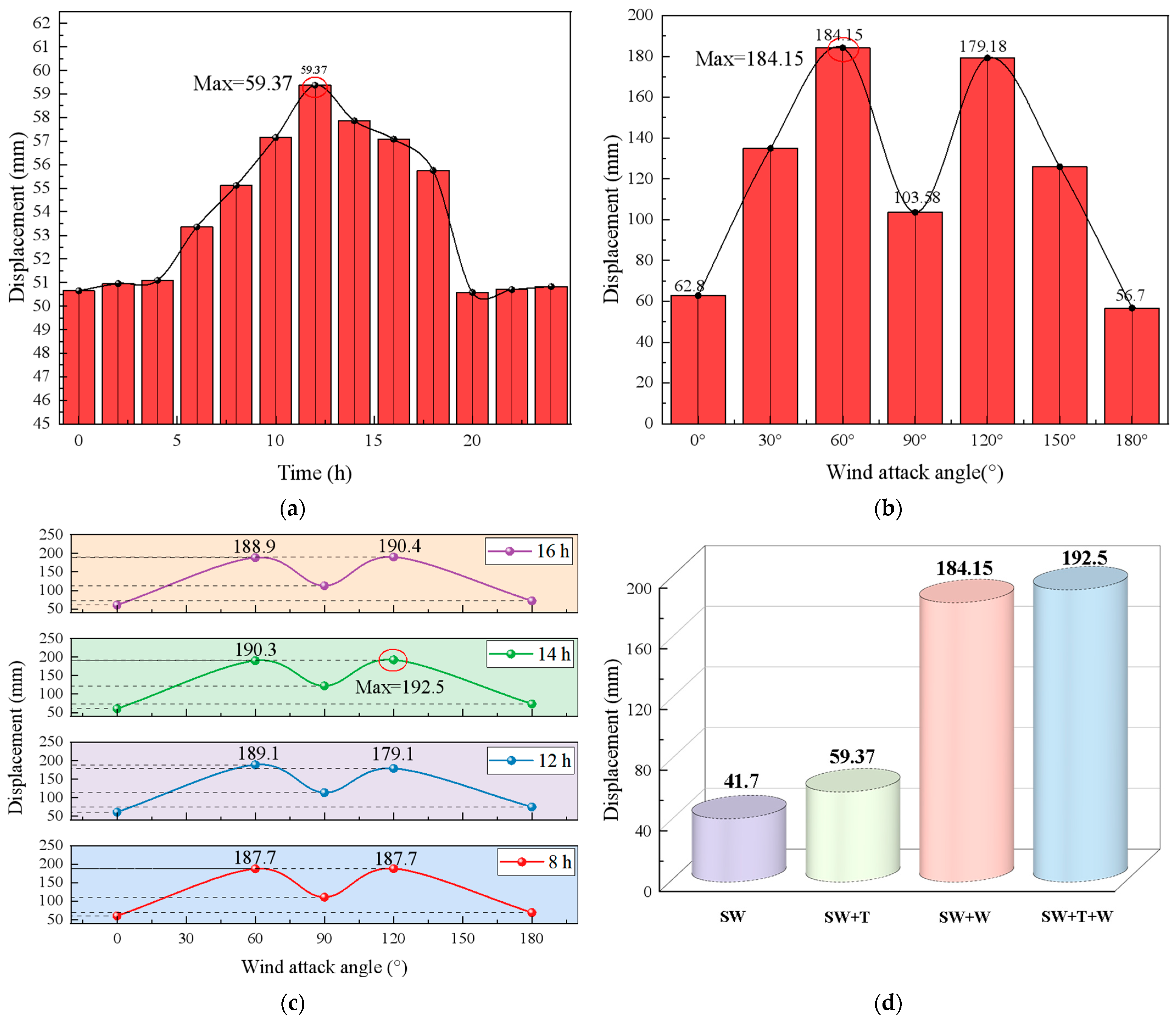
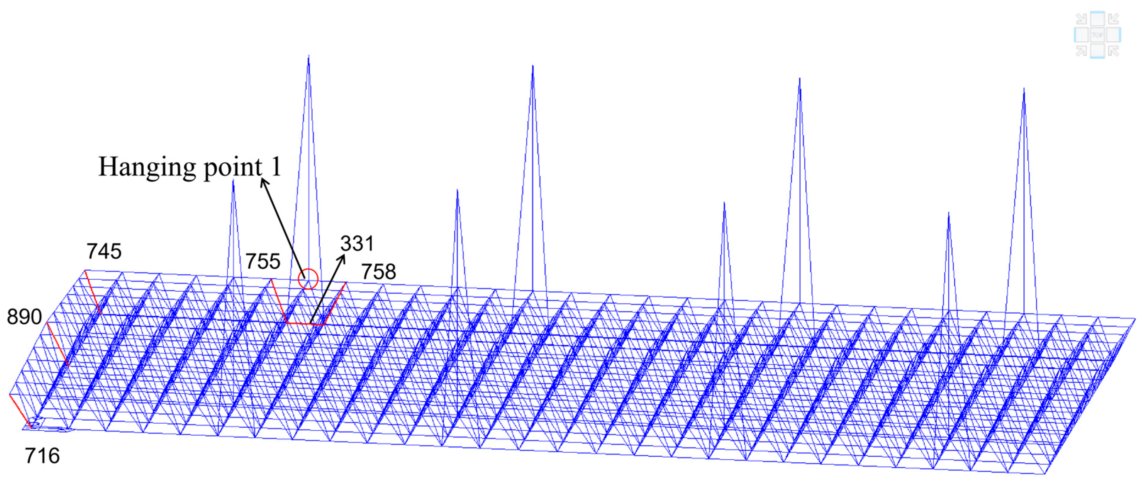
In order to study the structural response under the coupling of hot and wind, we selected four key time nodes in the thermal evolution process: the start time of rapid heating (08:00), the absolute maximum temperature point (12:00), the maximum thermal non-uniformity point (14:00), and the continuous high temperature stage (16:00). Combined with the wind load response characteristics, five representative wind attack angles (0°, 60°, 90°, 120°, 180°) were selected. Using these variables, a full-factor parametric study including 20 coupled load conditions was constructed. Through the comprehensive analysis of the displacement time history curve, the comparison of extreme values (Figure 19) and the displacement contour map (Figure 20), it can be seen that the wind load causes the high deformation area to shift significantly to the direction of lifting point 1. In order to further explore the mechanical evolution process, we extracted the stress data of the key compression members (i.e., members 716, 890, 745, 331, 755, and 758 near the cantilever section and lifting point 1; see Figure 21) (

Table 6. Peak compressive stress of key structural members under different load cases (MPa).

Location	Element ID	Dead Load	Dead + Temp	Dead + Wind	Dead + Temp + Wind
Cantilever End	716	4.73	5.20	4.94	4.90
	745	4.92	5.27	5.171	5.18
	890	4.18	5.07	4.522	4.55
Near Lifting Point 1	331	86.50	99.22	130.12	123.27
	755	31.10	36.26	36.48	39.08
	758	32.11	35.56	43.73	36.03

). The experimental scheme aims to clarify the dynamic superposition mechanism between the thermally induced initial deformation and the wind pressure change at multiple angles of attack and systematically reveal the internal force redistribution and geometric evolution of the flexible suspension system in the extreme coupling environment. These research results provide a solid numerical basis and scientific guidance for the safety risk assessment and improvement scheme optimization of large-span spatial frames in complex construction environments.

Through the comparative analysis of four load conditions—constant load, constant load + heat load, constant load + wind load and heat–wind coupling—it is found that the maximum structural displacement gradually increases with load complexity, reaching a peak (192.50 mm) under the fully coupled condition (Figure 19). The displacement response is mainly driven by wind load, which is 360.81% higher than the reference value of dead load. The stress evolution analysis shows that the area near lifting point 1 is the strength control area; the compressive stress in this area exceeds 130 MPa under wind load (Table 6), showing a significant nonlinear load superposition effect. From a mechanical point of view, the low stiffness of the asymmetric cantilever structure makes it a permanent weak link in energy dissipation. As a non-conservative force, the wind field continuously changes the mechanical vibration mode of the structure through aerodynamic work. The thermal field induces geometric deformation through thermal strain. The synergistic superposition effect of the two significantly amplifies the structural response. The results show that the wind load is the main factor controlling the structural mechanical response during the lifting process, which determines the response distribution characteristics. The thermal field mainly affects the response amplitude. In view of the correlation between the wind sensitive angle (60°/120°) and the maximum temperature in the afternoon, it is suggested to adopt the “peak avoidance” strategy in construction and give priority to the early morning period when the temperature and wind speed are low so as to ensure the safety and stability of the asymmetric lifting operation.

In order to strengthen the strategy, the system adopts a hierarchical early warning mechanism: when the cantilever displacement reaches 150 mm or the peak compressive stress of the key component exceeds 100 MPa, a first-level alarm will be triggered.

• This threshold is set because 150 mm corresponds to the lower limit of the high displacement sensitive area (130–200 mm) (defined by the translation–torsion coupling effect caused by 60°/120° wind force). To promptly capture this translational–torsional behavior, a multi-scale monitoring frequency is implemented. An hourly sampling interval is executed during routine static thermal cycles, which automatically switches to a high-frequency real-time dynamic sampling mode (10–20 Hz) when wind boundaries approach critical construction limits.
• The stress limit of 100 MPa provides the necessary safety margin, which can effectively deal with the peak compressive stress measured by the key components near the lifting point 1 exceeding 130 MPa. High-precision fiber optic or strain sensors are strategically deployed at these core vulnerable coordinates to continuously track internal force redistribution throughout the transient flexible suspension phase.

7. Applicability and Generalization of the Methodology Framework

The coupled thermal–wind structural safety tracking framework and the dual-dimensional pre-control strategy established in this study exhibit robust engineering scalability and can be generalized to alternative large-span structural systems, geometric topologies, lifting configurations, and climatic regions. Mathematically, the execution of automated non-uniform solar thermal mapping based on the Axis-Aligned Bounding Box (AABB) grid algorithm and localized CFD aerodynamic boundary tracking is independent of specific geometric shapes. Consequently, for alternative long-span structural typologies—such as spatial steel truss assemblies, large-span arch bridges, or grid composite domes—the core framework can be effectively implemented by updating the spatial bounding box arrays and localized shape wind pressure boundaries to accurately capture transient multi-field responses.

Furthermore, the methodology remains highly effective across different construction lifting boundaries and environmental configurations. In synchronous symmetric lifting operations or multi-point, multi-stage staging hoisting configurations, the evaluation reference matrix and comparative matrix can be flexibly adjusted to reflect modified leveling tracking variables or structural stiffness eccentricities. When extending this framework to distinct microclimatic zones—such as coastal regions characterized by typhoon hazards, tropical zones with intense solar intensities, or inland areas subjected to severe freeze-thaw temperature drops—the localized thermal and aerodynamic boundaries can be generalized using regional meteorological statistics and building design codes. By executing this comprehensive analytical loop, the temporal sensitivity sequences and dynamic thresholds can be rapidly extracted for generic structures, demonstrating the extensive practical usefulness and cross-platform transferability of the proposed methodology.

8. Conclusions

This study systematically quantified the dynamic responses of the Yanjiao Station large-span space frame during critical construction phases through refined numerical simulations of thermo-wind coupled effects. The primary conclusions are as follows:

• Under the dynamic interplay of solar radiation and local shading effects, the space frame exhibits a non-uniform transient thermal field. Nodal vertical constraints limit free thermal expansion, inducing a peak component temperature of approximately 34 °C and a maximum stress of 9.18 MPa localized at the sunward cantilever chords at 12:00. Furthermore, a distinct 3 h thermal lag is captured, with the overall average structural temperature peaking at 14:00.
• The wind-induced structural response demonstrates a pronounced directional sensitivity, evolving in a distinct “bimodal” pattern relative to the wind attack angle. The critical aerodynamic thresholds are precisely localized at oblique wind angles of 60° and 120°, driving the maximum displacement up to the 130–200 mm regime, whereas longitudinal wind components (0°/180°) prompt trivial responses.
• The inherent eccentricity between the structural center of mass and the center of stiffness—instigated by the asymmetric lifting point layout—is the root cause of translational–torsional coupling and second-order geometric amplification. In the multi-field environment, the wind field governs the spatial deformation mode, while the non-uniform thermal field dynamically amplifies the amplitude. This synergy pushes the absolute peak displacement to 192.50 mm under full coupling, which is 360.81% higher than the dead load baseline.
• The cantilever end and the strength core near Lifting Point 1 are identified as the primary vulnerable zones. To shift management from passive monitoring to active pre-control, a multi-dimensional early warning strategy is established: a First-Level Alarm is triggered when the cantilever displacement reaches 150 mm or the peak compressive stress of critical members exceeds 100 MPa based on high-vulnerability sensor deployment and multi-scale (hourly to 10–20 Hz) monitoring frequencies. Construction operations should strictly avoid the afternoon peak hours and prioritize the early morning window characterized by low thermal gradients and minimal wind velocity.

Finally, while the implemented quasi-static wind load configuration provides a computationally efficient and conservative boundary control for the current structural safety evaluations, it represents a simplified macro-scale approach. Consequently, investigating potential dynamic amplification effects, stochastic gust-induced transient responses, and intricate high-fidelity wind–structure interaction (WSI) mechanisms under reduced boundary constraints constitutes a path forward and inspiration for our next-stage deep exploration. Future research will focus on developing nonlinear aeroelastic coupled grids to further improve the dynamic pre-control precision of large-span spatial frameworks during their transient construction phases.

References

1. Szafran, J.; Juszczyk, K.; Kamiński, M. Coupled finite volume and finite element method analysis of a complex large-span roof structure. Int. J. Appl. Mech. Eng. 2017, 22, 995–1017. [Google Scholar] [CrossRef]
2. Zhang, M.; Chen, Y.; Zhou, P.; Zhuang, Z. Application of overall lifting technology in the construction of large-span steel truss. Steel Constr. 2018, 33, 94–98. [Google Scholar] [CrossRef]
3. Chen, Z.; Tang, J.; Tang, X.; Wu, H.; Gu, J.; Gu, J. Research on hydraulic synchronous overall lifting construction technology of large-span steel truss roof. Build. Constr. 2024, 46, 1884–1887. [Google Scholar] [CrossRef]
4. Su, H.; Wang, J.; Ding, S.; Li, J.; Yi, Z. Study on multi-point asymmetric overall lifting technology of large-span space special-shaped surface steel truss structure based on cloud monitoring. Ind. Constr. 2020, 50, 105–115. [Google Scholar] [CrossRef]
5. Shi, K. Key Construction Technology of Large-Span Space Arch Truss Steel Roof Structure Lifting. Ph.D. Thesis, South China University of Technology, Guangzhou, China, 2020. [Google Scholar] [CrossRef]
6. Wang, S.; Yan, R.; Yan, C.; Zou, Y.; Zhu, M. Optimization analysis of intermediate control target parameters during construction of large-span space grid structure. Space Struct. 2024, 30, 59–69. [Google Scholar] [CrossRef]
7. Tu, X. Application and design of hydraulic synchronous overall lifting technology for large steel trusses. Mech. Res. Appl. 2020, 33, 109–111. [Google Scholar] [CrossRef]
8. Formisano, A.; Ahmadi, H.M.; Mazzolani, F.M. Ductility and behaviour factor of RC frame-perforated SPSW dual systems. Key Eng. Mater. 2018, 763, 835–845. [Google Scholar] [CrossRef]
9. Zhou, M.; Fan, J.S.; Liu, Y.F.; Zhang, J.-X.; Duan, X.-J.; Lei, S.-S. Non-uniform temperature field and effect on construction of large-span steel structures. Autom. Constr. 2020, 119, 103339. [Google Scholar] [CrossRef]
10. Xu, W.; Chen, D.; Qian, H.; Chen, W. Non-uniform temperature field and effects of large-span spatial truss structure under construction: Field monitoring and numerical analysis. Structures 2021, 29, 416–426. [Google Scholar] [CrossRef]
11. Jiang, P. Study of temperature field in large-span steel structure under radiation-thermal-fluid coupling. Arch. Civ. Eng. 2023, 69, 661. [Google Scholar] [CrossRef]
12. Song, S.; Qian, J.; Zhou, L. Temperature Field and Gradient Effects for Concrete-Filled Steel Tubular Truss Arch Bridges Under Construction. Buildings 2026, 16, 969. [Google Scholar] [CrossRef]
13. Zhao, R.; Liu, Q.; Wang, H.; Ma, G. Determination of temperature action values and most unfavorable working conditions for grid structures. Ind. Constr. 2023, 53, 88–93. [Google Scholar] [CrossRef]
14. Wang, Y.; Zhou, Q. Evaluation method for key members of steel grid structures under high temperature. Build. Struct. 2021, 51, 539–542. [Google Scholar]
15. Yang, K.; Zhang, W.; Chen, R.; Duan, M.; Shangguan, H. Simulation analysis of temperature field and stress field of mass concrete under different construction temperatures. Buildings 2025, 15, 370. [Google Scholar] [CrossRef]
16. Prabhakara Rao, P.; Sampath, V. CFD analysis on airfoil at high angles of attack. Int. J. Eng. Res. 2014, 3, 430–434. [Google Scholar] [CrossRef]
17. Yu, H. Study on Wind-Induced Loads and Related Characteristics of Tall Building Groups Based on Synchronous Pressure Measurement Technology. Master’s Thesis, Shantou University, Shantou, China, 2010. [Google Scholar]
18. Fu, J.Y.; Gao, Y.; Wu, J.R.; Xu, A. Wind effects on a long span steel roof structure: Numerical simulation and equivalent static wind loads. J. Vibroeng. 2015, 17, 2572–2590. [Google Scholar]
19. Ruan, R.; Lai, M.; Jiang, C.; Wang, J.; Lin, Y. Integral lifting of steel structure corridor between two super high-rise buildings under wind load. Buildings 2023, 13, 2441. [Google Scholar] [CrossRef]
20. Tang, H.; Li, Y.; Wang, Y.; Tao, Q. Aerodynamic optimization for flutter performance of steel truss stiffening girder at large angles of attack. J. Wind Eng. Ind. Aerodyn. 2017, 168, 260–270. [Google Scholar] [CrossRef]
21. Qiu, Y.; Yu, R.; San, B.; Li, J. Aerodynamic shape optimization of large-span coal sheds for wind-induced effect mitigation using surrogate models. Eng. Struct. 2022, 253, 113818. [Google Scholar] [CrossRef]
22. Li, Y.; Zhao, H. Spatial Wind Flow Load and Shape Optimization for Folding Grid Shell Buildings. IEEE Access 2023, 11, 135304–135322. [Google Scholar] [CrossRef]
23. Wu, X.; Chen, S.; Hu, Y.; Wang, Z.; Li, Z. Analysis and real-time monitoring of the influence of wind load on a high-altitude steel connecting bridge with small spacing. Buildings 2024, 14, 1755. [Google Scholar] [CrossRef]
24. Lu, L.; Zheng, L.; Yan, S. Numerical simulation and research on wind load of large-span steel tube truss structure. Theory Res. Urban Constr. 2014, 32, 92–93. [Google Scholar] [CrossRef]
25. Chen, X.; Yu, H.; Yu, H.; Zhao, P.; Li, M. Aerodynamic Loading and Wind-Induced Vibration Characteristics of Bridge Girders with Typical Asymmetric Configurations. Buildings 2025, 15, 2824. [Google Scholar] [CrossRef]
26. Han, M.; Yang, B.; Gao, X.; Jiang, J.; Han, R. -induced Response and Vibration Damping Analysis of Large-span Grid Structures Considering Fluid–structure Interaction. Int. J. Steel Struct. 2026, 26, 86–98. [Google Scholar] [CrossRef]
27. Kafshgarkolaei, H.J.; Lotfollahi-Yaghin, M.A.; Mojtahedi, A. A modified orthonormal polynomial series expansion tailored to thin beams undergoing slamming loads. Ocean Eng. 2019, 182, 38–47. [Google Scholar] [CrossRef]
28. Zhou, J.; Zhang, M.; Wang, Y. A Case Study on Response Characteristics of Large Steel Frame Support Structures Under the Combined Action of Earthquake and Wind Loads, Considering Shielding Effects. Buildings 2026, 16, 1644. [Google Scholar] [CrossRef]
29. Zhang, Y.; Chen, Z.; Yang, S. Elasto-plastic stability analysis of large-span steel grid dome structures. J. Civ. Environ. Eng. 2022, 44, 189–196. [Google Scholar] [CrossRef]
30. Chandrasiri, D.; Gatheeshgar, P.; Ahmadi, H.M.; Simwanda, L. Numerical study of thermal efficiency in light-gauge steel panels designed with varying insulation ratios. Buildings 2024, 14, 300. [Google Scholar] [CrossRef]
31. Mao, Y.; Xiao, F.; Tian, G.; Xiang, Y. Sensitivity analysis and sensor placement for damage identification of steel truss bridge. Structures 2025, 73, 108310. [Google Scholar] [CrossRef]
32. Cooper, P.I. The absorption of radiation in solar stills. Sol. Energy 1969, 12, 333–346. [Google Scholar] [CrossRef]
33. Kehlbeck, F. Effect of Solar Radiation on Bridge Structure; Liu, X.F., Translator; Chinese Railway Publishing Company: Beijing, China, 1981. [Google Scholar]
34. Liu, B.Y.H.; Jordan, R.C. The interrelationship and characteristic distribution of direct, diffuse and total solar radiation. Sol. Energy 1960, 4, 1–19. [Google Scholar] [CrossRef]
35. Kasten, F.; Young, A.T. Revised optical air mass tables and approximation formula. Appl. Opt. 1989, 28, 4735–4738. [Google Scholar] [CrossRef] [PubMed]
36. Zhou, M.; Fan, J.S.; Liu, Y.F.; Zhang, J.; Duan, X.; Lei, S. Study on non-uniform temperature field of steel grid structure in the core area of Beijing Daxing International Airport Terminal. Eng. Mech. 2020, 37, 46–54. [Google Scholar] [CrossRef]
37. Yang, S.; Tao, W. Heat Transfer, 5th ed.; Higher Education Press: Beijing, China, 2019. [Google Scholar]
38. Yang, S.M.; Tao, W.Q. Heat Transfer, 4th ed.; Higher Education Press: Beijing, China, 2006. [Google Scholar]
39. GB 50009-2012; Ministry of Housing and Urban-Rural Development of the People’s Republic of China. Load Code for the Design of Building Structures. China Architecture & Building Press: Beijing, China, 2012.
40. Xiao, F.; Mao, Y.; Tian, G.; Chen, G.S. Partial-model-based damage identification of long-span steel truss bridge based on stiffness separation method. Struct. Control Health Monit. 2024, 2024, 5530300. [Google Scholar] [CrossRef]
Figure 1. Panoramic view of the Yanjiao Railway Station. The Chinese characters “燕郊站” represent Yanjiao Railway Station.
Buildings 16 02669 g001
Figure 2. Tructural configuration of the Yanjiao Station roof space frame. (a) 3D spatial schematic of the orthogonally placed square pyramid framework. (b) Engineering design blueprints detailing planar axis layout and elevation control dimensions.
Buildings 16 02669 g002
Figure 3. Front elevation detailing the asymmetrical synchronous lifting point configuration for the space frame.
Buildings 16 02669 g003
Figure 4. Schematic of the Yanjiao Station space frame during the flexible suspension stage.
Buildings 16 02669 g004
Figure 5. Geometric relationship between incident solar rays and an arbitrarily inclined surface.
Buildings 16 02669 g005
Figure 6. Coordinate transformation between the ray coordinate system (oxyz) and the global coordinate system (OXYZ). Adapted with permission from Ref. [36]. Copyright 2020, Eng. Mech.
Buildings 16 02669 g006
Figure 7. Schematic of the bounding box detection method. Adapted with permission from Ref. [36]. Copyright 2020, Eng. Mech.
Buildings 16 02669 g007
Figure 8. Determination of shading relationships between structural components.
Buildings 16 02669 g008
Figure 9. Calculation of shaded regions on circular tubular members under solar radiation. Adapted with permission from Ref. [36]. Copyright 2020, Eng. Mech.
Buildings 16 02669 g009
Figure 10. Temporal evolution trends of structural element temperatures.
Buildings 16 02669 g010
Figure 11. Temperature field distribution of structural members at representative time steps (time: Beijing Standard Time, UTC+8; simulation parameters correspond to the previously mentioned typical day to represent peak solar radiation intensity): (a) 4 h; (b) 8 h; (c) 12 h; (d) 14 h; (e) 16 h; (f) 20 h.
Buildings 16 02669 g011
Figure 12. Comparative analysis of finite element results between Midas Gen and Ansys platforms: (a) MIDAS Gen computational results; (b) ANSYS computational results.
Buildings 16 02669 g012
Figure 13. Comparison between simulated and measured lifting forces at Lifting Point 1.
Buildings 16 02669 g013
Figure 14. Temporal relationships between structural displacements, stresses, and the non-uniform thermal field.
Buildings 16 02669 g014
Figure 15. Displacement and stress distributions under the non-uniform thermal field at 12:00. (a) Displacement field distribution; (b) von Mises stress distribution.
Buildings 16 02669 g015
Figure 16. Evolution curves of structural response under varying wind attack angles. (a) Load step–displacement curves. (b) Load step–stress curves. (The lines for 0° and 180° are nearly overlapped. The black dashed line on the 180° line is the curve for 0°).
Buildings 16 02669 g016
Figure 17. Relationship between structural displacements, stresses, and wind attack angles.
Buildings 16 02669 g017
Figure 18. Structural displacement contours under different wind attack angles: (a) 0°; (b) 30°; (c) 60°; (d) 90°; (e) 120°; (f) 150°; (g) 180°.
Buildings 16 02669 g018
Figure 19. Comparative analysis of coupling load cases. (a) Dead load + thermal. (b) Dead load + wind. (c) Dead load + thermal + wind. (d) Maximum displacement comparison across load cases.
Buildings 16 02669 g019
Figure 20. Displacement contour plots for the most unfavorable scenarios under various coupling conditions. (a) Dead load. (b) Dead load + thermal (12 h). (c) Dead load + wind (60°). (d) Dead load + thermal (14 h) + wind (120°). (The area marked by the red circle is the overhanging region with large structural displacement, which corresponds to the most unfavorable position of the structure).
Buildings 16 02669 g020
Figure 21. Spatial distribution of key compressive structural members.
Buildings 16 02669 g021