Performance-Based Probabilistic Post-Earthquake Assessment Method for Structural Health Monitoring and Its Implementation on the Old Hall of Nanjing Museum

Abstract

The assessment of post-earthquake performance of structures is a crucial task in structural health monitoring. To address this challenge, a novel performance-based probabilistic post-earthquake assessment (PBPPA) method is proposed. This method involves a modeling stage and an application stage. First, twenty earthquake waves with fortification intensity and rare intensity are selected from the PEER (Pacific Earthquake Engineering Research Center) database, and the mean and standard deviation are consistent with the target values. Then, OpenSEES is used to establish a finite-element model for the monitored structure. Next, the damage state and performance measures of structural elements are calculated according to the standard for seismic resilience assessment of buildings. Finally, the conditional probability density function of the repair cost relative to the monitoring data is presented, along with a probabilistic rating method of three levels. Using the Old Hall of Nanjing Museum as an example, the proposed method is verified with numerical simulation and real-world monitoring data collected during earthquakes. It is found that the most likely occurring repair cost and deviation of the conditional probability density function are proportional to the intensity of dynamic responses, which is consistent with the actual situation. Therefore, the presented method can be used as the decision-making basis for the determination of the structural post-earthquake condition and provides a useful reference for the future development of post-earthquake assessment methods. Overall, the proposed method is a valuable contribution to the field of structural health monitoring and has the potential to enhance the safety and resilience of structures after earthquakes.

1. Introduction

Earthquakes are among the potential risks posing a significant hazard to the safety and integrity of civil engineering structures. Upon experiencing an earthquake event, these structures are prone to suffer various degrees of damage, leading to a deterioration in their seismic performance over the short or long term [1]. Therefore, the prompt acquisition of post-earthquake damage conditions and associated consequences becomes imperative for informed decision-making regarding rescue operations and maintenance. Within the research field of SHM (structural health monitoring), the accurate and rapid assessment of structural damage conditions after earthquakes has emerged as a crucial and challenging topic.

For civil engineering structures, damage can occur over varying time scales. It can be accumulated incrementally over a long period of time due to fatigue or corrosion. Alternatively, damage can be triggered abruptly within a relatively short period of time due to extreme events like earthquakes [1]. Therefore, SHM can be categorized into two distinct domains based on the monitoring scales, namely long-term monitoring and short-term monitoring. Long-term monitoring primarily focuses on assessing damage accumulation over an extended duration [2,3,4]. During this process, the excitation sources are typically ambient and characterized by stable stochastic processes. This assumption of stability in the excitation process is critical for the development and implementation of effective vibration-based algorithms for long-term damage detection [5,6,7,8]. However, it is important to note that this assumption of stable stochastic processes is no longer applicable in the case of short-term monitoring algorithms. In short-term monitoring, where damage is induced suddenly, the excitation sources are no longer stable as assumed previously. Therefore, the algorithms employed for short-term monitoring need to adapt to this dynamic nature of the excitation process to ensure accurate and reliable post-event assessment.

Post-earthquake assessment falls into the category of short-term monitoring. Currently, there are mainly three types of post-earthquake assessment methods: vibration-based, vision-based, and their combination. Vibration-based methods involve the collection of dynamic response data from monitored structures during earthquakes. These methods focus on extracting damage-sensitive features from the collected vibration data for subsequent analysis. Frequently used features include time-domain features like maximum inter-story drift angle [9,10], and frequency domain features like instantaneous frequency [11]. The extracted features are then correlated with different damage levels, enabling the prediction of damage severity based on the collected vibration data [12,13,14]. On the other hand, vision-based methods rely on acquiring imagery of structures or regions utilizing various imaging technologies such as LiDAR (light detection and ranging) [15], satellite imagery [16,17,18], UAV (unmanned aerial vehicle) [17,19], and PolSAR (polarimetric synthetic aperture radar) [20], etc. Then the damage assessment of monitored structures is conducted by comparing the features extracted from the collected pre- and post-earthquake imagery. Another type of post-earthquake assessment method attempts to exploit the combination of different sources of information [21]. This approach integrates both vibration and vision data through data fusion techniques, allowing for a comprehensive assessment of the damage. With the growing number of structures that are equipped with SHM systems [22], the acquisition of real-time vibration data has become more readily available, enabling a convenient implementation of the vibration-based post-earthquake assessment methods.

Despite the aforementioned studies and applications about post-earthquake assessment methods, several challenges persist, including: (1) Vision-based methods, while effective in detecting significant deformations and fractures in structures following large earthquakes, encounter difficulties in promptly inspecting potential damage after small earthquakes. Moreover, these methods often require more time for the capture and processing of post-earthquake images than vibration-based methods, potentially causing delays in decision-making. (2) Most existing vibration-based methods primarily focus on calculating post-earthquake damage levels without providing comprehensive performance-based consequences. Thus, there is a need to develop methods that can assess the performance implications of the observed damage. (3) It is essential to accurately account for the stochastic nature of earthquake events in order to provide more robust and reliable assessments. The inherent randomness and variability of earthquake intensity necessitate a quantification and incorporation of these factors into the post-earthquake assessment results.

In light of the aforementioned considerations, this paper proposes a performance-based probabilistic post-earthquake assessment (PBPPA) method for monitored structures. Unlike conventional vibration-based post-earthquake assessment methods, which mainly use dynamic response features to identify or classify structural damage, the proposed method further links monitored structural responses with performance-based consequences, represented by repair cost in this study. In addition, different from deterministic damage-level evaluation approaches, the proposed method explicitly considers the uncertainty associated with earthquake excitations and nonlinear structural responses by establishing a joint probabilistic model between engineering demand features and performance measures. Once earthquake-induced monitoring data are obtained, the conditional probability distribution of the repair cost can be derived, and the probabilities associated with different risk levels can be evaluated. This framework enables post-earthquake assessment results to be expressed not only as a single damage state, but also as probability-based decision information for emergency inspection, repair prioritization, and maintenance planning.

The rest of the paper is organized as follows: Section 2 outlines the framework of the proposed PBPPA method, providing a comprehensive overview of its key components and underlying principles. In Section 3, the effectiveness and validity of the proposed method are thoroughly examined and evaluated using simulated data generated from the Old Hall of Nanjing Museum and real earthquake data collected from an actual seismic event. Finally, the summary, conclusions, and potential directions for future research are presented in Section 4.

2. The Proposed Performance-Based Probabilistic Post-Earthquake Assessment Method

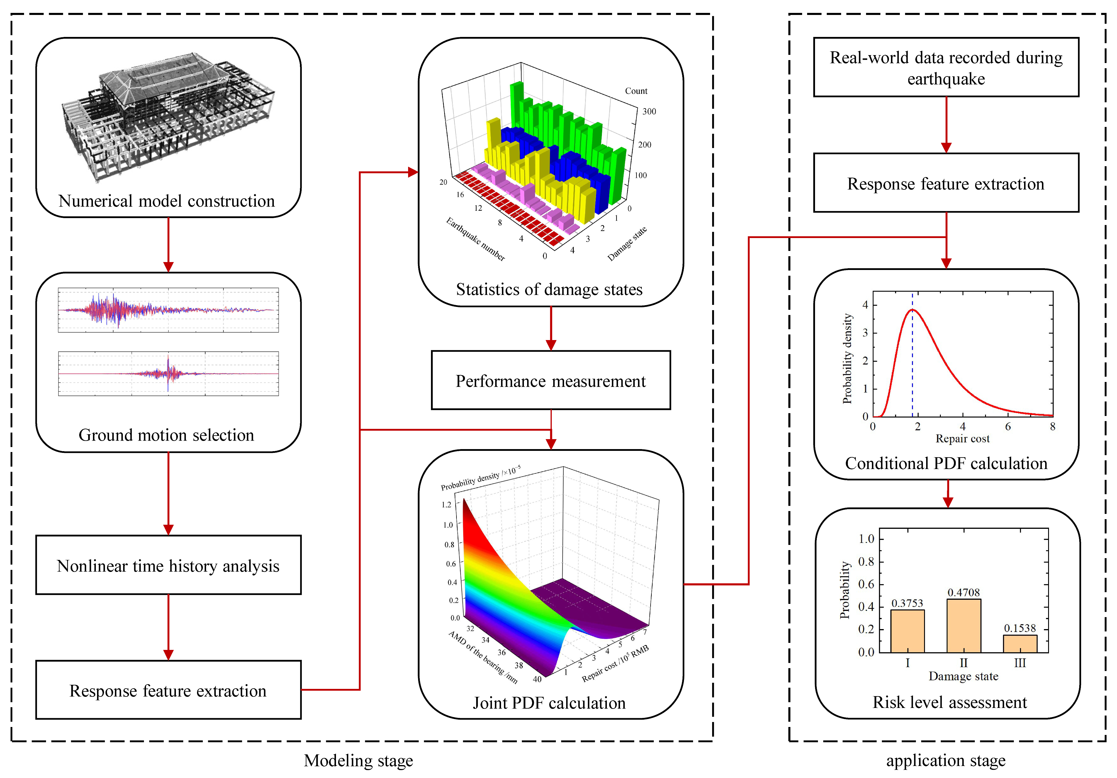
The flow chart of the proposed PBPPA method is illustrated in Figure 1. It can be seen that this method consists of two distinct stages: the modeling stage and the application stage. In the modeling stage, information related to the monitored structure and historical earthquake data is utilized to establish a joint PDF (probability density function) for post-earthquake performance assessment. This joint PDF serves as a fundamental component in capturing the relationship between the seismic response of the structure and its corresponding performance. In the application stage, real-world data recorded during a real earthquake event is input to the established model to calculate the conditional PDF of performance measurement, enabling a probabilistic assessment of the risk level associated with the monitored structure.

During the modeling stage, the proposed PBPPA method comprises seven main steps, as follows:

Step 1: Numerical model construction—A numerical model of the monitored structure is constructed using the finite element analysis (FEA) software OpenSees3.2.2-x64. This model serves as the basis for subsequent analysis to obtain the dynamic response of structural components under the selected ground motions.

Step 2: Ground motion selection—A set of ground motions is selected from a ground motion database. The selected ground motions align with the designed target response spectrum while maintaining a certain level of discreteness. This selection process aims to obtain comprehensive probability information regarding the structural dynamic response. In this study, a greedy-based algorithm [23] is employed to select ground motions that satisfy both the mean and standard deviation of the target response spectrum simultaneously. Additional details of the algorithm can be found in Appendix A. Although the Baker-Lee algorithm was originally developed for conditional-spectrum-based ground-motion selection, it is adopted in this study as a practical record-selection strategy to match the mean and standard deviation of the code-based target response spectra.

Step 3: Nonlinear time-history analysis—Nonlinear time-history analysis is performed to determine the dynamic response of the structure under the selected ground motions.

Step 4: Response feature extraction—Time-domain or frequency-domain features, such as maximum values and dominant frequencies, are extracted from the calculated dynamic response. In this study, the absolute maximum displacement of the selected isolation bearings is used as the response feature for the subsequent probabilistic assessment.

Step 5: Statistics of damage states—Based on the EDPs (engineering demand parameters) calculated through the nonlinear time history analysis, the damage state of each component under each ground motion input is obtained.

Step 6: Calculation of performance measurement—Performance measurements, such as repair cost, repair time, and the number of casualties, are derived from the damage state of each component. The repair cost is adopted as the performance measurement in this study.

Step 7: Calculation of joint PDF—The joint PDF of the performance measurements and dynamic response features is calculated. This step serves as the final stage of the modeling phase and provides the foundation for the subsequent application stage.

During the application stage, the PBPPA method involves three primary steps as follows:

Step 1: Real-world data collection and feature extraction—Real-world dynamic response data during earthquakes is collected in this step. Similar to Step 3 in the modeling stage, relevant features are extracted from the collected data. These features serve as the input for subsequent assessment.

Step 2: Conditional PDF calculation—The joint PDF calculated in the modeling stage is converted into a conditional PDF of performance measurement. This is achieved by leveraging the known features extracted from the real-world data. Based on the conditional probability relationship, the conditional PDF of the performance measurement M given the observed response features F can be calculated from the joint PDF of M and F, as expressed in Equation (1).

$$p\left(M\left|F\right.\right)={\displaystyle \frac{p\left(M,F\right)}{p\left(F\right)}}$$

(1)

Step 3: Risk level assessment—Based on the calculated conditional PDF of the performance measurement, the performance of the structure can be assessed, and the associated probability of the structure being in each risk level (RL_i) given observed features (F) is obtained by integrating the conditional PDF p(M|F) over the range from l_i to u_i, as expressed in Equation (2).

$$R{L}_i\left(F\right)={\displaystyle {\int }_{l_i}^{u_i}p\left(M\left|F\right.\right)dM}$$

(2)

3. Case Study: The Old Hall of Nanjing Museum

3.1. Introduction of the Old Hall of Nanjing Museum

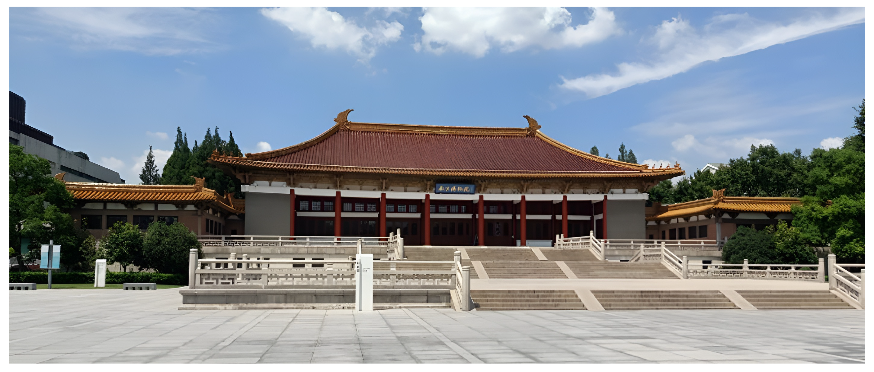
A case study of the Old Hall of Nanjing Museum (Figure 2) is presented in this section to demonstrate the effectiveness and advantages of the proposed PBPPA method. For this case study, both simulated acceleration response data generated through finite element analysis and real-world data collected during an actual earthquake event are utilized.

The Old Hall of Nanjing Museum is the first national large-scale comprehensive museum built in China. It has a rich history spanning 70 years and houses a collection of more than 400,000 invaluable historical relics. While it serves as an important carrier of special historical and cultural significance, the Old Hall of Nanjing Museum itself can be seen as a cultural relic as well. Therefore, the condition evaluation and maintenance of the Old Hall of Nanjing Museum after earthquakes hold immense importance and value.

In recent years, the Old Hall of Nanjing Museum has been retrofitted with base isolation. As part of this retrofitting, the original column in the basement was cut off and the main structure was uplifted by 3 m. Then, a total of 37 LRBs (lead-rubber bearing) and 26 RBs (rubber bearing), each with a diameter of 500 mm, along with 98 RBs with a diameter of 400 mm, were installed between the main structure and the foundation. The application of the base-isolation technique has significantly enhanced the seismic safety of the Old Hall of Nanjing Museum. However, it is important to acknowledge that despite the utilization of advanced construction technologies and high-quality materials during the initial construction of the Old Hall of Nanjing Museum, nearly a century of service and factors such as temperature fluctuations and aging processes make it necessary to closely monitor the structure’s operational condition. Hence, an SHM system has been designed and implemented for the Old Hall of Nanjing Museum in recent years.

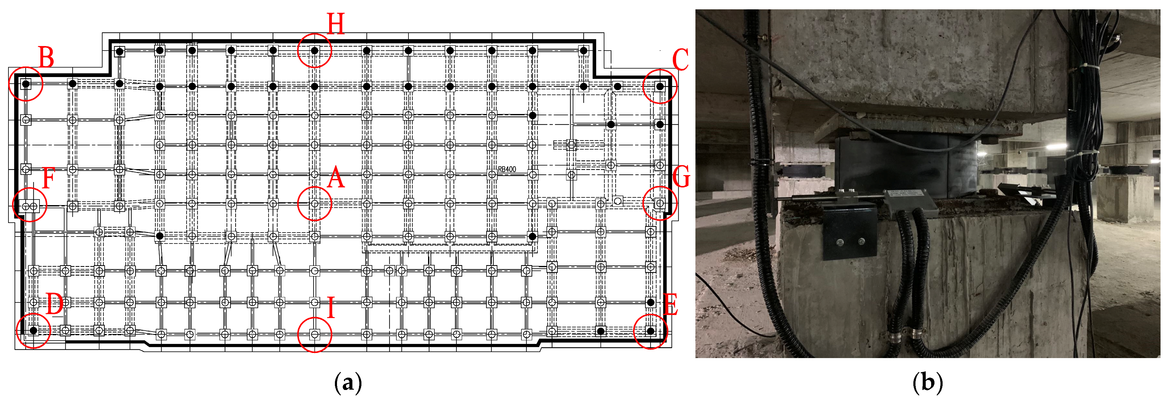
The base-isolation bearings are crucial components in isolated buildings as their operational conditions directly influence the seismic performance of the structure. Considering the structural form and stress characteristics of the Old Hall of Nanjing Museum, a deployment of 76 sensors has been strategically implemented at critical locations within the isolation layer by our group. These sensors are instrumental in capturing real-time structural responses and environmental information, facilitating a comprehensive understanding of the building’s behavior. The types of sensors include fiber-optic thermometers, fiber-optic displacement meters, fiber-optic strain gauges, fiber-optic accelerometers, type-941B vibration sensors, and video displacement sensors. The distribution and arrangement of the isolation bearings and sensors is shown in Figure 3. The five instrumented bearing positions A–E were selected because they are distributed at representative locations of the isolation layer and can reflect both the overall displacement response and possible non-uniform response caused by torsional or eccentric effects. These selected positions therefore provide physically interpretable monitoring features for establishing the probabilistic relationship between bearing displacement responses and repair-cost consequences.

3.2. The Construction of the Numerical Model

For post-earthquake performance analysis, a numerical model is constructed for the Old Hall of Nanjing Museum using the widely adopted open-source software OpenSees3.2.2-x64 (Open System for Earthquake Engineering Simulation). The structural components of the Old Hall of Nanjing Museum include the reinforced concrete beams and columns, steel braces, and isolation bearings. In the modeling process, the flexural members of the structure, namely the beams and columns, are characterized using the “nonlinearBeamColumn” elements. The concrete material is represented by the “Concrete06” material model, while the steel bars are modeled using the “Steel01” material model. These elements and material models effectively capture the nonlinear behavior of the flexural members under seismic loading. The steel braces, which mainly act as axially loaded members in the structure, are simulated using truss elements to represent their axial force-deformation behavior in the global structural model. This simplified treatment is adopted for the purpose of global response analysis and post-earthquake risk assessment. It should be noted that local compression buckling and cyclic strength degradation of steel braces are not explicitly modeled in this study. The isolation bearings are simulated by the “zeroLength” element. The key parameters of the isolation bearings used in the numerical model are summarized in

Table 1. Key parameters of the isolation bearings.

Parameter	LRB500	RB500	RB400
Diameter (mm)	500	500	400
Lead core diameter (mm)	100	/	/
Total rubber layer thickness (mm)	96	100	100
Vertical stiffness (kN/mm)	1728	1237	592
Equivalent horizontal stiffness (kN/mm)	1.428	0.755	0.485
Pre-yield stiffness (kN/mm)	10.075	/	/
Post-yield stiffness (kN/mm)	0.775	/	/
Yield force (kN)	62.6	/	/
Rubber shear modulus (N/mm2)	0.392	0.392	0.392

. To gain insights into the dynamic characteristics of the base-isolated museum, the first three modal shapes of the structure are calculated and illustrated in Figure 4. Since the dynamic characteristics of the base-isolated structure depend on the deformation level of the isolation bearings, the modal periods were compared under different bearing-deformation states. As shown in

Table 2. Comparison of measured and calculated modal periods under different bearing-deformation states.

Mode	Direction	Measured Period Under Small Vibration (s)	Calculated Period Under Initial Stiffness (s)	Difference	Calculated Period Under 100% Shear Strain (s)
1	Horizontal	1.011	1.002	−0.89%	1.801
2	Horizontal	0.964	0.990	2.70%	1.782
3	Torsional	0.968	0.961	−0.72%	1.722

, the measured periods identified from small vibrations are close to the calculated periods based on the initial stiffness, with differences within 3%. In contrast, the calculated periods under the 100% shear strain are much longer, indicating stiffness degradation and period elongation of the isolation system under larger deformation.

3.3. The Selection of Earthquake Waves

According to the Seismic Ground Motion Parameters Zonation Map of China (GB18306-2015) [24], the seismic precautionary intensity of the area where the museum is located is 7, with a design basic earthquake acceleration of 0.10 g. The design earthquake group is group I, with a site category of class II, and the design characteristic period of ground motion in this area is 0.35 s. The seismic fortification category is class C. 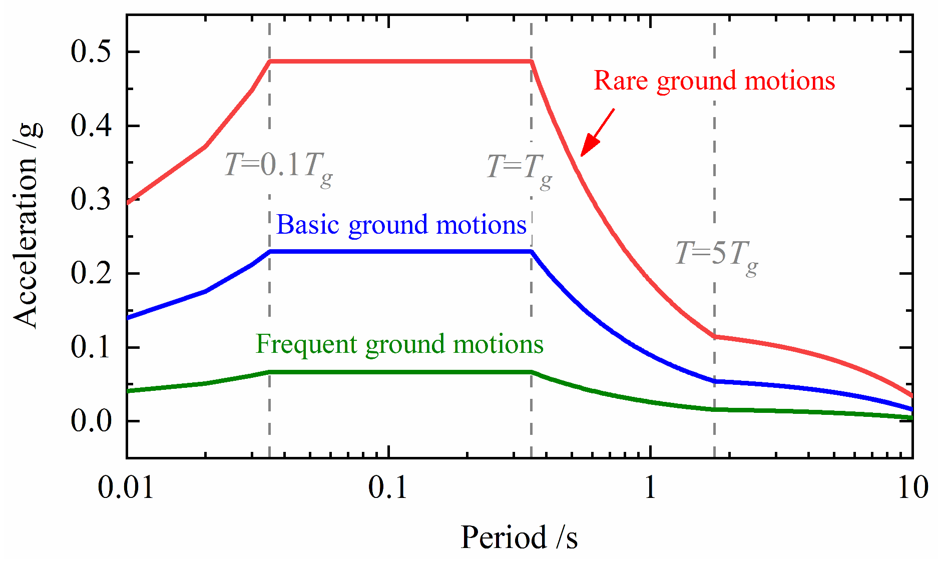Therefore, according to the Code for Seismic Design of Buildings [25], the maximum horizontal earthquake impact coefficients in this region under frequent, basic and rare ground motions are 0.0667, 0.23 and 0.4867. The corresponding probabilities of exceedance within 50 years are 63%, 10% and 2~3%. Three acceleration response spectra for earthquake wave selection are generated for frequent, basic, and rare ground motions, which serve as the target acceleration response spectra for earthquake wave selection, as shown in Figure 5.

The NGA-West2 established by PEER (Pacific Earthquake Engineering Research Center) is used as the database for earthquake wave selection. Using the target spectra described above, 20 earthquake waves are selected from the NGA-West2 for the basic and rare ground motions; therefore, the total number of earthquake waves is 40. The selected earthquake waves and their RSNs (record sequence number) are listed in

Table 3. Selected earthquake waves.

No.	Basic Ground Motions		Rare Ground Motions		No.	Basic Ground Motions		Rare Ground Motions
	RSN	Scaling Factor	RSN	Scaling Factor		RSN	Scaling Factor	RSN	Scaling Factor
1	172	0.70	172	1.49	11	1524	0.47	1485	0.87
2	855	1.37	879	0.59	12	1531	0.48	1487	0.78
3	1148	0.84	1118	1.36	13	1612	1.72	1488	0.81
4	1161	0.46	1148	1.78	14	1786	1.87	1499	1.03
5	1196	1.02	1161	0.98	15	1812	1.79	1510	0.55
6	1239	0.97	1228	1.42	16	2113	1.35	1524	1.00
7	1303	1.55	1350	1.93	17	2115	1.14	1528	0.66
8	1347	1.06	1402	1.39	18	2502	1.97	1531	1.01
9	1476	0.47	1476	0.99	19	3302	0.72	1826	1.91
10	1499	0.49	1483	0.89	20	3312	1.66	3302	1.53

. Detailed metadata such as earthquake magnitude, source-to-site distance, site condition, fault mechanism, and duration characteristics can be retrieved from the PEER database using the RSNs listed in the table.

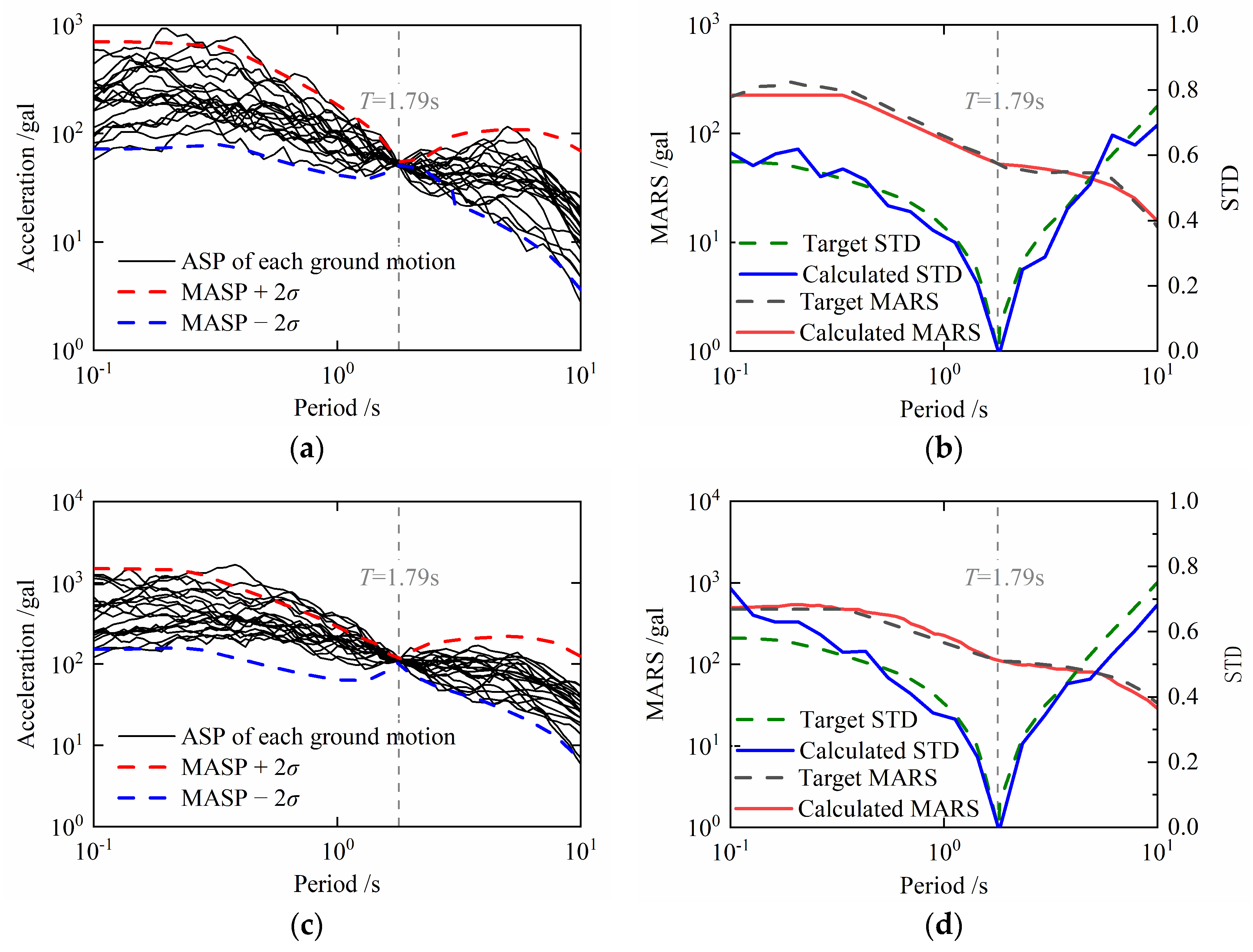
Individual and mean response spectra of the selected basic and rare ground motions are presented in Figure 6a,c. For verification, the mean and standard deviation of the spectra of the selected basic and rare ground motions are presented in Figure 6b,d, compared to the target spectrum and standard deviation. It can be found that the selected records provide an acceptable overall match to the target mean spectrum and capture the dispersion characteristics over the considered period. The response spectrum of the selected ground motions exactly matches the target response spectrum when the period equals 1.79 s, which is the mean value of the first two horizontal modal periods. This ensures obtaining full information on the probability of the structural response.

3.4. Statistics of the Damage States

When the museum is excited by the selected ground motions, EDPs (engineering demand parameters) can be calculated by nonlinear time-history analysis using OpenSees. According to the Standard for Seismic Resilience Assessment of Buildings (GB/T 38591-2020) [26], the damage states of the structural components can be inferred by EDPs. For flexural members like RC (reinforced concrete) beams and columns with normal section failure modes, the damage states are determined based on the principal tensile strain of the concrete and the principal compressive strain of the steel bars. The criteria for the determination of damage states from level 0 to 4 are presented in

Table 4. Damage state determination criteria for reinforced concrete beams and columns with normal section failure modes.

Damage State	Criteria
	Concrete	Steel Bar
Level 0	|εc| ≤ |εp|	And εs ≤ εy
Level 1	|εc| ≤ |εp|	And εy < εs ≤ 2εy
Level 2	|εp| < |εc| ≤ 1.5|εp|	Or 2εy < εs ≤ 3.5εy
Level 3	1.5|εp| < |εc| ≤ |εcu|	Or 3.5εy < εs ≤ 12εy
Level 4	|εc| > |εcu|	Or εs > 12εy

, where ε_c and ε_s stand for the principal tensile strain of the concrete and the principal compressive strain of the steel bars, respectively; ε_p and ε_cu are the peak and ultimate strain of concrete under uniaxial compression, respectively; ε_y is the tensile yield strain of steel bars.

Steel braces are axially loaded members, which means that they can either be in compression or tension. Therefore, the damage state of the steel bars is determined based on the compressive or tensile displacement, as presented in

Table 5. Damage state determination criteria for steel brace.

Damage State	Level 0	Level 1	Level 2	Level 3	Level 4
Criteria	Δ ≤ Δy	Δy < Δ ≤ ΔIO	ΔIO < Δ ≤ ΔLS	ΔLS < Δ ≤ Δu	Δ > Δu

, where Δ_y, Δ_IO, Δ_LS and Δ_u are the yield displacement, IO (immediate occupation) displacement, LS (life safety) displacement and ultimate displacement, respectively.

For steel braces with H-shaped and I-shaped sections, the three control points Δ_IO, Δ_LS and Δ_u can be determined by multiplying Δ_y by a coefficient, as presented in

Table 6. The determination criteria for Δ_IO, Δ_LS and Δ_u.

Stress Condition	ΔIO/Δy	ΔLS/Δy	Δu/Δy
In Tension	1.5	11	14
Compressed and ${\displaystyle \frac{Kl}{i}}\ge 4.2\sqrt{{\displaystyle \frac{E}{F_y}}}$	1.5	9	11
Compressed and ${\displaystyle \frac{Kl}{i}}\le 2.1\sqrt{{\displaystyle \frac{E}{F_y}}}$	1.5	8	9
Compressed and $2.1\sqrt{{\displaystyle \frac{E}{F_y}}}\le {\displaystyle \frac{Kl}{i}}\le 4.2\sqrt{{\displaystyle \frac{E}{F_y}}}$	Linear interpolation

, where K is the effective length factor; l is the length of the steel brace; i is the radius of gyration; E is the elastic modulus; and F_y is the yield strength of the steel. The displacement limits corresponding to different damage states are determined according to the slenderness-ratio range. When the slenderness ratio of a brace falls between two tabulated boundary values, the corresponding displacement limit is obtained by linear interpolation between the two boundary values.

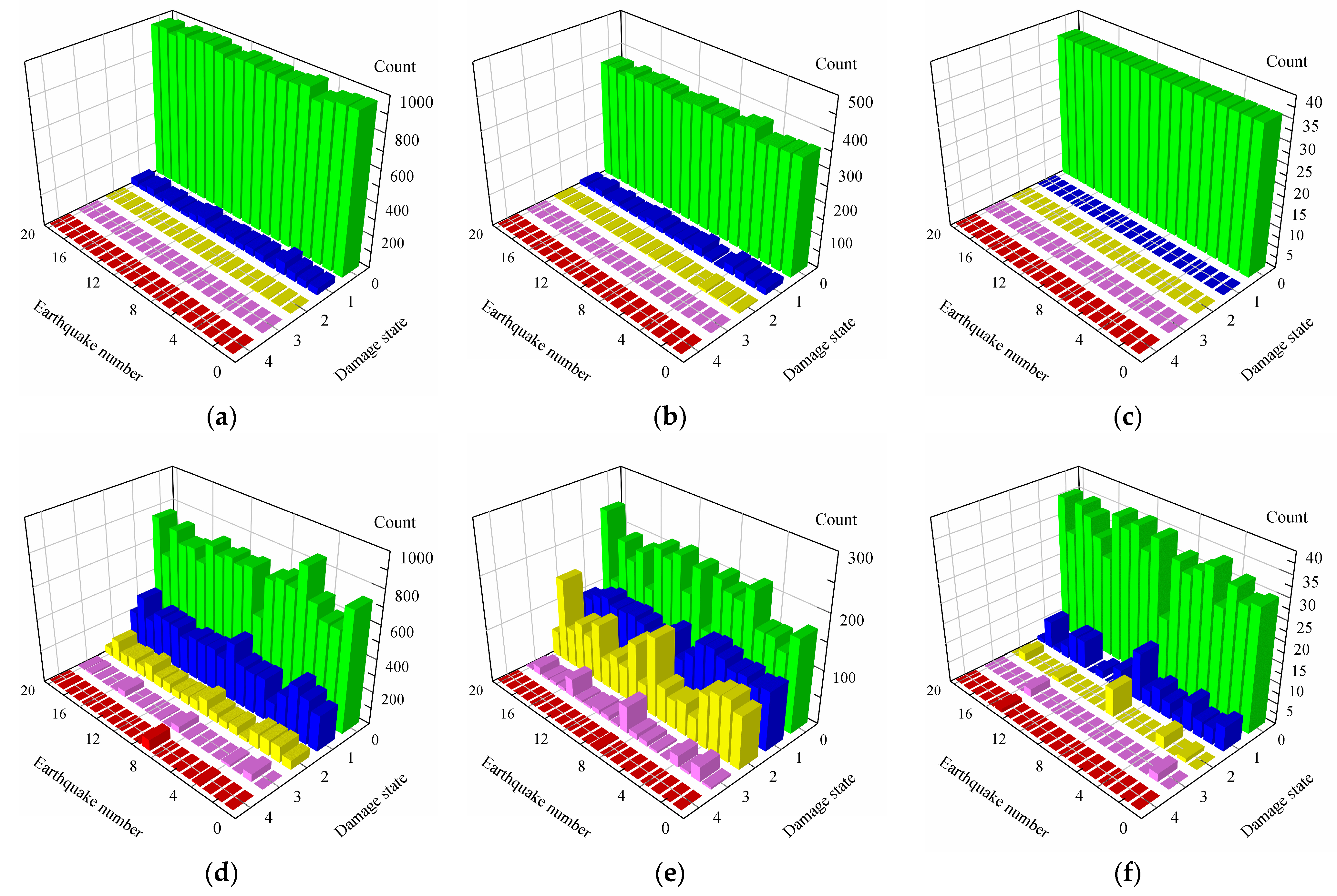
According to the damage state determination criteria presented above, the damage states of RC beams, columns and steel braces corresponding to each basic and rare ground motion input are counted respectively, as shown in Figure 7. It can be seen that under the basic ground motions, an extremely small number of beams and columns are in the level 1 damage state. It can also be found that all braces are in the level 0 damaged state, namely undamaged. Under the rare ground motions, beams, columns, and braces all suffer damage to a certain extent, but the percentage of beams and braces in the level 0~1 damage state is relatively large, while the percentage of columns in the level 2 damage state is slightly larger. This is mainly because the structural height-to-width ratio of the museum is low and the plane layout is symmetrical; therefore, the floor deformation is mainly caused by shear deformation, resulting in a smaller deformation of beams than columns. Meanwhile, owing to the seismic isolation effect of the isolation bearings, the seismic demand transmitted to the superstructure is significantly reduced. Therefore, even under rare ground motions, most column damage states are controlled at Level 2 or below.

3.5. Statistics of the Performance Measures

According to the FEMA-P58 [27], “a seismic performance measure is defined as a means of quantifying the consequences associated with the response of a building to earthquake shaking in terms that are intended to be meaningful to decision-makers”. Repair cost is one of the performance measures important to decision-makers, defined as the cost necessary to restore a building to its pre-earthquake condition, or in the case of total loss, to replace the building with a new structure of similar condition.

The repair loss is used in this case study to assess the post-earthquake condition of the museum. According to GB/T 38591-2020 [26], the repair loss can be calculated using Equation (3).

$$\begin{array}{cc}{R}_T& ={\displaystyle \sum _{n=1}^3{\displaystyle \sum _{k=1}^4{\lambda }_{C\left(k\right)}{R}_{\left(n,k\right)}}}\hfill \\ & ={\displaystyle \sum _{n=1}^3\left\{{\zeta }_{C\left(n\right)}{\displaystyle \sum _{j=0}^4\left[{\displaystyle \sum _{k=1}^4{\lambda }_{C\left(k\right)}\left({\eta }_{1\left(n,j\right)}\times L_{\left(n,j,k\right)}\right)}\right]}\right\}}\end{array}$$

(3)

where

$$L_{\left(n,j,k\right)}={\eta }_{2\left(n,j\right)}\times C_{\left(n,j,k\right)}$$

(4)

In the above equations, n denotes the type of the structural components, namely RC beams, columns, steel braces; k denotes the floor where the structural components are located; λ_C(k) is the coefficient of repair cost for each floor, reflecting the difficulty of repairing the damaged components considering the floor position; R_(n,k) is the repair cost for the components of type n on the k-th floor; ζ_C(n) is the reduction coefficient of the repair cost for the type n components, reflecting the reduction on unit repair cost with the increase in repair quantity; j denotes the damage state; L_(n,j,k) is the economic loss of the type n components of damage state j in the k-th floor, which can be calculated by Equation (4); η_1(n,j) is the ratio of repair cost to the economic loss for the type n components of damage state j; C_(n,j,k) is the total construction cost of the type n components of damage state j in the k-th floor; η_2(n,j) is the ratio of economic loss to the construction cost for the type n component of damage j in the k-th floor. The unit construction costs for RC beams, columns and steel braces used in this article are 645.91 RMB/m³, 1371.59 RMB/m³, and 5818.83 RMB/t. The values of λ_C(k), ζ_C(n), η_1(n,j), and η_2(n,j) were determined according to the recommended coefficient values in GB/T 38591-2020 [26].

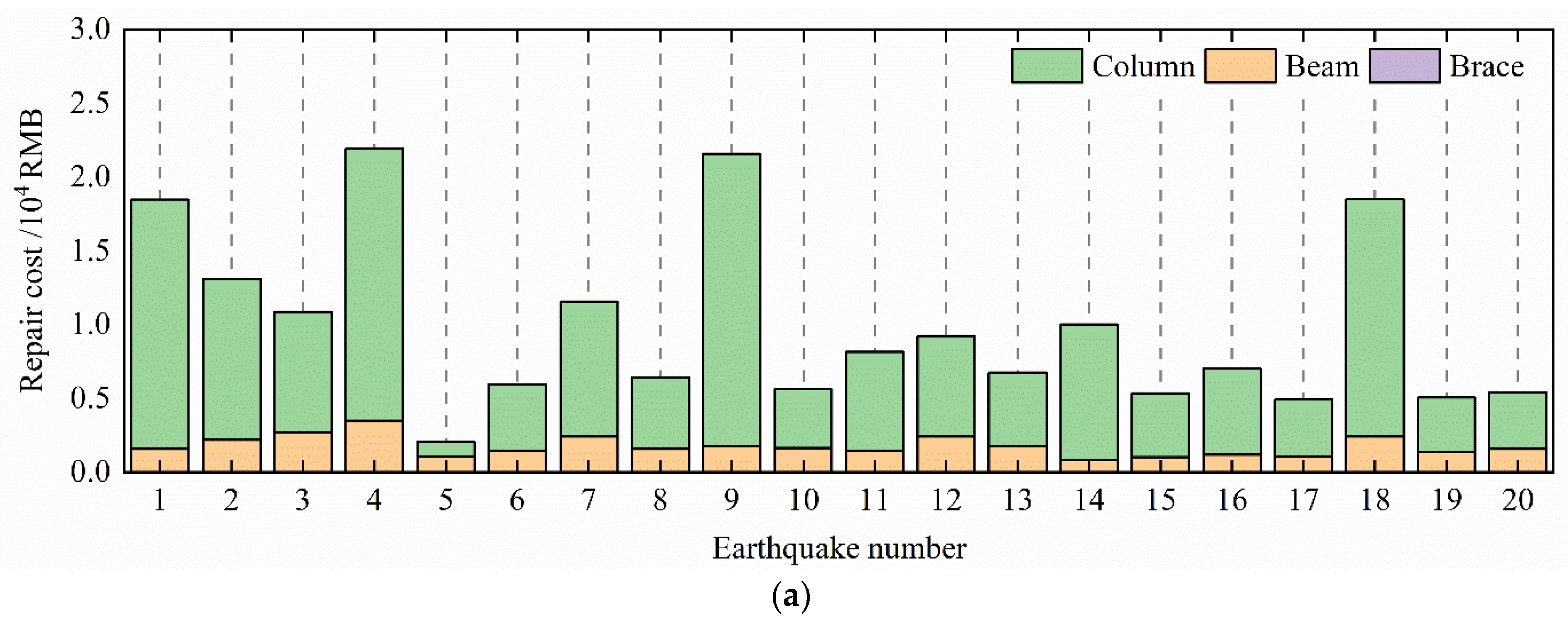
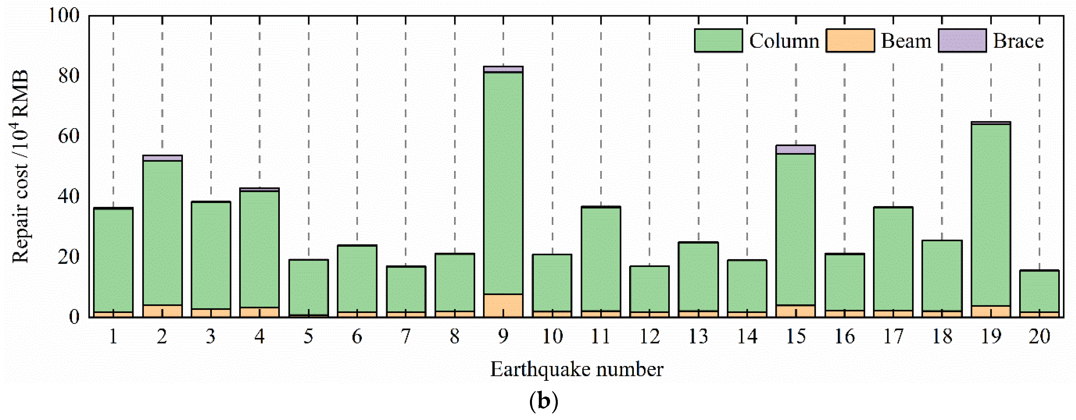
Based on the assessment result of component damage state in Figure 7, the repair cost of the Old Hall of Nanjing Museum under basic and rare ground motions is calculated using Equation (3). As can be seen in Figure 8, the repair cost of columns accounts for the largest proportion, while the repair cost of steel braces accounts for the minimum proportion.

3.6. Probabilistic Estimation of the Post-Earthquake Performance Measures

The dynamic response collected by sensors cannot directly reflect the post-earthquake working condition and the corresponding repair cost of the structure. However, there is a correlation between the collected dynamic response and performance measurements. The proposed PBPPA is designed to recognize and quantify this relationship, and then assess the post-earthquake working condition of the structure.

For verification, the correlation coefficients between the absolute maximum displacement (AMD) of isolation bearings at selected positions and the repair cost of the museum are presented in

Table 7. Correlation coefficients between the AMD of isolation bearings and the repair cost of the museum.

	Position A	Position B	Position C	Position D	Position E	Repair Cost
Position A	1.00	0.87	0.89	0.85	0.78	0.90
Position B	0.87	1.00	0.93	0.82	0.89	0.92
Position C	0.89	0.93	1.00	0.88	0.89	0.94
Position D	0.85	0.82	0.88	1.00	0.91	0.85
Position E	0.78	0.89	0.89	0.91	1.00	0.83
Repair cost	0.90	0.92	0.94	0.85	0.83	1.00

. It can be found that the correlation coefficients are all larger than 0.8, indicating that the AMD and the repair cost are highly correlated. Therefore, the probability distribution function of repair cost can be calculated by the AMD of the selected isolation bearings collected during earthquakes.

Since the selected EDPs and performance measurements, such as bearing displacement and repair cost, are non-negative and usually exhibit right-skewed probabilistic characteristics under earthquake excitations, the lognormal distribution is adopted to describe their uncertainty. This assumption is also consistent with the probabilistic modeling framework recommended in FEMA-P58 [27] and GB/T 38591-2020 [26]. This assumption allows the relationship between monitored EDPs and repair cost consequences to be characterized using a limited number of numerical simulations, thereby reducing the number of required nonlinear time history analyses. Therefore, the EDPs and performance measurements are assumed to follow a multidimensional lognormal distribution. Equivalently, their logarithmic values are assumed to follow a multidimensional normal distribution, as described in Equation (5). For the base-isolated Old Hall of Nanjing Museum, the displacement response of the isolation bearings is selected as the primary feature EDP because it directly represents the deformation demand of the isolation layer during an earthquake. The maximum displacement of the isolation bearings has a clear physical relationship with the seismic performance of the isolation system and the potential damage consequences of the structure.

$$p\left(X_r,X_u\right)={\displaystyle \frac{1}{{\left(2\pi \right)}^3{|\mathsf{\Sigma }|}^{\frac{1}{2}}}}\exp \left[-{\displaystyle \frac{1}{2}}{\left(X-\mu \right)}^T{\mathsf{\Sigma }}^{-1}\left(X-\mu \right)\right]$$

(5)

where X_r is the logarithmic repair cost under the selected basic and rare ground motions; X_u = (ln(U_max,_A), ln(U_max,_B), ln(U_max,C), ln(U_max,D), ln(U_max,E)) is a 5-dimensional vector of the maximum logarithmic displacement of five selected isolation bearings; X = (X_r, X_u) is a 6-dimensional vector; μ is a 6-dimensional mean value vector of the random variable vector X; Σ is a 6-by-6-dimensional covariance matrix of the random variable vector X. The unknown μ and Σ can be estimated based on the simulated 40 samples of the AMD of isolation bearings and the repair cost under basic and rare ground motions.

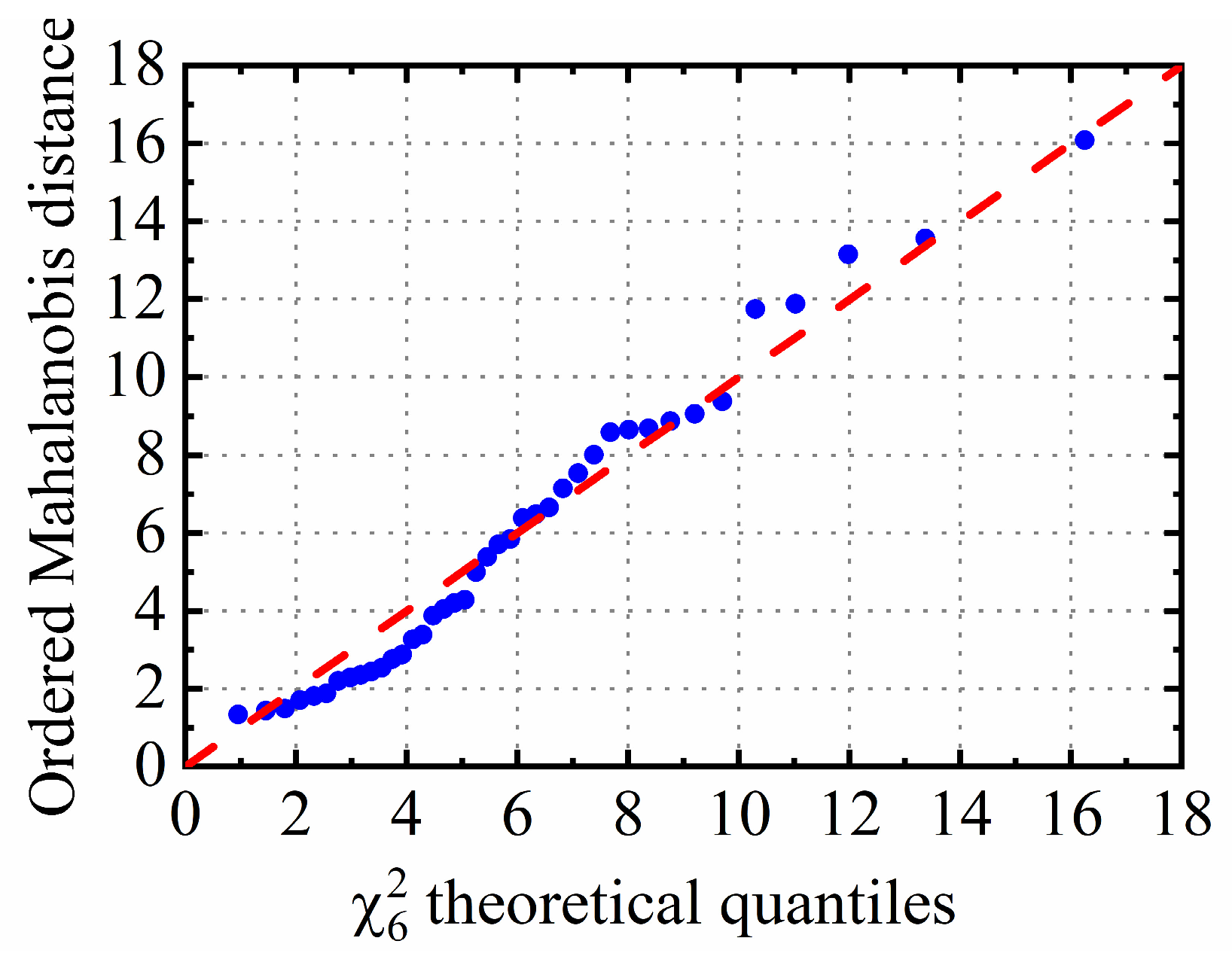
To further examine the multidimensional lognormal assumption, a Mahalanobis distance Q-Q plot is used to check the multivariate normality of the logarithmic variables. If the six-dimensional logarithmic vector X approximately follows a multivariate normal distribution with mean vector μ and covariance matrix Σ, the squared Mahalanobis distance of the i-th sample $D_i^2={(X_i- \mu )}^T {\mathsf{\Sigma }}^{-1}(X_i-\mu )$ approximately follows a chi-square distribution with six degrees of freedom. The linearity of the Mahalanobis distance Q-Q plot provides a graphical check of the multivariate normality assumption. As shown in Figure 9, the ordered squared Mahalanobis distances are approximately aligned with the theoretical χ²(6) quantiles, indicating that the logarithmic repair cost and bearing displacement vector can be reasonably approximated by a six-dimensional normal distribution in the present case study. This result supports the use of the multidimensional lognormal model in Equation (5).

When the joint probability function p(X_r,X_u) is a multi-dimensional normal distribution, the conditional PDF p(X_r|X_u) is also a normal distribution. The mean value μ_c and covariance matrix Σ_c of p(X_r|X_u) are calculated by Equation (6).

$$\begin{array}{l}{\mu }_c={\mu }_r+{\mathsf{\Sigma }}_{ru}{\mathsf{\Sigma }}_{uu}^{-1}\left(X_u-{\mu }_u\right)\\ {\mathsf{\Sigma }}_c={\mathsf{\Sigma }}_{rr}-{\mathsf{\Sigma }}_{ru}{\mathsf{\Sigma }}_{uu}^{-1}{\mathsf{\Sigma }}_{ur}\end{array}$$

(6)

where μ_r and μ_u are the mean values of X_r and X_u respectively; Σ_rr, Σ_ru, Σ_ur, Σ_uu are the submatrices of Σ, as described in Equation (7). Accordingly, Σ_uu is a 5 × 5 covariance matrix, Σ_rr is a 1 × 1 variance term, Σ_ru is a 1 × 5 cross-covariance matrix, and Σ_ur is a 5 × 1 cross-covariance matrix.

$$\mathsf{\Sigma }=\left[\begin{array}{cc}{\mathsf{\Sigma }}_{rr}& {\mathsf{\Sigma }}_{ru}\\ {\mathsf{\Sigma }}_{ur}& {\mathsf{\Sigma }}_{uu}\end{array}\right]=\left[\begin{array}{cccccc}{\mathsf{\Sigma }}_{11}& {\mathsf{\Sigma }}_{12}& {\mathsf{\Sigma }}_{13}& {\mathsf{\Sigma }}_{14}& {\mathsf{\Sigma }}_{15}& {\mathsf{\Sigma }}_{16}\\ {\mathsf{\Sigma }}_{21}& {\mathsf{\Sigma }}_{22}& {\mathsf{\Sigma }}_{23}& {\mathsf{\Sigma }}_{24}& {\mathsf{\Sigma }}_{25}& {\mathsf{\Sigma }}_{26}\\ {\mathsf{\Sigma }}_{31}& {\mathsf{\Sigma }}_{32}& {\mathsf{\Sigma }}_{33}& {\mathsf{\Sigma }}_{34}& {\mathsf{\Sigma }}_{35}& {\mathsf{\Sigma }}_{36}\\ {\mathsf{\Sigma }}_{41}& {\mathsf{\Sigma }}_{42}& {\mathsf{\Sigma }}_{43}& {\mathsf{\Sigma }}_{44}& {\mathsf{\Sigma }}_{45}& {\mathsf{\Sigma }}_{46}\\ {\mathsf{\Sigma }}_{51}& {\mathsf{\Sigma }}_{52}& {\mathsf{\Sigma }}_{53}& {\mathsf{\Sigma }}_{54}& {\mathsf{\Sigma }}_{55}& {\mathsf{\Sigma }}_{56}\\ {\mathsf{\Sigma }}_{61}& {\mathsf{\Sigma }}_{62}& {\mathsf{\Sigma }}_{63}& {\mathsf{\Sigma }}_{64}& {\mathsf{\Sigma }}_{65}& {\mathsf{\Sigma }}_{66}\end{array}\right]$$

(7)

where Σ_ij represents the i-th row and j-th column element of the covariance matrix Σ. Hence, the conditional PDF p(X_r|X_u) is calculated by Equation (8).

$$p\left(X_r\left|X_u\right.\right)={\displaystyle \frac{1}{{\left(2\pi \right)}^{\frac{1}{2}}{\left|{\mathbf{\Sigma }}_c\right|}^{\frac{1}{2}}}}\exp \left\{-{\displaystyle \frac{1}{2}}{\left(X_r-{\mu }_c\right)}^T{\mathbf{\Sigma }}_c^{-1}\left(X_r-{\mu }_c\right)\right\}$$

(8)

Therefore, for the repair cost Y_r = exp(X_r) and the AMD of base-isolation bearings Y_u = exp(X_u), the conditional PDF p(Y_r|Y_u) is a lognormal distribution as described in Equation (9).

$$p\left(Y_r\left|Y_u\right.\right)={\displaystyle \frac{1}{{\left(2\pi \right)}^{\frac{1}{2}}{Y}_r{\left|{\mathbf{\Sigma }}_c\right|}^{\frac{1}{2}}}}\exp \left\{-{\displaystyle \frac{1}{2}}{\left(\ln Y_r-{\mu }_c\right)}^T{\mathbf{\Sigma }}_c^{-1}\left(\ln Y_r-{\mu }_c\right)\right\}$$

(9)

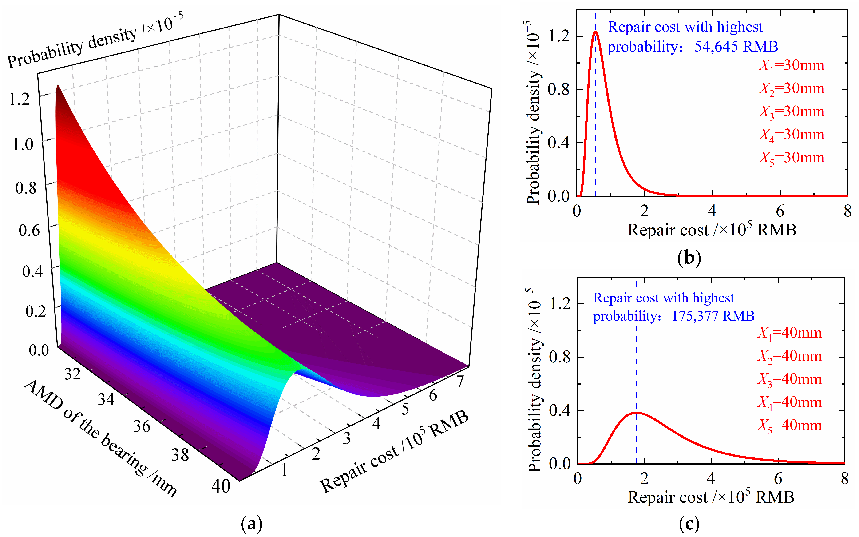
For illustration, the displacement of the monitored isolation bearings in Figure 9 is set to be identical. Using Equation (9), the joint PDF and conditional PDF of the repair cost can be obtained. It should be noted that the identical AMDs assigned to the five selected isolation bearings are used only for visualization and parametric illustration. This setting allows the influence of response amplitude on the conditional repair-cost distribution and risk-level probabilities to be presented more clearly. In actual earthquake events, the displacement responses of different isolation bearings may be non-uniform due to torsional or eccentric effects. In the real-world application of the Jiangning earthquake in Section 3.8, the AMDs of the selected bearings are directly obtained from the measured monitoring data, and the five input displacement values are not identical.

In Figure 10, it can be seen that the mean and standard deviation of the conditional PDF of the repair cost are positively correlated with the AMD of isolation bearings. When the AMD of all the isolation bearings equals 30 mm, the most probable repair cost is 54,645 RMB. When the AMD of all the isolation bearings equals 40 mm, the most probable repair cost is 175,377 RMB, and the deviation is obviously higher. This indicates that a higher repair cost may result if the AMD of isolation bearings is higher, and the repair cost is more difficult to predict. This can be interpreted by the fact that when the earthquake magnitude is small, the structural response is linear; therefore, the most probable repair cost is low and easy to predict.

3.7. Risk Level Assessment

The PDF of repair cost can reflect the post-earthquake performance of the structure to some extent; however, to accurately reflect the health condition of the structure, the repair cost should be further compared with the total construction cost. Based on the repair-cost ratio criterion described in the GB/T 38591-2020 [26], a three-level risk rating criterion is established, as presented in Equations (10)–(12).

$$p\left(\mathrm{risk} \mathrm{level}= I\right)={\displaystyle {\int }_0^{5\% \mathrm{construnction} \mathrm{cost}}p\left(Y_r\left|Y_u\right.\right)}d{Y}_r$$

(10)

$$p\left(\mathrm{risk} \mathrm{level}= II\right)={\displaystyle {\int }_{5\% \mathrm{construnction} \mathrm{cost}}^{10\% \mathrm{construnction} \mathrm{cost}}p\left(Y_r\left|Y_u\right.\right)}d{Y}_r$$

(11)

$$p\left(\mathrm{risk} \mathrm{level}= III\right)={\displaystyle {\int }_{10\% \mathrm{construnction} \mathrm{cost}}^{\infty }p\left(Y_r\left|Y_u\right.\right)}d{Y}_r$$

(12)

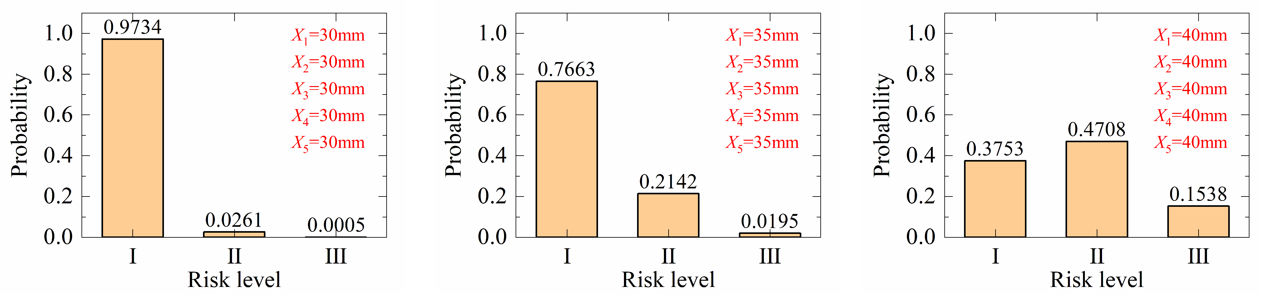
When the AMD of all the base-isolation bearings is equal to 30 mm, 35 mm, and 40 mm, respectively, the probabilities of the museum being in each risk level are calculated and presented in Figure 11. As shown, when the AMDs of all the base-isolation bearings are equal to 30 mm, the probability of the museum being in risk level I is significantly higher than in risk levels II and III, indicating that the museum remains intact. When the AMD of the selected isolation bearings is 35 mm, the probability of risk level I decreases to 0.7663, while the probability of risk level II increases to 0.2142. Although risk level I remains the most probable assessment result, the increase in the probability of risk level II indicates that the post-earthquake risk becomes more significant as the bearing displacement increases. When the AMDs of all the base-isolation bearings are equal to 40 mm, the probability of being in risk level II is among the highest and the probability of being in risk level III increases significantly, indicating that further inspections are necessary.

3.8. Real-World Application of the Proposed PBPPA

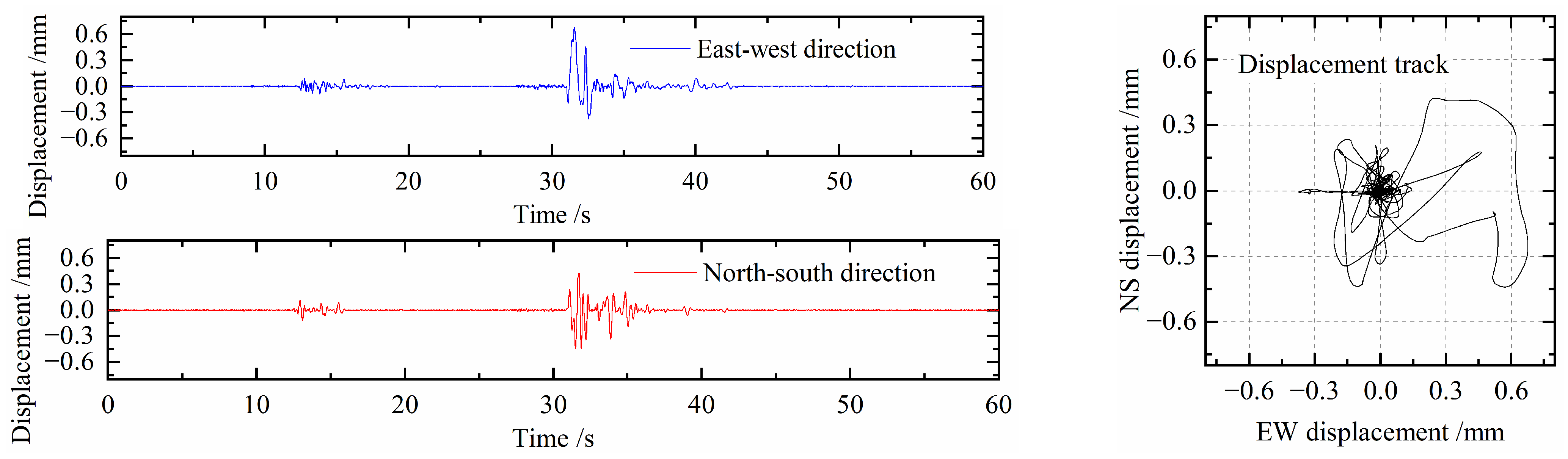
On 25 December 2020, an earthquake with magnitude 2.7 struck Jiangning District, Nanjing, where the Old Hall of Nanjing Museum is located. Although the earthquake magnitude was low, the vibration was felt in many areas of Nanjing. The health monitoring system of the Old Hall of Nanjing Museum successfully recorded the dynamic response of the base-isolation bearings during the earthquake. After denoising using the wavelet transform, the displacement histories of the center isolation bearing in both directions are shown in Figure 12.

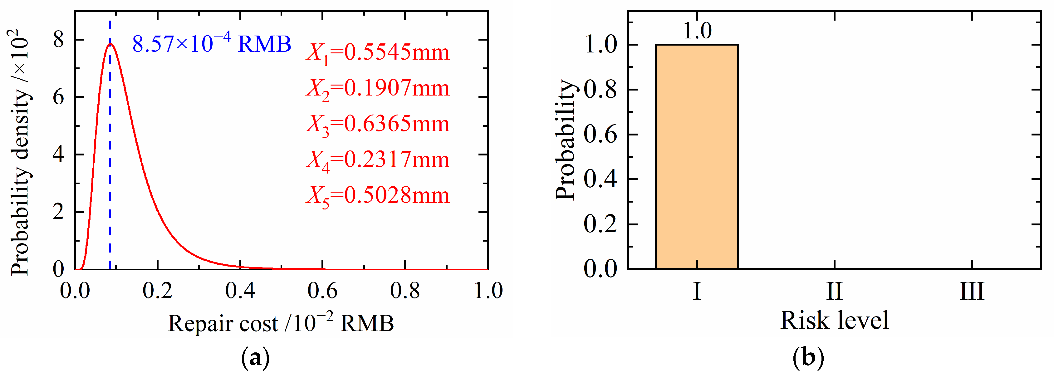
Replace the AMD of base-isolation bearings in Equation (9)–(12) with data recorded during the Jiangning earthquake; the conditional PDF of the repair cost and the result of risk level assessment are presented in Figure 13. As can be seen, the repair cost corresponding to the maximum value of the conditional PDF is extremely low, and the probability of the museum being in risk level I is 100%. Therefore, the museum is considered intact after the Jiangning earthquake, which is consistent with the actual condition. This real-world earthquake case demonstrates that the proposed PBPPA procedure can be implemented using monitoring data collected during an actual seismic event. However, because the Jiangning earthquake was a low-intensity event and the recorded responses were very small, this case mainly verifies that the structure is classified as a low-risk condition under a very low-response state. Further validation using stronger earthquake records, publicly available benchmark datasets, or shake-table experiments will be conducted in future work.

4. Conclusions and Future Work

To ensure prompt assessment of structural damage following earthquakes and ensure structural safety, traditional on-site inspections by technicians have limitations in terms of time consumption and labor intensity. It is also difficult to determine whether inspection and maintenance are needed after an earthquake when the magnitude is low. Moreover, on-site inspections can be easily influenced by the working environment and the working conditions of the technicians, which often leads to misjudgments and omissions. To address these challenges, this paper focuses on the rapid post-earthquake assessment utilizing monitoring data and proposes a performance-based probabilistic post-earthquake assessment (PBPPA) method. The Old Hall of Nanjing Museum is considered a case study, where both simulated data and real-world data collected during an earthquake are used to demonstrate and validate the proposed method. The main findings and conclusions are summarized as follows:

(1)

Through the numerical simulations of the Old Hall of Nanjing Museum, it is observed that when the absolute value of the maximum displacement of the isolation bearings remains below 30 mm, the probability of the structure being in the risk level I reaches 97.34%. As the absolute value of the maximum displacement of the isolation bearings increases to 35 mm and 40 mm, the probability of the structure being in risk level I starts to decrease (76.63% and 37.53%, respectively), and the probability of the risk levels II and III increases. Additionally, it is found that the standard deviation of the probability density function also increases with the absolute value of the maximum displacement of the isolation bearings. This observation is consistent with the fact that nonlinear response leads to an increased variability in dynamic responses. The above verifies that the proposed PBPPA is effective in assessing the post-earthquake risk level through the vibrational data.

(2)

Using the measured data collected during a M 2.7 earthquake in Jiangning District, Nanjing, on 25 December 2020, it is found that the probability of the structure being in risk level I reaches 100%, aligning with the actual condition observed. This demonstrates the applicability of the PBPPA procedure to real-world monitoring data under a low-intensity earthquake event.

The key innovation of this article lies in the proposal of a performance-based probabilistic post-earthquake assessment method called PBPPA, which enables the rapid evaluation of damage conditions and the assessment of associated consequences by leveraging vibration data obtained from earthquake events. Compared with the conventional vibration-based approaches, this method takes into account the inherent randomness of earthquakes and the nonlinear response of structures by deriving the conditional distribution of performance measures from the joint probabilistic model. Another highlight is that this method enables the assessment of performance-related consequences such as repair cost, repair time and casualties, as well as the corresponding risk levels.

As for future work, the following needs to be further studied:

(1)

It should be noted that the 40 numerical samples used in this case study may introduce uncertainty in the estimation of the covariance matrix and the resulting risk-level probabilities. Future studies will further consider Bayesian estimation or surrogate modeling techniques to quantify and reduce this uncertainty.

(2)

The correlation between the measurement and the performance will be better described using Bayesian neural networks. The results obtained in this article will be the baseline for future research.

(3)

The basic and rare ground-motion cases are pooled to establish a joint probabilistic relationship over a wider response range. This treatment allows the conditional repair-cost distribution to be evaluated for different monitored displacement levels. However, the EDP-repair cost relationship may become intensity-dependent under stronger nonlinear responses, and this issue will be further investigated using more ground-motion records in future work.

(4)

More comprehensive verifications utilizing data from larger earthquakes or shake table tests will be carried out.

References

- Farrar, C.R.; Worden, K. An introduction to structural health monitoring. Philos. Trans. R. Soc. A Math. Phys. Eng. Sci. 2007, 365, 303–315. [Google Scholar] [CrossRef] [Scilit] [PubMed]
- Shi, S.; Du, D.; Mercan, O.; Kalkan, E.; Wang, S. A novel unsupervised real-time damage detection method for structural health monitoring using machine learning. Struct. Control Health Monit. 2022, 29, e3042. [Google Scholar] [CrossRef] [Scilit]
- Shi, S.; Du, D.; Mercan, O.; Kalkan, E.; Parol, J. Contrastive and self-supervised learning for open-set damage classification in structural health monitoring with incomplete and imbalanced vibration data. Expert Syst. Appl. 2025, 293, 128731. [Google Scholar] [CrossRef] [Scilit]
- Shi, S.; Du, D.; Mercan, O.; Kalkan, E.; Parol, J. A novel decentralized damage detection method for self-powered wireless sensing in structural health monitoring using self-supervised learning. Eng. Struct. 2025, 344, 121399. [Google Scholar] [CrossRef] [Scilit]
- Sohn, H.; Czarnecki, J.A.; Farrar, C.R. Structural Health Monitoring Using Statistical Process Control. J. Struct. Eng. 2000, 126, 1356–1363. [Google Scholar] [CrossRef] [Scilit]
- Figueiredo, E.; Park, G.; Farrar, C.R.; Worden, K.; Figueiras, J. Machine learning algorithms for damage detection under operational and environmental variability. Struct. Health Monit. 2011, 10, 559–572. [Google Scholar] [CrossRef] [Scilit]
- Eltouny, K.; Gomaa, M.; Liang, X. Unsupervised Learning Methods for Data-Driven Vibration-Based Structural Health Monitoring: A Review. Sensors 2023, 23, 3290. [Google Scholar] [CrossRef] [Scilit] [PubMed]
- Shi, S.; Du, D.; Mercan, O.; Kalkan, E.; Wang, S. A novel data-driven sensor placement optimization method for unsupervised damage detection using noise-assisted neural networks with attention mechanism. Mech. Syst. Signal Process. 2024, 209, 111075. [Google Scholar] [CrossRef] [Scilit]
- Tsuchimoto, K.; Narazaki, Y.; Spencer, B.F. Development and validation of a post-earthquake safety assessment system for high-rise buildings using acceleration measurements. Mathematics 2021, 9, 1758. [Google Scholar] [CrossRef] [Scilit]
- Tsuchimoto, K.; Narazaki, Y.; Hoskere, V.; Spencer, B.F. Rapid postearthquake safety evaluation of buildings using sparse acceleration measurements. Struct. Health Monit. 2021, 20, 1822–1840. [Google Scholar] [CrossRef] [Scilit]
- Ge, X.; Alexander, N.A.; Kashani, M.M. Rapid post-earthquake damage assessment of ageing reinforced concrete bridge piers using time-frequency analysis. Struct. Infrastruct. Eng. 2021, 17, 1228–1244. [Google Scholar] [CrossRef] [Scilit]
- Hu, R.-P.; Xu, Y.-L. SHM-Based Seismic Performance Assessment of High-Rise Buildings under Long-Period Ground Motion. J. Struct. Eng. 2019, 145, 04019038. [Google Scholar] [CrossRef] [Scilit]
- de Lautour, O.R.; Omenzetter, P. Prediction of seismic-induced structural damage using artificial neural networks. Eng. Struct. 2009, 31, 600–606. [Google Scholar] [CrossRef] [Scilit]
- Morfidis, K.; Kostinakis, K. Approaches to the rapid seismic damage prediction of r/c buildings using artificial neural networks. Eng. Struct. 2018, 165, 120–141. [Google Scholar] [CrossRef] [Scilit]
- Liu, W.; Dong, P.; Liu, J.; Guo, H. Evaluation of three-dimensional shape signatures for automated assessment of post-earthquake building damage. Earthq. Spectra 2013, 29, 897–910. [Google Scholar] [CrossRef] [Scilit]
- Ma, H.; Liu, Y.; Ren, Y.; Yu, J. Detection of collapsed buildings in post-earthquake remote sensing images based on the improved YOLOv3. Remote Sens. 2020, 12, 44. [Google Scholar] [CrossRef] [Scilit]
- Zhang, R.; Duan, K.; You, S.; Wang, F.; Tan, S. A novel remote sensing detection method for buildings damaged by earthquake based on multiscale adaptive multiple feature fusion. Geomat. Nat. Hazards Risk 2020, 11, 1912–1938. [Google Scholar] [CrossRef] [Scilit]
- Syifa, M.; Kadavi, P.R.; Lee, C.W. An artificial intelligence application for post-earthquake damage mapping in Palu, central Sulawesi, Indonesia. Sensors 2019, 19, 542. [Google Scholar] [CrossRef] [Scilit] [PubMed]
- Levine, N.M.; Spencer, B.F. Post-Earthquake Building Evaluation Using UAVs: A BIM-Based Digital Twin Framework. Sensors 2022, 22, 873. [Google Scholar] [CrossRef] [Scilit] [PubMed]
- Zhai, W.; Shen, H.; Huang, C.; Pei, W. Building earthquake damage information extraction from a single post-earthquake PolSAR image. Remote Sens. 2016, 8, 171. [Google Scholar] [CrossRef] [Scilit]
- Ierimonti, L.; Cavalagli, N.; Venanzi, I.; García-Macías, E.; Ubertini, F. A Bayesian-based inspection-monitoring data fusion approach for historical buildings and its post-earthquake application to a monumental masonry palace. Bull. Earthq. Eng. 2023, 21, 1139–1172. [Google Scholar] [CrossRef] [Scilit]
- Farrar, C.R.; Beck, J.L. Special issue of earthquake engineering and structural dynamics on earthquake engineering applications of structural health monitoring. Earthq. Eng. Struct. Dyn. 2015, 44, 499–500. [Google Scholar] [CrossRef] [Scilit]
- Baker, J.W.; Lee, C. An Improved Algorithm for Selecting Ground Motions to Match a Conditional Spectrum. J. Earthq. Eng. 2018, 22, 708–723. [Google Scholar] [CrossRef] [Scilit]
- GB 18306-2015; Seismic Ground Motion Parameters Zonation Map of China. General Administration of Quality Supervision, Inspection and Quarantine of the People’s Republic of China. Standardization Administration of the People’s Republic of China: Beijing, China, 2015.
- GB 50011-2010; Code for Seismic Design of Buildings. Ministry of Housing and Urban-Rural Development of the People’s Republic of China, General Administration of Quality Supervision, Inspection and Quarantine of the People’s Republic of China: Beijing, China, 2010.
- GB/T 38591-2020; Standard for Seismic Resilience Assessment of Buildings. State Administration for Market Regulation, Standardization Administration of the People’s Republic of China: Beijing, China, 2020.
- Federal Emergency Management Agency. FEMA P-58-1: Seismic Performance Assessment of Buildings, Volume 1: Methodology, 2nd ed.; Federal Emergency Management Agency: Washington, DC, USA, 2018.
Figure 1.
The flow chart of the proposed PBPPA method.
Figure 2.
A panorama of the Old Hall of Nanjing Museum.
Figure 3.
The layout of isolation bearings and sensors in the isolation layer of the Old Hall of Nanjing Museum. (a) The position of instrumented base-isolation bearings A~I. (b) The base-isolation bearing A.
Figure 4.
The first three modal shapes of the base-isolated Old Hall of Nanjing Museum. (a) The first mode (horizontal). (b) The second mode (horizontal). (c) The third mode (torsional).
Figure 5.
Acceleration response spectra with three exceedance probabilities.
Figure 6.
Individual and mean spectra of the selected ground motions. (ARS: acceleration response spectrum; MARS: mean acceleration response; STD: standard deviation). (a) ARS of basic ground motions. (b) MARS and STD of basic ground motions. (c) ARS of rare ground motions. (d) MARS and STD of rare ground motions.
Figure 7.
Statistics of component damage state under various input levels. (a) Damage state of beams under basic ground motions; (b) Damage state of columns under basic ground motions; (c) Damage state of braces under basic ground motions; (d) Damage state of beams under rare ground motions; (e) Damage state of columns under rare ground motions; (f) Damage state of braces under rare ground motions.
Figure 8.
Repair cost of structural components under basic and rare ground motions. (a) Statistics of repair cost under basic ground motions. (b) Statistics of repair cost under rare ground motions.
Figure 9.
Mahalanobis distance Q-Q plot of the six-dimensional logarithmic samples.
Figure 10.
Probability density function and conditional probability density function of the post-earthquake repair cost with various bearing displacements. (a) The joint PDF of the AMD and the repair cost; (b) Conditional PDF of the repair cost when the AMD of all bearings is 30 mm; (c) Conditional PDF of the repair cost when the AMD of all bearings is 40 mm.
Figure 11.
Risk level assessment using PBPPA with various AMD of base-isolation bearings.
Figure 12.
Displacement response of the base-isolation bearing A recorded during the Jiangning earthquake on 25 December 2020.
Figure 13.
Post-earthquake performance assessment using the data recorded during the Jiangning earthquake. (a) Conditional PDF of the repair cost. (b) Risk level assessment.