Article

Beyond Dominant Colors: A Hierarchical Evaluation Framework for Urban Building Color Quality from Street-View Imagery in Macao

1
Architecture and Civil Engineering Institute, Guangdong University of Petrochemical Technology, Maoming 525000, China
2
Faculty of Innovation and Design, City University of Macao, Macao 999078, China
*
Authors to whom correspondence should be addressed.
Buildings 2026, 16(12), 2346; https://doi.org/10.3390/buildings16122346
Submission received: 8 May 2026 / Revised: 3 June 2026 / Accepted: 8 June 2026 / Published: 11 June 2026

Abstract

Urban building color research has long been anchored in the “dominant-color” paradigm, which describes only the basic attributes of the most prevalent color and overlooks multi-color compositional relationships, thereby failing to reach evaluative dimensions such as color combination quality and spatial order. This study proposes a Fundamental–Compositional–Spatial (FCS) evaluation framework for building color quality, organizing ten indicators into three hierarchical layers: fundamental attributes, compositional structure, and spatial association. Using the Macao Special Administrative Region as an empirical case and drawing on building façade color data extracted from 8163 street-view sampling points, we systematically quantify the city-wide building color quality. Results show that (1) at 76.8% of the sampling points the dominant-color share lies within only 13–21%, so the dominant color holds no absolute areal advantage, and there is a significant intrinsic tension between colorfulness and harmony (r = −0.363) within the compositional structure; (2) Macao’s building colors are dominated by warm hues (warm-to-cool ratio ≈ 4.5:1), with saturation and value forming a systematic co-variation between a “dark-yet-colored” and a “bright-yet-colorless” mode, and color contrast exhibiting pronounced positive spatial autocorrelation (Moran’s I = 0.456); and (3) clustering based on the six C+S-layer indicators identifies four color-quality types—Subdued-Transitional (38.1%), Vibrant-Fragmented (13.5%), Dark-Harmonious (45.6%), and Monotonous-Clustered (2.7%)—whose spatial distribution is broadly consistent with the city’s historical construction strata. The study demonstrates that a multi-dimensional color-evaluation approach based on street-view big data can effectively transcend the limitations of dominant-color analysis and provides an operational technical pathway for fine-grained cognition and differentiated governance of urban color.

1. Introduction

Color is an essential dimension through which people perceive the urban landscape [1,2]. The chromatic composition of building façades directly shapes the visual quality of street space, place identity, and residents’ emotional experience [3,4]. Since Jean-Philippe Lenclos pioneered the “Géographie de la Couleur” (Geography of Color) in the 1960s, urban color research has gradually evolved from empirical color surveys into a systematic field of quantitative analysis [4]. The quantitative study of urban color faces two key problems: how to acquire large-scale, high-quality color data efficiently, and how to distill from such data evaluative indicators that can guide planning practice. Recent advances in computer vision and urban big-data technologies have provided technical breakthroughs for the first problem, but the second—the evaluative paradigm of color quality—still awaits systematic renewal.
The acquisition of urban building color data has long relied on traditional field measurement. Color-card matching and on-site spectrophotometry are classical approaches to color surveys [5,6]. While these methods achieve high chromatic fidelity in small-scale fine surveys, their reliance on labor and limited operational efficiency make it difficult to cover an entire city and provide sufficient spatial data support for fine-grained urban color management [7]. In recent years, the combination of street-view panoramic imagery and computer-vision techniques has offered a way through this bottleneck [8]. Using semantic segmentation to identify building pixels automatically [9,10,11], combined with methods such as histogram analysis [12] and clustering algorithms [13] for color extraction, researchers are now able to obtain city-scale building color data at relatively low cost [14,15,16]. Nevertheless, whether based on traditional field measurement or street-view extraction, existing studies have largely followed a “dominant-color description” paradigm at the analytical level—using the hue, saturation, and value of the dominant color as the ultimate objects of analysis to characterize urban color [17,18,19]. This paradigm has played an important role in urban color inventories and landscape characterization, yet it has notable limitations at the analytical level.
The core problem of the dominant-color description paradigm lies in the under-utilization of available information and the absence of evaluative dimensions. Although color-extraction techniques can capture multiple colors on a façade, existing studies usually focus only on the single color with the largest area share and discard the rest. Building façades are typically composed of several chromatic elements—the main wall surface, window and door frames, decorative moldings, and appended components—of which the dominant color is merely the largest in area. More fundamentally, dominant-color analysis answers the descriptive question “what color is this building?”, but cannot reach evaluative questions such as “how well are these colors combined?” or “are the colors spatially ordered?”—questions that are precisely the central concerns of urban color planning and governance.
To address these limitations, urban color research has progressively incorporated quality evaluation theories from color science and environmental psychology, developing several complementary families of indicators—colorfulness, color harmony, color contrast, and spatial indicators—each with its own methodological lineage (Table 1). These range from opponent-color measures of chromatic diversity, through harmony models grounded in either color-difference or color-wheel theory, to color-difference measures of contrast and, more recently, spatial measures of continuity and coherence.
These studies show that the toolbox for urban color quality evaluation has become increasingly rich, extending from the early description of dominant-color attributes to harmony, colorfulness, contrast, and spatial similarity. However, two problems remain in how indicator systems are organized. First, existing indicators are mostly placed in parallel at the same analytical level or computed separately, without forming an evaluation architecture with clear hierarchical progression—the logical layering among fundamental attributes, compositional quality, and spatial pattern is not differentiated, and indicators of different natures are treated indiscriminately. For example, hue and saturation are intrinsic attributes of a single color, harmony and contrast describe relationships among colors, and spatial continuity and clustering capture color distribution patterns in urban space; the three address questions of different kinds and should be organized into distinct analytical layers. Second, the spatial dimension of color quality remains underdeveloped. Most studies assess color quality at the building or single-image level [31]; even when spatial comparison is involved, it typically relies on group comparisons across predefined functional zones [32] or pairwise similarity measurements between adjacent images [30], without systematically applying spatial statistics [33] to test the clustering structure and differentiation patterns of color quality in urban space. In addition, few studies have jointly used multi-dimensional quality indicators as inputs to cluster analysis in order to identify color-quality types, leaving the co-variation patterns among quality dimensions and their correspondence with urban spatial structure largely unexplored.
Against this background, this study proposes the FCS (Fundamental–Compositional–Spatial) evaluation framework for building color quality, organizing ten indicators into three hierarchical layers: fundamental attributes, compositional structure, and spatial association. Taking the Macao Special Administrative Region as the empirical study area and based on building façade color data from 8163 street-view sampling points, we apply and validate the FCS framework at the city scale. Macao combines a deep history of Sino-Portuguese cultural interaction with recent large-scale urban renewal; the coexistence of traditional and modern color patterns makes it an ideal case for multi-dimensional color quality evaluation. Its compact urban scale and extremely high building density also make it well suited for a comprehensive street-view-based evaluation.
The main contributions of this study are threefold. (1) We construct a hierarchical FCS framework that extends from single-building color attributes to street-scale color patterns, organizing fundamental attributes, compositional quality, and spatial association into a logically progressive three-layer architecture and providing a systematic methodological alternative to the dominant-color description paradigm. (2) At the spatial level, we integrate two types of indicators—street color similarity and color spatial autocorrelation—to quantify both street continuity and clustering patterns. (3) Through cluster analysis, we identify four types of building color quality and reveal their spatial association with the historical strata of urban construction, providing empirical grounding for differentiated color governance strategies.

2. Materials and Methods

2.1. Study Area and Data

2.1.1. Study Area

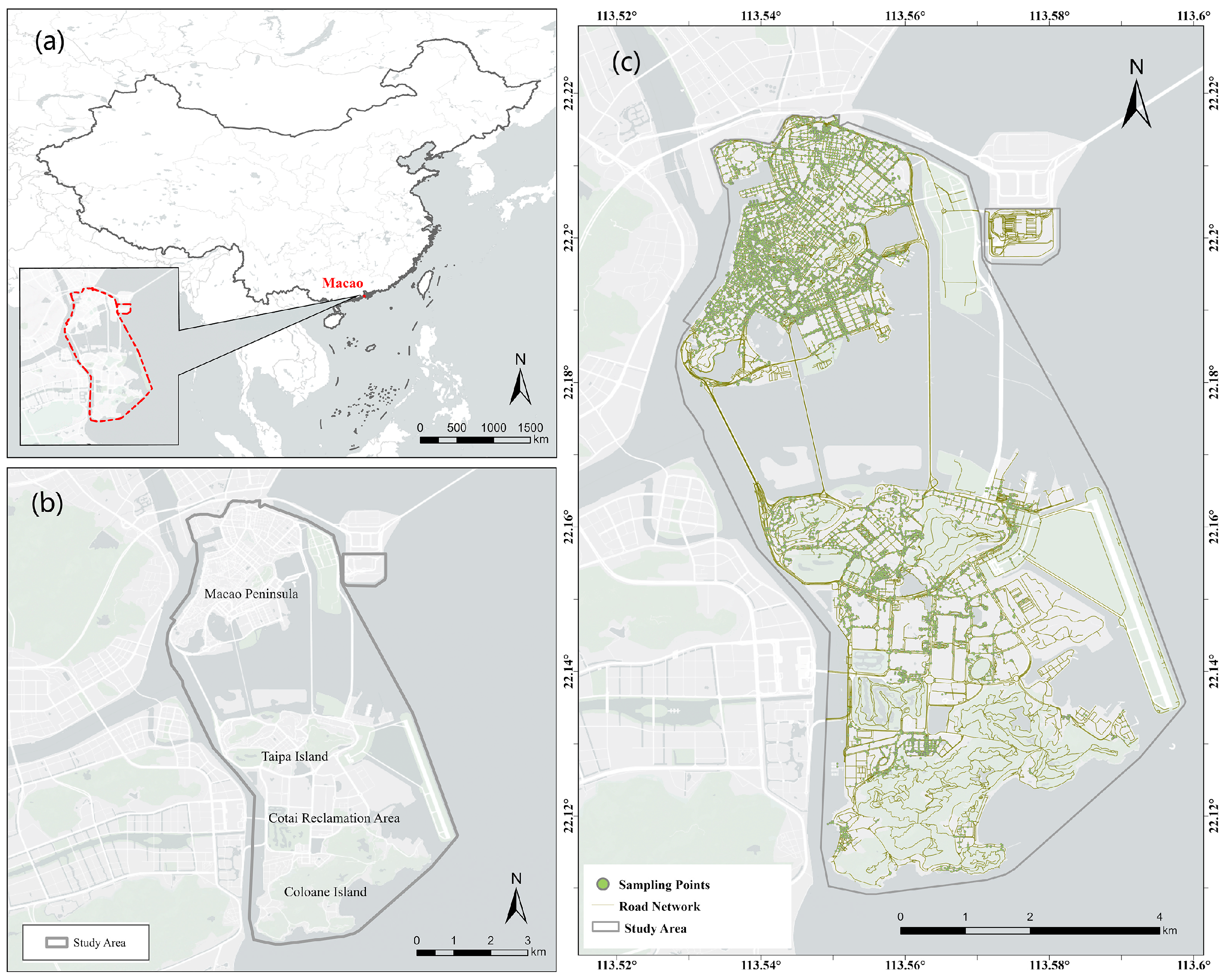
The Macao Special Administrative Region lies on the southern coast of China (22°07′–22°13′ N, 113°32′–113°36′ E) (Figure 1a), with a total area of about 33.3 km2, comprising the Macao Peninsula, Taipa Island, Coloane Island, and the Cotai reclamation area (Figure 1b). As one of the most densely populated cities in China, Macao accommodates more than 680,000 permanent residents within a built-up area of roughly 30 km2.
Macao’s urban spatial structure displays a pronounced historical stratification. The Macao Peninsula is the earliest developed core, with extremely high building density; its western and south-central parts preserve extensive Portuguese colonial architecture and traditional Chinese quarters, and the “Historic Centre of Macao” was inscribed on the UNESCO World Heritage List in 2005. The northern and eastern parts of the peninsula are dominated by high-rise residential and public housing developments built in the second half of the twentieth century. Taipa Island has a more heterogeneous urban fabric, where traditional villages, low- and mid-rise residences, and recently built commercial complexes coexist. The Cotai reclamation area, driven by the gaming and tourism industry over the past two decades, is a large-scale new development dominated by major hotels and commercial buildings. Coloane Island exhibits the lowest development intensity and retains more low-rise buildings and natural vegetation. This spatial structure provides the basic context for interpreting the geographical differentiation of building colors in the following sections.

2.1.2. Data Acquisition

Street-view imagery is used as the source of building façade color data. Based on OpenStreetMap (OSM) road network data, sampling points were uniformly placed along the city-wide road network at 50 m intervals. This interval approximates the typical façade width of buildings on urban streets and, within the pedestrian-scale visual range of about 100 m [34], ensures that each building is covered by at least one or two sampling points. At each sampling point, equirectangular panoramic images (resolution 4096 × 2048 pixels) were acquired through the Baidu Maps Open Platform API, fully recording the 360° × 180° scene around the point. Both the OSM road network and the street-view imagery were obtained in July 2025. For each point, the most recent panoramic image available at the time of acquisition was requested; because Baidu Street View is updated on a rolling basis and the API does not expose a reliable per-image capture date, the exact acquisition date of individual panoramas was not recorded. The implications of this temporal heterogeneity are discussed in Section 4.4.
A total of 10,671 original sampling points were generated. After removing points without street-view coverage or with inadequate image quality, 10,421 valid points remained (validity rate 97.7%). Based on semantic segmentation results, only building-class pixels were retained for subsequent color extraction. To ensure the reliability of façade color extraction, the Building Pixel Ratio (BPR) was defined as the ratio of building pixels to the total number of pixels in the image. Through stratified manual inspection, a threshold of BPR ≥ 5% was adopted to retain valid street-view images, yielding 8221 sampling points (Figure 1c). In the color-extraction stage, further area thresholding was applied to filter noise colors; the final analytical sample is reported in Section 3.1.

2.2. Image Processing Pipeline

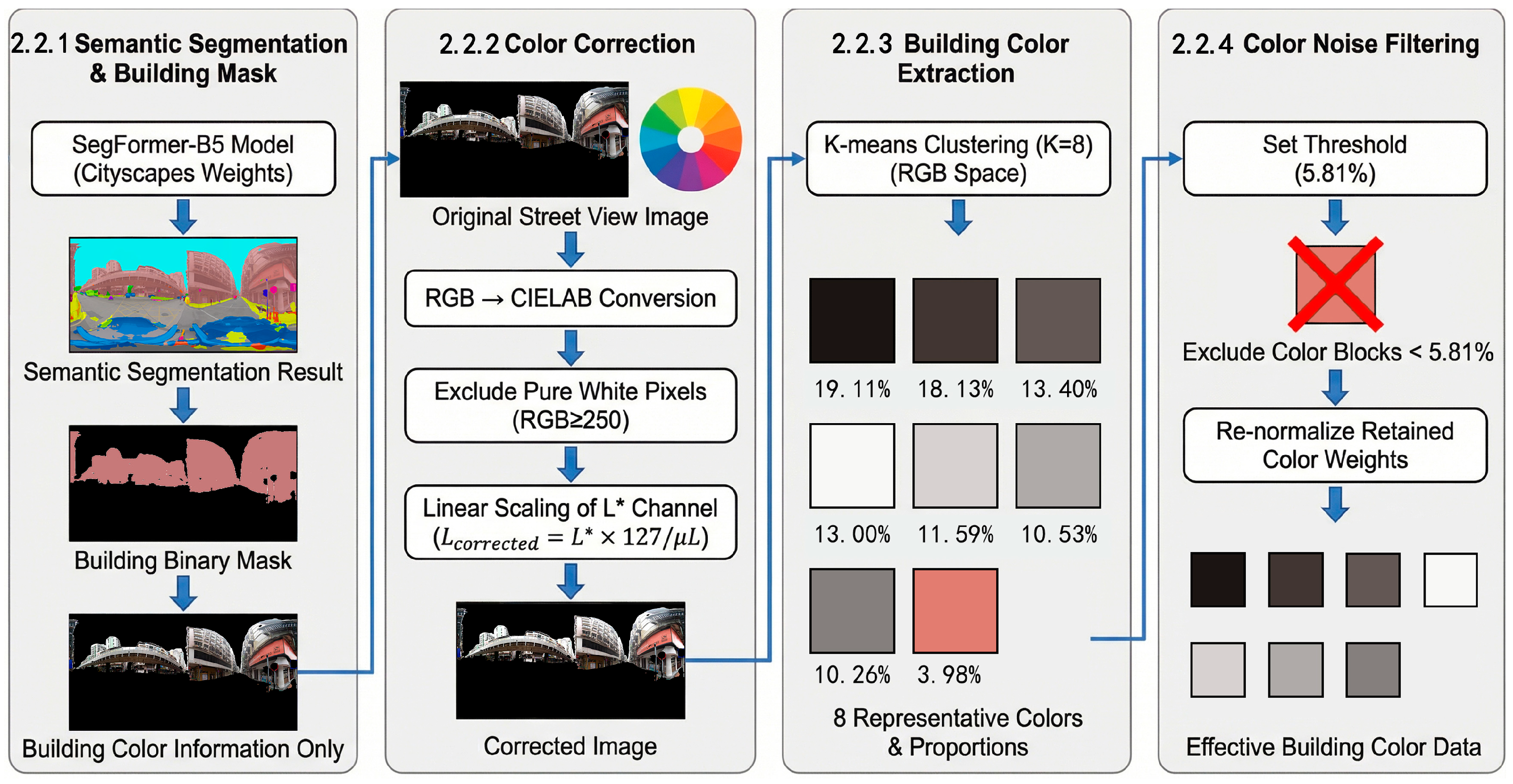
A complete processing pipeline was established to transform raw street-view imagery into quantitative building color data (Figure 2), comprising four stages: semantic segmentation and building masking, color correction, color extraction, and color-noise filtering.
All processing and analysis were implemented in Python (3.9.24): semantic segmentation used PyTorch (1.10.0) with MMSegmentation (0.11.0); color extraction and clustering, together with clustering-quality validation, used scikit-learn (1.6.1); statistical tests used SciPy (1.13.1); the global and local spatial autocorrelation statistics (Moran’s I) were implemented directly using SciPy and NumPy (2.0.2); and data handling and visualization used pandas (2.3.3), NumPy, and Matplotlib (3.9.4).

2.2.1. Semantic Segmentation and Building Masking

The SegFormer-B5 semantic segmentation model [35], implemented in the MMSegmentation framework, was used to perform pixel-level segmentation of each street-view image, with weights pre-trained on the Cityscapes dataset (mIoU = 82.4%). Sky regions, which the Cityscapes-trained model does not always delineate cleanly on panoramas, were additionally refined with Grounded-SAM [36] before mask generation. The segmentation output was converted into a binary building mask and overlaid on the color-corrected image to extract pixel-wise color information confined to building façades.

2.2.2. Color Correction

Street-view panoramas are affected by illumination conditions and automatic camera exposure, and as a result the same façade type can appear at noticeably different brightness levels across sampling points. To make façade luminance comparable across images, we apply a Gray-World-style [37] linear normalization to the L * channel only, with two design choices: (1) the reference mean is computed from building pixels (identified by the preceding semantic segmentation step, Section 2.2.1), not from the full panorama, because the analytical target is the comparability of building façade luminance specifically—using the full-panorama mean would dilute this signal with large sky, road, and vegetation regions whose brightness is unrelated to the façades being analyzed; and (2) only the L * channel is rescaled, while the chromaticity channels ( a * , b * ) are preserved unchanged, in order to remove brightness-level differences without altering the original façade chromatics (the chromatic implications of this partial correction are discussed in Section 4.4).
Pixels were converted from RGB to CIELAB 8-bit OpenCV LAB encoding ( L * scaled to 0–255); pure-white pixels (each RGB channel ≥ 250) were further excluded as residual sky regions that escaped semantic segmentation. For the remaining non-white building pixels, the L * channel was linearly scaled to a standard reference luminance:
L corrected *   =   L *   ×   127 μ L
where 127 is the midpoint of the L * channel and μ L is the mean L * of the non-white building pixels.
The effect of this correction was evaluated on the full set of 8163 analyzed panoramas. Before correction, the inter-image standard deviation of per-image μ L was 24.87 (in the 0–255 encoding); after correction it dropped to 3.09, a reduction of 87.6%, confirming that the procedure substantially homogenizes inter-image façade luminance. The mean μ L after correction is 124.95—slightly below the target value of 127—because the linear scaling is followed by clipping to the 0–255 range (an inherent constraint of 8-bit LAB encoding): heavily shaded panoramas with very low pre-correction μ L experience partial highlight clipping after rescaling, which leaves a small systematic offset between their post-correction mean and the target. In our dataset this clipping affects only an extreme minority of images—0.40% have μ L < 60 and 0.13% have μ L < 50—so the correction converges essentially to the target for the vast majority of panoramas. Representative before/after examples spanning the full illumination range are provided in Figure S1.

2.2.3. Color Extraction

For the building pixel regions of each image, the K-means clustering algorithm was applied in RGB space to extract K = 8 representative colors. The choice of K follows common practice in street-view-based urban color research: Wu & Zhang [38], Jiang et al. [30], and Song & Xiao [39] adopted similar cluster numbers in building color extraction from street-view imagery. Each extracted color is represented by the RGB value of its cluster centroid (also converted to HSV and CIELAB) and by its area share.

2.2.4. Color-Noise Filtering

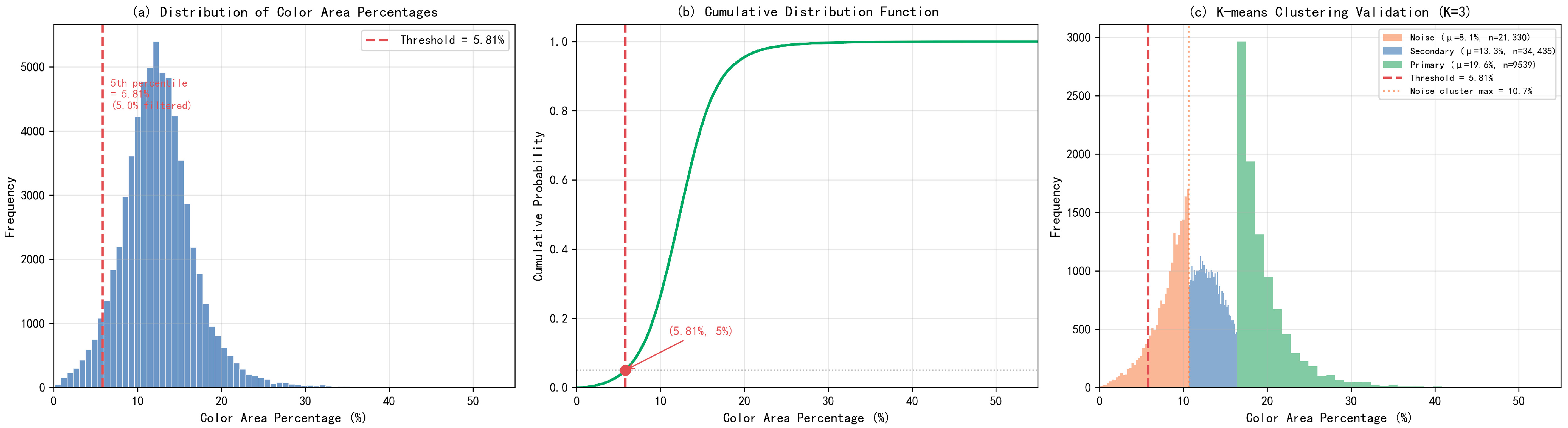
Some clusters returned by K-means occupy very small area shares and may represent visual noise such as stains, pipelines, or shadow edges. With reference to studies on perceptual thresholds of architectural color [40,41], and based on the fifth percentile of the area-share distribution of all 65,304 non-zero color patches in our dataset, a threshold of 5.81% was adopted for noise filtering (Figure 3). Colors with area shares below this threshold were removed, and the weights of the retained colors were re-normalized. After filtering, 98.8% of the sampling points retained six or more valid colors.

2.3. Construction of the Building Color Quality Evaluation Framework

2.3.1. Framework Overview

This study proposes the FCS (Fundamental–Compositional–Spatial) framework, which quantifies building color quality at three hierarchical layers (Table 2). The F layer (fundamental attributes, 4 indicators) describes the hue, saturation, value, and area share of the dominant color; the C layer (compositional structure, 4 indicators) evaluates the compositional quality among multiple colors; and the S layer (spatial association, 2 indicators) assesses the continuity and clustering of colors along the street spatial sequence.

2.3.2. F Layer: Fundamental Attributes of the Dominant Color

The dominant color C m a x is defined as the color with the largest area weight after noise filtering and weight re-normalization. The four indicators are specified as follows:
DH   =   H ( C max )
where DH is the dominant hue angle, a circular variable in [0°, 360°). Similarly:
DS   =   S ( C max ) / 100
DV = V ( C max ) / 100
DP = max ( w 1 ,   w 2 ,   ,   w N )
where w i is the normalized area weight of the i -th effective color.
It should be noted that DP in the F layer and HC in the C layer (defined in Section 2.3.3) are mathematically related: HC measures the standard deviation of color area weights, whereas DP is the maximum value of that weight series; when the dominant-color share increases, the deviation of the weight distribution from uniformity—that is, HC—necessarily increases as well. The two indicators, however, occupy non-overlapping roles within the FCS framework. DP is a fundamental descriptive indicator targeting the single dominant color: together with DH, DS, and DV, it constitutes a complete “hue–saturation–value–area” attribute portrait of the dominant color, addressing the descriptive question of how much area the dominant color occupies on a façade. HC is a compositional quality indicator targeting the multi-color weight distribution, characterizing the hierarchical orderliness of the entire chromatic series and addressing the evaluative question of how orderly the area allocation across colors is. DP and HC are therefore hierarchically complementary rather than conceptually redundant within the FCS framework: the former describes the “presence” of the dominant color, while the latter evaluates the “orderliness” of the color combination. The empirical manifestation of this mathematical coupling and its methodological implications for downstream multivariate modeling are presented in Section 3.3.

2.3.3. C Layer: Compositional Structure

All C-layer indicators are computed on the set of valid colors after noise filtering, with area weights incorporated.
  • Colorfulness (CF). Following Jiang et al. [30], whose measurement extends the algorithm of Hasler and Süsstrunk [20] with area weighting, the RGB value of each color is transformed into opponent components:
r g i = | R i G i | ,     y b i = | 0.5 ( R i + G i ) B i |
The area-weighted means ( μ rg , μ yb ) and area-weighted dispersions ( σ rg , σ yb ) are then computed, giving:
CF =   σ rg 2   +   σ yb 2   +   0.3   × μ rg 2   +   μ yb 2
Here μ rg and μ yb denote the area-weighted means of the opponent-color components, capturing overall chromatic intensity, while σ rg and σ yb denote the corresponding area-weighted dispersions, capturing chromatic variety. Computing both with area weights ensures that color patches occupying larger façade areas contribute proportionally to CF. The weight 0.3 balancing variety and intensity follows the original Hasler and Süsstrunk formulation [20].
  • Color Harmony (CH). Based on the two-color harmony model of Ou and Luo [22], three components are combined in CIELAB space: the chromatic effect H C , the lightness effect H L , and the hue effect H H . For any pair of colors ( c i , c j ) :
C H ij = H C + H L +   H H
with:
H C   =   0.04   +   0.53 tan h ( 0.8 0.045 Δ C ) ,   Δ C   =   Δ H ab * 2   +   ( Δ C ab * / 1.46 ) 2
In this expression, Δ C combines the CIELAB hue difference Δ H ab * and the chroma difference Δ C ab * , with the chroma difference scaled by the factor 1.46 to balance the contribution of hue and chroma to perceived harmony, as established in the original Ou and Luo model [22]; the hyperbolic-tangent form maps these color differences onto a bounded chromatic-harmony contribution.
H L is composed of a lightness-sum effect and a lightness-difference effect; H H is obtained by computing the hue-harmony contribution HSY of each color independently and then summing and includes a chroma correction factor, a hue-dependent function, and a yellow effect term. The pairwise harmony values over all valid color pairs are aggregated as a weighted average using the product of area weights:
CH =   i < j w ij · C H ij i < j w ij , w ij   =   w i · w j
Because this model was originally derived from psychophysical experiments on uniform color pairs, extending it to the multi-color setting of real façades—by computing pairwise harmony over all valid colors—follows an established line of street-view-based building-color research that applies color-harmony evaluation to segmented façade colors at scale [21]. We adopt the area-weighted pairwise aggregation so that colors occupying larger façade areas contribute proportionally to the overall harmony score, consistent with the compositional emphasis of the C layer. The perceptual validity of this extension is considered further in Section 4.4.
  • Color Contrast (CC). Using the CIELAB Euclidean color difference ( Δ E ab * ; [42]) between all valid color pairs, we compute the weighted sum:
CC = i = 1 N j = i + 1 N ( w i · w j ) · Δ E ij
  • Hierarchy Clarity (HC). This indicator measures the orderliness of the area distribution among colors:
HC = 1 N i = 1 N ( w i w ¯ ) 2
where w ¯ =   1 / N is the theoretical mean under a uniform distribution. A higher HC indicates a more differentiated chromatic hierarchy.

2.3.4. S-Layer: Spatial Association

  • Street Color Similarity (SCS). Extending the inter-image color-similarity measure of Jiang et al. [30], we use a kernel cosine similarity in CIELAB space to directly compare the weighted color distributions of two sampling points. For any two points i and j , the weighted kernel inner product is computed as:
K ij = k = 1 N i l = 1 N j w ik · w jl · exp Δ E ( c ik ,   c jl ) 2 2 τ 2
After normalization, the kernel cosine similarity is obtained as:
Sim ( i ,   j )   =   K ij K ii · K jj
The Gaussian kernel assigns higher similarity to color pairs with smaller perceptual difference Δ E , so that the kernel cosine similarity Sim ( i ,   j ) increases when neighboring sampling points share perceptually close colors; the bandwidth τ controls how quickly the contribution of a color pair decays as their perceptual difference grows.
The SCS value of each sampling point is the mean similarity with all spatial neighbors within a search radius of 100 m. The kernel bandwidth τ =   20 corresponds to the CIELAB perceptual threshold of “markedly different but within the same color family [26]”.
  • Color Spatial Autocorrelation (CSA). Color contrast (CC) is selected as the target variable, and the Local Moran’s I of Anselin [33] is computed:
I i = ( x i x ¯ ) σ 2 j = 1 N w ij ( x j x ¯ )
The spatial weights matrix is defined on a fixed distance band of 100 m and row-standardized. Statistical significance at each point is evaluated through a permutation test (n = 999, α = 0.05), and significant points are classified into HH, LL, HL, and LH; non-significant points are labeled NS. The Global Moran’s I is also reported as an overall measure of city-wide spatial autocorrelation.

2.4. Identification of Color Quality Types

The K-means clustering algorithm is applied using the six C+S-layer indicators (CF, CH, CC, HC, SCS, CSA) as input variables. The C+S layers are used rather than all ten indicators because: (a) F-layer indicators are descriptive attributes and do not directly reflect color quality; (b) DH in the F layer is a circular variable that cannot be correctly handled by Euclidean distance; (c) keeping F-layer indicators as external variables allows post hoc analysis of the color-attribute differences across quality types; and (d) the mathematical coupling between F-layer DP and C-layer HC (see Section 2.3.2) makes it inappropriate to include both as inputs in multivariate analysis, further supporting the choice to use only C+S-layer indicators as clustering inputs. Crucially, excluding the F layer from clustering does not preclude its use afterwards: because the F-layer indicators are not part of the clustering input, they serve as independent external variables against which the resulting types can be characterized and validated post hoc (Section 3.6.2). The fundamental color attributes used later to label and describe the types (e.g., their lightness or saturation profiles) are therefore derived from this independent post hoc comparison, not from the clustering itself. Z-score standardization is applied before clustering. The algorithm uses K-means++ initialization, ninit = 50, and a maximum of 300 iterations.
The optimal cluster number is determined jointly by the elbow method, the silhouette coefficient, and the Calinski–Harabasz index over K = 2–10. Clustering quality is validated along three dimensions: internal validation (silhouette coefficient, Calinski–Harabasz index, Davies–Bouldin index), consistency validation (ARI between K-means and Ward hierarchical clustering), and stability validation (mean ARI over 50 rounds of 80% subsampling).

2.5. Spatial Mapping and Statistical Testing of Quality Types

FCS indicator values and cluster labels are mapped to the geographic coordinates of sampling points to generate spatial distribution maps. Differences among the four types in F-layer indicators are tested using the Kruskal–Wallis non-parametric test for the linear variables (DS, DV, DP). For dominant hue (DH), which is a circular variable for which the Kruskal–Wallis test is not valid, between-type differences are assessed by a sine/cosine decomposition (each component tested by Kruskal–Wallis), complemented by the Watson–Williams test (circular ANOVA) as a parametric corroboration.

3. Results

3.1. Data Overview and Indicator Statistics

After the complete processing pipeline—street-view acquisition, BPR screening (BPR ≥ 5%), semantic segmentation, color correction, K-means color extraction, and area-threshold noise filtering (5.81%)—8163 sampling points were finally retained for analysis. All eight F-layer and C-layer indicators were successfully computed for every sample. For the S layer, 51 sampling points were excluded from SCS and CSA computation because no spatial neighbor existed within the 100 m search radius, leaving 8112 points for the S-layer analyses and subsequent clustering. These 51 isolated points are located exclusively along the edges of the study area, corresponding to coastal headlands, cross-channel road segments, and the outer perimeters of reclaimed areas. Figure S2 maps them over the full sampling grid, showing that each is visibly separated from its surroundings and that none falls within the city’s densely sampled built-up cores; the exclusion therefore reflects the geometry of the study area rather than data gaps in its analytically important built-up zones.
Table 3 summarizes the descriptive statistics of the ten FCS indicators. Among F-layer indicators, the mean of dominant hue (DH) is 76.5°—far higher than its median of 39.0°—showing a strongly right-skewed distribution: a small number of cool-toned samples inflate the mean, while the majority of buildings are concentrated in the warm-hue range. Dominant value (DV) has the largest standard deviation among F-layer indicators (0.265) and spans almost the full range (0.051–0.996), hinting at a bimodal structure along the value dimension. Within the C layer, color contrast (CC) has the closest-to-normal distribution (mean 14.98, median 15.25), whereas colorfulness (CF) and color harmony (CH) are both skewed. In the S layer, the mean street color similarity (SCS) is as high as 0.946, indicating that street color is overall spatially continuous; color spatial autocorrelation (CSA) is strongly right-skewed (median 0.195, maximum 19.67), with a small number of sampling points exhibiting extremely strong spatial clustering. The spatial patterns and associations of the indicators will be examined in the sections that follow.

3.2. Overall Chromatic Profile of Macao’s Buildings

3.2.1. Hue Composition and Chromatic Tendencies

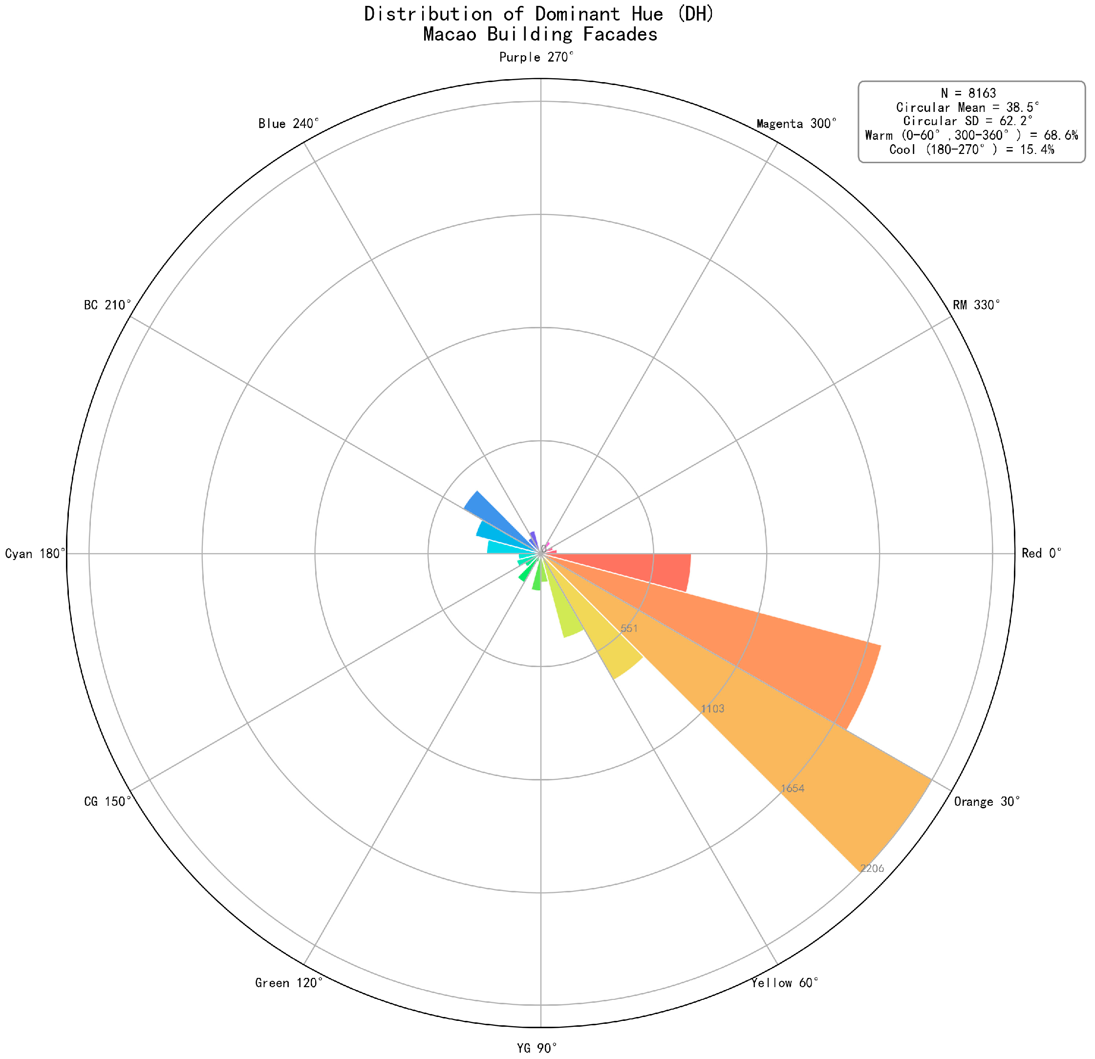
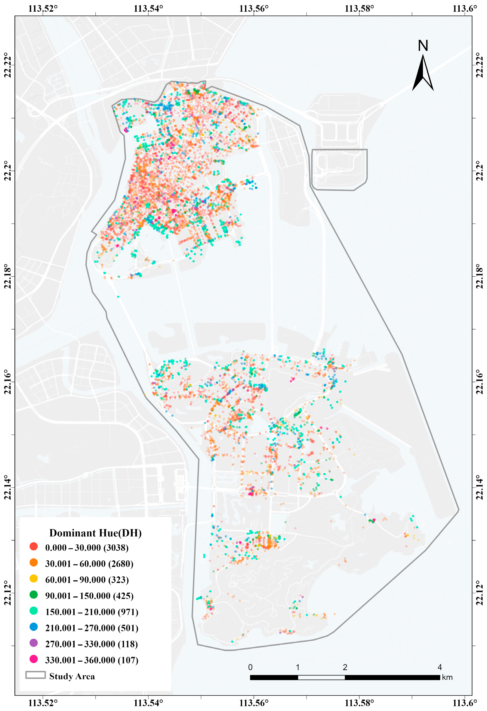
Figure 4 presents the circular distribution of dominant hue (DH). Macao’s building colors show a highly concentrated warm profile: the circular mean is 38.5° (orange range) and the circular standard deviation is 62.2°. The warm sector (0–60° and 300–360°) accounts for 68.6% of all samples, while the cool sector (180–270°) accounts for only 15.4%, giving a warm-to-cool ratio of approximately 4.5:1. In particular, the 0–60° range (red-orange to orange-yellow) contains 5718 sampling points (70.0%), forming a remarkably pronounced unimodal concentration (Figure 5). This distribution aligns closely with the intrinsic color of Macao’s traditional masonry and stucco materials and the historical preference for warm-toned coatings on Portuguese-style buildings. Within the cool sector, the 150–210° range (cyan hues) forms a secondary peak with 971 sampling points (11.9%), possibly attributable to façade paints in cyan-gray tones adopted by some buildings.
Spatially (Figure 5), the Macao Peninsula is dominated by red and orange points, with warm samples particularly dense in its central-western part. The hue composition on Taipa Island is more diverse, with markedly higher frequencies of cyan, blue, and green samples than on the peninsula, forming a more pronounced alternation of warm and cool tones. This differentiation suggests that the spatial structure of hue is linked to the historical phasing of urban construction, which is further examined through the cluster analysis in Section 3.5.

3.2.2. Saturation and Value Patterns

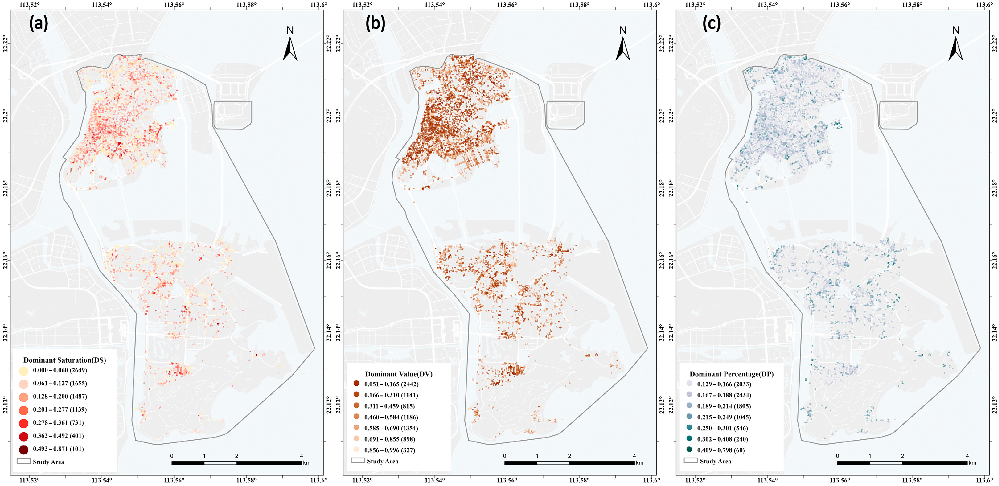
Figure 6 presents the spatial distribution of dominant saturation (DS), dominant value (DV), and dominant percentage (DP), revealing three noteworthy features.
First, Macao’s building colors are overall low in saturation. The median DS is only 0.116, and more than half of the sampling points (52.7%) have DS below 0.127, visually approaching gray. Spatially, medium-to-high saturation samples are concentrated in the central-southern part of the Macao Peninsula—a region that largely overlaps with the core of the historic district, where the warm-yellow and ochre-red stucco coatings typical of Portuguese-style buildings are a main source of relatively high saturation. The northern peninsula and the outer islands are dominated by low saturation, consistent with modern buildings that extensively employ gray concrete or light-colored coatings (Figure 6a).
Second, value exhibits a bimodal distribution. DV shows the largest variability among F-layer indicators (SD = 0.265); the banded statistics reveal a bimodal structure: the lowest band (DV ≤ 0.165) contains 2442 sampling points (29.9%), the medium-to-high band (DV = 0.585–0.690) contains 1354 (16.6%), while the intermediate range between the two bands contains only 815 points (10.0%). Spatially, the central-western peninsula is covered by large areas of dark-value points, coinciding with the high-density old urban clusters; the eastern coastal strip of the peninsula and the newly built areas on the outer islands are dominated by medium-to-high values, forming a “dark-west, bright-east” gradient (Figure 6b). The spatial co-variation between DS and DV reveals two chromatic modes: the “dark-yet-colored” mode of the historic built-up zones (low value, moderate saturation) versus the “bright-yet-colorless” mode of modern construction areas (high value, low saturation). This differentiation is, to a large extent, the chromatic projection of the city’s historical construction strata.
Third, in contrast to the pronounced spatial differentiation of DS and DV, DP is distributed remarkably evenly across the city (SD = 0.048): at 76.8% of sampling points, the dominant-color share falls within a narrow range of 13–21%. This “differentiated attributes but uniform structure” phenomenon suggests that the areal hierarchy of façade colors is driven more by physical form (the area ratios of doors, windows, balconies, and attached components) than by chromatic design intent (Figure 6c).

3.3. Compositional Quality of Building Colors

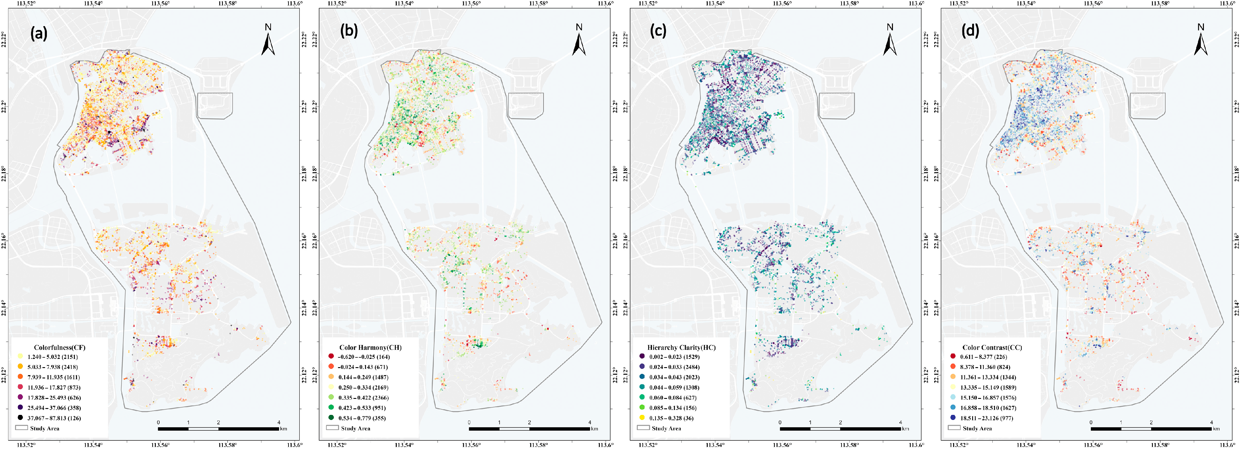
Figure 7 displays the spatial distributions of the four C-layer indicators. Both colorfulness (CF) and color contrast (CC) show a spatial gradient with high values concentrated on the Macao Peninsula and low values in the outer islands: the central-western peninsula contains dense clusters of high-CF (>25) and high-CC (>16) patches, while Taipa, Cotai, and Coloane are dominated by low values. The spatial distribution of color harmony (CH) is comparatively uniform, with the overwhelming majority of samples taking positive values; the peninsula as a whole shows a medium-to-high harmony level, with only sporadic negative-valued points. Hierarchy clarity (HC) is generally low (mean = 0.037), but the outer islands—especially central-southern Taipa—contain many points with high HC (>0.06), suggesting that more façades in that area are dominated by a single color. Notably, CC and CH show a degree of spatial co-variation: regions with high harmony tend also to exhibit higher contrast, indicating that moderate chromatic differences contribute to, rather than undermine, the perception of harmony.
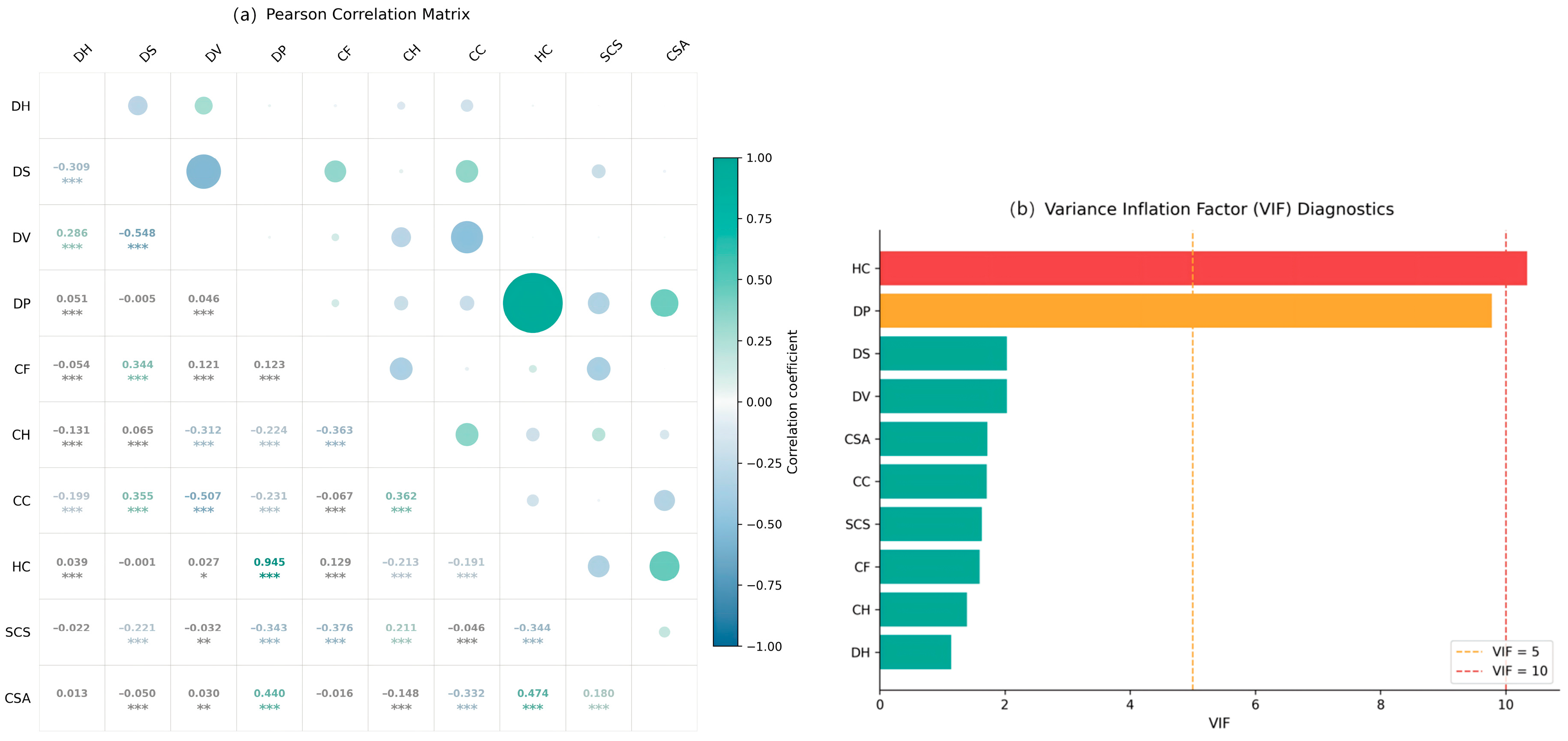
To comprehensively examine the statistical structure within the FCS system, both Pearson correlation matrices and variance inflation factor (VIF) diagnostics were computed for all ten indicators (Figure 8a,b). The diagnostics reveal one expected strong association: DP and HC exhibit high collinearity (Pearson r = 0.945; VIF for DP = 9.78, VIF for HC = 10.34). This association arises from the mathematical coupling between the two indicators by definition (see Section 2.3.2) and reflects the cross-layer structural connection of the FCS system rather than design redundancy—F-layer DP serves the descriptive characterization of the dominant color, whereas C-layer HC serves the evaluative assessment of multi-color compositional orderliness. Excluding the DP–HC pair, the remaining eight indicators all show VIF below 2.1 in the full 10-indicator diagnostic (max VIF = 2.03 for DS), indicating that the high collinearity is structurally confined to this single cross-layer pair while the rest of the FCS system possesses sufficient indicator independence. The strongest pairwise correlations among these remaining eight indicators occur between DS and DV (r = −0.548) and between DV and CC (r = −0.507), both of which are conceptually expected: lighter (higher DV) building façades tend to use lower-saturation paint, and darker façades tend to involve stronger inter-color contrasts in CIELAB space.
Within the six C+S-layer indicators that are jointly used as clustering inputs (Figure 8a), several substantively meaningful associations emerge. Two main associations are observed within the C layer: CF and CH show a moderate negative correlation (r = −0.363), revealing the intrinsic tension between colorfulness and harmony, while CH and CC show a moderate positive correlation (r = 0.362), indicating that moderate CIELAB color differences are a constituent element of harmonious combinations rather than their opposite. CF and CC are nearly uncorrelated (r = −0.067), confirming that the two capture different dimensions. Between the C and S layers, the most prominent association is the positive correlation between HC and CSA (r = 0.474)—the strongest coefficient among the six clustering inputs—indicating that single-color-dominated façades tend to cluster in space. CF and SCS are negatively correlated (r = −0.376), suggesting that vividly colored buildings reduce street visual continuity. It should be noted, however, that this association is partly intrinsic to how the two indicators are constructed: façades with high CF inherently carry more distinctive color profiles and therefore tend to show lower kernel cosine similarity with their neighbors, independently of any substantive contrast in urban color composition. The negative CF–SCS correlation should therefore be read as a combination of this methodological coupling and a substantive street-continuity effect, rather than as a pure measure of the latter. CC and CSA are negatively correlated (r = −0.332), meaning that high-contrast buildings tend to occur in areas of high chromatic heterogeneity. The maximum |r| among the six C+S-layer clustering inputs is 0.474, below the 0.5 redundancy threshold, indicating that they capture different dimensions of color quality and are jointly suitable as clustering inputs.

3.4. Spatial Continuity and Clustering of Street Colors

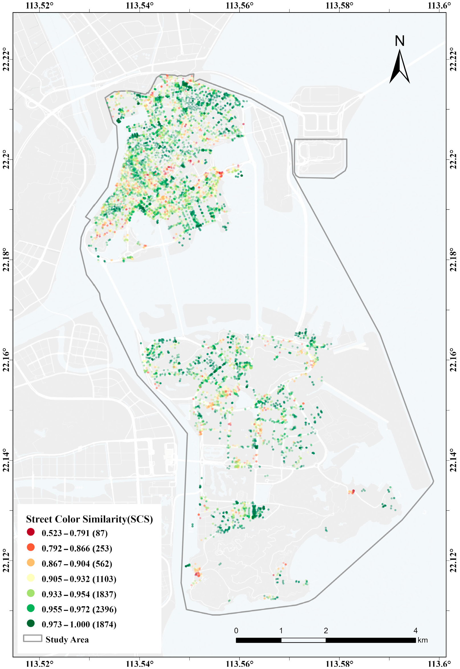
The mean street color similarity (SCS) is 0.946 (SD = 0.040), indicating that Macao’s street colors are overall highly continuous in space (Figure 9). High-SCS areas (>0.955) are widely distributed across the north-eastern Macao Peninsula and most of the outer islands, corresponding to residential precincts of similar vintage and unified materials. Low-SCS points (<0.90) are limited in number (n = 902, 11.1%) and are scattered mainly in the central-western and southern peninsula and at the southern tip of Coloane Island, marking locations where abrupt chromatic changes occur between neighboring buildings. Although such color-break points are few in number, they are diagnostically valuable for urban color management and can be used to locate hotspots of chromatic conflict.
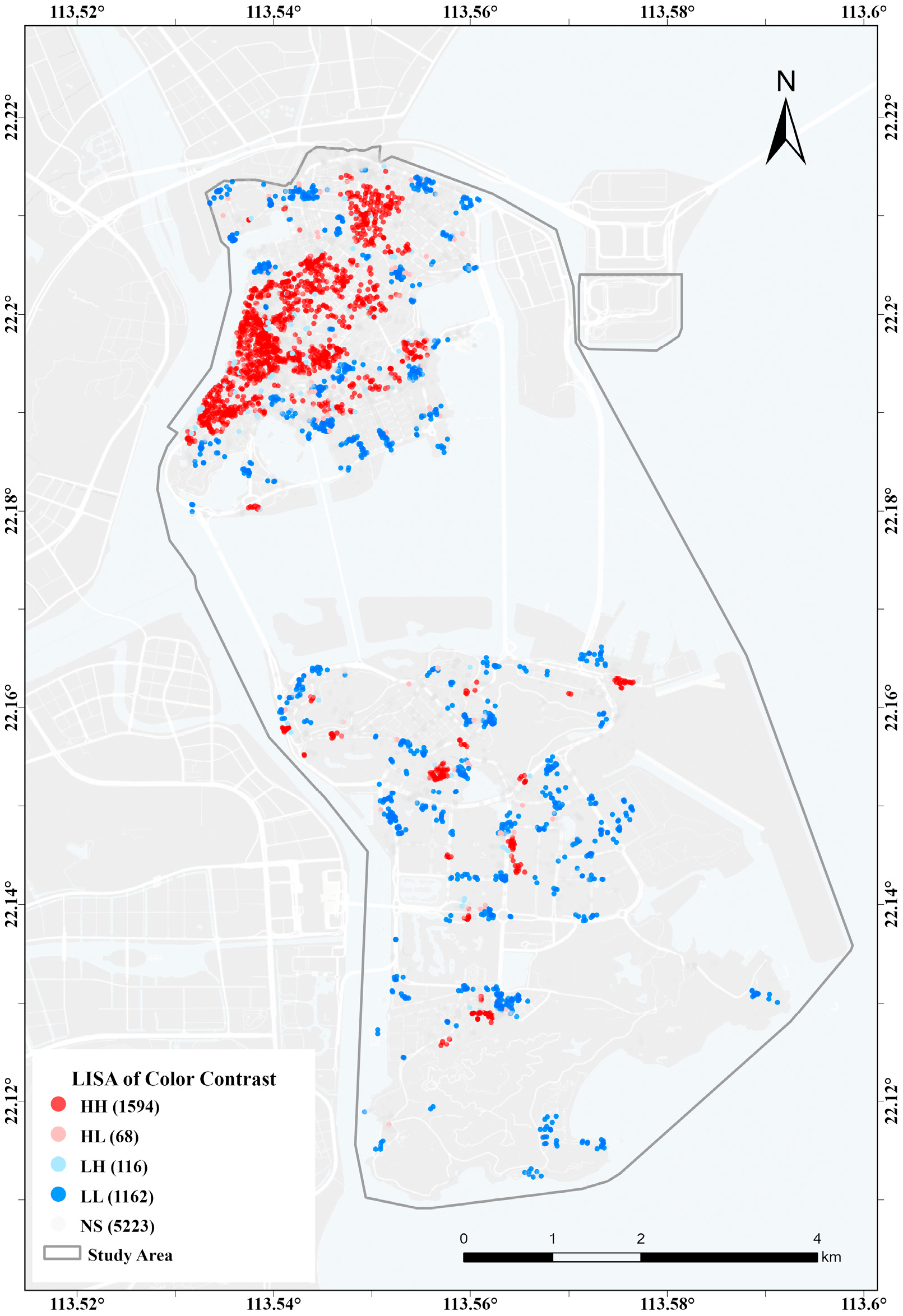
The global spatial autocorrelation of color contrast (CC) yields Global Moran’s I = 0.456 (z = 108.35, p = 0.001), indicating highly significant positive spatial autocorrelation: high-contrast buildings tend to adjoin high-contrast buildings, and low-contrast buildings likewise cluster together. The LISA analysis at p < 0.05 identifies 2940 significant points (36.1%), whose spatial pattern presents a clear “block structure” (Figure 10). The HH cluster (n = 1594) forms large continuous patches in the central-southern peninsula and constitutes the most pronounced high-contrast agglomeration in the city; this area largely coincides with the “dark-yet-colored” historical building zone identified in Section 3.2. The LL cluster (n = 1162) is distributed mainly in the northern peripheral strip of the peninsula and at several locations in the outer islands, corresponding to areas of soft and homogeneous color, presumably associated with unified residential developments. Spatial outliers (HL = 68, LH = 116) are sparse and scattered, and do not form significant spatial patterns. The complementary spatial distribution of HH and LL regions indicates that Macao’s color-contrast pattern is structurally driven by construction timing and planning zoning rather than being random.

3.5. Color Quality Types

3.5.1. Determining and Validating the Optimal Cluster Number

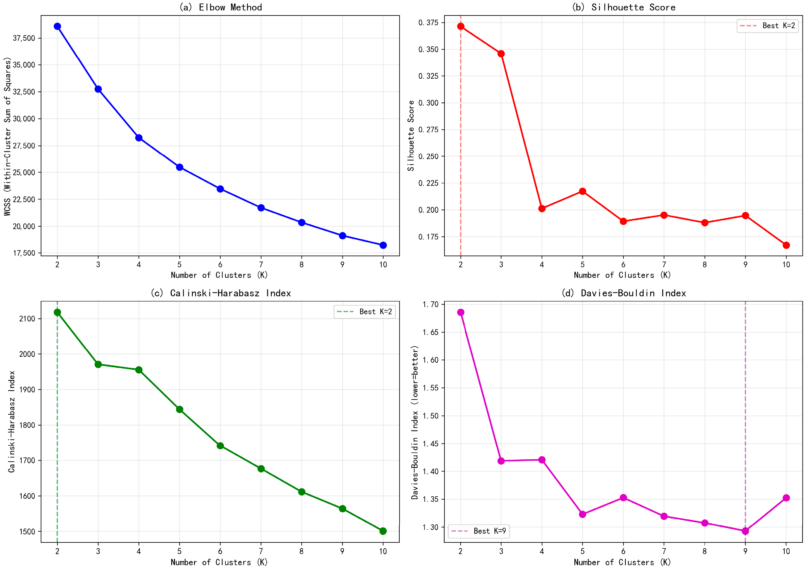
Using the six C+S-layer indicators as input, K-means clustering was performed on the 8112 valid sampling points. Figure 11 presents clustering-quality evaluation results for K = 2–10. Both the silhouette coefficient and the Calinski–Harabasz index peak at K = 2, but this partition is too coarse to support differentiated color governance. The WCSS curve shows an apparent slope change between K = 3 and K = 4, and the Davies–Bouldin index stabilizes from K ≥ 3 (between 1.29 and 1.42). Considering both statistical indicators and planning utility, K = 4 was selected.
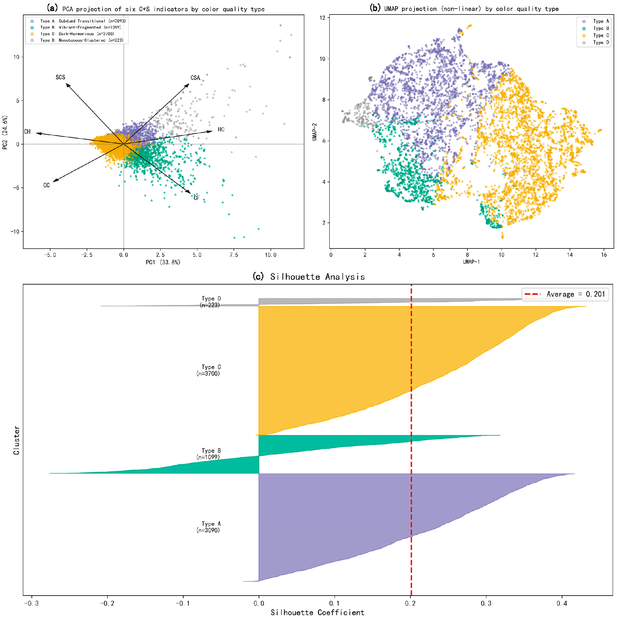
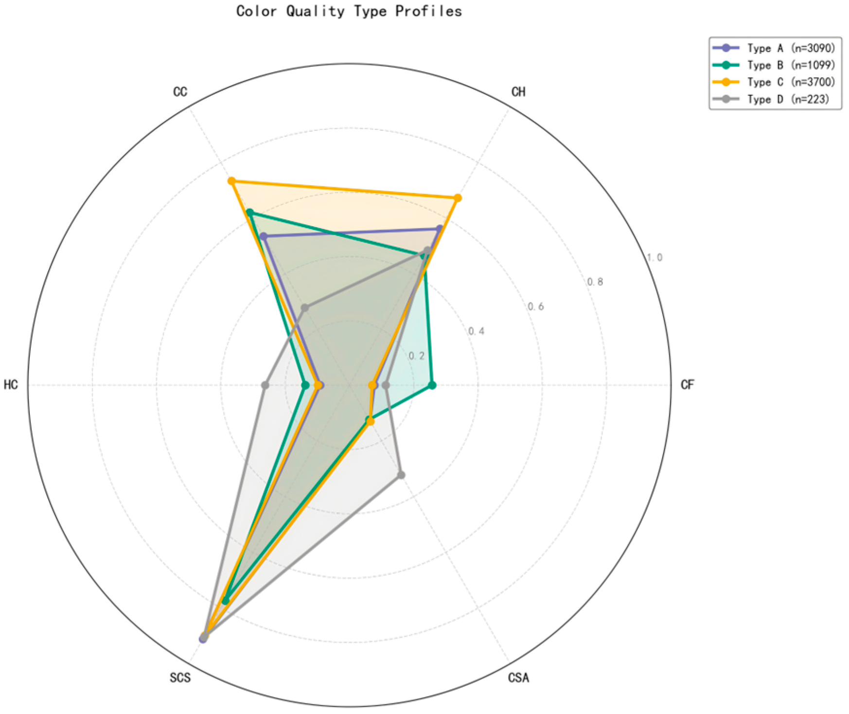
Clustering-quality validation results are summarized in Table 4. At K = 4, the silhouette coefficient is 0.201. Rather than indicating an unreliable partition, this moderate value reflects the continuously graded nature of urban color data, in which a large proportion of sampling points occupy transitional positions between types. Three lines of evidence support this interpretation. First, the PCA projection of the six standardized clustering inputs (Figure 12a) shows that each type occupies a distinct core region oriented along interpretable indicator-loading directions, yet adjacent types grade continuously into one another rather than forming disjoint islands—precisely the geometry that lowers the silhouette coefficient while preserving meaningful structure; the non-linear UMAP projection (Figure 12b) confirms the same pattern. Second, a fuzzy c-means analysis on the same inputs shows that 93.1% of points have a maximum membership below 0.6 (Table 4), confirming that most façades genuinely lie between prototypes rather than belonging unambiguously to a single cluster. Third, despite the moderate silhouette, the partition is highly reproducible, with a mean ARI of 0.968 ± 0.026 over 50 rounds of 80% subsampling (Table 4). We therefore retain K-means for its interpretability and reproducibility, while explicitly noting its inherent limitation: as a hard-partition method it assigns each point to a single type and thus imposes crisp boundaries on a fundamentally continuous chromatic gradient, so the four types should be read as characteristic prototypes rather than sharply bounded, mutually exclusive categories.
The ARI between K-means and Ward hierarchical clustering is 0.265, indicating that the two algorithms, optimizing different objectives, produce distinct partitions. The silhouette analysis (Figure 12c) shows that Types C and A are the largest in size and contain almost exclusively positive silhouette values; Type B is concentrated in the positive range; and Type D, although the smallest, has distinctive indicator profiles that justify its recognition as an independent type.

3.5.2. Indicator Profiles of the Four Color Quality Types

Table 5 and Figure 13 present the indicator profiles of the four types. The four types are labeled by combining their C+S-layer profiles (described below and shown in the radar charts) with their fundamental color attributes, the latter established through the independent post hoc tests reported in Section 3.6.2. Each label thus summarizes both how the colors are composed and arranged (C+S layers) and the dominant-color attributes that statistically distinguish the type (F layer); the descriptor “dark,” for instance, reflects the significantly lower dominant value of that type confirmed in Section 3.6.2, rather than any clustering input.
Type A—Subdued-Transitional (38.1%). All indicators sit at medium levels, with relatively low CF (7.97) and CC (12.92) and high SCS (0.958). The radar profile is well-balanced with no pronounced peaks or troughs, representing modern built-up areas without a distinctive chromatic character.
Type B—Vibrant-Fragmented (13.5%). CF is far higher than in the other types (23.47), while CH is the lowest (0.156) and SCS is the lowest (0.892). The radar profile shows a marked outward extension along the CF axis and an inward contraction along CH and SCS, forming a distinctive “vivid but disharmonious, visually fragmented” contour.
Type C—Dark-Harmonious (45.6%). The largest type, with the highest CH (0.397) and the highest CC (17.27) co-occurring, and the lowest CF (7.36). The radar profile extends simultaneously along the CH and CC axes, forming a characteristic upper-left extension, i.e., a “high-contrast yet highly harmonious” profile that represents the historical chromatic substrate of Macao.
Type D—Monotonous-Clustered (2.7%). The smallest type but with a very distinctive profile: CC is extremely low (7.27, 49% of the city-wide mean), HC is the highest (0.088, more than twice the other types), and CSA is extremely high (4.63, more than ten times the other types). The radar profile extends sharply along the CSA axis and prominently along the HC axis while contracting deeply along the CC axis, indicating “homogeneous color islands” that are absolutely dominated by a single color and highly clustered in space.

3.6. Spatial Pattern of Quality Types and Differences in Fundamental Attributes

3.6.1. Spatial Distribution of the Four Color Quality Types

Figure 14 shows the spatial distribution of the four types. Type C (Dark-Harmonious, 45.6%) is the most widely distributed, forming large continuous patches in the central-western and southern Macao Peninsula—the main chromatic substrate of the city—and also concentrating in central Taipa. Type A (Subdued-Transitional, 38.1%) is spatially complementary to Type C, mainly located in the northern and north-eastern peninsula and appearing as strips or scattered points along main roads in the outer islands, together forming a mosaic pattern. Type B (Vibrant-Fragmented, 13.5%) does not form large continuous patches; instead, it appears as scattered nodes embedded in the surrounding subdued or harmonious fabric, with several small aggregations in the central and south-western peninsula. Type D (Monotonous-Clustered, 2.7%) is the smallest type yet forms several cluster-shaped aggregations in the central-southern outer islands and the northern tip of the peninsula, consistent with its extremely high CSA values—monotonous-color buildings occur in the form of “homogeneous color islands” and presumably correspond to large residential complexes developed under unified planning.
The overall spatial pattern reflects a geographical logic tied to the city’s development trajectory: Type C dominates the historic core, Type A fills the newer residential zones, Type B is scattered across commercial and tourism-active nodes, and Type D marks specific parcels developed uniformly at large scale.

3.6.2. Differences in Fundamental Color Attributes Across Types

Tests on the four F-layer indicators reveal highly significant differences across the four types for every indicator (p < 0.001; Kruskal–Wallis for DS, DV, and DP, and the circular test described in Section 2.5 for DH). This demonstrates that the partition driven by the C+S layers also corresponds to systematically and significantly different fundamental color attributes—the statistical basis on which the four types are named and characterized in terms of their dominant-color properties (Table 6, Figure 15).
Value (DV) is the most discriminating indicator (H = 2327.0). The mean DV of Type C is only 0.261, with the box entirely at the lowest level, clearly confirming its “dark” designation; Type D (0.566) and Type A (0.540) are medium-to-high in value, while Type B sits between them (0.478). Saturation (DS) is the next most discriminating (H = 1285.3): Type B has the highest mean DS (0.205), more than twice that of Type A (0.091) and Type D (0.084), corroborating its “vibrant” designation, while Type C ranks second (0.179), with moderate saturation underpinning its harmonic profile. For dominant percentage (DP; H = 902.9), Type D reaches 0.320—far above the other types. This is consistent with the extreme HC value of Type D (0.088) reported in Section 3.5.2 and reflects the mathematical coupling between DP and HC (see Section 2.3.2): the two indicators jointly characterize the extreme chromatic homogenization of Type D façades from two complementary perspectives—the “presence” of the dominant color (DP = 0.320, occupying nearly one-third of the façade area) and the “orderliness” of the overall weight series (HC = 0.088, indicating high deviation from uniform area distribution)—jointly confirming the “monotonous” designation. For hue (DH), because hue is a circular variable for which the Kruskal–Wallis test is not appropriate, between-type differences were assessed by decomposing DH into sine and cosine components and testing each by Kruskal–Wallis, both of which were highly significant (p < 0.001); the Watson–Williams test (circular ANOVA) gave consistent results (F(3, 8108) = 28.74, p < 0.001; see Table 6 note). Type C has the lowest circular median (34.3°) and the most concentrated distribution (mean resultant length R = 0.715), with hues tightly clustered in the orange range; Type A is the most dispersed (R = 0.378), spanning from warm to cool hues, while Types B and D fall in between.
Taken together, the four types show clear chromatic portraits: Type A represents “light, low-saturated, hue-dispersed” neutral buildings; Type B represents “medium-value, highly saturated” vivid buildings; Type C represents “dark, moderately saturated, warm-hue-consistent” historic buildings; and Type D represents “light, low-saturated, single-color-dominated” uniformly planned buildings.

3.6.3. Typical Street-View Examples

Table 7 lists the sampling points closest to the cluster centers of each type. Type A (Image 8844) has CF = 6.79 and CC = 12.22 with no extreme values along any dimension, typifying chromatic “moderation.” Type B (Image 9241) has CF as high as 25.22, while CH drops to 0.179 and SCS to 0.898; its vivid palette is not only poorly harmonized internally but also produces a strong chromatic break with neighboring buildings. Type C (Image 8536) has CH (0.397) and CC (16.85) simultaneously at high levels, yielding a “rich but not chaotic” visual effect. Type D (Image 12160) has CC of only 6.46, HC up to 0.093, and CSA of 4.93, pointing to a façade absolutely dominated by a single color at the core of a “chromatically homogeneous zone”. Representative street-view images of the four types are shown in Figure 16.

4. Discussion

4.1. The Necessity of Multi-Dimensional Evaluation: Findings That Go Beyond Dominant Color

Urban building color research has long taken dominant-color description as its core paradigm, characterizing urban color through the basic attributes of the dominant color after color information is extracted. This paradigm rests on an implicit premise: that the dominant color is sufficient to represent the chromatic content of a façade. Existing Macao color studies largely inherit this tradition—whether the street-façade analysis based on color-card matching [5], the Pantone-based chromatic archive of the historic center [43], or hue–lightness comparisons between Chinese- and Western-style buildings [44]—and all take dominant-color attributes as their object of analysis. The F-layer results of this study, however, directly challenge this premise. Under a K = 8 extraction scheme, the dominant-color share (DP) at 76.8% of sampling points city-wide falls within only 13–21%, so the dominant color holds no absolute areal advantage. More strikingly, DP is extremely uniformly distributed in space (SD = 0.048): regardless of whether a building is dark or light, vivid or subdued, its chromatic area allocation is almost identical. Consequently, extracting only the dominant color discards roughly 80% of the façade color information, and it is precisely these “non-dominant” colors that determine the quality of the combination.
The C-layer indicators of FCS reveal several structural features that cannot be captured by dominant-color analysis. The most illuminating finding is the intrinsic tension between colorfulness and harmony (r = −0.363): the more vivid and diverse the façade colors, the higher the risk of compositional conflict. This relationship is most evident in Type B (Vibrant-Fragmented), where CF is far higher than in other types while CH is the lowest. In contrast, Type C (Dark-Harmonious) shows a “high-contrast yet highly harmonious” combination (CH = 0.397, CC = 17.27), indicating that marked light–dark differences among colors do not necessarily undermine the perception of harmony; moderate contrast can be a constitutive element of coordinated combinations. Such quality differences at the compositional level are invisible under the traditional dominant-color framework.
The S layer extends the evaluative perspective from the individual building to the street scale. The global spatial autocorrelation of color contrast reaches a moderately strong level (Moran’s I = 0.456), and the LISA analysis reveals a “block structure” of spatially complementary HH and LL regions, indicating that building color quality is not randomly distributed in urban space but is structurally driven by construction timing and planning zoning. This spatial quality information is likewise unavailable in building-level dominant-color research.
In sum, the three-layer progressive architecture of FCS—from fundamental attributes, through compositional structure, to spatial association—provides a systematic analytical perspective that transcends the dominant-color paradigm. The empirical results show that building color quality is a multi-dimensional concept: fundamental attributes such as hue and saturation constitute only one layer; the compositional relationships among colors and their continuity along street sequences are equally indispensable dimensions of quality.

4.2. The Binary Structure of Macao’s Building Colors and Its Formation

This study reveals a core structural feature of Macao’s building color pattern: a binary differentiation represented by Type C (Dark-Harmonious) and Type A (Subdued-Transitional). Together these two types account for 83.7% of all sampling points and form a spatially complementary pattern—Type C dominates the historic core in the central-western peninsula, while Type A fills the newer built-up areas in the northern and eastern peninsula. This spatial differentiation is highly consistent with the DV bimodality and the DS–DV co-variation identified in Section 3.2.2: Type C corresponds to the “dark-yet-colored” mode (DV = 0.261, DS = 0.179), and Type A to the “bright-yet-colorless” mode (DV = 0.540, DS = 0.091).
The formation of this binary structure can be understood in terms of Macao’s historical construction strata. The spatial distribution of the “dark-yet-colored” mode largely coincides with the core area of the historic district, which preserves extensive Portuguese colonial buildings and traditional Chinese quarters. The former are characterized by stucco coatings in warm yellow, ochre red, and pink tones, while the latter, after long weathering of masonry and plaster walls, present dark and warm tones. Although these buildings are dark, buildings of different periods and styles form a rich and coordinated chromatic gradient—the co-occurrence of high harmony (CH = 0.397) and high contrast (CC = 17.27) in Type C is precisely the quantitative signature of the chromatic order shaped through long-term natural evolution. Notably, Tan et al. (2024) classified buildings in Macao’s historic center into Chinese and Western categories and found significant differences between them in hue and chroma [44]. Our clustering results, however, do not split along this cultural boundary: Type C encompasses both categories and shows a remarkably consistent hue (median 34.3°, compact box), suggesting that Chinese and Western historic buildings, after long weathering and co-presence in the environment, have converged along the color-quality dimension. Construction era may be a more powerful structural variable than architectural–cultural affiliation.
The “bright-yet-colorless” mode corresponds to modern construction over recent decades. Large-scale high-rise housing, public housing, and commercial buildings extensively employ gray concrete, glass curtain walls, and light-colored coatings, raising brightness while markedly reducing saturation and chromatic individuality. The indicator profile of Type A—medium across all dimensions with a wide hue range—reflects this “de-chromatization” tendency.
Beyond the two dominant types, Type B (Vibrant-Fragmented, 13.5%) and Type D (Monotonous-Clustered, 2.7%) represent two different kinds of chromatic interference. Type B is spatially scattered as nodes; its extremely high CF and low SCS indicate that vividly colored buildings are inserted into their surroundings individually and disrupt street visual continuity. This pattern may be related to color strategies pursued by commercial establishments to attract visual attention. Eye-tracking evidence indicates that highly saturated buildings indeed attract more fixations and longer gaze durations [43], but this study reveals the street-scale cost of such individual-level visual advantage—the SCS of Type B is only 0.892, the lowest among the four types—pointing to a chromatic trade-off of “individual attraction at the cost of collective fragmentation.” Type D shows the opposite pattern: extreme chromatic monotony together with strong spatial clustering (CSA = 4.63), forming “homogeneous color islands” that presumably correspond to large residential complexes or public-housing estates built under unified planning. Their chromatic homogeneity is a direct product of large-scale development under planning control.
The binary differentiation revealed here aligns in direction with the “chromatic polarization” trend observed by Gao and Lai [32] in Macao’s public spaces using longitudinal street-view data. The two studies, approached from different temporal perspectives—process tracing and pattern snapshot—converge on the same conclusion: Macao’s urban color is evolving simultaneously along two trajectories, harmonic deepening within the historic core and chromatic fading in newly built areas. The present study further extends this polarization from a binary to a quaternary typology, identifying two additional modes—commercialization-driven fragmentation (Type B) and large-scale-development-driven homogenization (Type D)—which refine the internal mechanisms of polarization.

4.3. Planning Implications: Differentiated Color Governance Strategies

The differentiated profiles of the four color quality types provide a typology-based strategic foundation for color governance in Macao. Compared with the principled recommendations of earlier studies—such as establishing color databases and recommended palettes [44] or building a governance system around color sequencing and hierarchy [5]—the contribution of this study lies in binding strategy to data-driven spatial partitioning: different types of areas face color problems of different natures and require differently oriented governance.
Type A (Subdued-Transitional) areas exhibit no apparent shortcomings along any quality dimension, but they also lack distinctive character. With a mean DS of only 0.091, the colors are extremely muted, leading to a homogenized urban appearance. For such areas, the color of public buildings and street-facing commercial façades can be guided to inject a moderate dose of chromatic vitality without disrupting the existing harmonious substrate—raising DS to the 0.15–0.20 range would produce marked visual improvement without triggering compositional conflicts.
Type B (Vibrant-Fragmented) areas are priority targets for color governance. The core problem is not the richness of color per se but the combination of high CF, low CH, and low SCS—vivid but disharmonious palettes that break from the surrounding fabric. Governance should focus on improving compositional coordination and street continuity: color guidelines should restrict the permissible hue range for street-facing façades, ensuring that highly saturated colors maintain a hue association with neighboring buildings rather than being used arbitrarily.
Type C (Dark-Harmonious) areas represent Macao’s most distinctive historical chromatic asset. Their “high-contrast, high-harmony” quality is the result of long-term evolution and is essentially irreproducible. The main risk these areas face is chromatic disruption during renovation—improper repainting can break the existing chromatic balance. Governance should be preservation-oriented: archives of historic-building colors should be established, and renovations should be required to reference the existing chromatic system and avoid introducing colors that clash with the surrounding environment.
Type D (Monotonous-Clustered) areas suffer from over-homogenization. With CC at only 7.27 (49% of the city-wide mean), they lack hierarchy and legibility. Improvement does not require large-scale changes to the main building colors; introducing differentiated accent colors on local components—door and window frames, entrances, and ground-floor commercial units—can effectively enhance contrast and hierarchy clarity.

4.4. Limitations and Outlook

This study has several limitations, organized below by theme.
Methodological. The typology is derived using K-means, a hard-partition algorithm that imposes discrete boundaries on what our dimensionality-reduction and fuzzy-membership analyses (Section 3.5.1) show to be a continuous chromatic gradient. The four types should therefore be read as characteristic prototypes rather than sharply separated categories; soft-clustering approaches that model inter-type transitions are a promising direction for future work.
Temporal dimension of the imagery. The analysis is a single recent cross-section: panoramas were requested as the most recent images available in July 2025, and because per-image capture dates are not exposed by the Baidu API, the dataset is temporally heterogeneous rather than tied to a fixed date. We cannot rule out that the rolling acquisition campaigns introduce a spatial pattern in capture dates, though any such confound would mainly affect fine-grained variation rather than the overall typology, which is dominated by the multi-decade contrast between historic and modern construction. Applying the FCS framework to multi-temporal street-view data is an important next step.
Sampling-frame completeness. The sampling frame relies on the OpenStreetMap road network, whose completeness in China is known to vary spatially [45], and commercial street-view platforms primarily target vehicle-accessible roads. Our sampling distribution (Figure 1c) shows that the historic core of the Macao Peninsula is in fact among the most densely sampled parts of the study area, so coverage there is comparable to that of newer districts; we nonetheless acknowledge that the very narrowest pedestrian-only alleys may be incompletely represented.
Color processing. The Gray-World-style normalization is applied only to L * , while ( a * , b * ) are preserved unchanged; residual chromatic biases from colored illumination may therefore persist. The 8-bit encoding also causes minor highlight clipping for a small minority of very dark panoramas (Section 2.2.2). Combining the present partial correction with a chromaticity-aware white-balancing approach and cross-validating against on-site measurements would address both issues.
Perceptual and cultural dimensions. The FCS framework quantifies physical and compositional properties of colors but does not incorporate subjective perception, and the extended, area-weighted CH indicator was not validated against human judgments in this study. Such validation, demonstrated by Yang et al. [26] for related façade-harmony indicators, is a clear direction for future work. We further note that the perception of color coherence and harmony is culturally and temporally contingent; the indicators and types reported here should be interpreted within Macao’s specific context rather than as universal standards.

5. Conclusions

This study proposes the FCS (Fundamental–Compositional–Spatial) evaluation framework for building color quality, organizing ten indicators into three hierarchical layers—fundamental attributes, compositional structure, and spatial association—and applies the framework to 8163 street-view sampling points covering the entire territory of Macao to systematically quantify the characteristics and patterns of urban building color quality. The main conclusions are as follows.
First, the color information of building façades cannot be adequately represented by the dominant color alone. At 76.8% of the sampling points city-wide, the dominant-color share is only 13–21%, and the dominant color holds no absolute areal advantage. The compositional structure—particularly the intrinsic tension between colorfulness and harmony (r = −0.363) and the positive co-occurrence of contrast and harmony (r = 0.362)—constitutes a quality dimension that is inaccessible under dominant-color analysis.
Second, Macao’s building colors are dominated by warm hues (warm-to-cool ratio ≈ 4.5:1), with overall low saturation (median 0.116) and a bimodal value distribution. Saturation and value co-vary in space to form two chromatic modes—“dark-yet-colored” and “bright-yet-colorless”—reflecting the generational chromatic difference between historic and modern buildings. Color contrast exhibits significant positive spatial autocorrelation (Moran’s I = 0.456), with high- and low-contrast areas forming complementary spatial blocks.
Third, clustering based on the six C+S-layer indicators identifies four types of color quality: Subdued-Transitional (Type A, 38.1%), Vibrant-Fragmented (Type B, 13.5%), Dark-Harmonious (Type C, 45.6%), and Monotonous-Clustered (Type D, 2.7%). The four types differ significantly in their chromatic attributes (Kruskal–Wallis tests, p < 0.001) and display a spatial distribution that follows a geographical logic tied to the city’s construction history.
Fourth, the FCS framework and the identified quality types provide a quantitative basis for differentiated urban color governance: Type A areas require moderate chromatic vitalization; Type B areas call for stricter compositional-coordination controls; Type C areas demand preservation of historical chromatic assets; and Type D areas need to break chromatic homogenization.
The study demonstrates that a multi-dimensional color-evaluation approach based on street-view big data can effectively transcend the limitations of the traditional dominant-color paradigm and provides an operational technical pathway for the fine-grained cognition and governance of urban color. Beyond the Macao case, the FCS framework is methodologically transferable: because its indicators are computed from openly accessible street-view imagery through a standardized pipeline, the framework can in principle be applied to other cities to support comparative study of urban color quality. At the same time, the four color-quality types identified here are specific to Macao’s particular historical and environmental context, and the perceptual interpretation of color harmony may vary across cultural settings; applying the framework elsewhere will therefore require attention to local chromatic traditions rather than a direct transfer of the present typology. Future work should extend the framework along three directions: incorporating multi-temporal street-view data to capture the dynamics of color quality; integrating perceptual–experimental validation to link physical indicators with human evaluation; and testing the framework across cities of different cultural backgrounds to establish its generalizability and its limits.


Supplementary Materials

The following supporting information can be downloaded at: https://www.mdpi.com/article/10.3390/buildings16122346/s1, Figure S1: Representative before/after examples of the L * -channel color correction across the illumination range of the dataset; Figure S2: Spatial distribution of the 51 sampling points excluded from S-layer computation.

Author Contributions

Conceptualization, J.G.; methodology, J.G.; software, H.L.; validation, J.G. and C.P.; formal analysis, J.G. and H.L.; investigation, H.L., N.Q. and X.S.; resources, J.W.; data curation, C.P., N.Q. and X.S.; writing—original draft preparation, J.G. and C.P.; writing—review and editing, J.G., J.W. and C.P.; visualization, H.L., N.Q. and X.S.; supervision, J.W. and C.P.; project administration, J.W.; funding acquisition, J.W. and C.P. All authors have read and agreed to the published version of the manuscript.

Funding

This research was funded by (1) Guangdong Philosophy and Social Science Planning Project (GD25CYS38) (GD24XSH06), (2) Ph.D. Start-up Research Fund of GDUPT (2022BSQD2004) (2023BSQD1008), (3) Philosophy and Social Sciences Planning Jointly Built Project of Maoming City, Guangdong Province (2025GJ12) (2025GJ10), (4) Science and Technology Programme of Maoming, Guangdong Province, China (2024061) (2024055) (2025664) (2025686), (5) Projects of Talents Recruitment of GDUPT (2023rcyj2015), and (6) Guangdong Provincial Young Innovative Talent Program for Regular Higher Education Institutions (2025KQNCX048).

Data Availability Statement

The datasets used and/or analyzed during the current study are available from the corresponding author on reasonable request.

Conflicts of Interest

The authors declared no potential conflicts of interest with respect to the research, authorship, and/or publication of this article.

References

  1. Jalil, N.A.; Yunus, R.M.; Said, N.S. Environmental Colour Impact upon Human Behaviour: A Review. Procedia-Soc. Behav. Sci. 2012, 35, 54–62. [Google Scholar] [CrossRef] [Scilit]
  2. Gorzaldini, M.N. The effects of colors on the quality of urban appearance. Mediterr. J. Soc. Sci. 2016, 7, 225–231. [Google Scholar] [CrossRef] [Scilit]
  3. Acking, C.A.; Küller, R. The perception of an interior as a function of its colour. Ergonomics 1972, 15, 645–654. [Google Scholar] [CrossRef] [Scilit] [PubMed]
  4. Lenclos, J.-P.; Lenclos, D. Colors of the World: The Geography of Color; W. W. Norton & Company: New York, NY, USA, 2004. [Google Scholar]
  5. Yan, L.; Li, Q.; Zhang, Y.; Zhu, C. Computer vision quantization research on the architectural color of Avenida de Almeida Ribeiro in Macau based on the human eye perspective. Front. Comput. Neurosci. 2022, 16, 951718. [Google Scholar] [CrossRef] [Scilit]
  6. Mohammadgholipour, M.; Kirchner, E.; Salleh, E. Quantifying the color palettes of Naghsh-e Jahan Square in Isfahan. Color Res. Appl. 2020, 45, 911–925. [Google Scholar] [CrossRef] [Scilit]
  7. Zhang, J.; Fukuda, T.; Yabuki, N. Development of a city-scale approach for façade color measurement with building functional classification using deep learning and street view images. ISPRS Int. J. Geo-Inf. 2021, 10, 551. [Google Scholar] [CrossRef] [Scilit]
  8. Biljecki, F.; Ito, K. Street view imagery in urban analytics and GIS: A review. Landsc. Urban Plan. 2021, 215, 104217. [Google Scholar] [CrossRef] [Scilit]
  9. Yu, M.; Zheng, X.; Qin, P.; Cui, W.; Ji, Q. Urban color perception and sentiment analysis based on deep learning and street view big data. Appl. Sci. 2024, 14, 9521. [Google Scholar] [CrossRef] [Scilit]
  10. Badrinarayanan, V.; Kendall, A.; Cipolla, R. SegNet: A Deep Convolutional Encoder-Decoder Architecture for Image Segmentation. IEEE Trans. Pattern Anal. Mach. Intell. 2017, 39, 2481–2495. [Google Scholar] [CrossRef] [Scilit]
  11. Chen, L.C.; Papandreou, G.; Kokkinos, I.; Murphy, K.; Yuille, A.L. DeepLab: Semantic Image Segmentation with Deep Convolutional Nets, Atrous Convolution, and Fully Connected CRFs. IEEE Trans. Pattern Anal. Mach. Intell. 2018, 40, 834–848. [Google Scholar] [CrossRef] [Scilit]
  12. Abter, S.O.; Abdullah, N.A.Z. An efficient color quantization using color histogram. In Proceedings of the 2017 Annual Conference on New Trends in Information and Communications Technology Applications (NTICT), Baghdad, Iraq, 7–9 March 2017. [Google Scholar]
  13. Nguyen, L.; Teller, J. Color in the urban environment: A user-oriented protocol for chromatic characterization and the development of a parametric typology. Color Res. Appl. 2017, 42, 131–142. [Google Scholar] [CrossRef] [Scilit]
  14. Zhong, T.; Ye, C.; Wang, Z.; Tang, G.; Zhang, W.; Ye, Y. City-scale mapping of urban façade color using street-view imagery. Remote Sens. 2021, 13, 1591. [Google Scholar] [CrossRef] [Scilit]
  15. Han, X.; Yu, Y.; Liu, L.; Li, M.; Wang, L.; Zhang, T.; Tang, F.; Shen, Y.; Li, M.; Yu, S.; et al. Exploration of street space architectural color measurement based on street view big data and deep learning—A case study of Jiefang North Road Street in Tianjin. PLoS ONE 2023, 18, e0289305. [Google Scholar] [CrossRef] [Scilit]
  16. Li, X.; Qin, J.; Long, Y. Urban architectural color evaluation: A cognitive framework combining machine learning and human perception. Buildings 2024, 14, 3901. [Google Scholar] [CrossRef] [Scilit]
  17. Shen, L. A preliminary study on the spatial characteristics of urban color in Shanghai. Shanghai Urban Plan. 2020, 79–84. [Google Scholar] [CrossRef]
  18. Ding, M. Quantitative contrast of urban agglomeration colors based on image clustering algorithm: Case study of the Xia-Zhang-Quan metropolitan area. Front. Archit. Res. 2021, 10, 692–700. [Google Scholar] [CrossRef] [Scilit]
  19. Zhang, J.; Fukuda, T.; Yabuki, N. A large-scale measurement and quantitative analysis method of façade color in the urban street using deep learning. In Proceedings of the 2020 Digital Futures; Yuan, P.F., Yao, J., Yan, C., Wang, X., Leach, N., Eds.; Springer: Singapore, 2021; pp. 93–102. [Google Scholar]
  20. Hasler, D.; Süsstrunk, S.E. Measuring colorfulness in natural images. In Human Vision and Electronic Imaging VIII, Proceedings of SPIE; SPIE: Bellingham, WA, USA, 2003; Volume 5007, pp. 87–95. [Google Scholar]
  21. Zhai, Y.; Gong, R.; Huo, J.; Fan, B. Building façade color distribution, color harmony and diversity in relation to street functions: Using street view images and deep learning. ISPRS Int. J. Geo-Inf. 2023, 12, 224. [Google Scholar] [CrossRef] [Scilit]
  22. Ou, L.-C.; Luo, M.R. A colour harmony model for two-colour combinations. Color Res. Appl. 2006, 31, 191–204. [Google Scholar] [CrossRef] [Scilit]
  23. Li, K.-R.; Yang, Y.-Q.; Zheng, Z.-Q. Research on color harmony of building façades. Color Res. Appl. 2020, 45, 105–119. [Google Scholar] [CrossRef] [Scilit]
  24. Won, S.; Lee, Y.J.; Park, Y.K. The impact of signboard-building color combinations on color harmony and legibility. Color Res. Appl. 2020, 45, 527–541. [Google Scholar] [CrossRef] [Scilit]
  25. Li, K.-R.; Zheng, Z.-Q.; Wang, P.-H.; Yan, W.-J. Research on the colour preference and harmony of the two-colour combination buildings. Color Res. Appl. 2022, 47, 980–991. [Google Scholar] [CrossRef] [Scilit]
  26. Yang, R.; Deng, X.; Shi, H.; Wang, Z.; He, H.; Xu, J.; Xiao, Y. A novel approach for assessing color harmony of historical buildings via street view image. Front. Archit. Res. 2024, 13, 764–775. [Google Scholar] [CrossRef] [Scilit]
  27. Lyu, M.; Qu, G.; Shi, J.; Sun, D.; Tian, Y. A Method for Studying Building Color Harmony in Coastal Historic and Cultural Districts: A Case Study of Mojiko, Japan. Buildings 2025, 15, 1496. [Google Scholar] [CrossRef] [Scilit]
  28. Mehdipour, M.; Yazdanfar, S.A.; Ekhlasi, A.; Sedghpour, B.S. Determining the components describing the harmony-contrast of the color combination in residential buildings exterior. Int. J. Archit. Eng. Urban Plan 2021, 31, 1–17. [Google Scholar]
  29. Liu, W.; Liu, C.; Li, D.; Yu, R.; Gu, N.; Meng, Y. Evaluation of architectural colour comfort and harmony based on street view images: A case study of Caidian. Int. J. Urban Sci. 2026, 1, 1–42. [Google Scholar] [CrossRef] [Scilit]
  30. Jiang, H.; Lu, S.; Xiao, Y. Method of urban color evaluation for historic and cultural areas in Shanghai based on street view technology. Urban Plan. Forum 2022, 111–118. [Google Scholar] [CrossRef]
  31. Porter, T. Architectural Color: A Design Guide to Using Color on Buildings; Whitney Library of Design: New York, NY, USA, 1982. [Google Scholar]
  32. Gao, Y.; Lai, X. The chromatic evolution of public spaces in a global-local city: A computational analysis of Macau’s urban identity. Big D 2025, 2, 84–93. [Google Scholar] [CrossRef] [Scilit]
  33. Anselin, L. Local indicators of spatial association—LISA. Geogr. Anal. 1995, 27, 93–115. [Google Scholar] [CrossRef] [Scilit]
  34. Gehl, J. Cities for People; Island Press: Washington, DC, USA, 2010. [Google Scholar]
  35. Xie, E.; Wang, W.; Yu, Z.; Anandkumar, A.; Alvarez, J.M.; Luo, P. SegFormer: Simple and efficient design for semantic segmentation with transformers. In Advances in Neural Information Processing Systems; Curran Associates: Red Hook, NY, USA, 2021; Volume 34, pp. 12077–12090. [Google Scholar]
  36. Ren, T.; Liu, S.; Zeng, A.; Lin, J.; Li, K.; Cao, H.; Chen, J.; Huang, X.; Chen, Y.; Yan, F.; et al. Grounded SAM: Assembling Open-World Models for Diverse Visual Tasks. arXiv 2024, arXiv:2401.14159. [Google Scholar] [CrossRef] [Scilit]
  37. Buchsbaum, G. A spatial processor model for object colour perception. J. Frankl. Inst. 1980, 310, 1–26. [Google Scholar] [CrossRef] [Scilit]
  38. Wu, Z.; Zhang, Y. Study on city color quantization method based on large-scale street view images. In Proceedings of the 2018 Annual National Planning Conference (05 Application of New Urban Planning Technologies); Urban Planning Society of China: Beijing, China, 2018; pp. 252–259. [Google Scholar]
  39. Song, M.; Xiao, Y. Does streetscape color matter for urban perceptions? A deep learning approach to street view images. Land Use Policy 2025, 155, 107581. [Google Scholar] [CrossRef] [Scilit]
  40. O’Connor, Z. Façade colour and judgements about building size and congruity. J. Urban Des. 2011, 16, 397–404. [Google Scholar] [CrossRef] [Scilit]
  41. Serra, J.; Llopis, J.; Gimenez, A. Architectural color design: Determining color in practice. Color Res. Appl. 2016, 41, 262–275. [Google Scholar]
  42. CIE. Recommendations on Uniform Color Spaces, Color-Difference Equations, Psychometric Color Terms; Supplement No. 2 to CIE Publication No. 15; Commission Internationale de l’Éclairage: Vienna, Austria, 1976. [Google Scholar]
  43. Wang, P.; Song, W.; Zhou, J.; Tan, Y.; Wang, H. AI-based environmental color system in achieving sustainable urban development. Systems 2023, 11, 135. [Google Scholar] [CrossRef] [Scilit]
  44. Tan, Y.; Zhang, Y.; Li, M.; Liu, S. Architectural color conservation and renewal strategies in historic urban areas: An analysis based on the historic City of Macao. Teh. Vjesn. 2024, 31, 657–664. [Google Scholar]
  45. Zhou, Q.; Lin, H. Investigating the Completeness and Omission Roads of OpenStreetMap Data in Hubei, China by Comparing with Street Map and Street View. Int. Arch. Photogramm. Remote Sens. Spat. Inf. Sci. 2020, XLIII-B4-2020, 299–306. [Google Scholar] [CrossRef] [Scilit]
Figure 1. Study area and distribution of sampling points: (a) location of the Macao Special Administrative Region within China, with an enlarged inset delineating the boundary of Macao; (b) the study area, comprising the Macao Peninsula, Taipa Island, the Cotai Reclamation Area, and Coloane Island; (c) the road network and the distribution of valid sampling points after BPR screening.
Buildings 16 02346 g001
Figure 2. Image processing pipeline, including semantic segmentation, color correction, K-means color extraction, and noise filtering.
Buildings 16 02346 g002
Figure 3. Distribution of color area shares and determination of the noise-filtering threshold: (a) frequency distribution with the 5th percentile (5.81%) marked as the threshold; (b) cumulative distribution function corresponding to the threshold; (c) K-means clustering validation (K = 3) of noise, secondary, and primary color clusters.
Buildings 16 02346 g003
Figure 4. Rose diagram of DH.
Buildings 16 02346 g004
Figure 5. Spatial distribution of DH.
Buildings 16 02346 g005
Figure 6. Spatial distributions of three F-layer indicators in Macao: (a) dominant saturation (DS); (b) dominant value (DV); (c) dominant percentage (DP).
Buildings 16 02346 g006
Figure 7. Spatial distributions of the four C-layer indicators in Macao: (a) colorfulness (CF); (b) color harmony (CH); (c) hierarchy clarity (HC); (d) color contrast (CC).
Buildings 16 02346 g007
Figure 8. Correlation and collinearity diagnostics of the FCS framework: (a) Pearson correlation matrix of all ten FCS indicators; (b) VIF analysis of all ten indicators. Significance levels: * p < 0.05, ** p < 0.01, *** p < 0.001. In (a), circle size is proportional to the absolute value of the correlation coefficient.
Buildings 16 02346 g008
Figure 9. Spatial distribution of SCS.
Buildings 16 02346 g009
Figure 10. LISA cluster map for CC.
Buildings 16 02346 g010
Figure 11. Clustering-number evaluation curves for K = 2–10: (a) elbow method (WCSS), showing an apparent slope change between K = 3 and K = 4; (b) silhouette score, peaking at K = 2; (c) Calinski–Harabasz index, also peaking at K = 2; (d) Davies–Bouldin index, stabilizing from K ≥ 3 with the minimum at K = 9.
Buildings 16 02346 g011
Figure 12. Cluster validation for the four-cluster solution: (a) silhouette analysis, with the average coefficient (0.201) marked; (b) PCA projection of the 8112 sampling points onto the first two principal components of the six standardized C+S-layer clustering inputs (PC1 = 33.8%, PC2 = 24.6%; cumulative 58.4%), colored by type, with arrows showing the loading directions of the six indicators; (c) UMAP (non-linear) projection of the same inputs, colored by type. Consistent with their indicator profiles, Type C (Dark-Harmonious) extends toward the high-CH/CC direction, Type D (Monotonous-Clustered) toward the high-CSA/HC direction, Type B (Vibrant-Fragmented) toward the high-CF direction, and Type A (Subdued-Transitional) occupies the central transitional region. Each type forms a distinct core while grading continuously into adjacent types, illustrating the gradient structure underlying the moderate silhouette coefficient.
Buildings 16 02346 g012
Figure 13. Radar charts of the four color quality types.
Buildings 16 02346 g013
Figure 14. Spatial distribution of the four color quality types.
Buildings 16 02346 g014
Figure 15. Boxplots of the F-layer indicators by color quality type: (a) dominant hue (DH), with Type C concentrated in the orange range and Type A showing the widest dispersion; (b) dominant saturation (DS), highest in Type B and lowest in Types A and D; (c) dominant value (DV), the most discriminating indicator, with Type C distinctly dark and Types A and D medium-to-high; (d) dominant percentage (DP), markedly elevated in Type D relative to the other three types. Red diamonds indicate group means. Statistical test results are reported above each subplot; *** p < 0.001.
Buildings 16 02346 g015
Figure 16. Representative street-view photographs and indicator radar plots of the four color quality types: (a) Type A—Subdued-Transitional; (b) Type B—Vibrant-Fragmented; (c) Type C—Dark-Harmonious; (d) Type D—Monotonous-Clustered.
Buildings 16 02346 g016
Table 1. Families of color-quality indicators in existing urban color research.
Indicator FamilyRepresentative Basis/MethodExamples
ColorfulnessOpponent-color-space measures of chromatic variety and distribution breadthHasler & Süsstrunk [20]; Zhai et al. [21]
Color harmony (color-difference based)Two-color harmony model using CIELAB color differenceZhai et al. [21]; Ou & Luo [22]; Li K-R et al. [23]; Won S et al. [24]; Li K-R et al. [25]
Color harmony (color-wheel based)Geometric relationships on the hue circle; harmonic schemesYang et al. [26]; Lyu et al. [27]
Color contrastCIELAB color-difference index within or between façadesMehdipour et al. [28]; Liu et al. [29]
SpatialColor coherence/diversity and continuity across street-view imagesJiang et al. [30]
Table 2. Overview of the ten indicators in the FCS framework.
LayerIndicatorDefinitionRangeInterpretation
FDH (Dominant Hue)Hue angle of dominant color in HSV[0°, 360°)First chromatic impression; circular variable
DS (Dominant Saturation)Saturation of dominant color in HSV[0, 1]Higher = more vivid
DV (Dominant Value)Value of dominant color in HSV[0, 1]Higher = lighter
DP (Dominant Percentage)Normalized area share of dominant color(0, 1]Higher = more monochromatic
CCF (Colorfulness)Area-weighted colorfulness in opponent-color space[0, +∞)Higher = more vivid and diverse
CH (Color Harmony)Area-weighted mean pairwise harmony(−∞, +∞)Higher = more coordinated
CC (Color Contrast)Area-weighted sum of pairwise CIELAB ΔE[0, +∞)Higher = greater chromatic disparity
HC (Hierarchy Clarity)Standard deviation of color area weights[0, +∞)Higher = clearer primary/secondary hierarchy
SSCS (Street Color Similarity)Mean kernel cosine similarity with 100 m neighbors[0, 1]Higher = better visual continuity
CSA (Color Spatial Autocorrelation)Local Moran’s I of CC(−∞, +∞)Positive = homogeneous clustering
Table 3. Descriptive statistics of the ten FCS indicators.
LayerIndicatorFull NamenMeanSDMinQ25MedianQ75Max
FDHDominant Hue816376.52180.7220.00025.00039.000102.000358.600
DSDominant Saturation81630.1470.1220.0000.0440.1160.2220.871
DVDominant Value81630.4060.2650.0510.1140.4040.6270.996
DPDominant Percentage81630.1960.0480.1290.1660.1840.2110.798
CCFColorfulness81639.9108.0481.2404.8927.13311.64587.813
CHColor Harmony81630.3080.138−0.6200.2360.3160.3890.779
CCColor Contrast816314.9763.1160.61112.86815.25317.44123.126
HCHierarchy Clarity81630.0370.0190.0020.0250.0330.0440.328
SSCSStreet Color Similarity81120.9460.0400.5230.9330.9560.9711.000
CSAColor Spatial Autocorrelation81120.4561.017−2.5030.0010.1950.66019.670
Table 4. Summary of clustering validation results.
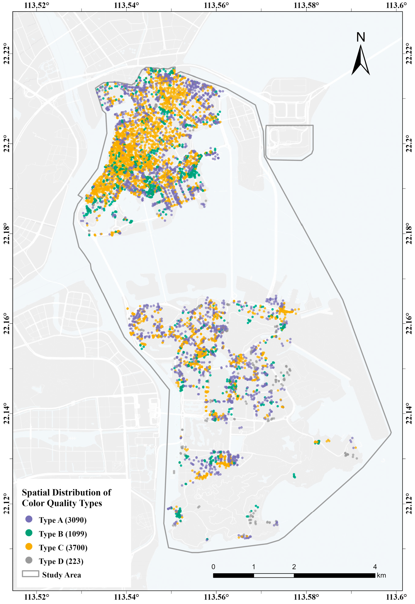
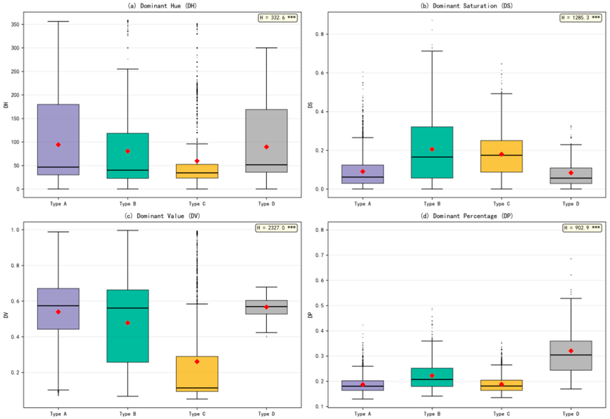
Validation DimensionIndicatorValue
Internal validationSilhouette score0.201
Calinski–Harabasz index1956
Davies–Bouldin index1.420
Consistency validationARI (K-means vs. Ward)0.265
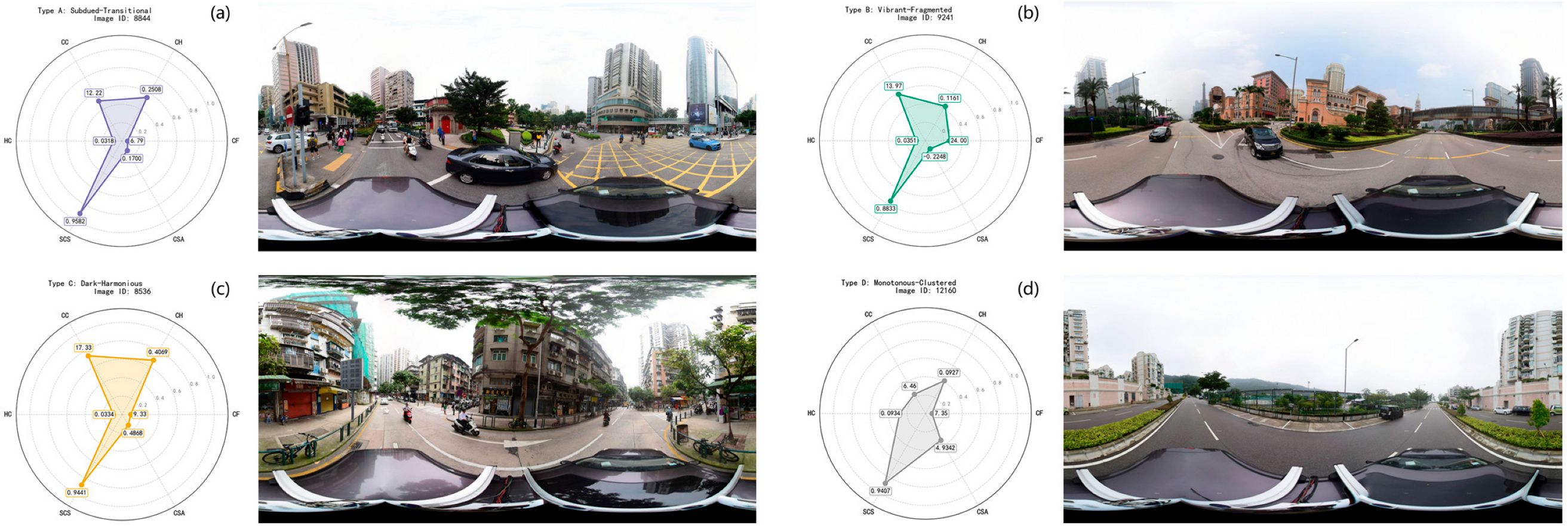
Stability validationMean ARI (50 subsamples)0.968 ± 0.026
Boundary diagnosticPoints with fuzzy membership < 0.693.1%
Table 5. Indicator profiles (mean ± SD) of the four color quality types.
TypenShareCFCHCCHCSCSCSA
Type A309038.1%7.970 ± 4.6000.268 ± 0.08812.920 ± 1.8200.032 ± 0.0130.958 ± 0.0240.340 ± 0.580
Type B109913.5%23.470 ± 11.2000.156 ± 0.16014.790 ± 3.2600.047 ± 0.0210.892 ± 0.0620.230 ± 0.590
Type C370045.6%7.360 ± 4.1500.397 ± 0.09717.270 ± 1.5300.034 ± 0.0140.952 ± 0.0260.370 ± 0.460
Type D2232.7%10.980 ± 7.4800.178 ± 0.1167.270 ± 2.0900.088 ± 0.0420.954 ± 0.0444.630 ± 3.140
Table 6. Differences in F-layer attributes among color quality types.
IndicatorType AType BType CType DTestStatisticp Value
DH (°) a46.740.034.351.4sin/cos K–W b332.6<0.001 ***
DS0.0910.2050.1790.084Kruskal–Wallis1285.3<0.001 ***
DV0.5400.4780.2610.566Kruskal–Wallis2327.0<0.001 ***
DP0.1870.2220.1880.320Kruskal–Wallis902.9<0.001 ***
Note: a DH is a circular variable and is reported as the circular median. b Because the Kruskal–Wallis test is not valid for circular data, DH was decomposed into its sine and cosine components, each tested by Kruskal–Wallis (both p < 0.001). As a parametric corroboration, the Watson–Williams test (circular ANOVA) also indicated significant differences across types (F(3, 8108) = 28.74, p < 0.001); we note, however, that its equal-concentration assumption is only partially satisfied—Types A and D have lower mean resultant lengths (R = 0.378 and 0.432, respectively)—so the sine/cosine test is treated as primary. DS, DV, and DP are linear variables and retain the Kruskal–Wallis test. *** p < 0.001.
Table 7. Indicator values of typical sampling points for each type.
TypeImage NameCFCHCCHCSCSCSA
Type A88446.7930.25112.2230.0320.9580.170
Type B924123.9980.11613.9670.0350.883−0.225
Type C85369.3320.40717.3330.0330.9440.487
Type D121607.3540.0936.4650.0930.9414.934
Disclaimer/Publisher’s Note: The statements, opinions and data contained in all publications are solely those of the individual author(s) and contributor(s) and not of MDPI and/or the editor(s). MDPI and/or the editor(s) disclaim responsibility for any injury to people or property resulting from any ideas, methods, instructions or products referred to in the content.