Predicting the Temperature Regime in Hardening Massive Monolithic Walls Using CatBoost Gradient Boosting

Abstract

Thermal cracking due to hydration heat in massive monolithic walls poses a significant risk, but traditional prediction methods are often too complex for rapid engineering assessments. This study aims to develop machine learning models to predict the maximum temperature and center-to-surface temperature difference in hardening massive walls, considering variable heat exchange, concrete hardening rate, and formwork curing time. A dataset of 855,360 numerical experiments was collected by solving the transient heat conduction equation using the finite element method (FEM), varying wall thickness, initial and ambient temperatures, heat transfer coefficient, hardening rate, curing time, and heat release. CatBoost gradient boosting regression models were trained and validated to predict both output parameters. The models achieved high accuracy with coefficients of determination exceeding 0.99 for both targets, mean absolute percentage errors of 0.2% for maximum temperature and 3% for temperature difference. Feature importance analysis revealed that heat release dominates both predictions (35–43% importance), followed by wall thickness. The developed CatBoost models enable rapid, accurate prediction of thermal regimes in massive monolithic walls without time-consuming finite element simulations, offering a practical tool for assessment of early cracking risk temperature indicators during construction.

1. Introduction

During construction, uneven thermal expansion throughout the volume of massive monolithic structures, caused by the heat of concrete hydration, leads to the development of internal thermal stresses [1]. Thermal cracks form when tensile stresses in the surface layers exceed the ultimate deformability or early tensile strength of concrete [2]. The intensity and nature of early cracking are determined by a combination of factors, including the concrete mix composition, heat exchange conditions with the environment, cement hydration kinetics, and the material’s curing regime. Analytical methods [3,4], simplified engineering techniques reflected in regulatory documents, and numerical modeling [5,6] are used to assess the risk of early cracking.

Simplified methods of current regulatory documents, for example, CIRIA C 766 [7], TCXDVN 305:2004 [8], etc., are based on a very limited number of studies for massive monolithic structures. The reason for this is the lack of data on the dynamics of material behavior in various structures, limited experimental conditions, the difficulty of scaling laboratory results and taking into account temperature processes [9,10].

To select appropriate output parameters for the predictive model, existing regulatory limits should be reviewed. The temperature difference between the core and the surface of concrete (ΔT) is widely recognized as a key factor influencing crack formation in massive monolithic structures [11]. A comprehensive compilation of permissible values for the center-to-surface temperature difference ΔT and the associated temperature gradient ΔT/Δh from various codes and research papers is provided in [12]. The parameters regulated by design codes can be classified into categories: internal temperature gradient; external temperature gradient; absolute temperature. The internal temperature gradient corresponds to the parameter ΔT. The external temperature gradient ΔT_ext is defined as the difference between the maximum temperature in the core and the ambient temperature (core—ambient). The absolute temperature corresponds to the parameter $T_{max}$ and determines the maximum temperature at the center of the structure (core). Each parameter has its own limitations based on the target control function and the type of standardization.

Table 1. Summary of regulatory documents.

Parameter	Threshold Value	Regulatory Document
ΔT, center–surface	15–20 °C	ACI 207.2 R [13], ACI 301-20 [14]
ΔText, core–environment	$\le$25 °C	JASS 5 [16]
$T_{max}$, core	70 °C	ACI 207.2 R [13], ACI 301-20 [14]
ΔText, core–environment	15 °C	DAfStb [15]
ΔT (internal limitation)	20–35 °C	CIRIA C766 [7]

presents a summary of the permissible values for ΔT, ΔT_ext and maximum temperature $T_{max}$ according to the regulations of various countries (ACI [13,14], CIRIA [7], DAfStb [15], and JASS [16]).

An analysis of regulatory documents shows that most temperature requirements are limited to a difference of 15–25 °C between the core and the surface. However, these regulations vary in their degree of conservatism. For example, ACI 207 and ACI 301, based on practical experience in the construction of massive structures, separately regulate the maximum temperature in the core.

To assess temperature stresses $\sigma$ during the construction of massive monolithic structures, dependencies based on the temperature differences $\mathsf{\Delta }T$ are often used [17,18,19,20,21,22]:

$$\sigma ={\displaystyle \frac{k{\alpha }_{T}E\mathsf{\Delta }T}{1+\phi }},$$

(1)

where $E$ is the modulus of elasticity of concrete, ${\alpha }_T$ is the coefficient of thermal expansion, $k$ is the deformation restraint coefficient, and $\phi$ is the creep coefficient of concrete.

Thermal stress assessment is particularly critical in early crack risk analysis, where local temperature and stress extremes can trigger crack initiation [23,24]. Traditional methods for predicting temperature distribution dynamics in hardening massive monolithic walls and slabs, based on numerical modeling using the finite element method [25,26,27,28,29] and analytical approaches [30,31,32], are often labor-intensive and impractical for rapid engineering assessment.

In this regard, machine learning (ML) methods are of particular interest since they are oriented toward working with large databases and are capable of identifying hidden nonlinear relationships between parameters influencing the temperature regime of structures under construction. Studies [33,34] are devoted to predicting the heat of hydration of concrete depending on its composition using machine learning. Article [35] is devoted to the construction of a predictive model for the thermophysical properties of concrete, which is also an important task when assessing the risk of early cracking. Paper [36] uses discrete element method simulations and an AutoML-optimized artificial neural network to show how microscale friction parameters control the macroscopic behavior and failure mode transitions of cementitious composites. Article [37] presents a hybrid predictive model that combines a generalized nearest neighborhood clustering algorithm with a modified particle swarm optimization (PSO) technique to forecast the 28-day compressive strength of pozzolanic concrete used in massive structures. Paper [38] presents an interesting hybrid ML–mechanics framework and discusses strategies for improving model generalizability and the validation of synthetic-data-driven models using self-centering walls as the object of study.

One of the pioneering works aimed at predicting the temperature regime in massive monolithic structures using machine learning is [39]. This publication is devoted to the construction of a predictive model for the quantities $T_{max}$ and $\mathsf{\Delta }T$ in massive monolithic walls during the construction phase. The dataset was generated using the method from CIRIA C766. The training dataset consisted of only 36 records. However, the choice of input variables, such as concrete grade, total binder content, and slag content, implies a high correlation between these parameters, which ultimately leads to multicollinearity in the input variables, incorrect model interpretation, and a distorted representation of the importance of model features. The absence of a parameter determining the concrete hardening rate precludes the cumulative exothermic effect of cement hydration. It should also be noted that the dataset in this study was generated under constant heat exchange conditions on the wall surfaces (wind speed of 5 m/s and 18 mm thick plywood formwork) and a fixed curing time.

The aim of this study is to develop the research direction proposed in [39]. Within the framework of this objective, a machine learning model based on the gradient boosting algorithm (CatBoost) was developed and validated for predicting the temperature regime of hardening massive monolithic walls, taking into account variable heat exchange conditions on the wall surfaces, the rate of concrete hardening, and the curing time of the structure in the formwork. None of these factors were addressed together in previous ML studies for monolithic walls.

2. Materials and Methods

The initial dataset for training the machine learning models was generated through a series of numerical experiments to assess the temperature regime of hardening massive monolithic concrete walls. The numerical modeling was performed taking into account variations in the geometric, thermal, and physical–mechanical parameters of the concrete, as well as environmental conditions, which allowed for the creation of a representative training dataset.

The following were adopted as input parameters for the models: wall thickness $H$ in meters; initial temperature of concrete mix $T_0$ (°C); ambient temperature $T_{\infty }$ (°C); heat transfer coefficient on the side surfaces of the wall $\alpha$ (W/m² °C); concrete hardening rate; curing time in formwork t in days; heat release value at the age of 28 days $Q_{28}$ (MJ/m³). The rate parameter is a categorical variable that takes the values 1 for rapid-hardening, 2 for normal-hardening, and 3 for slow-hardening concrete.

Output parameters were the maximum temperature in the structure, $T_{max}$, and the maximum difference between the center and the surface of the structure, ${∆T}_{max}$, over the whole simulation period. Based on the obtained values of temperature difference ${∆T}_{max}$, an assessment of temperature stresses can then be made using Formula (1). Prediction of the T_max value serves to prevent the risk of delayed ettringite formation during hardening under high temperature conditions.

The heat release function of concrete used to generate the training dataset was defined by an equation in [21]:

$$Q\left(\tau \right)=Q_{28}\exp \left(k\left(1-{\left({\displaystyle \frac{28}{\tau }}\right)}^d\right)\right),$$

(2)

where $\tau$ is the concrete hardening time in days, and the coefficients $k$ and $d$ determine the kinetics of heat release.

The coefficient $k$ value was taken to be 0.14 for rapid-hardening concrete, 0.19 for normal-hardening concrete, and 0.24 for slow-hardening concrete. The coefficient $d$ values were 0.4 for rapid-hardening concrete, 0.51 for normal-hardening concrete, and 0.62 for slow-hardening concrete.

The temperature field was calculated in a simplified one-dimensional formulation using the differential equation:

$$\lambda {\displaystyle \frac{{\partial }^{2}T}{\partial x^2}}+W=\rho c{\displaystyle \frac{\partial T}{\partial \tau }},$$

(3)

where $\lambda$ = 2.67 W/(m·°C) is the thermal conductivity coefficient of concrete, $x$ is the coordinate along the wall thickness ($-H/2\le x\le H/2$), $T$ is the temperature, $W={\displaystyle \frac{\partial Q}{\partial t}}$ is the power of internal heat sources, $\rho$= 2400 kg/m³ is the density of concrete, and $c$ = 1000 J/(kg∙°C) is its specific heat capacity.

The same heat exchange conditions were assumed on the side surfaces of the wall. Due to symmetry, the interval $0\le x\le H/2$ was considered. The boundary conditions at $x=0$ are as follows:

$${\displaystyle \frac{\partial T}{\partial x}}=0.$$

(4)

When $x=H/2$, convective heat exchange takes place with the boundary conditions:

$$\lambda {\displaystyle \frac{\partial T}{\partial x}}+\alpha \left(T-T_{\infty }\right)=0.$$

(5)

Equation (3), with boundary conditions (4) and (5) and the initial condition $T=T_0$, was solved using the finite element method. Euler’s method was used for time integration. Based on the preliminary mesh sensitivity analysis, the number of finite elements across half of the wall thickness was taken to be equal to 20, and the time step was taken to be equal to 1200 s. With further thickening of the finite element mesh and a reduction in the time step, the error in determining temperatures did not exceed 1%. The time step was independent of the coordinate mesh.

The use of a simplified one-dimensional formulation is justified by the fact that for flat structures such as slabs and walls, the temperature distribution, except at the edges, is one-dimensional. The proposed method cannot predict edge effects or the temperature regime of structures with complex shapes.

The calculation method used for dataset formation has been repeatedly tested previously on the experimental data of the authors and other researchers for massive monolithic foundation walls and slabs in the works [40,41,42].

When forming the training dataset, the wall thickness varied from 0.75 to 3 m with a step of 0.25 m (10 different values). The initial temperature of the concrete mix ranged from 5 to 25 °C with a step of 4 °C (6 different values). The lower limit of 5 °C corresponds to the minimum temperature of the concrete mix at the beginning of curing according to Russian standard SR 70.13330.2012 [43]. This same regulatory document also establishes the maximum temperature of the concrete mix for massive structures, which should not exceed 25 °C.

Ambient temperature varied from 5 to 30 °C with a step of 5 °C (6 different values). Neither winter conditions nor conditions of an extremely hot climate were considered since such conditions have their own specifics. For example, for conditions of extremely hot climates, direct supply of liquid nitrogen into the tanks of concrete mixers has recently been carried out to reduce the initial temperature of the concrete mix [44].

The heat transfer coefficient on the side surfaces took values from 1 to 23 W/(m²·°C) with a step of 2 W/(m²·°C) (12 different values). The curing time in the formwork varied from 2 to 12 days with a step of 2 days (11 different values). The removal of the formwork was modeled by changing the heat transfer coefficient α in Formula (5) to a value of 23 W/(m²·°C), which corresponds to an uncovered surface according to the design codes SR 23-101-2004 [45].

The value $Q_{28}$ took values from 50 to 250 MJ/m ³ with a step of 40 MJ/m³ (6 different values). Thus, all input parameters were uniformly distributed. The data volume amounted to 10 × 6 × 6 × 12 × 11 × 6 × 3 = 855,360 numerical experiments. The calculation of a large number of options for dataset formation was automated in the MATLAB R2024a environment using parallel computing.

Table 2. Training dataset.

No.	Input Parameters							Output Parameters
	$\mathit{H}$	${\mathit{T}}_0$	${\mathit{T}}_{\mathit{\infty }}$	$\mathit{\alpha }$	Rate	$\mathit{t}$	${\mathit{Q}}_{28}$	${\mathit{T}}_{\mathit{m}\mathit{a}\mathit{x}}$	${∆\mathit{T}}_{\mathit{m}\mathit{a}\mathit{x}}$
1	0.75	5	5	1	1	2	50	18.98621925	8.008572674
2	0.75	5	5	1	1	2	90	30.17519466	14.41543081
3	0.75	5	5	1	1	2	130	41.36417006	20.82228895
4	0.75	5	5	1	1	2	170	52.55314546	27.22914709
5	0.75	5	5	1	1	2	210	63.74212087	33.63600523
6	0.75	5	5	1	1	2	250	74.93109627	40.04286337
7	0.75	5	5	1	1	3	50	18.98708877	7.810228113
8	0.75	5	5	1	1	3	90	30.17675978	14.0584106
9	0.75	5	5	1	1	3	130	41.36643079	20.30659309
10	0.75	5	5	1	1	3	170	52.55610181	26.55477558
11	0.75	5	5	1	1	3	210	63.74577282	32.80295807
12	0.75	5	5	1	1	3	250	74.93544383	39.05114056
13	0.75	5	5	1	1	4	50	18.98708877	7.457900342
…	…	…	…	…	…	…	…	…	…
344,830	1.75	5	10	3	2	9	130	40.27157644	18.96434837
344,831	1.75	5	10	3	2	9	170	50.74915088	25.33648985
344,832	1.75	5	10	3	2	9	210	61.23282274	31.70863132
344,833	1.75	5	10	3	2	9	250	71.71962171	38.0807728
344,834	1.75	5	10	3	2	10	50	19.40120632	5.910121918
344,835	1.75	5	10	3	2	10	90	29.80880729	11.90767519
344,836	1.75	5	10	3	2	10	130	40.27157644	17.90540647
…	…	…	…	…	…	…	…	…	…
855,352	3	25	30	23	3	11	170	69.21754625	33.85300796
855,353	3	25	30	23	3	11	210	79.23781157	42.50103214
855,354	3	25	30	23	3	11	250	89.26206596	51.15247135
855,355	3	25	30	23	3	12	50	39.28364502	8.017428934
855,356	3	25	30	23	3	12	90	49.21107241	16.58605506
855,357	3	25	30	23	3	12	130	59.20502956	25.21160309
855,358	3	25	30	23	3	12	170	69.21754625	33.85300796
855,359	3	25	30	23	3	12	210	79.23781157	42.50103214
855,360	3	25	30	23	3	12	250	89.26206596	51.15247135

partially shows the analyzed dataset.

Statistical characteristics of the initial data and assessments of their distributions were carried out using descriptive statistics (

Table 3. Statistical characteristics of the dataset.

	$\mathit{H}$	${\mathit{T}}_0$	${\mathit{T}}_{\mathit{\infty }}$	$\mathit{\alpha }$	Rate	$\mathit{t}$	${\mathit{Q}}_{28}$	${\mathit{T}}_{\mathit{m}\mathit{a}\mathit{x}}$	${∆\mathit{T}}_{\mathit{m}\mathit{a}\mathit{x}}$
mean	1.88	15.00	17.50	12.0	2.00	7.00	150.00	51.91	24.56
std	0.72	6.83	8.54	6.9	0.82	3.16	68.31	19.50	15.65
min	0.75	5.00	5.00	1.0	1.00	2.00	50.00	8.97	0.52
25%	1.25	9.00	10.00	6.5	1.00	4.00	90.00	36.18	11.74
50%	1.88	15.00	17.50	12.0	2.00	7.00	150.00	49.59	21.40
75%	2.50	21.00	25.00	17.5	3.00	10.00	210.00	65.86	34.74
max	3.00	25.00	30.00	23.0	3.00	12.00	250.00	113.76	90.30

).

To quantitatively confirm deviations of the parameter distributions from the normal distribution law for $T_{max}$ and ${∆T}_{max}$, the Shapiro–Wilk test was used. Standard statistical packages such as SciPy (v1.0.0 and higher), R (v4.6.0), and IBM SPSS v32 use this test by default. In our case, its use is obvious for several reasons: first, it is designed for large sample sizes (n = 855,360); second, a random subsample of 5000 samples is used to ensure the test is valid. In addition, the Shapiro–Wilk test is easy to interpret. At a p-value > 0.05, there is no reason to reject the hypothesis of a normal distribution.

Machine learning models based on decision trees were selected to solve the problem. CatBoost Regression (CatBoostRegressor) was chosen due to its robustness to multicollinearity, ability to model nonlinear relationships, and high forecasting accuracy. The choice of the CatBoost algorithm was also justified by its ability to handle categorical features without preprocessing. Our dataset includes a categorical variable, rate (concrete hardening rate: rapid, normal, or slow). CatBoost, unlike XGBoost, LightGBM, Support Vector Regression and Artificial Neural Networks, processes categorical features using target-based encoding and ordered boosting. This eliminates the risk of data leakage associated with naive one-hot encoding and improves model quality.

Range selection for grid search with five-fold cross-validation as applied to CatBoostRegressor was defined as follows: iterations {500, 1000, 1500}; learning_rate {0.05, 0.1}; depth {4, 6}. Additionally, parameters with fixed values were used: random_seed = 42; subsample = 0.8.

To assess the quality and stability of the constructed forecasting models, graphs of residuals over time were constructed for the components $T_{max}$ and ${∆T}_{max}$.

3. Results

Based on the results of the primary analysis of the source data and descriptive statistics, a table of numerical characteristics of the target variables was compiled for $T_{max}$ and ${∆T}_{max}$ (

Table 4. Indicators of the distribution form for target variables.

Parameter	Sample Size	Asymmetry (Skewness ${\mathit{\gamma }}_1$)	Excess (Kurtosis ${\mathit{\gamma }}_2$)	p-Value (Shapiro–Wilk)	Distribution Pattern
$T_{max}$	855,360	0.4113	−0.5710	4.04 × 10−29	Moderately right-sided asymmetry, flat-topped (platykurtic)
${∆T}_{max}$	855,360	0.7601	−0.0684	5.82 × 10−42	Marked right-sided asymmetry, close to normal (mesokurtic)

).

According to the Shapiro–Wilk criterion, the distributions of the target variables $T_{max}$ and ${∆T}_{max}$ (Table 4) statistically significantly deviate from normal (p-value < 10⁻²⁸).

Based on the indicators of the distribution shape for the target variables, it can be concluded that there is a positive asymmetry and a negative excess, both for $T_{max} ({\gamma }_1=0.41; {\gamma }_2=-0.57)$ and ${∆T}_{max} ({\gamma }_1=0.76; {\gamma }_2=-0.06)$.

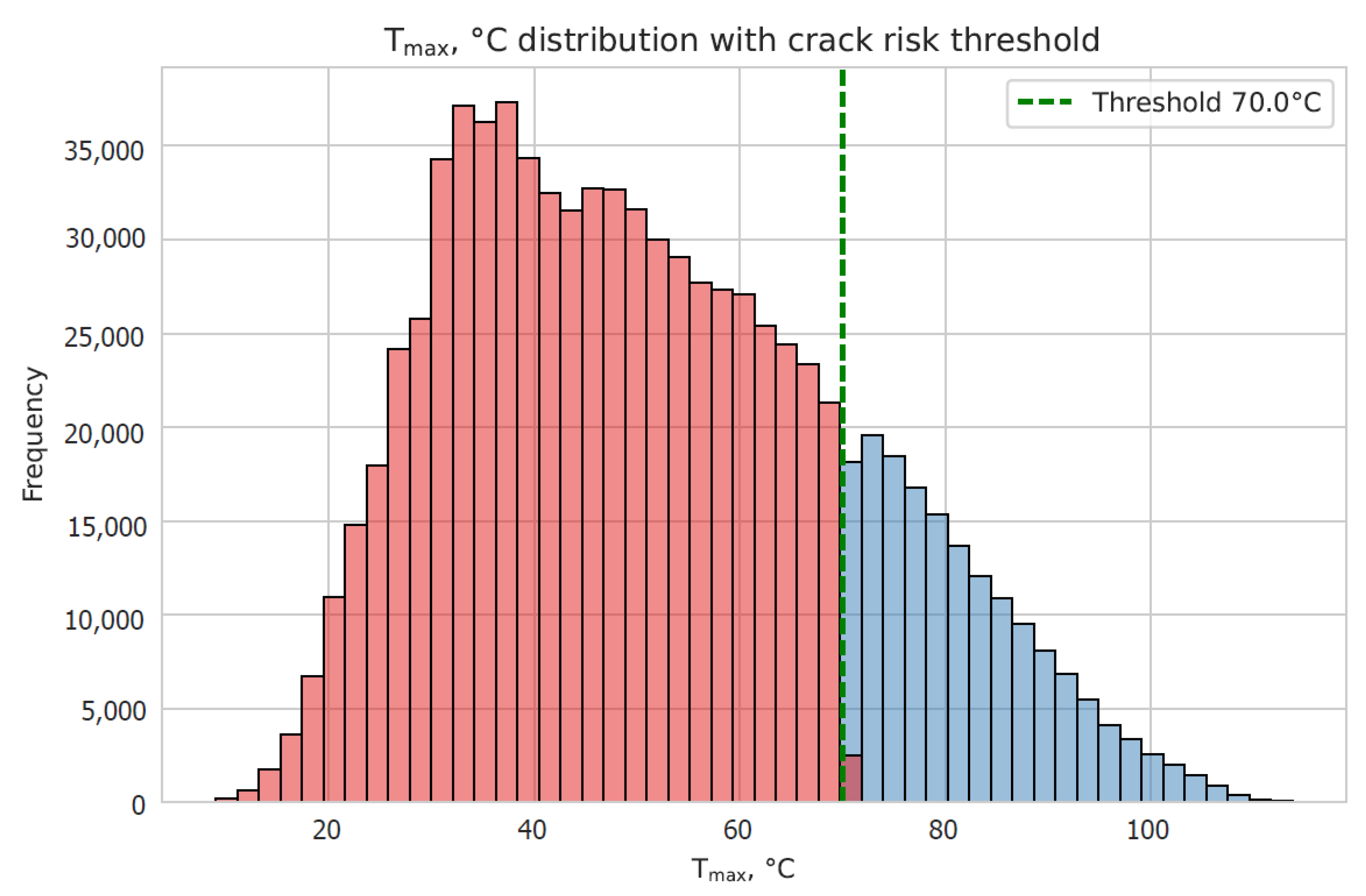
A $T_{max}$ distribution histogram for the entire dataset is presented in Figure 1. The graph shows values $T_{max}$ in the range of 20–100 °C along the OX-axis. The frequency of occurrence is shown along the OY-axis.

The boundary value $T_{max}=70 °\mathrm{C}$ divides the sample into two areas, zones of permissible temperatures and zones of exceeding regulatory limits, characterized by an increased probability of the development of destructive processes, including reactions of delayed ettringite formation.

The distribution has a multimodal character (the presence of several peaks). The majority of observations are concentrated in the temperature range below the threshold, which corresponds to safe curing conditions. However, a significant proportion of cases exceed $T_{max}\ge$ 70 °C and form the right tail of the distribution, indicating potentially hazardous scenarios associated with high heat generation and large structural thicknesses.

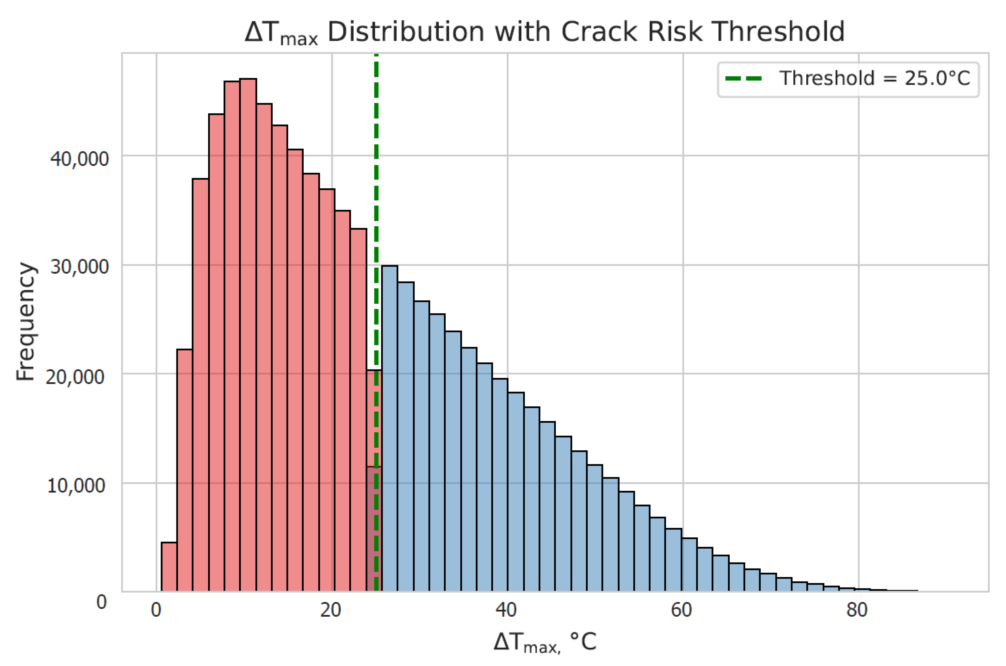
The distribution histogram of the maximum difference between the center and surface of the structure for the entire dataset is shown in Figure 2. The horizontal axis represents data ${∆T}_{max}$ in a range from 0 °C to 80 °C, and the vertical axis represents the frequency of occurrence from 0 to 40,000. The distribution pattern is bimodal (there are two characteristic peaks). The threshold ${∆T}_{max}$ = 25 °C is indicated on the graph by a vertical dotted line, as in the case for $T_{max}$. The choice of a single threshold value of 25 °C for ΔT_max is not intended to represent a universal international requirement. It serves as a conservative screening criterion for visual differentiation of the bimodal distribution into two zones. This value lies within the range of recommendations given in ACI (15–20 °C) and CIRIA (20–35 °C). Using this threshold allows for unambiguous separation of scenarios into safe and hazardous zones.

For the ${∆T}_{max}$ parameter, the first clearly defined peak is observed at ${∆T}_{max}\approx$ 10–15 °C (safe zone). The second peak is observed at ${∆T}_{max}\approx$ 25–30 °C, corresponding to the zone of relative risk uncertainty.

The obtained distributions (Figure 1 and Figure 2) emphasize the need for forecasting $T_{max}$ and ${∆T}_{max}$, as well as the application of controlled technological measures to reduce the risk of early cracking in massive monolithic structures.

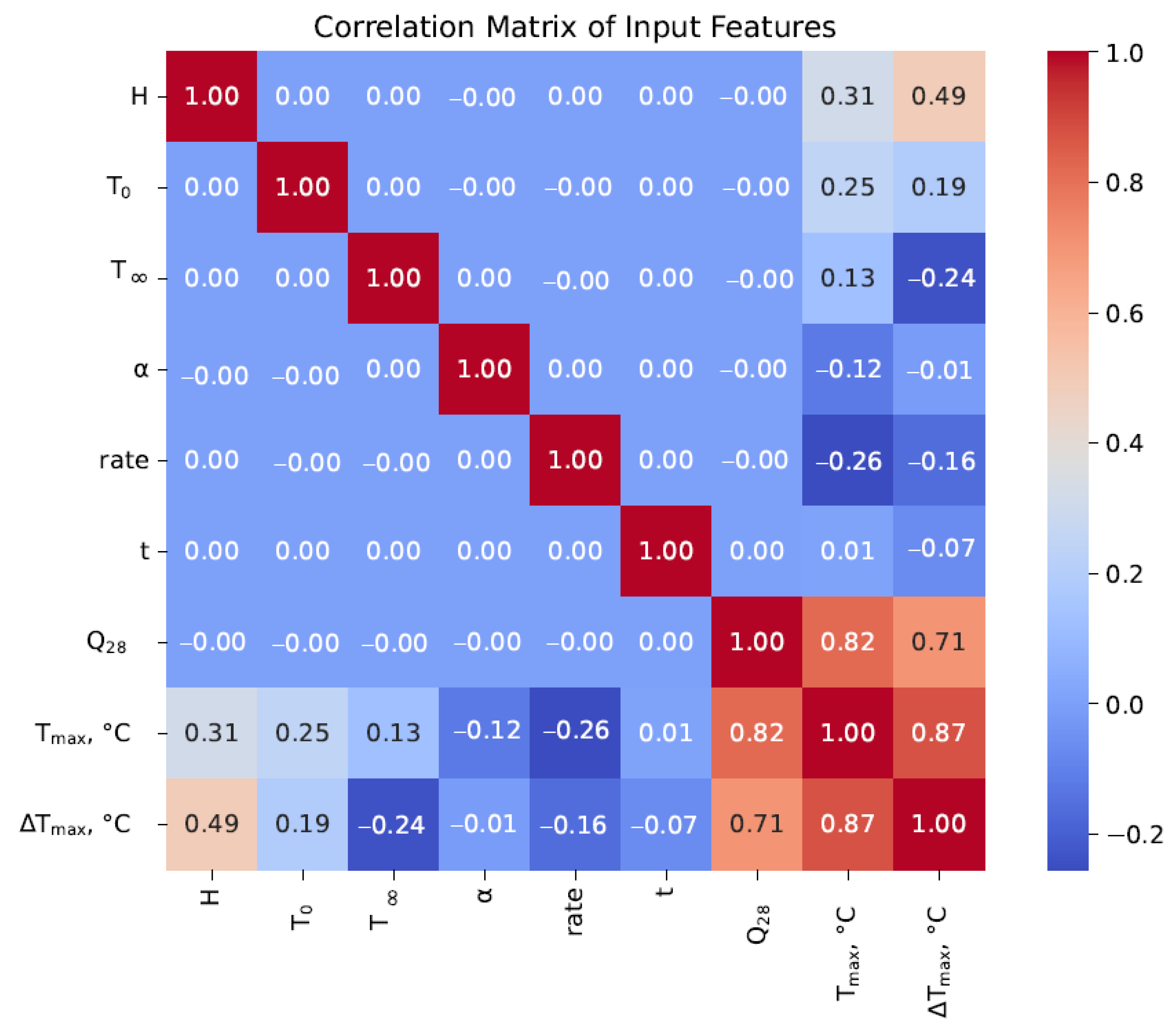
Figure 3 shows a heat map of the correlation matrix of the input and target variables. All input parameters are independent of each other (zero correlation coefficients), which is due to the algorithm used to generate a synthetic dataset (a full-factorial dataset).

The analysis revealed a strong positive correlation between the parameters $Q_{28}$ and $T_{max}$ (${\rho }_{Q_{28}/T_{max}}=0.82$) and between $Q_{28}$ and $\mathsf{\Delta }{T}_{max}$ (${\rho }_{Q_{28}/{\mathsf{\Delta }T}_{max}}=0.71$). This is expected since the high heat release of cement leads to an increase in the maximum temperature in the structure, as well as the temperature difference between the core and the surface.

A strong positive relationship exists between the output parameters $T_{max}$ and $\mathsf{\Delta }{T}_{max}$ (${\rho }_{T_{max}/{\mathsf{\Delta }T}_{max}}=0.87$). Intense concrete heat release is accompanied by an increase in both the maximum core temperature and the temperature difference between the center and surface of the structure.

The moderate correlation between parameters $H$ and $\mathsf{\Delta }{T}_{max}$ (${\rho }_{H/{\mathsf{\Delta }T}_{max}}=0.49$), as well as between $H$ and $T_{max}$ (${\rho }_{H/T_{max}}=0.31$), is due to the fact that increasing the structural massiveness hinders the dissipation of the released hydration heat. The remaining parameters show a weak or near-zero correlation. The least significant effect on the output parameters, in terms of correlation analysis, is the time the structure is cured in the formwork (${\rho }_{t/T_{max}}=0.01$; ${\rho }_{t/\mathsf{\Delta }{T}_{max}}=-0.07$). This is explained by the fact that the greatest temperature gradients and temperature differences typically develop in the first three days, while the structure is still in the formwork.

In preliminary experiments, we compared CatBoost with XGBoost, LightGBM, and Random Forest. CatBoost demonstrated the best combination of metrics: minimal MAPE (0.2% for T_max and 3% for ΔT_max) with the highest coefficient of determination (R² > 0.99), as well as the smallest error variance on the test data. This allowed us to settle on CatBoost without increasing the ensemble complexity. The forecast quality metrics for CatBoost, XGBoost, LightGBM, and Random Forest are presented in

Table 5. Forecast quality metrics.

Model	Target Variable	R2	RMSE	MAPE (%)	Training Time (s)	Inference Time (ms/Sample)
CatBoost	$T_{max}$	0.999	0.167	0.20	1180	0.12
	$\mathsf{\Delta }{T}_{max}$	0.998	0.581	3.0	1220	0.12
XGBoost	$T_{max}$	0.991	0.258	0.31	830	0.09
	$\mathsf{\Delta }{T}_{max}$	0.989	0.842	4.3	850	0.09
LightGBM	$T_{max}$	0.989	0.274	0.33	710	0.08
	$\mathsf{\Delta }{T}_{max}$	0.986	0.917	4.6	730	0.08
Random Forest	$T_{max}$	0.972	0.515	0.68	1950	0.35
	$\mathsf{\Delta }{T}_{max}$	0.958	1.375	7.1	2010	0.35

. Training and inference times are given for the following setup: Intel Xeon Gold 6240, 64 GB RAM, single-threaded mode. These values are illustrative for ensembles of comparable complexity (500 trees for all algorithms except RF; 300 trees for acceptable times using RF). The comparison was based on a single training protocol without repeated runs or statistical significance testing. As a result, the reported superiority of CatBoost should be interpreted cautiously.

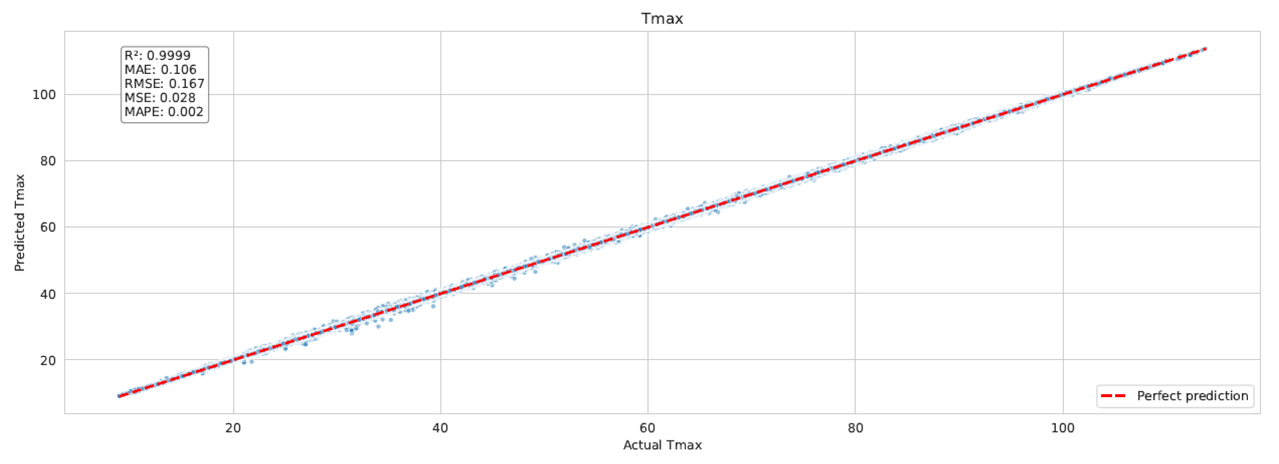
Figure 4 shows a comparison of actual and predicted maximum temperature values $T_{max}$ (°C) for the CatBoost model. The abscissa axis represents temperature intervals from 10 to 100 °C, and the ordinate axis represents the corresponding model forecasts. The red dotted line indicates the ideal match between the forecast and actual values.

The scatter of the points indicates the homoscedasticity of the residuals: the magnitude of the scatter does not increase either in the region of low temperatures (10–30 °C) or in the region of high $T_{max}$ values (70–100 °C). This fact is especially important since it is in this range that the probability of ettringite formation is high.

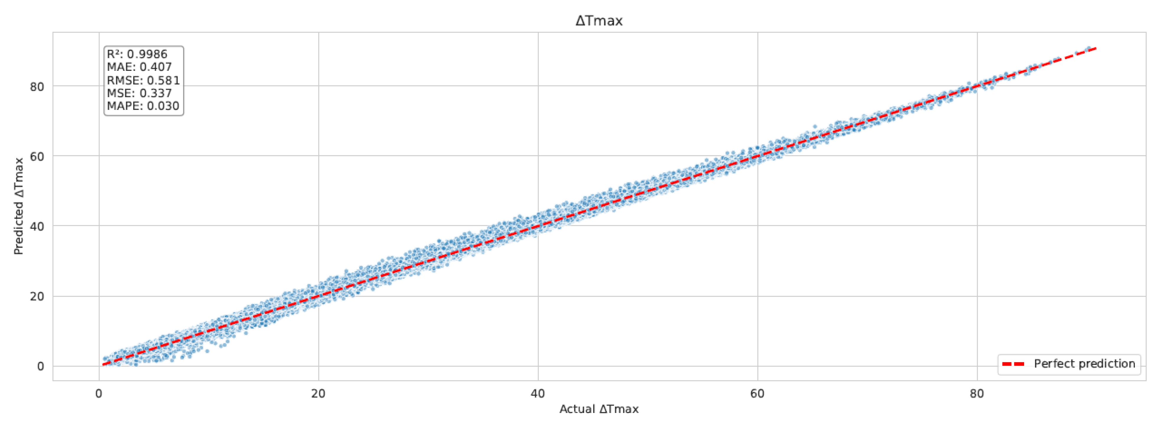
Figure 5 shows a comparison of actual and predicted values for the ${∆T}_{max}$ model (°C). The graph shows no significant shifts, suggesting that the model is robust.

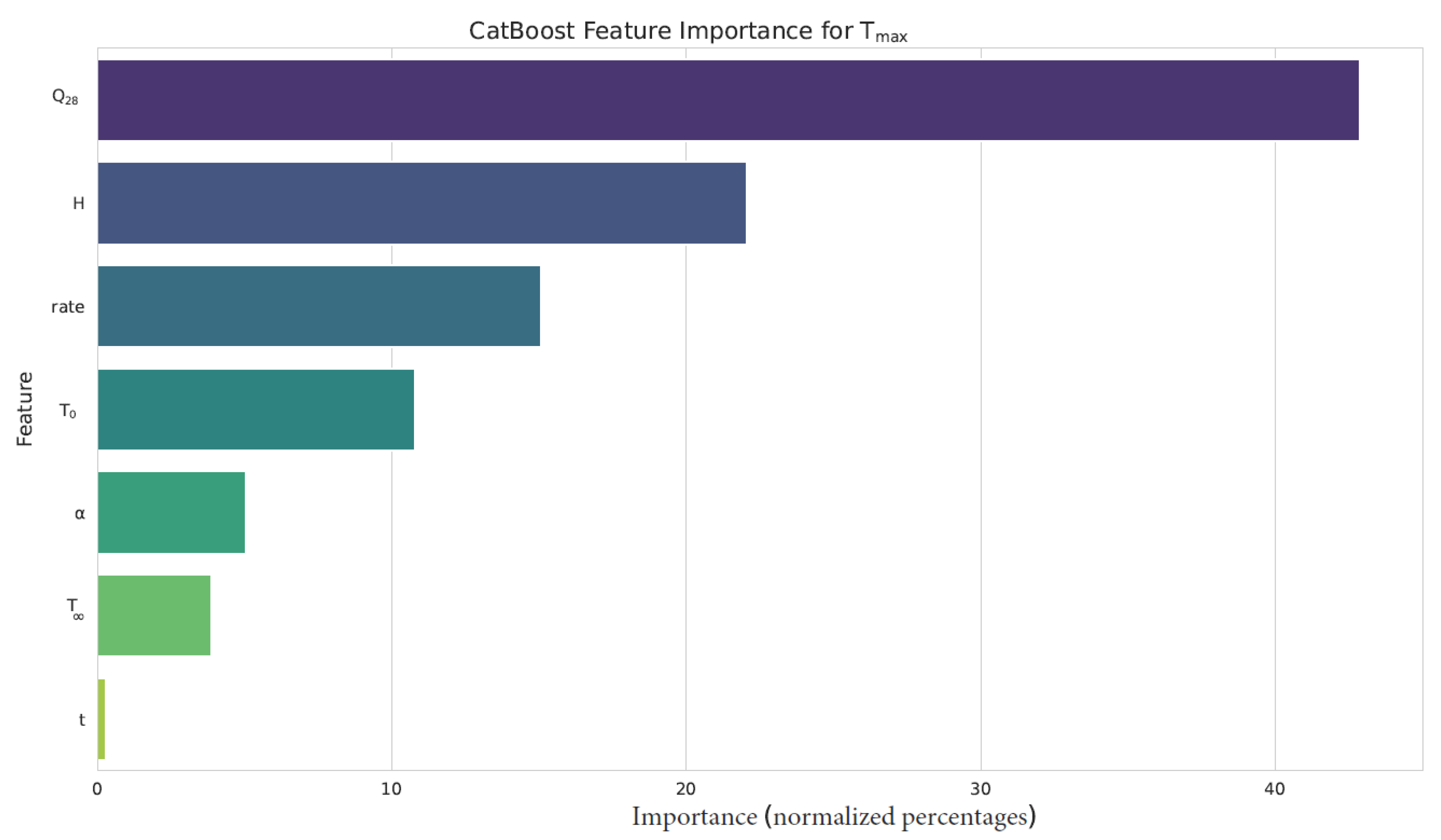
The feature importance analysis of the $T_{max}$ model used to predict the maximum temperature in a massive monolithic wall is presented in Figure 6.

The degree of participation and quantitative assessment of the model parameters are as follows: $Q_{28}$—42.9% (raw score = 95); $H$—22.1% (raw score = 48); rate—15.1% (raw score = 33); $T_0$—10.8% (raw score = 22); $\alpha$—5.1% (raw score = 11); $T_{\infty }$—3.9 (raw score = 7); $t$—0.3% (raw score = 0.7).

Analysis shows that the greatest influence on the forecast is the heat release of concrete $Q_{28}$, significantly outweighing other parameters. The second most important factor is the wall thickness $H$, which determines the structure’s ability to accumulate and dissipate heat. The hardening rate, which reflects the kinetics of cement hydration, also has a significant impact.

The initial concrete temperature $T_0$ makes a moderate contribution to the maximum temperature, while the heat transfer coefficient $\alpha$ and ambient temperature $T_{\infty }$ have a secondary effect. The parameter of curing time in the formwork $t$ has minimal significance, which is consistent with the results of the previous correlation analysis.

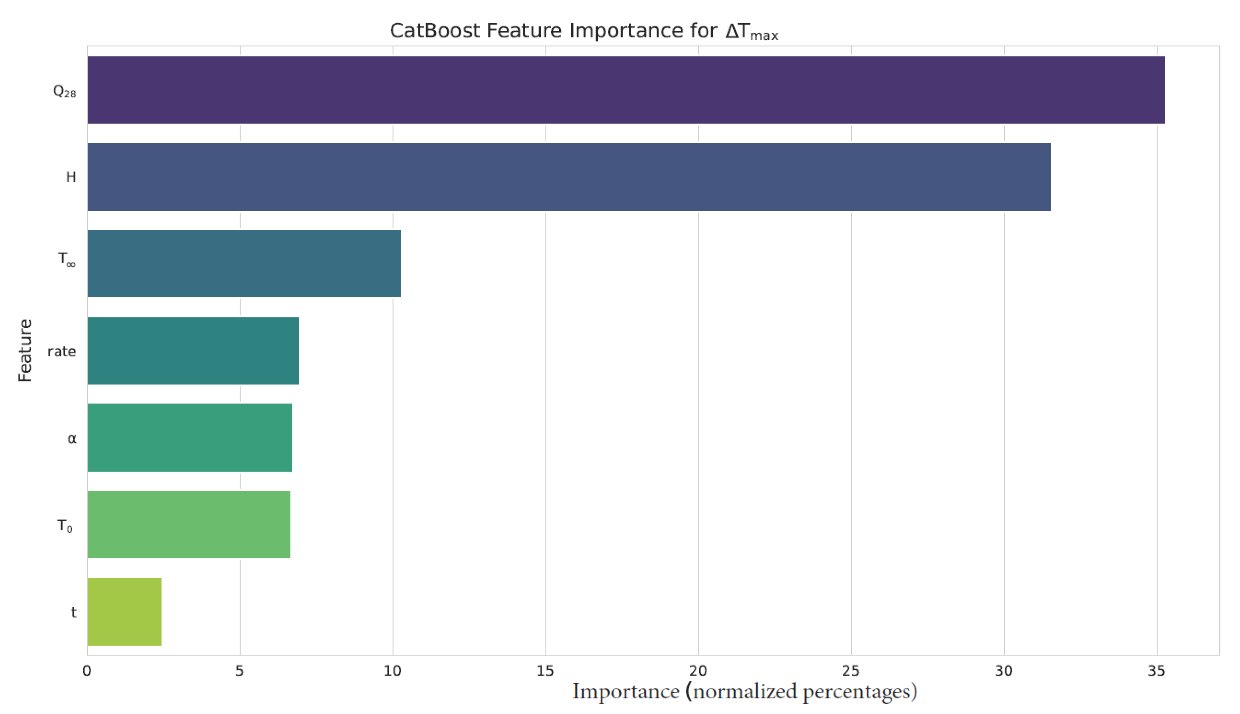
An analysis of the feature importance for the model, ${∆T}_{max}$, used to predict the maximum temperature difference in a massive monolithic wall is presented in Figure 7.

The degree of participation and quantitative assessment of the model parameters are as follows: $Q_{28}$—35.3% (raw score = 94); $H$—31.6% (raw score = 84); $T_{\infty }$—10.3% (raw score = 27); rate—7% (raw score = 19); $\alpha$—6.7% (raw score = 18); $T_0$—6.7% (raw score = 18); $t$—2.5% (raw score = 5).

The greatest contribution to ${∆T}_{max}$ formation is made by the heat release of concrete $Q_{28}$, emphasizing the crucial role of exothermic hydration in the development of temperature gradients. Wall thickness $H$ also has a significant influence, determining the conditions of heat accumulation and the intensity of its dissipation. The remaining model parameters contribute moderately or very little to the predicted values, such as the curing time in the formwork $t$. It should be noted that feature importance reflects predictive contribution within the considered parameter space rather than absolute physical causation.

During model training, the best parameter values were obtained for the CatBoostRegressor models, which are presented in

Table 6. Optimal parameter values for CatBoostRegressor models.

No.	Parameter/Model	${\mathit{T}}_{\mathit{m}\mathit{a}\mathit{x}}$	${∆\mathit{T}}_{\mathit{m}\mathit{a}\mathit{x}}$
1	depth	6	6
2	learning_rate	0.05	0.05
3	iterations	1000	1000
4	random_seed	42	42
5	subsample	0.8	0.8

.

A grid search resulted in several excellent combinations: depths of 4 and 6; learning rates of 0.05 and 0.1; and iterations of 1000. The minimum error was achieved with a depth of 6, a learning rate of 0.05, and a fixed iteration count of 1000. The obtained results not only confirm the quality of the constructed model but also reveal physically based dependencies.

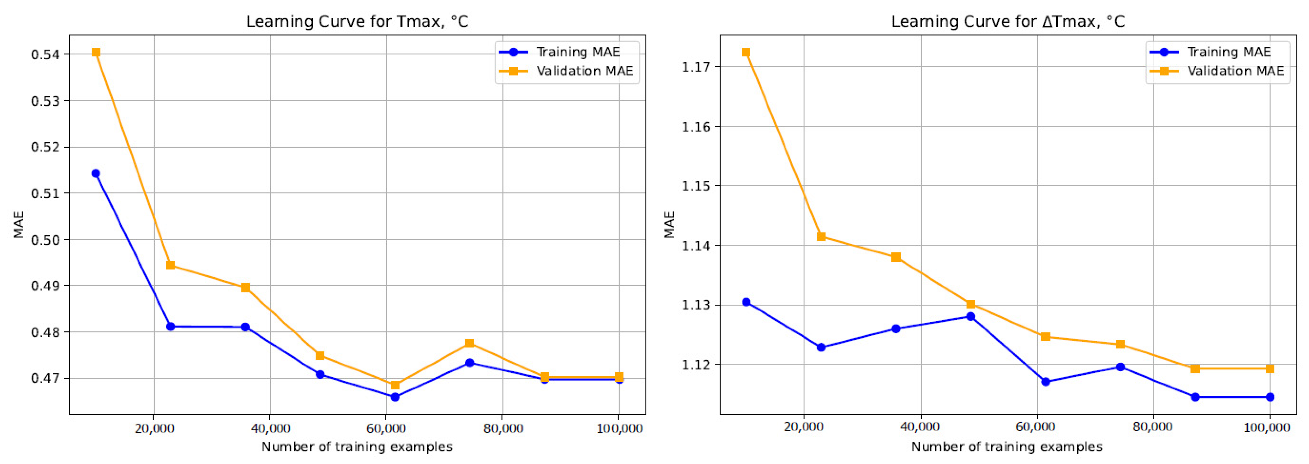
To assess the impact of sample size on the forecasting performance of models, a learning curve analysis was conducted. A visual representation of the results is presented in the learning curve graphs for $T_{max}$ and ${∆T}_{max}$ (Figure 8). Both CatBoostRegressor models demonstrated robust learning without overfitting and reached the limit of their predictive power with a training sample size of approximately 60,000–80,000 records.

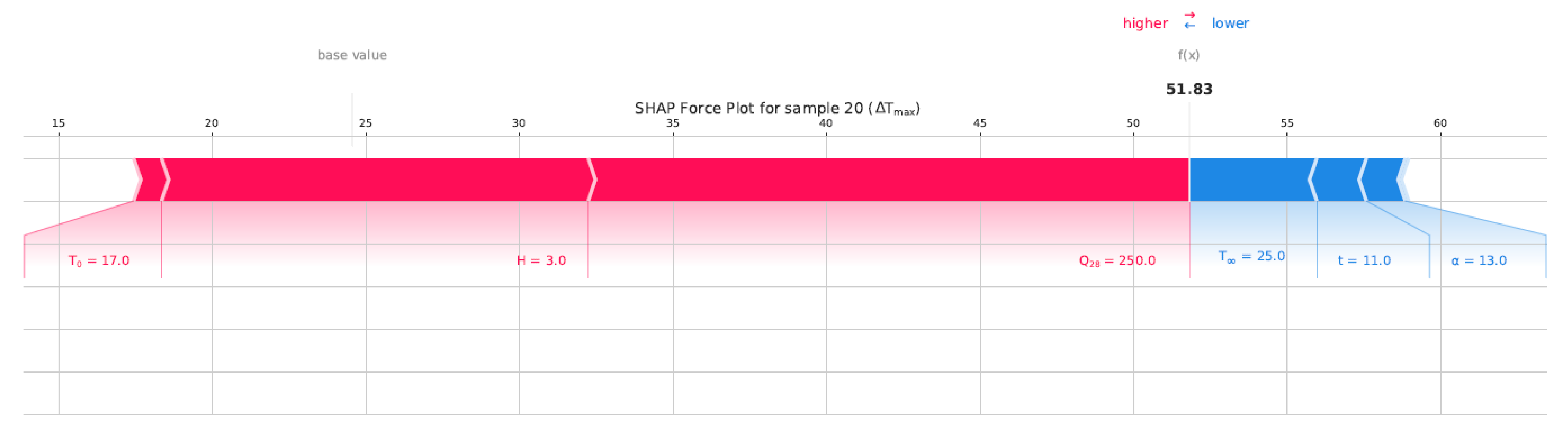
Figure 9 shows a numerical experiment for the specific sample corresponding to a certain case or scenario, be it a climate scenario, hazardous or safe in terms of the risk period for cracking in massive foundation walls. The SHAP (SHapley Additive exPlanations) method was used for the analysis of the data from the following sample record: $H=3$m; $T_0=17$°C; $T_{\infty }=25$ °C; $\alpha =13$ W/(m²·°C); $t=11$ days; $Q_{28}=250$MJ/m³.

Basic elements of the graph are:

−

Base value—the average forecast of the model for the entire training sample;

−

The final prediction $f\left(x\right)$ is the value that the model produced for a given sample.

Color stripes:

−

Red bars mean that the features push the forecast towards an increase (to the right, “higher”);

−

The blue stripes push in the direction of decrease (to the left, “lower“);

−

The length of the stripe is proportional to the SHAP value (feature contribution).

Based on the SHAP analysis of the force plot for the specific observation, the following interpretation of the model for ${∆T}_{max}$ predictions can be made:

• Very high exothermicity leads to intense heating of the wall’s center, which sharply increases the temperature difference between the center and the surface of the wall, which is physically justified. The longest red segment corresponds to $Q_{28}=250$MJ/m³.
• A massive wall dissipates heat less effectively, accumulating it in the center, which further increases the temperature difference. The second longest red segment is H = 3 m.
• Ambient temperature $T_{\infty }=25$ °C (moderate) and initial temperature $T_0=17$°C (low) somewhat reduce the gradient, but their contribution is less than that of $Q_{28}$ and H. The logic is that higher $T_{\infty }$ reduces surface cooling. For the ${∆T}_{max}$ model, the higher the $T_{\infty }$, the smaller the difference (the surface does not cool significantly). $T_0=17$ °C is below the baseline, so its contribution can be negative. The blue bars reflect a moderate impact on the model’s predicted values.
• The curing time in the formwork is $t=11$ days. By this point in time, the peak of exothermicity has already passed; accordingly, the temperature difference between the center and the surface of the structure decreases compared to the first day, which gives a negative contribution (blue bar).
• The heat transfer coefficient $\alpha =13$ W/(m²·°C) helps equalize the temperature, reducing the difference.

Total forecast is ${∆T}_{max}\approx 45–50 °\mathrm{C}$. This is very high, since for massive concrete structures, a temperature difference of more than 20–25 °C is already considered risky in terms of thermal cracking. In this case, the difference is almost twice the critical threshold.

The main indicators are the extremely high exothermicity of the cement ($Q_{28}=250$MJ/m³) and the large wall thickness (H = 3 m). Even at moderate initial temperatures and conditions, the model, ${∆T}_{max}$, predicts dangerous stress levels.

4. Discussion

An analysis of the feature importance suggests that the most effective way to reduce ΔT_max is to reduce the heat release of concrete (Q₂₈) and/or to reduce the wall thickness. If the thickness is determined by the design, the primary control mechanism is to select a concrete composition with reduced exothermicity (e.g., with the addition of ash or slag). Varying the heat transfer coefficient α (e.g., by insulating the formwork) has a secondary effect: for α, from 1 to 23 W/(m²·°C), the contribution to the model is only 5–7%. This means that attempts to control cracking solely through surface insulation with high cement exothermicity are ineffective—reducing the heat release itself is the key measure.

The trained models were also tested on independent numerical data presented in [39]. As mentioned earlier, in that work, the training dataset included 36 samples. The input variables were the wall thickness (0.5, 1 and 1.5 m), the type of cement (CEM I, CEM I + 30% slag and CEM I + 60% slag), the binder consumption (340 and 380 kg/m³), the initial temperature of the concrete mix (15 and 30 °C), and the ambient temperature (10 and 25 °C). Heat exchange conditions on the surfaces were assumed to be constant (a formwork made of 18 mm thick plywood at a wind speed of 5 m/s).

For comparison with the results of [39], the specific heat release of cement at the age of 28 days was taken to be equal to 380.3 kJ/kg for CEM I, 311.8 kJ/kg for CEM I + 30% slag and 243.4 kJ/kg for CEM I + 60% slag.

The heat transfer coefficient with uncovered surfaces, ${\alpha }_{open}$, depending on the wind speed, $v$, was determined using the following formula [46]:

$${\alpha }_{open}=6+3.7v=24.5 \mathrm{W}/({\mathrm{m}}^2·°\mathrm{C})$$

(6)

The heat transfer coefficient from the surface covered with formwork, with a thickness $\delta$ of 18 mm and a thermal conductivity coefficient of plywood of $\lambda =0.18$ W/(m·°C), was:

$${\alpha }_f={\displaystyle \frac{1}{\frac{\delta }{{\lambda }_f}+\frac{1}{{\alpha }_{open}}}}={\displaystyle \frac{1}{\frac{0.018}{0.18}+\frac{1}{24.5}}}=7.1 \mathrm{W}/({\mathrm{m}}^2·°\mathrm{C})$$

(7)

The curing time in formwork for all samples was taken to be 7 days, and the hardening rate was rapid-hardening.

Table 7. Comparison of the results obtained by the authors with the data of [39].

H, m	T0, °C	T∞, °C	Q28, MJ/m3	Tmax, [39]	∆Tmax, [39]	Tmax, Authors	∆Tmax, Authors
0.5	15	10	129.30	40	5.6	38.23	7.54
0.5	30	25	129.30	63.7	7.3	53.47	7.44
0.5	15	10	106.01	33.3	4.4	33.90	6.32
0.5	30	25	106.01	58	6.2	49.06	6.28
0.5	15	10	82.76	27.1	3.2	29.69	5.12
0.5	30	25	82.76	50.9	4.9	44.71	5.15
1	15	10	129.30	51.4	13	45.28	13.96
1	30	25	129.30	72.3	14.7	60.34	13.73
1	15	10	106.01	44	10.7	39.72	11.66
1	30	25	106.01	67.1	13.1	54.72	11.50
1	15	10	82.76	35.8	8.1	34.24	9.42
1	30	25	82.76	59.2	10.7	49.15	9.35
1.5	15	10	129.30	57.8	19.2	49.85	19.40
1.5	30	25	129.30	76.1	20.1	64.80	19.13
1.5	15	10	106.01	50.8	16.5	43.47	16.25
1.5	30	25	106.01	71.6	18.5	58.38	16.00
1.5	15	10	82.76	41.8	13	37.18	13.18
1.5	30	25	82.76	63.8	15.5	51.98	13.01
0.5	15	10	144.51	43.1	6.2	41.11	8.35
0.5	30	25	144.51	68	8.1	56.34	8.22
0.5	15	10	118.48	35.8	4.9	36.20	6.97
0.5	30	25	118.48	61.6	6.9	51.42	6.90
0.5	15	10	92.49	28.9	3.6	31.45	5.63
0.5	30	25	92.49	53.7	5.4	46.51	5.62
1	15	10	144.51	55.8	14.4	48.96	15.49
1	30	25	144.51	77.6	16.3	63.98	15.24
1	15	10	118.48	47.5	11.8	42.69	12.89
1	30	25	118.48	71.7	14.6	57.73	12.68
1	15	10	92.49	38.4	9	36.53	10.36
1	30	25	92.49	63	11.9	51.47	10.24
1.5	15	10	144.51	62.9	21.3	54.05	21.50
1.5	30	25	144.51	81.7	22.3	68.97	21.25
1.5	15	10	118.48	55.1	18.3	46.88	17.92
1.5	30	25	118.48	76.7	20.5	61.82	17.66
1.5	15	10	92.49	45.1	14.3	39.81	14.46
1.5	30	25	92.49	68	17.2	54.65	14.24

presents a comparison of the predictions of the model developed by the authors with the results obtained in [39]. The average value of the ratio ∆T₁/∆T₂, where index 1 corresponds to the results of [39] and index 2 corresponds to the authors’ results, was 0.97. The average value of the ratio T_max1/T_max2 was 1.14.

It should be noted that in [39], the dataset was constructed using a simplified method from CIRIA C 766, and we directly solved the differential heat conduction equation, which is more accurate than the simplified method. It has led to an average deviation of 14% in the maximum temperature in the middle of the thickness. It is also important to consider that cements from different manufacturers may differ in heat release. We used the average data for the CEM I cements of Russian producers [47].

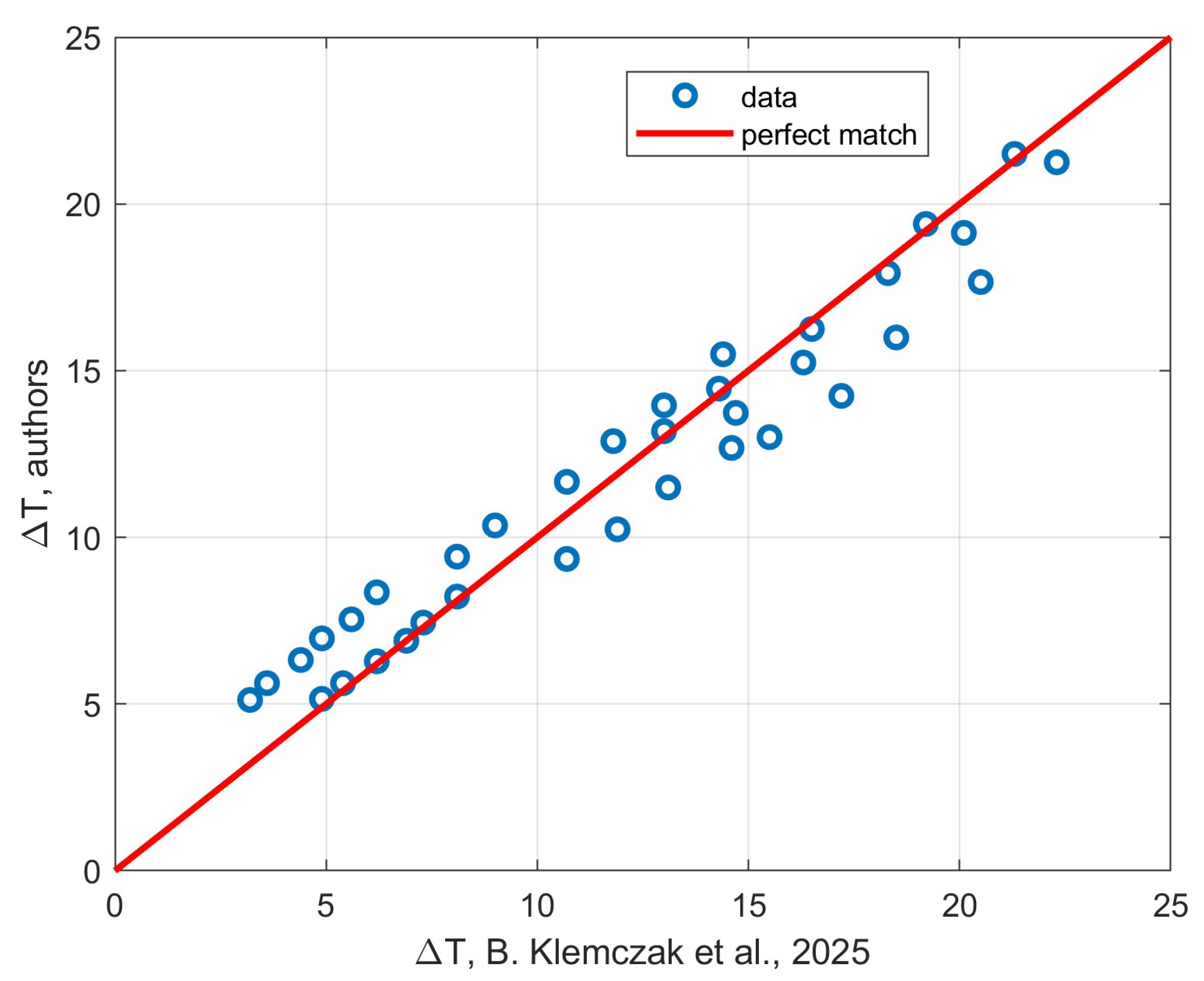
At the same time, the CIRIA method C 766 predicts the maximum center-to-surface temperature difference quite well. A visual comparison of the results obtained in [39] with the authors’ solution for the maximum temperature difference is shown in Figure 10.

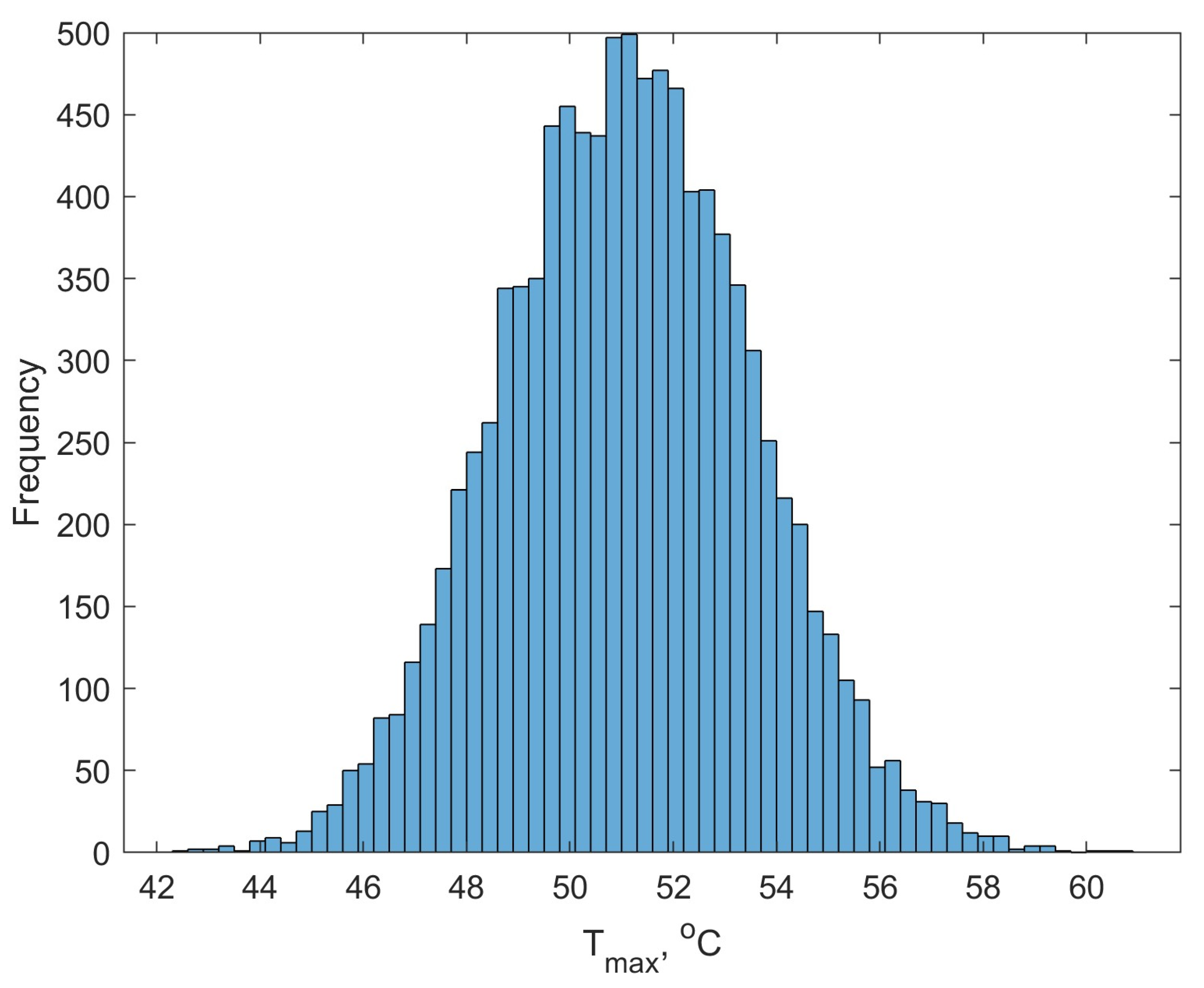
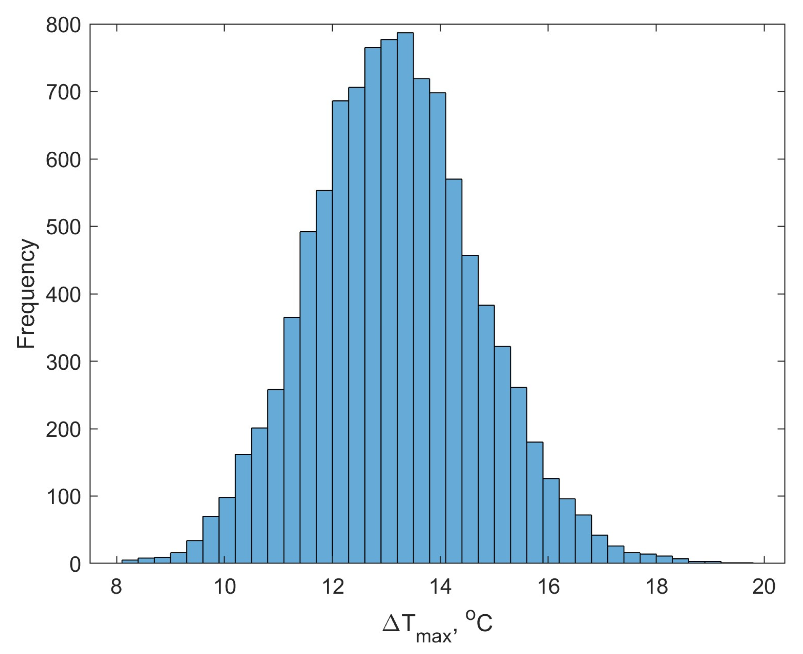
The proposed model also takes into account the variability of input parameters. To do this, it must be used in combination with the Monte Carlo method. For all input parameters except slab thickness and curing rate, n random values (n = 10,000) are generated, distributed normally with a given mathematical expectation and standard deviation. For n samples, T_max and ∆T_max are predicted using trained models, and histograms of the distribution of output parameters are constructed. It is also possible to estimate the probability of the predicted values exceeding the permissible limits as the ratio of the number of cases in which the output parameters exceeded the permissible limit to the total number of cases n.

Let us give an example of the calculation for a wall that was considered in [48]. The wall thickness in this experiment was 1 m, the average ambient temperature was 22 °C, the initial temperature of the concrete mixture was 25 °C, and the heat transfer coefficient was 9 W/(m²·°C). The concrete heat release value was 93 MJ/m³. The concrete hardening rate was slow-hardening. The formwork removal time was 7 days.

Table 8. Accepted standard deviations.

Parameter	T0, °C	T∞, °C	Q28, MJ/m3	α, W/(m2∙°C)
Standard deviation	2	2	5	1

shows the accepted standard deviations for the input parameters of the model that can vary (ambient temperature, initial concrete mix temperature, heat transfer coefficient and concrete heat release).

Figure 11 and Figure 12 show histograms of the distribution of the output parameters T_max and ∆T_max.

The average values of the output variables T_max and ∆T_max, based on the results of 10,000 simulations, are 51.1 °C and 13.2 °C, respectively. According to the results of the experiment, these values were T_max = 54 °C and ∆T_max = 12 °C. The probability of exceeding the permissible values T_max = 70 °C and ∆T_max = 25 °C for the example considered is zero.

The proposed approach, based on a combined use of the Monte Carlo method and CatBoost, allows for input data uncertainty to be taken into account. However, the CatBoost algorithm by default does not provide prediction uncertainty. To obtain prediction intervals for boosting, specialized methods are needed: quantile regression forests/quantile boosting, conformal prediction, ensemble bootstrapping, or Bayesian neural networks/Gaussian processes. This will be a promising area for further research.

5. Conclusions

Machine learning models based on the gradient boosting algorithm were developed and validated using a large dataset of 855,360 FEM simulations. CatBoost was used to predict the maximum temperature T_max and the maximum center-to-surface temperature difference ΔT_max in hardening massive monolithic walls. Unlike previous studies, the proposed approach takes into account variable heat transfer conditions at the surfaces, the concrete curing rate (rapid, normal, and slow), and the curing time of the structure in the formwork.

The models achieve R² > 0.99 and a MAPE of 0.2% for T_max and 3% for ΔT_max, demonstrating high forecast accuracy. An analysis of the feature importance revealed that the cement heat release Q₂₈ has the dominant influence on both target variables (42.9% for T_max and 35.3% for ∆T_max). The second most significant factor is the wall thickness H. The concrete curing rate significantly influences heating kinetics, while curing time in the formwork has a minimal contribution, consistent with the physics of the process.

A comparison of the developed model with the data of the independent study by [39] demonstrated good convergence: the average ratio of ∆T_max values was 0.97, and for T_max, it was 1.14. The systematic discrepancy in the maximum temperature (about 14%) is explained by differences in the modeling methods (solving the differential equation of thermal conductivity in the present work versus the simplified CIRIA C766 method in [39]).

The developed models allow engineers to assess temperature indicators of early cracking risk without FEM software. A trained CatBoost model runs at <0.1 s per case, enabling parametric studies (e.g., finding the maximum permissible heat release of concrete). For field use, we provide a Python script and an Excel workbook with examples of the input data (see the Data Availability Statement). The proposed model also allows one to take into account variations in input parameters when used in conjunction with the Monte Carlo method and to estimate the probability of exceeding the permissible limits for the maximum temperature and temperature difference. The model is valid within the parameter ranges used to generate the training dataset (ambient temperature: 5–30 °C, initial temperature of the concrete mix: 5–25 °C, wall thickness: 0.75–3 m, concrete heat release: Q₂₈ = 50–250 MJ/m³, and heat transfer coefficient: 1–23 W/(m²·°C)). Outside this range, extrapolation is not recommended.

Further research involves expanding the dataset by considering different heat transfer conditions on opposite wall surfaces and a wider range of climatic conditions (including subzero temperatures and extreme heat). The current model primarily reproduces the behavior of the numerical simulator, and broader experimental validation is required before widespread engineering applications.

It should be noted that the fully factorial and uniformly distributed dataset may not accurately represent realistic construction scenarios. In practice, many parameter combinations are rare, correlated, or physically improbable. Consequently, the model may be overly optimized for mathematically structured data rather than realistic engineering distributions. Future work can also consider probabilistic sampling approaches such as Latin Hypercube Sampling or real statistical distributions derived from construction practice to improve representativeness.

There is also another limitation of this study. The developed model predicts only temperature-related indicators (T_max and ΔT_max) rather than actual cracking behavior. While these quantities are strongly related to thermal cracking risk, crack formation also depends on tensile strength development, creep, shrinkage, and restraint conditions. Therefore, the model functions mainly as a surrogate thermal assessment tool rather than a direct cracking predictor. Further research could be aimed at developing machine learning models that directly predict stresses in a structure.