Interpretable Urban Building Energy Modeling by Heterogeneous Graph Neural Networks: A Case Study of Residential Blocks in Wuhan

Abstract

Traditional urban building energy modeling often overlooks the complexity of spatial configurations and mutual shading effects, thereby limiting its accuracy. This study proposes a novel, interpretable, data-driven framework based on heterogeneous graph neural networks (GNNs) to uncover and characterize the complex interrelationships between building morphology and urban topology. Using a parametric platform, this study generated a graph dataset of 285 residential blocks in Wuhan, structured as a dual-level graph: Building Zone Graphs (BZGs) and Building Layout Graphs (BLGs). Four GNN models were trained based on the dataset, and the evaluated results demonstrate that GraphTransformer outperforms GCN, GAT, and GraphSAGE in capturing long-range spatial relationships―particularly those arising from shading and solar access interactions. On a validation set, GraphTransformer achieved superior predictive accuracy, with R² scores exceeding 0.85 and 0.90 for cooling and heating energy predictions, respectively. After that, post hoc interpretability analysis by GNNExplainer identified three important morphology features influencing building energy consumption. Critically, the model found that shading relationships encoded as graph edges―especially those between southern and western façades―had statistically significant influence on building energy consumption. Finally, this work establishes an efficient, interpretable surrogate modeling framework for urban-scale energy analysis, delivering quantifiable, design-actionable insights to support sustainable urban development.

1. Introduction

Urban areas are dominant contributors to global energy consumption, accounting for over 60% of the total final energy use worldwide [1]. Driven by accelerating urbanization and sustained population growth, the demand for building energy is projected to increase [2]. It has been shown that the worldwide energy use may increase in 2050 by almost 90% with respect to the 2003 values [3]. Also, it has been predicted that the primary energy may rise by 70% from 2013 to 2050 [4]. Since most of the growing need is given by nonrenewable energy, this has led to some very important ecological consequences, such as global warming [5] and air pollution [6,7,8]. The international agreement has been already reached in need of a reduction of both the energy use and the carbon emission. In this context, precise urban building energy modeling (UBEM) [9,10] has become essential for evaluating energy efficiency potentials of buildings; developing urban design strategies; and supporting the shift to sustainable, low-carbon urban environments.

With the increase in academic research on urban energy consumption, techniques like building energy modeling (BEM) [11,12] and building performance simulation (BPS) [3,13] are widely used. The move from BEM to urban building energy modeling (UBEM) is a move from the analysis of a single building to the analysis of a complex urban environment [14]. The UBEM is an important planning tool for architects, city designers, and governments that make energy policies [15]. Traditionally, UBEM methods are divided into “top-down” and “bottom-up” approaches.

Top-down approaches treat the building volumes as a uniform unit, linking factors such as macroeconomic indicators [16] and climate conditions [17] to calculate energy consumption [18,19]. These models need limited data input; however, they do not account for the architecture details and the spatial relations (i.e., inter-building effects) of the compact urban building layout [20].

In contrast, bottom-up methods analyze energy consumption based on detailed end-use data, which are further classified into physics-based and data-driven models [21]. Physics-based models rely on thermodynamic laws and BPS [22], such as EnergyPlus [12] (platforms such as CityBES [23] or UMI [24]). Although capable of high-fidelity simulations, they demand extensive computational resources and input data, which are often unavailable at a city scale, leading to a reliance on default assumptions that compromise accuracy [3,5,25]. Data-driven models have emerged as a prominent alternative [26,27,28], using machine learning algorithms (e.g., support vector machines (SVMs) [29] and gradient boosting algorithms (XGBoost) [30]) and deep learning architectures (e.g., Recurrent Neural Network [31] and Artificial Neural Network [32]). However, the complex spatial characteristics of an urban layout and the impact of inter-building effect (IBE) often result in significant errors in the predictions of data-driven models. Additionally, since many data-driven models are black boxes [33,34], their interpretability is limited, which prevents their more general use in urban planning and policy making [5].

Graphs, as data structures that represent connected elements, provide an excellent way to describe urban layouts [35,36]. Graph structures are similar to network structures in that they can both describe the signal transmission and aggregation between nodes [37]. However, their irregular topology gives challenges for conventional neural networks (CNNs), which fail to capture the relationships from the dataset since CNNs require data arranged in grids or sequences [38]. To address this limitation, graph neural networks (GNNs) have emerged as a promising alternative by aggregating information from neighboring nodes. In the context of urban block design, GNN-based surrogate models offer the following advantages: they simultaneously account for individual building morphology and surrounding environment, exhibiting superior generalizability for different types of urban morphology [39]. The existing literature created a Shadow Attention Graph Neural Network (SAGNN) to advance solar radiation forecasting for urban edifices, thereby facilitating the realization of Net-Zero Energy Buildings (NZEBs) in New York City [40]. Concurrently, multi-building load prediction has been framed as a spatial contextual learning paradigm, wherein inter-building interactions are explicitly formalized by graph representations utilizing three years of hourly power consumption data across 24 facilities, integrated with coupled meteorological variables and EnergyPlus-simulated solar profiles [41]. These advancements emphasize the efficacy of GNNs in simulating building physics under urban microclimates, verifying that graphs can capture shading effects among adjacent buildings. Recent studies have constructed heterogeneous graphs encapsulated multidimensional urban entities―including buildings, streets, intersections, and plots [42]. Through relation-aware message passing and feature fusion, such frameworks successfully map intricate urban environments into structured topological data to predict localized building attributes.

Despite these advancements, current GNN-based UBEM research still has many important problems:

• Context limitation: BEM-focused GNN studies often use homogeneous graphs for internal zones and overlook external environmental influences from surrounding buildings [43].
• Morphological simplification: Existing UBEM studies often simplify buildings into single nodes, thereby failing to account for the impact of detailed building shape on energy performance [44].
• Algorithm limitation: Most studies only used one or two GNN algorithms, ignoring the significant differences in aggregation strategies among different GNN architectures and thereby limiting the robustness of the findings [45].
• Interpretability issues: There is an absence of post hoc interpretability analysis, which means that the underlying “decision-making” processes of these surrogate models remain unverified [46].

To address these gaps, this study introduces a novel, interpretable, data-driven UBEM framework designed to integrate IBE for accurate and widely applied urban building energy prediction. The block-level relationship graph (BRG) is a special heterogeneous graph [47] dataset which is constructed in a systematic way to record the building forms and urban spatial layout by parametric modeling methods. By evaluating and comparing four GNN architectures (Graph Convolutional Network (GCN), Graph Sample and Aggregation (GraphSAGE), Graph Attention Network (GAT), and GraphTransformer), this study identified the optimal model for urban building energy prediction. Finally, the GNNExplainer algorithm was used to perform an interpretability analysis, quantifying feature importance and visualizing signal-propagation patterns to verify the physical rationality of the predictive mechanism of the final model.

The objectives of this research are as follows:

• Heterogeneous graph datasets: This study develops 285 block-level relationship graphs for Wuhan City. Urban block information is converted into a multidimensional graph dataset that effectively captures building morphology and building topological layout features.
• GNN architectures comparison: This study evaluates and compares several GNN algorithms―including GCN [48], GraphSAGE, GAT, and GraphTransformer [49,50]―to identify the best architecture for predicting building energy consumption of the residential blocks in Wuhan.
• Model interpretability analysis: This study uses GNNExplainer [51,52] to open “the black box” of GNN surrogate models. The objective is to explain the internal decision-making processes and identify the key morphological indicators that influence block energy consumption.

2. Methodology

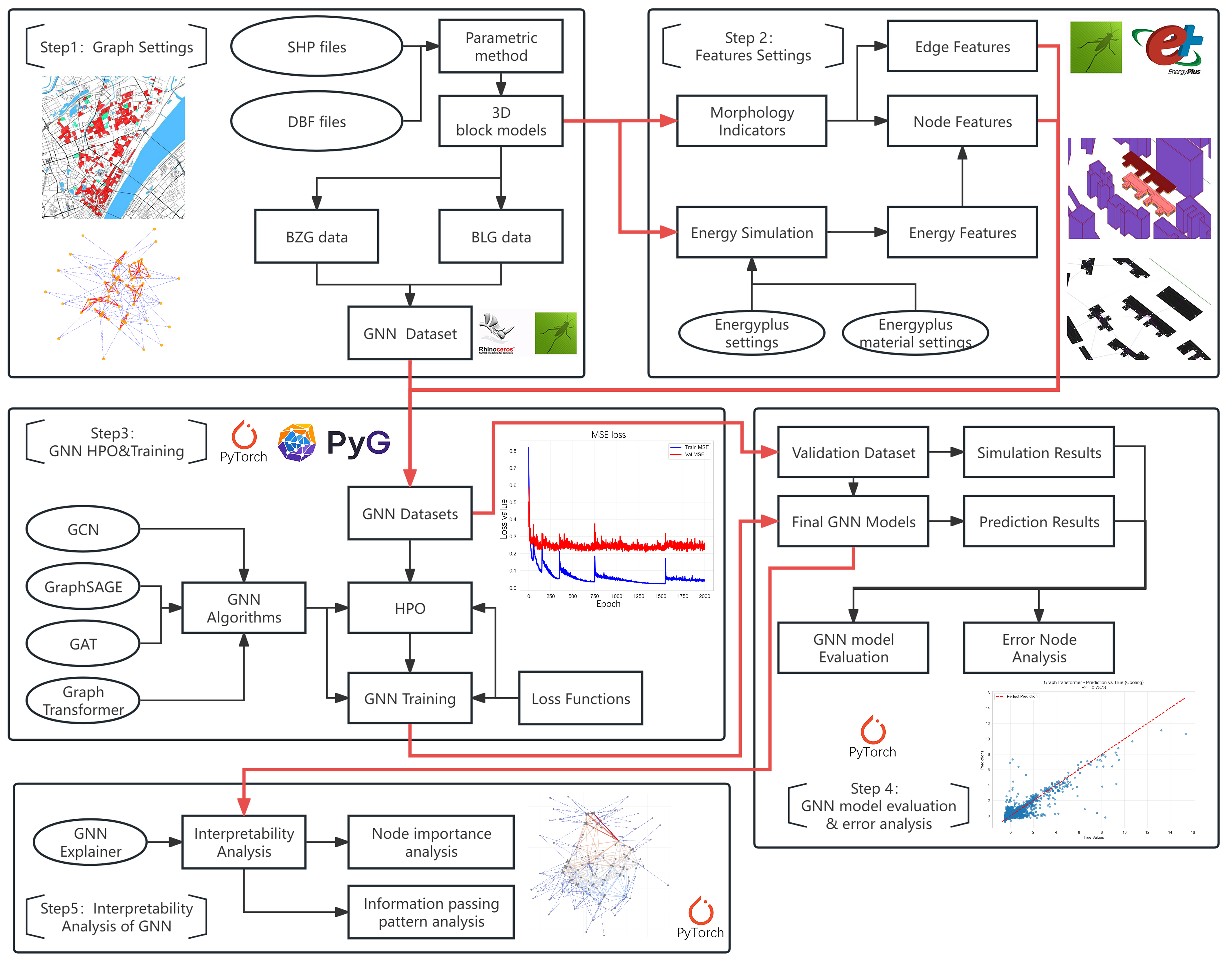
As shown in Figure 1, this section shows the research framework, which integrates graph data generation, building energy simulation (BES), GNN model training and validating settings, and GNNExplainer settings:

Figure 1. The workflow diagram of this study.

• Phase I (graph construction): Based on urban block building information, this study generates heterogeneous graph data by parametric methods (Section 2.1). The graph architecture comprises two connection types: (1) the Building Zone Graph (BZG) and (2) the Building Layout Graph (BLG).
• Phase II (feature engineering): Morphological indicators are used to define node and edge features in each graph. Concurrently, node-level energy consumption features are generated by the BPS method (Section 2.2).
• Phase III (algorithm architecture): Four GNN algorithms are introduced in Section 2.3. This phase also introduces the heterogeneous graph encoding strategies specific to each GNN algorithm.
• Phase IV (model training and optimization): The baseline and the search space of hyperparameter settings in four GNN algorithms are introduced. Subsequently, the models are trained and evaluated using a multi-objective loss function strategy (Section 2.4).
• Phase V (interpretability analysis): Post hoc interpretability of the GNN models is conducted using the GNNExplainer algorithm to identify key features and verify physical rationality (Section 2.5).

2.1. Graph Construction

The urban system exhibits a complex hierarchical structure, which stems from the interaction, feedback effect, and scaling process of urban form and function across multiple levels [53]. This study uses a heterogeneous graph method to effectively represent the detailed morphological features of individual buildings and their complex spatial relationships in urban blocks. Unlike traditional homogeneous graphs [54,55] that consist of only one type of node and edge, heterogeneous graphs include multilevel types of nodes and edges. By maintaining semantic information, the heterogeneous graph enables the investigation of deep connections between different types of nodes using techniques such as meta-paths.

This study proposes a dual-level graph framework, which hierarchically integrates the Building Zone Graph (BZG) and the Building Layout Graph (BLG). This hierarchical strategy enables a detailed representation of the morphological and topological features critical to energy performance analysis.

The dataset, comprising these heterogeneous graph sub-datasets, was divided as follows:

• Model training and testing (90%): This sub-dataset is used for training and validation, further subdivided into training (70%) and testing (30%) sets to support the iterative optimization of the four GNN algorithms.
• Final verification (10%): This part of the separate dataset is used as an independent validation set to verify predictive accuracy and generalizability of the final model when used for a different type of urban layout.

2.1.1. Heterogeneous Graph

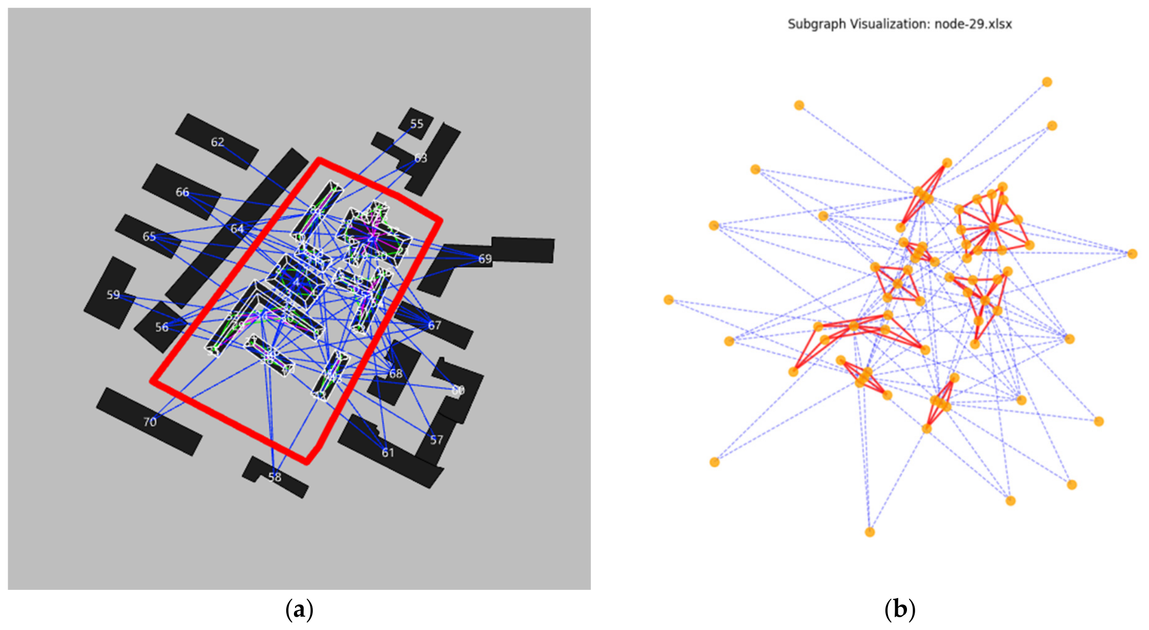
As illustrated in Figure 2a, the heterogeneous graph for each block is generated from the building layout by parametric modeling through a two-step process:

Figure 2. Residential building layout and heterogeneous graph visualization: (a) building layout; (b) double-layer heterogeneous graph structure.

• Building Zone Graph (BZG): Each building in the block is subdivided into functional zones. The topological connectivity between these zones is established to construct the BZG, which captures the internal spatial relationships of the building.
• Building Layout Graph (BLG): The centroids of buildings―both in the target block and in the surrounding context―are extracted. Connections are then established between these centroids to form the BLG, which represents the urban layout.

As shown in Figure 2b, the heterogeneous network integrates these two types of sub-graph: BZG edges (red) represent inter-zone connectivity, whereas BLG edges (blue) represent inter-building spatial relationships.

2.1.2. BZG Configuration

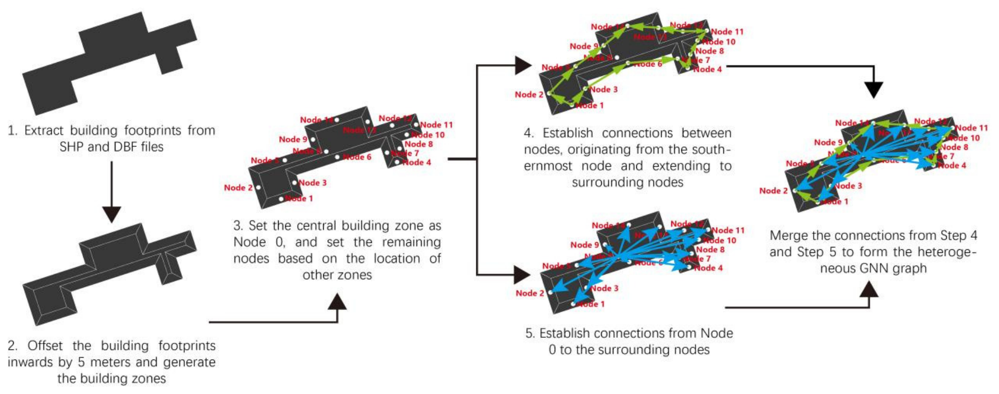
As shown in Figure 3, the generation process for the Building Zone Graph (BZG) is defined by the following two steps:

Figure 3. BZG generation process visualization.

• Node definition: Each building footprint was processed with a 5 m internal offset to create a central core zone (${Zone}_0$), representing the interior thermal space [43]. The remaining peripheral area was subsequently divided into $n$ directional zones (${Zone}_1$ to ${Zone}_n$) based on their spatial orientation.
• Edge definition:

  (1)

  Core-to-peripheral connectivity: Directed edges are established from the centroid of the core node (${Zone}_0$) to each centroid of the $n$ nodes (${Zone}_1$ to ${Zone}_n$).

  (2)

  Peripheral-to-peripheral connectivity: Directed edges are established between the adjacent peripheral zones. To maintain directional consistency and minimize topological redundancy, these edges originate from the centroid of the south-facing zone and extend sequentially to its neighboring zones.

2.1.3. BLG Configuration

As shown in Figure 2a,b, to address the significant variability in building layouts of the residential blocks in Wuhan, a standardized and simplified graph model is created by a three-step process:

• Node definition: Each building in the target block is represented by a node set at the centroid of its core zone (${Zone}_0$). Because neighboring buildings outside the block may influence the microclimate in the target block, surrounding buildings within a 200-meter radius around the block are included in the graph. These surrounding buildings are represented by single nodes at their geometric centers.
• Edge generation: Connections between nodes are established based on layout. Initially, all possible pairwise links between buildings inside the block and the neighboring external buildings are generated.
• Edge filtering: To optimize GNN efficiency, edge filtering thresholds were determined based on the physical and solar boundary conditions of Wuhan. (1) $F_{distance}$ (200 m): the residential buildings in Wuhan are generally under 100 m (33 stories). The 200 m threshold represents twice the maximum building height, ensuring all critical mutual shading is captured. (2) $F_{angle}$ ($-45°$ to $45°$): Wuhan is located at $30.5° \mathrm{N}$ latitude. Based on solar azimuth trajectories in the Northern Hemisphere, context buildings located in the due-north sector of a target building ($-45°$ to $45°$) will never cast solar shadows onto the target building. The $F_{distance}$ and $F_{angle}$ are detailed in Table 1.
  Table 1. Edge filtering method.

  Nomenclature	Range	Description
  $F_{angle}$	$-45° \le F_{angle} \le 45°$	$F_{angle}$ is the angle between the edge connecting the target node to a surrounding building node and the north–south axis; edges corresponding to $F_{angle}$ values within the specified range are eliminated.
  $F_{distance}$	$F_{distance}\ge 200 \mathrm{m}$	$F_{distance}$ is the edge distance between the target node and the surrounding building node; edges for which $F_{distance}$ exceeds the threshold are eliminated.

2.2. Feature Engineering

This study used parametric methods to extract a set of features for both nodes and edges. For node features, morphological indicators of the corresponding building zones are generated to serve as node morphology features. Simultaneously, building energy consumption for each zone in the block is simulated with EnergyPlus, and the simulation results are integrated as node energy features. Additionally, edge features are also generated using the same parametric framework to complete the dataset for the GNN models.

2.2.1. Node Morphology Features

Previous studies have shown that differences in building geometry significantly influence energy consumption. To capture the impact of these geometric characteristics, specific morphological indicators are incorporated into the GNN model as node features. Based on the previous research [23,56,57], this study identifies key indicators affecting building energy performance. Furthermore, although the graph topology captures the building layouts and relative connectivity, it does not explicitly represent the exact spatial coordinates of each zone. To address this limitation, two additional indicators are introduced to define the precise spatial relationship between each node and the center of the block. Using the block center as the origin, the east–west distance (${\mathrm{D}}_{\mathrm{x}}$) and north–south distance (${\mathrm{D}}_{\mathrm{y}}$) were calculated for each node. ${\mathrm{D}}_{\mathrm{x}}$ and ${\mathrm{D}}_{\mathrm{y}}$ were integrated into the GNN model as supplementary morphological features, as detailed in Table 2.

Table 2. Node morphology feature settings.

Nomenclature	Description	Unit
$Area$	The floor area of the building zone	${\mathrm{m}}^2$
$BH$	The height of the building block corresponds to the building zone	$\mathrm{m}$
$L/W$	The length-to-width ratio of the building zone	none
$OZ$	The angle between the outward normal of the zone exterior wall and true north.	°
$D_x$	The distance between node and the center of the block on the east–west axis	$\mathrm{m}$
$D_y$	The distance between node and the center of the block on the south–north axis	$\mathrm{m}$

2.2.2. Node Energy Features

This study uses Energy Use Intensity (EUI) [58] as the main indicator for evaluating building energy performance. Since Wuhan is a typical hot-summer and cold-winter city, both the summer-cooling and winter-heating energy load of buildings are critical considerations [59]. Accordingly, EUI is defined as the annual building average heating (${\mathrm{F}}_{\mathrm{H}\mathrm{e}\mathrm{a}\mathrm{t}\mathrm{i}\mathrm{n}\mathrm{g}}$) and cooling (${\mathrm{F}}_{\mathrm{C}\mathrm{o}\mathrm{o}\mathrm{l}\mathrm{i}\mathrm{n}\mathrm{g}}$) system loads for all vertical spaces within each building zone, providing a comprehensive representation of the annual energy demand. The node energy features are summarized in Table 3.

Table 3. Node energy feature settings.

Nomenclature	Description	Unit
$F_{Heating}$	Winter heating-system energy consumption of the building zone	$\mathrm{k}\mathrm{w}·\mathrm{h}$
$F_{Cooling}$	Summer cooling-system energy consumption of the building zone	$\mathrm{k}\mathrm{w}·\mathrm{h}$

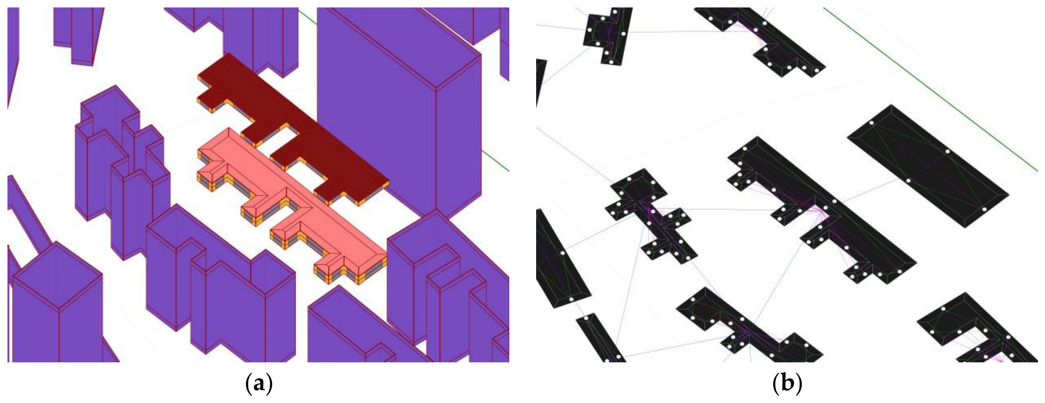
To reduce the high computational costs associated with large-scale, block-level energy simulations, a three-layer simulation strategy [60]―comprising bottom, middle, and top building floors―is used, as shown in Figure 4a. In Figure 4b, each node in the graph represents the aggregated energy consumption of all vertical building units within its corresponding zone. This abstraction enables efficient modeling while maintaining high simulation accuracy.

Figure 4. (a) Building simulation settings; (b) building node settings.

The building annual heating (${\mathrm{F}}_{\mathrm{H}\mathrm{e}\mathrm{a}\mathrm{t}\mathrm{i}\mathrm{n}\mathrm{g}}$) and cooling (${\mathrm{F}}_{\mathrm{C}\mathrm{o}\mathrm{o}\mathrm{l}\mathrm{i}\mathrm{n}\mathrm{g}}$) loads were simulated by EnergyPlus [61] with Typical Meteorological Year (TMY) data [62]. The simulations were performed within the Grasshopper parametric platform, using the Honeybee [63,64] and Dragonfly [58,65] plugins. To align with the template-based workflow of Dragonfly, the initial configurations were based on the ASHRAE 90.1-2015 standard [66].

Furthermore, to reflect local conditions in Wuhan, the simulation parameters were adjusted to follow with regional design codes. Consequently, key parameters, including building envelope materials, internal heat gains, lighting power densities, occupant densities, HVAC set points, and operational schedules, were set according to both national (GB50189-2015) and regional (DB42/301-2023) standards. These simulated results were then normalized and integrated with the previously established graph structures and node features to create the database for training and validating the GNN models. The detailed simulation settings and material properties are summarized in Table 4, Table 5 and Table 6.

Table 4. Initial simulation settings.

Simulation Setting	Setting	Description
Climate zone	4 Mixed ASHRAE climate zone	Wuhan location (Typical hot-summer and cold-winter climate)
Building vintage	ASHRAE 90.1 2015	Structures built between 2014 and 2018
Function	Mid-rise apartment	Typical Wuhan residential building
Structure	Mass	Mid-rise residential building construction type

Table 5. Details of simulation settings.

Simulation Setting	Value	Unit	The Setting Name	Value	Unit
Number of people per area	0.1	per/m2	Ventilation per person	0.008	m3/s per person
Equipment loads per area	15.00	W/m2	Recirculated air per area	0	m3/s per m2
Lighting density per area	9.00	W/m2	Lighting power	250	W
Infiltration rate per area	0.0003	m3/s per m2	Lighting set point	300	Lux
Ventilation per area	0.001	m3/s per m2

Table 6. Material details of settings.

Construction Name	Material Name	Roughness	Thickness (m)	Conductivity (W/m-K)	Density (kg/m3)	Specific Heat (J/kg-K)	Thermal Absorptance	Solar Absorptance	Visible Absorptance
Wall	Cement-based insulation mortar	Medium Rough	0.10	0.049	265	836.8	0.9	0.7	0.7
	Brick	Medium Rough	0.20	0.810	1920	790	0.9	0.7	0.7
Roof	Cement-based insulation mortar	Medium Rough	0.10	0.049	265	836.8	0.9	0.7	0.7
	Concrete	Medium Rough	0.20	1.7496	2243	837	0.9	0.7	0.7
Floors	Concrete	Medium Rough	0.15	0.53	1280	840	0.9	0.5	0.7
Construction name		Material name		U-value (W/m2·K-1)		SHGC		VT
Window glass		Low-E glass		2.50		0.60		0.50

2.2.3. Edge Features

Although heterogeneous graphs effectively capture the relationships between building nodes both within and surrounding the block, these edges typically represent topological connections. To ensure the model accounts for real-world geometric information, it is essential to specify physical attributes such as distance and orientation. This study defines edges using two features: edge angle (${\mathrm{E}}_{\mathrm{a}\mathrm{n}\mathrm{g}\mathrm{l}\mathrm{e}}$) and edge distance (${\mathrm{E}}_{\mathrm{d}\mathrm{i}\mathrm{s}\mathrm{t}\mathrm{a}\mathrm{n}\mathrm{c}\mathrm{e}}$). The edge features are summarized in Table 7.

Table 7. The edge features’ settings.

Nomenclature	Description	Unit
$E_{angle}$	$E_{angle}$ is the angle between the edge connecting the nodes and the north–south axis.	°
$E_{distance}$	$E_{distance}$ is the edge distance between the two nodes.	m

Because some GNN architectures, such as GCN and GraphSAGE, are not designed to process multidimensional edge features directly, a mapping transformation method is used. This method converts the multidimensional edge attributes into optimized scalar weights to ensure compatibility with the message-passing mechanisms of all GNN models.

2.3. GNN Algorithms

Different GNN algorithms use different information aggregation mechanisms, leading to variations in how they handle multilevel edge relationships and features. These methodological differences often result in performance differences when models are trained on complex heterogeneous graphs. To comprehensively evaluate the performance of GNNs on the two-hop heterogeneous graphs, this study uses four GNN architectures with different aggregation approaches, as summarized in Table 8. These four GNN algorithms exhibit algorithmic divergence in their information aggregation paradigms and network. To systematically evaluate the efficacy of attention mechanisms, performance benchmarks were established comparing two non-attentional frameworks (GCN and GraphSAGE) against two attention-driven GNN algorithms (GAT and GraphTransformer). Furthermore, a comparative analysis between GAT and GraphTransformer was used to discern the operational effectiveness and representational capacities of localized versus global attention mechanisms within the building energy prediction.

Table 8. The mechanism and aggregation method of four GNN algorithms.

GNN	Mechanism	Aggregation Method
GCN	Spectral graph convolution approximation	Fixed-weight averaging
GraphSAGE	Neighborhood sampling and aggregation	Aggregation by learnable functions
GAT	Graph Attention	Dynamic calculation of attention weights based on features
GraphTransformer	Global self-attention	Global node interaction integrated with structural information

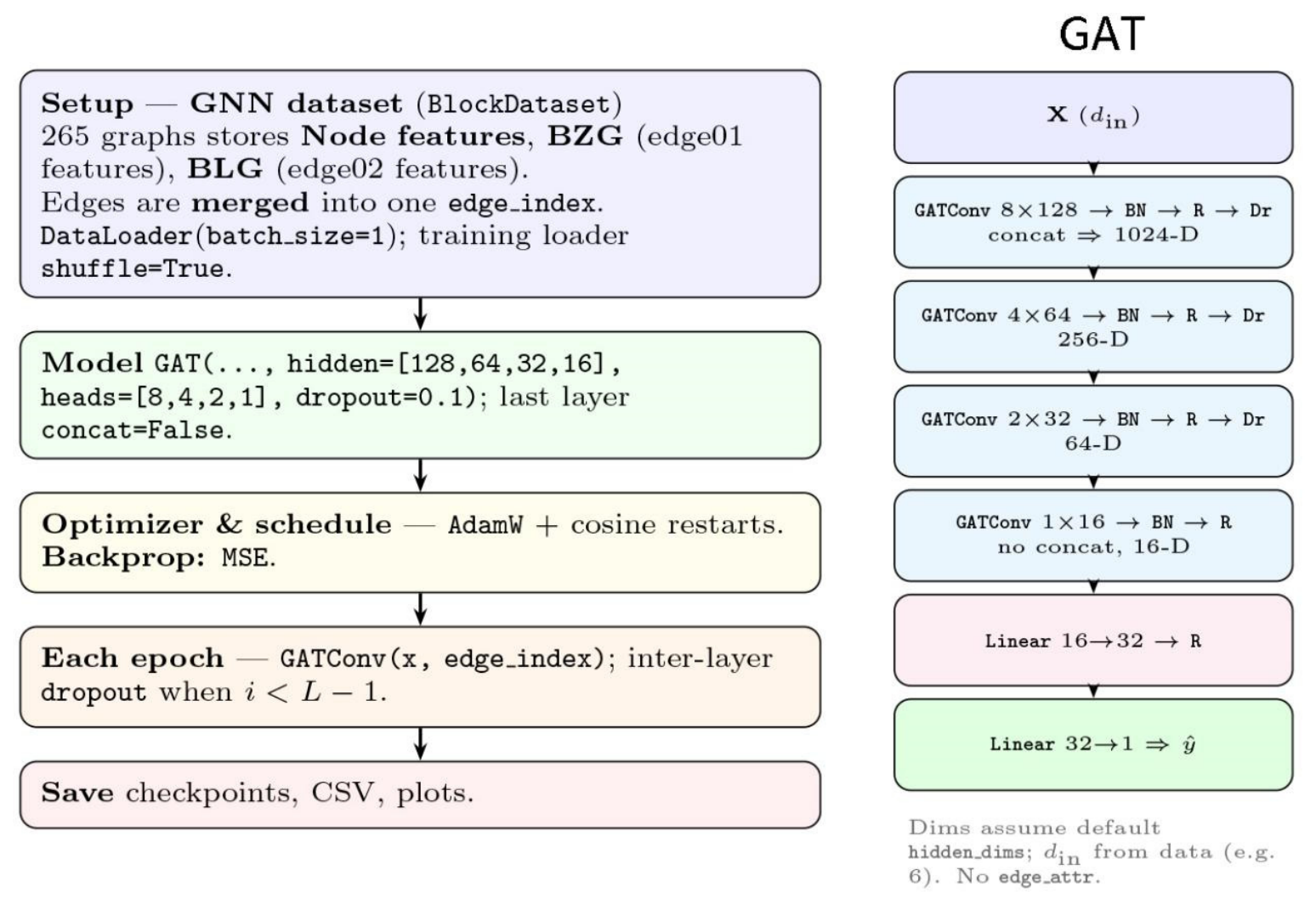
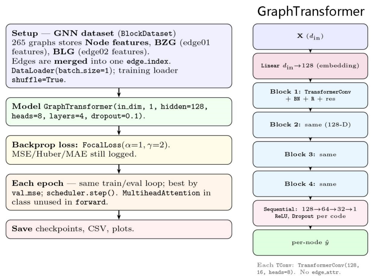
To ensure a rigorous and consistent comparison, all relationship types are classified into one-hop edges (edge 1: BZG) and two-hop edges (edge 2: BLG). In the encoding phase, all four models use a unified framework characterized by relation-specific message passing, fusion through cross-relation summation, and nonlinear transformations between layers. This standardized pipeline ensures fairness between all models.

The main difference between the GNN models is how they handle message passing and incorporate features:

• GCN and GraphSAGE: These models convert edge features into scalar weights before performing weighted propagation. This approach aligns with spectral-domain normalized aggregation for GCN, and neighborhood means aggregation for GraphSAGE.
• GAT and GraphTransformer: These architectures directly integrate edge features into attention-based calculations. They utilize multi-head mechanisms to learn the relative contributions of different neighboring edges, including two-hop connections, to the target node.

2.3.1. Graph Convolutional Network (GCN)

GCN is a spectral-based GNN that is designed for graph-structured data. Its core mechanism relies on message passing and neighborhood aggregation, in which nodes are updated through a weighted combination of features from adjacent nodes. The layer-wise propagation rule is defined as follows:

$$H^{ (l + 1)} = \sigma ({\tilde{D}}^{-{\displaystyle \frac{1}{2}}}\tilde{A}{\tilde{D}}^{-{\displaystyle \frac{1}{2}}}{H}^{\left(l\right)}{W}^{\left(l\right)})$$

(1)

where $\tilde{\mathrm{A}}=\mathrm{A}+\mathrm{I}$ is the adjacency matrix with added self-loops, $\mathrm{D}$ is the corresponding diagonal degree matrix, ${\mathrm{H}}^{\left(\mathrm{l}\right)}$ represents the node feature matrix at layer $\mathrm{l}$, ${\mathrm{W}}^{\left(\mathrm{l}\right)}$ is a learnable weight matrix, and $\mathrm{\sigma }(\cdot )$ denotes the nonlinear activation function.

GCN supports transductive learning, enabling effective representation learning for graph structures. Furthermore, by sharing parameters among nodes, they greatly decrease the complexity of the model and the computational cost. However, the GCN architecture is susceptible to over-smoothing, in which multiple rounds of aggregation cause node embedding to become too similar, reducing their ability to distinguish between nodes. Additionally, GCN typically assumes a fixed graph topology, making it less adaptable to dynamic variations in node or edge features than inductive models.

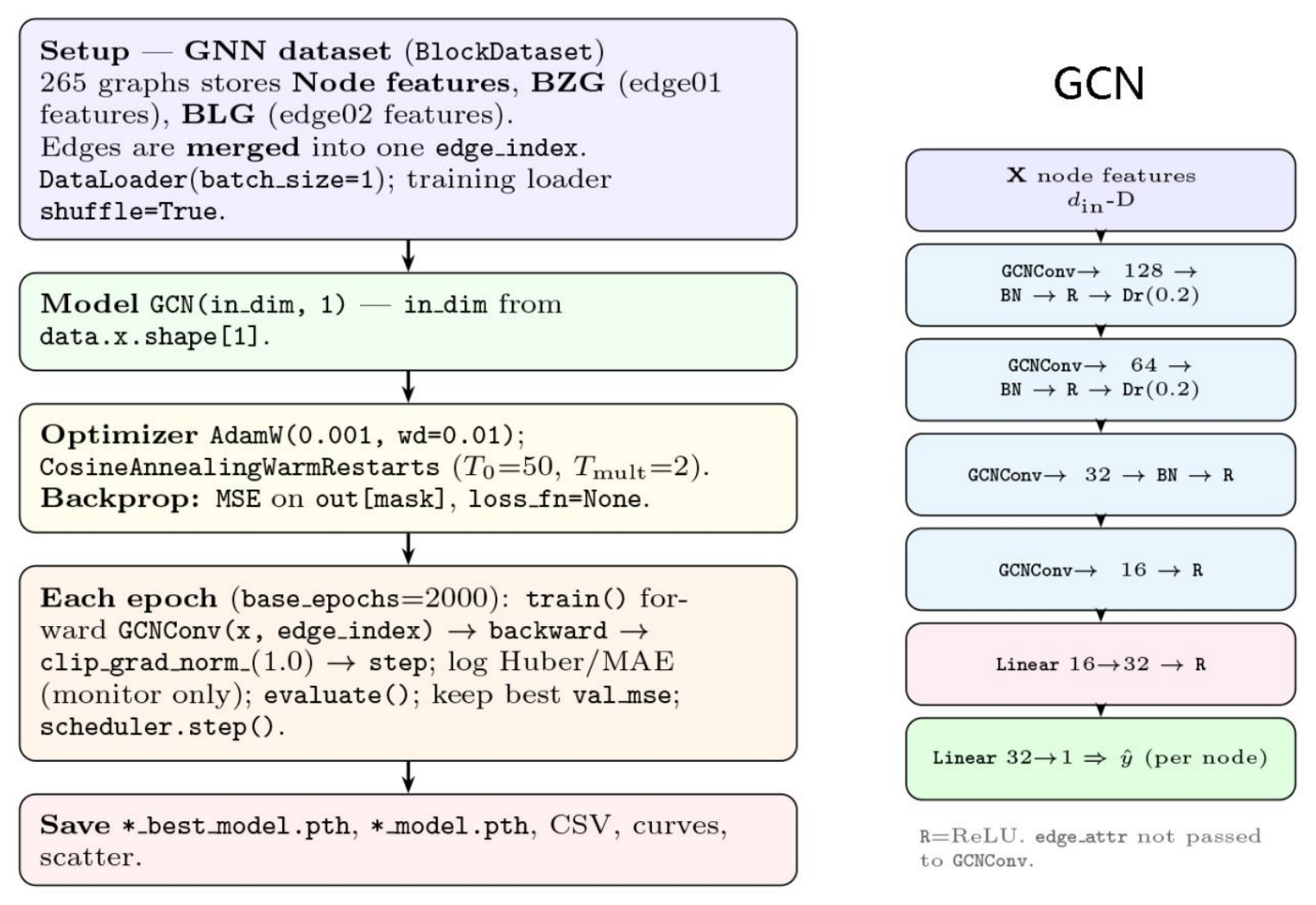
As shown in Figure 5, when processing two-hop heterogeneous graph data, the GCN uses a framework of “relation-specific decomposition, per-relation convolution, and summation aggregation”. Message passing is performed independently for edge 1 and edge 2, with the results from each relationship subsequently aggregated by summation. To balance the information propagation weights between BZG and BLG in the GNN model, the edge weights for Edge 1 and Edge 2 were set equally at 0.5. This explicit weighting configuration ensures that the predictive model concurrently encapsulates both inter-building spatial layouts and room-to-room topological relations during energy prediction.

Figure 5. The workflow diagram of GCN.

For integrating edge features, the GCN maps the multidimensional features (${\mathrm{E}}_{\mathrm{a}\mathrm{n}\mathrm{g}\mathrm{l}\mathrm{e}}$ and ${\mathrm{E}}_{\mathrm{d}\mathrm{i}\mathrm{s}\mathrm{t}\mathrm{a}\mathrm{n}\mathrm{c}\mathrm{e}}$) of all edges into scalar weights, which are then incorporated into the propagation process.

2.3.2. GraphSAGE

GraphSAGE is an inductive GNN framework that generates node embeddings by sampling and aggregating features from the local neighborhood of a node. Unlike transductive models, it supports inductive learning, which allows effective generalization to previously new nodes or completely new graph that were not seen. Different aggregation methods, including mean, LSTM, and pooling, can be used to integrate information from neighboring nodes. The core formulation of GraphSAGE is defined as follows:

$$h_u^{\left(k\right)} = \sigma (w^{\left(k\right)} \times {AGGREGATE}^{\left(k\right)}(\left\{h_v^{(k - 1)}, {\forall }_v\in N(u)\right\}))$$

(2)

In this equation, ${\mathrm{h}}_{\mathrm{v}}^{(\mathrm{k}-1)}$ is the feature vector of neighbor $\mathrm{v}$ from the neighborhood set, $\mathcal{N}\left(\mathrm{u}\right)$, at the preceding layer, ($\mathrm{k}-1$). ${\mathrm{A}\mathrm{G}\mathrm{G}\mathrm{R}\mathrm{E}\mathrm{G}\mathrm{A}\mathrm{T}\mathrm{E}}^{\left(\mathrm{k}\right)}$ is the function employed to fuse neighborhood features into a unified vector. ${\mathrm{W}}^{\left(\mathrm{k}\right)}$ represents the learnable weight matrix, while $\mathrm{\sigma }$ is the nonlinear activation function, enabling the model to capture complex, nonlinear patterns.

GraphSAGE follows an inductive learning approach, meaning the model learns a generalized aggregator function rather than fixed embeddings for each node. However, its random sampling process introduces variability during training, which may affect the stability of convergence. Furthermore, aggregating over a sampled subset of neighbors can result in information loss, particularly when critical structural details are missing during the sampling phase.

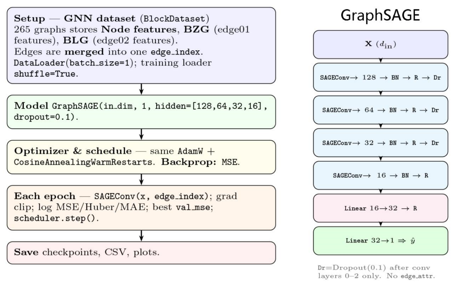
As shown in Figure 6, GraphSAGE processes two-hop heterogeneous graph data using a framework like GCN, characterized by “relation-specific decomposition, per-relation convolution, and summation aggregation”. For integrating edge features, GraphSAGE similarly maps all edge features into scalar weights (the scalar weight of edge 1 and edge 2 are both 0.5), which are then incorporated into the message propagation process to modulate the influence of different neighboring types.

Figure 6. The workflow diagram of GraphSAGE.

2.3.3. Graph Attention Network (GAT)

GAT improves the GCN framework by introducing a learnable attention mechanism that assigns adaptive weights to neighboring nodes, removing the need for predefined normalization based on node degrees. Rather than changing the fundamental “neighborhood aggregation” approach, GAT replaces fixed normalization with a learnable attention module. This advancement enables the model to adaptively assign importance to different neighbors based on the semantic content of their features.

To highlight this distinction, the aggregation method of GCN can be expressed as follows:

$$h_i = \sigma (\sum _{j\in N_i}\underset{fixed weight}{\underbrace{{\displaystyle \frac{1}{\widehat{d_i}\widehat{d_j}}}}}W{h}_j)$$

(3)

In contrast, the aggregation method for GAT is defined as follows:

$$h_i = \sigma (\sum _{j\in N_i}\underset{learnable weight}{\underbrace{a_{ij}}}W{h}_j)$$

(4)

In this mechanism, ${\mathrm{\alpha }}_{\mathrm{i}\mathrm{j}}$ represents attention weight. For a target node, $\mathrm{i}$, and its neighbor, $\mathrm{j}$, GAT first computes an attention score, ${\mathrm{e}}_{\mathrm{i}\mathrm{j}}$. Subsequently, a Softmax function is applied across the entire neighborhood, ${\mathcal{N}}_{\mathrm{i}}$, to normalize these scores, getting the final weights. The equations for ${\mathrm{e}}_{\mathrm{i}\mathrm{j}}$ and ${\mathrm{\alpha }}_{\mathrm{i}\mathrm{j}}$ are as follows:

$$e_{ij} = LeakyReLU\left(a^T\right[{Wh}_i\hspace{0.17em}\Vert \hspace{0.17em}{Wh}_j\left]\right)$$

(5)

$$a_{ij}={softmax}_j(e_{ij})= {\displaystyle \frac{exp\left(e_{ij}\right)}{\sum _{k\in N_i}epx\left(e_{ik}\right)}}$$

(6)

where LeakyReLU is the nonlinear activation function, $a$ is a learnable attention weight vector used to evaluate the importance of concatenated features, and $W$ is a learnable weight matrix for the linear transformation of node features. The ability of GAT to dynamically learn neighbor importance makes it particularly suitable for heterogeneous graphs with diverse node roles. Furthermore, attention weights provide inherent interpretability, enabling the visualization of influential spatial relationships. However, GAT is sensitive to noisy or spurious connections, which may distort the attention distributions.

As shown in Figure 7, when processing two-hop heterogeneous data, GAT utilizes a multi-head attention mechanism that inputs the two edge attributes into the model by independent relationship channels. These attributes directly influence the attention weights (the attention weight of edge 1 and edge 2 are both 0.5), allowing for a more refined integration of structural and geometric information.

Figure 7. The workflow diagram of GAT.

2.3.4. GraphTransformer

In the GraphTransformer architecture, given an input graph with node features ${\mathrm{X}}_{\mathrm{i}}\in {\mathbb{R}}^{{\mathrm{d}}_{\mathrm{i}\mathrm{n}}}$, each node is first projected into a shared hidden space via a linear embedding layer:

$$h_i^{\left(0\right)} = W_{emb}{X}_i + B_{emb},\hspace{1em}{W}_{emb}\in {\mathbb{R}}^{d_{hid} \times d_{in}}$$

(7)

The model stacks $L$ Transformer-based convolutional layers. At the $\mathrm{l}$-th layer, for each attention head, $\mathrm{k}$, the node representation, ${\mathrm{h}}_{\mathrm{i}}^{(\mathrm{l}-1)}$, is linearly projected into query (${\mathrm{q}}_{\mathrm{i}}^{\left(\mathrm{k}\right)}$), key (${\mathrm{k}}_{\mathrm{j}}^{\left(\mathrm{k}\right)}$), and value (${\mathrm{v}}_{\mathrm{j}}^{\left(\mathrm{k}\right)}$) vectors:

$$q_i^{\left(k\right)} = W_Q^{\left(k\right)}{h}_i^{(l - 1)}$$

(8)

$$k_j^{\left(k\right)}=W_K^{\left(k\right)}{h}_j^{(l-1)}$$

(9)

$$v_j^{\left(k\right)}={ W}_V^{\left(k\right)}{h}_j^{(l-1)}$$

(10)

The attention coefficient for an edge ($\mathrm{j}\to \mathrm{i}$) is computed as a scaled dot-product followed by a Softmax normalization over the neighborhood, $\mathcal{N}\left(\mathrm{i}\right)$:

$$e_{ij}^{\left(k\right)} = {\displaystyle \frac{(q_i^{\left(k\right)}{)}^T{k}_j^{\left(k\right)}}{\sqrt{d_h}}}$$

(11)

$$a_{ij}^{\left(k\right)}={\displaystyle \frac{\mathit{exp}(e_{ij}^{\left(k\right)})}{\sum _{t\in \mathcal{N}\left(i\right)}\mathit{exp}(e_{it}^{\left(k\right)})}}$$

(12)

The aggregated message for head $\mathrm{k}$ is then derived as follows:

$$m_i^{\left(k\right)} = \sum _{j\in \mathcal{N}\left(i\right)}{a}_{ij}^{\left(k\right)}{v}_j^{\left(k\right)}$$

(13)

The multi-head output is obtained by concatenating ${\mathrm{m}}_{\mathrm{i}}^{\left(\mathrm{k}\right)}$ across all heads. Each layer further incorporates Batch Normalization (BN) and a residual connection, followed by a ReLU nonlinearity:

$$h_i^{\left(l\right)} = \sigma (BN\left(m_i\right) + h_i^{(l - 1)})$$

(14)

where $\mathrm{\sigma }(\cdot )$ denotes the ReLU activation function. After $L$ layers, the final node embeddings, ${\mathrm{h}}_{\mathrm{i}}^{\left(\mathrm{L}\right)}$, are passed through a lightweight feed-forward network (FFN) to produce the scalar regression output, ${\widehat{\mathrm{y}}}_{\mathrm{i}}$, for each node.

As shown in Figure 8, GraphTransformer follows the established framework for processing two-hop heterogeneous graph data. Regarding edge feature integration, similar to GAT, GraphTransformer uses a multi-head attention mechanism to input the two edge features through independent relationship channels, where these features directly influence the calculation of attention weights to capture complex spatial relationships. The attention weights for Edge 1 and Edge 2 are uniformly set as 0.5 to sustain a relatively balanced information propagation paradigm between the BZG and BLG domains, thereby ensuring equalized feature contributions to the final GNN prediction outcomes.

Figure 8. The workflow diagram of GraphTransformer.

2.4. GNN Model Train and Evaluation

Model training and analysis were executed in a Python 3.12 environment using a computer comprised of an AMD Ryzen 9 7950X 16-core CPU, an NVIDIA GeForce RTX 4070 Ti GPU, and 64 GB of RAM. Before model training, hyperparameter optimization studies were conducted on the same computer to guarantee optimal configuration and architectural convergence for each GNN model.

2.4.1. Hyperparameter Optimization

Table 9 summarizes the baseline hyperparameter settings of the four GNN architectures. To improve the model performance, automated hyperparameter optimization (HPO) was conducted for each algorithm using the Optuna framework [67]. The HPO process aimed to minimize the MSE loss as the objective function, while maintaining the train/validation split consistently to ensure fair comparison among the models.

Table 9. Hyperparameter baseline settings.

Hyperparameter	GCN	GAT	GraphSAGE	GraphTransformer
Epochs for every trial	200	200	200	200
Optuna trials	30	30	30	30
Batch size	1	1	1	1
Learning rate	1 × 10−3	1 × 10−3	1 × 10−3	1 × 10−3
Weight decay	1 × 10−5	1 × 10−5	1 × 10−5	1 × 10−5
dropout	0.2	0.2	0.2	0.2
Train loss	MSE	MSE	MSE	MSE

For each GNN architecture, Optuna executed 30 independent trials. In every trial, the model was trained for 200 epochs (in total, 6000 training epochs for HPO), and the trajectory of the MSE loss on the validation set was monitored. The minimum MSE loss achieved within each trial was then returned as the objective value for optimization.

The specified search space (Table 10) includes key hyperparameters, such as optimizer settings (learning rate and weight decay), network size (number of layers, hidden units), and regularization methods (dropout). For attention-based architectures (GAT and GraphTransformer), the number of attention heads was also integrated into the search space. After the HPO process was completed, the best hyperparameter settings were selected to perform the final training of the surrogate models.

Table 10. Hyperparameter search space.

Hyperparameter	Range	Scale	Model
Learning rate	(1 × 10−4, 1 × 10−2)	log	ALL
Weight decay	(1 × 10−5, 1 × 10−1)	log	ALL
Dropout	(0.0, 0.4)	Linear	ALL
Hidden layer 1	{64, 128, 256}	categorical	GCN GraphSAGE GAT
Hidden layer 2	{32, 64, 128}	categorical	GCN GraphSAGE GAT
Hidden layer 3	{16, 32, 64}	categorical	GCN GraphSAGE GAT
Hidden layer 4	{8, 16, 32}	categorical	GCN GraphSAGE GAT
Hidden layer	{64, 128, 256}	categorical	GraphTransformer
Layer number	(2, 6)	integer	GraphTransformer
GAT heads	{2, 8}	categorical	GAT
GraphTransformer heads	{2, 8}	categorical	GraphTransformer

2.4.2. GNN Training and Evaluation

The training process was executed in mini batches, with model weights updated based on gradients calculated at each step. To ensure robustness and convergence, a multi-objective loss strategy was used in this study. The main loss function for back-propagation was Mean Squared Error Loss ($Los{s}_{MSE}$), which aimed to maintain overall predictive accuracy. At the same time, Huber loss ($\mathrm{L}\mathrm{o}\mathrm{s}{\mathrm{s}}_{\mathrm{H}\mathrm{u}\mathrm{b}\mathrm{e}\mathrm{r}}$) and Mean Absolute Error Loss ($\mathrm{L}\mathrm{o}\mathrm{s}{\mathrm{s}}_{\mathrm{M}\mathrm{A}\mathrm{E}}$) were tracked. $\mathrm{L}\mathrm{o}\mathrm{s}{\mathrm{s}}_{\mathrm{H}\mathrm{u}\mathrm{b}\mathrm{e}\mathrm{r}}$ enhances the model’s resilience to outliers, while $\mathrm{L}\mathrm{o}\mathrm{s}{\mathrm{s}}_{\mathrm{M}\mathrm{A}\mathrm{E}}$ provides a metric for error interpretation. The optimal model was identified at the bottom of the loss curve on the validation dataset.

For each node, $i$, in the GNN, the model generates a prediction, $\widehat{y_i}$, where $y_i$ represents the simulated ground truth. The equations for $Los{s}_{MSE}$ and $Los{s}_{MAE}$ are as follows:

$${Loss}_{MSE} = {\displaystyle \frac{1}{N}}{\displaystyle \sum _{i = 1}^N}{({\widehat{y}}_i -y_i)}^2$$

(15)

$${Loss}_{MAE}={\displaystyle \frac{1}{N}}{\displaystyle \sum _{i=1}^N}\left|{\widehat{y}}_i-y_i\right|$$

(16)

In terms of $Los{s}_{Huber}$, let $r_i$ denote the residual for each sample, defined as $r_i = y_i - {\widehat{y}}_i$. With the threshold, $\delta$, set to 1, $Los{s}_{Huber}$ is defined as follows:

$${\mathrm{l}}_{\mathrm{\delta }}({\mathrm{r}}_{\mathrm{i}})= \left\{\begin{array}{c}{\displaystyle \frac{1}{2}}{r}_i^2 \left|r_i\right| \le \delta \\ \delta (\left|r_i\right| - {\displaystyle \frac{1}{2}}\delta ) \left|r_i\right| > \delta \end{array}\right.$$

(17)

$${Loss}_{Huber}= {\displaystyle \frac{1}{N}}{\displaystyle \sum _{i=1}^N}{l}_{\delta }({\widehat{y}}_i-y_i)$$

(18)

The optimal GNN energy prediction model was selected based on the loss function trajectories observed during the training of the four algorithms. To evaluate accuracy and generalizability, the 10% independent dataset, which was not used during training, was used for final verification. Specifically, the optimal GNN model was used to predict the $F_{Heating}$ and $F_{Cooling}$ for the nodes in the dataset, using their graphs and features.

The predictive accuracy was quantified using the Coefficient of Determination (${\mathrm{R}}^2$), which evaluates the GNN-predicted values against the simulated ground truth:

$$R^2 = 1 - {\displaystyle \frac{{SS}_{res}}{{SS}_{tot}}}$$

(19)

$${SS}_{res}={\displaystyle \sum _{i=1}^n}{\left({\widehat{y}}_{i }-y_i\right)}^2$$

(20)

$${SS}_{tot}={\displaystyle \sum _{i=1}^n}{(y_i-\overline{y})}^2$$

(21)

where $\overline{\mathrm{y}}$ represents the mean simulated value of all nodes.

2.5. GNNExplainer

The “black-box” character of the GNN model significantly limits model interpretability and decreases its trustworthiness in practical applications. To better understand how GNN models make decisions in energy prediction at the urban-block level, this research applies the GNNExplainer algorithm to perform a post hoc interpretability analysis on the trained model. By quantifying the importance of node features and by visualizing the information passing pattern, this study systematically uncovers the key factors and interactions driving the model’s predictions, thereby enhancing both transparency and validity of model.

GNNExplainer is a perturbation-based interpretation method that identifies the most influential node features and edges by learning the differentiable masks. It optimizes the following objective function:

$$Loss = -\mathit{log}{P}_{\varphi }\left(Y|{\mathcal{G}}_c{X}_c\right) + {\lambda }_1{‖M_F‖}_1+ {\lambda }_2{‖M_A‖}_1 + {\lambda }_{3}H\left(M\right)$$

(22)

where $-\log {\mathrm{P}}_{\mathrm{\varphi }}\left(\widehat{\mathrm{y}}\right|{\mathcal{G}}_{\mathrm{c}},{\mathrm{X}}_{\mathrm{c}})$ represents the prediction fidelity loss, which minimizes the negative log-likelihood under the candidate sub-graph, ${\mathcal{G}}_{\mathrm{c}}$, and feature subset, ${\mathrm{X}}_{\mathrm{c}}$, to ensure consistency between the generated explanation and the original model prediction. The terms ${\mathrm{\lambda }}_1\Vert {\mathrm{M}}_{\mathrm{F}}{\Vert }_1$ and ${\mathrm{\lambda }}_2\Vert {\mathrm{M}}_{\mathrm{A}}{\Vert }_1$ are ${\mathrm{L}}_1$ regularization terms that are applied to the feature mask, ${\mathrm{M}}_{\mathrm{F}}$, and adjacency mask, ${\mathrm{M}}_{\mathrm{A}}$, respectively; ${\mathrm{\lambda }}_1$ and ${\mathrm{\lambda }}_2$ control the sparsity strength to promote concise explanations. Furthermore, ${\mathrm{\lambda }}_3\mathrm{H}\left(\mathrm{M}\right)$ serves as an entropy-based regularizer, where $\mathrm{H}\left(\mathrm{M}\right)$ denotes the entropy of the mask distribution; this term prevents the over-concentration of importance on a limited number of elements, thereby enhancing the diversity and robustness of the explanation. The specific hyperparameter configurations for GNNExplainer are listed in Table 11.

Table 11. Hyperparameter settings for GNNExplainer.

Hyperparameter	Type	Value
Epochs	Iterations for the explainer	200
Learning rate	Mask optimization rate	0.01
Task level	Node-level task	-
Mode	Regression	-
Explanation type	Model-level	-
Node mask type	Attributes	-
Edge mask type	Object	-

By jointly optimizing ${\mathrm{M}}_{\mathrm{F}}$ and ${\mathrm{M}}_{\mathrm{A}}$, GNNExplainer identifies the most critical sub-graph, ${\mathcal{G}}_{\mathrm{c}}$, and feature set, ${\mathrm{X}}_{\mathrm{c}}$, for predicting the target, $\mathrm{Y}$. To comprehensively evaluate the quality of these explanations, this study employs a hybrid assessment framework:

• Quantitative evaluation: Two metrics—the Feature Importance Score (Sf) [52] and the Edge Importance Score (Se)—are utilized to numerically assess the contributions of individual features and edges to the overall prediction.
• Qualitative evaluation: Sub-graph visualization is used to analyze the identified patterns and examine whether they align with established physical principles and urban morphological logic.

This integrated evaluation strengthens the credibility and practical relevance of the interpretability results.

2.6. GNN Explainer Robustness Analysis and Ablation Study

To evaluate the GNN structural efficacy and GNNExplainer stability, ablation and robustness experiments were conducted. The ablation study sequentially removes core components and features to isolate the independent contributions of graph and node attributes. Robustness is evaluated by quantifying the stability of GNNExplainer.

Specifically, each GNN model was executed across 15 independent random seeds using GNNExplainer, and the reproducibility of the edge-level attributions was measured using the Jaccard similarity index across the top 10% highest-ranked edges.

For the ablations, five independent sub-datasets (Datasets 01–05, configured as shown in Table 12) were generated. These new GNN models, alongside the full-graph models, were used to predict $F_{Cooling}$ and $F_{Heating}$, using Root Mean Square Error ($∆RMSE$) to determine the dependency on specific graph configurations of each GNN network.

Table 12. Ablation study settings.

Dataset Number	Objective	Description
Dataset 01	Evaluation of BLG dependencies	Generated from the full graph by removing the BLG topology.
Dataset 02	Evaluation of BZG dependencies	Generated from the full graph by removing the BZG topology.
Dataset 03	Evaluation of the feature sensitivities	Generated from the full graph by removing the second important feature identified by GNNExplainer.
Dataset 04	Evaluation of the feature sensitivities	Generated from the full graph by removing the first important feature identified by GNNExplainer.
Dataset 05	Validation of GraphTransformer architecture	Generated by disabling the global skip connection mechanism in GraphTransformer.

3. Result

3.1. Residential Block Dataset and Simulation Result

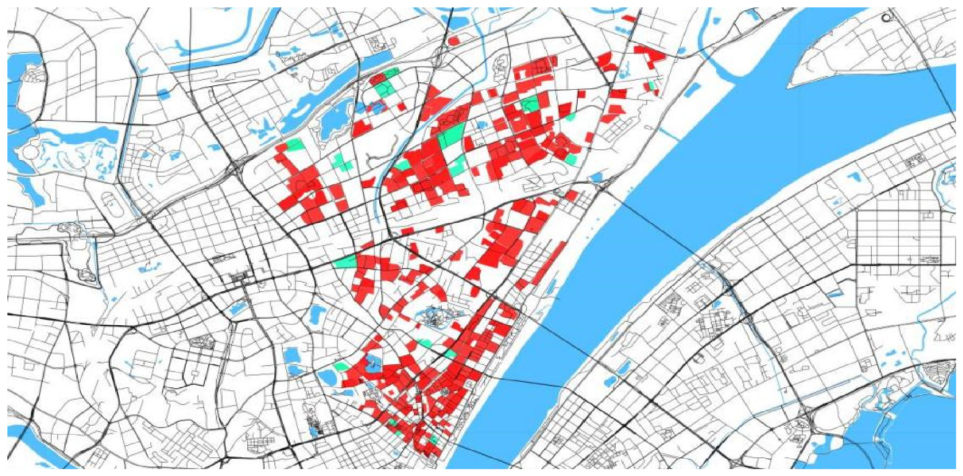
As illustrated in Figure 9, this study used the parametric platform Grasshopper to extract three-dimensional building data for 285 residential blocks in the Hankou district of Wuhan (specifically the Qiaokou, Jianghan, and Jiangan districts) based on SHP and DBF files. This study randomly split the 285 blocks into 265 blocks and 20 blocks, the data from 265 residential blocks (red) were used for the GNN model training phases, and the remaining 20 blocks (cyan) were reserved as an independent set for the model energy consumption predictions validation. The 265 blocks, in training phases, were divided based on a 70/30 ratio: 186 blocks (70.2%) were used for training, and 79 blocks (29.8%) were used for testing.

Figure 9. The visualization of 285 residential blocks.

As detailed in Table 13, heterogeneous graph structures and their corresponding datasets were generated for each block using parametric methods. Concurrently, node morphology features and edge features were derived using the same parametric framework. The energy simulations were conducted for each building node within 285 blocks.

Table 13. Visualization of the layout and heterogeneous diagrams of the blocks.

Block Number	The Building Layout	The Heterogeneous Graph
29
128
214

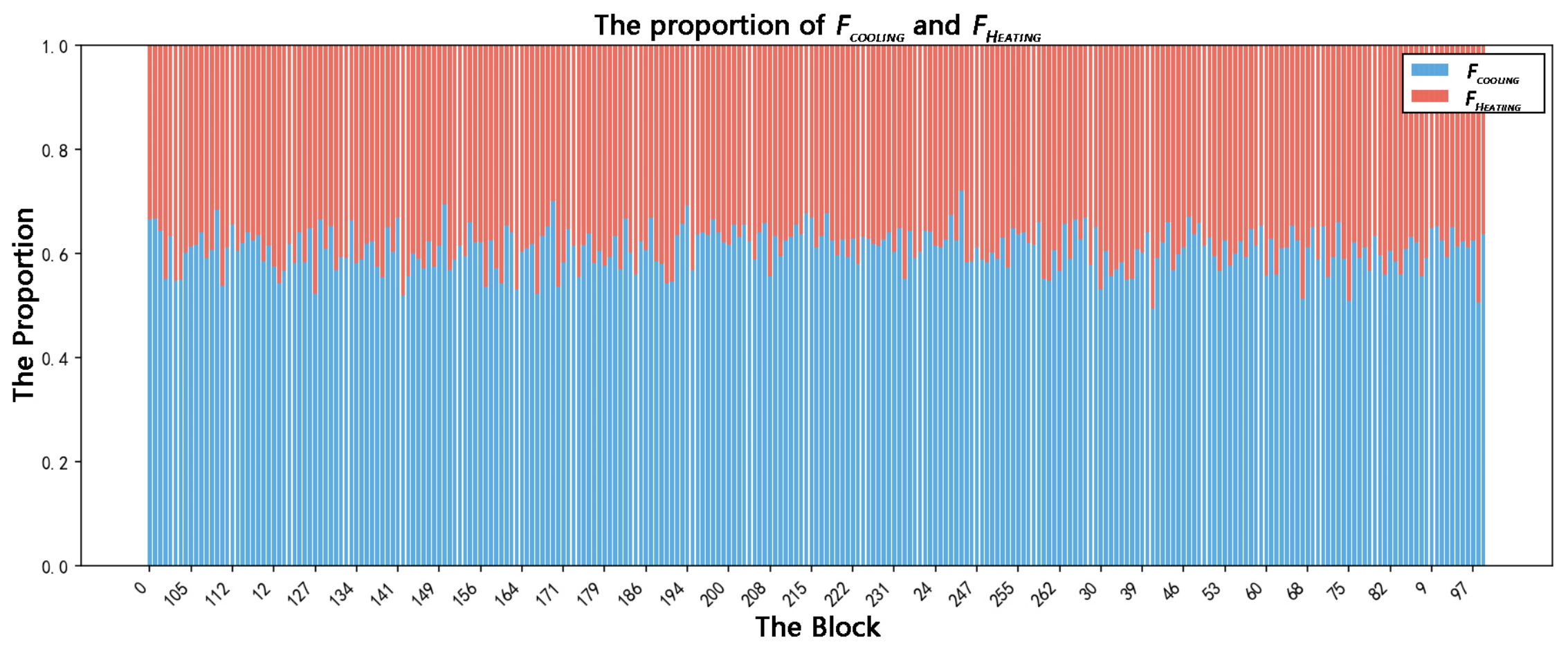
As shown in Figure 10, the simulated $F_{Cooling}$ of the building nodes was significantly higher than $F_{Heating}$, which aligns with the typical energy consumption patterns of residential buildings in Wuhan. Both the simulated summer-cooling and winter-heating energy values were subsequently integrated into the GNN model as node energy features.

Figure 10. The $F_{Cooling}$ and $F_{Heating}$ visualization.

3.2. The GNN Model Selection and Performance Evaluation

3.2.1. Hyperparameter Optimization Results

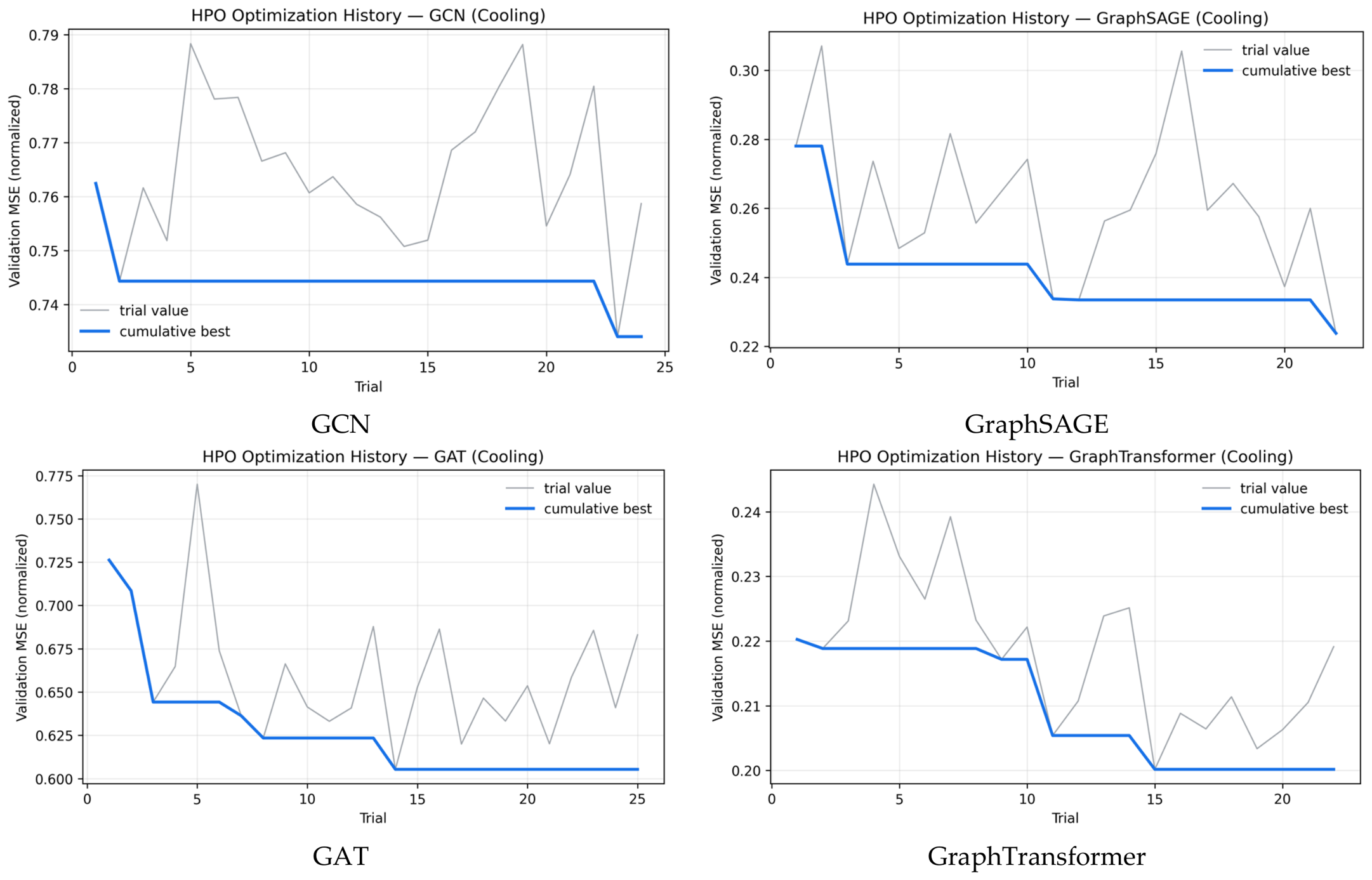
In this study, hyperparameter optimization (HPO) was performed on the four GNN encoders using Optuna, with the minimum MSE loss serving as the objective function. Table 14 shows the best hyperparameter configurations found for each model after the HPO process. As shown in Figure 11, the results indicate that the GraphTransformer achieved the lowest MSE value (0.200168), followed by GraphSAGE (0.223806), suggesting these models are better suited for the heterogeneous urban block dataset.

Table 14. Optimal hyperparameter configurations.

Hyperparameter	GCN	GAT	GraphSAGE	GraphTransformer
Record trials	30	30	30	30
Best MSE	0.734026	0.605352	0.223806	0.200168
Learning rate	5.6388 × 10−4	0.00596	4.8391 × 10−4	0.001133
Weight decay	5.3846 × 10−4	1.8619 × 10−4	0.001848	4.1643 × 10−5
Dropout	0.2432	0.17523	0.201166	0.1278
No. of layers	4	4	4	2
Hidden dim	{256, 128, 32, 8}	{64, 32, 32, 16}	{256, 128, 16, 8}	{256, 256}
Heads	None	{8, 4, 2}	None	8

Figure 11. The HPO optimization history of four GNN algorithms.

3.2.2. GNN Models’ Training

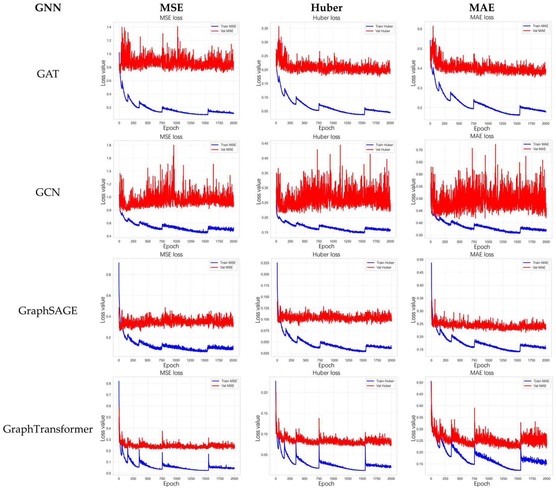
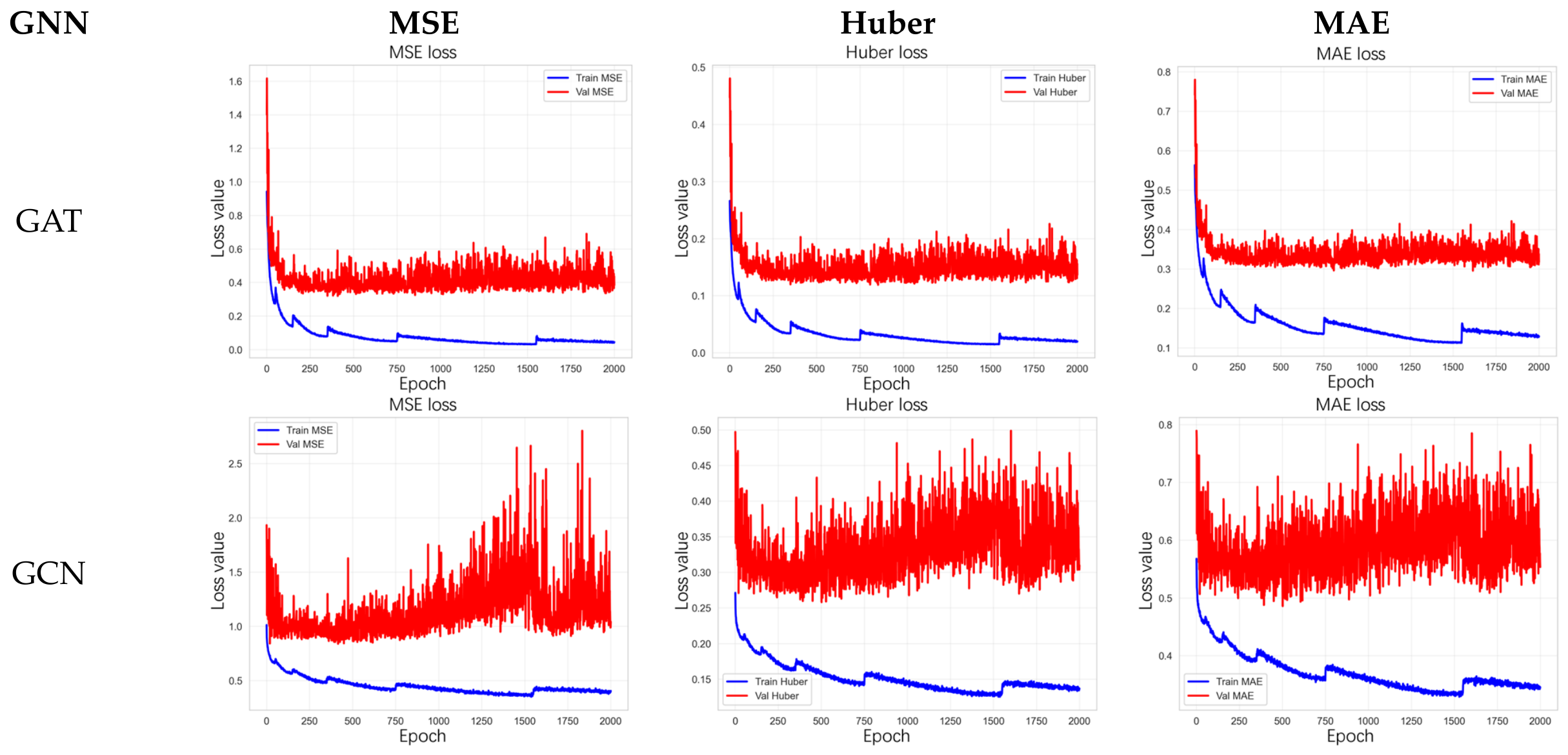
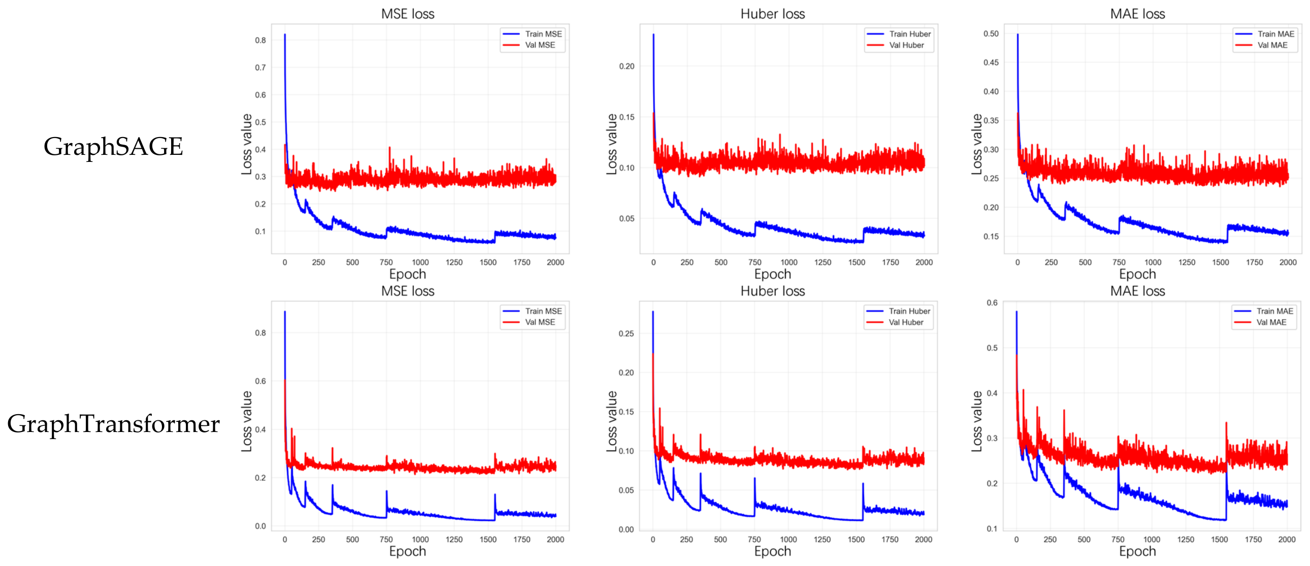
Figure 12 and Figure 13 illustrate the training loss trajectories of the four GNN algorithms for the two target features ($F_{Cooling}$ and $F_{Heating}$). All models were trained for a total of 2000 epochs to ensure full convergence. The best model for each architecture was selected based on the minimum, ${Loss}_{MSE}$, recorded in the validation set.

Figure 12. The ${\mathrm{F}}_{\mathrm{C}\mathrm{o}\mathrm{o}\mathrm{l}\mathrm{i}\mathrm{n}\mathrm{g}}$ training loss visualization.

Figure 13. The ${\mathrm{F}}_{\mathrm{H}\mathrm{e}\mathrm{a}\mathrm{t}\mathrm{i}\mathrm{n}\mathrm{g}}$ training loss visualization.

As summarized in Table 15 and Table 16, GraphSAGE and GraphTransformer demonstrated the highest performance for both targets. The validation MSE for these algorithms reached 0.208–0.256 for $F_{Cooling}$ and 0.213–0.246 for $F_{Heating}$, exhibiting a superior predictive accuracy compared to GCN and GAT.

Table 15. Performance for $F_{Cooling}$ prediction.

GNN Algorithm	Dataset	MSE Loss	Huber Loss	MAE Loss
GAT	Train/Val	0.640/0.709	0.183/0.218	0.411/0.437
GCN	Train/Val	0.645/0.779	0.184/0.215	0.413/0.427
GraphSAGE	Train/Val	0.152/0.256	0.057/0.086	0.198/0.220
GraphTransformer	Train/Val	0.027/0.208	0.014/0.070	0.129/0.218

Table 16. Performance for $F_{Heating}$ prediction.

GNN Algorithm	Dataset	MSE Loss	Huber Loss	MAE Loss
GAT	Train/Val	0.097/0.319	0.041/0.123	0.181/0.313
GCN	Train/Val	0.491/0.838	0.164/0.273	0.393/0.529
GraphSAGE	Train/Val	0.133/0.246	0.052/0.091	0.193/0.248
GraphTransformer	Train/Val	0.046/0.213	0.023/0.077	0.162/0.232

The unsatisfactory performance of GCN can be attributed to its spectral convolution mechanism. As the depth of the graph increases, the global aggregation process often fails to effectively distinguish the features of the building nodes, resulting in over-smoothing [68]. In contrast, GraphSAGE addresses this through sampling and aggregation methods, thereby effectively preserving the heterogeneity data of energy consumption [69]. Moreover, the GraphTransformer has shown superior performance compared to GAT, attributable to its global attention mechanism, which effectively captures long-range dependencies among all nodes concurrently [70]. Conversely, the local attention of GAT focuses only on direct neighbors, limiting its ability to use the global spatial context of the urban layout. By integrating positional encoding, the GraphTransformer overcomes these local constraints, facilitating a more accurate modeling of complex spatial interactions. The final models are shown in Table 17.

Table 17. Final best models for energy prediction.

Target	Rank	Algorithm	Best Epoch	Val MSE
${\mathrm{F}}_{\mathrm{H}\mathrm{e}\mathrm{a}\mathrm{t}\mathrm{i}\mathrm{n}\mathrm{g}}$	1	GraphTransformer	916	0.213
	2	GraphSAGE	259	0.246
${\mathrm{F}}_{\mathrm{C}\mathrm{o}\mathrm{o}\mathrm{l}\mathrm{i}\mathrm{n}\mathrm{g}}$	1	GraphTransformer	1328	0.208
	2	GraphSAGE	382	0.256

3.3. Evaluation and Validation of GNN Models

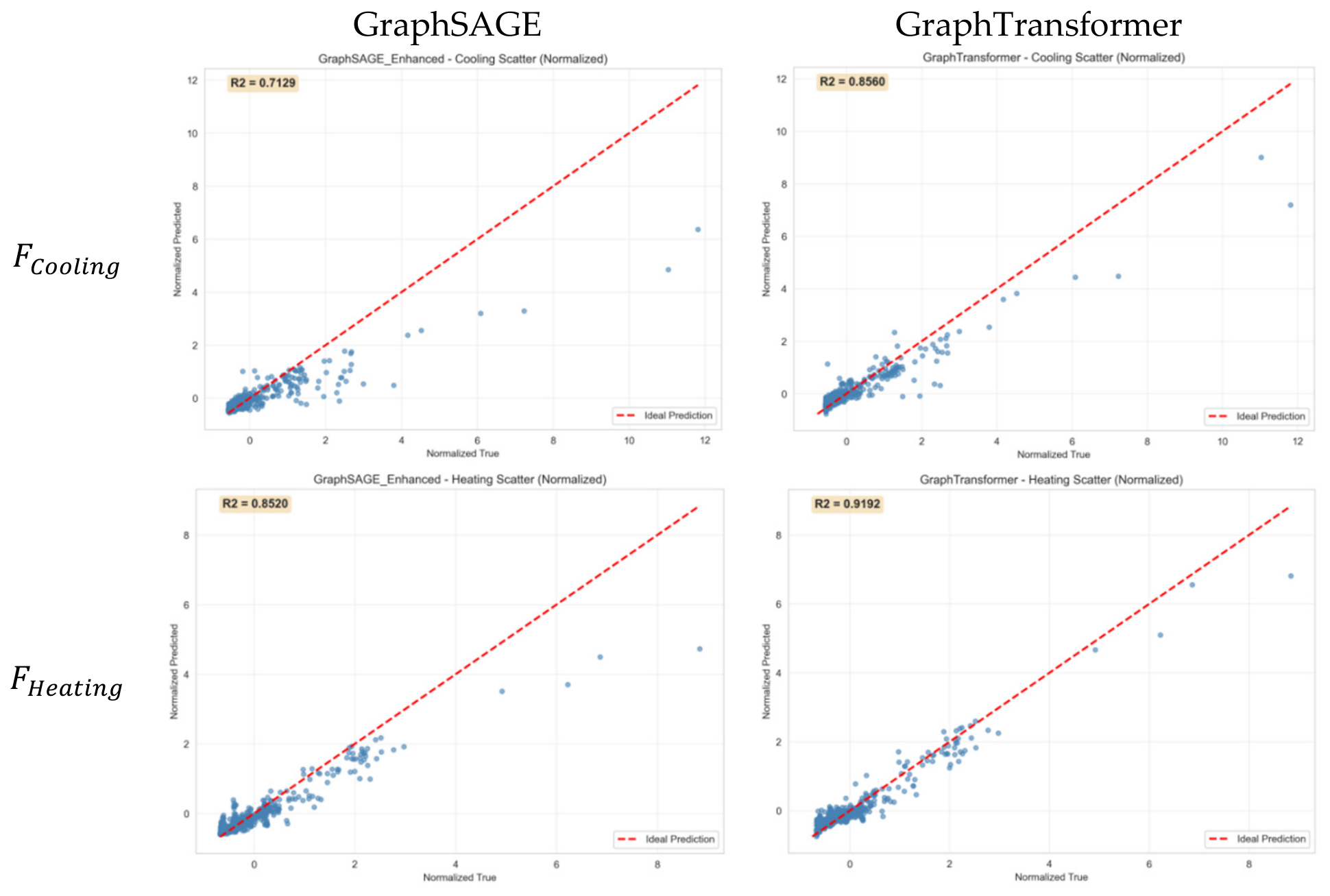
To verify the robustness of the framework, the final GNN models were used to predict the energy consumption of 20 independent blocks in the final validation dataset. A comparative analysis between the GNN-predicted values and the simulated ground truth for all building nodes in these blocks was made, as illustrated in Figure 14. The key findings are as follows:

Figure 14. Scatter plot of GNN prediction model on the validation dataset.

• $F_{Cooling}$: The GraphTransformer model showed superior predictive capability, with an ${\mathrm{R}}^2$ of 0.8560, while the GraphSAGE model showed strong performance, with an ${\mathrm{R}}^2$ of 0.7129.
• $F_{Heating}$: The GraphTransformer model performed exceptionally well, achieving an ${\mathrm{R}}^2$ value of 0.9192. Similarly, the GraphSAGE model exhibited a strong performance, with an ${\mathrm{R}}^2$ of 0.8520.

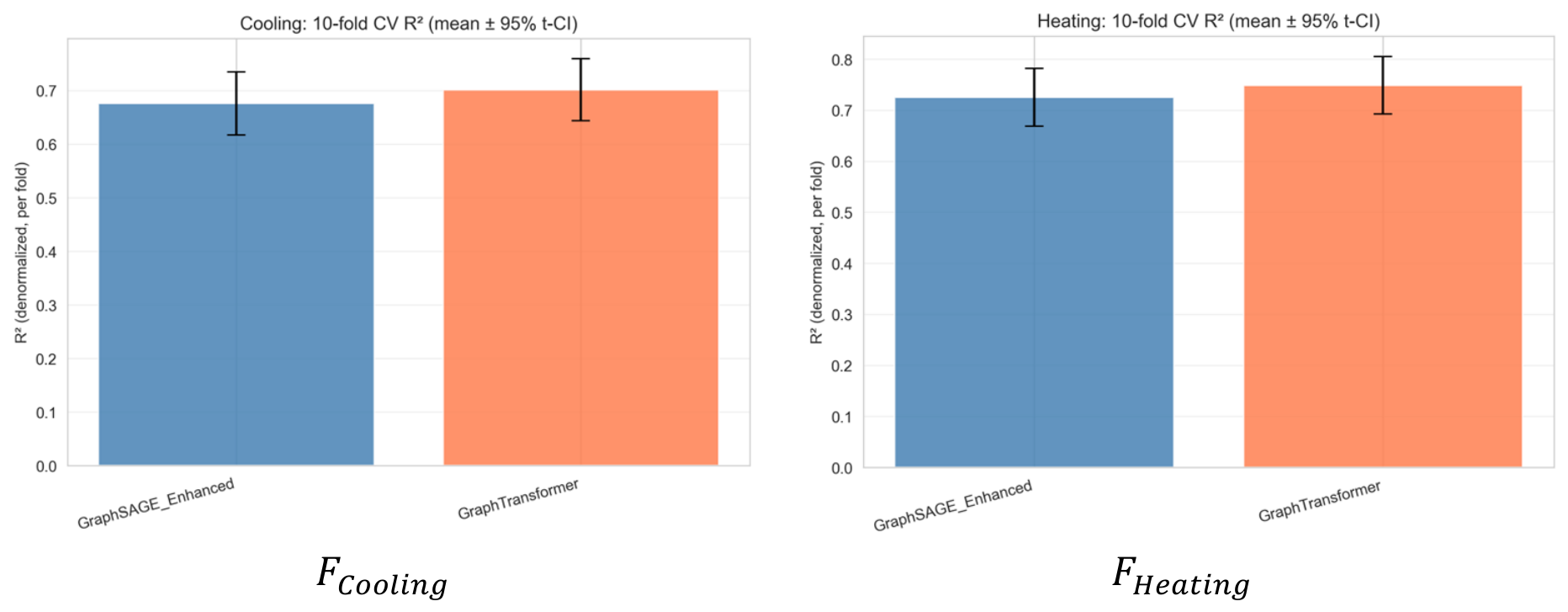
To evaluate the generalization performance of the GNN models, a 10-fold cross-validation approach was implemented. Data from 265 blocks were randomly partitioned into 10 subsets, where each fold served as the validation set, while the remaining folds formed the training set. GNN models based on GraphSAGE and GraphTransformer were trained separately for $F_{Cooling}$ and $F_{Heating}$, as with the training framework described previously. Model performance on the validation sets was evaluated by calculating the $R^2$ value between the predicted and simulated values of the block nodes. As illustrated in Figure 15, the mean $R^2$ values, alongside their 95% confidence intervals (CIs), were computed for both models. This study found the following:

Figure 15. Ten-fold cross-validation for $F_{Cooling}$ and $F_{Heating}$.

• $F_{Cooling}$: GraphTransformer achieved a mean $R^2$ of 0.701 (95% CI: [0.644, 0.759]), and GraphSAGE achieved 0.676 (95% CI: [0.617, 0.735]). The result shown a marginal superiority of GraphTransformer for $F_{Cooling}$ prediction.
• ${\mathrm{F}}_{\mathrm{H}\mathrm{e}\mathrm{a}\mathrm{t}\mathrm{i}\mathrm{n}\mathrm{g}}$: GraphTransformer obtained a mean R² of 0.749 (95% CI: [0.693, 0.805]), compared to 0.72 5 (95% CI: [0.669, 0.782]) for GraphSAGE.

Generally, prediction accuracy was higher for ${\mathrm{F}}_{\mathrm{H}\mathrm{e}\mathrm{a}\mathrm{t}\mathrm{i}\mathrm{n}\mathrm{g}}$ than for $F_{Cooling}$. However, the performance gap between the two models remained narrow, with GraphTransformer again slightly outperforming GraphSAGE.

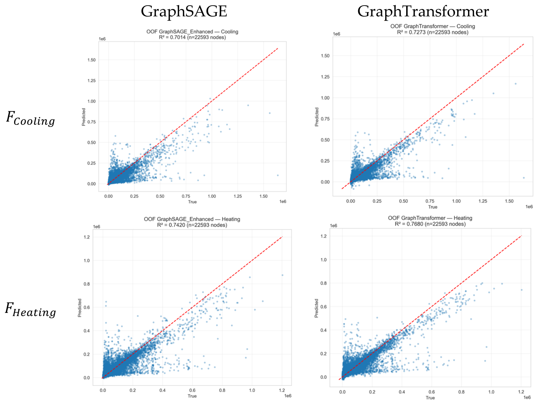
Alternatively, out-of-fold (OOF) analyses were evaluated by aggregating the GNN predictions and simulated values across all validation sets from the cross-validation process. The $R^2$ values were then computed across all validation nodes within the 10 datasets. As shown in Figure 16, the analysis revealed the following:

Figure 16. OOF scatter plot of GNN prediction model.

• $F_{Cooling}$: GraphTransformer achieved an $R^2$ of 0.727, better than GraphSAGE, which has an $R^2$ of 0.701, showing superior performance in $F_{Cooling}$ prediction.
• $F_{Heating}:$ GraphTransformer achieved an R² of 0.768, whereas GraphSage reached 0.742.

These findings confirm that the models of $\mathrm{G}\mathrm{r}\mathrm{a}\mathrm{p}\mathrm{h}\mathrm{T}\mathrm{r}\mathrm{a}\mathrm{n}\mathrm{s}\mathrm{f}\mathrm{o}\mathrm{r}\mathrm{m}\mathrm{e}\mathrm{r}$ and $\mathrm{G}\mathrm{r}\mathrm{a}\mathrm{p}\mathrm{h}\mathrm{S}\mathrm{A}\mathrm{G}\mathrm{E}$ are good for both ${\mathrm{F}}_{\mathrm{C}\mathrm{o}\mathrm{o}\mathrm{l}\mathrm{i}\mathrm{n}\mathrm{g}}$ and ${\mathrm{F}}_{\mathrm{H}\mathrm{e}\mathrm{a}\mathrm{t}\mathrm{i}\mathrm{n}\mathrm{g}}$ prediction tasks.

Generally, both GNN algorithms achieved good prediction results in the two energy consumption aspects, thus indicating that the two GNN prediction models can be applied to the block energy consumption prediction task in Wuhan City. The GraphTransformer algorithm outperformed GraphSAGE in both energy consumption aspects.

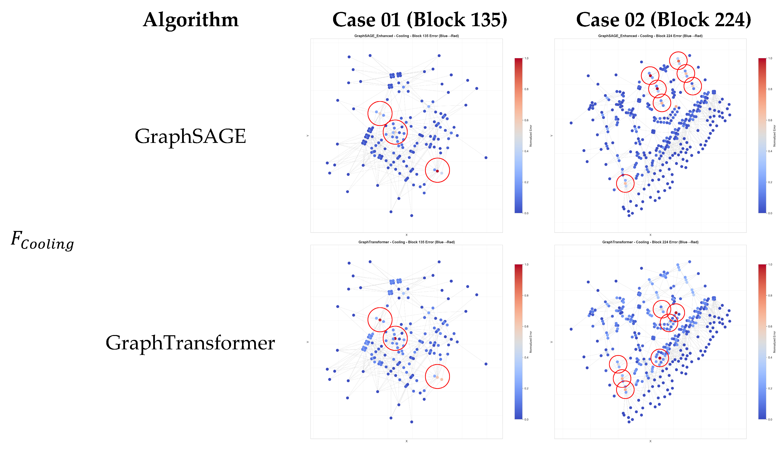
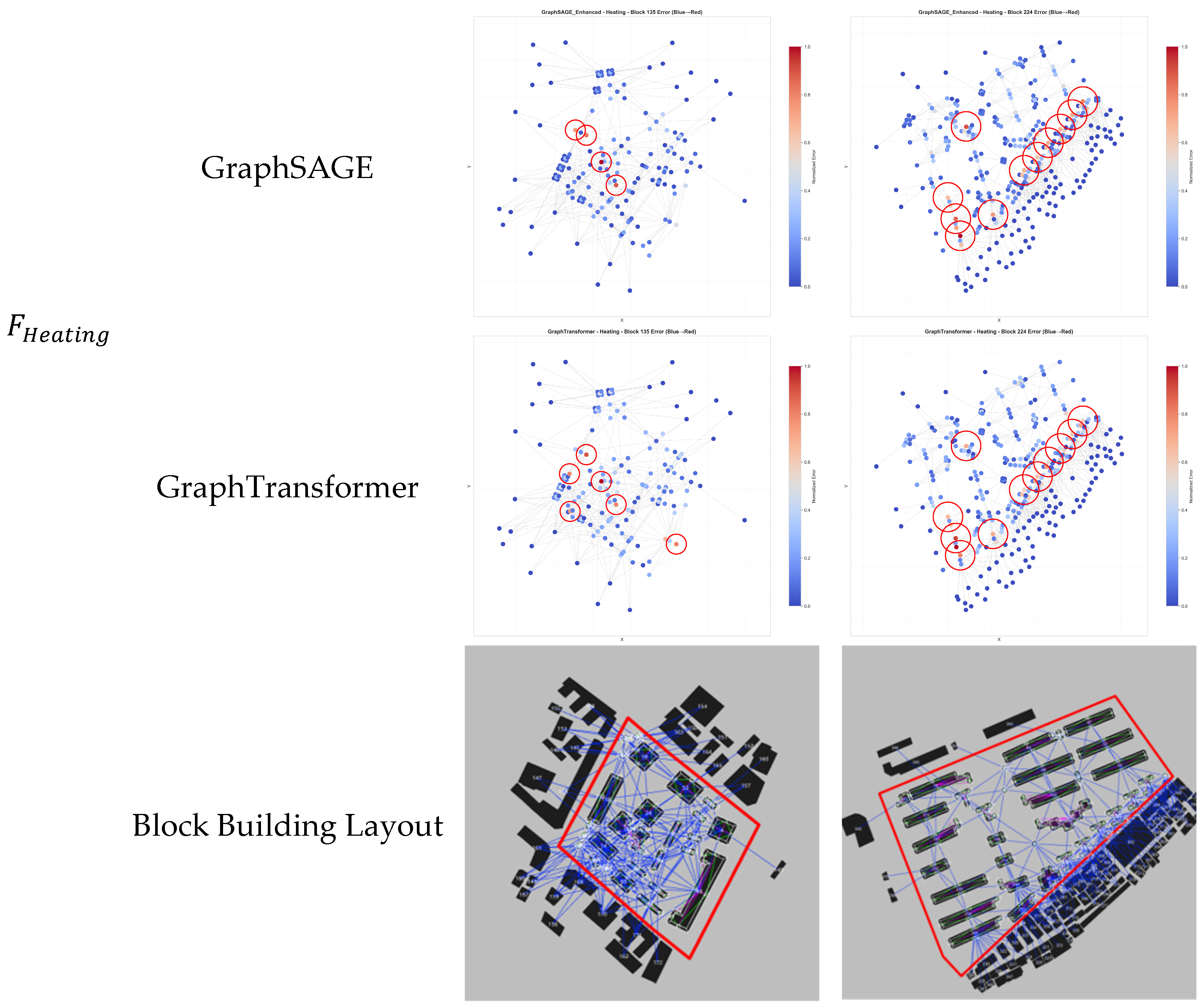
The spatial distribution of prediction errors of $F_{Cooling}$ and $F_{Heating}$ for both GNN algorithms was analyzed. As illustrated in Figure 17, the $F_{Cooling}$ error patterns in Case 01 and Case 02 have differences between the two models. On the other hand, the $F_{Heating}$ errors showed a consistent spatial trend for both algorithms. This study found the following:

Figure 17. Visualization of prediction errors in GNN models.

• In terms of $F_{Cooling}$, both GraphSAGE and GraphTransformer displayed similar error distributions in Case 01, with inaccuracies mainly concentrated in the central zone of the buildings near to the centroid of the block. In Case 02, the error distributions of two models have differences: the errors of GraphSAGE were largely found in the central zones of the northern building, while the errors were found more in the central zones of buildings along the block southern boundary in the GraphTransformer model. In Case 01, two nodes in the GraphTransformer predictions (1.6% of the 122 total nodes) and one node in the GraphSAGE predictions (0.8% of 122 nodes) exhibited extreme errors exceeding 80%; notably, all three nodes are building ${\mathrm{Z}\mathrm{o}\mathrm{n}\mathrm{e}}_0$ nodes. Similarly, in Case 02, both GraphSAGE and GraphTransformer generated errors above 80% at two nodes (0.96% of the 208 total nodes), with these nodes consistently localized at building ${\mathrm{Z}\mathrm{o}\mathrm{n}\mathrm{e}}_0$ nodes.
• In terms of $F_{Heating}$, both models showed highly consistent error distributions in all cases. In Case 01, errors were mainly located in the southwest buildings; in Case 02, the errors shifted to the southeast street-facing buildings. In Case 01, extreme prediction errors exceeding 80% occurred at four nodes for the GraphTransformer (3.2% of the 122 total nodes) and two nodes for GraphSAGE (1.6% of 122 nodes), with all nodes localized at ${\mathrm{Z}\mathrm{o}\mathrm{n}\mathrm{e}}_0$ nodes. Similarly, in Case 02, such high errors were observed at six nodes in GraphSAGE (2.88% of the 208 total nodes) and four nodes in GraphTransformer (1.92% of 208 nodes); notably, this prediction failure remained consistently concentrated in the building ${\mathrm{Z}\mathrm{o}\mathrm{n}\mathrm{e}}_0$ nodes.

In summary, while both cases contained nodes with errors exceeding 80% (less than 5% of the total dataset), fewer than 10% of the nodes had errors over 40%. The errors exceeding 80% were mainly localized at building ${\mathrm{Z}\mathrm{o}\mathrm{n}\mathrm{e}}_0$ nodes. From a physical and topological perspective, ${\mathrm{Z}\mathrm{o}\mathrm{n}\mathrm{e}}_0$ nodes are geometrically encapsulated by surrounding zones, resulting in minimal direct shading from other buildings. Consequently, the GNN models hardly capture their thermal conditions without the BLG topology.

The distribution analysis results suggest that the energy prediction accuracy of these algorithms is sensitive to the urban context. In Case 01, errors were concentrated in the center of the block, where shading effects are dominated by internal southern buildings. On the other hand, in Case 02, numerous buildings located in the south boundary of the block create significant shading for the southern buildings in the block, shifting the error concentration to that area. This study also found that the high errors mainly in the central zone of buildings in all scenarios suggest that these areas―being heavily influenced by neighboring zones―present a greater challenge for accurate energy prediction [71].

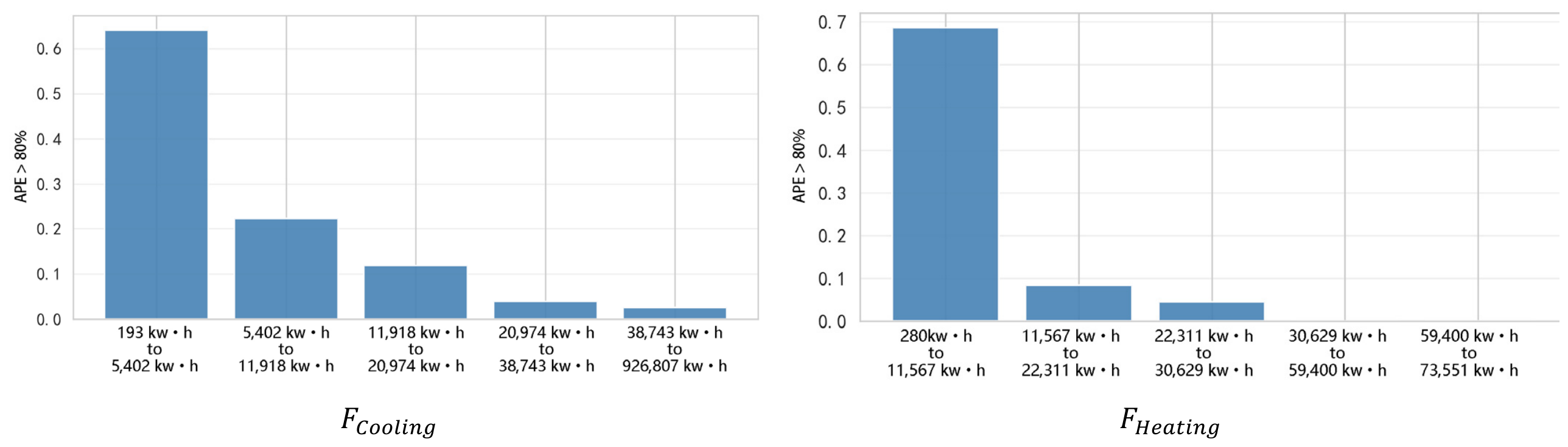
To investigate error distribution, the simulated ${\mathrm{F}}_{\mathrm{C}\mathrm{o}\mathrm{o}\mathrm{l}\mathrm{i}\mathrm{n}\mathrm{g}}$ and ${\mathrm{F}}_{\mathrm{H}\mathrm{e}\mathrm{a}\mathrm{t}\mathrm{i}\mathrm{n}\mathrm{g}}$ values of all block nodes within the independent dataset were sorted in ascending order. These nodes were then partitioned into five groups of approximately equal size based on their simulated values. The Absolute Percentage Error (APE) for each node was calculated using Equation (23), based on the GraphTransformer predicted value (${\mathrm{V}\mathrm{a}\mathrm{l}\mathrm{u}\mathrm{e}}_{\mathrm{p}\mathrm{r}\mathrm{e}\mathrm{d}}$) and simulation value (${\mathrm{V}\mathrm{a}\mathrm{l}\mathrm{u}\mathrm{e}}_{\mathrm{s}\mathrm{i}\mathrm{m}}$). The proportion of nodes with an APE exceeding 80% was subsequently quantified for each group. As illustrated in Figure 18, the analysis revealed the following patterns:

Figure 18. APE analysis for GraphTransformer models.

• $F_{Cooling}$: In the lowest $F_{Cooling}$ group (193 to 5402 kWh), 60% of the nodes exhibited an APE greater than 80%. This proportion decreased to approximately 20% in the medium group (11,018 to 20,974 kWh) and dropped to nearly 0.1% in the two highest consumption groups.
• $F_{Heating}$: For the lowest $F_{Heating}$ group (280 to 11,567 kWh), the proportion of nodes with an APE exceeding 80% reached 65%. This rate fell below 10% in the medium group (22,311 to 30,629 kWh) and approached 0% in the two highest consumption groups.

The APE analysis indicates that the prediction errors of the GraphTransformer model are mainly concentrated in low-energy consumption nodes. Because the simulated values for these nodes are small, even minor deviations in predictions inflate the APE. Conversely, GraphTransformer shows high predictive accuracy for high-energy consumption nodes.

$$APE\left(\%\right)= {\displaystyle \frac{\left|{Value}_{pred}-{Value}_{sim}\right|}{\left|{Value}_{sim}\right|}}\times 100$$

(23)

4. Discussion

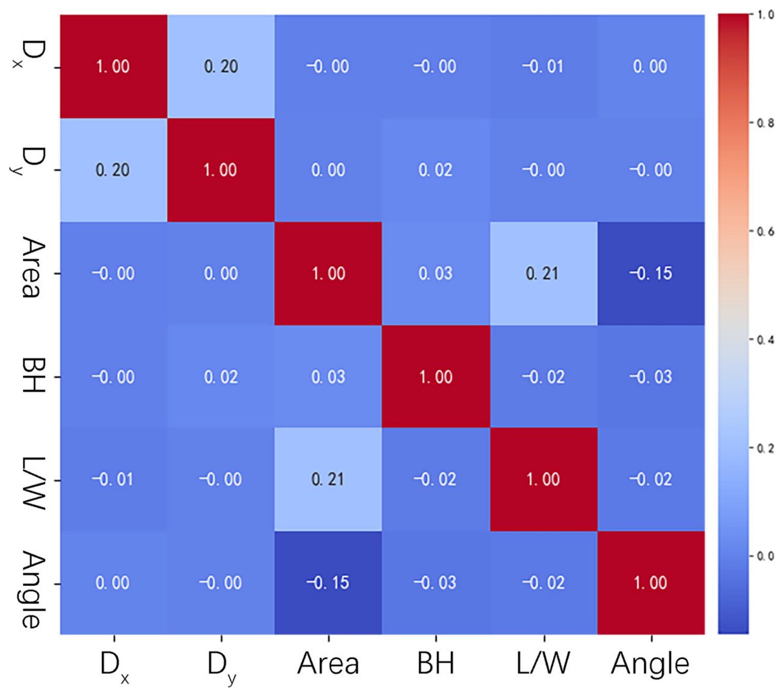
Before the GNN interpretability analysis, this study made a correlation analysis of the features for each node. As shown in Figure 19, there is no strong correlation among the six features of the nodes.

Figure 19. Pearson correlation analysis.

To show the operational mechanisms of the GNN predictive models, this study used GNNExplainer to perform a comparative analysis of the GraphSAGE and GraphTransformer models. This section explores the prediction logic of the surrogate models through the node feature importance and edge-level signal-propagation patterns.

4.1. Node Feature Importance Analysis

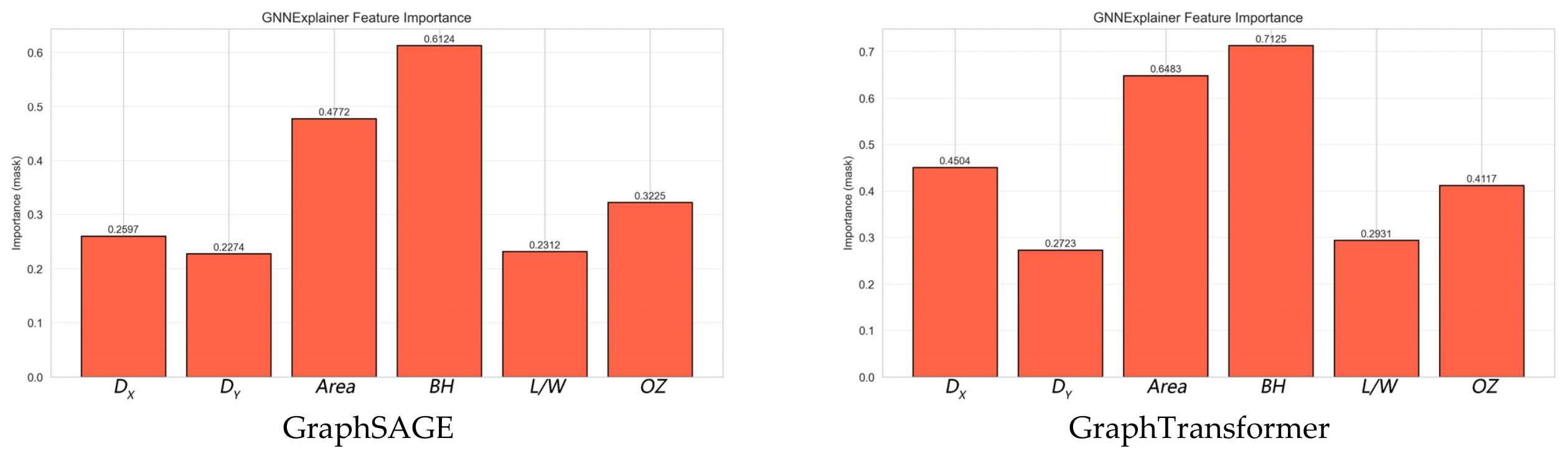
As shown in Figure 20, $BH$ (0.6124 for GraphSAGE and 0.7125 for GraphTransformer) and $Area$ (0.4772 for GraphSAGE and 0.6483 for GraphTransformer) are the most critical node features in $F_{Cooling}$ prediction. Physically, increased building height correlates with a lower shape factor, which minimizes the envelope-to-volume ratio and subsequently reduces unit-area heat-gain and cooling-system energy consumption. Conversely, a larger floor area necessitates higher cooling capacities and extended operational hours to maintain cooling-system setpoint, thereby increasing cooling-system energy consumption. The $D_x$ (representing east–west positioning) exhibited high importance in the GraphTransformer model (0.4504). This suggests that the model more effectively captures how east–west direction building layout distribution influences inter-building shading [20] and the subsequent cooling energy demand. Finally, $OZ$ was identified as a critical feature (0.3225 and 0.4117), confirming that GNN algorithms prioritize the orientation of facade relative to the south, where minimized angles with north direction mean higher solar gains.

Figure 20. The $F_{Cooling}$ GNN node feature importance.

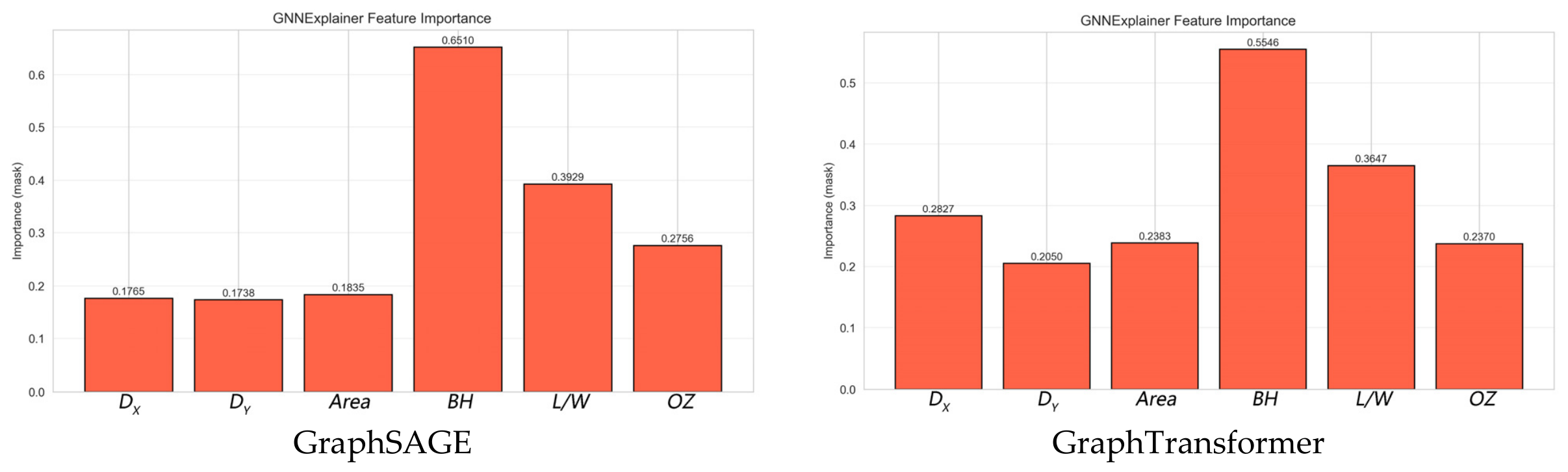
As shown in Figure 21, both models emphasized $BH$ (0.651 and 0.576) and $L/W$ (0.393 and 0.372) as key indicators in $F_{Heating}$ prediction. Like $F_{Heating}$, an increased height reduces the shape factor and unit-volume heat loss, thereby decreasing $F_{Heating}$. A higher $L/W$ increases the exposure surface area of buildings, thereby accelerating heat dissipation and increasing $F_{Heating}$. Furthermore, $D_x$ is also an important feature in GraphTransformer for $F_{Heating}$ prediction. This suggests that the model more effectively captures how east–west direction building layout distribution influences inter-building shading and the subsequent heating energy demand.

Figure 21. The $F_{Heating}$ GNN node feature importance.

In summary, this study identifies $BH$, $Area$, $L/W$, and $D_x$ as the important features governing urban block energy consumption. These indicators exhibit a significant coupling with the “hot-summer and cold-winter” climate characteristics of Wuhan:

• Scale effect: $BH$ and $Area$ describe total building volume and envelope surface area. Under the extreme summer-cooling and winter-heating demands of Wuhan, HVAC loads positive with the building volume.
• Solar shading: $L/W$ and $D_x$ describe inter-building shading dynamics and solar heat gain. During Wuhan’s high-radiation summer, elevated $BH$ and $L/W$ values maximize individual envelope exposure while simultaneously generating shading that effectively reduces the summer cooling load and increases the winter heating load of neighborhood buildings. Furthermore, $D_x$ reflects the longitudinal positioning of buildings, fundamentally altering the penetration of southern solar radiation into the block. This dynamic trade-off between summer shading and winter heat gain establishes the core value of morphological optimization in hot-summer and cold-winter zones.

4.2. Edge Propagation and Message-Passing Patterns

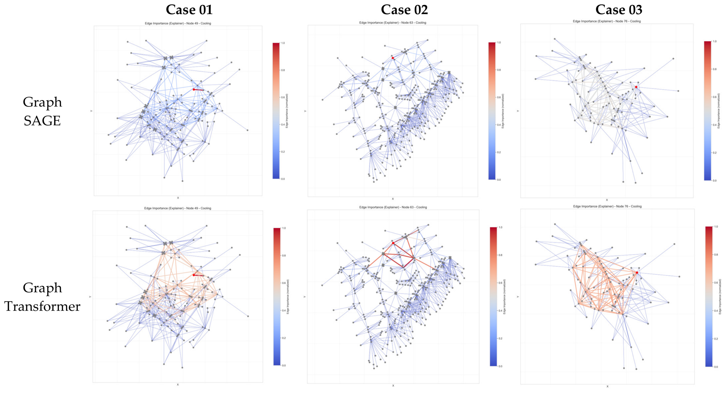
As shown in Figure 22, the visualization of the explanation graphs for $F_{Cooling}$ prediction reveals fundamental differences in how these algorithms identify urban topology:

Figure 22. The message-passing patterns of $F_{Cooling}$ GNN models.

• Case 1: For the target node prediction, GraphSAGE used only a single adjacent edge. In contrast, GraphTransformer used a substantial cluster of edge relationships from the southwestern direction, capturing a broader spatial context.
• Case 2: GraphSAGE failed to incorporate surrounding edge relationships. Conversely, GraphTransformer successfully identified and used critical edges located to the south of the target node, reflecting the impact of southern solar shading.
• Case 3: Although both models recognized southwestern edge influences, GraphTransformer assigned significantly higher influence weights to these connections.

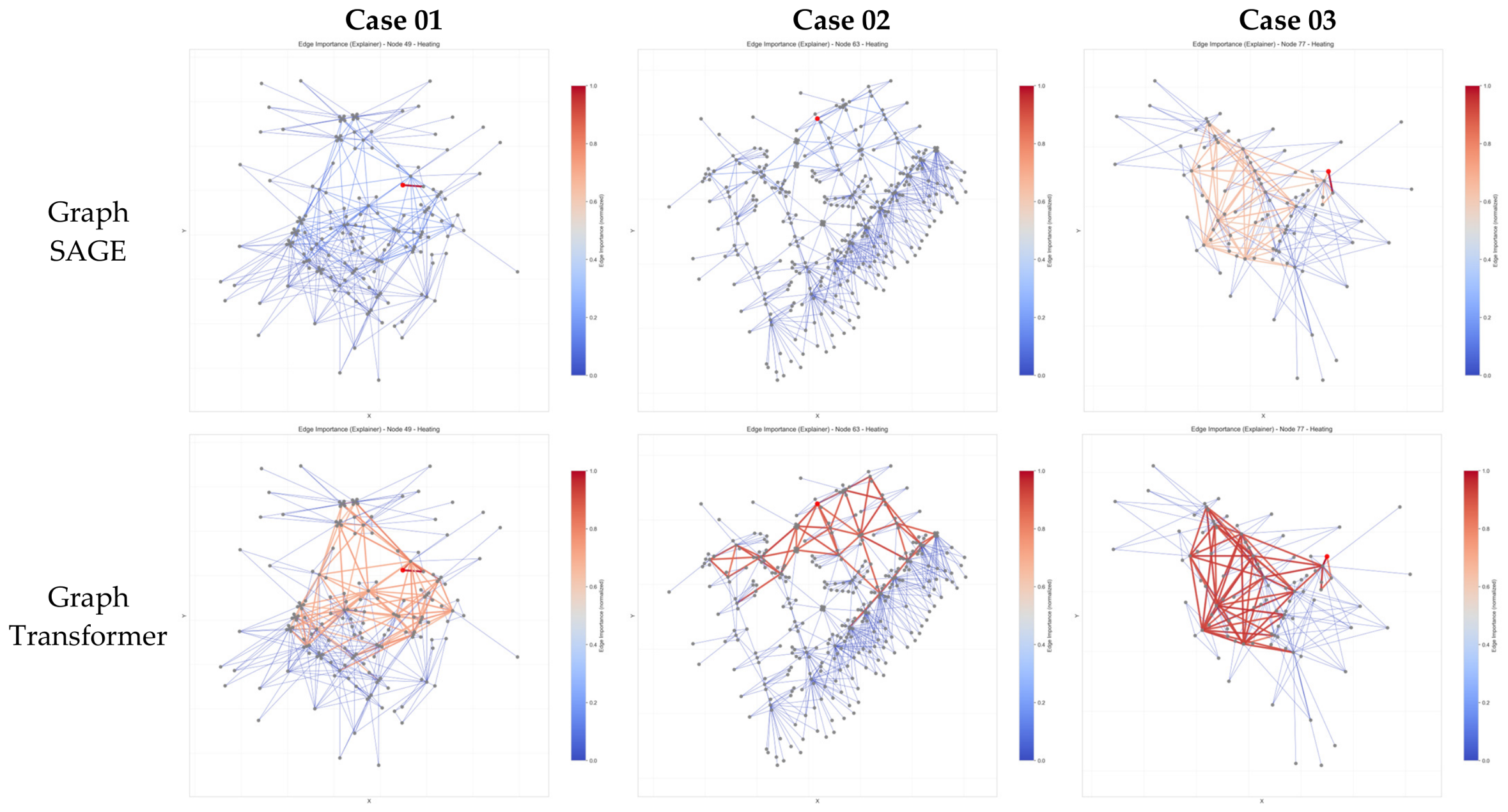
As shown in Figure 23, the visualization of the explanation graphs for $F_{Heating}$ prediction reveals fundamental differences in how these algorithms identify urban topology:

Figure 23. The message-passing patterns of $F_{Heating}$ GNN models.

• Case 1: GraphSAGE focused on a single adjacent signal, while GraphTransformer incorporated extensive signals from the surroundings and the southwest.
• Case 2: GraphSAGE failed to incorporate surrounding edge relationships, whereas GraphTransformer successfully used extensive southern edge signals.
• Case 3: Both models utilized similar signals, but GraphTransformer demonstrated a higher sensitivity to these topological inputs by increased signal weights.

In summary, the two algorithms exhibit a shared reliance on $Area$ and $BH$ as core indicators. However, a significant difference exists in their utilization of spatial context: GraphTransformer uniquely incorporates $D_x$ as a critical node feature and consistently uses southward and westward edge signals to inform its predictions. This suggests that GraphTransformer possesses a better ability to internalize the physical shading logic in urban layouts than GraphSAGE.

4.3. GNNExplainer Stability Analysis

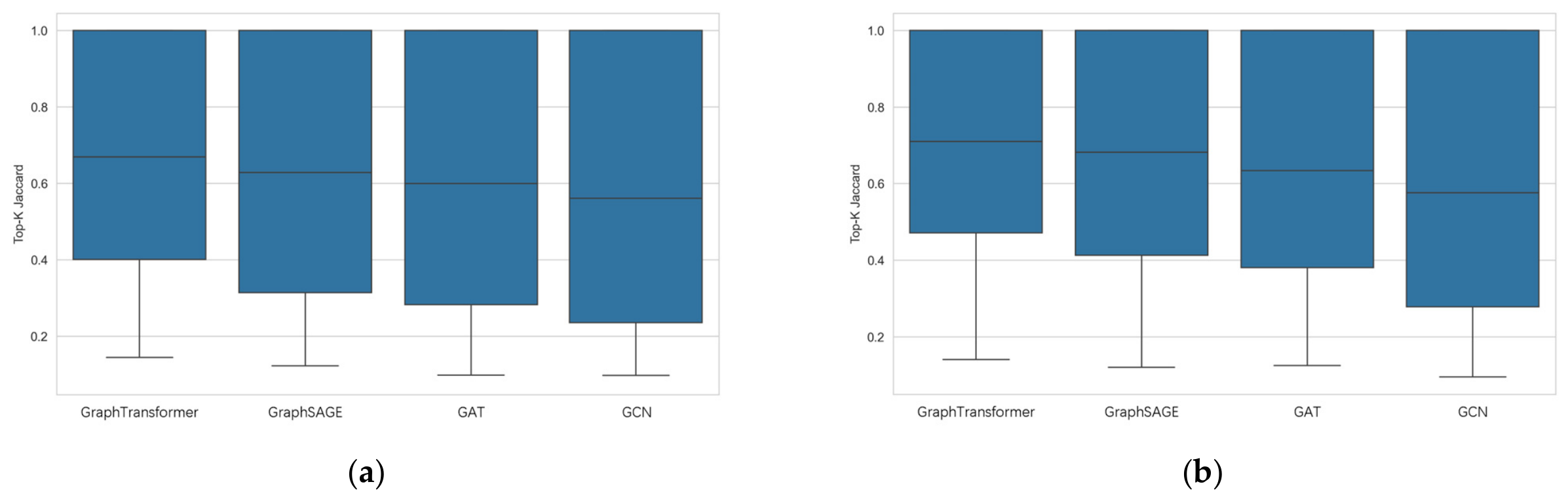
As shown in Figure 24, the post hoc explanation stability of GNNExplainer across both $F_{Cooling}$ and $F_{Heating}$ exhibits a highly consistent architectural hierarchy, ordered as follows: GraphTransformer > GraphSAGE > GAT > GCN.

Figure 24. The GNNExplainer stability analysis ((a) $F_{Cooling}$ and (b) $F_{Heating}$).

Notably, the explanation reliability for all models scales is slightly higher in $F_{Heating}$, with the GraphTransformer reaching a peak median Jaccard similarity of 0.71 compared to $F_{Cooling}$ (0.67). This cross-seasonal consistency establishes that the multi-head self-attention mechanism within the GraphTransformer inherently extracts more deterministic, invariant edge-level structural features that remain resilient against random initialization seeds, thereby providing significantly more trustworthy interpretations for building energy prediction than traditional localized message-passing networks.

4.4. GNN Ablation Study

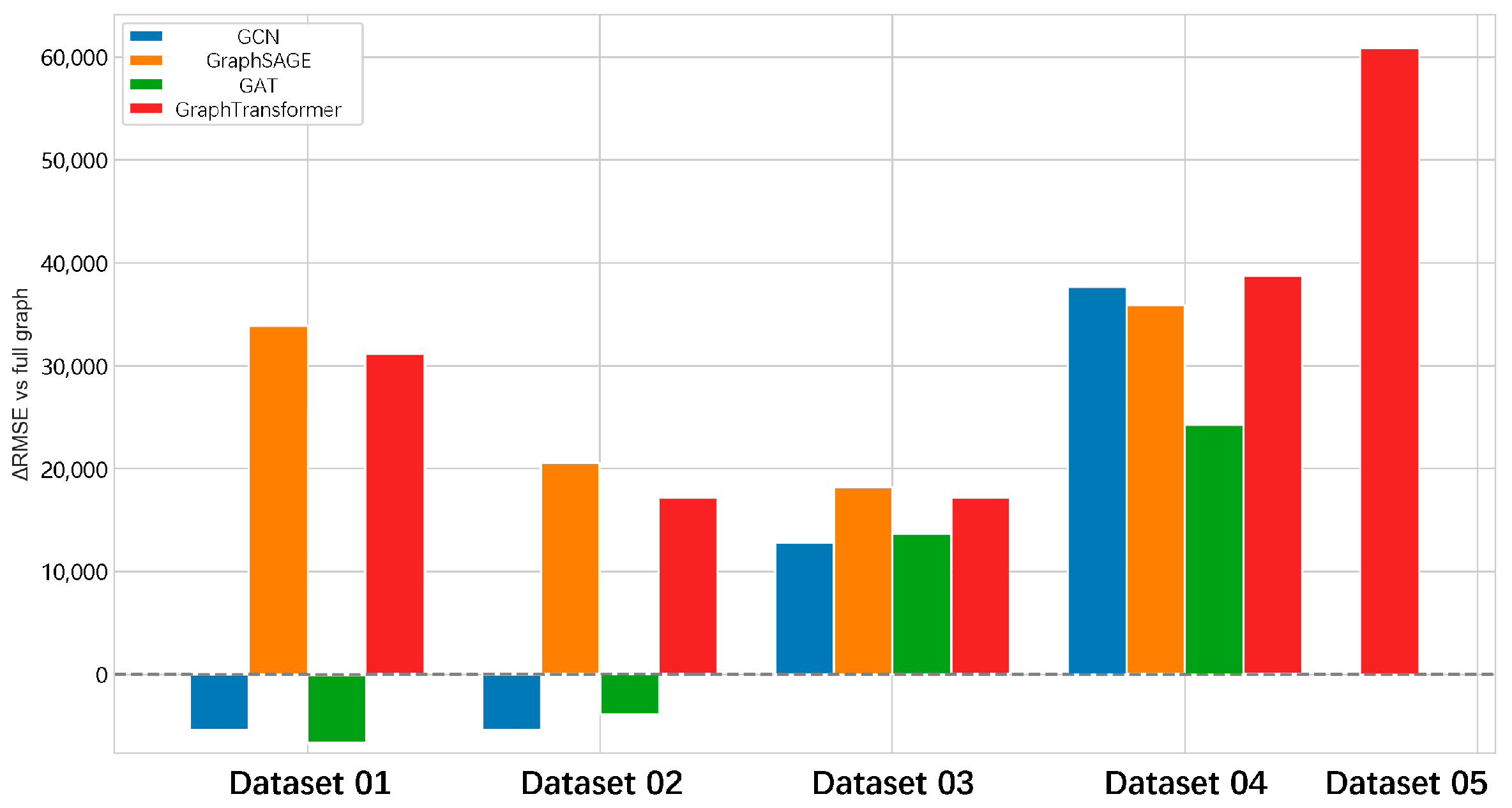
To evaluate the structural and feature dependencies of the GNN predictive models, four GNN algorithms were trained on five independent ablation datasets, and their performance was comparatively analyzed against the optimized baseline models trained on the fully GNN datasets. Based on feature analysis by GNNExplainer, $BH$ and $Area$ were identified as the important features for $F_{Cooling}$, whereas $BH$ and $L/W$ are the primary features for $F_{Heating}$. Consequently, the feature-based ablation datasets were created: Dataset 03 was generated by removing Area for $F_{Cooling}$ and L/W for $F_{Heating}$, while Dataset 04 was created by removing $BH$ for both scenarios.

As shown in Figure 25, in terms of ${\mathrm{F}}_{\mathrm{C}\mathrm{o}\mathrm{o}\mathrm{l}\mathrm{i}\mathrm{n}\mathrm{g}}$, the results demonstrate that all GNN models heavily rely on key structural and feature components for intelligent building energy prediction. For graph structures, both GraphSAGE and GraphTransformer exhibit a high dependency on BLG graph, where removing the buildings layout topology (Dataset 01) causes a more severe performance degradation ($∆\mathrm{R}\mathrm{M}\mathrm{S}\mathrm{E}$) than losing BZG (Dataset 02), while GCN and GAT show negative anomalies that suggest full-graph connections may induce structural noise or over-smoothing in simpler architectures. The result confirmed that the building layout arrangements have a significant impact on ${\mathrm{F}}_{\mathrm{C}\mathrm{o}\mathrm{o}\mathrm{l}\mathrm{i}\mathrm{n}\mathrm{g}}$.

Figure 25. The ablation study for $F_{Cooling}$ GNN models.

Regarding node attributes, $\mathrm{B}\mathrm{H}$ (Dataset 04) emerges as the universally dominant predictor whose absence triggers a massive performance collapse across all models, whereas the secondary feature, $\mathrm{A}\mathrm{r}\mathrm{e}\mathrm{a}$ (Dataset 03), yields a more moderate impact.

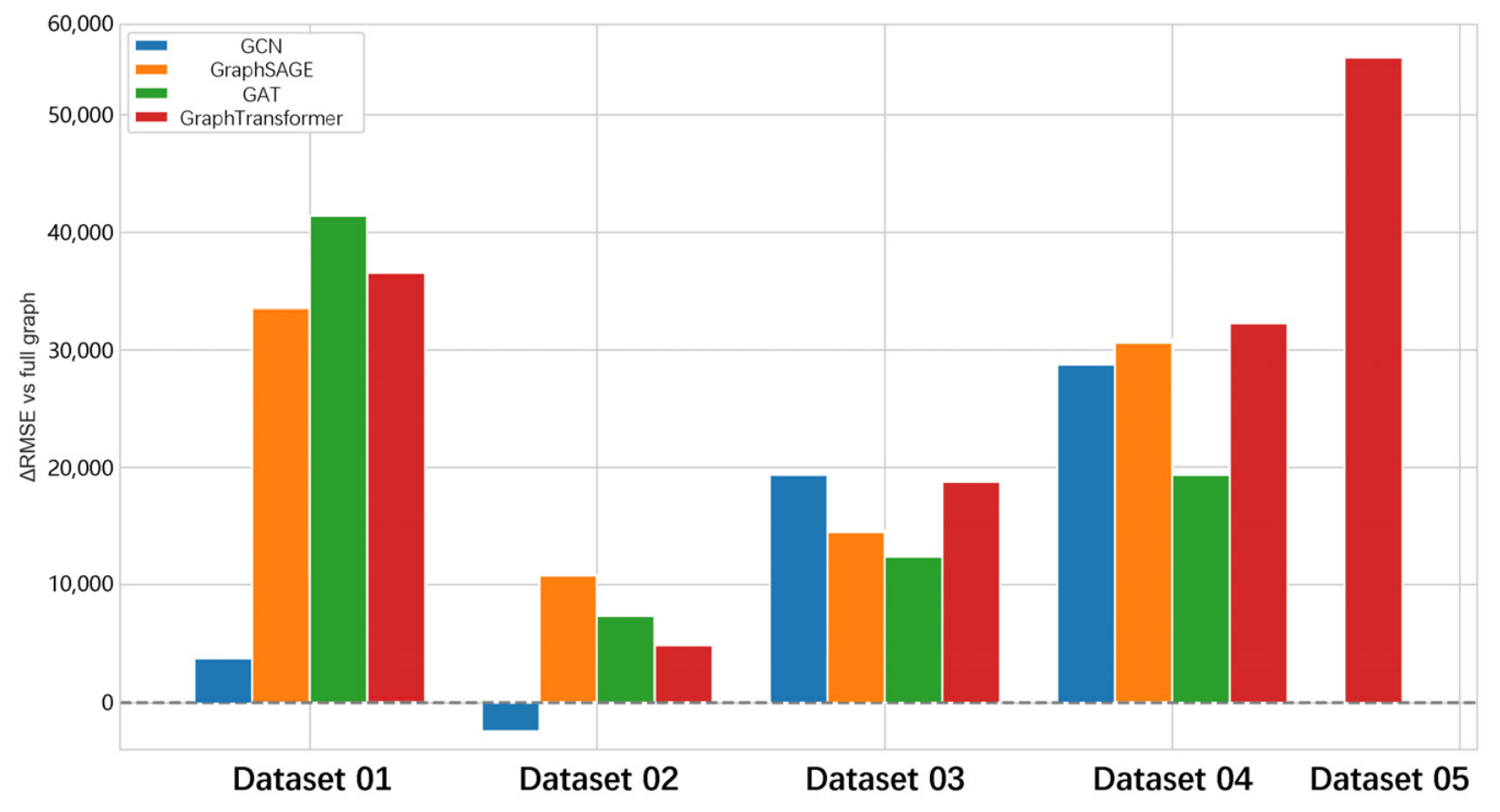
As shown in Figure 26, in terms of ${\mathrm{F}}_{Heating}$, the result demonstrates that all GNN models exhibit high sensitivity to specific topological structures, node features. Regarding graphs, removing the BLG topology (Dataset 01) has a significantly higher $∆\mathrm{R}\mathrm{M}\mathrm{S}\mathrm{E}$ than removing the BZG topology (Dataset 02) across nearly all models. This confirms that macro-level spatial arrangements exert a dominant influence on ${\mathrm{F}}_{Heating}$.

Figure 26. The ablation study for $F_{Heating}$ GNN models.

For node attributes, the higher error surge across all models is in Dataset 04, rather than in Dataset 03, thus validating $BH$ as a more critical predictor than $L/W$ for heating loads.

Finally, as shown in Figure 19 and Figure 20, the skip connection (Dataset 05) emerges as an absolute prerequisite for the architectural stability of the GraphTransformer, with its removal causing severe performance collapses in both $F_{Cooling}$ ($∆RMSE >\mathrm{60,000}$) and $F_{Heating}$ ($∆RMSE >\mathrm{50,000}$) predictions. This catastrophic degradation across both seasonal scenarios underscores that without skip connections, deep global attention layers inherently suffer from severe over-smoothing and representation washing.

4.5. The Efficiency and Accuracy Validation

As shown in Table 18, the GNN model achieved a 98.8% reduction in computational time compared to traditional EnergyPlus physics-based simulations. However, establishing such GNN surrogate models needs a large number of calculation results, which also need time during the initial data-generation phase. Consequently, the GNN framework offers a clear operational advantage in massive, multi-scenario block energy assessment tasks. On the other hand, the conventional EnergyPlus simulations still have advantages for low-volume computations.

Table 18. The calculation time of two methods.

Method	Number of Blocks	Total Calculation Time	Average Time
Energy-plus simulation	25	831 min	33 min 14 s
GNN prediction	25	575 s	23 s

As shown in Table 19, compared to recent State-of-the-Art urban energy models, both traditional machine learning and the GNN frameworks have excellent, comparable predictive fidelity, with $R^2$ values exceeding 0.85. Crucially, the GNN architecture significantly enhances data efficiency, using a dataset size representing a mere 7.3% of that required by Riccardo Taormi et al. [72] and 11.6% of that used by Ahad Montazeri et al. [73] This minimized data dependency shows the superior deployment scalability and broader practical prospects of the GNN-based framework.

Table 19. Performance comparison between different models.

Author and Year	The Method	City	Number of Samples	${\mathbf{R}}^{\mathbf{2}}$
Riccardo Talami et al. (2024) [72]	XGBoost	Tehran	3917	0.883 (monthly total)
Ahad Montazeri et al. (2025) [73]	LightGBM	Turin	2453	0.920 (thermal load)
The GNN Model	GraphTransformer	Wuhan	285	0.8560 (cooling)/0.9192 (heating)

5. Conclusions

Traditional surrogate models for urban building energy consumption often overlook spatial configurations and mutual shading effects, resulting in limited predictive accuracy. To address this, this study proposed a methodology based on GNNs. By using a heterogeneous graph approach, building morphology and layout information were successfully integrated by multilevel topological relationships. Based on heterogeneous graph data, node morphological features, and topological edge features from 265 blocks, four GNN models were developed. The optimal model was selected and validated using an independent set of 20 blocks. Finally, GNNExplainer was utilized to analyze critical features and message-passing mechanisms. The key conclusions are as follows:

• Model performance: GNN algorithms effectively predict both building cooling and heating energy consumption in a block. GraphTransformer achieved the best performance, with validation MSE values below 0.213 and 0.208, respectively. It demonstrated excellent generalizability on the validation dataset, with ${\mathrm{R}}^2$ values exceeding 0.85 for cooling and 0.90 for heating.
• Algorithm comparison: Due to the complex propagation patterns of urban data, GNN architecture exhibited significant performance differences. GraphSAGE and GraphTransformer outperformed others by effectively addressing the characteristic through sampling and global attention mechanisms, respectively.
• Error analysis: The prediction errors were most pronounced at the center nodes of the buildings. This is attributed to the complexity of processing heterogeneous information propagated from all surrounding nodes. Furthermore, as center nodes are entirely enclosed, GNNs find it hard to predict their energy demand solely from surrounding features without the indicators to distinguish them from peripheral nodes.
• The important features for $F_{Cooling}$: $Area$, $BH$, and $OZ$ are considered to be highly significant features in both optimal models. This shows the importance of footprint area, building shape factors, and facade orientation in cooling energy prediction. On the other hand, $D_x$ was critical for GraphTransformer, indicating that east–west building arrangements significantly influence cooling demand.
• The important features for $F_{Heating}$: Both optimal models mainly relied on $BH$ and $L/W$ for heating prediction, highlighting the significance of shape factor-related indicators. Like cooling, $D_x$ remained a key feature for GraphTransformer, emphasizing the impact of east–west spatial distribution on heating prediction.
• Signal propagation: GraphSAGE rarely utilized surrounding edge information, whereas the superior GraphTransformer consistently used signals from the west and south. This indicates that shading relationships from western and southern neighboring buildings are critical factors for accurate building energy prediction.

6. Limitations and Future Research

Although this study developed energy prediction models for Wuhan’s residential blocks with high accuracy and generalizability using heterogeneous graphs and various GNN algorithms―and identified key influential features via GNNExplainer―certain limitations remain to be addressed in future research:

• Simulation results’ validation: In this study, a GNN-based surrogate model was developed using simulated data. To bridge the discrepancies between simulated outputs and real building energy consumption, empirical validation is essential. Because field data collection needs temporal and coordination costs, future work will collaborate with the Power Supply Company in Wuhan to acquire large-scale consumption records for model training.
• Hierarchical message passing: Future work will change from a two-hop framework to a multilayer topology by defining urban blocks as macro-nodes. This path will implement multilevel attention mechanisms to simultaneously aggregate building morphological features and mesoscale climatic effects, thereby capturing cross-scale spatial dependencies to enhance prediction accuracy across expansive urban context.
• Comprehensive morphological indicators: The six morphological indicators used as node features do not fully capture architectural complexity. Future studies will incorporate a broader type of morphological indicator and use dimensionality reduction techniques such as Principal Component Analysis (PCA) to refine features for GNN training.
• Comprehensive dataset: The GNN dataset was generated from 285 blocks mainly located in Wuhan’s Jiang’an District, which may not represent the city’s entire residential diversity. On the other hand, the scale of dataset is limited, which makes the GNN model easy to overfit. Subsequent research will expand the dataset to include blocks from different administrative regions to ensure a more comprehensive urban-scale model.
• Integration of urban vegetation: The current model excludes the impact of block-level vegetation on energy consumption. Future research will use street-view and satellite imagery to digitize vegetation layouts for integration into the GNN framework.
• Physics-informed GNNs: To enhance model interpretability, future work will integrate thermodynamic constraints into the learning process, such as PhysGNN [74]. By incorporating physical loss functions, such as energy conservation and heat transfer equations, the model will ensure predictions adhere to physical laws, thereby improving generalization capabilities across diverse climatic scenarios.

References

1. Ribeiro, H.V.; Rybski, D.; Kropp, J.P. Effects of changing population or density on urban carbon dioxide emissions. Nat. Commun. 2019, 10, 3204. [Google Scholar] [CrossRef] [Scilit] [PubMed]
2. Zhang, Y.; Teoh, B.K.; Wu, M.; Chen, J.; Zhang, L. Data-driven estimation of building energy consumption and GHG emissions using explainable artificial intelligence. Energy 2023, 262, 125468. [Google Scholar] [CrossRef] [Scilit]
3. Shen, Y.; Pan, Y. BIM-supported automatic energy performance analysis for green building design using explainable machine learning and multi-objective optimization. Appl. Energy 2023, 333, 120575. [Google Scholar] [CrossRef] [Scilit]
4. Javanroodi, K.; Perera, A.T.D.; Hong, T.; Nik, V.M. Designing climate resilient energy systems in complex urban areas considering urban morphology: A technical review. Adv. Appl. Energy 2023, 12, 100155. [Google Scholar] [CrossRef] [Scilit]
5. Liu, X.; Tang, H.; Ding, Y.; Yan, D. Investigating the performance of machine learning models combined with different feature selection methods to estimate the energy consumption of buildings. Energy Build. 2022, 273, 112408. [Google Scholar] [CrossRef] [Scilit]
6. Mirzaei, P.A.; Haghighat, F. Pollution removal effectiveness of the pedestrian ventilation system. J. Wind Eng. Ind. Aerodyn. 2011, 99, 46–58. [Google Scholar] [CrossRef] [Scilit]
7. Lin, Y.; Yuan, X.; Yang, W.; Chan, M.; Tian, L. Impact of outdoor particulate matter 2.5 pollution on natural ventilation energy saving potential in office buildings in China. J. Build. Eng. 2023, 76, 107425. [Google Scholar] [CrossRef] [Scilit]
8. Fan, M.; Chau, C.K.; Chan, E.H.W.; Jia, J. A decision support tool for evaluating the air quality and wind comfort induced by different opening configurations for buildings in canyons. Sci. Total Environ. 2017, 574, 569–582. [Google Scholar] [CrossRef] [Scilit] [PubMed]
9. Li, Z.; Ma, J.; Jiang, F.; Zhang, S.; Tan, Y. Assessing the impacts of urban morphological factors on urban building energy modeling based on spatial proximity analysis and explainable machine learning. J. Build. Eng. 2024, 85, 108675. [Google Scholar] [CrossRef] [Scilit]
10. Cerezo Davila, C.; Reinhart, C.F.; Bemis, J.L. Modeling Boston: A workflow for the efficient generation and maintenance of urban building energy models from existing geospatial datasets. Energy 2016, 117, 237–250. [Google Scholar] [CrossRef] [Scilit]
11. Huang, W.; Xu, Q.; Zhao, B.; Lv, Q.; Wang, G. Urban multi-scale building energy modeling (BEM) and computational fluid dynamics (CFD) integration: Tools, strategies and accuracy for energy microclimate analysis. J. Build. Eng. 2025, 103, 112041. [Google Scholar] [CrossRef] [Scilit]
12. Henninger, R.H.; Witte, M.J.; Crawley, D.B. Analytical and comparative testing of EnergyPlus using IEA HVAC BESTEST E100–E200 test suite. Energy Build. 2004, 36, 855–863. [Google Scholar] [CrossRef] [Scilit]
13. Pasandi, L.; Qian, Z.; Woo, W.L. Quantifying urban microclimate feedback on building energy use using a coupled simulation workflow. Build. Environ. 2025, 285, 113657. [Google Scholar] [CrossRef] [Scilit]
14. Salvalai, G.; Zhu, Y.; Maria Sesana, M. From building energy modeling to urban building energy modeling: A review of recent research trend and simulation tools. Energy Build. 2024, 319, 114500. [Google Scholar] [CrossRef] [Scilit]
15. Reinhart, C.F.; Cerezo Davila, C. Urban building energy modeling—A review of a nascent field. Build. Environ. 2016, 97, 196–202. [Google Scholar] [CrossRef] [Scilit]
16. Ozturk, H.K.; Canyurt, O.E.; Hepbasli, A.; Utlu, Z. Residential-commercial energy input estimation based on genetic algorithm (GA) approaches: An application of Turkey. Energy Build. 2004, 36, 175–183. [Google Scholar] [CrossRef] [Scilit]
17. Zhang, Q. Residential energy consumption in China and its comparison with Japan, Canada, and USA. Energy Build. 2004, 36, 1217–1225. [Google Scholar] [CrossRef] [Scilit]
18. Howard, B.; Parshall, L.; Thompson, J.; Hammer, S.; Dickinson, J.; Modi, V. Spatial distribution of urban building energy consumption by end use. Energy Build. 2012, 45, 141–151. [Google Scholar] [CrossRef] [Scilit]
19. Ferrando, M.; Causone, F.; Hong, T.; Chen, Y. Urban building energy modeling (UBEM) tools: A state-of-the-art review of bottom-up physics-based approaches. Sustain. Cities Soc. 2020, 62, 102408. [Google Scholar] [CrossRef] [Scilit]
20. Lin, D.; Xu, X.; Liu, K.; Wu, T.; Wang, X.; Zhang, R. Interpretable data-driven urban building energy modeling considering inter-building effect. Build. Environ. 2025, 274, 112688. [Google Scholar] [CrossRef] [Scilit]
21. Li, W.; Zhou, Y.; Cetin, K.; Eom, J.; Wang, Y.; Chen, G.; Zhang, X. Modeling urban building energy use: A review of modeling approaches and procedures. Energy 2017, 141, 2445–2457. [Google Scholar] [CrossRef] [Scilit]
22. Zhao, H.; Magoulès, F. A review on the prediction of building energy consumption. Renew. Sustain. Energy Rev. 2012, 16, 3586–3592. [Google Scholar] [CrossRef] [Scilit]
23. Liu, K.; Xu, X.; Zhang, R.; Kong, L.; Wang, W.; Deng, W. Impact of urban form on building energy consumption and solar energy potential: A case study of residential blocks in Jianhu, China. Energy Build. 2023, 280, 112727. [Google Scholar] [CrossRef] [Scilit]
24. Reinhart, C.F.; Dogan, T.; Jakubiec, J.A.; Rakha, T.; Sang, A. Umi—An Urban Simulation Environment for Building Energy Use, Daylighting and Walkability. In Proceedings of the Building Simulation 2013: 13th Conference of IBPSA, Chambéry, France, 25–28 August 2013; pp. 476–483. [Google Scholar]
25. Zhang, R.; Xu, X.; Zhai, P.; Liu, K.; Kong, L.; Wang, W. Agile and integrated workflow proposal for optimising energy use, solar and wind energy potential, and structural stability of high-rise buildings in early design decisions. Energy Build. 2023, 300, 113692. [Google Scholar] [CrossRef] [Scilit]
26. Abbasabadi, N.; Ashayeri, M. Urban energy use modeling methods and tools: A review and an outlook. Build. Environ. 2019, 161, 106270. [Google Scholar] [CrossRef] [Scilit]
27. Ahmad, T.; Chen, H.; Guo, Y.; Wang, J. A comprehensive overview on the data driven and large scale based approaches for forecasting of building energy demand: A review. Energy Build. 2018, 165, 301–320. [Google Scholar] [CrossRef] [Scilit]
28. Pan, Y.; Zhu, M.; Lv, Y.; Yang, Y.; Liang, Y.; Yin, R.; Yang, Y.; Jia, X.; Wang, X.; Zeng, F.; et al. Building energy simulation and its application for building performance optimization: A review of methods, tools, and case studies. Adv. Appl. Energy 2023, 10, 100135. [Google Scholar] [CrossRef] [Scilit]
29. Norouziasl, S.; Jafari, A. Identifying the most influential parameters in predicting lighting energy consumption in office buildings using data-driven method. J. Build. Eng. 2023, 72, 106590. [Google Scholar] [CrossRef] [Scilit]
30. Lu, H.; Cheng, F.; Ma, X.; Hu, G. Short-term prediction of building energy consumption employing an improved extreme gradient boosting model: A case study of an intake tower. Energy 2020, 203, 117756. [Google Scholar] [CrossRef] [Scilit]
31. Fan, C.; Wang, J.; Gang, W.; Li, S. Assessment of deep recurrent neural network-based strategies for short-term building energy predictions. Appl. Energy 2019, 236, 700–710. [Google Scholar] [CrossRef] [Scilit]
32. Zhou, Y.; Tian, X.; Zhang, C.; Zhao, Y.; Li, T. Elastic weight consolidation-based adaptive neural networks for dynamic building energy load prediction modeling. Energy Build. 2022, 265, 112098. [Google Scholar] [CrossRef] [Scilit]
33. Pan, Y.; Zhang, L.; Yan, Z.; Lwin, M.O.; Skibniewski, M.J. Discovering optimal strategies for mitigating COVID-19 spread using machine learning: Experience from Asia. Sustain. Cities Soc. 2021, 75, 103254. [Google Scholar] [CrossRef] [Scilit]
34. Petch, J.; Di, S.; Nelson, W. Opening the Black Box: The Promise and Limitations of Explainable Machine Learning in Cardiology. Can. J. Cardiol. 2022, 38, 204–213. [Google Scholar] [CrossRef] [Scilit]
35. de Almeida, J.P.; Morley, J.G.; Dowman, I.J. A graph-based algorithm to define urban topology from unstructured geospatial data. Int. J. Geogr. Inf. Sci. 2013, 27, 1514–1529. [Google Scholar] [CrossRef] [Scilit]
36. Yan, X.; Ai, T.; Yang, M.; Yin, H. A graph convolutional neural network for classification of building patterns using spatial vector data. ISPRS J. Photogramm. Remote Sens. 2019, 150, 259–273. [Google Scholar] [CrossRef] [Scilit]
37. Yin, M.; Zhang, Z.; Wang, L.; Guo, X.; Qian, X.; Kamran, M. Optimizing Sustainable and Resilient Electric Vehicle Battery Recycling Network: Insights from Fourth-Party Logistics. Sustainability 2025, 17, 9872. [Google Scholar] [CrossRef] [Scilit]
38. Wu, Z.; Pan, S.; Chen, F.; Long, G.; Zhang, C.; Yu, P.S. A Comprehensive Survey on Graph Neural Networks. IEEE Trans. Neural Netw. Learn. Syst. 2021, 32, 4–24. [Google Scholar] [CrossRef] [Scilit] [PubMed]
39. Zhao, R.; Ai, T.; Yu, W.; He, Y.; Shen, Y. Recognition of building group patterns using graph convolutional network. Cartogr. Geogr. Inf. Sci. 2020, 47, 400–417. [Google Scholar] [CrossRef] [Scilit]
40. Li, Z.; Ma, J.; Wang, Q.; Wang, M.; Jiang, F. Enhancing urban solar irradiation prediction with shadow-attention graph neural networks: Implications for net-zero energy buildings in New York City. Sustain. Cities Soc. 2025, 120, 106133. [Google Scholar] [CrossRef] [Scilit]
41. Kim, J.; Yeom, S.; Ahn, S.; Seo, S.; Koo, C.; Hong, T. Operational day-ahead load forecasting using graph-based data-driven urban building energy modeling. Build. Environ. 2026, 294, 114384. [Google Scholar] [CrossRef] [Scilit]
42. Zhang, Y.; Liu, P.; Biljecki, F. Knowledge and topology: A two layer spatially dependent graph neural networks to identify urban functions with time-series street view image. ISPRS J. Photogramm. Remote Sens. 2023, 198, 153–168. [Google Scholar] [CrossRef] [Scilit]
43. Jia, Y.; Wang, J.; Hosseini, M.R.; Shou, W.; Wu, P.; Mao, C. Temporal graph attention network for building thermal load prediction. Energy Build. 2024, 321, 113507. [Google Scholar] [CrossRef] [Scilit]
44. Wu, Z.; Li, M.; Liu, W.; Cheng, J.C.P.; Wang, Z.; Kwok, H.H.L.; Huang, C.; Hou, F. Developing surrogate models for the early-stage design of residential blocks using graph neural networks. Build. Simul. 2025, 18, 679–698. [Google Scholar] [CrossRef] [Scilit]
45. Hu, Y.; Cheng, X.; Wang, S.; Chen, J.; Zhao, T.; Dai, E. Times series forecasting for urban building energy consumption based on graph convolutional network. Appl. Energy 2022, 307, 118231. [Google Scholar] [CrossRef] [Scilit]
46. Lu, J.; Zhang, C.; Li, J.; Zhao, Y.; Qiu, W.; Li, T.; Zhou, K.; He, J. Graph convolutional networks-based method for estimating design loads of complex buildings in the preliminary design stage. Appl. Energy 2022, 322, 119478. [Google Scholar] [CrossRef] [Scilit]
47. Liang, X.; Yap, W.; Biljecki, F. Heterogeneous graph neural networks for building attribute prediction from hierarchical urban features and cross-view imagery. ISPRS J. Photogramm. Remote Sens. 2026, 234, 185–204. [Google Scholar] [CrossRef] [Scilit]
48. Kipf, T.N.; Welling, M. Semi-Supervised Classification with Graph Convolutional Networks. arXiv 2016, arXiv:1609.02907. [Google Scholar] [CrossRef] [Scilit]
49. Devlin, J.; Chang, M.-W.; Lee, K.; Toutanova, K. BERT: Pre-training of Deep Bidirectional Transformers for Language Understanding. In Proceedings of the 2019 Conference of the North American Chapter of the Association for Computational Linguistics: Human Language Technologies, Minneapolis, MN, USA, 2–7 June 2019; pp. 4171–4186. [Google Scholar]
50. Vaswani, A.; Shazeer, N.; Parmar, N.; Uszkoreit, J.; Jones, L.; Gomez, A.N.; Kaiser, Ł.; Polosukhin, I. Attention is all you need. In Proceedings of the 31st Conference on Neural Information Processing Systems (NeurIPS 2017), Long Beach, CA, USA, 4–9 December 2017. [Google Scholar]
51. Yuan, H.; Yu, H.; Gui, S.; Ji, S. Explainability in graph neural networks: A taxonomic survey. IEEE Trans. Pattern Anal. Mach. Intell. 2022, 45, 5782–5799. [Google Scholar] [CrossRef] [Scilit]
52. Yan, X.; Huang, Z.; Ren, S.; Zhu, Q.; Yin, G.; Qi, J.; Bao, Y. Explainable urban renewal prediction at building-scale using hierarchical graph neural networks. ISPRS J. Photogramm. Remote Sens. 2026, 233, 609–622. [Google Scholar] [CrossRef] [Scilit]
53. Batty, M. Cities as Complex Systems: Scaling, Interaction, Networks, Dynamics and Urban Morphologies. In Encyclopedia of Complexity and Systems Science; Meyers, R.A., Ed.; Springer: New York, NY, USA, 2009; pp. 1041–1071. [Google Scholar]
54. Kong, B.; Ai, T.; Zou, X.; Yan, X.; Yang, M. A graph-based neural network approach to integrate multi-source data for urban building function classification. Comput. Environ. Urban Syst. 2024, 110, 102094. [Google Scholar] [CrossRef] [Scilit]
55. Lei, B.; Liu, P.; Milojevic-Dupont, N.; Biljecki, F. Predicting building characteristics at urban scale using graph neural networks and street-level context. Comput. Environ. Urban Syst. 2024, 111, 102129. [Google Scholar] [CrossRef] [Scilit]
56. Xia, B.; Li, Z. Optimization of residential urban-block morphology based on its synthetic effects on indoor and outdoor natural lighting environments. Sustain. Cities Soc. 2023, 97, 104698. [Google Scholar] [CrossRef] [Scilit]
57. Natanian, J.; Wortmann, T. Simplified evaluation metrics for generative energy-driven urban design: A morphological study of residential blocks in Tel Aviv. Energy Build. 2021, 240, 110916. [Google Scholar] [CrossRef] [Scilit]
58. Liu, K.; Xu, X.; Huang, W.; Zhang, R.; Kong, L.; Wang, X. A multi-objective optimization framework for designing urban block forms considering daylight, energy consumption, and photovoltaic energy potential. Build. Environ. 2023, 242, 110585. [Google Scholar] [CrossRef] [Scilit]
59. Li, H.; Han, Y.; Wang, T.; Wang, Z.; Li, Y.; Shen, H. Evolution of urban morphological polycentricity and the thermal response in Wuhan from 2000 to 2020. Sustain. Cities Soc. 2024, 100, 105055. [Google Scholar] [CrossRef] [Scilit]
60. Johari, F.; Munkhammar, J.; Shadram, F.; Widén, J. Evaluation of simplified building energy models for urban-scale energy analysis of buildings. Build. Environ. 2022, 211, 108684. [Google Scholar] [CrossRef] [Scilit]
61. Crawley, D.B.; Lawrie, L.K.; Winkelmann, F.C.; Buhl, W.F.; Huang, Y.J.; Pedersen, C.O.; Strand, R.K.; Liesen, R.J.; Fisher, D.E.; Witte, M.J.; et al. EnergyPlus: Creating a New-Generation Building Energy Simulation Program. Energy Build. 2001, 33, 319–331. [Google Scholar] [CrossRef] [Scilit]
62. Mosteiro-Romero, M.; Maiullari, D.; Pijpers-van Esch, M.; Schlueter, A. An Integrated Microclimate-Energy Demand Simulation Method for the Assessment of Urban Districts. Front. Built Environ. 2020, 6, 553946. [Google Scholar] [CrossRef] [Scilit]
63. Sadeghipour Roudsari, M.; Pak, M. Ladybug: A parametric environmental plugin for grasshopper to help designers create an environmentally-conscious design. In Proceedings of the Building Simulation 2013: 13th Conference of IBPSA, Chambéry, France, 25–28 August 2013; pp. 3128–3135. [Google Scholar]
64. Guo, X.; Wang, S.; Li, J. GAN-MIGA-Driven Building Energy Prediction and Block Layout Optimization: A Case Study in Lanzhou, China. Urban Sci. 2026, 10, 77. [Google Scholar]
65. Mirzabeigi, S.; Razkenari, M. Design optimization of urban typologies: A framework for evaluating building energy performance and outdoor thermal comfort. Sustain. Cities Soc. 2022, 76, 103515. [Google Scholar] [CrossRef] [Scilit]
66. ANSI/ASHRAE/IES Standard 90.1-2013 (2015 Supplement); Energy Standard for Buildings Except Low-Rise Residential Buildings. ASHRAE: Atlanta, GA, USA, 2015.
67. Akiba, T.; Sano, S.; Yanase, T.; Ohta, T.; Koyama, M. Optuna: A next-generation hyperparameter optimization framework. In Proceedings of the 25th ACM SIGKDD International Conference on Knowledge Discovery & Data Mining, Anchorage, AK, USA, 4–8 August 2019; pp. 2623–2631. [Google Scholar]
68. Chen, D.; Lin, Y.; Li, W.; Li, P.; Zhou, J.; Sun, X. Measuring and relieving the over-smoothing problem for graph neural networks from the topological view. Proc. AAAI Conf. Artif. Intell. 2020, 34, 3438–3445. [Google Scholar] [CrossRef] [Scilit]
69. Chen, Z.; Deng, Q.; Ren, H.; Zhao, Z.; Peng, T.; Yang, C.; Gui, W. A new energy consumption prediction method for chillers based on GraphSAGE by combining empirical knowledge and operating data. Appl. Energy 2022, 310, 118410. [Google Scholar] [CrossRef] [Scilit]
70. Li, H.; Wang, M.; Ma, T.; Liu, S.; Zhang, Z.; Chen, P.-Y. What improves the generalization of graph transformers? A theoretical dive into the self-attention and positional encoding. arXiv 2024, arXiv:2406.01977. [Google Scholar] [CrossRef] [Scilit]
71. Shin, M.; Haberl, J.S. A procedure for automating thermal zoning for building energy simulation. J. Build. Eng. 2022, 46, 103780. [Google Scholar] [CrossRef] [Scilit]
72. Eshraghi, P.; Dehnavi, A.N.; Mirdamadi, M.; Talami, R.; Zomorodian, Z.S. An AI-driven framework for rapid and localized optimization of urban open spaces. Smart Sustain. Built Environ. 2025, 1–27. [Google Scholar] [CrossRef] [Scilit]
73. Montazeri, A.; Zhou, X.; Mutani, G. Advancing Urban Building Energy Modeling: The Role of Hybrid Energy Modeling in Enhancing Energy Consumption Predictions. Chall. Sustain. 2025, 13, 525–534. [Google Scholar]
74. Salehi, Y.; Giannacopoulos, D. PhysGNN: A Physics-Driven Graph Neural Network Based Model for Predicting Soft Tissue Deformation in Image-Guided Neurosurgery. In Proceedings of the 36th Conference on Neural Information Processing Systems (NeurIPS 2022), New Orleans, LA, USA, 28 November–9 December 2022; Volume 35, pp. 37282–37296. [Google Scholar]
Disclaimer/Publisher’s Note: The statements, opinions and data contained in all publications are solely those of the individual author(s) and contributor(s) and not of MDPI and/or the editor(s). MDPI and/or the editor(s) disclaim responsibility for any injury to people or property resulting from any ideas, methods, instructions or products referred to in the content.
Article Metrics
Citations
Article Access Statistics
Multiple requests from the same IP address are counted as one view.