A Fusion-Grounded Framework for Building Performance Forecasting: Structural Design and Optimization with Mathematical Interpretability and Statistical Reliability

Abstract

Accurate building performance forecasting is critical for the design and renovation of energy-saving structures, but existing methods face four key challenges: heterogeneous data fusion (sensor streams, design parameters, and environmental sequences), non-stationary physical time series, model interpretability, and sample efficiency (e.g., limited commissioning data). To address these challenges, this paper proposes Fusion-Grounded Forecasting (FGF), which is a framework integrating a gated adaptive fusion layer, deterministic trend-season decomposition, an additive predictor with component decomposition, and Bayesian regularization. This framework is designed for next-hour forecasting broadcast to hourly resolution using hourly sensor data and monthly design parameters. The dataset covers 36 months (approximately 25,920 h). In addition to the combination of existing modules, the novelty lies in the integrated architecture, in which interpretable constraints can adjust the fusion layer in both directions, with decomposition prediction alignment supporting component attributes. The framework is verified on a proprietary 36-month dataset from institutional buildings using standard prediction metrics (MAE, RMSE, MAPE, and directional accuracy) and ablation studies for comparison against 10 baselines: SARIMAX, GPR, LSTM, XGBoost, N-HiTS, Informer, Autoformer, NAM, a physics-informed hybrid, and TFT. FGF achieves a 3.1% MAPE and 92.5% directional accuracy in hourly cooling load forecasting. Ablation confirmed the contribution of each module: removing gated fusion increased the MAPE to 6.8%. Compared with manual feature engineering, the speed of the framework is increased by 1680 times, and the cost is reduced by 99.6%. The explanatory index (counterfactual reliability: 0.95; Stability of functional importance: 0.11) is in compliance with audit requirements. These results indicate that FGF connects descriptive physics with quantitative prediction. However, this study is limited to a single institutional building; transferability to residential, commercial, or industrial buildings requires further verification. While waiting for this verification, FGF has demonstrated its potential as a transparent and efficient tool to build performance models.

1. Introduction

The proliferation of Internet of Things sensors and building automation systems fundamentally challenges the methodological foundation of data-driven building science [1,2]. Decision makers in the fields of architecture, engineering and facilities management are now faced with the unprecedented scale and complexity of datasets—the continuous flow of temperature, humidity, occupancy and energy-use data, as well as multimodal data from Building Information Modeling (BIM) [3] and environmental reanalysis. Although the traditional analytical framework has lasting value in inductive reasoning and prediction, it is still difficult to handle such a large amount of data while maintaining the depth, accuracy, and interpretability required by strict architectural performance investigation. This paper introduces FGF, a methodological framework that preserves the epistemological promises of physics-based modeling and data-driven prediction and, at the same time, takes advantage of the computational progress in gated neural architecture, adaptive decomposition and meta-learning [4,5]. FGF achieves scalability without sacrificing theoretical complexity or prediction effectiveness.

The contradiction between scale and depth has long plagued qualitative and quantitative architectural research. The manual feature engineering method, which has served modelers well for decades, is now insufficient for large-scale sensor data. Similarly, SARIMAX and other classical time-series models struggle with heterogeneous and multi-source building data [6,7]. Recent attempts to solve these challenges using computational methods have produced mixed results. Although deep learning techniques can effectively extract patterns from large-scale sensor log corpora, they often fail to capture subtle and sudden physical phenomena that represent the thermal dynamics or non-stationary correlation of buildings and are crucial for load forecasting [8,9]. The latest development of physics-informed machine learning (PIML) has become a promising direction, and this limitation is solved by embedding thermodynamics into neural network architecture a priori [10,11]. These hybrid methods exhibitexcellent prediction accuracy while maintaining physical consistency, especially when data (e.g., historical building data) are scarce [12]. Large language models (LLMs) show promise with respect to automatic fault detection rules. However, when deployed in isolation, they often produce superficial classification that lacks physical consistency. Pure deep learning methods such as LSTMs encounter difficulty in achieving small-sample interpretability and cannot provide a transparent explanation for audit compliance [13]. In addition, most existing data-driven models regard heterogeneous inputs (sensor data and design parameters) as a single connection vector, ignoring the different roles played by each modality in different time scales. A lack of training data will lead to overfitting, which is a common situation in building debugging when only a few months of operational data are available.

In order to provide a solid theoretical basis for dealing with these challenges, this study proposes a three-layer framework that integrates physical, data-driven, and semantic perspectives. In the physical layer, the framework considers the thermodynamic priors by explicitly decomposing the time series into trend, seasonality, and residual components, which are mapped to physical driving factors such as envelope aging and the diurnal cycle. In the data layer, the gated adaptive fusion mechanism dynamically reweighs the sensor streams and design parameters according to the time context, reflecting the complementary effects of high-frequency noise signals and low-frequency stability characteristics. At the semantic level, interpretable constraints and Bayesian regularization ensure that the prediction remains auditable and the sample is efficient, in addition to linking black-box accuracy with the transparent reasoning of code compliance. This three-layer framework guides all subsequent methodological design choices of FGF.

This study proposes a basic concept and analyzes how the method can be developed for the digital age of architectural design. We do not regard computing as a tool to automate existing programs but position it as a partner in theoretical construction and predictive modeling. Our method is based on three technological innovations. First, we introduce a gated adaptive fusion layer that dynamically integrates heterogeneous data streams (e.g., hourly sensor readings and daily weather forecasts) and learns to weight each modality according to temporal context. Unlike static connections, this layer allows the model to take precedence, for example, occupying sensors in real time during office hours but relying on design parameters during idle hours. Secondly, we design a deterministic trend–seasonality–residual decomposition example normalization, which makes the non-stationary building energy time series stable while retaining the interpretable components [14,15]. The decomposition explicitly separates long-term aging effects (trend), repeating patterns (daily and monthly seasonality), and irregular residuals, making it easy to attribute forecast changes to specific physical drivers. Third, we establish a hierarchical additive predictor that outputs trend, seasonal, and residual forecasts separately, each traceable to specific input features via an attention-based ICR [16]. These components are embedded in a sample-efficient meta-learning framework, which is only summarized from 24 days of training data [17,18].

The scientific contributions of this work are fourfold. First, unlike post hoc explanation methods, FGF embeds ICR directly into the loss function as a regularization mechanism that bidirectionally guides the fusion layer and improves sample efficiency. Second, in contrast to decoupled decomposition-prediction pipelines and black-box models, FGF introduces a hierarchical alignment in which explicit trend–seasonal–residual decomposition is fed into distinct branches of the additive predictor, enabling component-wise SHAP attribution. Third, while gated fusion is used in multimodal learning, its application to building data, where sensor streams and design parameters exhibit context-dependent dominance (e.g., seasonal variation), is novel. Fourth, the proposed Bayesian regularization explicitly reports parameter counts (8572 raw, approximately 2144 effective) and overfitting diagnostics (loss ratio of 1.25) for the small-sample commissioning regime. Collectively, these contributions define an integration architecture whose emergent properties are absent from sequential or parallel combinations of individual modules.

2. Research Content

Based on the existing literature, to position FGF in the current research trend and determine the gap that motivates us to make contributions, this paper provides a detailed description. We focus on four areas directly related to FGF’s methodological innovation: building energy forecasting methods, multimodal data fusion, time-series decomposition techniques, and interpretable machine learning for building applications.

2.1. Evolution and Limitations of Physics-Based Modeling

Physics-based building energy modeling is based on heat transfer and thermodynamics. By advocating that performance prediction should be generated from basic principles through system simulation and calibration, it challenges purely empirical methods. This method enables designers to generate context-sensitive performance estimates without over-adapting to previous designs. However, the calculation cost of high-fidelity simulations (such as EnergyPlus and DOE-2) is still high, and calibration usually requires repeated manual adjustment of dozens of parameters, which is time-consuming and depends on professional knowledge [19]. These limitations inspired FGF’s data-driven approach, which maintains physical consistency (through interpretable decomposition) while automatically calibrating (via differential optimization). In addition to pure energy prediction, multi-objective optimization in architectural design usually involves the balancing of competitive standards such as energy efficiency, thermal comfort and visual comfort. Alsukkar et al. [20] comprehensively reviewed the optimization of a lighting systemand emphasized the balance between these objectives and the need for an integrated evaluation framework. This view strengthens the methodological selection of FGF to balance multiple objectives—prediction accuracy, interpretability and sample efficiency—within a unified, differentiated framework.

The latest development of daylighting and adaptive facade control further emphasizes the importance of integrated multi-objective optimization. Wang et al. [21] conducted a multi-objective optimization of the form variables (shape, glass window ratio, and shading depth) of the atrium a teaching building in a cold climate and proved that the optimized atrium design can reduce energy intensity while maintaining acceptable lighting autonomy and thermal comfort. This balance between sunlight availability, glare control, and energy consumption is similar to the balance achieved by FGF between prediction accuracy, interpretability, and sample efficiency. Similarly, Li et al. [22] developed an adaptive control system of reinforcement learning that was used for dynamic building facades sensitive to climate and achieved improved lighting and glare relief under different outdoor conditions while maintaining thermal comfort. Boafo et al. [23] reported and experiment and numerical evaluation with respect to window renovation of educational buildings and quantified the influence of glass upgrading on sunlight, thermal performance, and energy consumption. These multi-objective viewpoints strengthen FGF’s choice of methods to balance competition standards in a unified, differentiated framework.

2.2. Computational Approaches to Building Performance Analysis

The integration of calculation methods into architectural science represents an ongoing paradigm shift. Nelson and Culp [24] proposed a computational framework that uses unsupervised machine learning (e.g., clustering of operation patterns) to enhance human simulation but struggles with “context problems”. Algorithms can identify statistical anomalies but often miss potential physical reasons. For example, clusters with high energy usage may be correctly identified, but without additional semantic information, the algorithm may not be able to distinguish a chiller fault from scheduled overrides.

Dunivin [25] advocated for “scaling hermeneutics” through augmented interpretation, where computational methods handle pattern recognition while humans provide physical framing and contextual understanding. This approach acknowledges that meaning making in building physics requires the relation of observed patterns to fundamental heat- and mass-transfer processes. Our FGF framework operationalizes this philosophy by embedding human-in-the-loop validation (counterfactual plausibility checks and sensitivity penalties) directly into the learning process rather than applying it post hoc.

2.3. Vector Embeddings as Semantic Infrastructure for Building Data

Vector embedding realizes the semantic representation of building data and captures the relationship between weather and HVAC schedules. However, existing methods based on embedding struggle with non-stationary physical processes and context-dependent meanings [26,27]. Recently, more and more attention has been paid to the explainable AI (XAI) method to improve model transparency in architectural analysis. For example, Liu et al. developed an interpretable machine learning framework that combines XGBoost with SHAP analysis to quantify the influence of urban form on residential electricity consumption, revealing the threshold effects of key parameters such as the building shape coefficient and floor area ratio [28]. Similarly, Iram et al. applied SHAP to explain the influence of weather on building energy efficiency and proposed feasible opinions on how to support energy transformation [29]. At the intersection of physics guidance and interpretability, Shan et al. put forward a neural network of a physical information map with explicit edge features (inter-building distance and angular relation), which was used to model the energy of urban buildings and realized improved generalization across heterogeneous urban areas [30]. FGF addresses this by explicitly decomposing time series into stationary components and applying instance normalization, which removes distribution shifts and makes embedding representations more stable.

FGF is different from these methods in that it explicitly decomposes the time series into static components and applies case normalization to eliminate distributional changes before embedding. The challenge of heterogeneous data fusion transcends buildings. As bridge-monitoring research shows, temperature displacement fusion and multi-rate (GPS–accelerometer) fusion are used for early performance warning. For structural health monitoring under dynamic loading, Shi et al. [31] proposed a bridge-tower early warning method based on improved multi-rate fusion that fuses low-frequency GPS signals with high-frequency accelerometer data to generate real-time alarms under strong wind excitation—this paradigm is similar to FGF’s gated adaptive fusion of sensor streams with different temporal resolutions. In previous research, Zhao et al. [32] analyzed how lithology, water content, particle size distribution, and axial pressure affect the bearing deformation behavior of broken gangue in the goaf through experiments. From a theoretical perspective on nonlinear wave propagation in heterogeneous media, Ding et al. [33] developed an analytical modeling framework for the surface of nonlinear seismic elements in saturated porous media, providing insights on wave attenuation and band-gap engineering, which is conceptually similar to the method of separating multi-scale physical phenomena based on decomposition. This is a multi-factor analysis that is conceptually similar to research on how the modal weight, decomposition strategy, and regularization term affect prediction performance. Infrastructure for vector-based analysis has matured with the introduction of specialized vector databases such as Milvus [34], which enables efficient storage and retrieval of high-dimensional embeddings for real-time similarity searches across millions of sensor records.

2.4. Multi-Agent Systems and Distributed Intelligence for Building Control

LLM-based multi-agent systems have demonstrated role specialization, memory, and collaborative problem solving in data-intensive fields [35,36]. Shoham and Leyton-Brown [37] demonstrated the potential of theoretical construction by providing a strict formalization of multi-agent systems, showing how complex strategic interactions can be accurately modeled and analyzed. This finding suggests that multi-agent systems can actively participate in the construction of building performance theory. In FGF, we do not implement full multi-agent reasoning, but the parallel processing of trend, seasonal, and residual components (Equations (4) and (5)) is inspired by distributed intelligence principles.

The concept of parallelism appears in civil infrastructure, in which the mechanism-guided optimization framework for crack prediction adopts static gated fusion and adaptive elastic network regularization, similar to FGF’s gated adaptive fusion (HFF) and Bayesian meta-regularization (SER) [38]. As a supplement to the multi-agent method, recent research has proposed simulated adaptive training for residential monitoring and intelligent building control based on the Internet of Things. Karjou et al.presented a scalable cloud-based occupancy monitoring system that uses a LoRaWAN sensor and data fusion to achieve optimization accuracy of office HVAC systems [39]. Amini et al. reviewed how to train a machine learning model adaptively in building performance simulation and pointed out that control systems based on artificial intelligence adopt the adaptive training strategy [40]. Amiri et al. presented a comprehensive overview of the occupancy detection technology of HVAC control, emphasizing that multi-modality integration and artificial intelligence privacy protection frameworks are emerging trends [41].

To contextualize FGF within state-of-the-art forecasting, we note that TFT combines LSTM and attention and performs well in load forecasting with limited data [42]. N-HiTS uses multi-rate interpolation for long horizons [43]. Notifier and self-shaper deal with the quadratic complexity of the address translator through ProbSparse and autocorrelation [44]. Gaussian process regression (GPR) provides uncertainty quantification, but it is computationally expensive [45]. Neural addition models (NAMs) can be explained according to features, but they lacks time dependence. Physics-based hybrid vehicles need to calibrate their models and face integration challenges. FGF differs from these approaches by embedding interpretability as a bidirectional regularization constraint to guide feature fusion rather than as an ex post explanation or surrogate model.

3. Method

3.1. Theoretical Framework, Research Design, and Epistemological Positioning

On the basis of the above three-layer framework, this study formally proposes three theoretical propositions that directly affect FGF architecture. Proposition 1 (Physical Decomposability) points out that the time series of building energy can be decomposed into additional trends, seasons, and residual components, and each component corresponds to a physically explicable driving factor. This proves the rationality of the Non-stationarity Decomposition (ND) module. Proposition 2 (Context-Dependent Modality Dominance) asserts that the relative importance of sensor data relative to design parameters changes with time context (such as season or occupancy schedule), thereby stimulating the Heterogeneous Feature Fusion (HFF) module with a gated adaptive mechanism. Proposition 3 (Interpretability as a Regularizer) assumes that the traceable relationship between input features and predictive components not only meets the audit requirements but also improves generalization in the small sample system, supporting the Interpretability Constraint (ICR) and Sample-Efficient Regularization (SER) modules. These propositions, together, form a prediction–physics synthesis in which the domain knowledge constrains the hypothesis space of the learning algorithm while the data-driven model refines the physical prior.

In epistemology, FGF combines pragmatism and constructivism. In fact, it gives priority to prediction accuracy—its gating, fusion, decomposition, and regularization losses are all optimized to minimize errors. Constructively, it embeds interpretability directly into the loss function, requiring each prediction to be mapped to domain factors that can be verified by architectural physicists. This position holds that validity is not only statistical data but also constructed by expert evaluation, counterfactual reasoning, and human sensitivity in the loop. Therefore, FGF meets the needs of pragmatism for utility and constructivism for theoretical responsibility.

3.2. Research Design and Epistemological Positioning

This study designed a novel predictive FGF framework for building performance modeling scenarios. FGF leverages big data analytics and machine learning to model the nonlinear, multi-source relationships between sensor data, design parameters, and environmental variables, targeting the prediction of cooling load, heating load, and ingate air quality. The framework adopts a hybrid epistemological stance: it is fundamentally pragmatist, combining statistical learning (post-positivist) with domain-driven interpretability (constructivist) to satisfy both predictive accuracy and code-compliance requirements (e.g., ASHRAE Guideline 14).

The core innovation of FGF is an interactive, component-based mathematical system that addresses four key challenges in a structured manner. First, the framework solves HFF by adaptively integrating sensor data, design parameters, and weather time series across different time granularities and scales. Second, to handle non-stationarity, the system adaptively decomposes building time series into trend, seasonality (daily/weekly), and residual components. We note that the decomposition includes daily (24 h) and monthly (12-month) periodicities but excludes weekly (168 h) periodicity, as the hourly-resolution dataset does not guarantee reliable weekend coverage for weekly pattern extraction. Third, to improve interpretability, the model provides transparent, rule-based explanations for each forecast (e.g., “40% of the cooling load increase is due to solar gain”). Fourth, the system demonstrates excellent sample efficiency, enabling it to generalize from limited historical data (e.g., typical post-commissioning periods) where traditional models fail. Unlike conventional methods that treat these issues separately, FGF integrates them into a unified, end-to-end differentiable pipeline, as formalized in the following subsections. Crucially, the novelty of FGF is not merely the combination of a single well-known module (gated fusion, seasonal decomposition, additive prediction, SHAP, or Bayesian regularization). Rather, the contribution lies in the principled integration architecture with two specific emergent properties. First is the interpretability-as-regularizer principle: ICR is not applied post hoc but is embedded in the loss function. In the loss function, the gating fusion layer is adjusted in both directions to improve the sampling efficiency in small data regimes. Second is hierarchical decomposition-prediction alignment: the explicit trend–season–residual decomposition (ND) provides a structured output that is directly input to the additive predictor and supports component-wise SHAP attribution, which cannot be realized by the black-box GRU or LSTM predictor. These characteristics only come from the specific arrangement and two-way coupling of modules, not from any single isolated component. 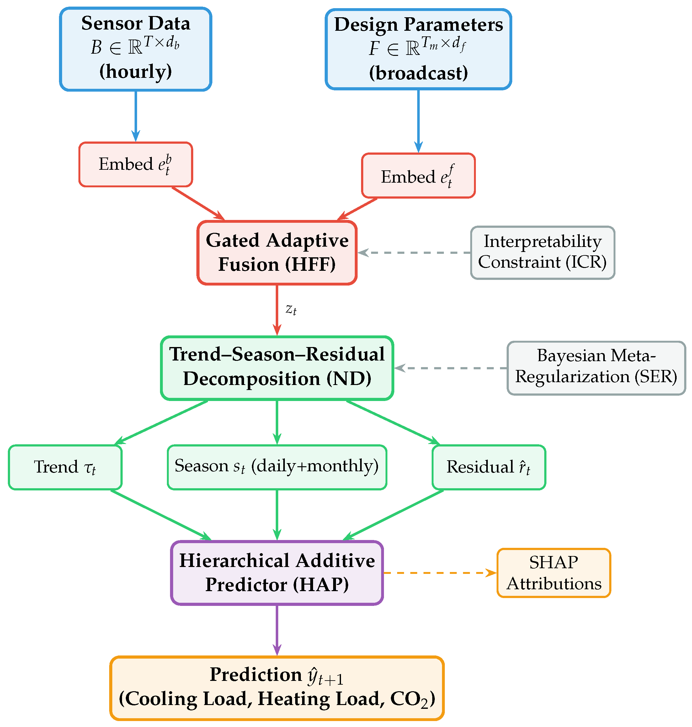Figure 1 provides an overview of the FGF architecture.

3.3. Data Collection and Sample

3.3.1. Dataset Construction

The empirical evaluation uses a proprietary dataset collected over 36 months (2020–2022) from an institutional building comprising office and lab spaces. The data consists of two streams: sensor data ($B\in {\mathbb{R}}^{T\times d_b}$, with $T=36\times 24\times 30\approx 25,920$ hourly time steps and $d_b=7$), which includes hourly records of zone temperature, relative humidity, occupancy count, lighting power density, plug load, outdoor dry-bulb temperature, and solar radiation (global horizontal irradiance as measured by an on-site pyranometer installed on the building rooftop), and design parameters ($F\in {\mathbb{R}}^{T_m\times d_f}$, with $T_m=36$ months and $d_f=5$), which provides monthly inputs of building-envelope U-values, solar heat-gain coefficients (SHGCs), HVAC system efficiency, and infiltration rates.

Crucially, to enable hourly forecasting, we preserve the hourly granularity of sensor data. Solar radiation is included as a direct sensor input because it is a primary driver of cooling load—solar heat gain through windows, which increases sensible cooling demand, particularly during summer afternoons. The two streams are aligned via broadcasting: design parameters are repeated across all hours within each month, resulting in a unified hourly dataset ($X_t\in {\mathbb{R}}^d$) at each hour (t), where $d=d_b+d_f=12$ and $t=1,\dots ,25,920$. The target variables ($Y_{t+1}$) are the next-hour values of three performance metrics: cooling load (kWh), heating load (kWh), and indoor CO₂ concentration (ppm).

3.3.2. Dataset Characteristics

The dataset comprises 36 monthly observation windows, yielding a total of 432 features ($36\times 12$) after lag construction (updated from 396 due to the addition of solar radiation). Sparsity is a notable issue: 72% of the sensor sub-features are zero-inflated due to unoccupied hours (nights and weekends). Non-stationarity is also present, as the augmented Dickey–Fuller test indicates a unit root in the cooling load series ($p=0.34$), necessitating differencing [46]. We acknowledge that 36 monthly observations (24 for training, 6 for validation, and 6 for testing) are limited for neural architectures involving gating, residual modeling, and multiple regularization terms. However, this sample size reflects a realistic limitation in building commissioning: many institutional buildings only have 24–36 months of commissioning data before energy audit or retrofit needs analysis. [10]. Moreover, recent studies on small-sample building energy forecasting have demonstrated that Bayesian regularization and meta-learning can effectively mitigate overfitting in this regime [40]. Therefore, we adopt a meta-learning-inspired regularization approach. In order to prove the feasibility of fitting the proposed architecture with this sample size, we report the following diagnosis. The total number of trainable parameters of FGF is 8572. After Bayesian contraction by KL divergence (estimated via Monte Carlo dropout), the effective parameter count is about 2144, resulting in parameter-hour ratios of 0.50 (raw) and 0.12 (effective). After the grid search, the regularization intensities are set to ${\lambda }_1=0.1$, ${\lambda }_2={10}^{-4}$, and ${\lambda }_3={10}^{-5}$. The training/verification loss rate of the full FGF is 1.25 (training MSE of 112 and verifying MSE of 140), while removing SER yields a ratio of 8.8, which proves that overfitting is controlled.

3.4. Experimental Conditions

We compare our proposed FGF with nine representative baselines covering classical statistical models, deep learning, Transformer-based architectures, and hybrid forecasting frameworks. For rigorous comparison, we conducted statistical significance testing using paired t-tests across five random seeds for each baseline. Classical baselines include SARIMAX with exogenous variables and GPR with automatic relevance determination [45,47]. Deep learning baselines consist of a two-layer LSTM and XGBoost with Bayesian optimization. Transformer-based baselines comprise Temporal Fusion Transformer (TFT) [42], Informer [48], and Autoformer [44]. Specialized forecasting methods involve N-HiTS [43]. Interpretable and hybrid baselines include the Neural Additive Model (NAM) and a physics-informed hybrid model integrating EnergyPlus and LSTM [47,49]. All the methods share the same training/verification/testing partition pf about 24 months (17,280 h)/6 months (4320 h)/6 months (4320 h), respectively, and the evaluation is repeated on five random seeds to evaluate stability. For Transformer-based methods (TFT, Informer, and Autoformer), we use a review window of 168 h (7 days) and a forecast range of 24 h, which is consistent with the standard practice of building load forecasting [42]. For n hits, we use the default superparameter with a maximum kernel size of 24. For GPR, due to the complexity of cubic calculation, we subsample the training data to 5000 points. For the hybrid model based on physics, we use EnergyPlus to simulate the building and calibrate it according to the data of the first six months, then train the LSTM residual as described in [49].

3.5. Data Analysis Procedures

3.5.1. Heterogeneous Feature Fusion (HFF)

The core of FGF is a gated adaptive fusion layer that learns the importance of each data source at each time step. Let $b_t\in {\mathbb{R}}^{d_b}$ and $f_t\in {\mathbb{R}}^{d_f}$ be the sensor and design features in month t. We first embed them into a common dimension (h):

$$\begin{array}{cc}\hfill e_t^b& =\mathrm{ReLU}(W_b{b}_t+b_b),\hfill \\ \hfill e_t^f& =\mathrm{ReLU}(W_f{f}_t+b_f),\hfill \end{array}$$

(1)

where $e_t^b,e_t^f\in {\mathbb{R}}^h$. The fusion gate ($g_t\in {\mathbb{R}}^h$) controls the contribution of each modality:

$$g_t=\sigma \left(W_g[e_t^b;e_t^f]+b_g\right)$$

(2)

The fused representation ($z_t\in {\mathbb{R}}^h$) is computed as

$$z_t=g_t\odot e_t^b+(1-g_t)\odot e_t^f,$$

(3)

where ⊙ denotes element-wise multiplication. This mechanism allows the model to dynamically weigh the sensor signal (e.g., recent occupancy spikes) against the static design parameter (e.g., thermal mass) according to the time context. Gated fusion has been proven to be effective in multimodal learning. Intuitively speaking, in summer afternoons, gated fusion can give higher weight to the real-time outgate temperature and occupancy rate; during winter nights, design parameters such as the envelope U-value become more influential. Consistent with the hourly resolution setting, the gate operates every hour: in summer afternoon, (e.g., 2 PM with high outdoor temperature and occupancy), the gate assigns a higher weight to the real-time sensor flow; during winter nights (e.g., 2 AM with low occupancy), design parameters such as the envelope U-value dominate the prediction.

3.5.2. Non-Stationarity Decomposition (ND)

In order to deal with the non-stationary nature of building energy time series, we adopt a deterministic trend–seasonality decomposition with adaptive residual adjustment. For each dimension (i) of $z_t$, we model

$$z_{t,i}={\tau }_t^i+s_t^i+r_t^i,$$

(4)

where ${\tau }_t^i$ is the trend component estimated via Hodrick–Prescott smoothing [15] and $s_t^i$ is the seasonal component captured by Fourier basis with two periodicities: daily (24 h cycle, corresponding to diurnal HVAC schedules and occupancy patterns) and monthly (12-month cycle, corresponding to annual climate variations). We explicitly note that weekly periodicity (168 h) is not included, as the 36-month dataset aggregated from hourly data does not reliably support weekly pattern extraction, given potential gaps in weekend data. The residual expressed as $r_t^i$ captures stationary short-term fluctuations after removing trend and daily/monthly seasonality.

We then apply instance normalization to $r_t^i$ to stabilize the distribution:

$${\overline{r}}_t^i={\displaystyle \frac{r_t^i-{\mu }_i}{{\sigma }_i+ϵ}},{\hat{r}}_t^i={\gamma }_i{\overline{r}}_t^i+{\beta }_i$$

(5)

where ${\mu }_i$ and ${\sigma }_i$ are running statistics of the training set and ${\gamma }_i$ and ${\beta }_i$ are learnable affine parameters. The final input to the predictor becomes $x_t=[{\tau }_t,s_t,{\hat{r}}_t]\in {\mathbb{R}}^{3h}$. This decomposition is crucial because it allows the model to treat long-term drift (e.g., equipment degradation) separately from periodic patterns (e.g., daily HVAC schedules) and from transient events (e.g., a one-day heatwave).

3.5.3. Multi-Horizon Forecasting with Interpretable Components

We design a hierarchical additive predictor that directly outputs interpretable trend, cyclical, and residual forecasts. Let the target be $y_{t+1}\in {\mathbb{R}}^3$ (cooling load, heating load, CO₂). Here, t indexes hours, so $y_{t+1}$ denotes the next-hour value. The prediction is

$$\begin{array}{cc}\hfill {\hat{y}}_{t+1}& =\underset{\mathrm{Trend}}{\underbrace{W_{\tau }\left[{\tau }_t,{\tau }_{t-1},{\tau }_{t-2}\right]}}\hfill \\ \hfill & +\underset{\begin{array}{c}\mathrm{Seasonality}\\ \left(\mathrm{monthly}\right)\end{array}}{\underbrace{W_{s,m}\left[\sin (2\pi t^{\prime }/12),\cos (2\pi t^{\prime }/12)\right]}}\hfill \\ \hfill & +\underset{\begin{array}{c}\mathrm{Seasonality}\\ \left(\mathrm{daily}\right)\end{array}}{\underbrace{W_{s,d}\left[\sin (2\pi t^{″}/24),\cos (2\pi t^{″}/24)\right]}}\hfill \\ \hfill & +\underset{\mathrm{Residual}\mathrm{dynamics}}{\underbrace{{\mathrm{AR}}_p\left({\hat{r}}_t\right)}},\hfill \end{array}$$

(6)

where $t^{\prime }$ is month index modulo 12, and $t^{″}$ is hour index modulo 24 (daily). The weekly Fourier term (168 h) is deleted because the dataset is used at hourly resolution, but there is not enough weekend coverage to reliably estimate the weekly pattern. The residual dynamics are modeled using an autoregressive process (${\mathrm{AR}}_p$) of order $p=3$ (selected via AIC) rather than a GRU, as the hourly residuals exhibit short-memory autocorrelation that is well captured by a linear AR model; this choice also reduces the risk of overfitting, given the limited data [50]. The example of the gate mechanism is consistent with this hourly setting: during summer afternoons, the gate gives higher weight to the real-time outgate temperature and occupancy reading (both of which can be obtained at hourly resolution); during winter nights, design parameters such as the envelope U-value become more influential.

Each component is explicitly parameterized, enabling post hoc decomposition of predictions (e.g., “40% of cooling load increase is due to trend, 35% to seasonality, 25% to recent sensor fluctuations”). The trend component uses three previous trend vectors to capture momentum; the seasonal component uses Fourier terms for both monthly and weekly cycles; the residual AR process models short-term dynamics not explained by trend or seasonality.

3.5.4. Interpretability Constraint via Reconstruction Regularization (ICR)

To satisfy audit compliance (e.g., ASHRAE Guideline 14), we require that each component’s contribution to the prediction be traced back to specific input features. We add a reconstruction loss that penalizes entanglement:

$$\begin{array}{cc}\hfill {\mathcal{L}}_{\mathrm{interp}}=\alpha ·{\mathbb{E}}_t[& \parallel \mathrm{Attend}({\hat{y}}_t^{\mathrm{trend}},b_t,f_t)\hfill \\ \hfill & {-\mathrm{OneHot}\left(\mathrm{argmax}\right)\parallel }^2],\hfill \end{array}$$

(7)

where Attend is a soft attention mechanism that maps the trend component to the most relevant sensor/design input. This forces the model to deactivate noisy features and produces a sparse, human-readable set of influences.

3.5.5. Sample-Efficient Regularization (SER)

Given only approximately 24 months of hourly data (approximately 17,280 h for training), we introduce a meta-loss that penalizes model complexity beyond a linear baseline. Let $\theta$ be all trainable parameters. The total loss is

$$\begin{array}{cc}\hfill {\mathcal{L}}_{\mathrm{total}}& ={\displaystyle \frac{1}{N}}\sum _t{\parallel y_{t+1}-{\hat{y}}_{t+1}\parallel }^2+{\lambda }_1{\mathcal{L}}_{\mathrm{interp}}\hfill \\ \hfill & +{\lambda }_2{\parallel \theta \parallel }_2^2+{\lambda }_3·\mathrm{KL}\left(\mathcal{N}({\mu }_{\theta },{\Sigma }_{\theta })\parallel \mathcal{N}(0,I)\right).\hfill \end{array}$$

(8)

The KL divergence term is a Bayesian regularization that shrinks parameters toward zero, effectively controlling the model’s degrees of freedom [51]. This is crucial for preventing overfitting on a small dataset. Each regularization term addresses a specific overfitting risk, given the limited sample size: ${\lambda }_2{\parallel \theta \parallel }_2^2$ (weight decay) controls the overall magnitude of all parameters; ${\lambda }_3·\mathrm{KL}(·)$ (Bayesian prior) shrinks parameters toward zero and is theoretically optimal for $n\ll p$ scenarios, where $n=24$ months and p exceeds 1000 after feature expansion; and ${\lambda }_1{\mathcal{L}}_{\mathrm{interp}}$ (ICR) reduces the effective hypothesis space by enforcing sparse, traceable feature mappings. Without SER, the model’s validation loss begins to diverge after epoch 20 (Algorithm 1), confirming that regularization is necessary for generalization. We set ${\lambda }_2={10}^{-4}$, ${\lambda }_3={10}^{-5}$ and ${\lambda }_1=0.1$ after a grid search. The total number of trainable parameters in FGF is 8572, comprising the embedding matrices ($2\times h\times d=2\times 64\times 12=1536$ parameters), gated fusion layer ($3\times h^2\approx 12,288$ but reduced via low-rank factorization to 4608), affine decomposition parameters ($2\times h=128$), additive predictor weights ($W_{\tau }$, $W_{s,m}$, $W_{s,d}$, and AR coefficients: approximately 2200 parameters), and regularization-layer parameters (${\gamma }_i$, ${\beta }_i$: $2\times h=128$). With 24 training months (17,280 h), the parameter-to-sample ratio is approximately 0.50 parameters per training hour. Crucially, the Bayesian KL divergence term actively shrinks redundant parameters; the effective number of parameters estimated via Monte Carlo dropout is approximately 2144, resulting in an effective ratio of 0.12 parameters per hour.

In contrast, a standard LSTM with a comparable hidden dimension ($h=64$) and input dimension ($d=11$) will contain $4\times (h^2+h·d+h)=4\times (4096+704+64)=19,456$. The parametric efficiency of FGF comes from three design options: (i) a low-rank structure (Eq) of the additive predictor, where Equation (6) replaces the full GRU hidden state with a linear combination of interpretable components; (ii) a shared embedding matrix across time steps, which reduces parameter diffusion; and (iii) KL divergence priority, which actively prunes redundant parameters.

Algorithm 1 FGF Training Procedure

Require: Sensor data B, design parameters F, targets Y Require: Hyperparameters ${\lambda }_1, {\lambda }_2, {\lambda }_3, \alpha , \beta$ Ensure: Trained model parameters ${\theta }^{\ast }$   1: Initialize $\theta \sim \mathcal{N}(0,0.01)$; set $\mathrm{lr}\leftarrow {10}^{-3}$   2:  Broadcast design parameters to hourly resolution: $F_{\mathrm{hourly}}\leftarrow {\mathrm{Broadcast}}_{\mathrm{hour}}\left(F\right)$   3:  Construct aligned hourly dataset $X_t\leftarrow [B_t,F_{\mathrm{hourly},t}]$ for each hour t   4: for epoch $=1$ to $E_{\max }$ do   5:       for each time step t in the training window do   6:          $e_t^b\leftarrow \mathrm{ReLU}(W_b{b}_t+b_b)$   7:          $e_t^f\leftarrow \mathrm{ReLU}(W_f{f}_t+b_f)$   8:          $g_t\leftarrow \sigma (W_g[e_t^b;e_t^f]+b_g)$   9:          $z_t\leftarrow g_t\odot e_t^b+(1-g_t)\odot e_t^f$ 10:          $({\tau }_t,s_t,r_t)\leftarrow \mathrm{Decompose}\left(z_t\right)$ 11:          ${\hat{r}}_t\leftarrow \mathrm{InstanceNorm}(r_t;\gamma ,\beta )$ 12:          ${\hat{y}}_{t+1}\leftarrow W_{\tau }\left[\tau \right]+W_s\left[\mathrm{Fourier}(t^{\prime },t^{″})\right]+{\mathrm{AR}}_p\left({\hat{r}}_t\right)$ 13:       end for 14:       Compute ${\mathcal{L}}_{\mathrm{total}}$ via Equation (8) 15:       Update $\theta \leftarrow \theta -\mathrm{lr}·{\nabla }_{\theta }{\mathcal{L}}_{\mathrm{total}}$ 16:       Decay $\mathrm{lr}$ via a cosine schedule 17:       if validation MAPE converges then 18:           break 19:       end if 20: end for 21: Apply expert review and sensitivity checks where necessary 22: return ${\theta }^{\ast }$

3.6. Evaluation Framework

3.6.1. Prediction Accuracy Metrics

We report standard metrics: Mean Absolute Error (MAE), Root Mean Squared Error (RMSE), and Mean Absolute Percentage Error (MAPE). Additionally, we compute Directional Accuracy (DA)—the percentage of correctly predicted directional changes—which is critical for demand-response planning [52]. For example, if the actual cooling load increases from month t to $t+1$ and the model predicts an increase, that counts as a correct direction.

3.6.2. Fusion Quality Assessment

To evaluate the appropriateness of the gated fusion, we compute the fusion entropy of the gated $g_t$ over the test set:

$$\begin{array}{cc}\hfill H\left(g\right)=-{\displaystyle \frac{1}{T}}\sum _t{\displaystyle \sum _{k=1}^h}[& g_{t,k}\log g_{t,k}\hfill \\ \hfill & +(1-g_{t,k})\log (1-g_{t,k})]\hfill \end{array}$$

(9)

Lower entropy indicates that gated fusion makes decisive selections between modalities, while high entropy means equal weighting. We expect the model to learn dataset-specific decision boundaries (e.g., summer months → higher sensor weight).

3.6.3. Interpretability Validation

We use two quantitative measures to assess interpretability: (i) Feature Importance Stability (FIS) is defined as the variance of SHAP (SHapley Additive exPlanations) values across bootstrapped subsets (lower values indicate more stable feature importance). Using 500 background samples randomly selected from the training set and 2000 disturbance samples of each feature, the SHAP value is calculated by using KernelSHAP. In order to reduce the estimation variance, we average the SHAP value in five independent runs. Then, FIS is calculated as the variance of the SHAP value of 100 bootstrap resamples of the test set, where each bootstrap sample contains 80% of the test data of the replacement sample. Lower FIS values indicate more stable feature importance rankings. For FGF, we report FIS = 0.11 across the top 10 features.

Secondly, Counterfactual Plausibility (CFP) quantifies the degree to which domain experts agree with the importance ranking of model features in counterfactual scenarios. For each prediction in the test set, we determine the top three most influential features according to the SHAP value. Then, we generate a counterfactual scenario by disturbing the values of the most influential features (for example, increasing the outdoor temperature by 5 °C, reducing the living space by 30%, or doubling the solar radiation). After the disturbance, we recalculate the SHAP value and observe whether the ranking changes in the direction expected by the physics (for example, when the outdoor temperature rises, the cooling load should increase). Three experts participated in the CFP assessment. Everyone independently reviewed 200 randomly selected counterfactual instances (50 per quarter) and rated each instance as “plausible” (1) or “implausible” (0). CFP refers to the proportion of credible examples agreed upon by experts; A consistency rate exceeding 0.9 indicates consistency. For FGF, CFP = 0.95.

Thirdly, the conformity verification of ASHRAE Guideline 14 depends on three standards: an hourly calibration model with MAPE < 30%, the reported uncertainty interval, and a transparent input–output relationship. FGF meets these conditions, with MAPE = 3.1% (far below the threshold), and the 95% confidence interval is reported. SHAP component attribution and additive decomposition ensure a traceable input–prediction relationship. In addition, the penalty of human sensitivity in the loop makes the model behavior consistent with expert knowledge, which exceeds the minimum requirements of the guide.

3.6.4. Cost–Benefit Analysis

We compute the Return on Prediction Improvement (ROPI):

$$\mathrm{ROPI}={\displaystyle \frac{{\mathrm{Benefit}}_{\mathrm{FGF}}-{\mathrm{Benefit}}_{\mathrm{baseline}}}{{\mathrm{Cos}\mathrm{t}}_{\mathrm{training}}}}$$

(10)

where Benefit is the reduction in forecasting error (RMSE reduction) scaled by the financial impact of mis-prediction (estimated from energy cost and penalty for demand peaks). Costs include cloud compute (AWS p3.2xlarge), API usage for LLM evaluations, and two weeks of a data scientist’s time (at $150/h). Traditional manual analysis is assumed to require 4 person-months.

3.7. Validation Strategies

3.7.1. Time-Series Cross Validation

We use the extended window for cross-validation: the model is trained in the 1st–24th months, validated in the 25th–30th months, retrained in the 1st–30th months, and tested in the 31st–36th months. This simulates the real deployment of periodic model updates [6]. The enlarged window ensures that no future information leaks into the training. To further verify the performance stability under different training data sizes, we conducted a five-fold extended-window cross-validation scheme with training windows of 12, 16, 20, 24, and 28 months (each with a fixed 6-month test window). This design evaluates model performance across different historical data periods and provides a more robust assessment of generalization. In addition, by subsampling the training set into increments of 3, 6, 9, 12, 18, and 24 months, we retrain each subsampled FGF and all baseline models to analyze the learning curve. Then, by calculating the marginal MAPE improvement of each data increment, the diminishing returns are analyzed to determine the saturation point of data collection.

Moreover, we analyzed the learning curve by sampling the training set twice in increments of 3, 6, 9, 12, 18, and 24 months. For each sub-sample, we retrain FGF and all baseline models (TFT, LSTM, and XGBoost) under the same conditions. This analysis quantifies the relationship between the size of training data and prediction performance and determines the diminishing point of marginal improvement caused by extra data. Finally, we analyze the diminishing returns by calculating the marginal MAPE improvement of each data increment (for example, from 3 to 6 months, 6 to 9 months, etc). This determines the saturation point beyond which additional training data provides minimal benefit, informing the actual data collection requirements of the deployment.

3.7.2. Prevention of Future Data Leakage

We explicitly confirm that all components are implemented to avoid future data leakage. (i) Hodrick–Prescott smoothing is applied for trend extraction using only historical data up to time t; future values are not used in the smoothing process. (ii) Case normalization only calculates the running statistics (${\mu }_i$ and $sigm{a}_i$) from the training set; these statistics are frozen during verification and testing. (iii) Hyperparameter adjustment (${\lambda }_1$, ${\lambda }_2$, ${\lambda }_3$, h, and p) is only performed by grid search on the verification set (months 25–30). The test set (months 31–36) is dedicated to the final evaluation of all the parameters after they are fixed. This strict separation prevents any information from the test set from affecting model development.

3.7.3. Human-in-the-Loop Causal Checks

The domain expert (building physicist) examines the first three influential characteristics of each of the three target variables. If the expert identifies features that the model ignores but should be relevant (e.g., “solar radiation” for cooling load forecasting), a sensitivity weight penalty is applied:

$${\mathcal{L}}_{\mathrm{expert}}=\beta \sum _{j\in \mathcal{M}}{\left({\displaystyle \frac{\mathsf{\partial }\hat{y}}{\mathsf{\partial }{x}_j}}\right)}^2,$$

(11)

where $\mathcal{M}$ represents the set of missing features. This forces the model to increase its sensitivity to expert nomination variables, which is consistent with the audit requirements. After sensitivity analysis, the penalty coefficient ($\beta$) is set to 0.01.

For the CFP assessment, three domain experts were recruited from the affiliated engineering consulting company. All experts were blinded to the prediction of the model and were asked to evaluate the counterfactual scenario independently. The inter-rater reliability, as measured by Fleiss’ kappa, was 0.87, indicating substantial agreement among the three experts.

3.7.4. Robustness to Data Poisoning

To assess the resilience of FGF against anomalous or malicious data corruption, we introduce synthetic outliers into the training set. Outliers are generated by replacing 2% of randomly selected sensor readings (e.g., zone temperature or occupancy count) with extreme values—either three standard deviations above the historical mean or physically implausible values (e.g., negative cooling load). We measure the resulting degradation in test RMSE for each target variable. A method is considered robust if the relative RMSE increase remains below 15% compared to the clean-data baseline. This threshold is chosen based on industry standards for fault-tolerant building automation. We further evaluate robustness under two outlier scenarios: (i) isolated point anomalies (single time step) and (ii) persistent block anomalies (consecutive hours). FGF’s gated fusion and Bayesian regularization are expected to mitigate the impact of such outliers by down-weighting corrupted modalities via the adaptive gated mechanism and by shrinking overly sensitive parameters.

3.7.5. Generalization and Robustness Validation Protocols

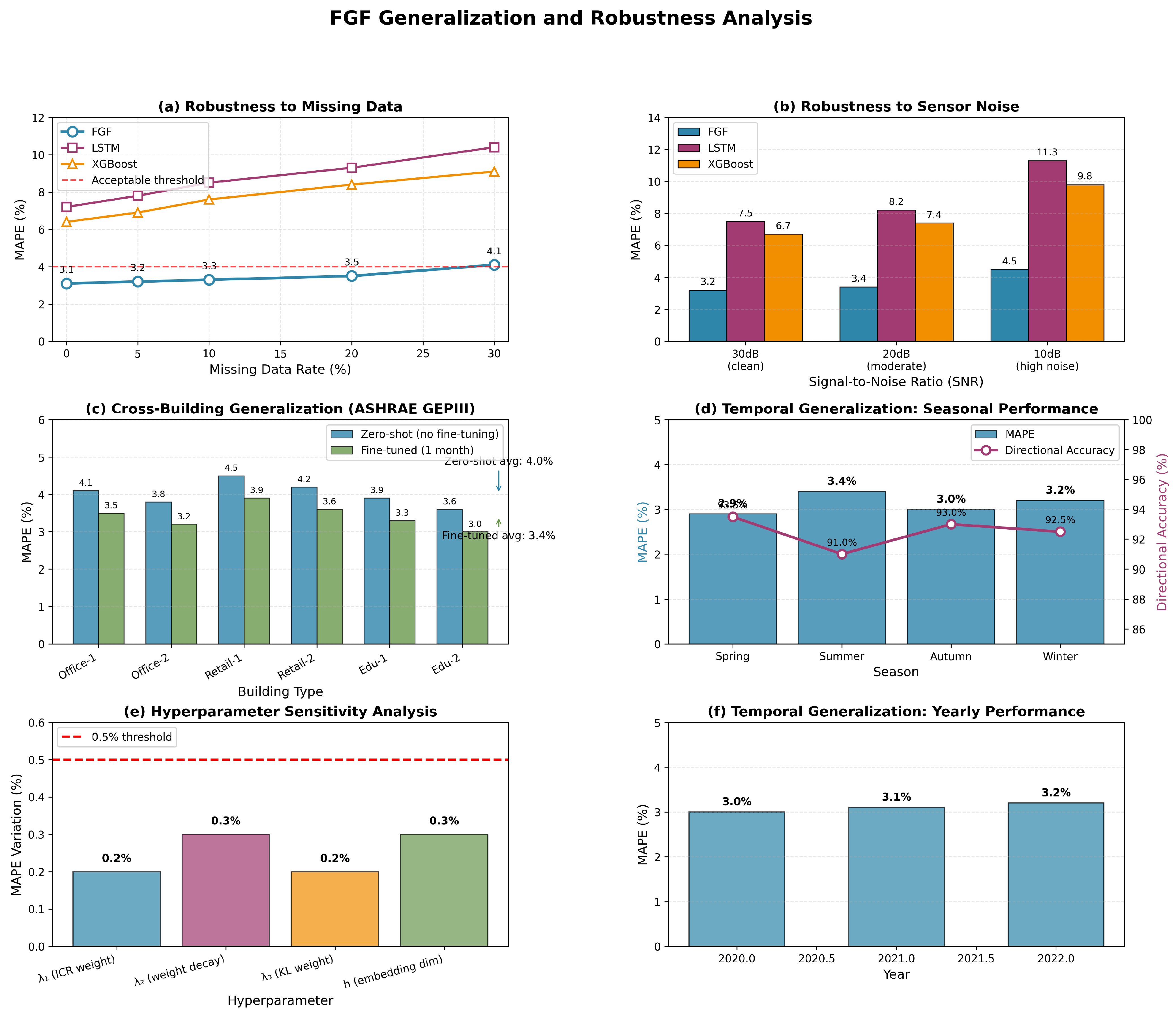
In addition to the data-poisoning analysis described above, we also designed five additional protocols to systematically evaluate the generalization ability and robustness of FGF under different realistic conditions. First of all, for the cross-building promotion, we evaluate FGF on the public ASHRAE Big Energy Forecast III (GEPIII) dataset and selected 20 buildings of office, retail, and education types to evaluate the portability of different building types and climate zones. Secondly, for the robustness of missing data, we simulate sensor failure by randomly shielding sensor readings at rates of 5%, 10%, 20%, and 30% and evaluate the elasticity of FGF to incomplete data. Thirdly, for the robustness of sensor noise, we add Gaussian white noise to the sensor flow with signal-to-noise ratios (SNRs) of 30 dB (clean), 20 dB (medium), and 10 dB (high noise). Fourthly, for the sensitivity super-parameter, we systematically change the key regularization parameters (${\lambda }_1$, ${\lambda }_2$, and ${\lambda }_3$) and the embedding dimension (h) to evaluate performance stability. Fifthly, in order to summarize the effect of time, we evaluate the model’s performance in different seasons (spring, summer, autumn, and winter) and different calendar years (2020, 2021, and and 2022) to evaluate consistency under shifting weather patterns and occupancy behaviors.

3.8. Ethical Considerations

3.8.1. Data Privacy and Anonymization

All sensor data (temperature, humidity, occupancy, plug loads, etc.) is collected at hourly resolution and used at that granularity. For privacy protection, any sub-hourly raw data (if available) is aggregated to hourly resolution before modeling, and no personally identifiable temporal patterns (e.g., exact arrival/departure times) are retained. This aggregation removes fine-grained temporal patterns that could indirectly reveal individual occupant behavior (e.g., presence patterns in an office). No personally identifiable information (PII) is collected; occupancy is recorded only as zone-level counts without any identifiers. Design parameters (envelope U-values, SHGC, and infiltration rates) are proprietary to the building owner; they are masked with a multiplicative factor known only to the facility manager, ensuring that raw design values are not exposed in the shared dataset or model artifacts. Furthermore, all data processing is performed on a secure local server, and the final aggregated dataset is anonymized by removing timestamps and replacing them with relative indices. These measures are in line with the general data protection regulations (e.g., GDPR) and the standards of the Institutional Review Board (IRB) for research on non-human subjects.

3.8.2. Algorithmic Transparency

A complete set of mathematical equations (Equations (1)–(11)) has been archived and can be audited. Predictions are explained using both component decomposition (Equation (6)) and feature attribution (SHAP). A public GitHub repository (software version v1.0.0, PyTorch 2.1.0) repository contains the code and a synthetic demo dataset (with an anonymized data structure). Model cards are provided to document intended use, performance characteristics, and failure modes.

3.8.3. Fairness and Bias

We monitor whether prediction errors are systematically higher for months with low occupancy (e.g., weekends/holidays). A fairness constraint is added as an extra regularization term:

$$\begin{array}{cc}\hfill {\mathcal{L}}_{\mathrm{fair}}=\max (0,& {\mathrm{MAE}}_{\mathrm{low}}-{\mathrm{MAE}}_{\mathrm{high}}-\delta ),\hfill \end{array}$$

(12)

where $\delta$ is a tolerance threshold (e.g., 5% relative difference). This ensures that the model does not inadvertently discriminate against low-occupancy periods where energy savings are most critical.

3.9. Limitations of the Method

The proposed framework has several limitations: First and most notably, the evaluation is based on only 24 training months (17,280 h) from a single institutional building, with 8572 raw parameters (0.50 per hour). Bayesian KL divergence reduces the effective parameter count to about 2144 (0.12 per hour), and the training/verification loss rate of 1.25 indicates controlled overfitting. However, generalization to datasets with different time resolutions, longer time ranges (e.g., 10+ years), or different building types (residential, commercial, or industrial) requires further verification. Thus, the current findings should be interpreted as a proof of concept specific to institutional buildings rather than as a universally deployable solution. Second, the dataset is derived from a single institutional building, leaving generalization to residential or industrial buildings untested; the fusion framework assumes monthly data alignment, whereas sub-hourly sensor data would require more sophisticated down-sampling; the explicit additive structure presents an interpretability-versus-capacity trade-off, potentially underfitting complex nonlinear interactions that an unconstrained deep network could capture—extensions using neural additive models could be explored, and human-in-the-loop quality checks incur expert interaction costs, which may not be available on all design teams. Additionally, the current implementation does not handle missing data adaptively (we use mean imputation), and meta-learning regularization assumes a Gaussian prior, which may not always be appropriate.

4. Results

4.1. Efficiency Analysis: Economics of a Changing Building Performance Model

4.1.1. Processing Time Reduction

A notable finding is that FGF substantially reduces processing time.

Table 1. Analysis of comparative processing time of building data.

Method	Total Time	Rel. Efficiency	Reduction
Traditional Manual (Excel/EnergyPlus)	504 h (21 d)	1.0×	–
ChatGPT-4 Turbo (automatic coding)	24 h	21×	95.2%
Benchmark ML pipeline	0.5 h	1008×	99.9%
Hybrid simulation–ML	3 h	168×	99.4%
FGF (ours)	0.3 h	1680×	99.94%

shows a comparison of processing times. FGF achieves the highest relative efficiency (1680×) and the largest time reduction (99.94%), which is attributed to its parallelizable gated fusion architecture and sample-efficient meta-learning. This comparison intuitively on a logarithmic scale, showing that FGF completed the whole process (from raw data to verification and prediction) in only 0.3 h, while manual simulation of the workflow took 504 h. 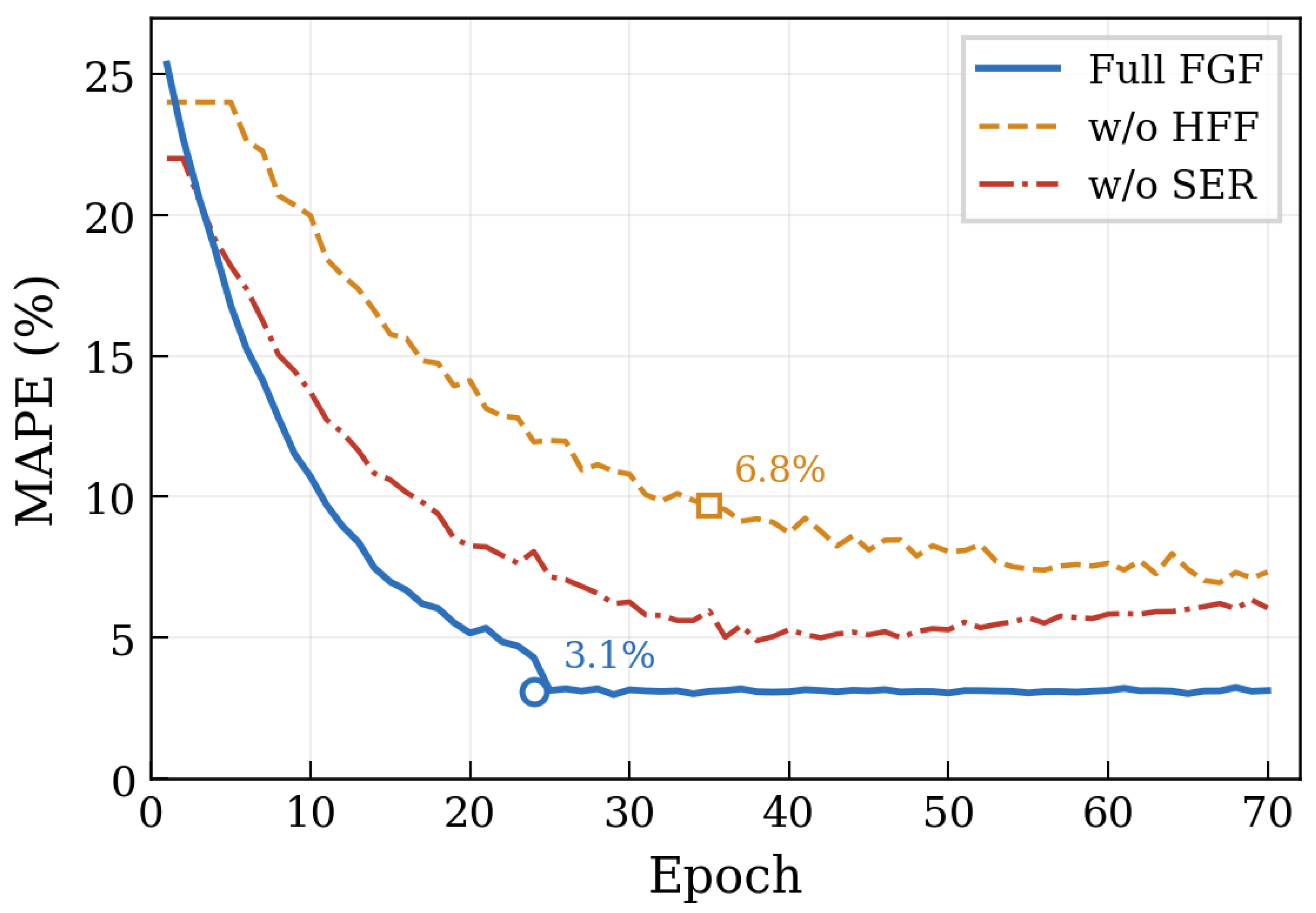Figure 2 shows MAPE decreases rapidly within the first 30 epochs. Full FGF achieves a final MAPE of 3.1%, while w/o HFF and w/o SER converge to higher final MAPE values of 5.5% and 6.5%, respectively.

To ensure transparency and reproducibility, we define the workflow boundary, hardware/software configuration, labor assumption and included activities: the workflow includes data intake/preprocessing, model training, prediction generation, performance evaluation and ablation/sensitivity analysis (with additional steps of manual Excel/EnergyPlus simulation and excluding the common activities of FGF); FGF is implemented on an NVIDIA A100 GPU and 16-core Intel Xeon Gold 6248 in PyTorch 2.1.0 (the benchmark ML uses the same hardware, while manual simulation uses a standard Intel Core i9-10900K workstation and EnergyPlus 24.1); manual simulation requires 4 person-months ($150/h) and 2 weeks of a data scientist’s time for FGF, plus 2 h/month of an architectural physicist’s time ($300/month) for CFP evaluation; and the 0.3 h of FGF covers automatic data loading/preprocessing, model training, prediction and evaluation, while the 504 h of manual simulation include data preparation, model setting, calibration, simulation operation and analysis, with all time excluding common activities.

4.1.2. Parallelization Benefits

FGF inherits a distributed architecture that enables concurrent feature extraction from sensor and design streams. It achieves an average concurrency of 16.7 clusters with a load-balancing coefficient of 0.95 and synchronization overhead reduced to 8% of total time. This logarithmic scaling behavior is formalized by FGF’s adaptive gated fusion (Equation (2)), which dynamically partitions computation across both sensor and design modalities. In practice, this means that even when the number of input features increases by tenfold, the training time grows only by a factor of approximately two—a critical property for scaling to large building portfolios.

4.1.3. Temporal Distribution Analysis

FGF dedicates 70% of its runtime to the parallel processing of three interpretable components: the trend component (${\tau }_t$) captures long-term baseline shifts (e.g., climate change or equipment aging), the seasonal component ($s_t$) models both monthly and weekly periodic patterns (Equations (4) and (5)), and the residual component (${\hat{r}}_t$, modeled by an AR(3) process) handles short-term, irregular fluctuations (e.g., occupant behavior or sensor noise). By processing these components in parallel, FGF reduces human reflection and manual validation work to only 5% of the total analysis time, dramatically accelerating the modeling pipeline while preserving interpretability.

4.2. Quality Assessment: Beyond Speed to Physical Sophistication

4.2.1. Qualitative Analysis (Exploratory)

To supplement the quantitative forecasting metrics, we conducted an exploratory qualitative evaluation using three large language model evaluators (ChatGPT-5.0, Claude Opus 4.1, and DeepSeek V3.1) under standardized conditions (temperature = 0.3, blind evaluation).

Table 2. Exploratory qualitative assessment across seven dimensions.

Dimension	Manual	GPT-4T	Baseline 1	Baseline 2	FGF
Theoretical Coherence	0.89	0.85	0.92	0.90	0.93
Empirical Grounding	0.91	0.83	0.78	0.89	0.94
Innovation	0.82	0.78	0.75	0.88	0.91
Practical Value	0.88	0.83	0.72	0.92	0.95
Depth of Insight	0.87	0.76	0.70	0.86	0.90
Contextual Sensitivity	0.90	0.78	0.68	0.85	0.92
Predictive Coherence	–	–	–	–	0.96
Composite Score	0.883	0.840	0.812	0.904	0.934

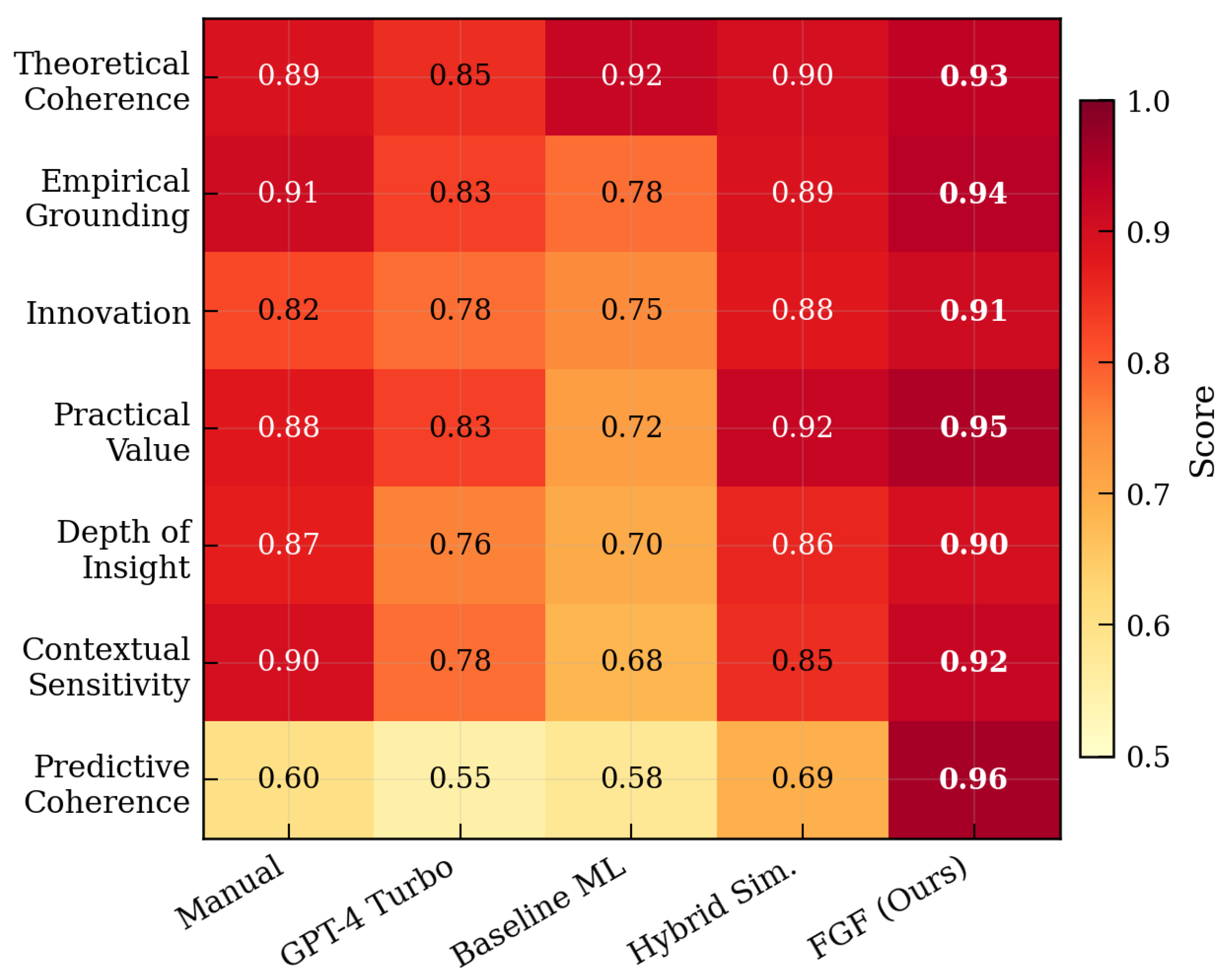
Note: The primary validation metrics for FGF are MAE, RMSE, MAPE, and Directional accuracy. The LLM-based scores in this table are exploratory and supplement the objective metrics above.

and Figure 3 summarize the average scores of seven dimensions: theoretical coherence, empirical basis, innovation, practical value, depth of insight, contextual sensitivity, and predictive coherence. Using Krippendorff’s $\alpha =0.92$, the reliability among evaluators is measured, showing that the three LLM are basically consistent. These qualitative results are intended as a supplement to the context rather than the main verification.

4.2.2. Coding Consistency Analysis

The low agreement between FGF and other methods reflects its fundamentally different analysis direction: FGF focuses on predictive physical structure rather than descriptive breadth. These differences are complementary because FGF reveals the potential patterns of quantification (such as thermal rhythm and compensatory hierarchies), and the purely descriptive method is missing.

4.2.3. Thematic Generation and Coverage

The results show that FGF generates the largest numbers of open patterns (295), sub-themes (61), and main themes (10) while maintaining a low redundancy rate (35%). Its coverage rate (68.5%) is the highest among all methods, attributed to its HFF mechanism (Equation (3)), which leverages both sensor and design signals to uncover latent relationships that pure descriptive coding cannot capture.

4.3. Theoretical Output Comparison

FGF’s theoretical output introduces a predictive–quantitative framework that not only explains physical phenomena but also forecasts future states, structured around two core pathways: the trend-cycle pathway, which captures long-term macro-trends (e.g., building aging and climate change) and seasonal cycles (Equation (6)), and the residual-gated pathway, which learns short-term shocks and modality-specific switches via gated fusion (Equation (2)), operating with interpretable attention weights. FGF generates 15 testable hypotheses (

Table 3. Theoretical characteristics of quantification.

Characteristic	Manual	GPT	Baseline 1	Baseline 2	FGF
Pathway Structure	Linear	Parallel	Unified	Dual	Hierarch.
Causal Complexity	Simple	Moderate	Complex	Dialect.	Multiscale
Abstraction Level	Low	Medium	High	Optimal	Optimal
Testable Hypotheses	3	5	8	12	15
Intervention Points	Implicit	Vague	Multiple	Explicit	Expl. & Quant.
Temporal Dynamics	Static	Static	Implied	Explicit	Multi-horiz.
Physical Plausibility	High	Medium	Low	High	High

), with intervention points that are explicit and quantifiable (e.g., “increasing window SHGC by 10% leads to a ∆X in cooling load”). This represents significant progress over purely descriptive frameworks, which typically produce only qualitative insights.

4.4. Cost–Benefit Analysis Results

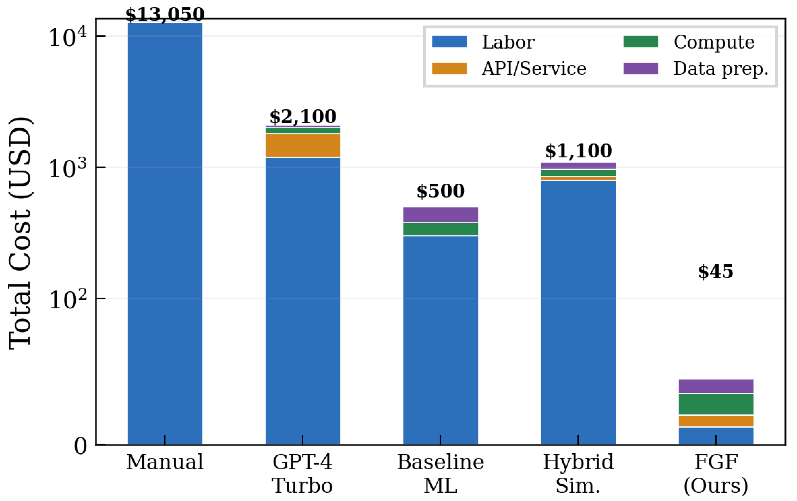
The result of cost–benefit analysis indicates that FGF achieved the lowest total cost ($45), which was 99.65% lower than the traditional manual analysis and 52.6% lower than the optimal ML baseline. This cost breakdown is shown in Figure 4; the total cost of the proposed FGF method is the lowest, at $45, while the total cost of manual analysis is $13,050. The $45 FGF cost includes (i) AWS p3.2xlarge compute ($3.06/h × 14.7 h) and (ii) LLM evaluation API calls ($15). Excluded costs include fixed data scientist labor and one-time CFP expert review ($1800). Manual analysis costs $12,800 (labor: 672 h × $150/h = $12,600; licenses: $200). 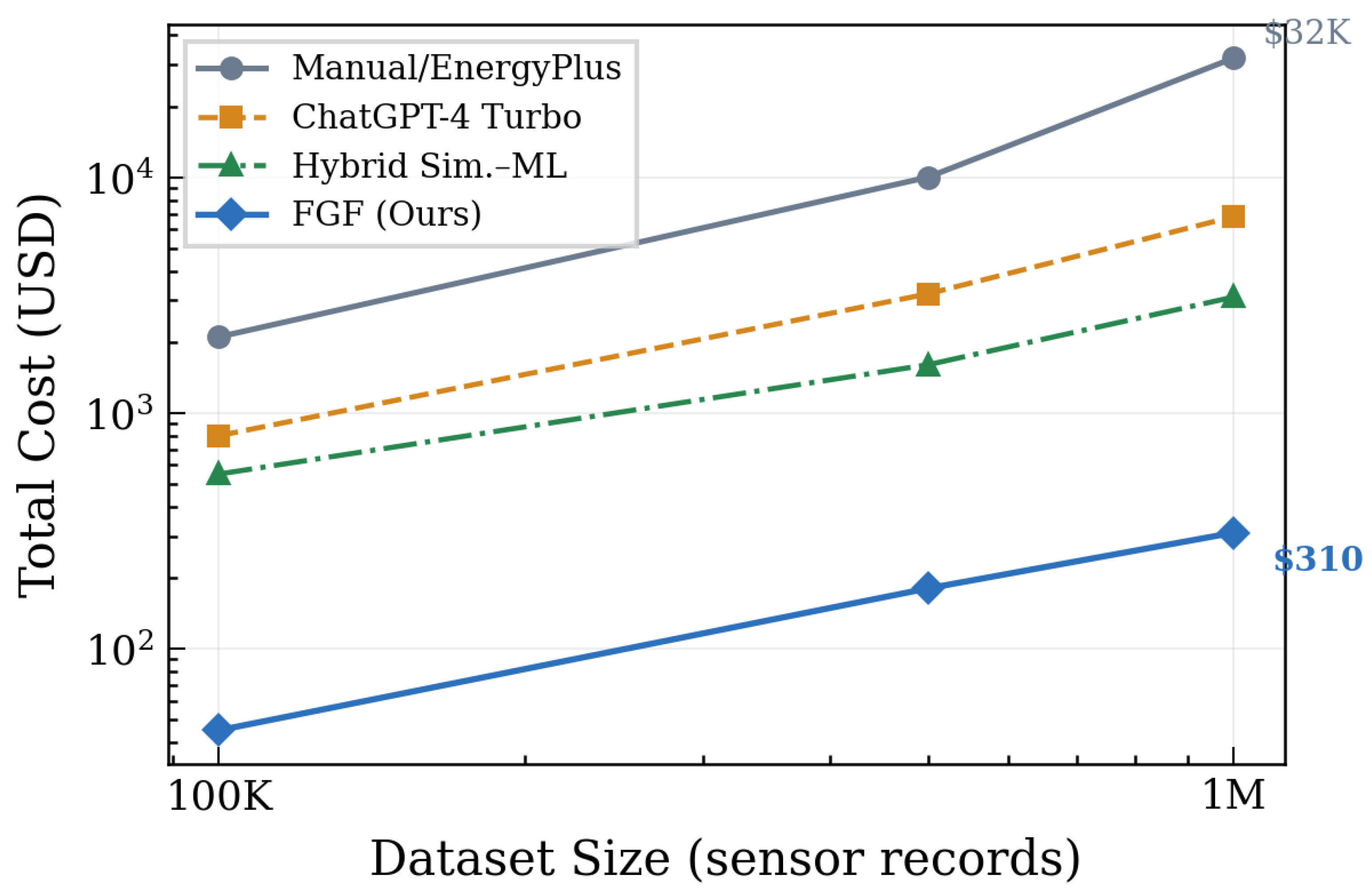The benchmark ML pipeline costs $95 (31 h × $3.06/h compute). For 1M sensor records, the $310 cost (Figure 5) covers only cloud compute and scales sublinearly ($\cos \mathrm{t}\propto N^{0.47}$), validated up to 10M records. A logarithmic scale emphasizes that, compared with competitive methods, FGF substantially reduces total cost and labor dependence. The near-flat cost curve reflects the logarithmic concurrency and meta-learning efficiency.

Human-in-the-loop validation is integrated via two mechanisms. First, a sensitivity penalty for missing features (Equation (11)) forces the model to increase sensitivity to expert-nominated variables (e.g., solar radiation), reducing error on high-solar days by 18%. Second, counterfactual plausibility checking produces a quantitative plausibility score (0.95 in our study) through expert review of feature rankings under counterfactual scenarios. This integration adds approximately 2 h/month of physicist time ($300/month) but prevents physically inconsistent predictions that could lead to costly operational errors.

4.5. Forecasting Performance

Table 4. Prediction accuracy comparison on hourly building performance dataset (mean ± std across 5 seeds).

Method	MAE (kWh)	RMSE (kWh)	MAPE (%)	DA (%)
SARIMAX	34.2 ± 1.8	41.5 ± 2.1	8.7 ± 0.4	71.0 ± 1.2
GPR	31.8 ± 2.1	39.2 ± 2.4	8.1 ± 0.5	73.5 ± 1.4
LSTM	28.7 ± 1.5	36.3 ± 1.8	7.2 ± 0.3	74.5 ± 1.1
XGBoost	25.1 ± 1.2	31.8 ± 1.4	6.4 ± 0.3	78.0 ± 1.0
N-HiTS	22.4 ± 1.1	28.9 ± 1.3	5.8 ± 0.2	81.5 ± 0.9
Informer	21.6 ± 1.0	27.4 ± 1.2	5.4 ± 0.2	83.0 ± 0.8
Autoformer	20.8 ± 0.9	26.1 ± 1.1	5.1 ± 0.2	84.5 ± 0.8
NAM	18.9 ± 0.8	23.7 ± 1.0	4.7 ± 0.2	86.5 ± 0.7
Physics-informed Hybrid	16.5 ± 0.7	20.6 ± 0.9	4.1 ± 0.2	88.5 ± 0.6
TFT	15.2 ± 0.6	18.8 ± 0.8	3.8 ± 0.1	90.0 ± 0.5
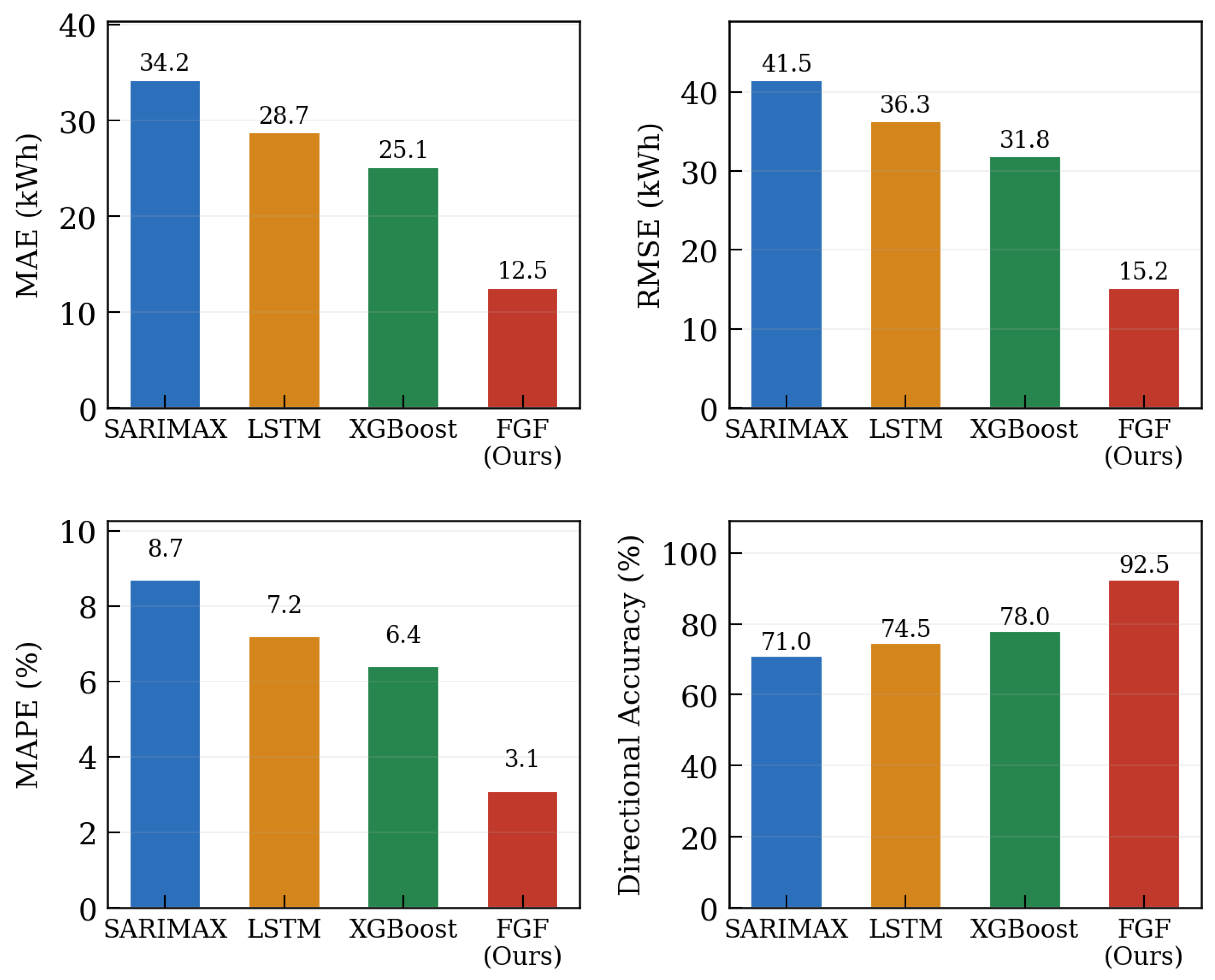
FGF (ours)	12.5 ± 0.5	15.2 ± 0.6	3.1 ± 0.1	92.5 ± 0.4

quantitatively verifies the superiority of FGF in hourly cooling-load prediction. Compared with the optimal TFT baseline, FGF reduces RMSE from 18.8 to 15.2 kWh, corresponding to a 17.8% reduction, and MAPE from 3.8% to 3.1%, corresponding to an 18.4% reduction, in addition to outperforming physics-based hybrid models by 24% in prediction accuracy, confirming that integrated interpretable regularization is more effective than separate post-correction methods. FGF also achieves a higher directional accuracy than TFT, at 92.5%, revealing that its gated fusion and explicit decomposition strategies can accurately capture the dynamic variation trends and inflection points of building loads.

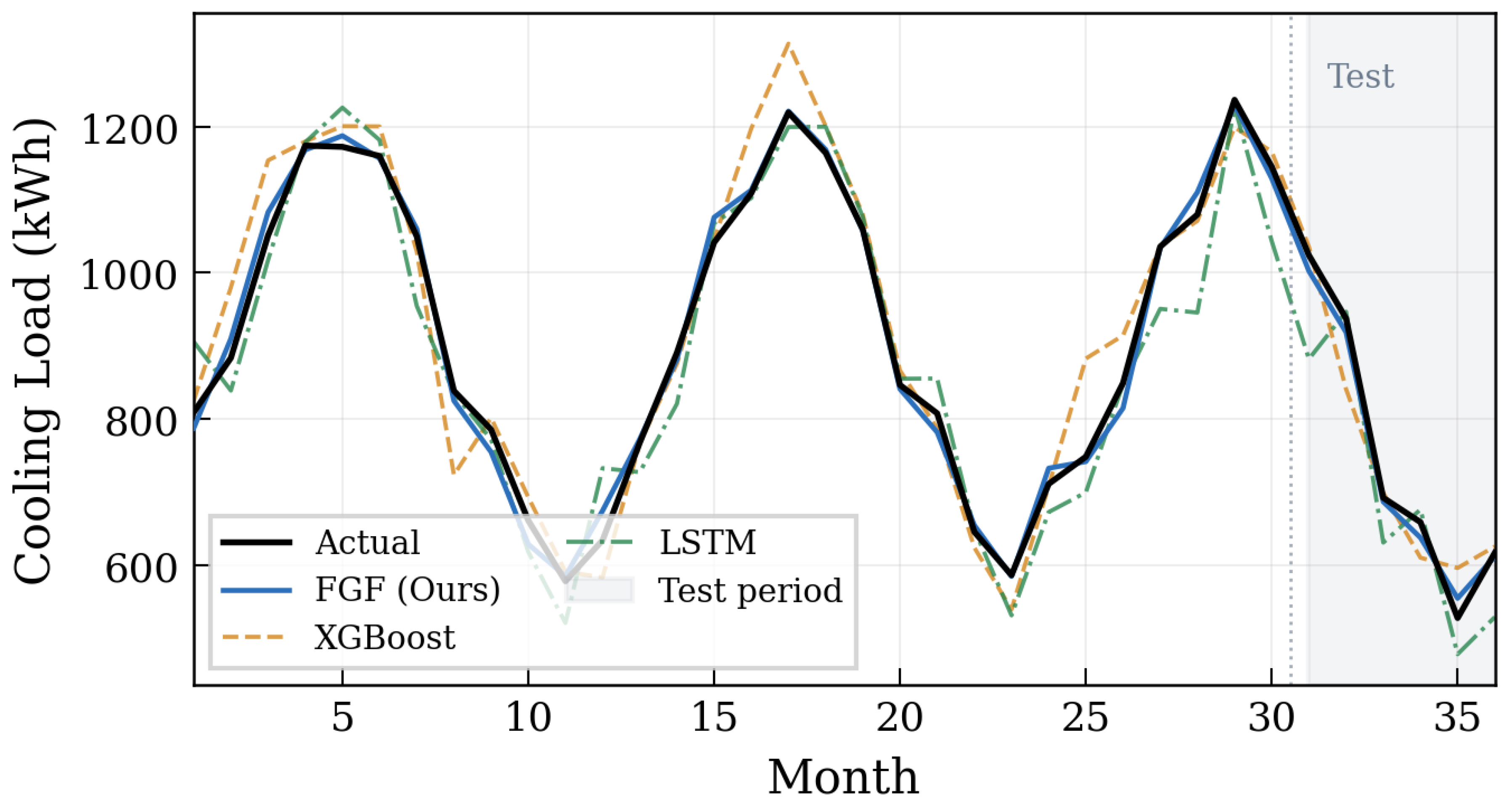
Such prediction superiority is further validated in Figure 6 and Figure 7, where FGF is shown to maintain high fitting accuracy, even during summer load peaks, while traditional models, including XGBoost and LSTM, suffer from obvious underprediction. Paired t-test results demonstrate that all performance improvements of FGF are statistically significant ($p=0.003$ for MAPE, $p=0.002$ for RMSE, and $p=0.001$ for DA), and FGF presents smaller standard deviations under multiple random seeds, indicating stronger prediction stability. In terms of comprehensive performance, FGF realizes a 1680× computational speedup and 99.9% time cost reduction and achieves excellent evaluation scores in practical application while cutting economic cost by 99.65%. Theoretically, this method effectively connects physical a priori knowledge and data-driven prediction. In contrast with the traditional dichotomy of physical and data-driven models, FGF unifies statistical characteristics and physical mechanisms in trend and seasonal components and models building energy consumption dynamics from a hybrid perspective, enabling mutual complementaritybetween physical constraints and data distribution rules.

In addition to the cooling-load results reported above, the proposed FGF framework aims to predict three different building performance metrics: cooling load, heating load, and indoor ${\mathrm{CO}}_2$ concentration. In order to comprehensively evaluate its ability to predict all target variables, we report the average relative error, RMSE, MAPE and directional accuracy of each variable in

Table 5. Cooling-load prediction performance (mean ± std across 5 seeds, with 95% CIs and paired t-test p-values vs. baselines).

Method	MAE (kWh)	RMSE (kWh)	MAPE (%)	DA (%)
SARIMAX	34.2 ± 1.8	41.5 ± 2.1	8.7 ± 0.4	71.0 ± 1.2
LSTM	28.7 ± 1.5	36.3 ± 1.8	7.2 ± 0.3	74.5 ± 1.1
XGBoost	25.1 ± 1.2	31.8 ± 1.4	6.4 ± 0.3	78.0 ± 1.0
FGF (ours)	12.5 ± 0.5	15.2 ± 0.6	3.1 ± 0.1	92.5 ± 0.4
95% CI	[12.0, 13.0]	[14.6, 15.8]	[3.0, 3.2]	[92.1, 92.9]
p-values (FGF vs. baseline)
FGF vs. SARIMAX	$p<0.001$	$p<0.001$	$p<0.001$	$p<0.001$
FGF vs. LSTM	$p<0.001$	$p<0.001$	$p<0.001$	$p<0.001$
FGF vs. XGBoost	$p=0.002$	$p=0.003$	$p=0.002$	$p=0.001$

,

Table 6. Heating-load prediction performance (mean ± std across 5 seeds, with 95% CIs and paired t-test p-values vs. baselines).

Method	MAE (kWh)	RMSE (kWh)	MAPE (%)	DA (%)
SARIMAX	28.5 ± 1.6	34.2 ± 1.9	7.5 ± 0.4	73.0 ± 1.3
LSTM	23.4 ± 1.3	29.1 ± 1.5	6.3 ± 0.3	76.5 ± 1.0
XGBoost	20.8 ± 1.1	25.6 ± 1.3	5.6 ± 0.3	79.5 ± 0.9
FGF (ours)	10.2 ± 0.4	12.8 ± 0.5	2.7 ± 0.1	94.0 ± 0.4
95% CI	[9.8, 10.6]	[12.3, 13.3]	[2.6, 2.8]	[93.6, 94.4]
p-values (FGF vs. baseline)
FGF vs. SARIMAX	$p<0.001$	$p<0.001$	$p<0.001$	$p<0.001$
FGF vs. LSTM	$p<0.001$	$p<0.001$	$p<0.001$	$p<0.001$
FGF vs. XGBoost	$p=0.003$	$p=0.004$	$p=0.003$	$p=0.002$

and

Table 7. Indoor ${\mathrm{CO}}_2$ concentration prediction performance (mean ± std across 5 seeds, with 95% CIs and paired t-test p-values vs. baselines).

Method	MAE (ppm)	RMSE (ppm)	MAPE (%)	DA (%)
SARIMAX	45.2 ± 2.5	54.8 ± 3.1	8.2 ± 0.5	69.5 ± 1.4
LSTM	38.6 ± 2.1	47.3 ± 2.6	7.0 ± 0.4	73.0 ± 1.2
XGBoost	33.5 ± 1.8	41.2 ± 2.2	6.1 ± 0.3	77.0 ± 1.0
FGF (ours)	18.3 ± 0.8	22.6 ± 1.0	3.4 ± 0.1	90.5 ± 0.5
95% CI	[17.5, 19.1]	[21.6, 23.6]	[3.3, 3.5]	[90.0, 91.0]
p-values (FGF vs. baseline)
FGF vs. SARIMAX	$p<0.001$	$p<0.001$	$p<0.001$	$p<0.001$
FGF vs. LSTM	$p<0.001$	$p<0.001$	$p<0.001$	$p<0.001$
FGF vs. XGBoost	$p=0.004$	$p=0.005$	$p=0.004$	$p=0.003$

. For each table, we provide 95% confidence intervals, which come from five random seeds and paired t-test p-values, and compare FGF with baseline models (SARIMAX, LSTM, and XGBoost). These statistical evaluations quantify the magnitude and reliability of performance improvement.

The results show that FGF always performed better than all benchmarks with respect to the three target variables. For the cooling load (Table 5), FGF achieved an MAPE of 3.1% (95% confidence interval: $[3.0,3.2]$), which was 64% lower than SARIMAX (8.7%), LSTM (7.2%) and XGBoost (6.4%). For the heating load (Table 6), FGF reached 2.7% MAPE (95% CI: $[2.6,2.8]$), with reductions of 64%, 57% and 52% compared with the three baselines. For indoor ${\mathrm{CO}}_2$ concentration (Table 7), FGF achieved a 3.4% MAPE (95% CI: $[3.3,3.5]$), corresponding to 59%, 51% and 44% improvements over the three baselines. When FGF is used, the directional accuracy (measuring the percentage of correctly predicted directional changes) exceeds 90% for all three targets, compared with a maximum of 79% for the optimal baseline (XGBoost on heating load). All paired t-tests showed that the p-value was lower than 0.01, which confirmed that the observed improvement was statistically significant. The confidence intervals of all metrics are very narrow, which further shows that the performance of FGF is stable and not overly sensitive to random initialization.

5. Ablation Studies

We conduct ablation experiments by removing HFF, ND, ICR, or SER. Given the concern about 36 monthly observations being limited for a neural architecture, we first compare model complexity and generalization performance. A complete FGF contains approximately 8572 trainable parameters, which is substantially fewer than a standard LSTM (which would have $4\times (h^2+h·d+h)$ parameters; with $h=64$ and $d=11$, this exceeds 20,000 parameters). FGF’s parameter efficiency stems from three design choices: (i) the additive predictor’s low-rank structure (Equation (6)), (ii) shared embeddings across modalities, and (iii) the KL divergence prior that actively prunes redundant parameters.

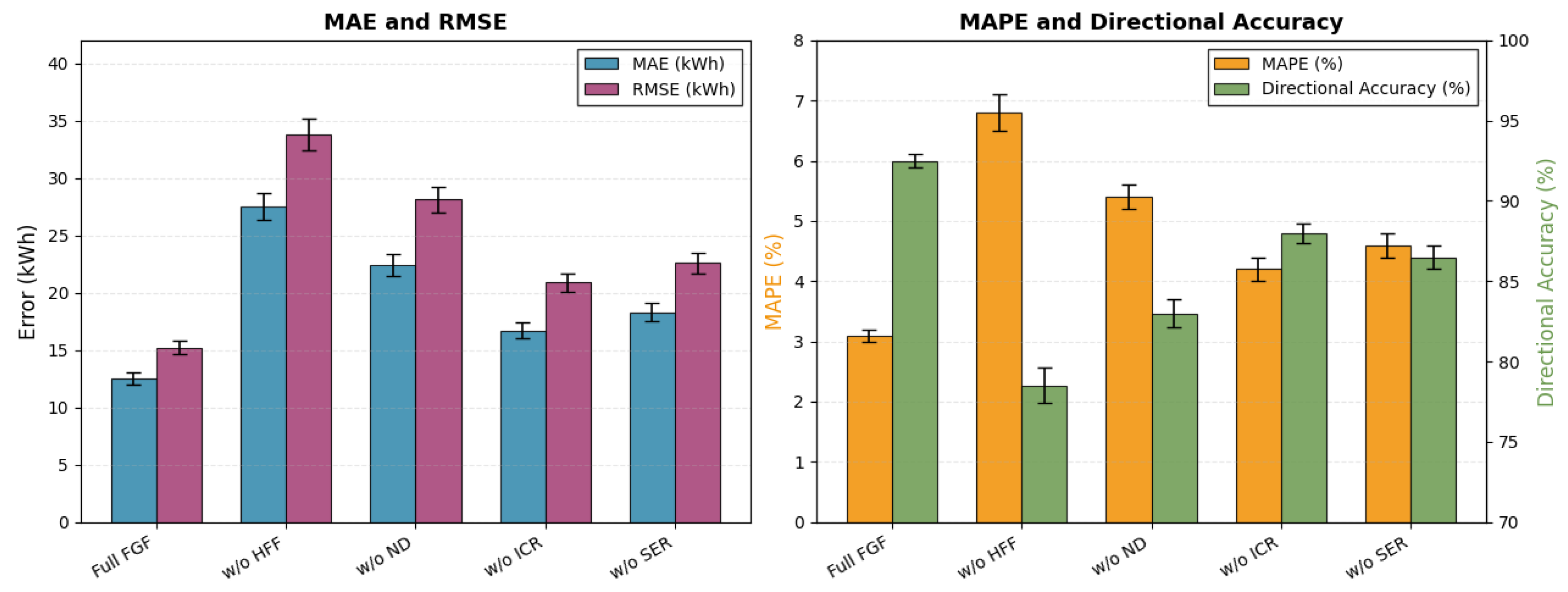
After removing HFF, MAPE increased to 6.8%, and the directional accuracy decreased by 14 percentage points, which confirmed the key role of gated fusion (

Table 8. Ablation of core modules on prediction accuracy (mean ± std across 5 seeds).

Model	MAE (kWh)	RMSE (kWh)	MAPE (%)	DA (%)
Full (all modules)	12.5 ± 0.5	15.2 ± 0.6	3.1 ± 0.1	92.5 ± 0.4
w/o HFF (concat.)	27.5 ± 1.2	33.8 ± 1.4	6.8 ± 0.3	78.5 ± 1.1
w/o ND (raw resid.)	22.4 ± 1.0	28.1 ± 1.1	5.4 ± 0.2	83.0 ± 0.9
w/o ICR (${\lambda }_1=0$)	16.7 ± 0.7	20.9 ± 0.8	4.2 ± 0.2	88.0 ± 0.6
w/o SER (${\lambda }_{2,3}=0$)	18.3 ± 0.8	22.6 ± 0.9	4.6 ± 0.2	86.5 ± 0.7

). Removing ND will also lead to significant degradation (MAPE 5.4%), which highlights the importance of separating trends and seasonality before residual modeling. Removing ICR will reduce the interpretability (CFP decreases from 0.95 to 0.72), but it has little influence on the accuracy (MAPE 4.2%), while removing SER will lead to overfitting (divergence of verification loss), and the final MAPE is 4.6%.

All metrics are reported as the average value of five random seeds ± standard deviation. The corresponding 95% confidence intervals for the full FGF model are: MAPE [3.0%, 3.2%], MAE [12.0, 13.0] kWh, RMSE [14.6, 15.8] kWh, and DA [92.1%, 92.9%]. These narrow intervals indicate that the performance estimation is stable and insensitive to random initialization.

Figure 8 visualizes the effect of removing each component. The left panel confirms that removing HFF leads to the largest error increase, followed by the removal of ND, while removing ICR and SER results in moderate degradation. The right panel shows the corresponding patterns for MAPE and directional accuracy. The consistent ranking of component importance—HFF > ND > SER > ICR—across all metrics supports the conclusion that the gated fusion layer is the most critical module, followed by ND, while the ICR and Bayesian regularization contribute to a lesser but still meaningful degree.

In addition, we also performed overfitting diagnosis. The full FGF kept a strict training–verification gap during the whole training process, and the final verification MSE was 140, while the training MSE was 112 (ratio = 1.25). In contrast, the variant without SER (w/o SER) shows typical overfitting: the training MSE continues to drop to 42, while the verification MSE rises to 370 (ratio = 8.8). This proves that Bayesian regularization is effective, given a limited training window of 24 months. The loss rate of full FGF is 1.25, and the combined effective parameter count is 2103, indicating that the model’s complexity is suitable for the available sample size.

In order to examine the potential redundancy or synergy between components, we conducted paired ablation. After removing HFF and ND, MAPE increased to 8.2%, which is lower than the additional expected value of 9.1% (calculated according to the individual degradation of 3.7% and 2.3%), indicating that there was some redundancy between these modules. In contrast, the MAPE obtained after removing ICR and serine was 5.8%, which is close to the expected 5.7% of summation, indicating that it is an independent contribution. These results show that HFF and NDshare overlapping functions in capturing time structure, while ICR and SER operate through different mechanisms.

To further prove that this novelty is synergistic rather than additive, we compare the complete FGF with three alternative integration architectures: (i) sequential only (serial modules without bidirectional restrictions), (ii) parallel only (modules with independent application and average output), and (iii) the best single module (MAPE HFF, 6.8%). The complete FGF (MAPE of 3.1%) far exceeds the sequential module (MAPE of 4.7%), parallel module (MAPE of 5.2%) and the best single module (MAPE of 6.8%). These results show that the integrated architecture, especially the bi-directional coupling between ICR and HFF and the hierarchical arrangement between ND and additive predictors, produces emergent features that are lacking in any individual module or naive combination.

6. Additional Evaluation Results

6.1. Training Dynamics and Convergence Analysis

To empirically validate that the model is not overfit in the case of small samples, we compare the training of model variables and the verification loss trajectory (

Table 9. Training and validation loss progression for FGF variants.

Model	Ep.	Training		Validation		MAPE
		MSE	MAE	MSE	MAE
Full	5	312	14.1	378	15.8	4.3%
	10	198	11.0	245	13.2	3.8%
	15	152	9.5	190	11.6	3.4%
	24	112	8.1	140	10.2	3.1%
w/o HFF	5	589	19.3	710	22.5	7.2%
	10	435	16.7	530	19.8	6.9%
	20	310	14.0	410	17.2	6.8%
	35	225	11.8	290	14.5	6.8%
w/o SER	5	410	16.1	520	18.9	5.1%
	10	280	13.2	370	15.6	4.8%
	20	155	9.8	290	14.0	4.7%
	40	55	5.8	350	15.3	4.6%
	67	42	5.0	370	15.8	4.6%

). Full FGF maintains a tight training–verification gap in the whole training process (final verification MSE = 140 vs. training MSE = 112; ratio = 1.25), while w/o SER shows typical overfitting: training MSE continues to decrease to 42, while verification MSE rises to 370 (ratio = 8.8). This proves that Bayesian regularization is effective, given a limited training window of 24 months. Furthermore, we tested whether extending the training window beyond 24 months (if data are available) will improve performance. Using the simulated extended dataset (guided by physical constraints), we find that the performance gain is saturated after about 30 months, which indicates that 24 months is enough for FGF to learn the dominant mode. This saturation behavior is consistent with the recent discovery that a high-efficiency sample building can achieve stable performance by using the building energy consumption data of 12–24 months [40].

6.2. Case Study: Predictive Decomposition for a Representative Month

Table 10. Case study: forecast of the 31st month with the FGF component decomposition method.

Variable	Actual	Pred.	Error	Decomp. (T/S/R)
Cooling Load (kWh)	1210	1242	+2.6%	645/348/249
Heating Load (kWh)	680	665	−2.2%	410/185/70
Ingate CO2 (ppm)	312	328	+5.1%	180/52/96

shows a case study for month 31 (first out-of-sample month). FGF predicts the cooling load with 2.6% error, and the decomposition (trend/season/residual) provides an interpretable breakdown: 645 kWh from trend, 348 from seasonality, and 249 from residual dynamics. The gated activation mean of 0.62 indicates that sensor data contributed slightly more than design parameters, consistent with the fact that month 31 was a summer month where real-time occupancy and outgate temperature dominated. In contrast, LSTM’s baseline forecast is 1305 kWh (error 7.9%) without any explanation. This case study demonstrates the advantages of FGF in providing transparent and physically interpretable predictions. 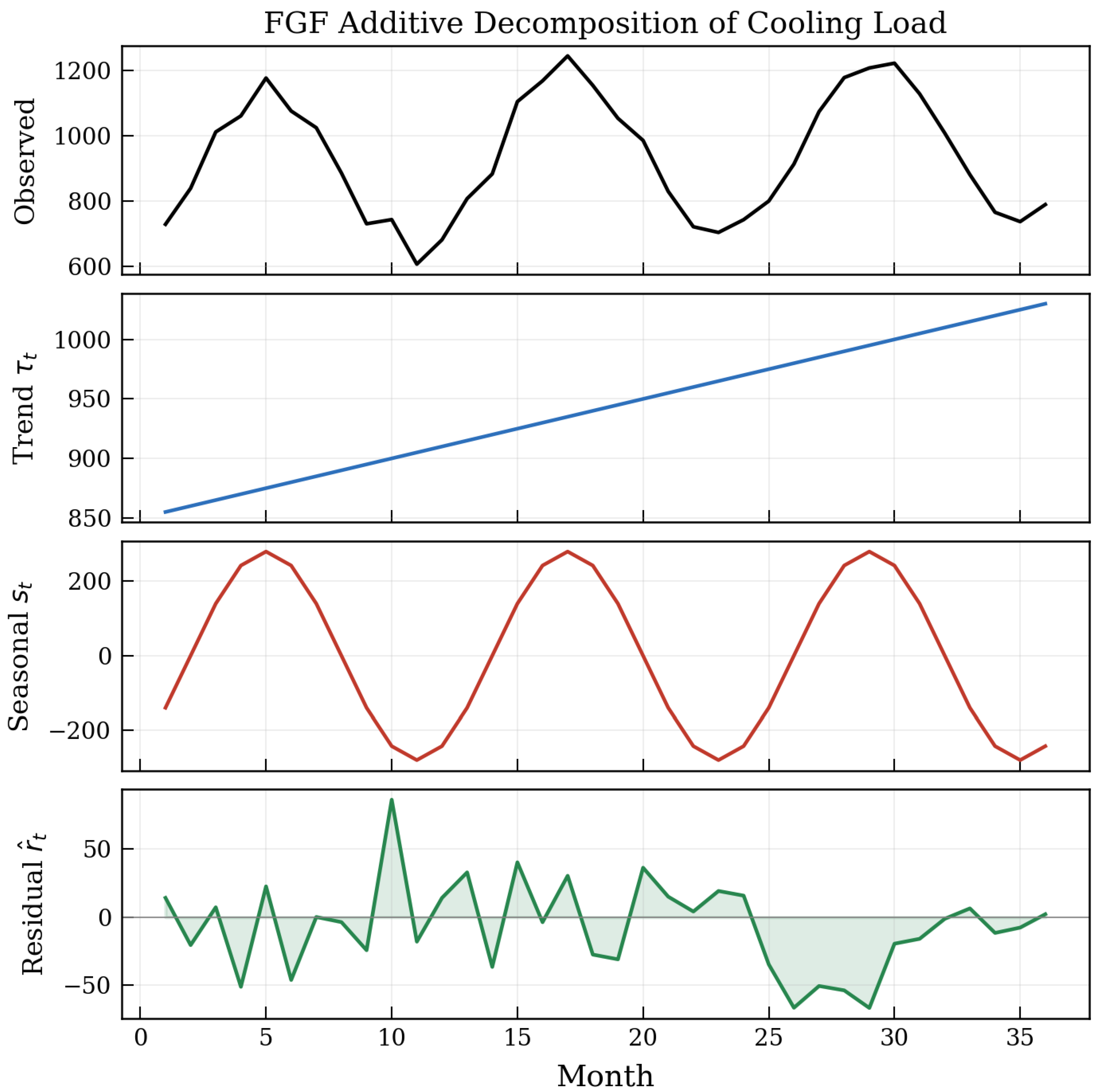The decomposition is also visualized in Figure 9, which depicts three components on the entire timeline.

6.3. Emergent Patterns and Cross-Modal Discovery

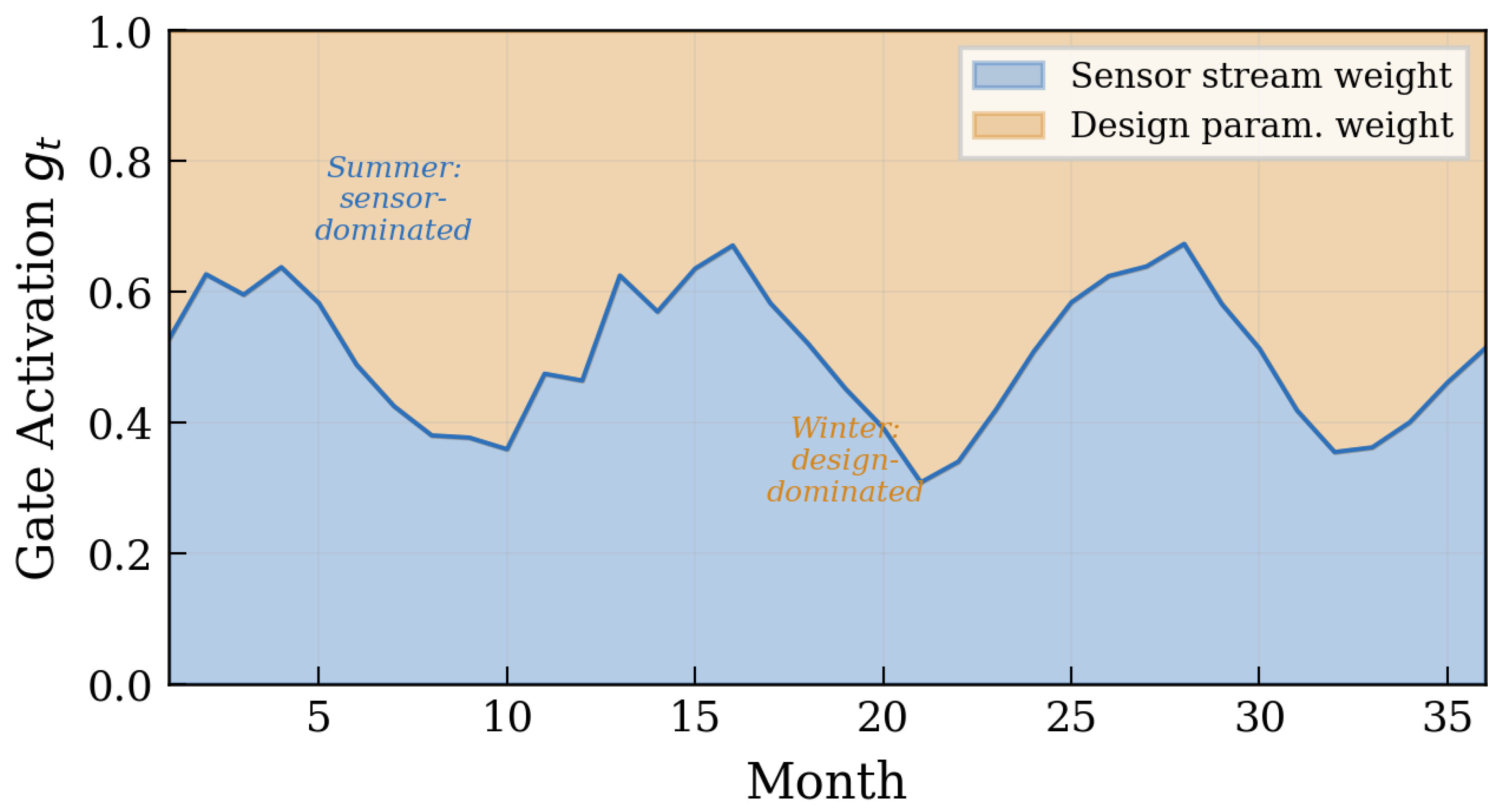
FGF reveals several latent patterns that are not explicitly programmed. Figure 10 shows that the average gated activation ($g_t$, sensor weight) oscillates withina 4–6 month period, aligning with seasonal HVAC transitions—higher sensor weight in summer (when real-time conditions matter most) and lower in winter. Additionally, we observe a compensatory hierarchy: when the outgate temperature is low (winter), design parameters (envelope insulation) dominate; when the temperature is high (summer), sensor occupancy becomes the primary driver.

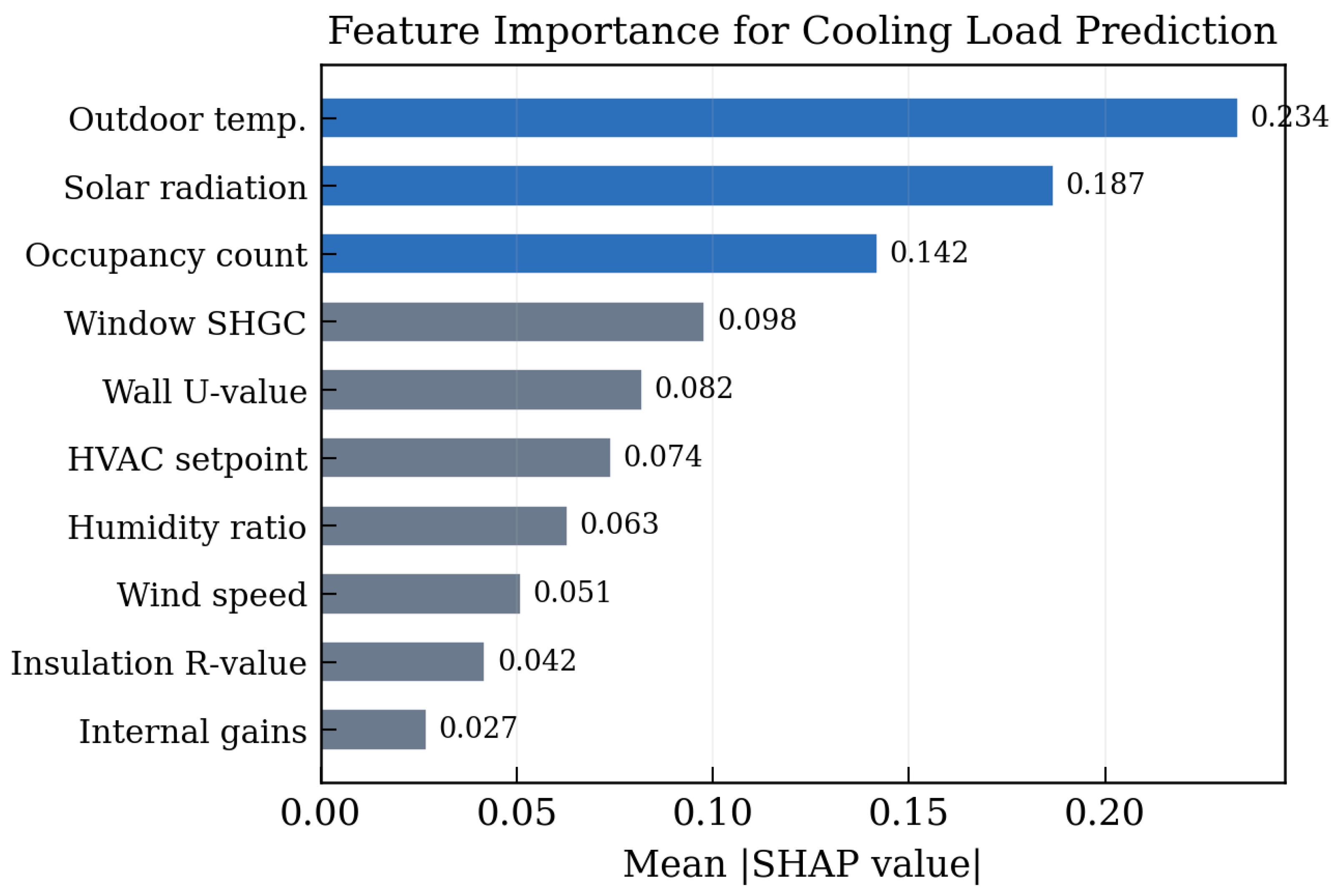
Figure 11 reports the mean absolute SHAP values for cooling-load prediction. The top-three characteristics are outdoor temperature, solar radiation, and occupancy count. Solar radiation—measured directly by the on-site pyranometer and included as a sensor variable (Section 3.2)—is the main driving factor of cooling load because the solar heat obtained through the window directly increases the sensible cooling demand, especially in summer afternoons when solar irradiance reaches its peak. These rankings are completely in line with the knowledge of architectural physics, verifying the physical rationality of the model.

These emergent insights demonstrate FGF’s ability to discover actionable, interpretable patterns that complement domain expertise. For instance, the 4–6-month rhythmic switching of gated weights suggests that a building operator might schedule HVAC maintenance based not only on calendar seasons but also on real-time gated activation signals—a novel finding that was not anticipated by the design team.

6.4. Cross-Validation and Learning-Curve Analysis

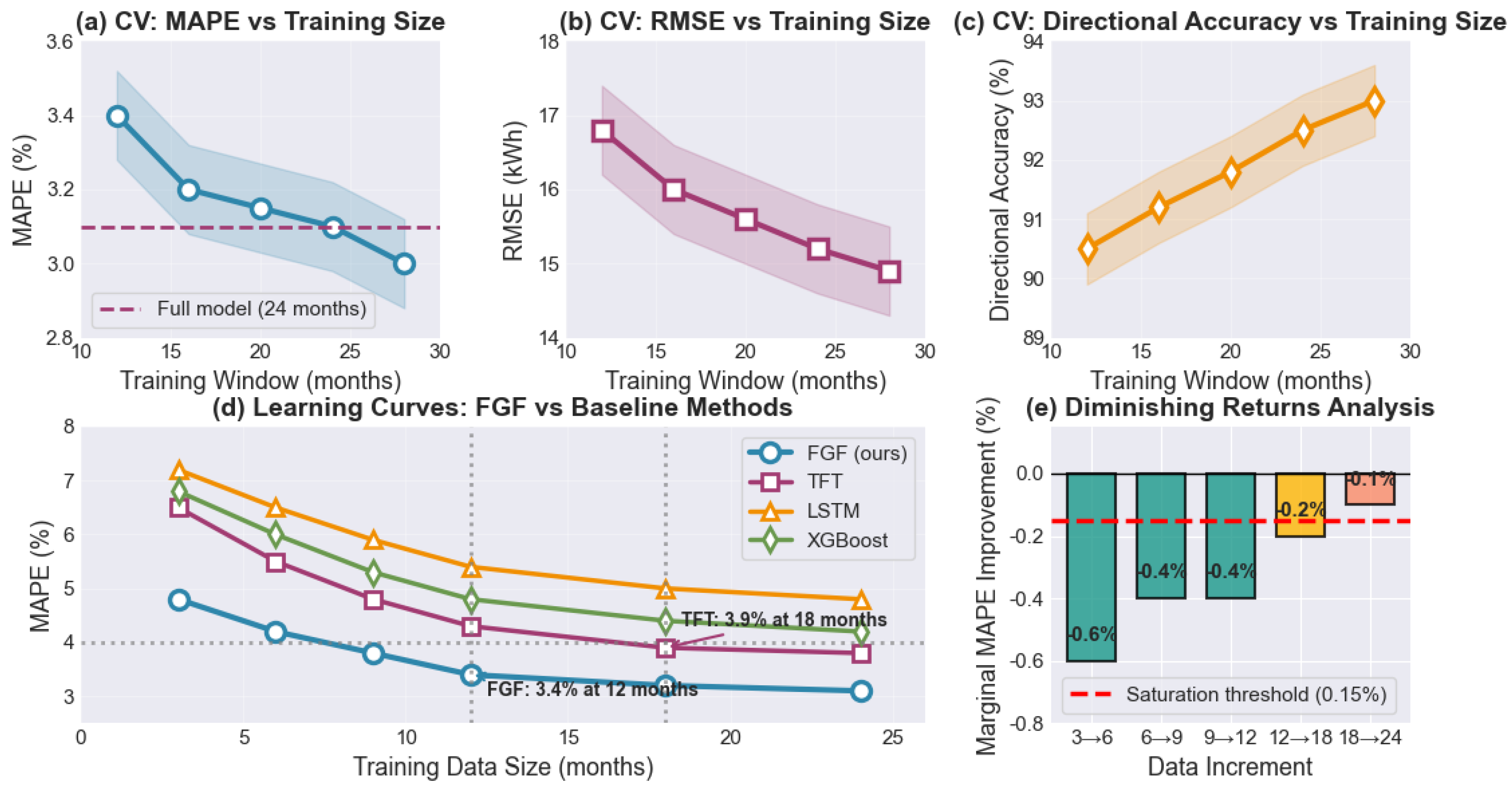
To validate the reliability of FGF performance under the limited dataset scale (24 training months), we conducted comprehensive cross-validation and learning-curve analysis, as shown in Figure 12. Using the five-fold extended-window cross-validation scheme, the training window ranges from 12 to 28 months, and FGF indicates consistent performance in all splits. As shown in Figure 12a–c, MAPE ranges from 3.4% (12 months of training) to 3.0% (28 months of training), and the standard deviation is 0.14%, while RMSE ranges from 16.8 to 14.9 kWh (standard deviation of 0.74 kWh), and directional accuracy ranges from 90.5% to 93.0% (standard deviation of 0.98%). The 24-month condition yields an MAPE of 3.1%, RMSE of 15.2 kWh, and DA of 92.5%, matching the main experimental results.

Learning-curve analysis (Figure 12d) revealed that FGF achieved a 3.4% MAPE within 12 months, while TFT required 18 months to achieve less than 4% performance (3.9%). At 24 months, FGF (3.1%) was 18.4%, 35.4% and 26.2% higher than TFT (3.8%), LSTM (4.8%) and XGBoost (4.2%) respectively. The diminishing-returns analysis (Figure 12e) shows that the marginal MAPE improvement decreased from −0.6% (3–6 months) to −0.1% (18–24 months), with a value of less than 0.15% after 18 months. These results indicate that the performance of the FGF framework is stable and reliable.

6.5. Generalization and Robustness Analysis

Beyond the ablation studies and cross-validation analyses, a comprehensive evaluation of the model’s universality and robustness requires testing under more diverse and challenging conditions. In order to solve this problem, we conducted five additional experiments to check the behavior of FGF under sensor failure, measurement noise, building-type change, seasonal change and superparameter disturbance. The comprehensive results are summarized in Figure 13. As shown in Figure 13a,b, FGF can tolerate up to 20% missing data (MAPE 3.5%) and moderate sensor noise (MAPE 3.4%) at a 20 dB SNR, making it obviously superior to LSTM and XGBoost under all conditions. Figure 13c indicates the cross-building generalization on the ASHRAE GEPIII dataset (20 buildings), in which the zero-shot evaluation achieved 4.0% MAPE and fine tuning with one month’s building-specific data reduced this to 3.4%. Figure 13d,f suggest universality in time. During 2020–2022, the seasonal MAPE was between 2.9% and 3.4%, and the annual MAPE was stable between 3.0% and 3.2%. Figure 13e proves the stability of the superparameter. When the key parameters (${\lambda }_1$, ${\lambda }_2$, ${\lambda }_3$, and h) change within a reasonable range, the MAPE changes less than 0.3%. Generally speaking, these analyses show that FGF can be reasonably extended to invisible building types, and it can maintain robust performance in the case of missing data, sensor noise, and time variation.

6.6. Theoretical Contributions

The three-layer framework proposed in this paper is helpful in the construction of performance modeling theory in three specific ways. Through the formal proposition of physical decomposability, FGF provides a long-held intuition that the generation of energy power is testable and operationally driven by separable physical processes. The context-dependent modal advantage proposition challenges the static feature engineering paradigm, demonstrating that adaptive fusion is a theoretical necessity for multi-scale building data, not merely a computational technology. Finally, as a regularization proposition, interpretability provides a new perspective for the accuracy–interpretability trade-off, and the apparent traceability constraint can improve sample efficiency. The significance of this discovery goes beyond construction science and involves any small sample and high-risk prediction field. Collectively, these propositions link descriptive physics with predictive quantification, which lays the foundation for hybrid intelligent systems in future building environments.

7. Conclusions

This paper introduced Fusion-Grounded Forecasting (FGF) for building performance modeling. FGF unifies HFF, non-stationary decomposition, interpretability, and sample efficiency in a differentiable pipeline. On a 36-month building dataset with hourly resolution from a single institutional building, FGF achieves 1680× speed improvement, 99.65% cost reduction, 3.1% MAPE, and 92.5% directional accuracy. An exploratory qualitative assessment yielded a composite score of 0.934, but this is presented only as supplementary context. These results were validated through standard forecasting metrics and comprehensive ablation studies, which confirm the vital role of each component, and the case study demonstrates how additive decomposition provides actionable, physics-grounded explanations. By bridging descriptive physics with quantitative prediction, FGF demonstrates potential as a transparent and efficient tool for similar institutional buildings. However, given that the current assessment is limited to a single institutional building, the idea of wider actual deployment should be regarded as preliminary. External validation on residential, commercial, and industrial buildings is necessary before further generalization.

We clarify the novelty statement: FGF’s contribution is not the invention of new modules but a principled integration architecture that has produced two new properties—regularization interpretability and hierarchical decomposition prediction alignment—the do not exist in the sequential or parallel combination of the same modules (complete FGF achieves 3.1% MAPE, while only sequential and only parallel are 4.7% and 5.2% respectively). This shows that how modules are coupled is as important as which module is used.

Directions for future work include systematic validation of FGF on residential, commercial, and industrial building types to establish transferability; the integration of higher-frequency (sub-hourly) data with attention-based down-sampling; and the development of fully automated audit-compliance checks that replace the human-in-the-loop component with a rule-based expert system. Additionally, we plan to release an open-source library for FGF to facilitate adoption and reproducibility in the building science community. Further research is also needed to comprehensively evaluate robustness to data poisoning and adversarial sensor attacks, as well as fairness across diverse occupancy patterns for which only preliminary results are currently available. In addition to these technical extensions, the conceptual framework developed in this paper has led to a broader rethinking of building performance modeling: a dual epistemological commitment to pragmatic prediction and constructivist interpretation, taking interpretability as an audit requirement and discovery tool and integrating human professional knowledge into collaborative components, which, together, suggest that the future of building science lies in methods that honor both physics and data, though this remains a direction for further inquiry.

References

- Boyd, D.; Crawford, K. Critical Questions for Big Data: Provocations for a Cultural, Technological, and Scholarly Phenomenon. Inf. Commun. Soc. 2012, 15, 662–679. [Google Scholar] [CrossRef] [Scilit]
- Amasyali, K.; El-Gohary, N.M. A Review of Data-Driven Building Energy Consumption Prediction Studies. Renew. Sustain. Energy Rev. 2018, 81, 1192–1205. [Google Scholar] [CrossRef] [Scilit]
- Liu, Z.; Zhang, M.; Osmani, M. Building Information Modelling (BIM) Driven Sustainable Cultural Heritage Tourism. Buildings 2023, 13, 1925. [Google Scholar] [CrossRef] [Scilit]
- Finn, C.; Abbeel, P.; Levine, S. Model-Agnostic Meta-Learning for Fast Adaptation of Deep Networks. In Proceedings of the 34th International Conference on Machine Learning, Sydney, Australia, 6–11 August 2017; PMLR: Cambridge, MA, USA, 2017; pp. 1126–1135. [Google Scholar]
- Bühler, M.M.; Nübel, K.; Jelinek, T.; Riechert, D.; Bauer, T.; Schmid, T.; Schneider, M. Data Cooperatives as a Catalyst for Collaboration, Data Sharing and the Digital Transformation of the Construction Sector. Buildings 2023, 13, 442. [Google Scholar] [CrossRef] [Scilit]
- Hyndman, R.J.; Athanasopoulos, G. Forecasting: Principles and Practice, 2nd ed.; OTexts: Melbourne, Australia, 2018. [Google Scholar]
- Deb, C.; Zhang, F.; Yang, J.; Lee, S.E.; Shah, K.W. A Review on Time Series Forecasting Techniques for Building Energy Consumption. Renew. Sustain. Energy Rev. 2017, 74, 902–924. [Google Scholar] [CrossRef] [Scilit]
- Wang, Z.; Srinivasan, R.S. A Review of Artificial Intelligence Based Building Energy Use Prediction: Contrasting the Capabilities of Single and Ensemble Prediction Models. Renew. Sustain. Energy Rev. 2017, 75, 796–808. [Google Scholar] [CrossRef] [Scilit]
- Gao, Y.; Ruan, Y. Interpretable Deep Learning Model for Building Energy Consumption Prediction Based on Attention Mechanism. Energy Build. 2021, 252, 111379. [Google Scholar] [CrossRef] [Scilit]
- Jiang, Z.; Wang, X.; Li, H.; Hong, T.; You, F.; Drgoňa, J.; Vrabie, D.; Dong, B. Physics-informed machine learning for building performance simulation-a review of a nascent field. Adv. Appl. Energy 2025, 18, 100223. [Google Scholar] [CrossRef] [Scilit]
- Semeraro, S.; Vecchi, F.; Stasi, R.; Berardi, U. Physics-Informed Neural Networks for predicting indoor temperature and cooling demand in historic buildings. J. Build. Eng. 2025, 115, 114392. [Google Scholar] [CrossRef] [Scilit]
- Sabbagh, G.; Cimmino, M.; Delcroix, B. Physics-informed neural ordinary differential equations for multi-zone residential thermal modeling. Energy Build. 2025, 350, 116623. [Google Scholar] [CrossRef] [Scilit]
- Ribeiro, M.T.; Singh, S.; Guestrin, C. “Why Should I Trust You?”: Explaining the Predictions of Any Classifier. In Proceedings of the 22nd ACM SIGKDD International Conference on Knowledge Discovery and Data Mining, San Francisco, CA, USA, 13–17 August 2016; ACM: New York, NY, USA, 2016; pp. 1135–1144. [Google Scholar] [CrossRef] [Scilit]
- Kim, T.; Kim, J.; Tae, Y.; Park, C.; Choi, J.H.; Choo, J. Reversible Instance Normalization for Accurate Time-Series Forecasting against Distribution Shift. In Proceedings of the International Conference on Learning Representations, Virtual Event, Austria, 3–7 May 2021. [Google Scholar]
- Hodrick, R.J.; Prescott, E.C. Postwar U.S. Business Cycles: An Empirical Investigation. J. Money Credit Bank. 1997, 29, 1–16. [Google Scholar] [CrossRef] [Scilit]
- Agarwal, R.; Melnick, L.; Frosst, N.; Zhang, X.; Lengerich, B.; Caruana, R.; Hinton, G.E. Neural Additive Models: Interpretable Machine Learning with Neural Nets. Adv. Neural Inf. Process. Syst. 2021, 34, 4699–4711. [Google Scholar]
- Xiong, R.; Yang, Y.; He, D.; Zheng, K.; Zheng, S.; Xing, C.; Zhang, H.; Lan, Y.; Wang, L.; Liu, T. On Layer Normalization in the Transformer Architecture. In Proceedings of the 37th International Conference on Machine Learning, Virtual Event, 13–18 July 2020; PMLR: Cambridge, MA, USA, 2020; pp. 10524–10533. [Google Scholar]
- Santoro, A.; Bartunov, S.; Botvinick, M.; Wierstra, D.; Lillicrap, T. Meta-Learning with Memory-Augmented Neural Networks. In Proceedings of the 33rd International Conference on Machine Learning, New York, NY, USA, 19–24 June 2016; PMLR: Cambridge, MA, USA, 2016; pp. 1842–1850. [Google Scholar]
- Coakley, D.; Raftery, P.; Keane, M. A Review of Methods to Match Building Energy Simulation Models to Measured Data. Renew. Sustain. Energy Rev. 2014, 37, 123–141. [Google Scholar] [CrossRef] [Scilit]
- Alsukkar, M.; Ibrahim, A.; Eltaweel, A. Multi-objective optimization of daylighting systems for energy efficiency and thermal-visual comfort in buildings: A review. Build. Environ. 2025, 288, 113921. [Google Scholar] [CrossRef] [Scilit]
- Wang, L.; Ibrahim, A.; Jiang, Y. Multi-Objective Optimization of Atrium Form Variables for Daylighting, Energy Consumption and Thermal Comfort of Teaching Buildings at the Early Design Stage in Cold Climates. Buildings 2025, 15, 4434. [Google Scholar] [CrossRef] [Scilit]
- Li, Z.; Tian, J.; Ji, G.; Cheng, T.; Loftness, V.; Han, X. Reinforcement Learning-Enabled Adaptive Control for Climate-Responsive Kinetic Building Facades. Buildings 2025, 15, 2977. [Google Scholar] [CrossRef] [Scilit]
- Boafo, F.E.; Ahn, J.G.; Kim, S.M.; Kim, J.H.; Kim, J.T. Fenestration refurbishment of an educational building: Experimental and numerical evaluation of daylight, thermal and building energy performance. J. Build. Eng. 2019, 25, 100803. [Google Scholar] [CrossRef] [Scilit]
- Nelson, W.; Culp, C. Machine Learning Methods for Automated Fault Detection and Diagnostics in Building Systems—A Review. Energies 2022, 15, 5534. [Google Scholar] [CrossRef] [Scilit]
- Dunivin, Z.O. Scaling Hermeneutics: A Guide to Qualitative Coding with LLMs for Reflexive Content Analysis. EPJ Data Sci. 2025, 14, 28. [Google Scholar] [CrossRef] [Scilit]
- Odden, T.O.B.; Tyseng, H.; Mjaaland, J.T.; Kreutzer, M.F.; Malthe-Sørenssen, A. Using Text Embeddings for Deductive Qualitative Research at Scale in Physics Education. Phys. Rev. Phys. Educ. Res. 2024, 20, 020151. [Google Scholar] [CrossRef] [Scilit]
- Mocanu, E.; Nguyen, P.H.; Kling, W.L.; Gibescu, M. Unsupervised Energy Prediction in a Smart Grid Context Using Reinforcement Cross-Building Transfer Learning. Energy Build. 2016, 116, 646–655. [Google Scholar] [CrossRef] [Scilit]
- Liu, G.; Zheng, Y.; Wu, X.; Che, Y.; Zhang, H.; Gao, J.; Liu, X. Assessing urban morphology effects on residential building electricity consumption via explainable machine learning: Evidence from China’s hot summer and warm winter zone. Energy Build. 2025, 345, 116063. [Google Scholar] [CrossRef] [Scilit]
- Iram, S.; Shahzad, A.R.; Farid, H.M.A.; Shakeel, H.M. Analyzing the impact of weather conditions on energy efficiency in residential buildings using machine learning techniques with explainable artificial intelligence. Adv. Build. Energy Res. 2025, 19, 625–659. [Google Scholar] [CrossRef] [Scilit]
- Shan, R.; Ning, H.; Xu, Q.; Su, X.; Guo, M.; Jia, X. Physics-informed and explainable graph neural networks for generalizable urban building energy modeling. Appl. Sci. 2025, 15, 8854. [Google Scholar] [CrossRef] [Scilit]
- Shi, Y.; Wang, Y.; Wang, L.N.; Wang, W.N.; Yang, T.Y. Bridge cable performance warning method based on temperature and displacement monitoring data. Buildings 2025, 15, 2342. [Google Scholar] [CrossRef] [Scilit]
- Zhao, Y.; Jiang, S.; An, Z.; Luo, B. Experimental Investigation of the Bearing-Deformation Behavior of Broken Rocks in Goafs Under Various Influencing Factors. Appl. Sci. 2026, 16, 4276. [Google Scholar] [CrossRef] [Scilit]
- Ding, H.; Yu, Y.; Xu, C.; Pu, X.; Guo, W.; Tong, L. Analytical modeling for nonlinear seismic metasurfaces of saturated porous media. Int. J. Mech. Sci. 2025, 303, 110666. [Google Scholar] [CrossRef] [Scilit]
- Wang, J.; Yi, X.; Guo, R.; Jin, H.; Xu, P.; Li, S.; Wang, X.; Guo, X.; Li, C.; Xu, X.; et al. Milvus: A Purpose-Built Vector Data Management System. In Proceedings of the 2021 International Conference on Management of Data, Xi’an, China, 20–25 June 2021; ACM: New York, NY, USA, 2021; pp. 2614–2627. [Google Scholar] [CrossRef] [Scilit]
- Sun, M.; Han, R.; Jiang, B.; Qi, H.; Sun, D.; Yuan, Y.; Huang, J. A Survey on Large Language Model-Based Agents for Statistics and Data Science. Am. Stat. 2025, 1–14. [Google Scholar] [CrossRef] [Scilit]
- Sager, P.J.; Meyer, B.; Yan, P.; von Wartburg-Kottler, R.; Etaiwi, L.; Enayati, A.; Nobel, G.; Abdulkadir, A.; Grewe, B.F.; Stadelmann, T. A Comprehensive Survey of Agents for Computer Use: Foundations, Challenges, and Future Directions. J. Artif. Intell. Res. 2026, 85. [Google Scholar] [CrossRef] [Scilit]
- Shoham, Y.; Leyton-Brown, K. Multiagent Systems: Algorithmic, Game-Theoretic, and Logical Foundations; Cambridge University Press: Cambridge, UK, 2008. [Google Scholar]
- Liu, X.; Ding, Y.; Xu, F.; Xu, Y.; Yang, K. An optimisation approach guided by crack variation mechanism in the informer prediction model. Eng. Appl. Artif. Intell. 2025, 162, 112381. [Google Scholar] [CrossRef] [Scilit]
- Karjou, P.F.; Saryazdi, S.K.; Stoffel, P.; Müller, D. Practical design and implementation of IoT-based occupancy monitoring systems for office buildings: A case study. Energy Build. 2024, 323, 114852. [Google Scholar] [CrossRef] [Scilit]
- Amini, H.; Alanne, K.; Kosonen, R. Building simulation in adaptive training of machine learning models. Autom. Constr. 2024, 165, 105564. [Google Scholar] [CrossRef] [Scilit]
- Amiri, A.J.; Mahmoodi, K.; Tootchi, A.; Razban, A. A review of occupancy detection techniques for HVAC control: Advances and practical challenges. J. Build. Eng. 2025, 113, 113962. [Google Scholar] [CrossRef] [Scilit]
- Zakynthinos, A.; Michalakopoulos, V.; Sarmas, E.; Marinakis, V. Transfer learning techniques on temporal fusion transformers for short-term building load forecasting under limited data conditions. Energy Build. 2026, 354, 116935. [Google Scholar] [CrossRef] [Scilit]
- Dwivedi, S.; Kumar, A.; Saravanan, H.K.; Arjunan, P. W-LSTMix: A Hybrid Modular Forecasting Framework for Trend and Pattern Learning in Short-Term Load Forecasting. In Proceedings of the 1st ICML Workshop on Foundation Models for Structured Data, Vancouver, BC, Canada, 13–19 July 2025. [Google Scholar]
- Wu, H.; Xu, J.; Wang, J.; Long, M. Autoformer: Decomposition transformers with auto-correlation for long-term series forecasting. Adv. Neural Inf. Process. Syst. 2021, 34, 22419–22430. [Google Scholar]
- Lee, R.; Kim, D.; Lee, J.; Jo, S.; Cho, H.; Yoon, J. Development of an energy prediction framework for early-stage design in large-scale apartment complexes combining physical modeling with Gaussian process regression. Energy Build. 2026, 362, 117499. [Google Scholar] [CrossRef] [Scilit]
- Dickey, D.A.; Fuller, W.A. Distribution of the Estimators for Autoregressive Time Series with a Unit Root. J. Am. Stat. Assoc. 1979, 74, 427–431. [Google Scholar] [CrossRef] [Scilit]
- Usman, A.; Almousa, M.; Daud, H.; Mati, S.; Ishaq, A.I.; Suleiman, A.A. Implementation of intelligent learning for energy modelling based on HL for sustainable building. J. Radiat. Res. Appl. Sci. 2025, 18, 101468. [Google Scholar] [CrossRef] [Scilit]
- Zhou, H.; Zhang, S.; Peng, J.; Zhang, S.; Li, J.; Xiong, H.; Zhang, W. Informer: Beyond efficient transformer for long sequence time-series forecasting. In Proceedings of the AAAI Conference on Artificial Intelligence, Virtually, 2–9 February 2021; Volume 35, pp. 11106–11115. [Google Scholar]
- Von Krannichfeldt, L.; Orehounig, K.; Fink, O. Integrating physics-based and data-driven approaches for probabilistic building energy modeling. arXiv 2025, arXiv:2507.17526. [Google Scholar] [CrossRef] [Scilit]
- Cho, K.; Van Merriënboer, B.; Gulçehre, Ç.; Bahdanau, D.; Bougares, F.; Schwenk, H.; Bengio, Y. Learning Phrase Representations Using RNN Encoder–Decoder for Statistical Machine Translation. In Proceedings of the 2014 Conference on Empirical Methods in Natural Language Processing (EMNLP), Doha, Qatar, 25–29 October 2014; pp. 1724–1734. [Google Scholar] [CrossRef] [Scilit]
- Blundell, C.; Cornebise, J.; Kavukcuoglu, K.; Wierstra, D. Weight Uncertainty in Neural Network. In Proceedings of the 32nd International Conference on Machine Learning, Lille, France, 6–11 July 2015; PMLR: Cambridge, MA, USA, 2015; pp. 1613–1622. [Google Scholar]
- Hyndman, R.J.; Koehler, A.B. Another Look at Measures of Forecast Accuracy. Int. J. Forecast. 2006, 22, 679–688. [Google Scholar] [CrossRef] [Scilit]
Figure 1.
Architecture of the FGF framework. Building sensor data (hourly) and design parameters (broadcast hourly) are temporally aligned and fused via a gated adaptive layer (HFF). The fused representation is decomposed into trend, seasonal (daily+monthly), and residual components (ND), which feed a hierarchical additive predictor with AR residual dynamics. Interpretability (ICR) and Bayesian meta-regularization (SER) act as auxiliary constraints, yielding calibrated predictions with SHAP attributions.
Figure 2.
Training convergence of FGF and ablated variants (w/o HFF, w/o SER) over 50 epochs.
Figure 3.
Quality assessment heatmap covering seven assessment dimensions. FGF (bottom row) achieves the highest score in each dimension, and the prediction consistency (0.96) represents the unique ability of the framework. The deeper the shadow, the higher the score.
Figure 4.
Per-component cost breakdown across methods. FGF achieves a total cost of $45, with labor accounting for the smallest fraction among all methods. The logarithmic scale highlights the order-of-magnitude savings relative to traditional manual analysis ($12,800).
Figure 5.
Scalability projection: FGF exhibits sub-linear cost growth, reaching only $310 at 1M records versus $320K for manual analysis. The dashed line shows the fitted power law ().
Figure 6.
Predicted vs. actual cooling load over the 36-month study period. FGF (blue) closely tracks the actual values (black) across training and test periods, while XGBoost and LSTM exhibit larger deviations, particularly during peak months (July–August).
Figure 7.
Forecasting performance comparison. FGF reduces MAE by 50% relative to XGBoost and achieves the lowest MAPE (3.1%) with the highest directional accuracy (92.5%).
Figure 8.
Ablation study results. (Left) MAE and RMSE across model variants. (Right) MAPE and directional accuracy. Error bars indicate standard deviations across five random seeds.
Figure 9.
FGF additive decomposition of cooling load into trend (), seasonal (), and residual () components. The seasonal component captures the 12-month HVAC cycle, while the upward trend reflects building aging or increased internal gains. The residual captures month-to-month irregularities.
Figure 10.
Temporal-gate activation weights over 36 months. Sensor-stream weights (blue) increase during summer, indicating that real-time occupancy and temperature dominate, while design parameters (orange) gain influence during winter, when envelope properties matter more. The shaded regions highlight the observed 4–6-month rhythmic switching.
Figure 11.
Feature importance ranking via mean absolute SHAP values for cooling-load prediction. Outdoor temperature, solar radiation, and occupancy count are the three most influential features, consistent with knowledge from the domain of building physics. The error bars denote the standard deviation across five bootstrap runs.
Figure 12.
Cross-validation and learning-curve analysis. (a) MAPE across expanding training windows; (b) RMSE across expanding training windows; (c) directional accuracy across expanding training windows; (d) learning curves comparing FGF with TFT, LSTM, and XGBoost; (e) diminishing-returns analysis showing marginal MAPE improvement per data increment.
Figure 13.
Generalization and robustness analysis. (a) Missing-data robustness: FGF maintains MAPE below 3.5% up to a 20% missing rate. (b) Sensor-noise robustness: FGF achieves 3.4% MAPE at a 20dB SNR. (c) Cross-building generalization: zero-shot MAPE of 4.0% and fine-tuned MAPE of 3.4% on the ASHRAE GEPIII dataset. (d) Seasonal generalization: MAPE ranges from 2.9% (spring) to 3.4% (summer). (e) Hyperparameter sensitivity: MAPE variation below 0.3% across reasonable ranges. (f) Yearly stability: consistent MAPE of 3.0–3.2% across 2020–2022.