Construction Input Price Forecasting for Probabilistic Contingency Estimation in a Road Infrastructure Bridge Case Study

Abstract

Road infrastructure projects are frequently affected by cost overruns driven by volatility in critical construction inputs and by the uneven association between external market shocks and material price movements. However, existing studies still provide limited evidence on how comparative forecasting, temporal price-signal diagnostics and probabilistic simulation can be integrated into a contingency-oriented decision framework. This study examines how construction input price forecasting and probabilistic simulation can inform contingency estimation in a road infrastructure case study. The empirical application is based on a Peruvian bridge project and combines benchmark-oriented forecasting using Bi-GRU and Random Walk models, descriptive temporal diagnostics based on lead–lag assessment and rolling-correlation analysis, and Monte Carlo simulation. Monthly series for structural steel, construction steel, cement, and diesel were transformed into log-returns and evaluated under a strict chronological design, while oil, the exchange rate, and the consumer price index were incorporated as exogenous variables. The Random Walk model produced lower forecasting errors for most inputs, achieving lower RMSE values in seven of the eight input-period comparisons; Bi-GRU outperformed it only for diesel in the test subset, with a 7.24% lower RMSE. From a project cost-risk perspective, the P95 contingency was estimated at 3.92% under Bi-GRU and 3.96% under Random Walk, indicating a similar upper-percentile contingency envelope under both forecasting specifications. The findings support contingency as a confidence-based budgeting decision rather than a fixed percentage.

1. Introduction

Globally, it has become increasingly common for road infrastructure projects to be affected by cost overruns. In road infrastructure projects, the volatility of critical inputs has become a relevant source of uncertainty for cost estimation, budget updating, and contingency definition. In the specific case of road projects, Herrera et al. [1] identified 38 cost-overrun factors and ranked material price variation as the second most important factor according to their Influence Index, second only to design failures. In addition, in recent years, the construction sector has faced successive escalation pressures associated with global disruptions in markets and supply chains, which has reinforced project exposure to abrupt changes in strategic inputs [2]. In bridges and highways, this effect may be amplified by the size of the investment, by the high share of certain materials in the cost structure, and by the need to commit resources before market uncertainty has fully dissipated. In this context, the problem is not only to anticipate price variations, but also how to translate that uncertainty into more realistic budgeting and contingency decisions.

A related practical limitation is that contingency in construction is still often treated as a fixed reserve or as a reference percentage, even though project exposure is inherently dynamic and depends on the interaction between project-specific characteristics and changing market conditions. Recent studies have emphasized that contingency should be updated and interpreted according to actual cost behavior rather than assumed as a static margin from the outset [3,4]. Likewise, it has been shown that cost performance in road projects varies according to project characteristics, bidding conditions, and contracting processes, which suggests that cost-risk interpretation should be context-sensitive rather than uniform across projects [5,6]. From this perspective, contingency estimation becomes a problem of quantitative risk interpretation under uncertainty, rather than simply a deterministic add-on to a base estimate.

Research shows that useful tools have been implemented to address this challenge; however, these depend on the availability of data associated with the project variables that generate cost overruns. Studies on construction cost indices and material prices have shown that macroeconomic variables and other related market factors can improve the analysis and prediction of construction input behavior compared with purely univariate approaches [7,8,9,10,11]. More recently, both traditional machine learning and deep learning models have been applied to construction cost and cost-index forecasting. Tree-based and ensemble approaches, including Random Forest, XGBoost, LightGBM, and natural-gradient boosting variants, have shown practical value in construction cost prediction, particularly when the available data are limited and interpretability remains relevant for decision-making [12,13]. Deep learning models such as LSTM, GRU, and hybrid recurrent architectures have also been applied to construction costs and highway cost indices under volatile conditions [14,15,16,17]. However, the same literature also shows that greater model complexity does not automatically lead to better predictive performance, especially in persistent series where transparent benchmarks remain highly competitive [18,19]. Therefore, the value of forecasting in this field should not be judged only by whether a complex model outperforms a simple benchmark, but also by whether forecast-derived uncertainty can be translated into useful information to improve project-level decision-making.

At the same time, the quantitative risk analysis literature has increasingly emphasized the importance of moving from deterministic estimates to probabilistic cost interpretations. In infrastructure projects, probabilistic methods such as Monte Carlo simulation have been used to represent cost exposure, contingency ranges, and the effect of correlated risk factors under uncertainty [4,20,21]. Nevertheless, integrated applications remain comparatively limited in studies that connect comparative forecasting, price-signal interpretation, and contingency estimation within the same empirical analytical workflow. This limitation appears especially relevant in infrastructure practice and remains relatively underdocumented in Latin American contexts, where the literature has indeed documented cost and schedule performance problems in road projects [1,6]. In this context, available applications have tended to rely mainly on classical stochastic models, with less explicit incorporation of historical construction material price series as a direct input for probabilistic contingency estimation [22,23].

An additional element that deserves attention is that construction input prices do not evolve in isolation. Fuel prices, inflationary conditions, exchange-rate effects, and pressures in commodity markets may influence construction materials with different intensities and different time lags, implying that cost signals can be associated unevenly across inputs [24,25,26]. For this reason, descriptive temporal diagnostics such as lead–lag analysis and rolling-correlation analysis may add value even when they are not used as formal causal models. Their contribution is interpretive: they help identify whether key inputs co-move with external pressure synchronously or with delays, thereby improving the timing of procurement review, cost monitoring, and contingency reassessment in infrastructure projects.

Therefore, the central gap addressed in this study is not the isolated prediction of construction input prices, but the integration of benchmark-aware forecasting outputs into a probabilistic simulation framework that supports contingency estimation at the project level.

Against this background, the present study is framed as a case-based empirical quantitative cost-risk analysis in road infrastructure. Using the Carrasquillo Bridge in Peru as the case study, the research combines comparative forecasting through Bi-GRU and Random Walk models, descriptive temporal diagnostics, Monte Carlo simulation, and sensitivity analysis to examine how uncertainty in construction input prices can support probabilistic contingency estimation. The study addresses three specific aims: to compare the performance of nonlinear models and benchmarks for critical project inputs; to document the temporal behavior of selected relationships among input prices under external market pressure; and to translate forecast uncertainty into project-level contingency information. In this way, the contribution of the article lies in showing how comparative forecasting can serve as a practical input for quantitative risk analysis and contingency-oriented decision-making in infrastructure projects exposed to construction input volatility.

2. Materials and Methods

2.1. Research Design and Workflow

This study adopted a quantitative, longitudinal, and case-based research design to analyze the dynamic behavior of critical construction input prices and to assess their implications for cost risk in road infrastructure projects. The empirical application was developed using the Carrasquillo Bridge in Peru as the case study. The workflow was used to organize the empirical analysis of construction input price behavior and project-level probabilistic contingency estimation under material price volatility.

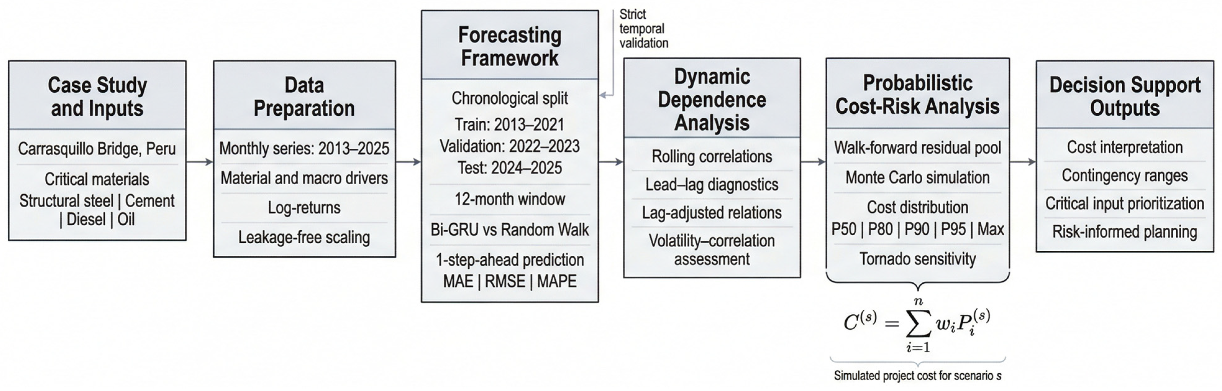
The workflow comprised five sequential stages, as shown in Figure 1. First, the case-study project was characterized, and the most cost-relevant construction inputs were identified from the bridge cost structure. Second, monthly time-series data for construction input indices and related macroeconomic drivers were compiled and preprocessed. Third, a comparative forecasting framework was implemented using a Bi-GRU model and a Random Walk benchmark under strict chronological partitioning. Fourth, dynamic dependence diagnostics were conducted through rolling correlations, lead–lag analysis, and a descriptive volatility–correlation assessment in order to identify time-varying co-movement patterns between oil and selected construction inputs. Fifth, the forecasting outputs were integrated into a Monte Carlo simulation scheme to estimate probabilistic cost-risk metrics, contingency levels at different percentiles, and the relative influence of key inputs on overall cost exposure.

This workflow was designed to connect time-series forecasting with project-level cost-risk interpretation in a case-based infrastructure setting. Such integration is consistent with recent construction management research emphasizing that forecasting tools become more useful when they support planning, control, and risk-informed decision-making rather than being assessed only through point-prediction accuracy [20,27,28].

2.2. Case Study, Variables, and Data Preparation

The empirical application focused on the Carrasquillo Bridge project in Peru. The selection of variables was guided by the cost structure of the case study and by the relevance of the inputs to bridge and road infrastructure projects. To clarify the scope of the case study,

Table 1. Case-study scope and material basket used in the probabilistic analysis.

Component	Description
Project type	Road infrastructure bridge project
Case-study location	Peru
Main analytical scope	Selected critical material basket
Included inputs	Structural steel, construction steel, cement, and diesel-related cost signals
Excluded inputs	Asphalt/bitumen and other materials not dominant in the selected bridge basket
Main cost-risk drivers	Construction steel and structural steel
Transferability condition	More applicable to bridge or road infrastructure components with steel-intensive cost structures
Main limitation for extrapolation	Not directly generalizable to road projects dominated by asphalt, earthworks, or pavement layers

summarizes the main characteristics of the selected bridge cost basket and the role of each input in the probabilistic analysis.

Accordingly, the findings are most transferable to road infrastructure components with steel-intensive material baskets and exposure to input price volatility. They should not be generalized without adjustment to projects in which asphalt, earthworks, pavement layers, or other cost components dominate the risk structure. The analysis considered the most influential construction inputs in the selected cost basket, including structural steel, construction steel, cement, and diesel-related cost signals, together with macroeconomic and external drivers such as oil, exchange rate, and CPI. This selection is consistent with the construction cost forecasting literature, which has shown that multivariate specifications provide a better representation of construction cost dynamics than purely univariate approaches when material prices are affected by broader economic conditions [7,8,10,24,29]. The construction input indices and the exchange rate and CPI series were obtained from [30]. The oil price series was obtained from [31]. The project quantities, unit prices, and material weights used to define the selected bridge cost basket were obtained from the case-study cost estimate. Further details on the input variables and the Monte Carlo cost basket are provided in Appendix B and Appendix C, respectively.

The dataset was organized as a strictly monthly level time series covering the period from January 2013 to December 2025. Because the variables were measured on different scales and the interest of the study was centered on temporal changes rather than absolute levels, the series were transformed into monthly log-returns before model estimation, as shown in (1). This transformation yielded an effective return series from February 2013 onward and supported the construction of 12-month input sequences for one-step-ahead forecasting. Log-return transformation is commonly used in time-series and price-dynamics studies because it improves comparability across variables and facilitates the analysis of relative variations over time [24,32]. Only strictly positive observations were retained in the original level series to preserve the validity of the logarithmic transformation.

$$r_{i,t}=\ln \left(X_{i,t}\right)-\ln \left(X_{i,t-1}\right)$$

(1)

where $ri:$ log-return of input i in period t and $Xi:$ index value or price of input i at time t. Therefore, the original level series were not used directly for model training; they were first transformed into monthly log-returns and later reconstructed into index levels for forecasting evaluation and cost simulation.

To preserve the temporal structure of the dataset and prevent information leakage, the forecasting design used a strict chronological split without shuffling. After constructing the 12-month input sequences, the target dates were divided into training (February 2014 to December 2021), validation (January 2022 to December 2023), and test (January 2024 to December 2025) subsets. This partitioning yielded 95 training samples, 24 validation samples, and 24 test samples. In addition, the scaling procedure was fitted only on the training log-return data and then applied unchanged to the validation and test subsets using a MinMaxScaler with range (−1, 1). This design follows best practices in forecasting evaluation, which recommend temporally ordered partitions, explicit benchmark comparison, and leakage-free preprocessing in order to obtain credible out-of-sample results [18,19]. This scaling was used only as a numerical preprocessing step for model estimation on log-returns; forecasting evaluation and cost simulation were conducted after reconstructing the series into index levels.

2.3. Comparative Forecasting Framework

The forecasting component was designed as a benchmark-aware comparative exercise. The main forecasting specification was a bidirectional gated recurrent unit (Bi-GRU) model. GRU architectures are frequently described as computationally lighter alternatives to LSTM because they require fewer parameters while retaining the ability to capture nonlinear temporal dependencies in sequential data [15,33,34]. This characteristic is particularly relevant for monthly construction-related time series of limited length, where parsimony and training stability are important considerations. Recent studies in construction and infrastructure forecasting have shown that GRU-based and hybrid recurrent architectures can achieve competitive performance in construction cost and highway cost-index prediction tasks [35].

The bidirectional structure was used to improve feature extraction within each historical input window. Importantly, the model did not use information beyond the forecast origin; rather, the sequence was processed in both directions only within the observed input window. The forecasting task was formulated as a one-step-ahead monthly prediction problem. The implementation adopted sliding windows, early stopping, and learning-rate reduction to limit overfitting and improve model generalization under a relatively short sample.

Therefore, the Bi-GRU model was not used under the assumption that deep learning would necessarily outperform simpler alternatives. Rather, it was included to test whether a recurrent multivariate architecture could provide practical gains over a transparent benchmark under a limited monthly dataset. The selected Bi-GRU configuration should be interpreted as a parsimonious and regularized recurrent specification for a short monthly dataset, rather than as the outcome of an exhaustive neural architecture search. The complete Bi-GRU model specification is provided in Appendix A.

The rationale for selecting Bi-GRU was that the forecasting task was formulated as a multivariate sequential problem, in which 12-month input windows combined four target input series with three exogenous variables. GRU-based architectures provide a recurrent structure for learning temporal dependencies while using fewer parameters than LSTM-based alternatives, which is relevant when the available monthly sample is limited [15,33,34]. However, given the small effective training size, the Bi-GRU specification should be interpreted as an exploratory recurrent benchmark rather than as a fully optimized deep learning architecture.

To place the performance of the Bi-GRU model in context, a Random Walk benchmark was also implemented. Benchmark comparison was considered essential because in persistent economic and price-index series, simple no-change forecasts often provide strong short-horizon performance and may be difficult to outperform consistently [18,19]. Accordingly, the objective of the comparison was not only to identify the model with the lowest forecasting error, but also to determine whether the additional complexity of a deep learning model yielded a meaningful practical gain over a transparent baseline.

More conventional machine learning methods, particularly tree-based models such as Random Forest, XGBoost, and related boosting approaches, may be more stable and competitive in small-sample settings when the problem is reformulated with lagged tabular features [12,13]. They were not included as additional benchmarks in this version because the objective was to evaluate the decision value of a recurrent multivariate specification against a transparent no-change benchmark, rather than to conduct an extensive model competition. Nevertheless, their inclusion is an important direction for future research.

The Random Walk benchmark was implemented as a univariate no-change forecast for each target input series. Therefore, it did not incorporate the exogenous variables used in the Bi-GRU specification. This choice is consistent with the role of Random Walk as a transparent benchmark. The benchmark was not intended to reproduce the same information set as the neural network, but to provide a transparent operational reference against which the practical value of the richer multivariate deep learning specification could be assessed. Consequently, the comparison should be interpreted as a benchmark-aware decision test rather than as a same-feature model competition.

Forecast accuracy was evaluated on reconstructed level series, since decision-making in construction budgeting and procurement is ultimately performed in the original cost-index space rather than in transformed returns. The evaluation relied on standard error metrics, including mean absolute error (MAE), root mean square error (RMSE), and mean absolute percentage error (MAPE), which are widely used in forecasting studies to compare predictive performance from complementary perspectives [18,19].

2.4. Dynamic Dependence Diagnostics

A lead–lag analysis was conducted by shifting the oil return series from 0 to 6 months in order to identify the lag associated with the maximum absolute correlation with the Cement_Index, Construction-Steel_Index, and Diesel_Index. This procedure was used to approximate the temporal association structure between oil and the selected construction-related price indices. The optimal lag for each target variable was then incorporated into a second rolling-correlation analysis to examine the time-varying behavior of the lag-adjusted relationships.

Additionally, rolling oil-price volatility was computed as the 12-month standard deviation of oil log-returns and descriptively contrasted with the lag-adjusted rolling correlations between oil and the selected construction input indices. Specifically, the analysis considered Structural-Steel_Index, Diesel_Index, Cement_Index, and Construction-Steel_Index, using in each case the optimal lag identified in the lead–lag assessment. This comparison was intended to examine whether periods of higher oil volatility tended to coincide with stronger or weaker time-varying co-movements across inputs. The volatility–correlation analysis was interpreted as a descriptive diagnostic rather than as a formal causal test.

2.5. Probabilistic Cost-Risk Simulation and Sensitivity Analysis

To translate the forecasting results and descriptive dependence diagnostics into project-level cost-risk evidence, a Monte Carlo simulation procedure was implemented. Recent construction research has shown that probabilistic modeling is particularly useful when material price volatility must be propagated into project-level cost risk, since point forecasts alone do not provide information on uncertainty ranges, percentile exposure, or contingency requirements [20,27,28]. Following this logic, the present study used simulated scenarios of critical input behavior to estimate the distribution of cost outcomes associated with the selected bridge cost basket.

For each simulation run, the project-level material cost was estimated by aggregating the simulated contribution of the selected critical inputs according to their participation in the case-study cost structure. In conceptual terms, the simulated cost outcome for scenario s can be expressed as shown in (2):

$${\mathrm{C}}^{\left(\mathrm{s}\right)}={\displaystyle \sum _{\mathrm{i}=1}^{\mathrm{n}}}{w}_i P_i^{\left(s\right)}$$

(2)

where w_i represents the relative participation of input i in the selected project cost basket, and Pi(s) denotes the simulated price level or cost factor of that input under scenario s. Repeated sampling produced an empirical distribution of possible cost outcomes for the selected bridge materials.

In the Monte Carlo stage, uncertainty was propagated from the forecasting layer to project-level cost outcomes by centering each simulation on the deterministic one-step-ahead return forecast for each material and period, and then adding stochastic shocks drawn from a model-specific walk-forward residual pool. For each forecasting model (Bi-GRU and Random Walk), 10,000 joint shock vectors were generated using a smoothed bootstrap procedure in which residual rows were resampled jointly across materials to preserve their empirical contemporaneous cross-dependence, and a small multivariate normal jitter based on the residual covariance matrix, estimated from the same model-specific walk-forward residual pool, was added to avoid repeated draws and smooth the simulated distribution. This procedure was intended to preserve empirical contemporaneous cross-dependence among residuals, but it was not designed as a formal nonlinear dependence or tail-dependence model. Also, in similar studies conducted in comparable contexts, a similar number of 10,000 iterations has also been used [22,23]. The simulated returns were then transformed into index levels using the previous observed month as the reconstruction base, after which index levels were converted into unit prices through proportional scaling relative to the selected cost base date and finally multiplied by material quantities to obtain simulated material costs and total project material cost. This design allowed forecast uncertainty to be translated explicitly into a probabilistic cost distribution while maintaining consistency with the observed cost structure of the case-study project.

The simulation results were summarized using central tendency and risk percentiles, particularly P50, P80, P90, and P95, together with maximum simulated exposure. These percentiles were used to quantify contingency requirements under different confidence levels, which is consistent with probabilistic cost-risk assessment practices in construction under material price uncertainty [20]. In this study, contingency was defined consistently as the difference between a target percentile of the simulated cost distribution and P50. Thus, the P90 and P95 contingencies correspond to P90 − P50 and P95 − P50, respectively.

In addition, a sensitivity analysis was performed to identify the relative importance of each input in the simulated cost distribution. The results were summarized through a tornado diagram, which provides a visual ranking of the dominant drivers of cost variability. This step was included because, from a project-management perspective, understanding which inputs contribute most strongly to overall uncertainty is essential for procurement review, monitoring priorities, and risk response planning [20,27].

3. Results

3.1. Comparative Forecasting Performance of Critical Construction Inputs

The forecasting stage was first assessed at the level of the individual input indices used in the project-level cost-risk framework.

Table 2. Forecasting performance of the Random Walk model on reconstructed input index levels.

Dataset	Material	MAE	RMSE	MAPE (%)
Validation	Structural-Steel_Index	21.4413	27.1682	2.600
Validation	Diesel_Index	37.8054	46.4328	3.294
Validation	Cement_Index	4.0992	6.0365	0.759
Validation	Construction-Steel_Index	25.2642	35.0949	2.858
Test	Structural-Steel_Index	17.7779	24.9534	2.135
Test	Diesel_Index	15.9500	20.2314	1.455
Test	Cement_Index	1.3725	2.7890	0.230
Test	Construction-Steel_Index	18.3867	25.8068	2.135

and

Table 3. Forecasting performance of the Bi-GRU model on reconstructed input index levels.

Dataset	Material	MAE	RMSE	MAPE (%)
Validation	Structural-Steel_Index	23.0491	28.1282	2.797
Validation	Diesel_Index	38.5893	47.7414	3.372
Validation	Cement_Index	4.4395	6.0649	0.822
Validation	Construction-Steel_Index	26.1018	35.6863	2.959
Test	Structural-Steel_Index	19.6047	26.4488	2.358
Test	Diesel_Index	14.7240	18.7658	1.338
Test	Cement_Index	1.7150	2.8211	0.286
Test	Construction-Steel_Index	20.1374	26.8024	2.351

summarize the one-step-ahead forecasting performance of the Random Walk and Bi-GRU models, respectively, on reconstructed level series for the validation and test subsets. This comparison is relevant because the subsequent probabilistic cost analysis depends on the quality of the underlying price projections.

Table 4. Relative RMSE variation with respect to the baseline model.

Dataset	Material	Relative RMSE Variation (%)
Validation	Structural-Steel_Index	3.53
Validation	Diesel_Index	2.82
Validation	Cement_Index	0.47
Validation	Construction-Steel_Index	1.69
Test	Structural-Steel_Index	5.99
Test	Diesel_Index	−7.24
Test	Cement_Index	1.15
Test	Construction-Steel_Index	3.86

complements this comparison by reporting the relative RMSE variation in Bi-GRU with respect to the Random Walk benchmark, thereby showing where model complexity translated into practical gains and where it did not.

The results indicate that the forecasting behavior was heterogeneous across materials. The Random Walk benchmark provided lower errors for most inputs and periods, confirming the persistence of several material price indices. However, the Bi-GRU model showed a relative advantage for diesel in the test period, suggesting that its nonlinear structure captured part of the short-term dynamics of this input more effectively than the benchmark. Cement exhibited the lowest forecasting errors under both models, whereas diesel and the steel-related indices showed larger deviations, particularly in the validation subset. These results indicate that forecasting gains were material-specific rather than uniform across the selected input basket.

Taken together, Table 2, Table 3 and Table 4 show that the benchmark remained competitive in most cases, while the Bi-GRU added value only selectively. This finding is important for the rest of the analysis because it suggests that model complexity should be judged not only by average forecasting performance, but also by whether it materially changes the project-level uncertainty envelope.

3.2. Lead–Lag Structure and Dynamic Dependence of Selected Inputs

The second stage of the results examined the temporal interaction between oil and the main construction inputs included in the selected bridge cost basket.

Table 5. Optimal lead–lag structure between oil and selected construction inputs.

Dependent Variable	Optimal Lag (Months)	Correlation *
Structural-Steel_Index	6	0.165
Diesel_Index	2	0.290
Cement_Index	5	0.205
Construction-Steel_Index	6	0.187

* These lag values should be interpreted as exploratory empirical monitoring horizons rather than as statistically validated lag structures or structural supply-chain delay estimates.

reports the optimal lead–lag structure obtained from the correlation analysis.

Because the estimated correlations are low to moderate, these results should be interpreted as descriptive association patterns rather than as evidence of causal price transmission.

Table 6. Volatility–correlation summary for lag-adjusted rolling relationships.

Window (Months)	Material	Lag Used (Months)	Series	Correlation
12	Structural-Steel_Index	6	Oil volatility vs. rolling Oil(t − 6)-Structural-Steel_Index(t) correlation	0.158
12	Diesel_Index	2	Oil volatility vs. rolling Oil(t − 2)-Diesel_Index(t) correlation	0.224
12	Cement_Index	5	Oil volatility vs. rolling Oil(t − 5)-Cement_Index(t) correlation	0.331
12	Construction-Steel_Index	6	Oil volatility vs. rolling Oil(t − 6)-Construction-Steel_Index(t) correlation	0.160

complements this analysis by presenting the descriptive association between rolling oil-price volatility and the lag-adjusted rolling correlation for each input. These results are relevant because they show whether the selected materials show associations with oil-related signals with similar timing or whether they exhibit differentiated co-movement patterns that may affect cost planning.

The lead–lag results indicate that diesel showed the strongest and most immediate association, while cement showed a delayed association and the steel-related indices reached their highest correlations at longer lags but with lower magnitude. This pattern suggests that the selected inputs did not exhibit synchronous associations with oil-related movements. The evidence from the lag-adjusted Oil–Cement series also shows that the relationship was regime-dependent rather than stable over time, with both sustained negative phases and one clearly sustained positive phase. Finally, the volatility–correlation assessment indicates that stronger oil volatility tended to coincide with stronger lag-adjusted co-movement, particularly for cement, although the strength of this association remained moderate.

These results indicate that the descriptive temporal relationships were both input-specific and time-varying. From a project-management perspective, this means that oil-related market signals should not be interpreted as affecting all inputs at the same horizon. Instead, procurement timing and contingency review may benefit from a differentiated view of how cement, diesel, and steel-related costs co-move with external market pressure over different horizons.

3.3. Probabilistic Cost-Risk Results from Monte Carlo Simulation

After forecasting the input indices and analyzing their dynamic interactions, the next stage translated the projected input behavior into project-level cost-risk metrics.

Table 7. Monte Carlo summary of total material cost by split and forecasting model.

Split	Model	P50 Total Cost (PEN)	P90 Total Cost (PEN)	P95 Total Cost (PEN)	Max Total Cost (PEN)	Contingency P90 − P50 (PEN)	Contingency P95 − P50 (PEN)
Test	Bi-GRU	84,880,373.91	88,460,274.81	89,631,531.28	96,784,156.50	3,579,900.90	4,751,157.37
Test	Random Walk	85,009,564.12	88,552,641.73	89,720,742.91	96,530,033.95	3,543,077.62	4,711,178.79
Validation	Bi-GRU	85,012,537.51	89,573,001.95	90,638,927.65	98,097,476.30	4,560,464.44	5,626,390.14
Validation	Random Walk	85,318,620.45	89,855,126.17	90,916,549.69	97,966,338.55	4,536,505.72	5,597,929.24

summarizes the Monte Carlo results for the validation and test subsets under both forecasting models. This table is relevant because it moves the analysis from individual input forecasts toward the distribution of total material cost for the selected bridge cost basket. In addition to P50, P90, P95, and maximum simulated values, the table reports percentile-based contingencies measured as the difference between the upper percentile and P50.

The simulation results show that the uncertainty band was wider in validation than in test under both forecasting models, which is consistent with the larger forecast errors observed in the validation subset. At the aggregate cost level, both models produced very similar central and upper-tail values, suggesting that the project-level probabilistic envelope was relatively robust to the forecasting specification. In the test subset, the Random Walk model generated slightly higher central and upper percentile estimates, while the Bi-GRU model produced a slightly higher maximum simulated exposure. Thus, the main difference between models was not the central range of the distribution, but the behavior of the extreme right tail.

To provide a more detailed view of the latest test period,

Table 8. Probabilistic cost results for the latest test period (December 2025).

Period	Model	Deterministic Total Cost (PEN)	P50 Total Cost (PEN)	P90 Total Cost (PEN)	P95 Total Cost (PEN)	Max Total Cost (PEN)	Contingency P90 − P50 (PEN)	Contingency P95 − P50 (PEN)
December 2025	Bi-GRU	80,767,416.01	81,384,837.56	83,654,970.36	84,478,312.01	87,733,194.61	2,270,132.80	3,093,474.46
December 2025	Random Walk	80,684,156.78	81,466,666.54	83,665,782.33	84,616,037.63	88,667,436.71	2,199,115.80	3,149,371.09

reports the deterministic total cost, and simulated percentile outcomes for December 2025. This table is relevant because it translates the model outputs into a single decision point that can be interpreted directly in budgeting and contingency terms. In both models, the deterministic estimate remained very close to the observed total cost, while the probabilistic percentiles shifted the expected exposure upward. The two models again yielded highly similar central values, although the Random Walk specification produced a slightly wider extreme tail in the latest period.

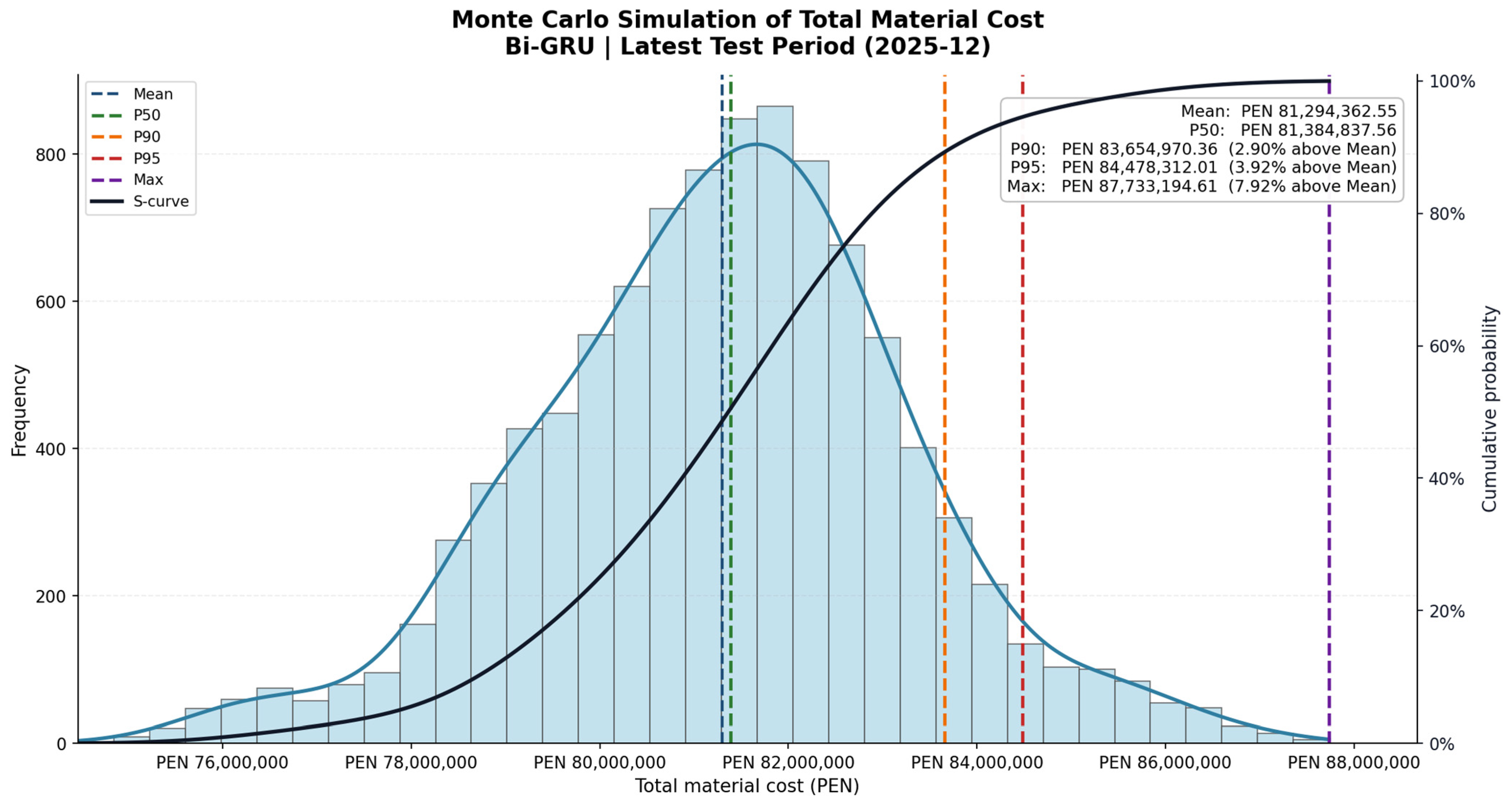
The maximum simulated value should be interpreted only as an exploratory extreme-tail indicator, since it is sensitive to the number of simulations and distributional assumptions. For contingency estimation, the main decision indicators in this study are P90 and P95. Figure 2 shows that the Bi-GRU-based distribution is centered slightly above the observed cost and exhibits a moderate right tail. The mean and P50 are close to each other, indicating that the simulated distribution remains reasonably concentrated in its central range. The separation between P50, P90, and P95 is visible but controlled, which suggests a moderate upward risk band for the latest test period. The maximum simulated value lies notably farther to the right, indicating that extreme upside cost outcomes remain possible even though they are located in the low-probability tail.

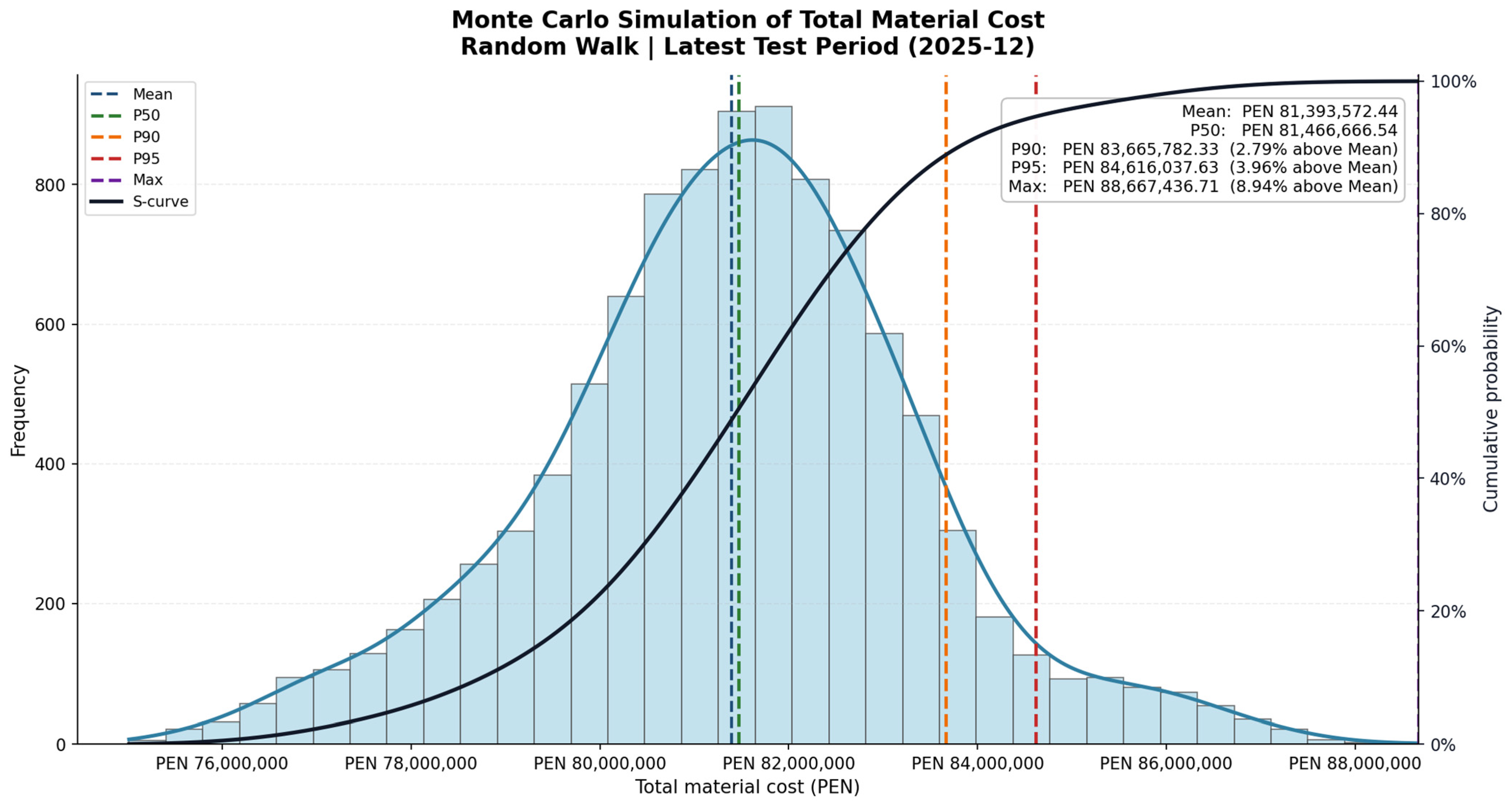
Figure 3 presents a very similar central pattern for the Random Walk-based simulation, confirming that both forecasting models generate comparable median and upper-percentile cost levels. However, the right tail extends further than in the Bi-GRU case, and the maximum simulated value is higher. This suggests that the Random Walk specification preserves a slightly heavier extreme-cost tail in the latest period, even though its central percentile estimates remain close to those obtained under Bi-GRU.

Taken together, Table 7 and Figure 2 and Figure 3 show that the probabilistic interpretation is more informative than the deterministic estimate alone. Although the deterministic totals nearly match the observed cost, the simulation reveals a non-negligible contingency requirement if the decision-maker wishes to operate at P90 or P95 confidence levels. In practical terms, the latest-period results indicate that the additional cost allowance required to move from the central estimate to a higher-confidence estimate is material and should not be ignored in cost planning.

3.4. Sensitivity of Total Cost to Critical Inputs

The final stage of the results assessed which inputs most strongly influenced the simulated total material cost.

Table 9. Sensitivity ranking of critical inputs in the latest test-period simulation.

Model	Material	Spearman Correlation with Total Cost	Absolute Spearman
Bi-GRU	Cement_Index	0.2992	0.2992
Bi-GRU	Diesel_Index	0.5439	0.5439
Bi-GRU	Structural-Steel_Index	0.7909	0.7909
Bi-GRU	Construction-Steel_Index	0.9015	0.9015
Random Walk	Cement_Index	0.2265	0.2265
Random Walk	Diesel_Index	0.5494	0.5494
Random Walk	Structural-Steel_Index *	0.8140	0.8140
Random Walk	Construction-Steel_Index *	0.8945	0.8945

* The dominance of steel-related inputs reflects the combined effect of their cost participation in the selected bridge basket and their simulated price variability. Therefore, their influence should not be interpreted as a volatility effect alone.

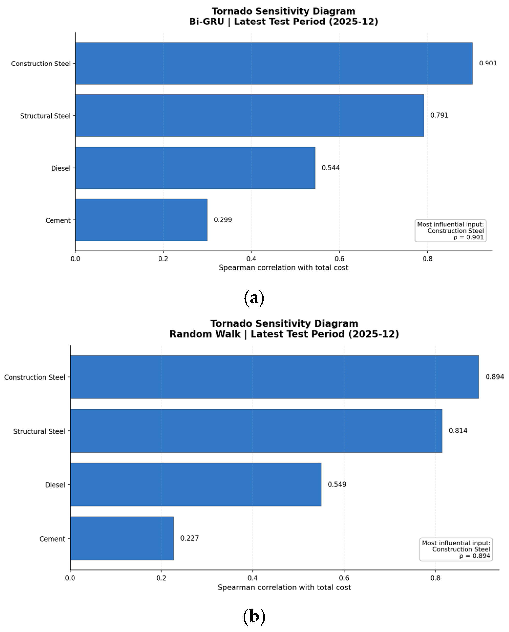
demonstrates the Spearman correlations between each input and total cost for the latest test-period simulation under both forecasting models. This table is relevant because it ranks the dominant drivers of uncertainty within the bridge material basket and therefore supports prioritization in procurement monitoring and contingency management. Figure 4 complements this evidence by presenting the tornado sensitivity diagrams for both models in a single two-panel figure.

The sensitivity results are highly consistent across the two forecasting specifications. In both cases, Construction Steel was the most influential driver of total cost variability, followed by Structural Steel. Diesel showed a moderate contribution, whereas Cement exhibited the weakest sensitivity. This ranking indicates that steel-related items dominated the propagation of cost uncertainty in the selected bridge basket. However, this does not imply that the remaining inputs should be ignored. Rather, it indicates that marginal forecast errors or price shocks in steel-related inputs are more likely to shift the contingency envelope than comparable disturbances in less influential materials such as cement. The stability of this ordering across both models strengthens the managerial relevance of the result, since the prioritization of key inputs does not depend materially on the selected forecasting approach.

Figure 4 confirms the dominance of steel-related inputs in the simulated cost-risk structure. In panel (a), corresponding to the Bi-GRU simulation, Construction Steel exhibits the highest association with total cost, followed by Structural Steel, while Diesel and Cement have clearly smaller effects. Panel (b), corresponding to the Random Walk simulation, shows the same ranking with only marginal differences in magnitude. The visual agreement between both panels indicates that the principal cost-risk drivers are structurally stable and not an artifact of a specific forecasting model. From an engineering standpoint, this means that risk monitoring and contingency review should focus first on steel-related inputs, with diesel as a secondary driver and cement as a comparatively less influential contributor to the variability of the selected material basket.

Results show that the Random Walk benchmark remained competitive at the forecasting stage, that the dynamic dependence structure among oil and the selected inputs was heterogeneous and lag-sensitive, and that the project-level probabilistic cost envelope was driven primarily by steel-related inputs. The Monte Carlo framework further showed that, even when deterministic totals remain close to observed costs, the upper-tail exposure and contingency requirements can still be material for engineering decision-making.

4. Discussion

Rather than proposing a new dependence model, this study provides case-based empirical evidence on how comparative forecasting and probabilistic simulation can support contingency-oriented cost interpretation in bridge infrastructure under input price volatility.

4.1. Analysis of Forecasting Performance and Cost-Risk Implications

Within the two-model comparison conducted in this case study, the Random Walk benchmark provided the stronger forecasting reference for most inputs. The model achieved lower forecasting errors for most inputs and, in the latest-period simulation, produced a slightly wider extreme right tail than Bi-GRU. This combination is relevant for engineering practice because the decision depends not only on average fit, but also on the model’s ability to represent low-frequency, high-impact cost overrun scenarios.

The superior performance of the Random Walk benchmark in most comparisons may be explained by the persistence and noise observed in monthly construction input price indices. At short horizons, the latest observed value may provide a stronger signal than complex nonlinear patterns, especially under abrupt and non-stationary market shocks. Although Bi-GRU incorporated a richer 12-month multivariate structure, the limited training sample likely reduced its capacity to learn stable relationships between exogenous variables and material prices. Thus, the finding does not weaken the forecasting–simulation framework; rather, it shows that model complexity does not necessarily improve cost-risk information under persistent, noisy, and short-horizon conditions. This behavior is consistent with near-random-walk dynamics at the monthly forecasting horizon, where persistence and short-term noise may dominate over learnable nonlinear structure.

The simulation confirms that both models produced similar central and upper-percentile values. Expressed relative to the selected central reference, the Bi-GRU model produced increases of 2.90% at P90 and 3.92% at P95, while the Random Walk model produced 2.79% and 3.96%, respectively. Therefore, the main decision indicators remain P90 and P95. Maximum simulated values were retained only as exploratory extreme-tail references and were not used to define contingency levels.

The sensitivity diagrams reinforce this interpretation. In Bi-GRU, construction steel reached a 90.1% correlation with total cost, followed by structural steel with 79.1%, diesel with 54.4%, and cement with 29.9%. In Random Walk, the values were 89.4%, 81.4%, 54.9%, and 22.7%, respectively. Both models preserve the same ranking of importance. Therefore, the study clearly identifies that total cost variability is concentrated in steel-related inputs, while cement contributes a significantly smaller effect.

The results also suggest that the additional exogenous information used by the Bi-GRU did not consistently improve out-of-sample accuracy. This may indicate that the oil, exchange-rate, and CPI signals were either weakly associated, temporally unstable, or difficult to learn reliably from the available sample size.

This evidence has direct implications for practice. The project should not distribute contingency uniformly across materials. Management should focus market monitoring, price review, procurement strategy, and contractual discussion on construction steel and structural steel.

4.2. Comparison with the Relevant Literature

The results are consistent with the forecasting literature, which cautions against assuming the superiority of complex models over benchmark statistical approaches a priori. Makridakis et al. argue that machine learning methods do not necessarily outperform traditional approaches, particularly in highly persistent time series [18]. Similarly, Hewamalage et al. emphasize the importance of benchmarking against reference models and applying rigorous temporal validation schemes in forecasting studies [19]. The present study follows this approach by explicitly comparing Bi-GRU and Random Walk under a chronological evaluation framework, allowing the results to be interpreted within a robust methodological context. In this setting, the findings confirm that greater model complexity does not automatically translate into better performance for decision-making.

However, artificial intelligence and deep learning models remain valuable tools for cost engineering. Previous research has shown that models such as GRU, LSTM, and their hybrid variants can achieve strong performance in forecasting construction costs and indices [35,36,37]. Nevertheless, these studies also highlight that performance depends on data structure, forecasting horizon, and evaluation design. In the present case study, the deep learning model demonstrates competitive performance but does not surpass the benchmark statistical model as the preferred alternative for decision-making in a contingency analysis context.

The behavior of construction inputs is also aligned with the literature on dynamic relationships between energy and material prices. Several studies have documented time-varying dependencies and lag structures between oil and metal markets, as well as associations that vary across economic regimes [38]. The results of this study follow this pattern, showing that cost variability is not evenly distributed across inputs and that the association with external shocks differs according to the specific material considered.

The sensitivity analysis is consistent with empirical evidence in construction economics. Previous studies have shown that material inflation and macroeconomic variables affect cost components differently, with inputs characterized by higher energy intensity and logistical exposure concentrating a larger share of risk [25,39]. In this study, the predominance of steel-related inputs as the main drivers of cost variability is consistent with this literature and with the technical nature of infrastructure projects such as bridges.

4.3. Implications for Engineering Decision-Making in Construction Projects

From a cost management perspective, contingency should be defined as a budgetary decision based on confidence levels rather than as a fixed add-on. The results show that the contingency at the P95 level can reach 3.96%, while the maximum simulated exposure is reported only as an exploratory extreme-tail reference. Despite this, each project must estimate its own contingency, as there is no fixed range for its calculation.

The P95 contingency of approximately 4% should not be interpreted as evidence that conventional 5–10% buffers are necessarily excessive. The result is specific to the selected bridge material basket, the modeled inputs, and the observed price conditions of the case study. Therefore, it should be understood as a project-specific probabilistic estimate rather than as a general replacement for standard contingency ranges. It is important to clarify that the contingency percentages reported in this study are calculated with respect to the simulated cost distribution of the selected bridge material basket. They do not represent a contingency applied to the entire contract budget or a general emergency reserve for the whole project. Therefore, comparisons with contingency ranges reported in other infrastructure studies should be interpreted as contextual benchmarks rather than as strictly equivalent calculation bases.

Other studies, such as one in water infrastructure, reported that a contingency of 8.46% was added but 13.58% was required, while another study in hydropower projects found contingency ranges between 8.28% and 17.97% [4]. The values obtained in this study are generally consistent with those reported in the literature; however, it is important to emphasize that each project should independently determine its contingency. Previous research in road infrastructure has reported contingency ranges between 1.34% and 11% [22]. Moreover, the results of this study complement previous stochastic applications by linking comparative forecasting outputs and residual-based simulation to probabilistic contingency estimation under input price volatility [23]. Consequently, infrastructure budgeting should link contingency reserves to explicit confidence targets and actual risk conditions, rather than to historically comfortable percentages. In this case study, the longer empirical association horizon observed for steel-related inputs suggests that procurement reviews and contingency updates should not be limited to immediate price movements but should also consider delayed co-movement windows when evaluating steel-intensive packages.

4.4. Limitations and Future Research

This study has two main limitations. First, the analysis relies on a relatively short monthly sample and on aggregated indices, which restricts the granularity of project-level decision rules. After constructing 12-month input sequences, the Bi-GRU model was trained with only 95 samples. This small effective training size increases the risk of overfitting and limits the reliability, stability, and generalizability of the neural-network results. Although early stopping, dropout, learning-rate reduction, and chronological validation were used to reduce this risk, no repeated-run analysis, random-seed sensitivity test, or exhaustive hyperparameter search was conducted. Therefore, the Bi-GRU results should be interpreted as indicative evidence for this case-study dataset rather than as a definitive validation of the architecture or as evidence of a stable architecture-level advantage.

Although this level of aggregation is useful for identifying broad cost-risk patterns, it does not fully capture the heterogeneity that may exist across specific materials, suppliers, procurement packages, or contract items. As a result, the practical translation of the results into detailed operational rules for purchasing, escalation clauses, or contingency release remains limited.

Second, the dynamic analysis adopted in this study is descriptive and does not establish formal causal transmission mechanisms among oil, macroeconomic drivers, and construction materials. The rolling correlations, lag diagnostics, and volatility-based comparisons are useful for identifying temporal patterns and possible association structures, but they do not provide a structural explanation of how shocks are associated across markets. Therefore, the results should be interpreted as decision-support evidence rather than as causal proof of market behavior. A related limitation is that the residual-based simulation does not explicitly test nonlinear dependence or alternative tail-dependence structures.

These limitations suggest several methodological recommendations for future research. A first recommendation is to test more formal time-varying dependence models capable of representing changing interaction structures across market regimes. In that regard, copula-based approaches [40,41] offer a promising extension because they allow the analyst to move beyond linear correlation and to represent asymmetric and upper-tail dependence more explicitly. Future studies could therefore compare Gaussian, Student-t, and Archimedean copulas, as well as dynamic copula specifications, to examine whether tail behavior changes over time and whether contingency estimates remain stable under alternative dependence assumptions.

A second recommendation concerns the forecasting component. Although the present study used Bi-GRU as the deep learning specification, the literature has shown that LSTM-based models remain one of the most robust alternatives for modeling nonlinear temporal dynamics in construction cost indices and related infrastructure signals. For that reason, future research should evaluate whether LSTM or hybrid LSTM-based architectures provide a better balance between predictive accuracy, temporal stability, and downstream risk simulation performance [35,36,42]. This recommendation does not imply that the current modeling choice was inappropriate, but rather that LSTM deserves explicit examination as a complementary benchmark within the same forecasting-plus-simulation framework.

A third recommendation is to strengthen the treatment of exogenous variables. Construction material prices are not driven only by their own past behavior, but also by fuel prices, exchange rates, inflation, and other macroeconomic signals [26]. In addition, the exogenous variable set was limited to oil, exchange rate, and CPI. Other macroeconomic, political, and logistics-related factors, such as local political stability, international freight conditions, or global logistics indices, may also affect construction material prices in emerging markets and should be considered in future extensions.

Future studies should compare recurrent neural architectures with conventional machine learning models such as Random Forest, XGBoost, and LightGBM using lagged-feature formulations, repeated temporal validation, and random-seed sensitivity analysis, particularly in small or moderate construction cost datasets. They should also extend the benchmark set to include classical time-series models such as ARIMA/ARIMAX, VAR/VECM, and exponential smoothing, particularly when the objective is to compare forecasting suitability rather than to test the decision value of a transparent baseline.

5. Conclusions

This study examined how construction input price forecasting, descriptive temporal diagnostics, and Monte Carlo simulation can inform probabilistic contingency estimation in a road infrastructure case study, using the Carrasquillo Bridge in Peru as the empirical application. The framework combined benchmark-aware forecasting, dynamic dependence diagnostics, Monte Carlo simulation, and sensitivity analysis to evaluate how critical construction input prices affect project-level contingency requirements.

Among the two tested models, the Random Walk benchmark provided lower forecasting errors for most inputs in the case-study dataset. Although the Bi-GRU model achieved competitive performance, it did not consistently outperform the statistical benchmark. Random Walk provided lower forecasting errors for most inputs and preserved a more severe upper tail in the simulated cost distribution, which is especially relevant for contingency-oriented decision-making.

The dynamic analysis also showed that the relationship between oil and the selected inputs was heterogeneous and time-varying. Diesel exhibited the strongest short-term association, cement showed a delayed association, and steel-related inputs presented differentiated lag structures. These findings indicate that cost-related associations do not occur uniformly across materials and that contingency review should consider material-specific timing.

At the project level, the Monte Carlo results confirmed that both models produced similar central estimates but differed more clearly in the upper tail. The P95 contingency reached 3.92% under Bi-GRU and 3.96% under Random Walk, confirming that both forecasting specifications produced similar upper-percentile contingency estimates. These results support the interpretation of contingency as a confidence-based budgeting decision rather than as a fixed percentage in projects exposed to construction input price volatility. The sensitivity analysis further identified construction steel and structural steel as the main drivers of total material-cost variability.

Beyond these empirical results, the study contributes to construction cost-risk management in three ways. First, it provides an integrated forecasting–simulation workflow that converts construction input price uncertainty into percentile-based contingency information for project-level decision-making. Second, it shows that benchmark models should not be treated merely as secondary comparators, since a transparent Random Walk specification may provide more robust decision support than a more complex neural architecture when price indices are persistent and the available sample is limited. Third, it translates probabilistic outputs into managerial priorities by identifying which inputs dominate the simulated cost-risk envelope. These contributions reinforce the need to define contingency as a confidence-based, project-specific decision rather than as a fixed percentage applied uniformly across infrastructure projects.