Time-Domain Feature-Based Anomaly Detection of Extreme Vibration Events for Cross-River Bridge Piers

Abstract

This study proposes a time-domain feature-based anomaly detection method for vibration data of bridge piers collected by underwater seismometers operating under alternating submerged and exposed conditions. The method aims to accurately identify anomalies under both normal and extreme events. Taking the Fuzhou Pushang Bridge as a case study, the acceleration root mean square (a_RMS) is adopted as the representative vibration feature to investigate the effects of vehicular loads, water level variations, and tidal fluctuations. The results show that pier vibrations are primarily dominated by vehicular loads, exhibiting pronounced daily periodicity, intraday non-stationarity, and non-normality, while the influences of water level and tidal variations are relatively minor. Based on these characteristics, an anomaly detection framework integrating STL decomposition (Seasonal-trend decomposition using Loess), Yeo–Johnson transformation, and control charts is developed. Historical data are used to establish control limits and conduct self-validation, yielding an anomaly rate of 0.14%, which is consistent with the theoretical probability of ±3σ control limits. When applied to the subsequent monitoring period, the anomaly rate under normal conditions is 0.18%, demonstrating the stability of the proposed method. Further analysis reveals that anomalies are primarily caused by direct hydrodynamic impacts on the instrument. Under flood conditions, continuous anomalies occur during nighttime, with the anomaly rate increasing to 4.44%. Under seismic conditions, the control chart statistic reaches 5.03, significantly exceeding the control limits. Comparative analysis shows that the percentile-based method yields a higher anomaly rate (0.65%), indicating a higher false alarm rate. Overall, the proposed method demonstrates strong generalization capability and reliability, providing effective support for long-term structural health monitoring of bridge substructures in complex environments.

1. Introduction

Nowadays, structural health monitoring (SHM) has been widely applied in civil and mechanical engineering and has become an important approach for ensuring the full life-cycle safety management of bridges [1,2,3,4]. In recent years, many representative long-span bridges, such as the Tsing Ma Bridge [5], the Hong Kong–Zhuhai–Macao Bridge [6], and the Akashi Kaikyo Bridge [7], have implemented SHM systems, providing essential support for operation management, maintenance decision-making, and safety assessment [8]. A typical SHM system consists of several components, including sensor deployment, data acquisition, data transmission, structural damage detection, and alarm generation. Among these, sensor deployment serves as the foundation, continuously capturing structural responses and external loads, thereby providing reliable data for structural condition assessment [9].

However, due to the harsh underwater working environment of sensors, existing SHM systems primarily focus on superstructures such as girders, decks, and towers [10,11,12]. In contrast, long-term monitoring of substructures remains limited, and a systematic and reliable monitoring framework for bridge substructures has yet to be fully established. For long-span bridges crossing rivers or estuaries, substructures such as piers and piles are continuously exposed to harsh environmental conditions, including hydraulic scour, saline corrosion, and material degradation. These factors inevitably lead to damage accumulation and a reduction in load-bearing capacity over time [13]. According to the Federal Highway Administration (FHWA), there are 26,727 bridges in the United States over waterways or in tidal zones with unknown foundation conditions, highlighting the critical importance of substructure safety [14]. Therefore, there is an urgent need to develop effective monitoring technologies for bridge substructures to enable real-time perception, dynamic assessment, and early warning of structural safety.

In this context, an improved ocean bottom seismometer (OBS), hereafter referred to as an underwater seismometer, is adopted in this study for long-term vibration monitoring of bridge piers. Originally developed in the 1960s for underwater nuclear test detection [15], OBS technology has evolved substantially with advances in sensing, data acquisition, and communication technologies. It has been widely applied in seafloor seismic observation [16], marine geophysical exploration [17], hydrocarbon surveys [18], and other marine applications [19]. However, when deployed in underwater environments, seismometers are inevitably subjected to hydrodynamic disturbances, instrument aging, and communication instability, all of which may introduce significant noise and abnormal measurements. If such anomalies are not properly identified and removed, they may lead to false alarms and compromise the reliability of structural condition assessment results. Therefore, robust anomaly detection is a prerequisite for ensuring the accuracy and reliability of subsequent structural evaluation [20].

Currently, a large body of literature has reported methods for anomaly detection in monitoring data, which can be broadly classified into three categories: probabilistic statistical methods [21], predictive models [22], and computer vision approaches [23]. Among these approaches, artificial intelligence-based deep learning techniques are mainly applied in predictive models and image-based methods and have gradually become the dominant implementation paradigm [24,25,26]. Such methods construct deep neural network architectures to automatically extract nonlinear features from complex monitoring data, thereby enabling effective identification of anomalous patterns. In contrast, probabilistic statistical methods represent a lightweight technical approach. Their fundamental assumption is that normal data points tend to cluster closely in the feature space, whereas anomalous data deviate significantly from this distribution. Accordingly, statistical models and thresholds can be established using historical monitoring data, and observations exceeding predefined thresholds are identified as anomalies. These methods are characterized by clear physical interpretation, simple implementation, and ease of use. In practical applications, a key challenge in statistical-based anomaly detection lies in mitigating the influence of environmental factors (such as temperature and loading conditions) on monitoring data so as to develop reliable and robust statistical models [27,28,29]. However, research on the influence of environmental effects on bridge pier vibration responses remains relatively limited, and there is still a lack of stable statistical models and anomaly detection methods suitable for complex hydrodynamic environments.

In this study, long-term monitoring data from underwater seismometers installed on the Fuzhou Pushang Bridge are analyzed. The a_RMS is used to characterize vibration intensity, and the effects of vehicular loads, water level variations, and tidal fluctuations are systematically investigated. On this basis, a time-domain anomaly detection framework is proposed. The method employs STL decomposition to separate trend and periodic components, applies the Yeo–Johnson transformation to address non-normality, and utilizes control charts to identify anomalies. The effectiveness and reliability of the proposed method are validated through a case study based on long-term monitoring data and comparison with a conventional percentile-based approach.

2. Characteristics of Monitoring Data and Influencing Factors

2.1. Monitoring System and Data Description

2.1.1. Bridge and Monitoring System Setup

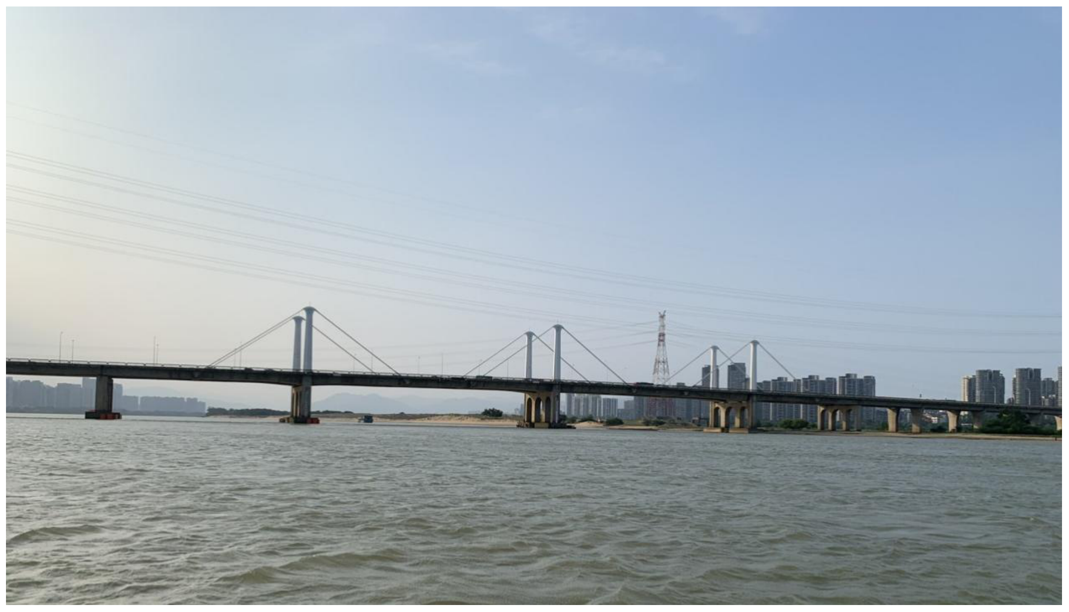
The Fuzhou Pushang Bridge (as shown in Figure 1) is a cross-river bridge in China, connecting Minhou County in the west to Cangshan District in the east. Completed in 2007, the bridge has a total length of 1464 m and consists of three segments: an eastern non-navigable span, a central navigable span, and a western non-navigable span. The eastern segment is a 750 m prestressed concrete continuous girder bridge consisting of three units, each with five 50 m spans. The central navigation span adopts a cable-stayed structure with a single cable plane and a symmetric layout of 72 m + 110 m + 110 m + 72 m. The western segment is a 350 m prestressed concrete continuous girder bridge, comprising two continuous units: the first with four 50 m spans and the second with three 50 m spans. According to field measurements, the fundamental frequency of the bridge is 1.04 Hz.

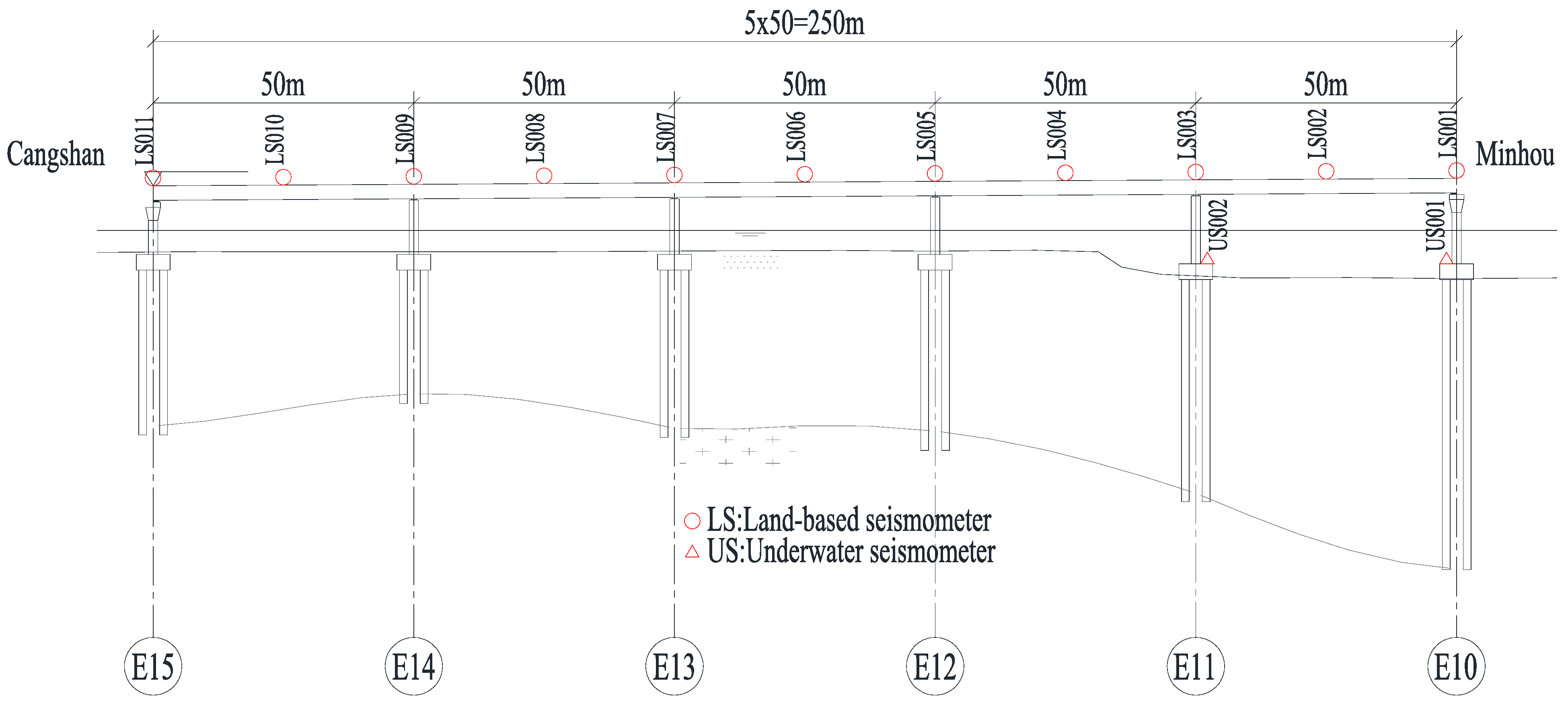
A full-bridge vibration monitoring system (as shown in Figure 2) was deployed to enable real-time monitoring of both superstructure and substructure responses. Eleven seismometers were installed at the bridge bearings and mid-spans, while two underwater seismometers were positioned on the pile caps (E10 and E11) located in the river. The underwater seismometer is based on a split-type OBS developed by the Southern University of Science and Technology [15], whose core sensing component is the Trillium Compact 120 s broadband seismometer manufactured by Nanometrics, Canada. Detailed technical specifications are listed in

Table 1. Technical specifications of the seismometer.

Index	Seismometer	Underwater Seismometer
Bandwidth	60 s–100 Hz	120 s–100 Hz
Sensitivity	2000 V·s/m	750 V·s/m
Sampling frequency	100 Hz	100 Hz
Leveling method	Auto-leveling	Auto-leveling

. Each measurement point records vibration responses in three orthogonal directions (transverse, longitudinal, and vertical), providing velocity time histories for subsequent analysis.

2.1.2. Data Acquisition

In this study, monitoring data from the underwater seismometer installed at pier E11 were selected for analysis. The seismometer has been continuously recording since June 2023, and a one-year dataset (June 2023 to June 2024) was used for systematic investigation. During this period, two seismic events and one flood event were identified. The corresponding earthquake parameters are summarized in

Table 2. Earthquake parameters.

No.	Epicenter Location	Origin Time (UTC + 8)	Focal Depth (km)	Magnitude (M)	Epicentral Distance (km)
1	Offshore Hualien County, Taiwan, China	2024-04-03 07:58:08	12	7.3	345.13
2	Offshore Hualien County, Taiwan, China	2024-08-16 07:35:52	16	6.3	374.59

.

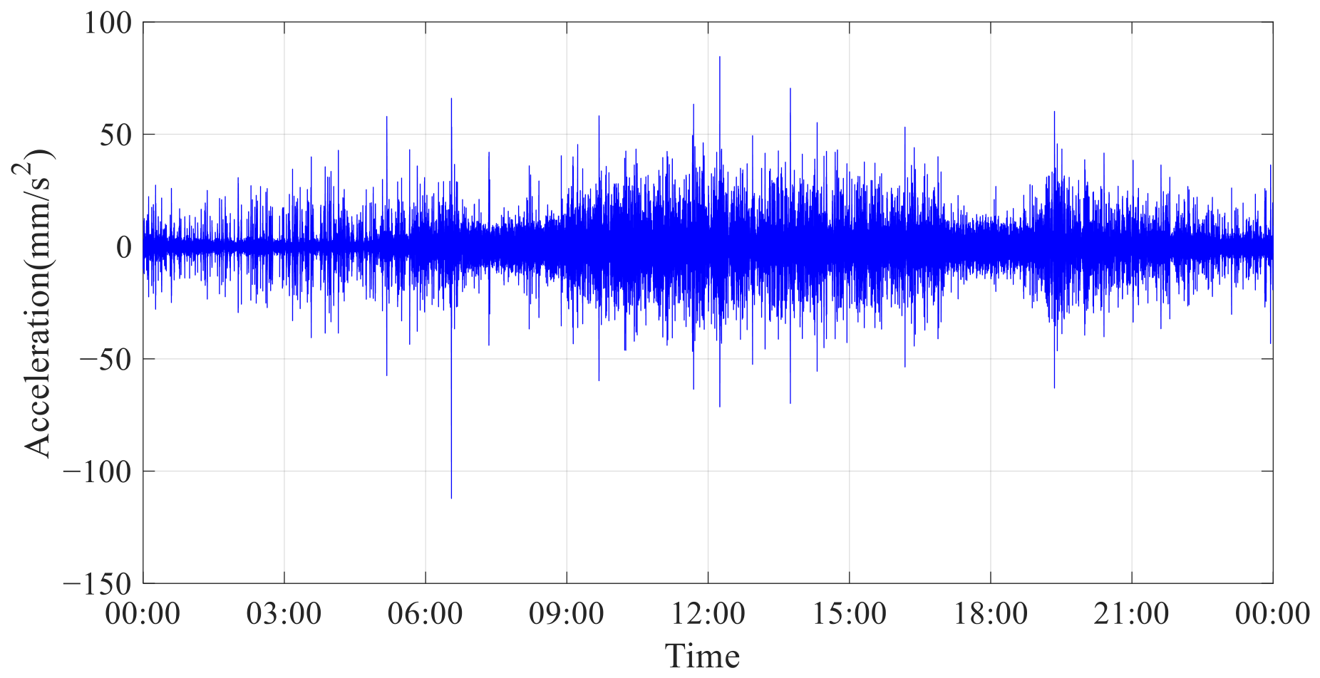
The a_RMS was adopted as the primary indicator to characterize vibration intensity. It is defined as the root mean square value of the acceleration time history and is used to represent the overall energy level of the vibration response. Velocity records were first converted into acceleration time histories through instrument response removal, detrending (mean and linear trend removal), and numerical differentiation (as shown in Figure 3). To balance sensitivity to transient events and statistical stability, and following empirical guidelines for seismic observation window lengths [30,31], the window length was selected to cover both several complete structural vibration cycles and the duration of vehicle passage (typically 5–10 s). Accordingly, a window length of 60 s was adopted in this study.

2.2. Environmental and Operational Factors

Under normal conditions, the vibration response of bridge piers is influenced by multiple environmental and operational factors, including vehicular loads, water level variations, and tidal fluctuations. To establish a reliable anomaly detection model, it is necessary to quantify the influence of these factors.

2.2.1. Vehicular Loads

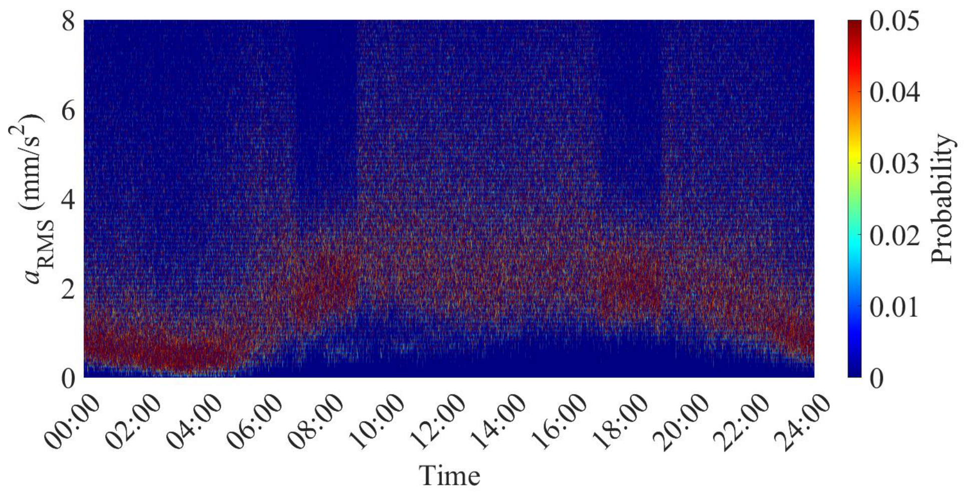
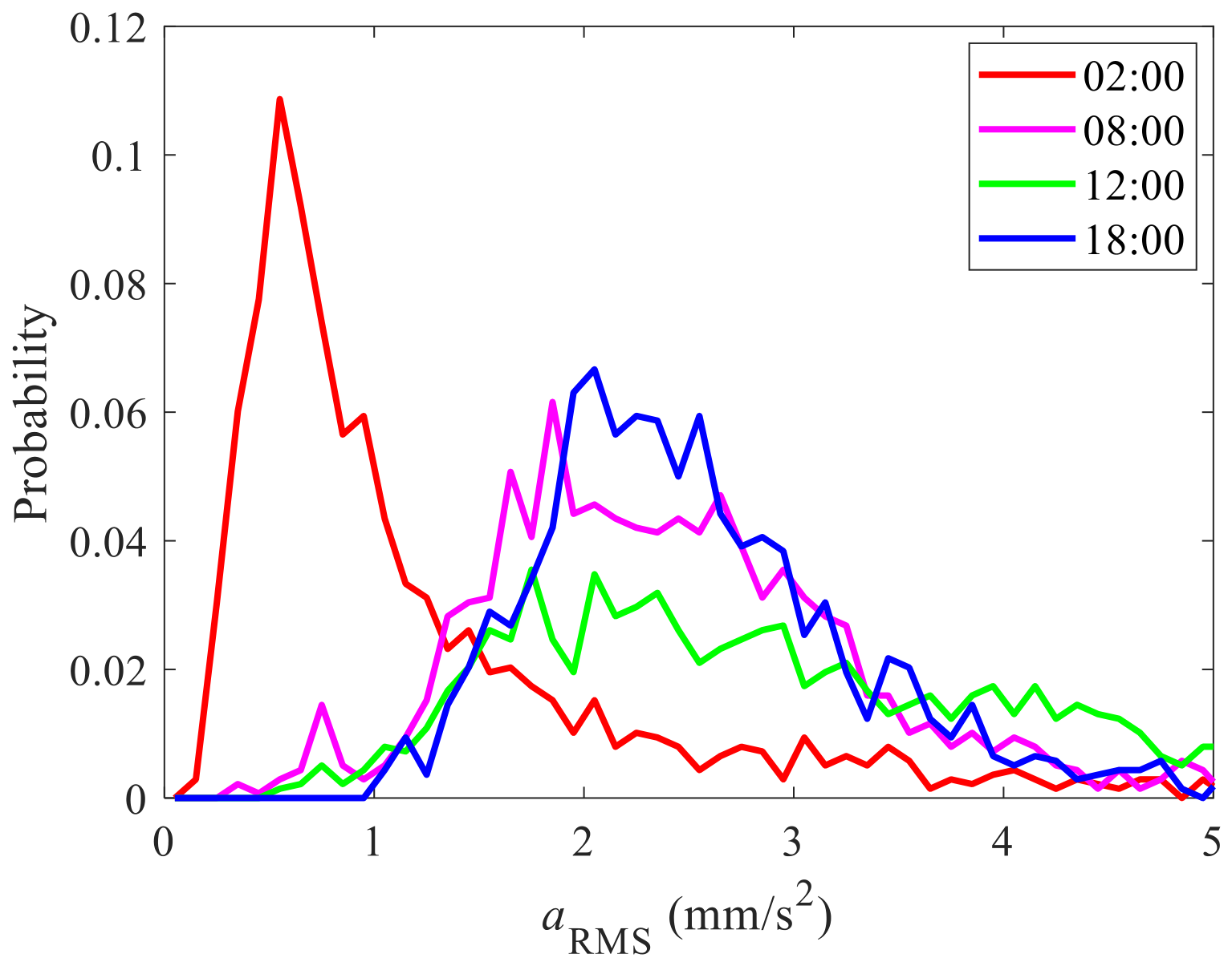
To minimize the influence of abnormal traffic conditions during holidays, a continuous one-month dataset collected in July was selected. Due to the daily periodicity of traffic flow, the probability distribution of a_RMS was calculated at the same time across different days (as illustrated in Figure 4). Given the high consistency of vibration characteristics among the three directions, only the transverse results are presented, while the longitudinal and vertical responses are omitted for brevity. The results indicate a strong correlation between a_RMS and traffic patterns. Based on traffic characteristics, a 24 h day was divided into four periods: morning peak (07:00–09:00), evening peak (17:00–19:00), off-peak daytime (05:00–23:00, excluding peak periods), and nighttime (23:00–05:00). For each period, a representative 1 h segment of a_RMS data was selected for probability distribution analysis, as shown in Figure 5. The results show that the amplitudes and variability of a_RMS during the morning and evening peak periods were slightly lower than those during the off-peak period, whereas the amplitudes and variability during nighttime were significantly reduced compared to daytime conditions.

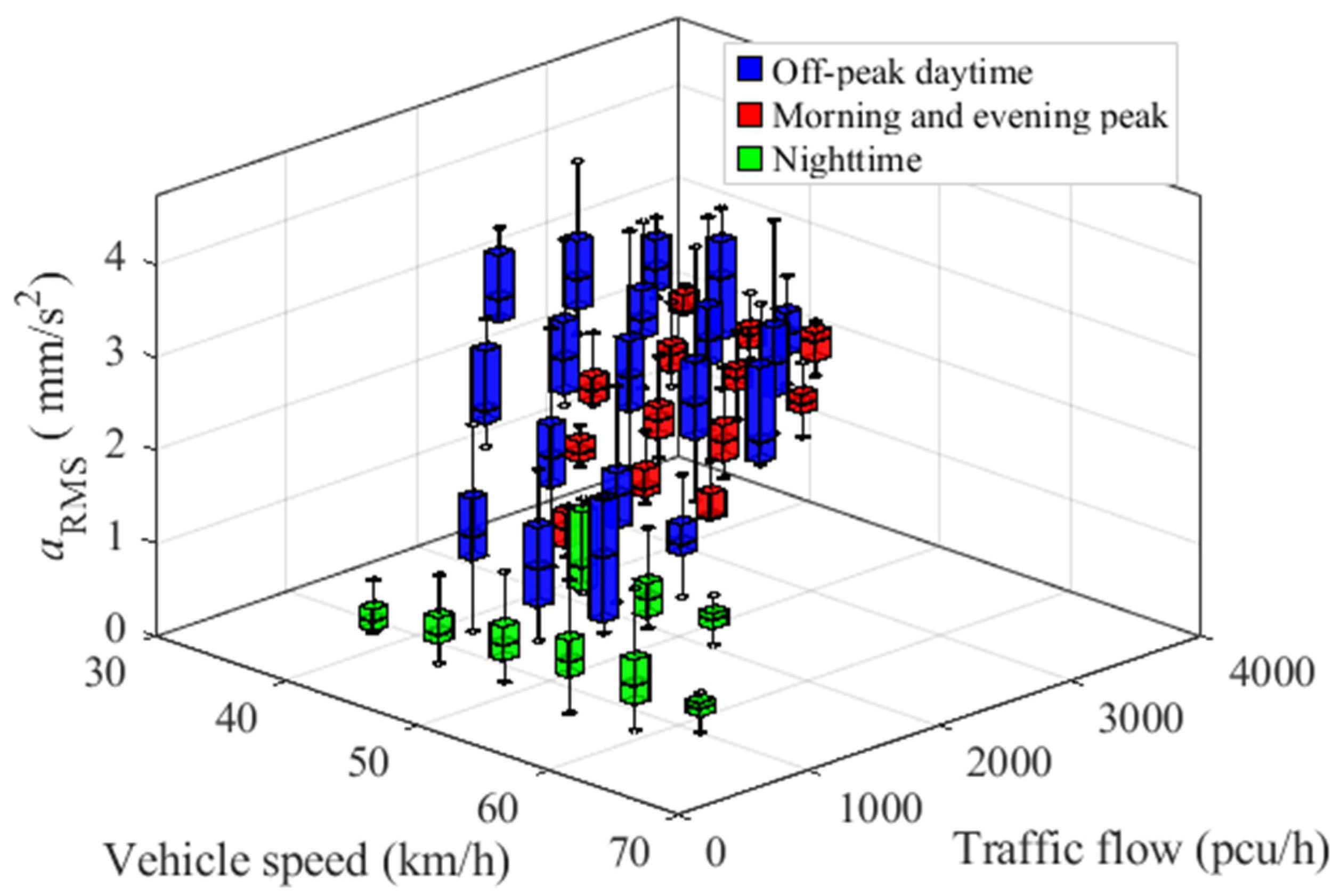
A further statistical analysis was conducted on the traffic flow and vehicle speed characteristics of the Fuzhou Pushang Bridge, and a correlation model between pier vibration responses, traffic flow, and vehicle speed was established, as shown in Figure 6. The results indicate that the pier vibration responses exhibit a complex relationship with traffic flow and vehicle speed. When traffic flow is low, although vehicle speeds are relatively high, both the vibration amplitudes and variability of the piers remain small. As traffic flow increases, vehicle speeds decrease slightly, but pier vibrations increase significantly and exhibit greater variability. With further increases in traffic flow, accompanied by a noticeable reduction in vehicle speed, pier vibrations and their variability both decrease. These patterns reflect the coupled effects of traffic density and vehicle speed on dynamic pier responses.

2.2.2. Water Level Variations

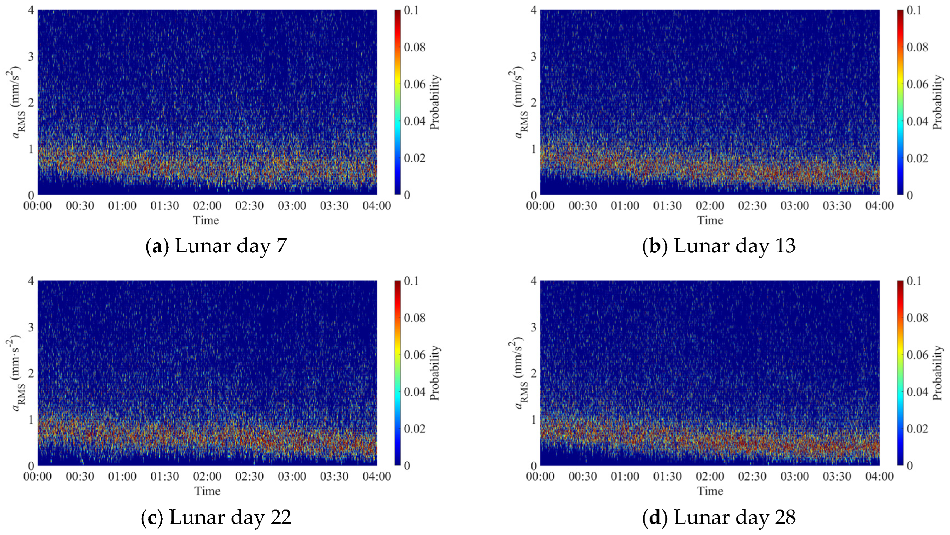
The vibration response of bridge piers is stronger during the daytime due to vehicular loads and weaker at night. Since the impact of water flow on the piers persists continuously throughout the day, the nighttime period (00:00–04:00) was selected to minimize interference from vehicular loads. According to hydrological data of the Minjiang River, the 7th and 22nd days of the lunar calendar correspond to representative phases of the tidal cycle, during which rising water levels occur and the upstream flow exhibits a backflow-dominated condition. In contrast, the 13th and 28th lunar days correspond to falling water level periods, during which downstream flow represents a dominant following-flow condition. The pier vibrations during these representative periods were therefore compared. Figure 7 shows the variation in pier vibrations during water level fluctuations. No significant correlation was observed between water level changes and pier vibrations, indicating that water level variations have a limited influence, partially masked by vehicular loads.

2.2.3. Tidal Fluctuations

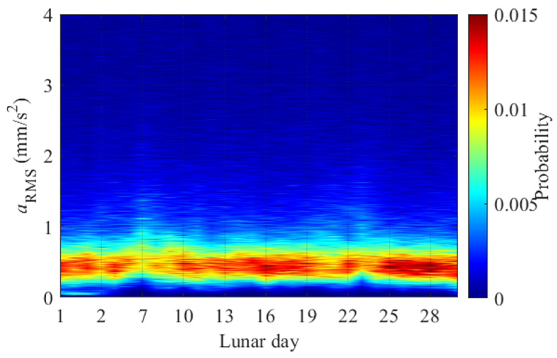
Over a complete monthly tidal cycle, the tidal range is influenced by astronomical tidal forces, exhibiting a periodic fluctuation of “spring tide—neap tide—spring tide—neap tide,” which reflects water level variations over a longer time scale. To investigate the variation characteristics of pier vibration responses within the monthly tidal cycle, the pier dynamic response indices between 03:30 and 04:30 each day were analyzed in terms of their probability distributions and arranged sequentially by date, as shown in Figure 8. It is observed that the variation amplitude of a_RMS within the monthly tidal cycle is relatively small and does not display a periodic pattern consistent with the tidal range, further indicating that water level fluctuations have a relatively limited effect on the dynamic response of the piers.

2.3. Time-Domain Features of Monitoring Data

As discussed in Section 2.2, the a_RMS exhibits a strong correlation with vehicular loads, while its sensitivity to other factors such as water level and tidal variations is comparatively limited. Due to the pronounced daily periodicity of vehicular operations, with traffic patterns being generally consistent from day to day, and the intraday variability resulting from dynamic fluctuations in traffic flow and mean vehicle speed throughout the day, the pier vibration responses correspondingly demonstrate pronounced periodic and time-dependent characteristics.

2.3.1. Daily Periodicity

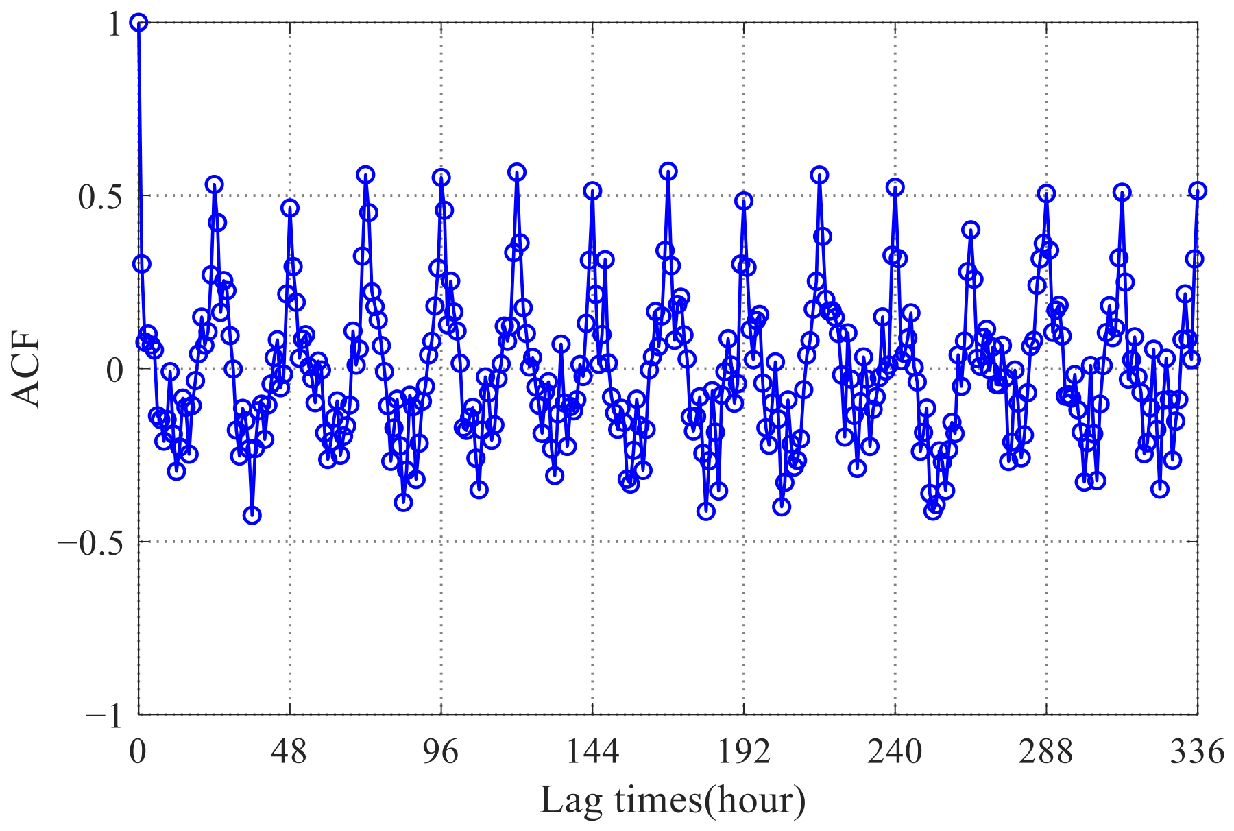
The autocorrelation coefficient (ACF) method was employed to analyze the daily periodicity of the a_RMS. This method reveals periodic patterns in the time series by calculating the correlation between the signal and its lagged values at different lags. In this study, the lag interval was set to 1 h to ensure adequate temporal resolution while covering a complete daily cycle.

Figure 9 presents the autocorrelation coefficients of the pier monitoring data. It is observed that pronounced peaks appear at lag times corresponding to integer multiples of 24 h, indicating the presence of a stable daily periodic pattern. Even at a lag of 168 h (i.e., one week), the autocorrelation coefficient remains above 0.5, demonstrating that this periodic characteristic is not only consistent on a daily basis but also maintains strong persistence and repeatability over longer durations. This property provides a solid foundation for constructing a daily scale statistical model of a_RMS.

2.3.2. Intraday Non-Stationarity

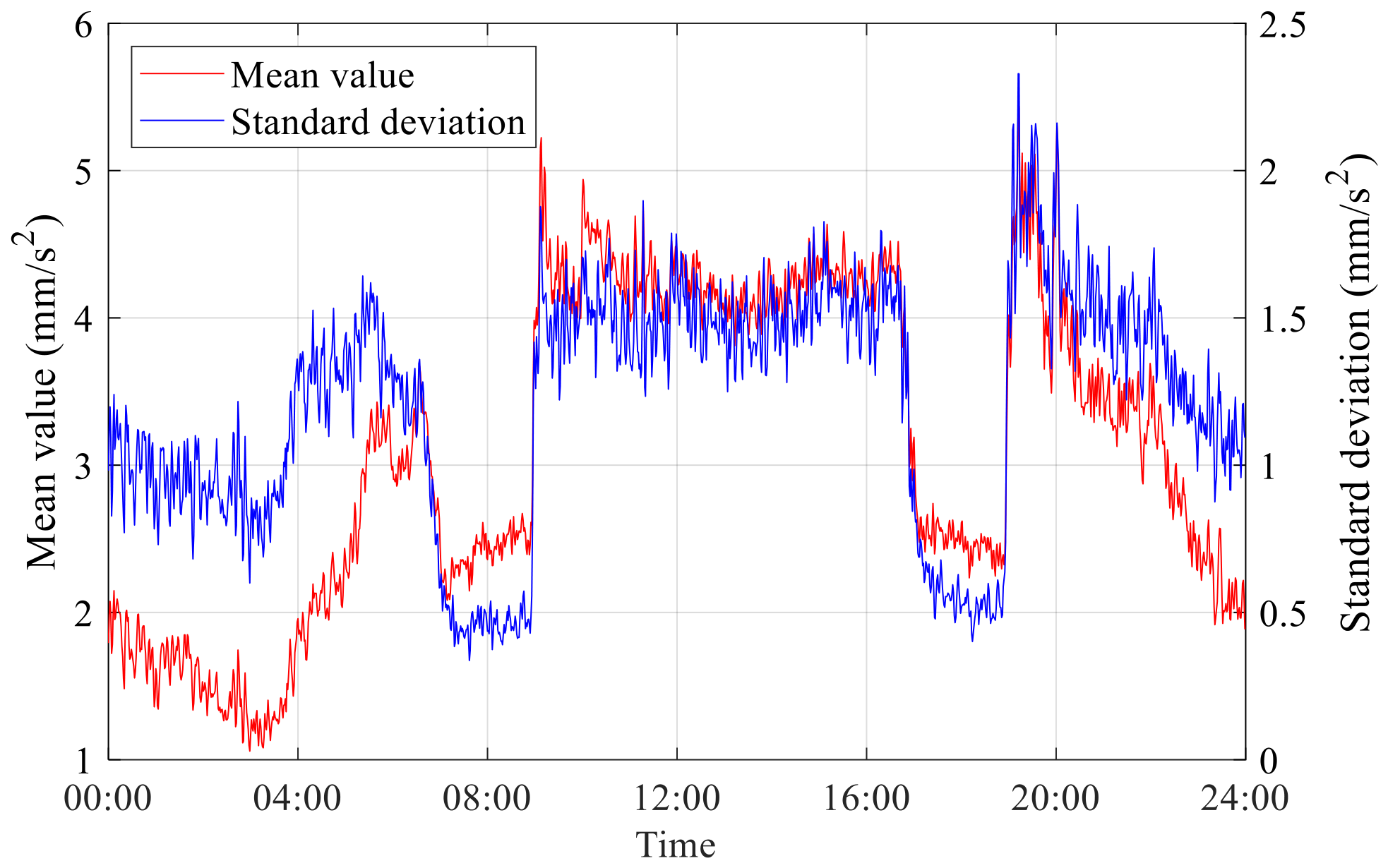
To investigate the intraday variation pattern of a_RMS in pier vibration responses, monitoring data collected over 150 days were analyzed, and the probability distributions of values at the same time across different days were statistically evaluated. Figure 10 illustrates the intraday variation in the mean and standard deviation of the a_RMS. It is observed that both the mean and standard deviation of the a_RMS vary significantly over time. Specifically, during the morning and evening peak hours (7:00–9:00 and 17:00–19:00), as well as the daytime off-peak period (9:00–17:00), the mean and standard deviation of the a_RMS remain relatively stable. In contrast, during the nighttime period (19:00–7:00 of the following day), both metrics show a decreasing trend followed by an increasing trend, attaining their minimum values around 3:00 a.m.

To further evaluate the stationarity of the a_RMS time series, the mean and standard deviation series were subjected to the Augmented Dickey–Fuller test (ADF) and the KPSS test. The null hypothesis of the ADF test assumes that the time series is non-stationary. If the test statistic is lower than the critical value, the null hypothesis is rejected, indicating that the series is stationary; otherwise, the null hypothesis cannot be rejected, suggesting that the series is non-stationary. In this study, an autoregressive model with a constant term was adopted as the regression equation, and the optimal lag order was automatically selected based on the Bayesian Information Criterion (BIC).

The null hypothesis of the KPSS test assumes that the time series is stationary. If the test statistic is smaller than the critical value, the null hypothesis cannot be rejected, indicating stationarity; otherwise, the null hypothesis is rejected, suggesting that the series is non-stationary. In this study, the lag order used for estimating the long-run variance of the residuals was automatically determined using the Newey–West method.

The stationarity test results for the mean and standard deviation of a_RMS are presented in

Table 3. Stationarity test of the mean and standard deviation of a_RMS.

Time Series	Test Method	Test Statistic	Significance Level
			1%	5%	10%
Mean value	ADF test	−2.05	−3.43	−2.86	−2.57
	KPSS test	0.23	0.22	0.15	0.12
Standard deviation	ADF test	−4.15	−3.43	−2.86	−2.57
	KPSS test	0.07	0.22	0.15	0.12

. The results show that the mean time series fails the stationarity tests, indicating significant temporal variation. In contrast, the standard deviation series passes the ADF and KPSS tests, suggesting temporal stability.

2.3.3. Non-Normality

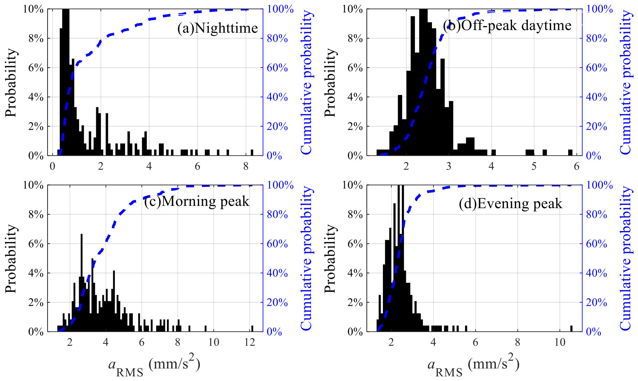
Data from typical periods within a single day, including nighttime, morning peak, daytime off-peak, and evening peak, were selected, and the probability distributions of a_RMS were analyzed, as shown in Figure 11. The Kolmogorov–Smirnov (K-S) test was employed to assess the normality of a_RMS distributions. The null hypothesis of the K-S test is that the sample follows a normal distribution. If the test statistic is smaller than the critical value, the null hypothesis cannot be rejected, indicating that the sample is normally distributed; otherwise, it is rejected, suggesting non-normality. The test results, presented in

Table 4. Normality test of the probability distribution of a_RMS.

Representative Period	K-S Statistic	Significance Level
		1%	5%	10%
Nighttime	0.2454	0.1470	0.1225	0.1103
Morning peak	0.1665
Off-peak daytime	0.1631
Evening peak	0.1975

, show that the a_RMS distributions at all typical time periods deviate from normality.

3. Anomaly Detection Method

3.1. Framework Overview

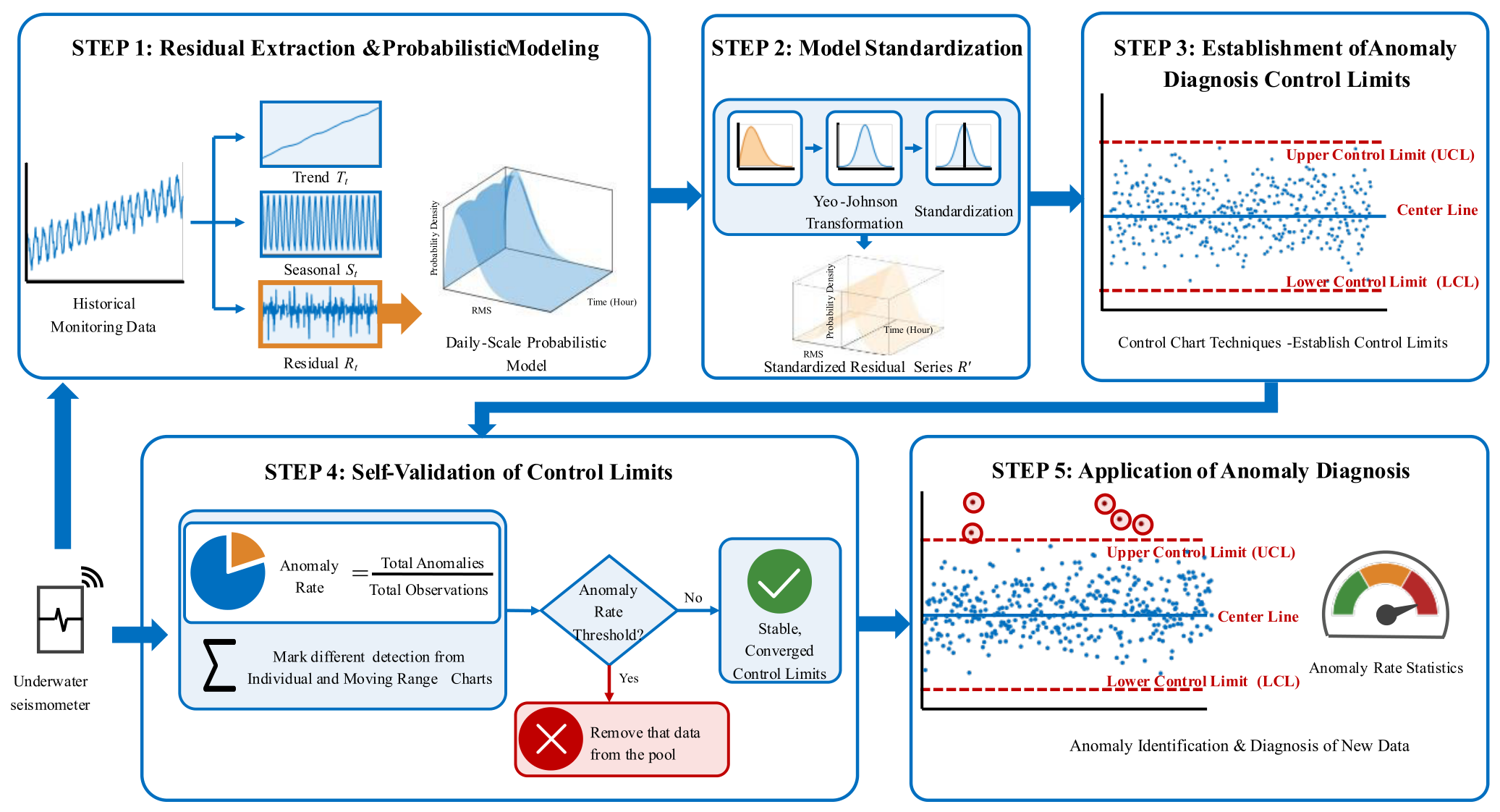
Based on the characteristics identified in Section 2, including periodicity, non-stationarity, and non-normality, a time-domain anomaly detection framework is proposed, integrating STL decomposition, Yeo–Johnson transformation, and control charts, as illustrated in Figure 12.

Step 1: Residual extraction and probabilistic modeling. A segment of historical monitoring data is selected. The a_RMS time series is decomposed via the STL method to extract its residual component R_t. At each time point within a day, the probability distribution of the residual component R_t is statistically modeled, thereby establishing a daily scale probabilistic model.

Step 2: Model standardization. The Yeo–Johnson transformation is applied to mitigate non-normality in the residual distributions. The residuals are then standardized via mean-centering and scaling by the standard deviation, yielding a standardized residual series R′, that approximately follows a standard normal distribution.

Step 3: Establishment of anomaly detection control limits. Based on the standardized residual series R′, a suitable control chart is employed, and the control limits are established at a specified significance level.

Step 4: Self-validation of control limits. The control limits are validated using historical data. The anomaly rate is defined as the proportion of detected anomalous points to the total number of observations, and a threshold is specified. Days with anomaly rates exceeding this threshold are excluded, and Steps 1–4 are iteratively repeated until the control limits converge.

Step 5: Application of anomaly detection. The finalized control limits are applied to subsequent monitoring data for anomaly detection.

In summary, the proposed framework transforms non-stationary and non-normal monitoring data into a stationary and approximately Gaussian process, enabling robust anomaly detection using statistical control theory.

3.2. STL Decomposition of Time Series

STL is a time series decomposition technique based on locally estimated scatterplot smoothing (Loess), and was first proposed by Cleveland et al. in 1990 [32,33]. It is widely used to extract and analyze the underlying components of time series. For a given time series Y_t, STL decomposes it into three additive components:

$$Y_t=T_t+S_t+R_t$$

(1)

where T_t is the trend term, representing the long-term variation in the data (such as material aging effect); S_t is the seasonal term, capturing the periodic patterns in the data; R_t is the residual term, representing random fluctuations, anomalies, and abrupt changes in the data.

Loess constitutes the core algorithm underlying STL decomposition. It enables flexible smoothing of data exhibiting nonlinear variation, without requiring a predefined functional form. The fundamental idea is to assign weights to neighboring points based on distances to a target estimation point, and fit a low-order polynomial within the local neighborhood to obtain a smoothed estimate. Let (x_i, y_i) (i = 1, 2,…, n) denote the observed data, where x_i denotes the time index and y_i the corresponding observation. The data are assumed to satisfy:

$$y_i={\displaystyle \sum _{k=0}^p{\beta }_k\left(x_i\right)\cdot x_i^k}+{\epsilon }_i$$

(2)

where ε_i is the error term, and p is the order of the polynomial, typically p = 1 for local linear regression or p = 2 for local quadratic regression. β_k(x_i) is the local regression coefficients, which are estimated by minimizing the weighted sum of squared residuals, i.e.,

$${\widehat{\beta }}_k\left(x_i\right)=\arg \underset{\beta }{\min }{{\displaystyle \sum _{j=1}^n{\omega }_{ij}\left[y_j-{\displaystyle \sum _{k=0}^p{\beta }_k\left(x_i\right){\left(x_j-x_i\right)}^k}\right]}}^2$$

(3)

where ω_ij denotes the weight of point x_j relative to the target point x_i using the tricube weight function:

$${\omega }_{ij}=\left\{\begin{array}{ll}{\left[1-{\left({\displaystyle \frac{x_j-x_i}{c}}\right)}^3\right]}^3& \left|x_j-x_i\right|<c\\ 0& otherwise\end{array}\right.$$

(4)

where c is the window width centered on x_i, determining the number of samples used in the local fitting.

Based on the local regression coefficients, the smoothed estimate ${\widehat{y}}_i$ is given by:

$${\widehat{y}}_i={\displaystyle \sum _{k=0}^p{\widehat{\beta }}_k{x}_i^k}$$

(5)

STL decomposition involves an inner loop and an outer loop. The inner loop primarily estimates the seasonal and trend term under given weights. The outer loop computes robust weights based on the residuals and feeds them back into the inner loop to reduce the influence of outliers.

Assume that the seasonal and trend terms obtained in the v-th iteration are $S_t^{\left(v\right)}$ and $T_t^{\left(v\right)}$, respectively. Then, the main steps of the (v + 1)-th inner loop are as follows:

Step 1: Remove the trend component to obtain the detrended series $Y_t-T_t^{\left(v\right)}$;

Step 2: Extract a set of cycle subseries according to the seasonal period. Loess smoothing is applied to each subseries, and the results are recombined to obtain a preliminary seasonal component, denoted as ${\tilde{S}}_t^{\left(v+1\right)}$;

Step 3: Apply a low-pass filter to ${\tilde{S}}_t^{\left(v+1\right)}$ (including two moving averages with a window length equal to the seasonal period, followed by one moving average with a window length of 3, and a Loess smoothing) to obtain the low-frequency component, denoted as $L_t^{\left(v+1\right)}$;

Step 4: Remove the low-frequency component $L_t^{\left(v+1\right)}$ from ${\tilde{S}}_t^{\left(v+1\right)}$ to obtain the seasonal component $S_t^{\left(v+1\right)}$;

Step 5: Remove the seasonal component $S_t^{\left(v+1\right)}$ to obtain the deseasonalized component $Y_t-S_t^{\left(v+1\right)}$;

Step 6: Apply Loess smoothing to the deseasonalized component to update the trend component $T_t^{\left(v+1\right)}$.

After completing one iteration of the inner loop, the residual component can be calculated as $R_t^{\left(v+1\right)}=Y_t-S_t^{\left(v+1\right)}-T_t^{\left(v+1\right)}$.

In the outer loop, the robustness weights ρ_t for Y_t need to be determined to reduce the influence of outliers:

$${\rho }_t={\displaystyle \frac{B\left(\left|R_t\right|\right)}{h}}$$

(6)

$$h=6\times median\left(\left|R_t\right|\right)$$

(7)

where $B\left(\left|R_t\right|\right)$ is defined by the bisquare function, expressed as:

$$B\left(\left|R_t\right|\right)=\left\{\begin{array}{cc}{\left(1-{\left|R_t\right|}^2\right)}^2& 0\le \left|R_t\right|<1\\ 0& \left|R_t\right|\ge 1\end{array}\right.$$

(8)

Applying ρ_t in Step 2 and Step 6 can effectively reduce the influence of outliers on the regression.

3.3. Yeo–Johnson Transformation

The Yeo–Johnson transformation, proposed by I. K. Yeo and R. A. Johnson in 2000 [34], is an extension of the Box–Cox transformation that can handle both positive and negative values. Its fundamental objective is to adjust the distributional shape of the data through a parametric power transformation, thereby approximating normality and improving data stability. For a given observation Y, the transformation is defined as:

$$\mathrm{\Psi }=\left\{\begin{array}{ll}{\displaystyle \frac{{\left(Y+1\right)}^r-1}{\lambda }}& ifY\ge 0,r\ne 0\\ \log \left(Y+1\right)& ifY\ge 0,r=0\\ {\displaystyle \frac{1-{\left(-Y+1\right)}^{2-r}}{2-r}}& ifY<0,r\ne 2\\ -\log \left(-Y+1\right)& ifY<0,r=2\end{array}\right.$$

(9)

where r is the transformation parameter, and its optimal value is determined by maximum likelihood estimation (MLE).

3.4. Control Chart-Based Anomaly Detection

Control chart methods are time-series quality monitoring approaches based on statistical process control. They involve continuously plotting process statistics (such as the mean, range, or individual values) to determine whether the process is under statistical control. A control chart typically consists of a center line (CL), an upper control limit (UCL), and a lower control limit (LCL). Control limits are typically set at ±3σ (corresponding to 99.73%) to identify abnormal variations. If observed values fall within the control limits and exhibit a random pattern, the process is considered to be in control. Conversely, if data points exceed the control limits or display non-random patterns, it indicates that the process may be affected by abnormal disturbances. Because they can simultaneously capture random fluctuations and structural changes, control charts are widely used in fields such as industry, healthcare, and structural health monitoring for real-time anomaly detection and process stability assessment [35].

The Individuals–Moving Range (I–MR) control chart is a type of control chart suitable for situations where only a single observation can be obtained at a time and rational subgrouping is not feasible, such as online monitoring, high-value low-frequency measurements, or destructive testing. Let the sample z_t come from a normally distributed population Z~N(μ, σ). When the sample size is 1, the process standard deviation is typically estimated using the moving range of consecutive observations. Based on this, the process mean serves as the center line, and the upper and lower control limits are constructed according to the ±3σ principle to determine whether the process is under statistical control.

The control limits of the individuals control chart are given by:

$$\left\{\begin{array}{c}CL=\overline{Z}\\ U_{\mathrm{CL}}=\overline{Z}+2.660\overline{MR}\\ L_{\mathrm{CL}}=\overline{Z}-2.660\overline{MR}\end{array}\right.$$

(10)

where $\overline{Z}$ is the sample mean, and $\overline{MR}$ is the moving range, defined as:

$$\overline{MR}={\displaystyle \frac{{\displaystyle \sum _{t=2}^N{R}_t}}{N-1}}={\displaystyle \frac{{\displaystyle \sum _{t=2}^N\left|z_t-z_{t-1}\right|}}{N-1}}$$

(11)

The control limits of the moving range control chart are given by:

$$\left\{\begin{array}{c}CL=\overline{MR}\\ U_{\mathrm{CL}}=3.267\overline{MR}\\ L_{\mathrm{CL}}=0\end{array}\right.$$

(12)

4. Field Validation

To evaluate the effectiveness and robustness of the proposed anomaly detection framework, long-term monitoring data from the Fuzhou Pushang Bridge were used for validation. The control limits were established using historical data, and the performance of the method was assessed through both self-validation and application to subsequent monitoring periods.

4.1. Model Performance Evaluation

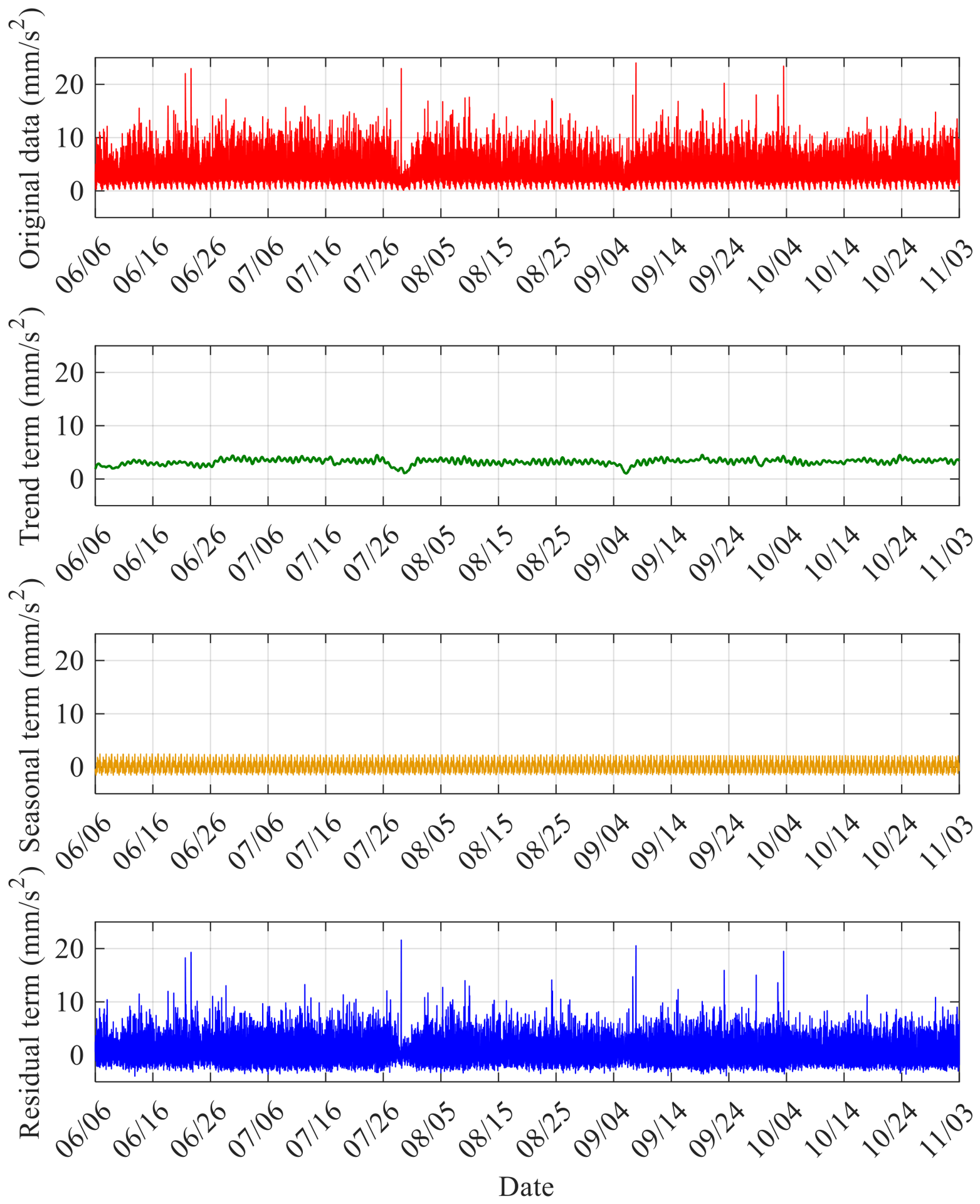
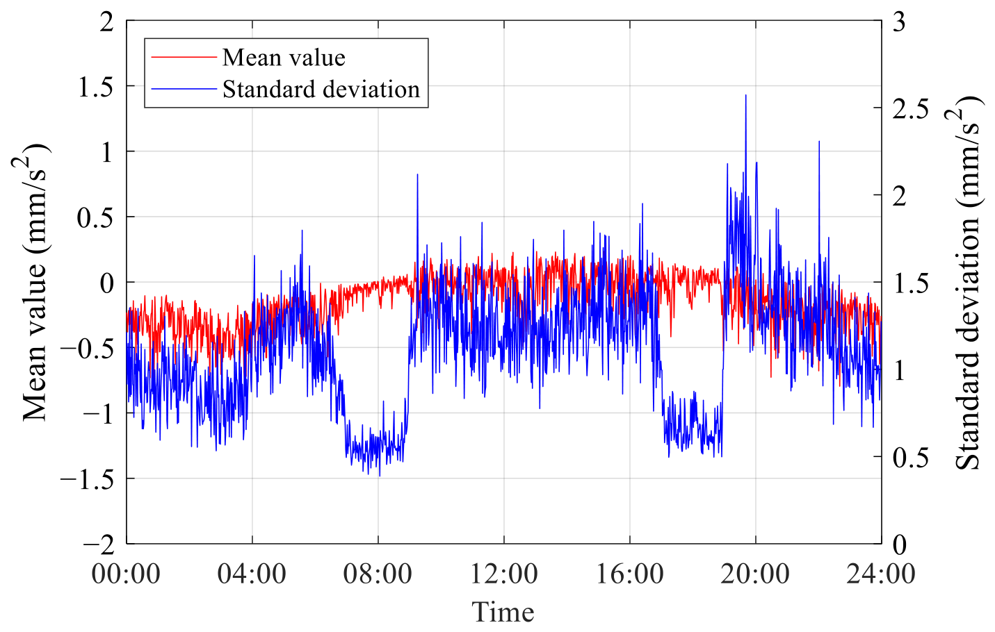
The control limits for anomaly detection were established using 150 days of monitoring data collected from 6 June 2023 to 3 November 2023. First, the STL decomposition method was applied, with the trend and seasonal smoothing windows set to 1 day and 60 min, respectively, and the number of inner iterations set to 1, considering that the monitoring data exhibit pronounced daily periodicity and intra-day variability; accordingly, these parameter choices enable effective separation of trend and seasonal components while reducing computational cost and maintaining sufficient decomposition accuracy. The decomposition results are shown in Figure 13. The residual term was then extracted to characterize stochastic fluctuations and potential anomalies. The intraday variation patterns of its mean and standard deviation were then analyzed (as shown in Figure 14). Stationarity was further evaluated using the ADF test and KPSS test (as listed in

Table 5. Stationarity test of the probability distribution of residual term.

Time Series	Test Method	Test Statistic	Significance Level
			1%	5%	10%
Mean value	ADF test	−4.14	−3.43	−2.86	−2.57
	KPSS test	0.19	0.22	0.15	0.12
Standard deviation	ADF test	−8.41	−3.43	−2.86	−2.57
	KPSS test	0.05	0.22	0.15	0.12

), respectively. The results confirm that both the mean and variance of the residual term remain stable within a daily timescale, satisfying the assumption of stationarity required for subsequent analysis.

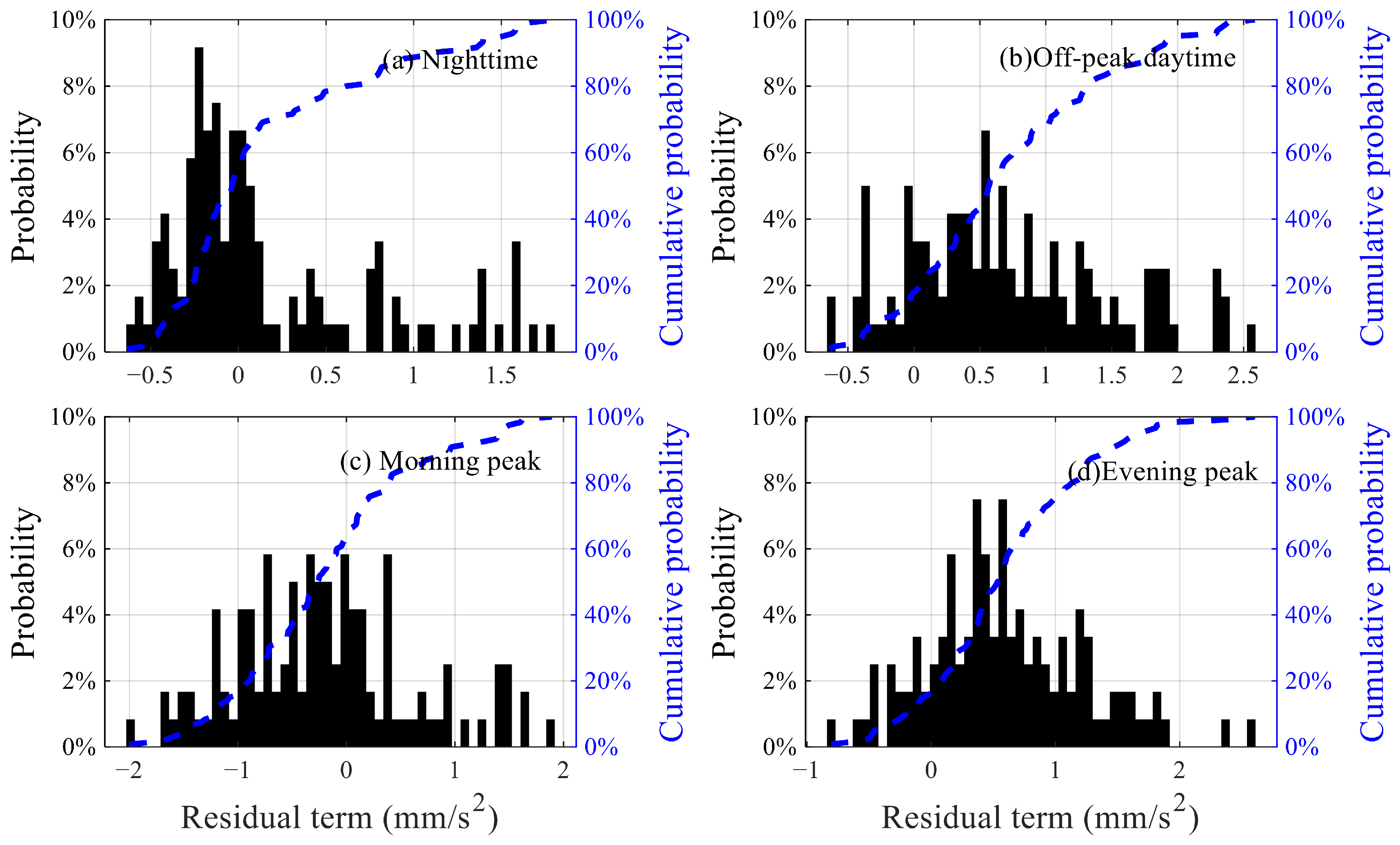
The residual term underwent the Yeo–Johnson transformation, and was then standardized by mean-centering and scaling by the standard deviation. The probability distributions for representative time periods were subsequently analyzed (as shown in Figure 15), and normality was tested (as presented in

Table 6. Normality test of the probability distribution of residual term.

Representative Period	K-S Statistic	Significance Level
		1%	5%	10%
Nighttime	0.1004	0.1470	0.1225	0.1103
Morning peak	0.0796
Off-peak daytime	0.0715
Evening peak	0.0955

). This confirms that the proposed preprocessing steps effectively address the non-normality of the original data.

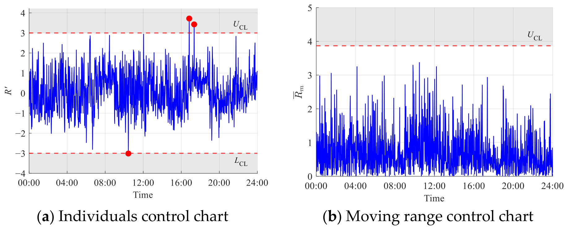
Anomaly detection was performed using the I-MR control chart. According to Equations (10) and (12), the control limits for the individuals and moving range charts were established. The constructed chart was validated using historical data, as shown in Figure 16. The results show that the anomaly rates on 16 July and 28 July exceed 1%; therefore, the data from these two days were removed. After removal, the intrinsic anomaly rate of the model is 0.14%, which is in good agreement with the theoretical value of 0.27% under the ±3σ control limit, confirming the suitability of the proposed model for anomaly detection.

4.2. Anomaly Detection

4.2.1. Normal Conditions

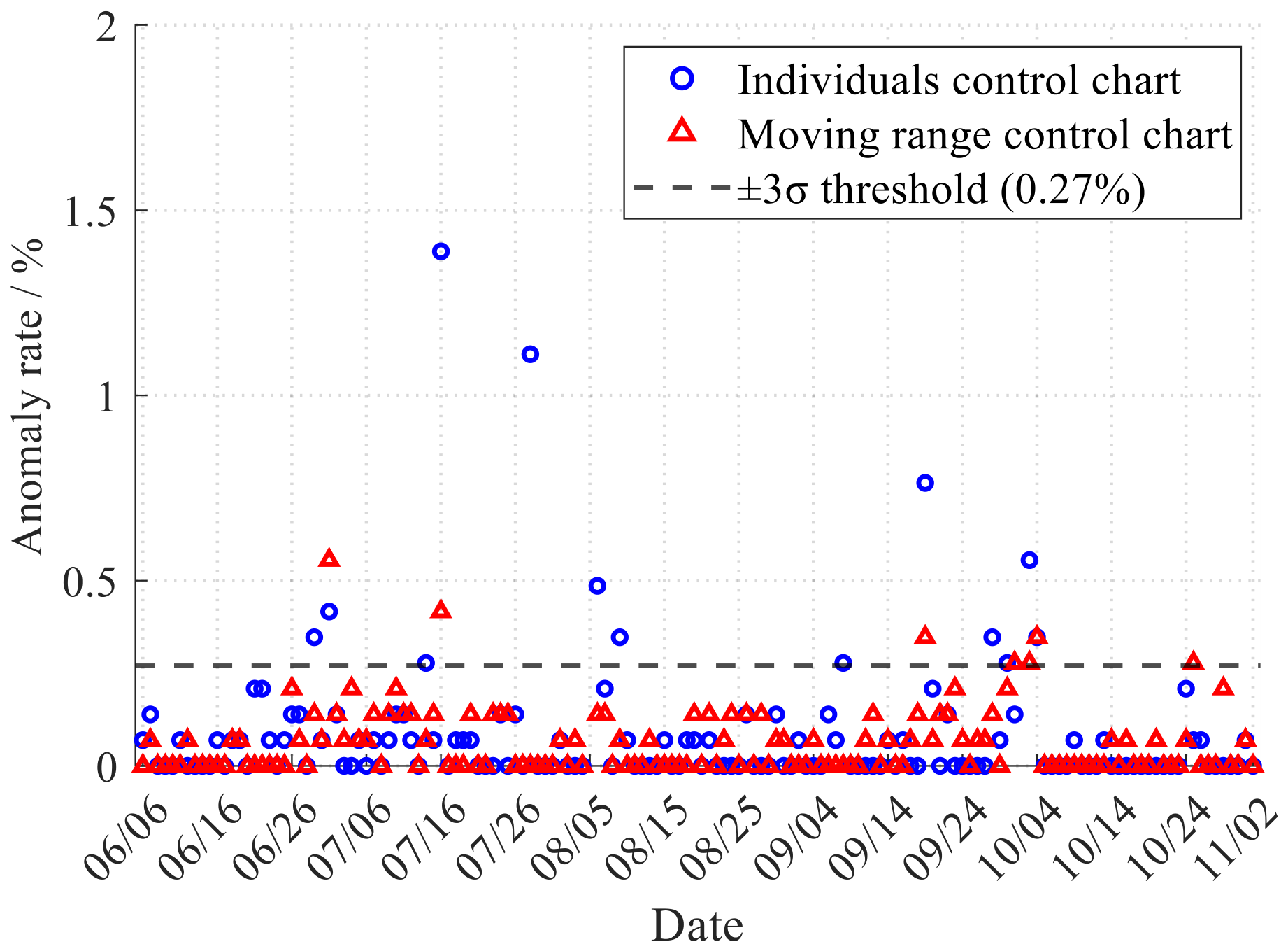
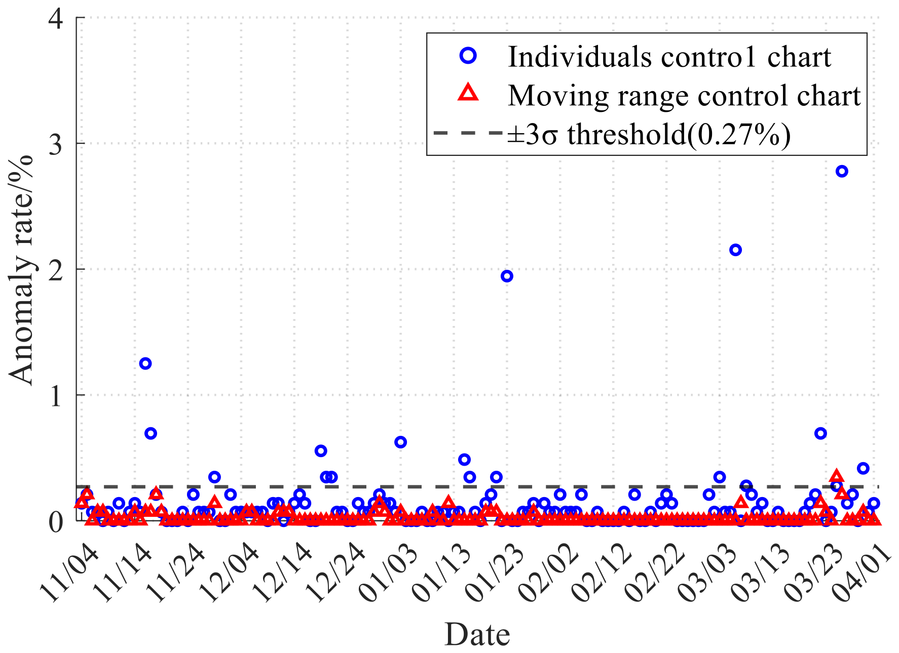
The established control limit was applied to detect anomalies in the following 150 days of monitoring data, covering the period from 4 November 2023 to 1 April 2024. Figure 17 presents the anomaly rate over this period. The calculated anomaly rate is approximately 0.18%, indicating that the monitoring data acquired by the underwater seismometer exhibit no significant abnormalities.

Further analysis was performed on the data with anomaly rates exceeding 1.0%. Figure 18 shows typical abnormal data observed under normal conditions. Field inspections indicate that these anomalies are primarily related to the operational state of the underwater seismometer under tidal fluctuations in the lower reaches of the Minjiang River, where the water level varies significantly and the sensor is not always fully submerged. Two mechanisms are identified. First, when the instrument is partially exposed above the water surface, it is directly subjected to river flow action, resulting in an increase in the recorded vibration amplitude. However, such hydrodynamic loading does not necessarily lead to exceedance of the anomaly threshold, depending on the instantaneous flow intensity and local hydraulic conditions. Second, transient hydrodynamic disturbances, such as impulsive impacts from floating debris or localized turbulent fluctuations, may induce short-duration response peaks that exceed the predefined threshold, thereby appearing as isolated anomalous data points.

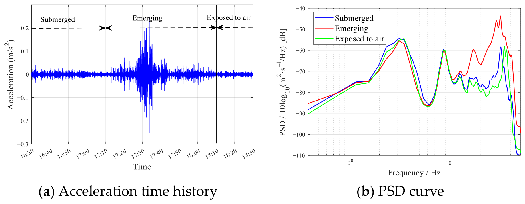
The underwater seismometer data under different operating conditions were compared (as shown in Figure 19a). It is observed that during the transient stages of entering or emerging from the water surface, the measured vibration amplitude is significantly higher than during periods of stable submersion or full exposure. Further analysis of the corresponding power spectral density (PSD) curves (as shown in Figure 19b) indicates that, in these transient stages, the frequency energy around 32 Hz is markedly amplified. Structural dynamic analysis suggests that this frequency band does not correspond to the natural frequencies of the structure and is likely induced by non-structural disturbances from fluid impacts at the air–water interface on the instrument. Therefore, for subsequent structural dynamic identification and safety assessments, data from these periods should be identified and excluded to avoid interference and to ensure the accuracy and reliability of monitoring results.

4.2.2. Extreme Events

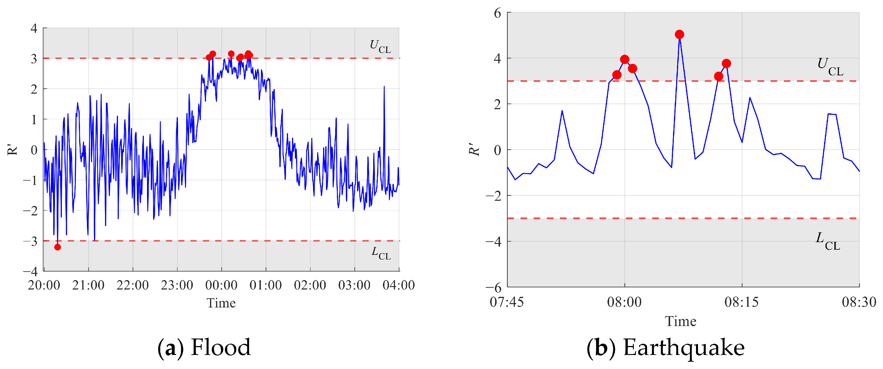
To verify the capability of the proposed method in identifying extreme events such as floods and earthquakes, extreme events occurring during the monitoring period were analyzed. The application results indicate that all the aforementioned conditions were successfully identified. Figure 20a shows the anomaly detection results under flood conditions. It is observed that the monitoring data during the nighttime period exhibit concentrated anomalies, with the control chart statistics initially increasing and subsequently decreasing between 23:00 and 02:00 the following day, and the anomaly rate reaching 4.44%, which is significantly higher than that under normal operating conditions. Figure 20b shows the anomaly detection results under a typical earthquake condition. It is seen that the maximum value of the control chart statistics reached 5.03 during the earthquake, clearly exceeding the control limit of 3.0. Overall, these results demonstrate that the proposed method can effectively capture structural responses during transient stages of extreme events, providing support for structural safety assessment and risk warning under special operating conditions.

4.3. Compared with the Percentile-Based Method

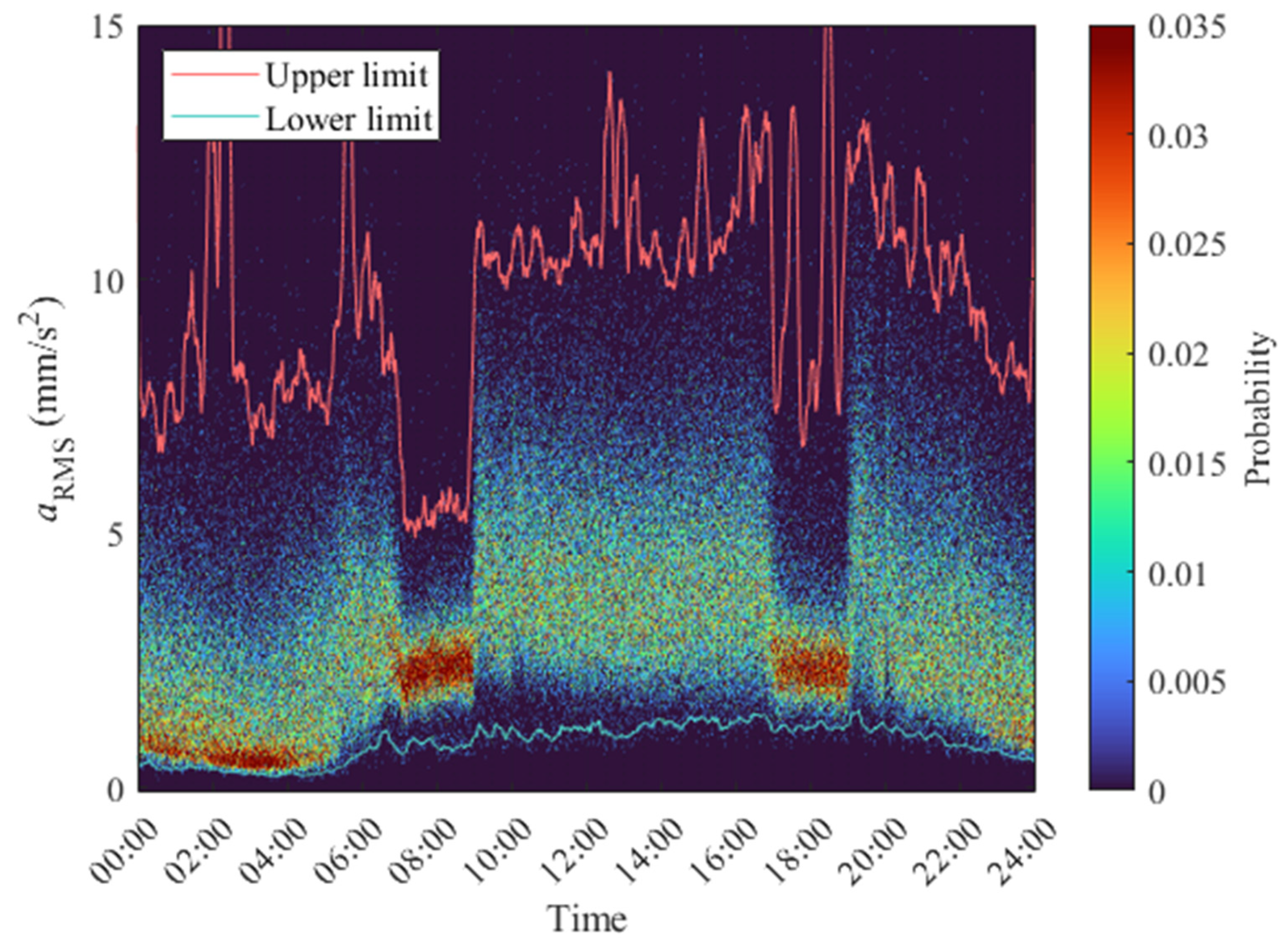
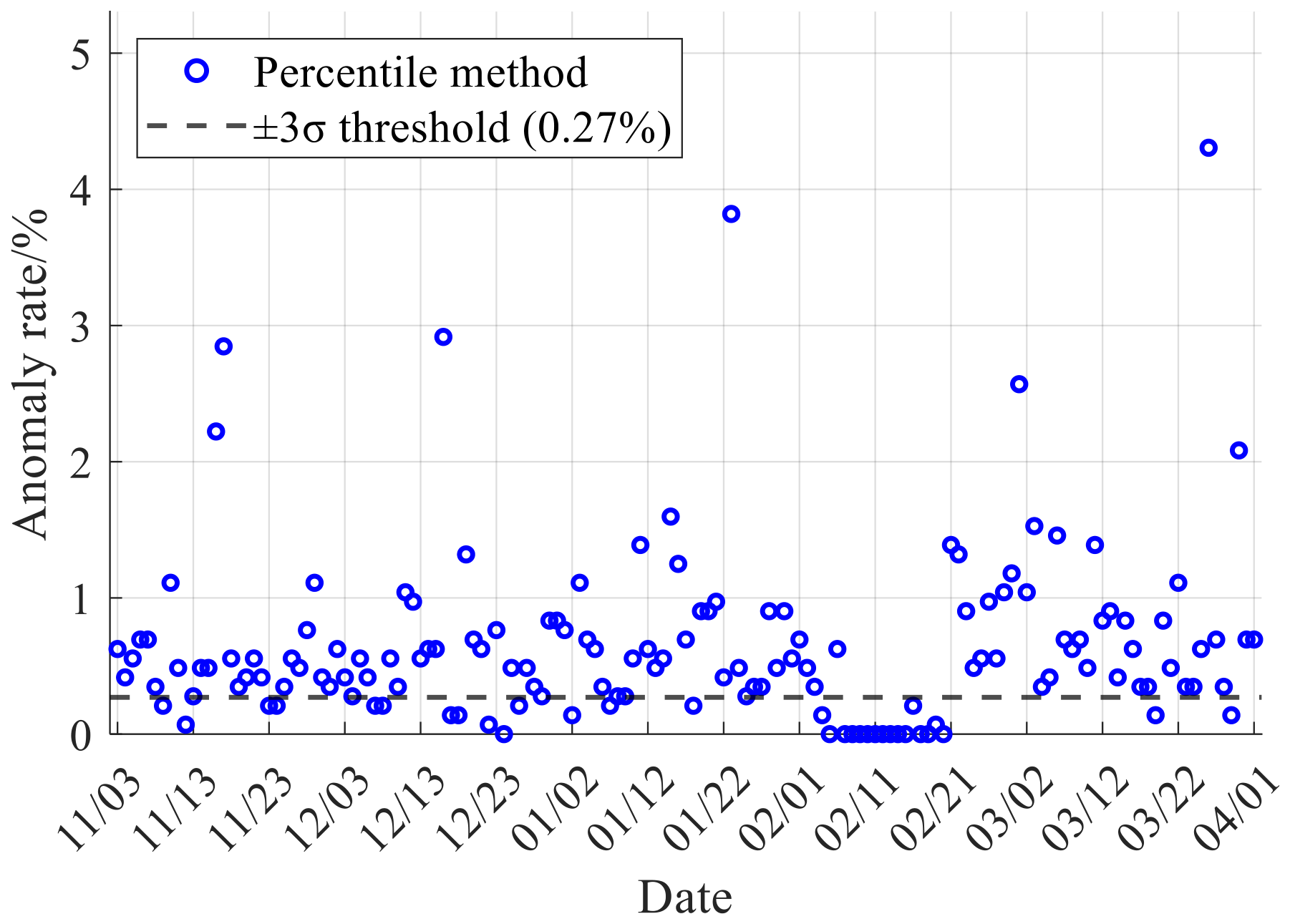
The proposed method was compared with the percentile-based method. The percentile-based method identifies anomalies based on the tails of the data distribution: for a given discrete sequence of observations, the data are first sorted in ascending order, and upper and lower thresholds were determined according to preset quantiles. Data exceeding these thresholds were considered abnormal. To match the theoretical probability corresponding to the control limits of the proposed method, the upper and lower thresholds of the percentile-based method were set to 99.865% and 0.135%, respectively, resulting in a constant anomaly rate of 0.27% during self-validation.

Using the same 150-day monitoring dataset, the probability distribution of a_RMS at the same time each day was calculated to construct a daily scale statistical model. The corresponding upper and lower thresholds were then determined, as shown in Figure 21, and anomaly detection was subsequently performed, as shown in Figure 22. The anomaly rate calculated by the percentile-based method was 0.65%, indicating a higher false alarm rate. These results demonstrate that the proposed method has better generalization capability, allowing control limits to be established using short-term data and applied to long-term monitoring.

5. Conclusions

This study investigates vibration monitoring data collected from underwater seismometers installed on a cross-river bridge and proposes a time-domain anomaly detection framework. The main conclusions are summarized as follows:

(1)

The vibration response of bridge piers is predominantly governed by vehicular loads, while the effects of water level and tidal fluctuations are comparatively minor. The monitoring data exhibit pronounced daily periodicity, intraday non-stationarity, and non-normality.

(2)

The proposed framework, integrating STL decomposition, Yeo–Johnson transformation, and control charts, effectively transforms the original data into a stationary and approximately normally distributed process. The self-validation anomaly rate (0.14%) is consistent with the theoretical expectation, demonstrating the statistical reliability of the method.

(3)

Application to long-term monitoring data yields an anomaly rate of 0.18%, confirming the stability and robustness of the method. Detected anomalies are mainly associated with hydrodynamic impacts during transitions between submerged and exposed conditions.

(4)

Under extreme events, such as floods and earthquakes, the proposed method successfully captures significant abnormal responses, demonstrating strong sensitivity to both gradual and abrupt disturbances.

(5)

Compared with the percentile-based method, the proposed approach exhibits a lower false alarm rate and better generalization capability, making it more suitable for long-term structural health monitoring applications.

In summary, the proposed method provides a reliable and practical solution for anomaly detection in underwater vibration monitoring data. It can be extended to other infrastructure systems operating under complex environmental conditions.

Despite its effectiveness, several aspects warrant further investigation. Future work will focus on conducting a systematic sensitivity analysis of key parameters, including the a_RMS sliding window length, the size of historical training data, and the selection of control chart types, in order to quantitatively assess their influence on detection performance. In addition, the proposed method will be validated across multiple engineering projects with varying structural types and environmental conditions to further evaluate its robustness and generalizability.

Furthermore, the proposed framework is fundamentally data-driven and does not rely on bridge-type-specific mechanical assumptions, suggesting its potential applicability to various bridge types (e.g., beam, arch, and cable-supported bridges) given sufficient monitoring data. However, environmental factors such as temperature, humidity, wind, and traffic loading may affect the statistical characteristics of the data. In more complex or variable environments, additional preprocessing or adaptive parameter tuning may be required to ensure robustness. Future work will further validate the method across diverse bridge types and environmental conditions.

References

1. Zhang, B.; Ren, Y.; He, S.; Gao, Z.; Li, B.; Song, J. A review of methods and applications in structural health monitoring (SHM) for bridges. Measurement 2025, 245, 116575. [Google Scholar] [CrossRef]
2. Saidin, S.S.; Jamadin, A.; Kudus, S.A.; Amin, N.M.; Anuar, M.A. An Overview: The application of vibration-based techniques in bridge structural health monitoring. Int. J. Concr. Struct. Mater. 2022, 16, 69. [Google Scholar] [CrossRef]
3. Nord, T.S.; Petersen, Y.W.; Hendrikse, H. Stochastic subspace identification of modal parameters during ice-structure interaction. Philos. Trans. R. Soc. A 2019, 377, 20190030. [Google Scholar] [CrossRef] [PubMed]
4. Sibille, L.; Nord, T.S.; Frøseth, G.T.; Fenerci, A.; Siedziako, B. Characterization and analysis of ferry impacts on the Magerholm ferry quay. Measurement 2026, 257, 118551. [Google Scholar] [CrossRef]
5. Zhang, L.; Lu, T.; Wang, F.; Xia, Y. Over 25-year monitoring of the Tsing Ma suspension bridge in Hong Kong. J. Civ. Struct. Health Monit. 2025, 15, 263–283. [Google Scholar] [CrossRef]
6. Liu, J.; Liang, P.; He, M.; Shi, Z.; Zhou, Z.; Liang, Z. Innovations of structural health monitoring system: Application in Hong Kong-Zhuhai-Macao bridge. Struct. Infrastruct. Eng. 2025, 1–16. [Google Scholar] [CrossRef]
7. Fujino, Y.; Siringoringo, D.M.; Ikeda, Y.; Nagayama, T.; Mizutani, T. Research and implementations of structural monitoring for bridges and buildings in Japan. Engineering 2019, 5, 1093–1119. [Google Scholar] [CrossRef]
8. Li, Z.K.; Lin, W.W.; Kim, C.W.; Limongelli, M.P. A comprehensive review of indirect bridge health monitoring. Mech. Syst. Signal Process. 2026, 247, 113918. [Google Scholar] [CrossRef]
9. Sun, Z.; Mahmoodian, M.; Sidiq, A.; Jayasinghe, S.; Shahrivar, F.; Setunge, S. Optimal sensor placement for structural health monitoring: A comprehensive review. J. Sens. Actuator Netw. 2025, 14, 22. [Google Scholar] [CrossRef]
10. Rizzo, P.; Enshaeian, A. Challenges in bridge health monitoring: A review. Sensors 2021, 21, 4336. [Google Scholar] [CrossRef]
11. Yang, Y.; Chen, T.; Lin, W.; Jing, M.; Xu, W. Research progress on calibration of bridge structural health monitoring sensing system. Adv. Bridge Eng. 2024, 5, 32. [Google Scholar] [CrossRef]
12. Li, X.; Meng, Q.; Wei, M.; Sun, H.; Zhang, T.; Su, R. Identification of underwater structural bridge damage and BIM-based bridge damage management. Appl. Sci. 2023, 13, 1348. [Google Scholar] [CrossRef]
13. Sasidharan, M.; Parlikad, A.K.; Schooling, J.; Hadjidemetriou, G.M.; Hamer, M.; Kirwan, A.; Roffe, S. A bridge scour risk management approach to deal with uncertain climate future. Transp. Res. Part D Transp. Environ. 2023, 114, 103567. [Google Scholar] [CrossRef]
14. FHWA. National Bridge Inventory, Deficient Bridges by Highway System in 2017. Federal Highway Administration. 2018. Available online: https://www.fhwa.dot.gov/bridge/nbi/no10/defbr17.cfm (accessed on 8 September 2019).
15. Liu, D.; Yang, T.; Wang, Y.; Wu, Y.; Huang, X. Pankun: A new generation of broadband ocean bottom seismograph. Sensors 2023, 23, 4995. [Google Scholar] [CrossRef]
16. Wang, Y.; Yang, T.; Wu, Y.; Liu, D.; Huang, X.; Wang, J.; Zhong, W.; Shou, H.; Zhou, Y.; Chen, Y. A new broadband ocean bottom seismograph and characteristics of the seismic ambient noise on the South China Sea seafloor based on its recordings. Geophys. J. Int. 2022, 230, 684–695. [Google Scholar] [CrossRef]
17. Shiobara, H.; Kanazawa, T.; Isse, T. New step for broadband seismic observation on the seafloor: BBOBS-NX. IEEE J. Ocean. Eng. 2013, 38, 396–405. [Google Scholar] [CrossRef]
18. Satyavani, N.; Sain, K.; Gupta, H.K. Ocean bottom seismometer data modeling to infer gas hydrate saturation in Krish-na-Godavari (KG) basin. J. Nat. Gas Sci. Eng. 2016, 33, 908–917. [Google Scholar] [CrossRef]
19. Shinohara, M.; Ichihara, M.; Sakai, S.; Yamada, T.; Takeo, M.; Sugioka, H.; Nagaoka, Y.; Takagi, A.; Morishita, T.; Ono, T.; et al. Continuous seismic monitoring of Nishinoshima volcano, Izu-Ogasawara, by using long-term ocean bottom seismometers. Earth Planets Space 2017, 69, 159. [Google Scholar] [CrossRef]
20. Deng, Y.; Zhao, Y.; Ju, H.; Yi, T.-H.; Li, A. Anomaly detection for structural health monitoring: State-of-the-art review. Dev. Built Environ. 2024, 17, 100337. [Google Scholar] [CrossRef]
21. Jian, X.; Zhong, H.; Xia, Y.; Sun, L. Faulty data detection and classification for bridge structural health monitoring via statistical and deep-learning approach. Struct. Control Health Monit. 2021, 28, e2824. [Google Scholar] [CrossRef]
22. Qu, B.; Liao, P.; Huang, Y. Outlier Detection and Forecasting for Bridge Health Monitoring Based on Time Series Intervention Analysis. Struct. Durab. Health Monit. 2022, 16, 323–341. [Google Scholar] [CrossRef]
23. Deng, Y.; Ju, H.; Zhong, G.; Li, A.; Ding, Y. A general data quality evaluation framework for dynamic response monitoring of long-span bridges. Mech. Syst. Signal Process. 2023, 200, 110514. [Google Scholar] [CrossRef]
24. Huang, M.S.; Zhao, W.; Gu, J.F.; Lei, Y. Damage identification of a steel frame based on integration of time series and neural net-work under varying temperatures. Adv. Civ. Eng. 2020, 2020, 4284381. [Google Scholar] [CrossRef]
25. Huang, M.S.; Zhang, J.W.; Hu, J.L.; Ye, Z. Nonlinear modeling of temperature-induced bearing displacement of long-span sin-gle-pier rigid frame bridge based on DCNN-LSTM. Case Stud. Therm. Eng. 2024, 53, 103897. [Google Scholar] [CrossRef]
26. Huang, M.S.; Wan, N.; Zhu, H.P. Reconstruction of structural acceleration response based on CNN-BiGRU with squeeze-and-excitation under environmental temperature effects. J. Civ. Struct. Health Monit. 2025, 15, 985–1003. [Google Scholar] [CrossRef]
27. Yang, N.; Qian, X. Prediction of monitoring data and state assessment of heritage stone-timber structures based on spa-tio-temporal graph neural networks. Eng. Struct. 2025, 338, 120619. [Google Scholar] [CrossRef]
28. Deng, Y.; Ju, H.; Zhai, W.; Li, A.; Ding, Y. Correlation model of deflection, vehicle load, and temperature for in-service bridge using deep learning and structural health monitoring. Struct. Control Health Monit. 2022, 29, e3113. [Google Scholar] [CrossRef]
29. Miao, C.Q.; Wang, M.; Tian, H.J.; Feng, Z.-X.; Chen, C. Damage alarming of long-span suspension bridge based on GPS-RTK monitoring. J. Cent. South Univ. 2015, 22, 2800–2808. [Google Scholar] [CrossRef]
30. Chen, X.; Yin, J.; Pennington, C.; Wu, Q.; Zhan, Z. Effect of time window and spectral measurement options on empirical Green’s function analysis using DAS array and seismic stations. Bull. Seism. Soc. Am. 2025, 115, 1255–1266. [Google Scholar] [CrossRef]
31. Aquib, T.A.; Sivasubramonian, J.; Mai, P.M. Analysis of ground motion intensity measures and selection techniques for estimat-ing building response. Appl. Sci. 2022, 12, 12089. [Google Scholar] [CrossRef]
32. Cleveland, R.B.; Cleveland, W.S.; McRae, J.E.; Terpenning, I. STL: A seasonal-trend decomposition. J. Off. Stat. 1990, 6, 3–73. [Google Scholar]
33. Dragomiretskiy, K.; Zosso, D. Variational mode decomposition. IEEE Trans. Signal Process. 2013, 62, 531–544. [Google Scholar] [CrossRef]
34. Yeo, I.; Johnson, R.A. A new family of power transformations to improve normality or symmetry. Biometrika 2000, 87, 954–959. [Google Scholar] [CrossRef]
35. Sałaciński, T.; Chrzanowski, J.; Chmielewski, T. Statistical Process Control Using Control Charts with Variable Parameters. Processes 2023, 11, 2744. [Google Scholar] [CrossRef]
Figure 1. Overview of Fuzhou Pushang Bridge.
Buildings 16 02107 g001
Figure 2. Vibration monitoring system of the Fuzhou Pushang Bridge.
Buildings 16 02107 g002
Figure 3. Typical acceleration time history.
Buildings 16 02107 g003
Figure 4. Daily intraday variation characteristics of aRMS.
Buildings 16 02107 g004
Figure 5. Statistical characteristics of aRMS in different time periods.
Buildings 16 02107 g005
Figure 6. Relationship between acceleration aRMS, traffic flow, and vehicle speed.
Buildings 16 02107 g006
Figure 7. Variation in aRMS during rising and falling tides.
Buildings 16 02107 g007
Figure 8. Variation in aRMS during a tidal cycle.
Buildings 16 02107 g008
Figure 9. Autocorrelation coefficients of aRMS.
Buildings 16 02107 g009
Figure 10. Intraday variation in aRMS mean and standard deviation.
Buildings 16 02107 g010
Figure 11. Histograms of the probability distributions of aRMS.
Buildings 16 02107 g011
Figure 12. Flowchart of the proposed anomaly detection method.
Buildings 16 02107 g012
Figure 13. STL decomposition results.
Buildings 16 02107 g013
Figure 14. Intraday variations in mean and standard deviation of residual term.
Buildings 16 02107 g014
Figure 15. Histogram of the probability distribution of residual term.
Buildings 16 02107 g015
Figure 16. Self-validation of control chart.
Buildings 16 02107 g016
Figure 17. Anomaly rate of monitoring data.
Buildings 16 02107 g017
Figure 18. Abnormal diagnosis results.
Buildings 16 02107 g018
Figure 19. Data characteristics during instrument emergence from water.
Buildings 16 02107 g019
Figure 20. Anomaly detection results under extreme events.
Buildings 16 02107 g020
Figure 21. Control limits of the statistical model for aRMS.
Buildings 16 02107 g021
Figure 22. Anomaly detection results based on the percentile-based method.
Buildings 16 02107 g022