Analysis of Pollutant Dispersion in High-Rise Buildings Under Wind–Thermal Coupling

Abstract

Controlling pollutant dispersion in high-rise buildings is crucial for public health. Vertical pollutant diffusion in stairwells occurs under thermal and wind effects. However, most existing studies rely on idealized boundary conditions. To address this, this study uses field-measured wall temperatures and a window wind velocity as boundary conditions for transient CFD simulations. We investigate the vertical diffusion characteristics of buoyant (CH₄) and dense (CO₂) pollutants under thermal pressure, window velocity, and wind–thermal coupling in a high-rise residential building in Taiyuan. Results show an asymmetric “fast-up, slow-down” diffusion under thermal pressure, a relatively symmetric profile under window velocity, and a hybrid pattern under coupling where the upper region is wind-dominated and the lower region resembles thermal-driven diffusion. Wind–thermal coupling most significantly enhances upward diffusion. Using the arrival time of CH₄ at the 28th floor (about 15 m above the source floor) as the benchmark, the diffusion rate under coupling is about 200% faster than under thermal pressure alone, and about 50% faster than under the window-velocity condition alone. Differences in density lead to variations in dispersion, with CH₄ exhibiting higher rates, concentrations (2–4 orders greater), and a broader influence range than CO₂. This work interprets the synergistic regulatory mechanism between driving forces and pollutant density, providing a theoretical basis for ventilation optimization and pollution control in high-rise buildings.

1. Introduction

With the accelerated pace of global urbanization, high-rise buildings have become an essential component of modern urban architecture. While this high-density living environment promotes efficient land use, it also introduces complex challenges to controlling pollutant dispersion. Modern populations spend approximately 85–90% of their daily time in indoor environments [1], highlighting the crucial role of indoor air quality (IAQ) in safeguarding public health [2,3,4]. As a crucial method for controlling indoor air quality, natural ventilation plays an indispensable role in ensuring air cleanliness and supporting human physiological well-being. However, the outbreak of the COVID-19 pandemic demonstrated that while airflow delivers fresh air, it can also function as a medium for the transport of harmful pollutants within buildings, thereby posing new potential health risks [5].

Regarding the spread of pollutants within buildings, Li et al. [6] found that virus aerosols can enter adjacent households through windows of contaminated rooms, creating cross-household infection risks and revealing airborne transmission pathways in high-rise buildings. Niu et al. [7] first proposed the “serial effect” hypothesis, which describes the vertical upward transport of pollutants driven by thermal pressure. This hypothesis established a crucial theoretical framework for understanding cross-floor pollutant transport mechanisms in high-rise buildings. Subsequently, Niu et al. [8] conducted quantitative experiments and found that approximately 7% of the pollutants re-enter the room. Temperature distribution also plays a role in pollutant dispersion. Wang et al. [9] found that a large indoor–outdoor temperature difference creates thermal plumes at windows, which help drive pollutants upward. Liu et al. [10] further showed that during cross-airflow, thermal pressure can push pollutants between households through windows under single-sided natural ventilation in high-rise buildings. To mitigate cross-household pollutant transmission, Wu et al. [11] implemented mechanical exhaust systems in single-sided naturally ventilated rooms driven by thermal pressure. The results demonstrated that mechanical exhaust effectively weakened the thermal plumes generated by temperature differences, thereby suppressing cross-household pollutant dispersion. Therefore, the influence of wind on pollutant dispersion cannot be neglected. Regarding the effects of wind, Gao et al. [12] conducted on-site measurements and found that under low wind speed conditions, approximately 5% of pollutants released from lower floors migrated to rooms on upper floors. Wind direction also significantly influences pollutant distribution in high-rise buildings. Keshavarzian et al. [13] used CFD simulations and identified three distinct patterns. First, pollutants accumulate on lower windward floors due to downwash flow. Second, concentrations distribute uniformly across leeward floors owing to vertical recirculation. Third, pollutants concentrate primarily on floors 1–3 along crosswind faces as a result of local vortices. Building upon these numerical insights, Liu et al. [14,15,16] performed wind tunnel experiments utilizing a 1:30 scale model of a ten-story residential building. Their results demonstrated that wind-induced pressure differentials result in considerable cross-contamination risks, with both vertical and horizontal transmission occurring between adjacent floors. Wang et al. [17] performed wind tunnel experiments using a 1:150 scale model of a 30-story high-rise residential building. Their results indicated that the location of the pollution source significantly influences the contamination risk across different floors. Specifically, when the source was situated in the upper section of the building, the top floors exhibited higher susceptibility to contamination. Conversely, when the source was located in the lower section, the bottom floors faced an increased risk of infection.

In real building environments, thermal and wind pressures generally coexist, rendering pollutant cross-transmission driven by a single factor highly uncommon. As a result, the coupled effects of wind and thermal pressure on pollutant dispersion have been investigated by researchers. Zhou et al. [18] used an integrated approach that combines a simplified multi-story building model with CFD simulations. They systematically investigated how window opening configurations and heat source intensity influence interfloor heat and pollutant transfer. Mu et al. [19] utilized propane as a tracer gas to investigate pollutant dispersion patterns. Their results indicated that the exterior wall surface temperature significantly alters pollutant propagation pathways under wind pressure-dominated conditions. Mao et al. [20] performed numerical simulations to examine the combined influence of stack effect and wind superposition on gaseous pollutant transport in a sealed high-rise residential building in Shanghai. Their results show that pollutant concentrations on the leeward side tend to be higher than those on the windward side before steady state, and concentrations in the top rooms can be 3–4 orders of magnitude lower than in the source room. Liu et al. [21] employed CFD to investigate inter-unit pollutant transmission in high-rise buildings. Their simulations demonstrated that the synergistic effect of wind and solar radiation can result in pollutant re-entry ratios of up to 10%. Relevant comparative details are presented in

Table 1. Comparison of existing studies on pollutant transport in high-rise buildings under wind–thermal coupling.

Study	Geometry	Pollutant	Validation Type	Boundary Conditions (Thermal/Wind)	Main Findings
Zhou et al. [18]	Simplified multi-storey	Unspecified	CFD only (no pollutant validation)	Uniform temperature; simplified wind	Window opening and heat source intensity affect inter-floor transport
Mu et al. [19]	20-storey slab	C3H8	CFD only (velocity/temperature validation; no pollutant concentration validation)	Fixed wall temperature; external wind field	Wall temperature alters pollutant pathways under wind pressure
Mao et al. [20]	33-storey residential	CO2	Multi-zone model (airflow rate validation against CFD; no pollutant validation)	Uniform temperature assumption; wind pressure coefficients from CFD	Concentrations in top rooms 3–4 orders lower than source; leeward side higher before steady state
Liu et al. [21]	10-storey residential	CO2	CFD only (no pollutant validation)	Solar-induced wall temperature rise (uniform by facade);	Combined effect leads to re-entry ratio up to 10%

.

Current research on indoor pollutant dispersion focuses primarily on the coupled effects of solar-induced thermal gradients on building facades and wind pressure on external transmission pathways. Fewer studies have addressed vertical pollutant dispersion under wind–thermal coupling inside buildings. Therefore, this study is based on a single high-rise residential building in Taiyuan, using field-measured stairwell wall temperatures and a local window-velocity inlet from the source-floor balcony. The pollutant source is located on the 10th floor, and the simulations represent winter heating conditions. Within this setting, we investigate vertical transport of buoyant (CH₄) and dense (CO₂) pollutants in the stairwell under isolated and coupled effects of thermal buoyancy and window velocity. Using measured wall temperatures as CFD boundary conditions, we examine spatiotemporal distributions and vertical dispersion characteristics. The aim is to elucidate transport mechanisms and provide a basis for optimizing ventilation, reducing contamination risks, and refining emergency protocols.

2. Research Methodology

2.1. Research Subjects

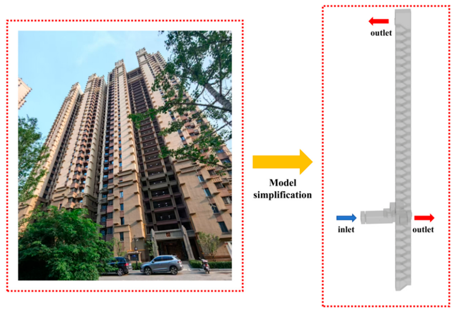
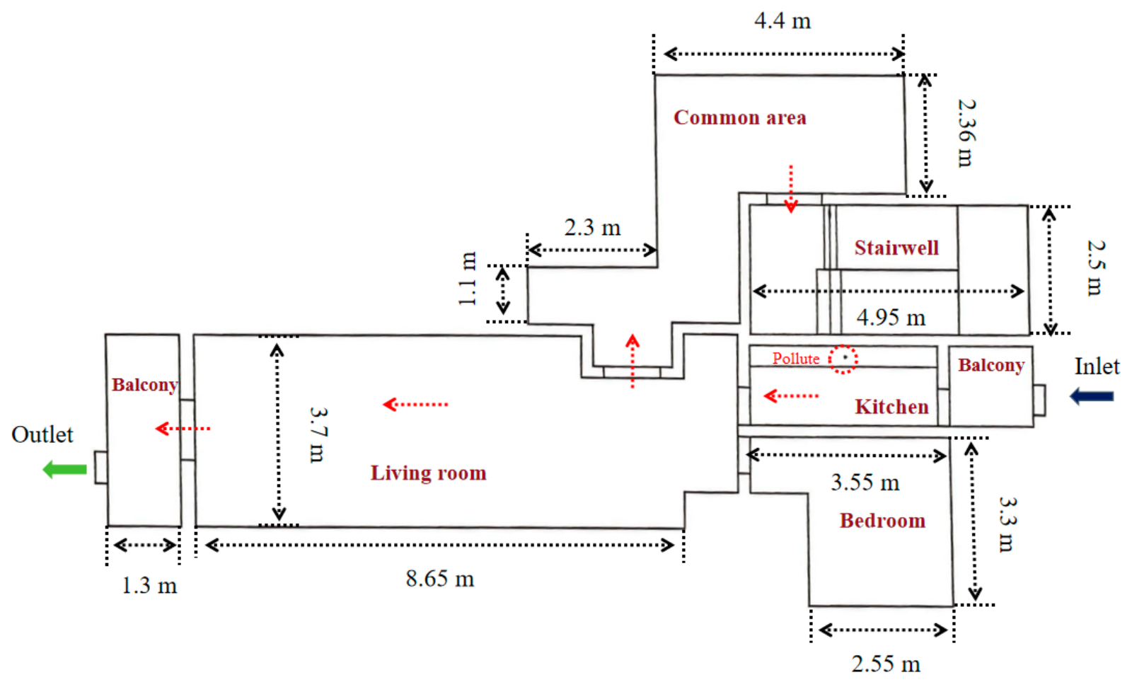
This study focuses on a representative high-rise residential building in Taiyuan (Figure 1), which has overall dimensions of 60.2 m in length (X-axis), 20.3 m in width (Y-axis), and 107 m in height (Z-axis). The floor height is 2.75 m. To facilitate a comprehensive analysis of pollutant dispersion in public areas within the building, the structural components were simplified in the computational model. The model explicitly includes the following features: (1) stairwells, (2) interconnected building zones, and (3) individual dwelling units. A steady pollutant emission was assumed from the center of the living room floor in a certain household. The emission source was modeled as a square opening measuring 0.2 m × 0.2 m, yielding an area of 0.04 m². The simulation domain includes the isolated building only. Neither the external wind field nor surrounding buildings are modeled. The window-velocity condition is a local inflow measured at the source-floor balcony, not a resolved façade pressure field from an atmospheric boundary layer. The simplified airflow diffusion paths and dimensions are shown in Figure 2. For this study, CH₄ and CO₂ were selected as representative gaseous pollutants with buoyant and dense characteristics, respectively. The source conditions were set as follows. The temperature was 20 °C, a typical indoor temperature in winter. The pollutant was released perpendicular to the opening, outward. The species fraction at the source outlet was assumed to be 1 (pure pollutant). The mass flow rate was set to 20 μg/s [22], a value chosen primarily for relative trend comparison across cases rather than to replicate an actual emission rate.

2.2. Experimental Measurement

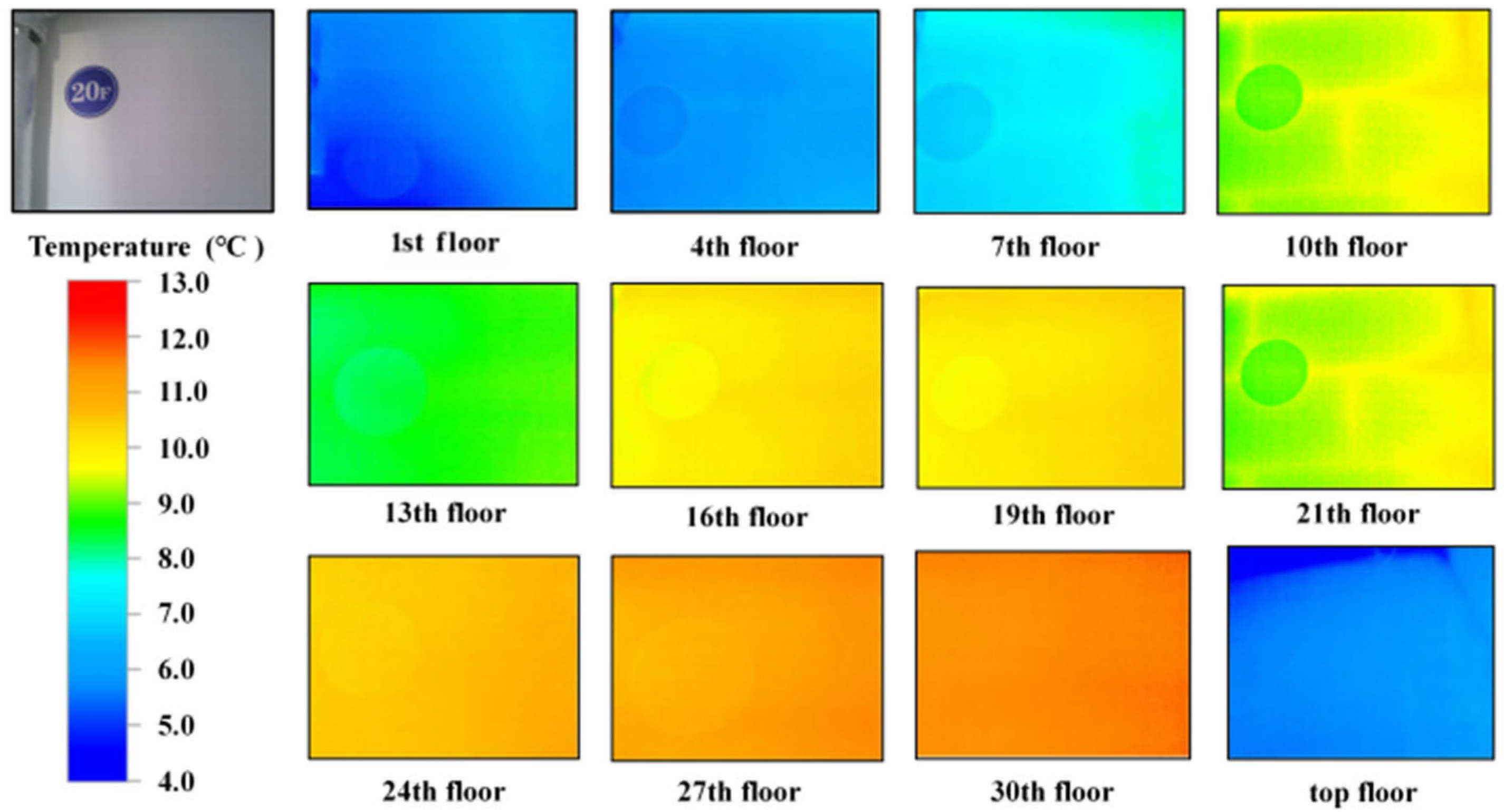
The on-site measurement of wall surface temperatures within the stairwell was conducted using a Testo 872 (Testo SE & Co. KGaA, Titisee-Neustadt, Germany) thermal imager. This instrument has a thermal sensitivity of 0.05 °C and is factory calibrated. The obtained average wall surface temperature data were subsequently applied as boundary conditions in the numerical simulations. The measurement procedure began on the ground floor, with thermal images captured at consistent heights on each successive floor. The measurements were carried out on the morning of 6 December 2024. The outdoor weather was clear with a temperature of about 0 °C. The indoor heating was on. For each wall on each floor, three readings were taken and averaged. The emissivity of the thermal imager was set to 0.95 (the wall surface is concrete). The distance from the imager to the wall was about 1.5 m. After obtaining the average temperatures for the east, west, south, and north walls on each floor, the values were plotted against floor height. A cubic polynomial was then fitted to obtain the temperature–height relationship. A selection of the representative measurement results is presented in Figure 3.

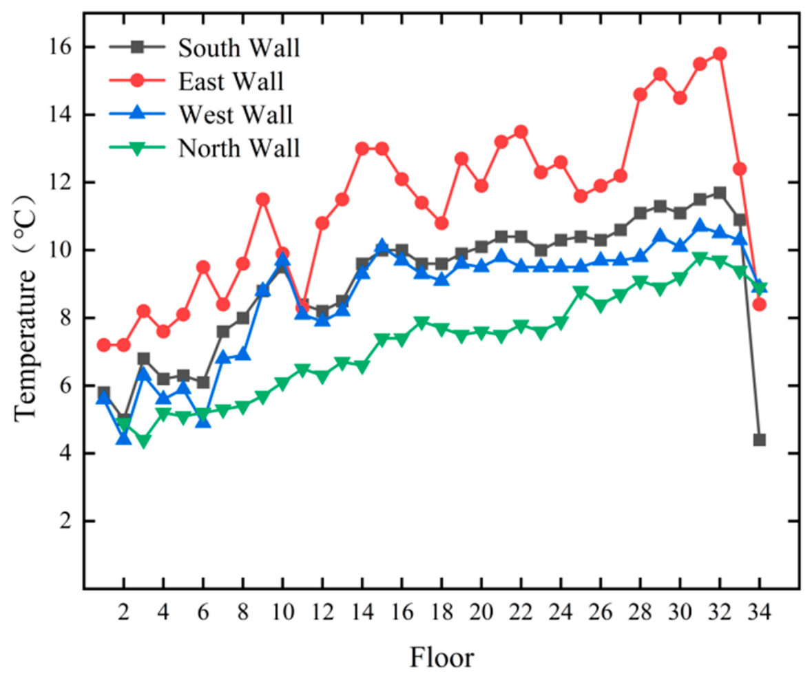
Figure 4 shows the variation in the measured average wall surface temperature as a function of floor height. The temperature exhibits an initial increase followed by a decrease with elevation, consistent with typical winter chimney effect behavior. To mathematically represent this temperature distribution more accurately, a polynomial fitting method was applied. This enabled the derivation of mathematical expressions describing the vertical temperature profiles for the east, west, south, and north walls of the stairwell, as summarized in

Table 2. Fitting formulas for wall surface temperature.

Direction	Formulae	R2	RMSE
East wall	6.59 + 0.28z − 0.0047z2 + 3.07 × 10−5z3	0.82	1.01
West wall	6.01 + 0.29z − 0.0049z2 + 3.20 × 10−5z3	0.86	0.43
South wall	5.06 + 0.22z − 0.0032z2 + 1.75 × 10−5z3	0.93	0.22
North wall	4.72 + 0.093z − 8.3 × 10−4z2 + 5.2 × 10−6z3	0.96	0.1

Note: z denotes floor height (m); valid range 0 to 107 m.

. Simultaneously, wind speed measurements were repeated three times at the balcony window of the source-floor room (10th floor) using a TSI 9535 (TSI 9535 (TSI Incorporated, Shoreview, MN, USA) handheld anemometer (accuracy ±3%, resolution <0.01 m/s, factory calibrated). Three 2-min averaged values were recorded: 0.89 m/s (11:00), 1.11 m/s (14:00), and 0.95 m/s (17:00). The overall average was 0.98 m/s, rounded to 1.0 m/s, which was used as the window velocity inlet in the simulations.

The field measurements had several limitations. First, wall temperatures were measured only on one winter day. Seasonal and daily variations were not considered. Second, wind speed was recorded at only one window for two minutes. This can only represent the local wind speed at that window at that time. It cannot reflect the actual wind pressure distribution on the building facade. Third, no pollutant concentrations were measured in the field. Therefore, the measured data were only used for temperature validation, not for direct validation of the pollutant dispersion results.

2.3. Numerical Simulation

2.3.1. Numerical Model and Boundary Conditions

To simulate fluid flow and the diffusion of pollutants, commonly employed mathematical models include the standard k-ε model, RNG k-ε model, and Realizable k-ε model, among others [23,24,25,26]. Tominaga and Stathopoulos [25] compared four turbulence models—standard k-ε (SKE), RNG k-ε (RNG), Realizable k-ε (RLZ), and shear stress transport (SST) k-ω—using computational fluid dynamics (CFD). Their findings demonstrated that Reynolds-Averaged Navier–Stokes (RANS) simulations effectively capture the influence of plume buoyancy on mean concentration distributions, confirming the reliability of such approaches for modeling buoyancy-driven pollutant dispersion. The standard k-ε model in ANSYS 2023 Fluent was used to solve the transient flow field. The mixture density is computed using the incompressible ideal gas law, which depends on local temperature and species mass fractions (operating pressure fixed at 101,325 Pa). The species transport model tracks the mass fractions of CH₄, CO₂, and air. The gravitational term (ρg) in the momentum equation thus accounts for both thermal buoyancy (from temperature differences) and species-driven buoyancy (e.g., CH₄ lighter than air, CO₂ heavier). Gravity was set to 9.81 m/s² in the downward direction. The pressure–velocity coupling was handled by the SIMPLEC scheme. Pressure discretization used the second order scheme, and the gradient was computed using the least squares cell-based method. Momentum, energy, and air species were discretized with the second order upwind scheme. Turbulent kinetic energy and its dissipation rate used the first order upwind scheme. A fixed time step of 1 s was used, with a total of 7200 time steps. No formal time-step sensitivity analysis was performed. Time integration was first-order implicit. Under-relaxation factors were 0.7 for pressure and momentum, and 0.8 for turbulent kinetic energy and dissipation rate. Other quantities (density, body forces, turbulent viscosity, energy) retained the default value of 1.0. Each time step allowed up to 20 iterations. Convergence criteria were set as residuals below 10⁻⁴ for continuity, velocity, k, and ε, and below 10⁻⁶ for energy and species.

For the velocity inlet at the balcony window, the turbulence intensity was set to 5%, and the hydraulic diameter was 0.45 m (based on the window opening). The wall temperature was defined using height-dependent fitting formulas derived from measured wall temperatures (Table 2), which were imported into the model via user-defined functions (UDF). See Appendix A for the UDF code All walls were no-slip walls. The balcony window was specified as a velocity inlet, with the incoming wind speed and temperature set to the measured values of 1 m/s and 0 °C, respectively. The kitchen window and the roof staircase door were set as pressure outlets. The backflow temperature was 0 °C (matching outdoor conditions), and backflow turbulence parameters were the same as those at the inlet. The pollutant release port was treated as a mass flow inlet, with a release rate of 20 μg/s. A complete summary of boundary conditions and initial conditions is provided in

Table 3. Boundary conditions and initial state for the CFD simulation.

Boundary Name	Boundary Type	Specified Parameters
Balcony window	Velocity Inlet	Velocity: 1 m/s; Temperature: 0 °C; Turbulence Intensity: 5%; Hydraulic Diameter: 0.45 m; Species: Air = 1, CH4/CO2 = 0
Kitchen windows	Pressure Outlet	Gauge Pressure: 0 Pa; Backflow Temperature: 0 °C; Backflow Turbulence Intensity: 5%; Backflow Hydraulic Diameter: 0.45 m; Backflow Species: Air = 1, Pollutant = 0
Roof staircase door	Pressure Outlet	Same parameters as the kitchen window outlets
Pollutant release port	Mass Flow Inlet	Mass Flow Rate: 20 μg/s (2 × 10−8 kg/s), Species Mass Fraction: 1 (Pure CH4 or CO2), Temperature: 20 °C (indoor condition), Flow Direction: Normal to boundary
Stairwell walls (East, West, South, North)	Wall (No-slip)	Thermal Condition: Temperature profile defined by UDF (height-dependent cubic polynomial from Table 2) Wall Condition: No-slip, zero species flux
Interior partitions (Internal walls, floors, ceilings,)	Wall (No-slip)	Thermal Condition: 20 °C Wall Condition: No-slip, zero species flux
Initial conditions (t = 0 s)	—	Velocity: 0 m/s; Temperature: 0 °C (uniform); Gauge Pressure: 0 Pa; Species: Air = 1, CH4/CO2 = 0; Turbulent Kinetic Energy: 0.0035 m2/s2; Turbulent Dissipation Rate: 0.00881 m2/s3

. CH₄ and CO₂ were selected as the representative lightweight and dense pollutants, respectively, for separate diffusion simulations. The species transport model was used without chemical reactions. The resulting source velocities are approximately 7.5 × 10⁻⁷ m/s for CH₄ and 2.7 × 10⁻⁷ m/s for CO₂, which are negligible compared to the window inlet (1 m/s). The mass diffusivities were 2.1 × 10⁻⁵ m²/s for CH₄ in air and 1.6 × 10⁻⁵ m²/s for CO₂ in air. Material properties (density, specific heat, viscosity, thermal conductivity) for air, CH₄ and CO₂ were taken from the Fluent default database. See

Table 4. Thermophysical properties of working fluids.

Property	Air	CH4	CO2
Molecular weight, M (kg/kmol)	28.97	16.04	44.01
Density, ρ (kg/m3)	1.225	0.667	1.830
Specific heat, Cp (J/(kg·K))	1006.43	Piecewise-polynomial	Piecewise-polynomial
Thermal conductivity, k (W/(m·K))	0.0242	0.0336	0.0165
Dynamic viscosity, μ (kg/(m·s))	1.789 × 10−5	1.10 × 10−5	1.47 × 10−5
Mass diffusivity in air, D (m2/s)	–	2.10 × 10−5	1.60 × 10−5

for a complete list of these properties.

2.3.2. Mesh Generation

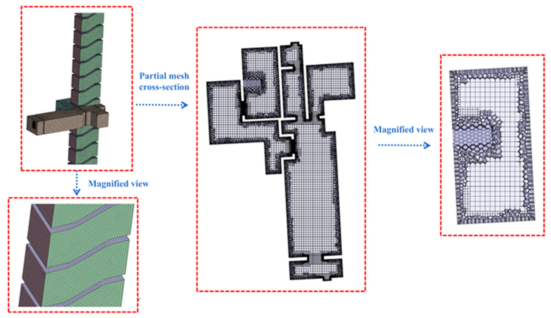
In this study, Fluent Meshing was used to generate the mesh. The mesh type is poly-hexcore, a hybrid of hexahedral core and polyhedral cells. Polyhedral cells are placed near walls to better capture geometric details. Hexahedral cells are used in regions away from walls to improve computational efficiency. This combination balances accuracy and speed.

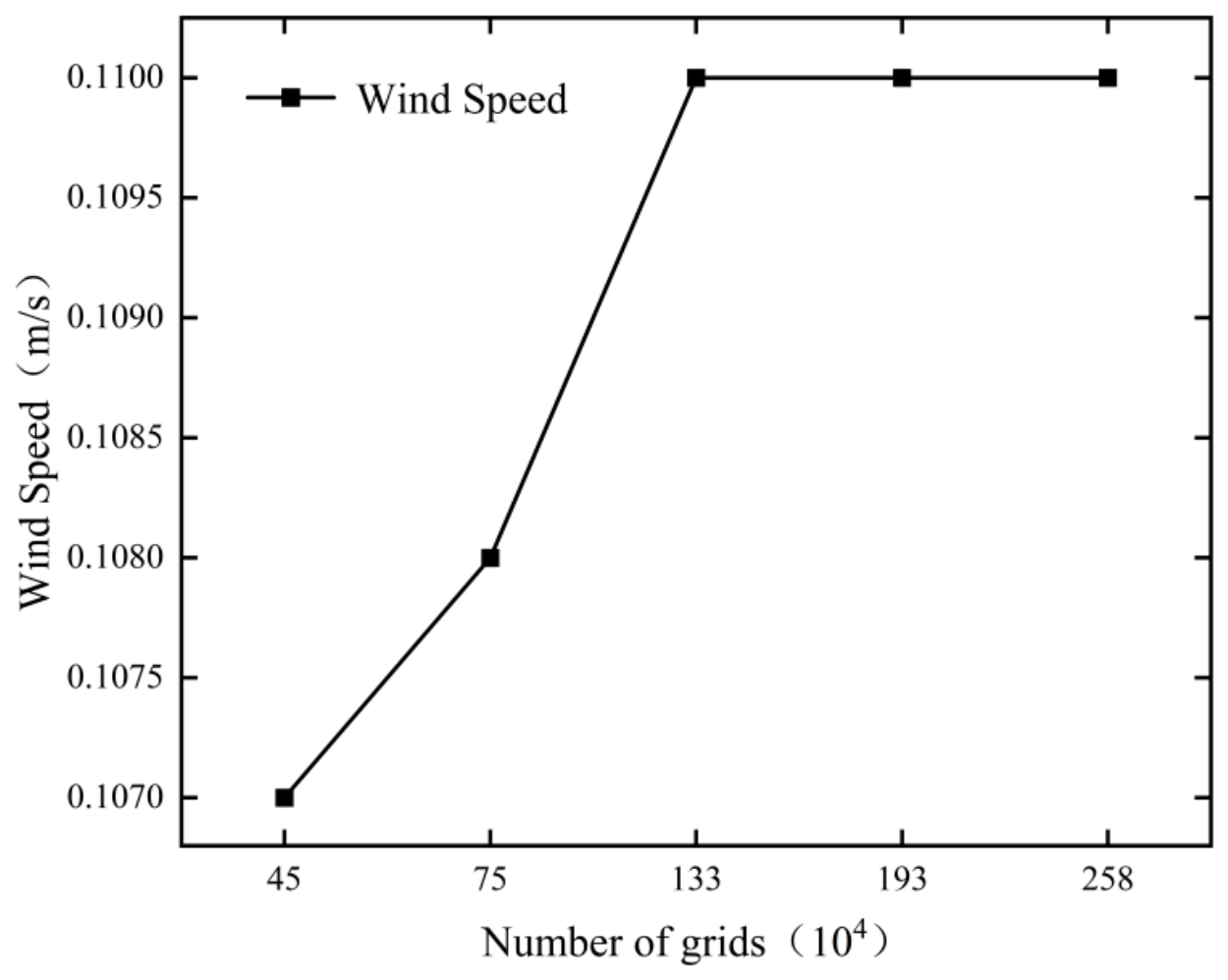
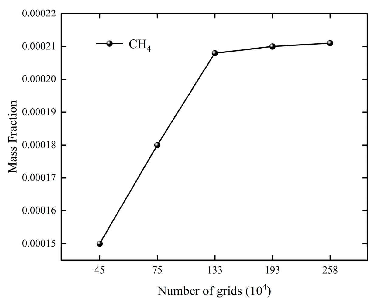
To mitigate the influence of mesh quality on simulation results, velocity values at plane z = 76.2 m on the 26th floor of the stairwell were compared for mesh counts of 0.45 million, 0.75 million, 1.33 million, 1.93 million, and 2.58 million. As shown in Figure 5, at a mesh count of 1.33 million, the velocity deviated by less than 1% from the values obtained with 1.93 million and 2.58 million. A similar mesh independence check was performed for CH₄ concentration on the source floor (1.5 m above the floor, z = 28.9 m), as presented in Figure 6. At 1.33 million cells, the CH₄ concentration differed by less than 3% from the values at 1.93 million and 2.58 million. Consequently, a mesh with 1.33 million elements was selected for subsequent calculations, as shown in Figure 7. The average orthogonal quality was 0.921, the average skewness was 0.069, the maximum skewness was 0.61 and the average aspect ratio was 3.36. The minimum orthogonal quality (0.154) occurred only in a few local regions, and the overall mesh quality is acceptable for engineering CFD simulations. Near-wall treatment uses the standard wall function. The area-weighted average y+ on the main vertical walls is 20.7, with individual values ranging from 14.1 to 27.2. Although the minimum y+ is slightly below the recommended lower bound of 15 for standard wall functions, the average value is acceptable. It should be noted that the grid independence verification was based only on local velocity and concentration values. More comprehensive metrics, such as floor-averaged concentration or mass flow balance across openings, were not examined. The selected grid is considered adequate for the comparative trend analysis in this study, and this limitation is acknowledged. The overall mesh size was constrained within the range of 0.01–0.25 m, and a multi-level local mesh refinement strategy was employed: a refined mesh with a size of 0.01 m was implemented at the pollutant source release port; the mesh size for complex geometric structures such as door and window frames was set to 0.05 m; and the mesh size for other wall regions was 0.2 m. Additionally, three layers of boundary layer meshes were constructed adjacent to the walls to capture the near-wall flow boundary layer effect.

2.4. Experimental Verification

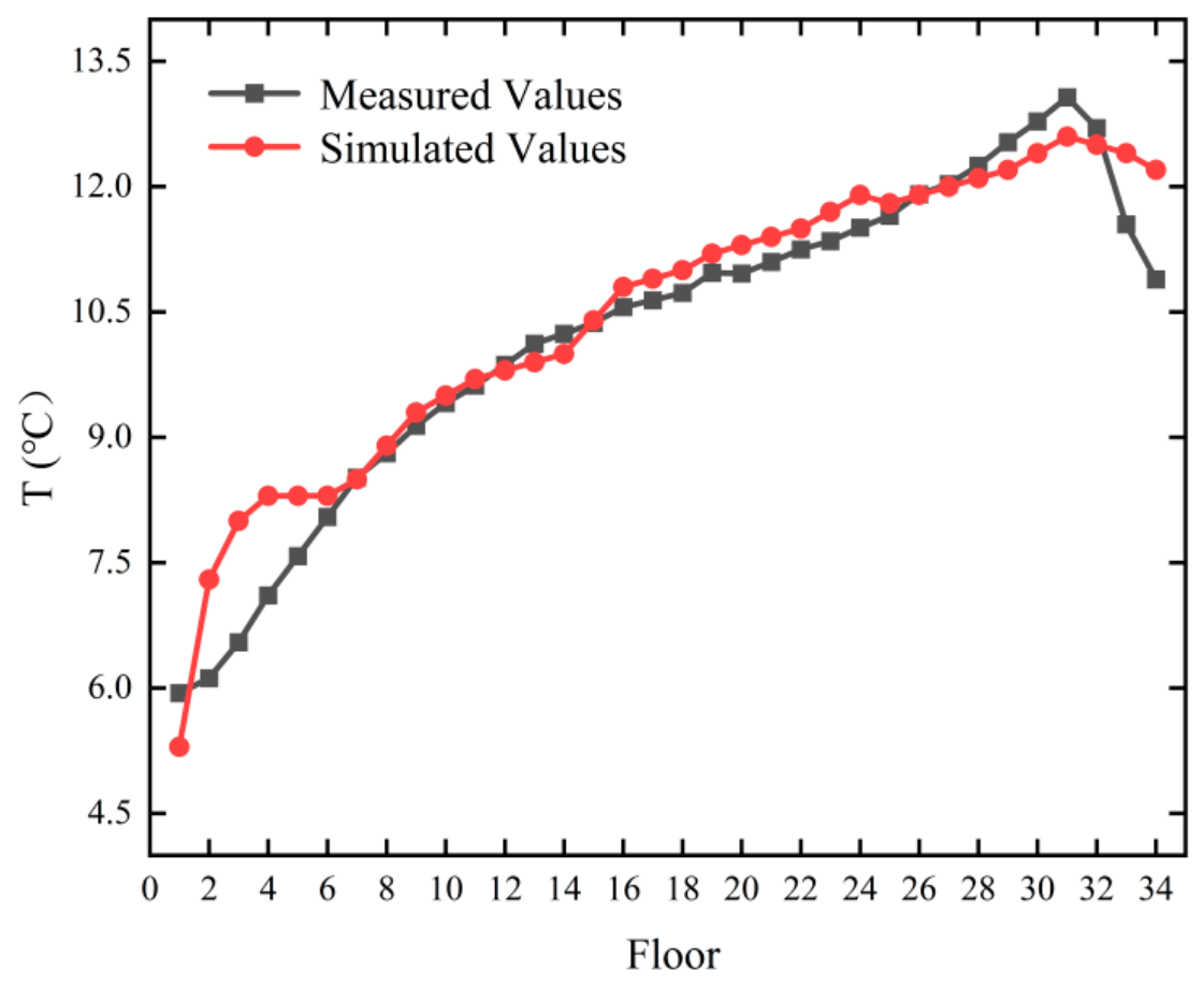
To validate the numerical simulation model and wall boundary conditions, real-time air temperature monitoring in the stairwell was performed using a Fluke 971 (Fluke 971 (Fluke Corporation, Everett, WA, USA) temperature and humidity meter. This instrument has a resolution of 0.1 °C and an accuracy of ±0.5 °C. A comparison between simulated and measured temperatures from the 1st to 34th floor is shown in Figure 8. The results show good overall agreement. The measured temperature increases from 5.3 °C at the 1st floor to 12.6 °C near the 31st floor, then slightly decreases to 12.2 °C at the 34th floor. The simulation captures this trend well. The mean absolute error (MAE) between simulated and measured temperatures is 0.38 °C, and the root mean square error (RMSE) is 0.54 °C. The maximum absolute deviation occurs on the 3rd floor (1.45 °C). The good temperature agreement indicates that the thermal boundary conditions and stack effect are realistically reproduced; however, the pollutant dispersion predictions have not been directly validated experimentally. The CH₄/CO₂ transport results should therefore be interpreted as numerical predictions under the assumed model and boundary conditions, pending future full-scale tracer gas experiments.

3. Results and Discussion

3.1. Vertical Diffusion Characteristics of CH₄ and CO₂ in Buildings Under Thermal Pressure Conditions

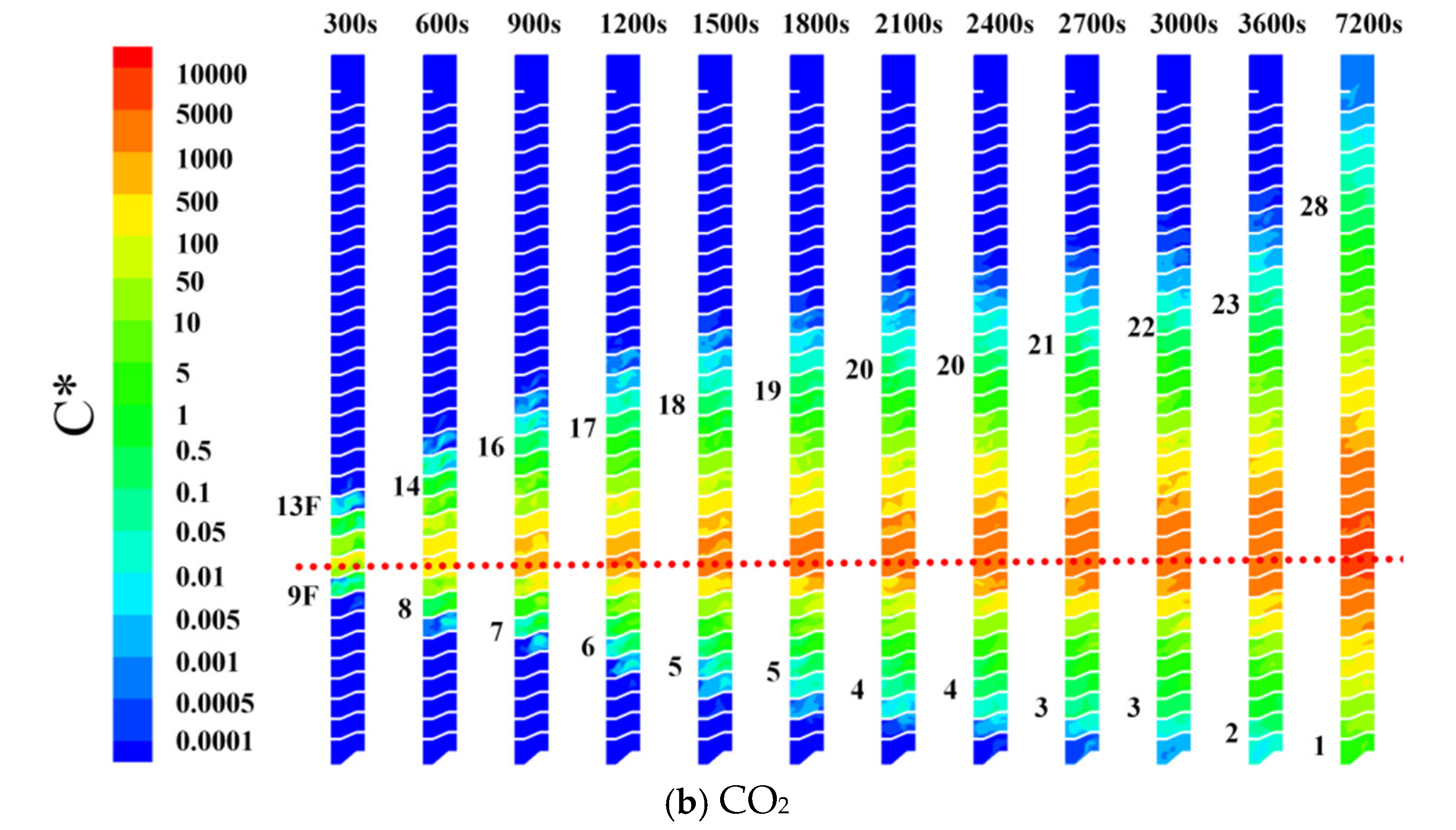
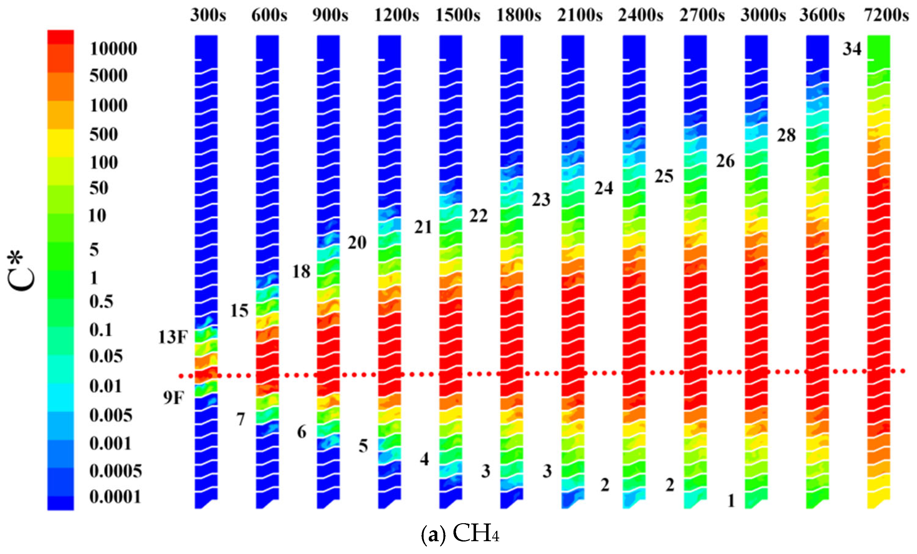
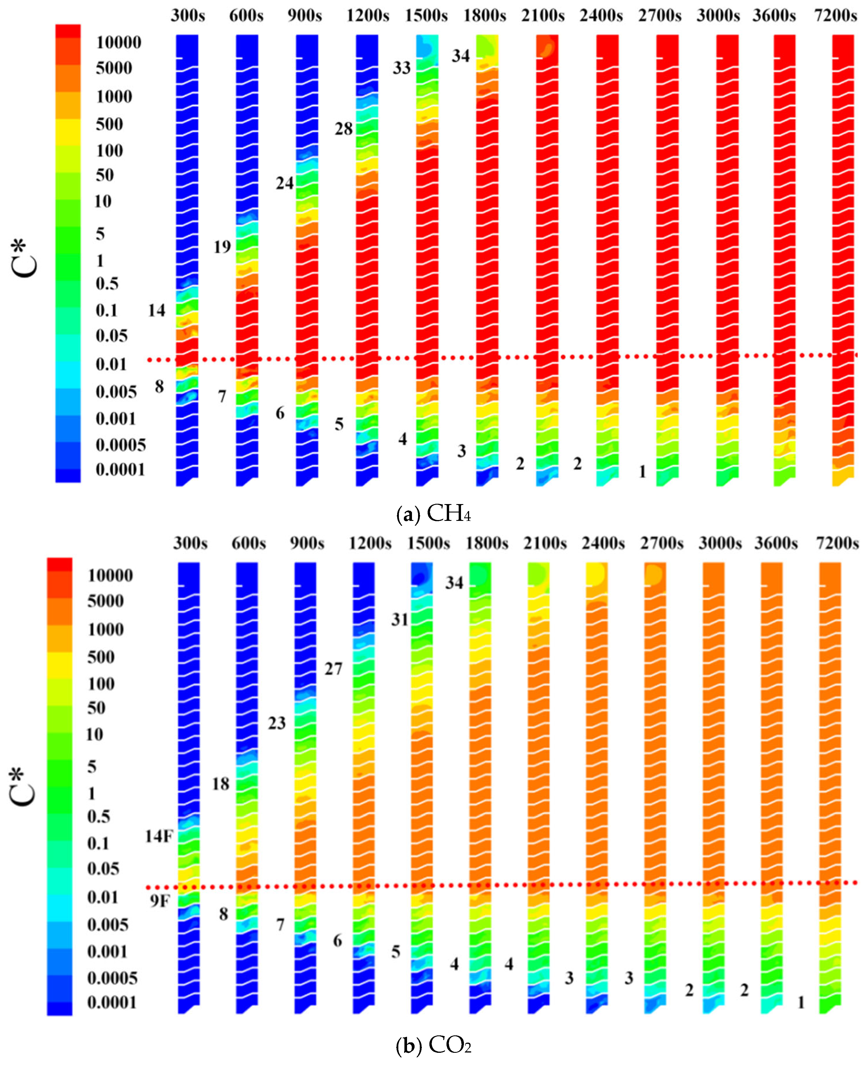
Figure 9a,b illustrate the spatiotemporal distribution of vertical cross-sectional concentrations of the buoyant pollutant CH₄ and the dense pollutant CO₂ in the stairwell under thermal pressure conditions.

The scaled mass fraction C* is defined as:

$$\mathrm{C}*={\displaystyle \frac{\mathrm{C}}{\mathrm{k}}}$$

where C is the local mass fraction of the pollutant (kg/kg), and k = 2 × 10⁻⁸ is a constant derived from the source mass flow rate (20 μg/s). This definition provides a uniform scaling factor for all simulation cases, enabling consistent comparison of pollutant distributions under different driving conditions (thermal pressure, window-velocity, and their coupling). The absolute value of C* does not represent a physically rigorous scaled mass fraction; it serves only as a relative index for comparative analysis. As shown in Figure 9a, CH₄ diffusion under thermal pressure is asymmetric: upward is faster than downward. In the first 900 s, the upward rate is 2–3 floors/300 s, driven by thermal buoyancy; after 900 s, it drops to 1 floor/300 s and reaches the 28th floor at 3600 s. Downward diffusion is slower (1 floor/300 s on average, occasionally 2 floors/300 s from 300–600 s), and further decreases to 0.5 floors/300 s after 1800 s due to the antagonism between buoyancy (upward) and gravity (downward). Figure 9b shows similar but weaker behavior for CO₂. At 300 s, CO₂ reaches floors 9–12 (one floor less than CH₄). Its upward rate remains 2–3 floors/300 s until 900 s, then declines to 1 floor/300 s. By 3600 s, CO₂ covers four fewer floors upward than CH₄. Downward rates are 1 floor/300 s (t < 1800 s) and 0.5 floors/300 s thereafter, consistently slower than CH₄. The detailed front positions of both pollutants at selected times are listed in

Table 5. Time-resolved upward and downward front floors of CH₄ and CO₂ under thermal pressure.

Time (s)	CH4 (Floor)		CO2 (Floor)
	Upward	Downward	Upward	Downward
300	13	9	12	9
600	15	7	14	8
900	18	6	16	7
1200	20	5	18	6
1500	21	4	19	6
1800	22	3	20	5
2100	23	3	21	5
2400	24	2	22	4
2700	25	2	23	4
3000	26	1	24	3
3600	28	1	26	3
7200	34	1	30	3

.

For CH₄ (lighter than air), the inherent buoyancy is upward and aligns with thermal buoyancy. Both forces cooperate to drive CH₄ upward. The steep concentration gradient near the source also provides a diffusive push from high to low concentration. Above the source floor, these three drivers are synergistic, resulting in an initial upward rate of 2–3 floors per 300 s. For CO₂ (denser than air), the inherent buoyancy acts downward, opposing thermal buoyancy. Its concentration gradient is also weaker because upward spread is limited. Consequently, the net upward driving force is smaller, and upward diffusion is slower. Below the source floor, the concentration gradient drives pollutants from the source (high concentration) to lower floors. Thermal buoyancy, however, acts upward and opposes downward transport. Gravity is already accounted for in the inherent buoyancy term. For CH₄, the steep concentration gradient overcomes the opposing thermal buoyancy, giving a downward rate of about 1 floor per 300 s. For CO₂, the concentration gradient is much weaker, so its downward rate is not higher than that of CH₄. This explains why CO₂ does not descend faster than CH₄ despite being heavier. Upward diffusion of CH₄ benefits from three aligned forces (thermal buoyancy, inherent lightness, and concentration gradient), whereas CO₂ suffers from opposing forces and a weaker gradient. Downward, the concentration gradient dominates, and CH₄ again outperforms CO₂ due to its steeper gradient.

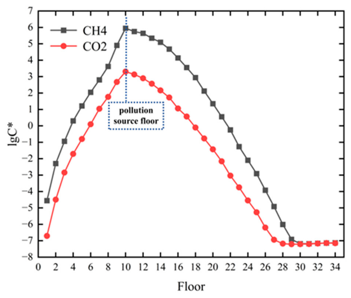
The scaled mass fraction distributions of CO₂ and CH₄ at t = 1800 s under thermal pressure conditions on each floor are presented on a logarithmic scale in Figure 10. For ease of display, the vertical coordinate is the logarithm of the scaled mass fraction. As shown in Figure 10, the distributions of both CH₄ and CO₂ initially increase, then decrease, and eventually stabilize with increasing floor height. However, notable differences are observed in peak intensity, distribution range, and attenuation characteristics. The maximum concentrations of both pollutants occur on the pollution source floor (10th floor), with the peak concentration of CH₄ reaching 10⁶, compared to only 10³ for CO₂—a difference of three orders of magnitude. This indicates a significantly stronger aggregation effect of CH₄ near the pollution source. Using a scaled mass fraction threshold of 10⁻¹, the affected floors for CH₄ span from the 3rd to the 22nd, while for CO₂ they range from the 5th to the 19th, indicating a stronger spatial diffusion capacity of CH₄. It should be noted that the affected-floor range depends on the chosen threshold, and a formal threshold sensitivity analysis was not performed in this study. Except for the top floors (29–34), the concentration level of CH₄ is approximately two orders of magnitude higher than that of CO₂ on all other floors. In the top floor region, the concentrations of both pollutants converge to similar values, suggesting the formation of a uniform low-concentration field in this area by t = 1800 s under sustained thermal pressure. The diffusion characteristics of CH₄ throughout the building—particularly its rapid diffusion above the pollution source floor—corresponds quantitatively to its higher diffusion rate observed in Figure 9. This further confirms that buoyant pollutants possess enhanced migration capacity under thermal pressure. The difference fundamentally stems from density-induced variations in thermal buoyancy effects, which enable buoyant species to exhibit superior long-distance transport capability.

3.2. Vertical Diffusion Characteristics of CH₄ and CO₂ in Buildings Under Window Velocity Conditions

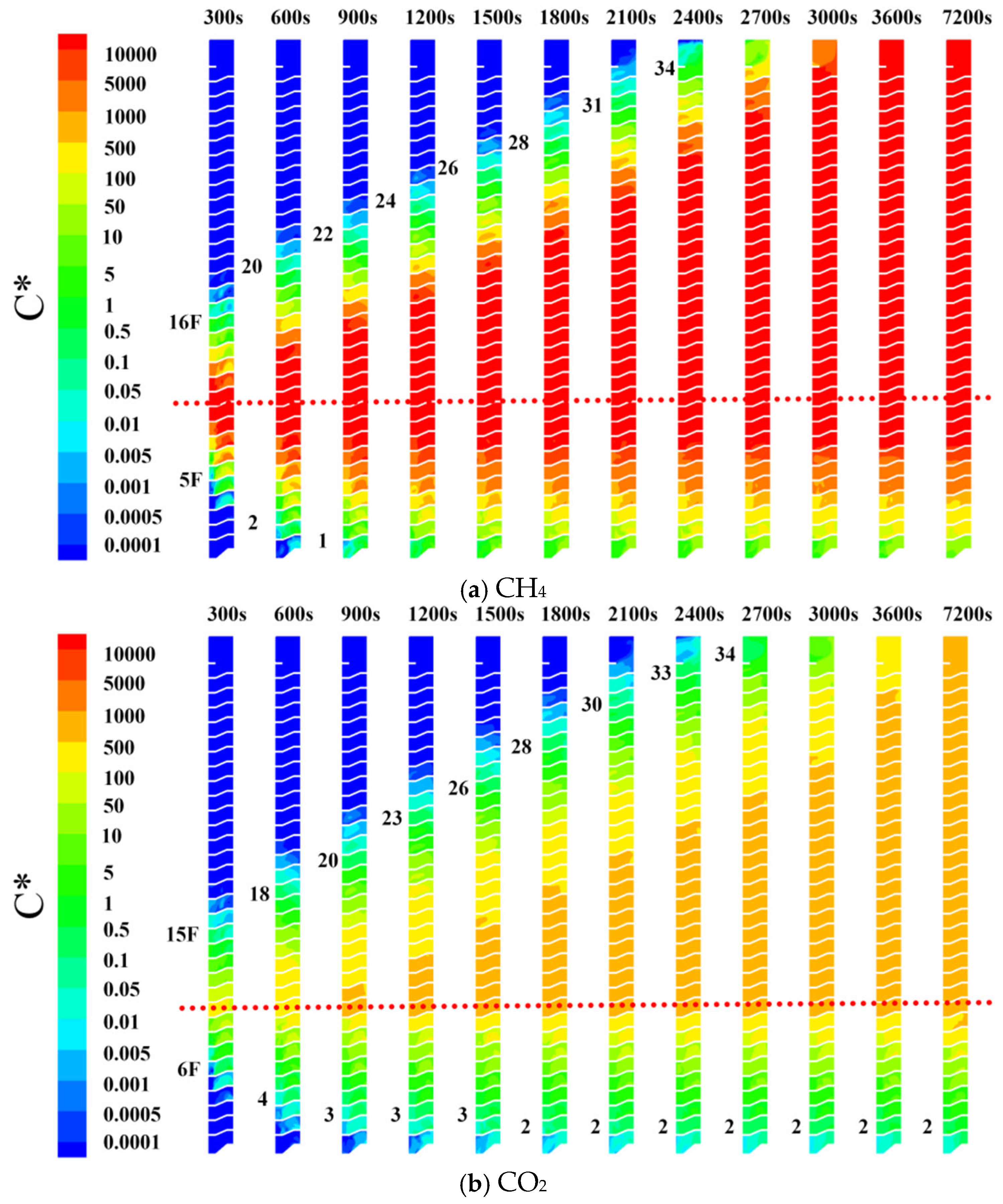
Figure 11a,b present the scaled mass fraction spatiotemporal distribution of buoyant pollutant CH₄ and dense pollutant CO₂ in the vertical section of the stairwell under window velocity conditions. As shown in Figure 11, CH₄ reaches floors 5 to 16 by t = 300 s. Above the pollution source floor, it continues to spread upward at a constant rate of 2–4 floors per 300 s, attaining the top floor by t = 2400 s. Below the source floor, however, CH₄ reaches the bottom floor in only 900 s. Compared to the thermal pressure condition shown in Figure 9a, CH₄ exhibits a faster diffusion rate under window velocity conditions without showing any deceleration. As shown in Figure 11b, the diffusion behavior of CO₂ differs markedly from that of CH₄. At t = 300 s, CO₂ has only reached floors 6–15, covering a range two floors smaller than that of CH₄. Its upward diffusion proceeds at a rate of 2–3 floors per 300 s, reaching the top floor by t = 2700 s. In contrast, downward diffusion slows considerably after attaining the 3rd floor (t = 900 s), and the bottom floor is not reached until t = 7200 s. The detailed front positions at selected times are listed in

Table 6. Time-resolved upward and downward front floors of CH₄ and CO₂ under window velocity.

Time (s)	CH4 (Floor)		CO2 (Floor)
	Upward	Downward	Upward	Downward
300	16	5	15	6
600	20	2	18	4
900	22	1	20	3
1200	24	1	23	3
1500	26	1	26	3
1800	28	1	28	2
2100	31	1	30	2
2400	34	1	33	2
2700	34	1	34	2
3000	34	1	34	2
3600	34	1	34	2
7200	34	1	34	2

. Analysis of the concentration distributions reveals distinct spatial differences between the two pollutants. CH₄ forms high-concentration zones (scaled mass fraction > 10⁴) both above and below the pollution source floor, exhibiting a symmetrical vertical profile. In contrast, the maximum concentration of CO₂ remains confined to the region above the source floor, reaching only 10², while its downward diffusion is significantly slower.

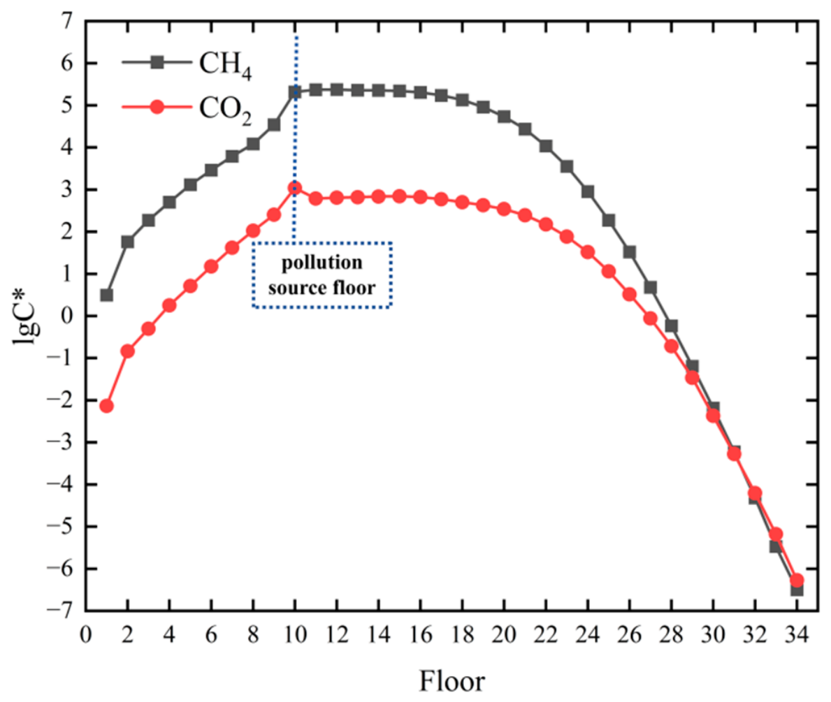
The logarithmic scaled mass fraction distributions of CO₂ and CH₄ on each floor at t = 1800 s are shown in Figure 12. As illustrated, both pollutants have diffused to areas above and below the pollution source floor. Within ten floors above and below the pollution source floor (10th floor), the scaled mass fraction of CH₄ remains consistently two orders of magnitude greater than that of CO₂. This difference, however, gradually diminishes above the 20th floor. CH₄ diffuses across floors 1 to 28, whereas CO₂ covers two fewer floors below the pollution source floor, failing to reach floors 1 and 2. Given that both the wind inlet and pollution source are situated on the 10th floor, pollutants are transported upward by the vertical airflow and eventually discharged through the roof staircase door. The absence of openings in the lower zone of the pollution source floor leads to pollutant accumulation in this region. Furthermore, owing to the stronger long-distance transport capacity of buoyant pollutants, CH₄ exhibits higher scaled mass fraction throughout the stairwell, exceeding those of CO₂ by approximately 2 to 4 orders of magnitude. This phenomenon suggests that, in window velocity-dominated transport processes, pollutant dispersion is jointly controlled by pollutant density, concentration gradient, and airflow direction.

3.3. Vertical Diffusion Characteristics of CH₄ and CO₂ in Buildings Under Wind–Thermal Coupling Conditions

Figure 13 shows the spatiotemporal distribution of scaled mass fraction of buoyant CH₄ and dense CO₂ in the stairwell vertical section under wind–thermal coupling. As seen in Figure 13a, the CH₄ concentration exhibits clear stratified diffusion centered at the source floor. Above the source floor, CH₄ diffuses upward at a rate of 4–5 floors per 300 s under wind–thermal coupling. To quantify the enhancement, we used the 28th floor as a reference—the floor reached by CH₄ after 3600 s under thermal pressure alone. The time required to reach this floor is 3600 s (thermal pressure), 1800 s (window velocity), and 1200 s (coupling). Thus, the upward diffusion rate under coupling is three times that under thermal pressure (200% faster) and 1.5 times that under the window-velocity condition (50% faster). For detailed comparisons, see

Table 7. Time-resolved upward and downward front floors of CH₄ and CO₂ under wind–thermal coupling condition.

Time (s)	CH4 (Floor)		CO2 (Floor)
	Upward	Downward	Upward	Downward
300	14	8	14	9
600	19	7	18	8
900	24	6	23	7
1200	28	5	27	6
1500	33	4	31	5
1800	34	3	34	4
2100	34	2	34	4
2400	34	2	34	3
2700	34	1	34	3
3000	34	1	34	2
3600	34	1	34	2
7200	34	1	34	1

and

Table 8. Summary of vertical diffusion characteristics for CH₄ and CO₂ under three driving conditions.

Pollutant	Condition	Arrival at 28th (s)	Peak C*	Affected Floors (7200 s)	Upward Rate (Floors/300 s)	Downward Rate (Floors/300 s)
CH4	Thermal	3600	~106	1–34	1–3	0–2
	Window velocity	2400	~105	1–28	2–6	0–1
	Coupling	1200	~105	1–34	4–5	0–1
CO2	Thermal	>3600	~103	2–34	0.5–3	0–1
	Window velocity	2700	~103	1–34	1–5	0–4
	Coupling	1800	~103	1–34	4–5	0–1

. From the concentration distribution, except at the initial stage (t = 300 s), the number of floors where CH₄ reaches the maximum pollution level (10⁴) in this region exceeds that under window velocity alone. By t = 2100 s, the pollutant concentration on all floors above the pollution source has stabilized at the maximum level. Under the combined driving forces, CO₂ exhibits weaker migration capacity than CH₄. Above the pollution source floor, its diffusion behavior resembles that under window velocity-dominated conditions; below, it approximates the pattern observed under thermal pressure-dominated conditions. CO₂ reaches the top floor by t = 1800 s, diffusing at a rate of 3–5 floors per 300 s. However, it requires an additional 600 s for all floors to attain the maximum pollutant level (above 10³) compared to CH₄, confirming the influence of density on pollutant diffusion. Below the pollution source floor, the diffusion of both pollutants slows significantly.

The diffusion rate of CH₄ decreases to approximately 1 floor per 300 s, and it does not reach the bottom floor until t = 2700 s—1800 s slower than under window velocity conditions—exhibiting behavior similar to that under thermal pressure. In comparison, CO₂ diffuses to the 4th floor at a rate of 1 floor per 300 s for t < 1800 s, then slows further, only reaching the bottom floor by t = 7200 s. This difference in diffusion behavior stems from distinct dominant driving mechanisms. Above the pollution source floor, window velocity-induced forced convection acts as the primary driver of pollutant migration, while thermal buoyancy plays a secondary role. Below the source floor, however, thermal pressure and concentration gradients dominate, with gravity serving as an additional influencing factor.

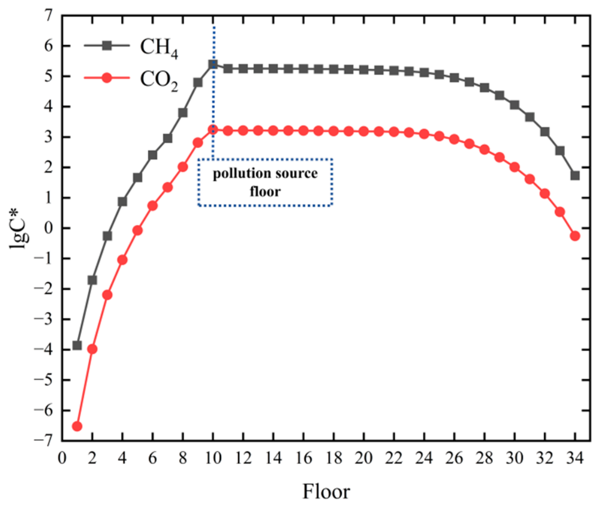
The logarithmic scaled mass fraction distributions of CO₂ and CH₄ at each floor at t = 1800 s under wind–thermal coupling conditions are presented in Figure 14. Below the pollution source floor, the logarithmic scaled mass fraction increases gradually with rising floor height, reaches its maximum at the 10th floor where the pollution source is located, and then decreases slowly. The rate of decrease accelerates significantly beyond the 24th floor. Comparative analysis shows that above the pollution source floor (10th floor), both the diffusion rate and pollutant concentration under wind–thermal coupling conditions exceed those under pure thermal or pure window velocity conditions. This confirms that wind–thermal coupling enhances pollutant diffusion in the region above the source floor. The concentrations of both pollutants in the upper region above the pollution source are 3–4 orders of magnitude lower than those at the pollution source floor, which is highly consistent with the research findings of Mao [20]. In terms of differences between pollutant types, the concentration magnitudes of CH₄ and CO₂ consistently differ by two orders of magnitude. Specifically, the maximum concentration magnitude of CO₂ at the pollution source floor (10th floor) is 10³, while that of CH₄ is 10⁵. This difference arises mainly from their different densities and molecular diffusivities: CH₄ is lighter and diffuses faster, which facilitates its upward transport into the stairwell, whereas CO₂ tends to sink and stay in the room.

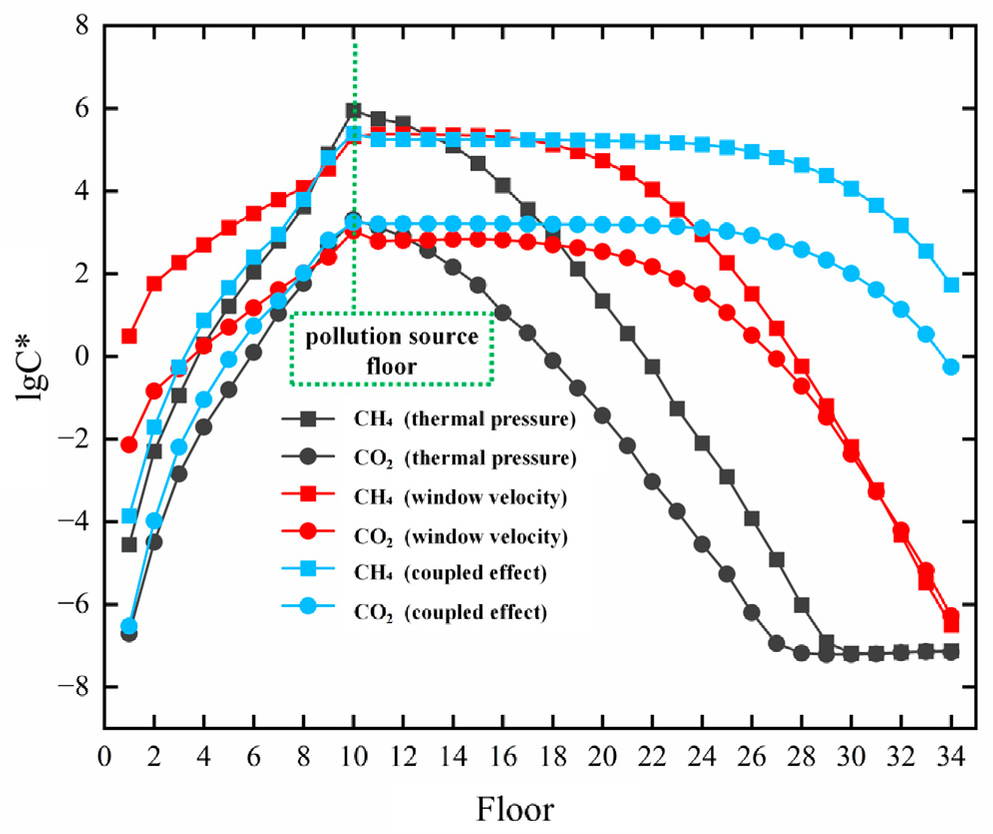
Figure 15 compares the logarithmic scaled mass fraction distributions of CH₄ and CO₂ on each floor under the three conditions at t = 1800 s. In all conditions, the simulated CH₄ shows a wider diffusion range and higher rate than CO₂. Under the present CFD setup (standard k-ε model, simplified window velocity inlet, and incompressible ideal gas law for mixture density), this is attributed to the lower density of CH₄, which makes it more responsive to buoyancy and wind, and to its higher molecular diffusivity, which establishes a steeper concentration gradient. The diffusion patterns differ above and below the source floor. Under thermal pressure, the simulated upward diffusion is faster than downward diffusion, producing an asymmetric “fast-up, slow-down” pattern. Under the window velocity condition, the simulated diffusion is nearly symmetric. Under wind–thermal coupling, the simulated upward diffusion rate is the highest (4–5 floors/300 s for CH₄), while the downward diffusion resembles the thermal-pressure case. These simulated trends suggest a hybrid pattern that combines characteristics of both driving mechanisms.

4. Conclusions

This study investigated the vertical diffusion of CH₄ and CO₂ in the stairwell of a specific high-rise residential building in Taiyuan, under three driving conditions (thermal pressure, a measured window-velocity condition, and their coupling). Field-measured wall temperatures and window wind speeds were used as boundary conditions for transient CFD simulations. The following conclusions are drawn within the scope of this specific case (single building, one source floor at the 10th floor, a simplified inflow boundary based on a 2-min wind measurement, and idealized building surroundings):

• Under thermal pressure alone, dispersion is driven by thermal buoyancy and the concentration gradient. The diffusion pattern is asymmetric: upward is faster than downward. For CH₄, the upward rate is initially 2–3 floors/300 s, then slows to 1 floor/300 s; it reaches the 28th floor at 3600 s. The affected floors of CH₄ range from 3 to 22 at t = 1800 s, with a peak scaled mass fraction of 10⁶ at the source floor. CO₂ shows similar but weaker behavior: its upward rate is slower (reaches 26th floor at 3600 s), and its peak concentration is 10³. The weaker downward diffusion of CO₂ is due to its smaller concentration gradient.
• Under the measured window-velocity condition, forced convection dominates, producing a nearly symmetric diffusion pattern. CH₄ spreads upward at 2–4 floors/300 s and reaches the top floor at 2400 s; it descends to the bottom floor in 900 s. CO₂ rises at 2–3 floors/300 s, reaching the top floor at 2700 s, but its downward spread is much slower (bottom floor only at 7200 s). Again, concentration gradient differences explain the slower migration of CO₂.
• Under wind–thermal coupling, the upward region exhibits a combined effect of wind, thermal buoyancy, and concentration gradient, giving CH₄ an upward rate of 4–5 floors/300 s and a top-floor arrival at 1800 s—approximately 200% faster than under thermal pressure and 50% faster than under the window velocity condition. Below the source floor, upward thermal buoyancy counteracts downward wind, so diffusion is dominated by the concentration gradient, behaving similarly to the thermal-pressure case. CO₂ again shows weaker migration (peak concentration about two orders lower than CH₄).

Limitations and generalizability: The results are specific to the studied building, the 10th-floor single source, the simplified inflow boundary (1 m/s measured at one window), and the winter thermal condition. Multi-source scenarios, interactions with surrounding buildings, and different meteorological conditions were not examined. Therefore, the quantitative values (e.g., diffusion rates, arrival times) should not be directly extrapolated to other buildings or conditions without further validation. However, the observed mechanistic trends—such as the synergistic enhancement of upward diffusion under coupling and the dominant role of the concentration gradient in downward transport—may provide general insight for ventilation design and pollution control in high-rise buildings. It must also be noted that the pollutant dispersion predictions (CH₄ and CO₂) have not been directly validated with field or laboratory data: only the thermal boundary condition was validated against measured air temperatures. Therefore, the quantitative trends and diffusion rates should be interpreted as numerical predictions specific to the assumed CFD setup. Future work should include tracer gas experiments, external wind field simulations, and multi-source cases to extend these findings.

References

1. Chen, C.; Zhao, B. Review of relationship between indoor and outdoor particles: I/O ratio, infiltration factor and penetration factor. Atmos. Environ. 2011, 45, 275–288. [Google Scholar] [CrossRef]
2. Liu, J.L.; Bai, G.; Chen, J.; Zhu, L.; Guo, W.; Shen, X. Total volatile organic compound concentration and its influencing factors in urban indoor air after decoration. Chin. Sci. Bull. 2011, 56, 2683–2689. [Google Scholar] [CrossRef]
3. Guo, M.; Pei, X.; Mo, F.; Liu, J.; Shen, X. Formaldehyde concentration and its influencing factors in residential homes after decoration at Hangzhou, China. Environ. Sci. 2015, 25, 908–915. [Google Scholar] [CrossRef] [PubMed]
4. Liu, N.; Liu, W.; Deng, F.; Liu, Y.; Gao, X.; Fang, L.; Chen, Z.; Tang, H.; Hong, S.; Pan, M.; et al. The burden of disease attributable to indoor air pollutants in China from 2000 to 2017. Lancet Planet. Health 2023, 7, e900–e911. [Google Scholar] [CrossRef]
5. Wang, C.C.; Prather, K.A.; Sznitman, J.; Jimenez, J.L.; Lakdawala, S.S.; Tufekci, Z.; Marr, L.C. Airborne transmission of respiratory viruses. Science 2021, 373, eabd9149. [Google Scholar] [CrossRef] [PubMed]
6. Li, Y.; Duan, S.; Yu, I.T.; Wong, T.W. Multi-zone modeling of probable SARS virus transmission by airflow between flats in Block E, Amoy Gardens. Indoor Air 2005, 15, 96–111. [Google Scholar] [CrossRef]
7. Niu, J.; Tung, C.; Wan, J. CFD simulation of inter flat air flow for the study of the spread of aerosol transmitted infectious diseases. In Proceedings of the 9th International IBPSA Conference, Montreal, QC, Canada, 15–18 August 2005; pp. 853–857. [Google Scholar]
8. Niu, J.; Tung, T.C.W. On-site quantification of re-entry ratio of ventilation exhausts in multi-family residential buildings and implications. Indoor Air 2008, 18, 12–26. [Google Scholar] [CrossRef]
9. Liu, X.P.; Niu, J.L.; Perino, M.; Heiselberg, P. Numerical simulation of inter-flat air cross-contamination under the condition of single-sided natural ventilation. Build. Perform. Simul. 2008, 1, 133–147. [Google Scholar] [CrossRef]
10. Wang, J.H.; Zhang, T.F.; Wang, S.G.; Battaglia, F. Gaseous pollutant transmission through windows between vertical floors in a multistory building with natural ventilation. Energy Build. 2017, 153, 325–340. [Google Scholar] [CrossRef]
11. Wu, Y.; Niu, J.L. Assessment of mechanical exhaust in preventing vertical cross-household infections associated with single-sided ventilation. Build. Environ. 2016, 105, 307–316. [Google Scholar] [CrossRef]
12. Gao, N.P.; He, Z.W.; Niu, J.L.; Dong, Z.H. Experimental and Numerical Study on Vertical Contaminants Transport in High-rise Building. Build. Sci. 2008, 24, 47–50. [Google Scholar]
13. Keshavarzian, E.; Jin, R.; Dong, K.; Kwok, K.C.; Zhang, Y.; Zhao, M. Effect of pollutant source location on air pollutant dispersion around a high-rise building. Appl. Math. Model. 2020, 81, 582–602. [Google Scholar] [CrossRef] [PubMed]
14. Liu, X.P.; Niu, J.L.; Kwok, K.C.S.; Wang, J.; Li, B. Investigation of indoor air pollutant dispersion and cross-contamination around a typical high-rise residential building: Wind tunnel tests. Build. Environ. 2010, 45, 1769–1778. [Google Scholar] [CrossRef]
15. Liu, X.P.; Niu, J.L.; Kwok, K.C.S.; Wang, J.; Li, B. Local characteristics of cross-unit contamination around high-rise building due to wind effect: Mean concentration and infection risk assessment. J. Hazard. Mater. 2011, 192, 160–167. [Google Scholar] [CrossRef]
16. Liu, X.P.; Niu, J.L.; Kwok, K.C.S. Analysis of concentration fluctuations in gas dispersion around high-rise building for different incident wind directions. J. Hazard. Mater. 2011, 192, 1623–1632. [Google Scholar] [CrossRef]
17. Wang, J.H.; Niu, J.L.; Liu, X.P.; Yu, C. Assessment of pollutant dispersion in the re-entrance space of a high-rise residential building, using wind tunnel simulations. Indoor Built Environ. 2010, 19, 638–647. [Google Scholar] [CrossRef]
18. Zhou, Y.; Li, H.Y.; Deng, Q.H. Transport of heat and air pollutants across different floors in high rise buildings. J. Cent. South Univ. 2013, 44, 5125–5132. [Google Scholar]
19. Mu, D.; Gao, N.; Zhu, T. CFD investigation on the effects of wind and thermal wall-flow on pollutant transmission in a high-rise building. Build. Environ. 2018, 137, 185–197. [Google Scholar] [CrossRef]
20. Mao, J.; Yang, W.; Gao, N. The transport of gaseous pollutants due to stack and wind effect in high-rise residential buildings. Build. Environ. 2015, 94, 543–557. [Google Scholar] [CrossRef]
21. Liu, X.; Wu, M.; An, Z.; Chen, T. Study on the combined effect of wind and buoyancy on cross-unit contamination around a high-rise residential building. Sustain. Cities Soc. 2022, 82, 103860. [Google Scholar] [CrossRef]
22. Zhang, Y. Gaseous Pollutant Transmission Through Windows Between Vertical Floors in a Multistory Building with Natural Ventilation. Ph.D. Thesis, Dalian University of Technology, Dalian, China, 2022. [Google Scholar]
23. Shaheed, R.; Mohammadian, A.; Gildeh, H.K. A comparison of standard k–ε and realizable k–ε turbulence models in curved and confluent channels. Environ. Fluid Mech. 2019, 19, 543–568. [Google Scholar] [CrossRef]
24. Ben Ramoul, L.; Korichi, A.; Popa, C.; Zaidi, H.; Polidori, G. Numerical study of flow characteristics and pollutant dispersion using three RANS turbulence closure models. Environ. Fluid Mech. 2019, 19, 379–400. [Google Scholar] [CrossRef]
25. Tominaga, Y.; Stathopoulos, T. CFD simulations of near-field pollutant dispersion with different plume buoyancies. Build. Environ. 2018, 131, 128–139. [Google Scholar] [CrossRef]
26. Ma, H.; Zhou, X.; Tominaga, Y.; Gu, M. CFD simulation of flow fields and pollutant dispersion around a cubic building considering the effect of plume buoyancies. Build. Environ. 2022, 208, 108640. [Google Scholar] [CrossRef]
Figure 1. CFD Simulation Domain for the Standalone Building Model.
Buildings 16 02095 g001
Figure 2. Simplified plan view of the model.
Buildings 16 02095 g002
Figure 3. Thermal imaging results for the south-facing wall surface in the stairwell.
Buildings 16 02095 g003
Figure 4. Variation in stairwell wall temperature with floor number.
Buildings 16 02095 g004
Figure 5. Velocity values at z = 76.2 m with different grid numbers.
Buildings 16 02095 g005
Figure 6. CH4 concentration at 1.5 m above the floor of the source floor under different mesh counts (z = 28.9 m).
Buildings 16 02095 g006
Figure 7. Computational mesh of the isolated building model.
Buildings 16 02095 g007
Figure 8. Comparison of measured and simulated air temperatures in the stairwell.
Buildings 16 02095 g008
Figure 9. Temporal and spatial distribution of pollutants in the stairwell under thermal pressure condition.
Buildings 16 02095 g009aBuildings 16 02095 g009b
Figure 10. Scaled mass fraction distributions of CO2 and CH4 on a logarithmic scale on each floor at t = 1800 s under thermal pressure condition.
Buildings 16 02095 g010
Figure 11. Temporal and spatial distribution of pollutants in the stairwell under window velocity conditions.
Buildings 16 02095 g011
Figure 12. Order-of-magnitude distributions of scaled mass fraction of CO2 and CH4 on each floor at t = 1800 s under window velocity condition.
Buildings 16 02095 g012
Figure 13. Order-of-magnitude distributions of scaled mass fraction of CO2 and CH4 on each floor at t = 1800 s under wind–thermal coupling condition.
Buildings 16 02095 g013
Figure 14. Logarithmic scaled mass fraction distributions of CO2 and CH4 on each floor at t = 1800 s under wind–thermal coupling condition.
Buildings 16 02095 g014
Figure 15. Logarithmic scaled mass fraction distributions of CO2 and CH4 on each floor at t = 1800 s under three working conditions.
Buildings 16 02095 g015