Automated Prediction Method of Building Outdoor Wind Environment Based on SST-DT Strategy

Abstract

With the acceleration of urbanization and the intensification of climate change, wind conditions have become a critical factor in architectural design. They not only affect a building’s wind resistance but also influence ventilation, pollutant dispersion, pedestrian comfort, and energy consumption. Traditional computational fluid dynamics (CFD) simulations are costly. Although the application of machine learning for CFD prediction has become a relatively mature technology, machine learning models still face challenges in actual architectural design workflows. Building upon recent advancements in the field, it proposes two core technologies: a method for predicting outdoor wind environments in buildings based on the Site-Specific Training for Design Tasks (SST-DT) strategy, and an automated machine learning workflow. These innovations improve upon existing wind environment analysis methods and systems, establishing a fully automated working framework that is easy for architects to learn and use. Within this framework, dataset acquisition and model training are performed automatically. Finally, this framework was validated across various prediction tasks with different objectives. It significantly lowers the barrier to entry for architects adopting machine learning, advances the performance-driven design paradigm, and facilitates the deep integration of machine learning technologies into architectural wind engineering.

1. Introduction

With the acceleration of urbanization and the continuous expansion of high-density built environments, the outdoor wind environment around buildings has become a key performance indicator affecting pedestrian thermal comfort, the efficiency of natural ventilation in buildings, the dispersion of pollutants, and structural wind loads [1]. Adverse wind environments not only lead to excessive wind speeds at the pedestrian level but may also increase building energy consumption and pose structural safety risks [2]. Particularly in the context of China’s rapid urbanization, the canyon effect and vortex zones caused by clusters of high-rise buildings have further exacerbated wind environment issues, compelling architects to conduct precise assessments as early as the design phase [3,4].

Currently, the primary methods for evaluating outdoor wind environments in buildings are wind tunnel testing and numerical simulation [4]. Wind tunnel testing is characterized by high model fabrication costs, long durations, and difficulties in simultaneously studying different design options. In contrast, numerical simulation methods utilize computational fluid dynamics (CFD) theory for simulation and analysis, offering advantages such as speed, simplicity, accuracy, effectiveness, and lower costs. These methods have gained widespread recognition and have led to the development of various CFD-based analysis platforms. However, traditional CFD simulations face significant bottlenecks: a single simulation often takes hours to days, and high-resolution transient simulations can take weeks. Additionally, setting boundary conditions, performing mesh generation, and determining convergence require specialized knowledge, making it difficult to integrate these methods into architects’ rapid iterative design workflows. Although parametric design platforms with integrated CFD plugins (such as Butterfly and Eddy3D) have emerged in recent years and lowered some barriers to entry, they still cannot provide true real-time feedback, particularly during the conceptual design phase when multiple design alternatives are being evaluated.

In order to address the high computational cost of CFD, machine learning—in particular, deep learning methods—has been introduced as a surrogate model. This has enabled rapid mapping from building geometry to wind fields by learning from a large number of CFD samples [5]. The employment of predictive models has led to a substantial augmentation in the pace of computer simulations. Whilst simulation models based on mathematical calculations in traditional design workflows offer enhanced accuracy, they also consume greater computational resources and time, thus limiting their application in performance-driven design workflows. Conversely, prediction models founded upon Machine Learning (ML) or Deep Learning (DL) are capable of producing simulation results within seconds, whilst exhibiting low error rates [6]. This facilitates the rapid evaluation and optimization of design proposals in the early stages of the design process.

However, for architects, this technology is not readily accessible. Building AI models involves such steps, including feature analysis, model selection, evaluation—a process that often takes several months, and even longer for those without relevant experience. Furthermore, the complexity of training deters many beginners; without dedicated study, architects will find it difficult to master the steps. This study proposes a prediction method for outdoor wind environments in buildings based on the SST-DT strategy. Leveraging a large-scale automatically generated dataset, this study not only significantly lowers the application threshold for architects without a background in ML but also drives the shift in the performance-driven design paradigm from “post hoc validation” to “real-time feedback”.

To realize this shift, an in-depth analysis of the general workflow of image-based CFD prediction methods was conducted, through which three core elements have been identified: data preparation, model training and data extraction. Based on the relationships among these core elements, this study proposes a method for predicting outdoor wind environments around buildings tailored to design tasks, along with an approach for automating the training process. It relies on the large-scale automated generation of datasets to achieve full-process automation from dataset generation to model training.

Unlike generalized ML-CFD surrogate models—trained on large, heterogeneous datasets spanning multiple cities or building typologies to maximize transferability—the SST-DT framework restricts training scope to the geometry space of a single design-task site. This site-specific orientation reduces data requirements and training overhead significantly compared to city-scale surrogate models, at the cost of cross-site portability. The primary contribution is the integration of ML prediction into the architect’s iterative workflow as a rapidly deployable, on-demand tool that delivers real-time feedback without requiring specialized ML expertise.

1.

Establishment of a wind environment prediction framework based on the SST-DT strategy

This study establishes a framework for predicting outdoor wind conditions in architectural environments based on a site-specific training strategy (SST-DT). This framework emphasizes “on-demand training,” treating machine learning models as “on-the-fly tools” for design iterations rather than broad, general-purpose frameworks. By limiting the training and application scope of predictive models to the specific site of the design task, it minimizes costs. Compared to current generalized predictive models, the proposed framework significantly reduces training time and computational resource consumption.

2.

Automation of the training workflow for wind environment prediction

This study introduces a first-of-its-kind coupling between parametric platforms and ML tools, resulting in a fully automated ‘generate-evaluate-train’ workflow. The system simplifies the architect’s role: once massing, site, and meteorological data are input, a master control program and automated iterator take over the entire CFD simulation process. Data is then formatted into objective-driven sets, followed by an automated selection process to find the optimal model for training. Beyond improving accuracy and efficiency, this approach removes the technical barriers that usually prevent architects from using machine learning in their design process.

3.

Characterization of model generalizability within the SST-DT strategy

The site-specific training paradigm involves a deliberate trade-off between deployment cost and generalizability. A model trained on one site’s geometry space will not generalize to different urban morphologies or climatic zones without retraining. Overfitting is mitigated by the systematic random variation in massing parameters during automated dataset generation (Section 3.3), ensuring the model learns across the full parameter space of the design task rather than memorizing specific configurations. Transferability beyond the target site remains a recognized limitation.

2. Literature Review

Before the rise in DL, various machine learning techniques—such as linear regression—were already widely used among factors influencing the built environment. For example, Castilla et al. [7] applied an ANN (Artificial Neural Network) model to predict thermal comfort, demonstrating that ANN-based thermal comfort prediction is more efficient than the PMV (Predicted Mean Vote) evaluation method and can be applied to the real-time control of air conditioning systems. Moon et al. [8] developed a neural network model for the thermal performance of residential buildings, demonstrating that ANN-based prediction can achieve more comfortable air temperature, humidity, and PMV parameters compared to typical constant-temperature systems. Beyond physical metrics, researchers have applied ML to human-centric data; for instance, Jo et al. [9,10] explored how spatial elements influence street vitality, Zhang et al. [11,12] combined ML with street-view to assess urban space quality. Liu et al. proposed a design method capable of progressively optimizing generative results [13].

The maturation of DL has paved the way for performance prediction directly from architectural morphology. Sun et al. [14] constructed a dataset of historic building facades and associated label information, and subsequently proposed a workflow for the generation of building facades in historic districts based on CycleGAN deep learning technology, with the aim of balancing between new buildings and historic facades. Meng [15,16] attempted to generate realistic architectural elevation images using the StyleGAN2 model without any input data. In physical performance prediction, Yousif et al. [17,18] developed “Deep Performance” based on Pix2Pix, enabling automated performance assessments for daylighting and energy simulation. For wind environment simulation, Mokhtar et al. [19,20] employed GAN to learn from extensive wind velocity maps generated by simulation software, achieving rapid analysis of site-plan wind speeds. To address wind-thermal coupling, Yi et al. [21,22] established a thermal environment prediction model, overcoming the integration difficulties with energy simulation. In human-centric analysis, Cai et al. [23,24] transformed urban fabric into image matrices. Furthermore, Ferran et al. [25], Jabi et al. [26], and Abdelrahman [27,28] converted spatial topological relationships into graph-structured data, employing GNN to achieve spatial type predictions. Additionally, Karoji et al. [29,30] utilized an RNN to analyze human behavior in commercial spaces [31]. In 2022, a number of deep learning text-to-image models based on diffusion models [32]—including Disco Diffusion, Midjourney, and Stable Diffusion—were released in succession, and users can generate architectural images simply by entering brief descriptive text [33].

More recently, Kastner et al. [34] demonstrated a GAN-based surrogate trained on an automated end-to-end pipeline, achieving SSIM values of 75–97% for instantaneous urban wind flow prediction from arbitrary building geometries. Sun et al. [35] integrated generative design, CFD simulation, and machine learning into a real-time outdoor wind environment prediction framework applicable at the preliminary design stage. Amini Pishro et al. [36] demonstrated the application of physics-informed machine learning to structural dynamic response prediction, highlighting the expanding role of hybrid ML frameworks in performance-based engineering. A comprehensive review of ML-CFD surrogate modeling for built environments [37] further contextualizes the approach adopted in this study.

However, the ‘black box’ nature of deep learning models makes it difficult to explain the patterns they have learnt, thereby affecting their practical application and adoption [38]. When machine learning algorithms are applied to performance analysis, it is necessary to strike a balance between the complexity of the problem and the interpretability of the results. This trade-off can only be clearly defined within the constraints of specific problems and application scenarios [39]. Consequently, existing ML prediction methods still face three core challenges in practical engineering applications:

• High Data Preparation Costs: High-quality annotated datasets rely on human intervention or manual batch CFD simulations, resulting in limited sample sizes and insufficient diversity;
• Inefficient Model Training: Architecture selection is highly dependent on expert experience, leading to high subjectivity, poor reproducibility, and training cycles that can last for weeks;
• Narrow Evaluation Metrics: The vast majority of studies focus solely on predictive accuracy, neglecting design-oriented metrics such as training time, which makes it difficult to use the models directly for iterative optimization.

3. Materials and Methods

3.1. Model Construction Method Based on Design Task-Oriented Site-Specific Training (SST-DT)

3.1.1. Overview of the Method

1.

Site-Specific Training Strategy (SST-DT)

Before the rise in DL, various machine learning techniques—such as linear regression—were already widely used to identify patterns of interaction among the various factors influencing the built environment. Although regression analysis can establish clear relationships between morphological indicators and performance, defining “good” morphological indicators is not easy. Some indicators show no clear correlation with performance, while others exhibit relationships that are too complex—either because they are interdependent with other indicators or because they cannot be easily captured by simple models.

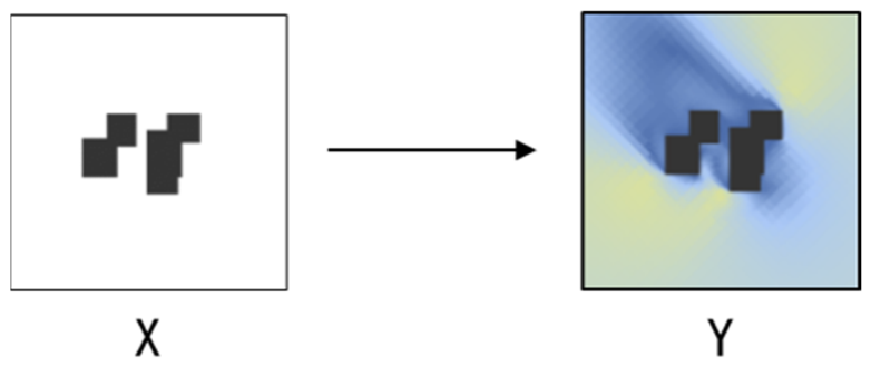
The increasing maturity of deep learning technologies has opened up new avenues for analysis and prediction based directly on the building form itself, rather than on manually designed metrics. This is because deep learning algorithms bypass manually designed morphological metrics and, through end-to-end learning, can directly uncover the complex relationships between morphological patterns and performance that are difficult to identify using traditional methods. In current research on wind field prediction based on generative models, the results of analyses of a building’s outdoor wind environment are typically approximated using mathematical mappings. The abstracted mathematical model serves as a bridge between architecture and machine learning; by encoding this mathematical model, machine learning models can be established to achieve rapid prediction of a building’s outdoor wind environment. Such research typically involves two datasets: X (building geometry) and Y (CFD flow field). The objective is to capture the conditional mapping between the X and Y data (as shown in Figure 1).

This type of prediction method is typically trained on large-scale datasets to achieve generalization, which entails significant training costs, including data collection, data processing (such as cleaning, annotation, and feature extraction), and computational resource consumption (such as training time and energy consumption of GPUs/TPUs). These costs are particularly pronounced when dealing with large urban areas, as models must account for diverse topography, architectural forms, and climatic conditions, leading to an explosive growth in data requirements and challenges related to generalization.

To address this challenge, this study proposes a design task-oriented prediction method called Site-Specific Training for Design Tasks (SST-DT). The core principle of this approach lies in confining training scope to specific design scenarios rather than pursuing cross-city or large-scale universal models, thereby significantly reducing costs while ensuring highly design-specific predictions.

2.

Development of the Prediction Model Based on the SST-DT Strategy

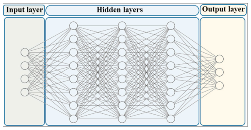
Current research on machine learning-based outdoor wind environment prediction for buildings primarily employs various deep neural networks as predictive models. These models typically utilize multi-layer neural network architectures to facilitate information transfer, with their structures generally comprising input layers, hidden layers, and output layers (as shown in Figure 2).

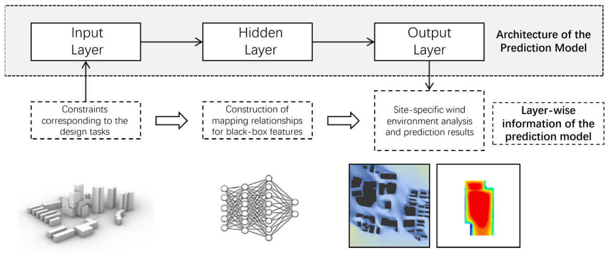
The core principle of SST-DT proposed in this study is “task-oriented local training,” which restricts model training and application to specific sites within the designed tasks to minimize costs. A single SST-DT-based prediction model primarily consists of three components: an input layer for design conditions, an output layer for analysis results, and an implicit layer that establishes spatial morphology encoding inputs and performance simulation result mappings through mathematical computations (as shown in Figure 3).

• Input Layer: Constraint Information

Input parameters refer to data applicable to a model, which are used to describe or characterize the problem the model aims to solve. When building a model, selecting appropriate input parameters significantly impacts its predictive performance and accuracy. The choice of input parameters should also be based on the requirements of the design task.

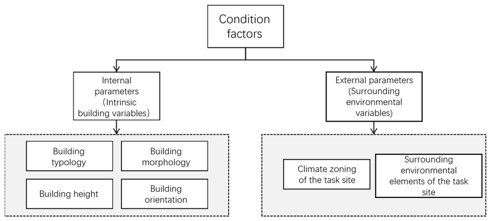
The analysis process of building outdoor wind environments is constrained by numerous conditions, which collectively influence the mapping relationship between performance analysis and architectural spatial morphology. Therefore, the input parameter information comprises two components: conditional elements and control elements (as shown in Figure 4).

Condition factors refer to parameter constraints that influence building performance analysis in design. In this study, the constraint parameters used to predict outdoor wind environments for buildings can generally be categorized into two types: external parameters and internal parameters. External input parameters typically describe environmental variables surrounding the building, including the climate zoning of the project site and its adjacent environmental elements. Internal input parameters, on the other hand, are used to characterize building-specific characteristics such as architectural type, form, height, and orientation.

Control elements refer to regulatory conditions distinct from conditional factors. These elements vary across individuals and projects, exhibiting inherent uncertainty. Given the complexity of control elements and the constraints of this study’s scope, we focus exclusively on key and common rectangular volume combinations in design practice. Such volumes adhere to specific modular principles and can all be represented within a three-dimensional orthogonal grid framework.

• Hidden Layer: Construction of “Black-Box” Mapping Relationships

Performance physics calculations conducted through simulation software can be classified as white-box methods, which allow clear interpretation of computational principles at each simulation stage and enable direct observation of system internal structures. In contrast, machine learning-based computational approaches represent black-box methods that only process spatial morphology-encoded inputs and performance simulation outputs, establishing mathematical mappings between them. For specific shape encoding patterns, this strategy significantly enhances computational efficiency compared to direct performance simulations. Technically, the hidden layers constitute the algorithmic architecture of machine learning models. While this study does not resolve the fundamental opacity of deep learning, the SST-DT strategy partially mitigates interpretability concerns by confining the operating domain to a single site and task: the reduced input space allows designers to build an intuitive understanding through systematic parameter variation, and the pixel-wise output format enables direct visual comparison with CFD results to identify regions of high relative error.

• Output Layer: Performance Simulation Results

Image-based DL models enable transformations such as converting semantic/labels into real images and grayscale images into color images, with their fundamental objective being pixel prediction. This study investigates the relationship between architectural forms and physical properties, aiming to elucidate the correlation between form parameter encoding and building physical performance. By generating new samples and deriving corresponding performance analyses through multi-variable mapping to a single dependent variable, the output of deep learning-driven outdoor wind environment prediction for buildings should represent simulated computational results of outdoor wind conditions, visually represented using color coding methods.

3.1.2. Procedural Framework

The implementation steps of the prediction process based on the SST-DT strategy are designed in a modular and highly operational manner, facilitating its application by architects or engineers in design practice. The framework can be divided into two phases: training and application. The specific workflow during the training phase includes:

• Project definition and site delineation: collecting project requirements, including climate conditions at the task site and surrounding environmental information. Then, generate batch parameterized models related to the design task using a generative tool;
• Dataset: the prediction is defined, followed by CFD simulations and data post-processing to construct a robust dataset;
• Model training: train the deep learning model based on the dataset.

The primary objective during the application phase is to deploy the trained machine learning model to real-world architectural design challenges. Key steps include: (1) Loading design proposals into the trained model, ensuring the data matches the input format and features from the training phase; (2) Using the trained model to predict input data and generate forecast results.

This framework is designed to position architects as the primary practitioners, providing technical support for performance-driven design processes. It facilitates interdisciplinary parameter coordination, integrates performance simulation, and enhances design decision-making support. To address architects’ growing demand for performance-based design optimization technologies during the design process, the framework establishes neural network models tailored to specific site conditions within design tasks. This paradigm shift moves from generic models to task-oriented training for particular sites, with computational resources exclusively allocated to design scenarios. Consequently, it delivers timely, high-quality design feedback to architects.

3.2. Automated Model Construction

3.2.1. Automated Framework

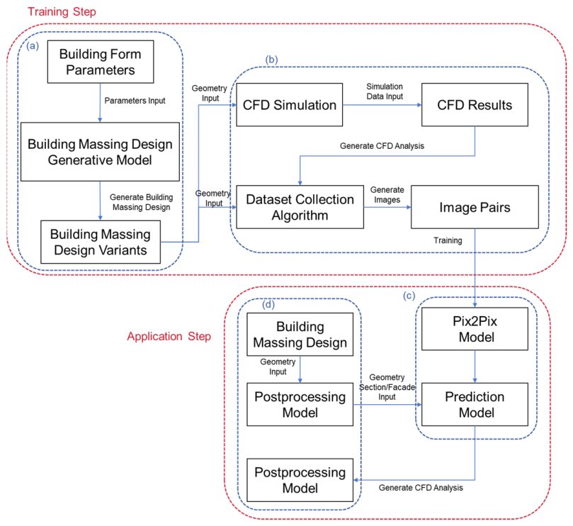
This study proposes a model construction method centered on a workflow integrating automated annotation labeling and sample generation modules. The approach effectively addresses the challenges architects face during machine learning implementation, as outlined in Section 1, specifically the issues of high entry barriers, time-consuming processes, and low efficiency. The overall framework of this method is illustrated in Figure 5.

In summary, this workflow establishes a recursive loop connecting generative tools, performance simulation programs, and deep learning models. The loop automatically completes building volume generation, performance evaluation, dataset construction, and deep learning model training. Essentially, our study proposes an automated framework that enables complex CFD simulations and deep learning model training without requiring specialized technical expertise. The automated model construction process comprises two phases: training and application. The training phase follows a predefined workflow, including generating parametric models with diverse geometries using generative tools (Figure 5a), creating training datasets (comprising CFD simulation tasks (Figure 5b) and data post-processing tasks), and training deep learning models based on these datasets (Figure 5c). The application phase aims to utilize trained machine learning models to solve real-world architectural design challenges (Figure 5d).

3.2.2. Selection of the Prediction Model

In this study, the Pix2Pix model was selected as the prediction framework. Pix2Pix enables the use of architectural geometry models as input data for wind environment prediction, aligning with CFD results to develop a novel method for accelerating building wind field analysis. The Pix2Pix architecture consists of a generator (implemented using the U-Net framework) and a discriminator (based on PatchGAN architecture). In the generator module, the encoder employs layer-by-layer downsampling convolutional operations to reduce the size of input architectural images (e.g., CAD models or point cloud renderings), capturing features across different scales (including building contours and spatial configurations). The decoder then performs progressive upsampling inverse convolution operations to restore original scales while utilizing skip connections to retain fine details such as window openings and protruding structures. The discriminator adopts PatchGAN’s design philosophy, dividing input images into N × N patches and evaluating their realism individually. This process focuses on high-frequency wind field characteristics (e.g., wind speed gradients and vortex peaks) rather than overall wind environments. Additionally, the recognizer utilizes stacked convolutional layers to extract multi-level features from micro-turbulence patterns into macro-scale flow fields (e.g., building wake zones).

Pix2Pix controls the authenticity of generated results by jointly optimizing the adversarial loss and L1 loss, where the mathematical expression of the adversarial loss is shown in Formula (1): The adversarial loss formulation follows the conditional GAN objective of Isola et al. [36], which also introduces the PatchGAN discriminator architecture adopted in this study.

$${\mathcal{L}}_{\mathrm{G}\mathrm{A}\mathrm{N}}(\mathrm{G},\mathrm{D})={\mathbb{E}}_{\mathrm{x},\mathrm{y}}\left[\log \mathrm{D}\left(\mathrm{x},\mathrm{y}\right)\right]+{\mathbb{E}}_{\mathrm{x}}\left[\log \left(1-\mathrm{D}(\mathrm{x},\mathrm{G}(\mathrm{x}\right)\left)\right)\right]$$

(1)

x is the input architectural image and y is the ground-truth wind map. The adversarial loss encourages outputs that share the CFD data’s statistics; an additional L1 loss enforces pixelwise alignment: The L1 regularization term is likewise adopted from the original Pix2Pix framework [36].

$${\mathcal{L}}_{\mathrm{L}1}\left(\mathrm{G}\right)={\mathbb{E}}_{\mathrm{x},\mathrm{y}}\left[{‖\mathrm{y}-\mathrm{G}\left(\mathrm{x}\right)‖}_1\right]$$

(2)

In conclusion, Pix2Pix demonstrates significant advantages in two fields: multi-scale feature balancing and high efficiency in data processing and training. For the first field, this architecture enables the generator to better understand the complex relationship between architectural geometric models and wind speed variations, thereby more accurately predicting detailed wind speed field information. The discriminator utilizes a PatchGAN structure to perform pixel-level authenticity evaluation on generated wind speed field images. This local discrimination mechanism helps the generator better learn detailed wind speed field characteristics, enhancing the accuracy and realism of prediction results. For the other field, Pix2Pix is capable of processing complex architectural geometric models and environmental data; the encoder reduces three-dimensional architectural models to two dimensions, then overlays them with environmental performance datasets and encodes the images, enabling the training set to be utilized more effectively in model training. Compared to some physics-based algorithms, the training process for Pix2Pix is relatively simple and efficient. It does not require complex meshing or extensive computations; instead, it utilizes a large volume of training data to allow the model to automatically learn the mapping relationship between input and output images, thereby rapidly generating wind speed field predictions.

3.3. Automated Data Acquisition

3.3.1. Methodology for Dataset Generation

Currently, when architects use CFD analysis methods based on machine learning, they are required to carry out a significant amount of feature engineering work in advance. Feature engineering is a substantial and time-consuming task, involving various aspects of machine learning knowledge, such as feature selection and data pre-processing. To automate this process, a straightforward strategy would be to eliminate the need for architects to perform parametric modeling and set up simulation workflows when conducting CFD simulations. Furthermore, in addition to reducing the architect’s workload in parametric modelling and workflow setup, the tagging of features and sample generation for CFD analysis should also be accomplished with minimal intervention from the architect. Consequently, this study adapts the feature engineering process by incorporating the aforementioned improvements in both areas.

1.

Optimization Strategy for CFD Simulation Workflows

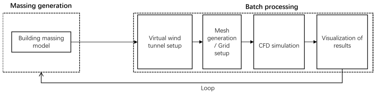
CFD supports the evaluation of airflow, thermal transport, wind conditions, comfort, and energy use in buildings. The workflow includes: (i) domain definition, (ii) mesh generation, (iii) boundary/physics setup, and (iv) post-processing. Geometry is converted into a mesh and, after simulation, outcomes are visualized (Figure 6).

Although simulation tools are capable of handling all four stages, the standard practice is to create and edit 3D models in software such as Rhinoceros 3D or Revit, and then convert them into a suitable format for import into CFD simulation software (Buterfly, v1.10). Following the solution in the simulation software, the results often need to be exported to another program, such as ANSYS CFD-Post or ParaView, to visualize the outcomes. Although the process of these stages appears straightforward, it presents numerous challenges as it is prone to errors, whether arising from model export between different platforms or from incorrect programming or inappropriate solver parameter settings. Whilst CFD plugins integrated into design platforms can resolve cross-platform transfer issues, these plug-ins, with their limited functionality, have inherent limitations in practical application. Firstly, although plugins can simplify the CFD simulation workflow, specialist CFD knowledge remains essential in practice. Furthermore, when using plugins with immature graphical user interfaces, users lack clear guidance regarding workflow and simulation operations.

In summary, the entire CFD workflow is time-consuming and requires significant manual intervention; however, there is currently a lack of software integrated into design platforms that enables automated calculations, and tools combining computational capabilities with programming languages are virtually non-existent. To address the difficulties in using CFD tools arising from the gap between the engineering nature of CFD and the creative orientation of architectural design, this study involves the secondary development of CFD simulation tools using the Python language. This aims to automate CFD simulations whilst providing users with pre-set templates and a simplified interface, thereby lowering the barrier to entry for users with limited engineering backgrounds. The specific technical approach is as follows: first, a generation module batch-generates architectural volume models to construct a library of parametric models under the current parameters. Once the volume generation is complete, initial simulation workflow settings are configured via the user interface, including a set of simulation templates requiring only a minimal number of input parameters. Finally, the process proceeds to the batch processing module for the various stages of unified simulation and computation. This workflow enables the independent simulation of all imported models without the need for manual selection or intervention, and automatically initiates the next simulation upon completion of the first, thereby achieving full automation of simulation and computation (the workflow is illustrated in Figure 7).

2.

Optimization of the Sample Generation Workflow

With the advancement of AI, people hope that AI will free them from mechanical and tedious tasks. In machine learning, feature engineering accounts for 80% of the work, whilst model training accounts for only 20%. The traditional approach to feature engineering involves using domain knowledge to construct features one by one; this is a lengthy, time-consuming, and error-prone process known as manual feature engineering. Manual feature engineering is inefficient and lacks portability; features created manually are often only suitable for specific problems.

Therefore, if feature engineering is also automated, the efficiency of machine learning can be significantly improved. In the field of ML, automated feature engineering refers to the automatic extraction of useful and meaningful features from a set of relevant data tables, utilizing a framework that can be applied to any problem, with the ultimate aim of improving standard workflows. This includes automated feature extraction, automated feature pre-processing and automated feature compression. In this study, however, as specific feature content and formats are already available, automated feature engineering has been simplified to the task of automated sample generation.

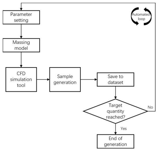
Figure 8 illustrates the workflow for automated data set acquisition. In brief, this workflow interconnects the generative tool and performance simulation program through a recursive loop. The loop automatically generates architectural volumes and constructs the data set. The process involves using the generator tool to produce parametric models in various morphologies, followed by building the training dataset through CFD simulation and data post-processing tasks.

3.3.2. Construction of the Horizontal Wind Field Dataset

This study leveraged ParaView for automated data processing. The procedure involves steps:

1.

Extraction and Visualization:

Initially, the architectural layout and its corresponding horizontal wind flow slice at a pedestrian height of 1.5 m above the ground were extracted. To characterize the wind speed variations at this height, the Plasma colormap from the matplotlib library was utilized to map wind velocity values within a range of 0–12 m/s onto the RGB color space. Converting wind speeds into visualized RGB images enables a clear representation of velocity gradients and spatial fluctuations across the target domain.

2.

Image Acquisition and Annotation:

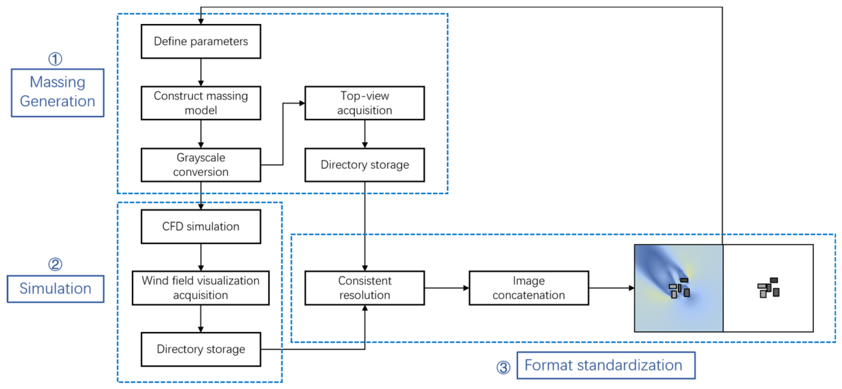
We annotated target regions with closed polygons (multiple vertices) and captured images automatically using PIL’s ImageGrab, which crops a top-down square via four bounding points, then returns pixel data on Windows. Captured massing snapshots and subsequent CFD wind-field outputs are saved to predefined directories (Figure 9).

3.

Spatial Resolution and Dataset Partitioning:

To maintain uniform input dimensions for the deep learning model, the extracted images were standardized to a resolution of 256 × 256 pixels, with each pixel representing a spatial extent of 2.5 m.

Since the same building shape looks similar when rotated or resized, random splits could leak information between training and test datasets. So we grouped every version of a single geometry into the same split. The method in each subset contains different geometries, keeping evaluation fair while preserving dataset variety.

In supervised learning, the original training set is typically divided proportionally into a training set and a validation set. The training set is used to build the model, while the validation set evaluates its performance on unseen data, thereby estimating the model’s generalization ability. In this study, a simple random split method was employed for dataset partitioning, with a split ratio of 8:2 (training set:validation set).

3.3.3. Construction of the Elevation Wind Pressure Dataset

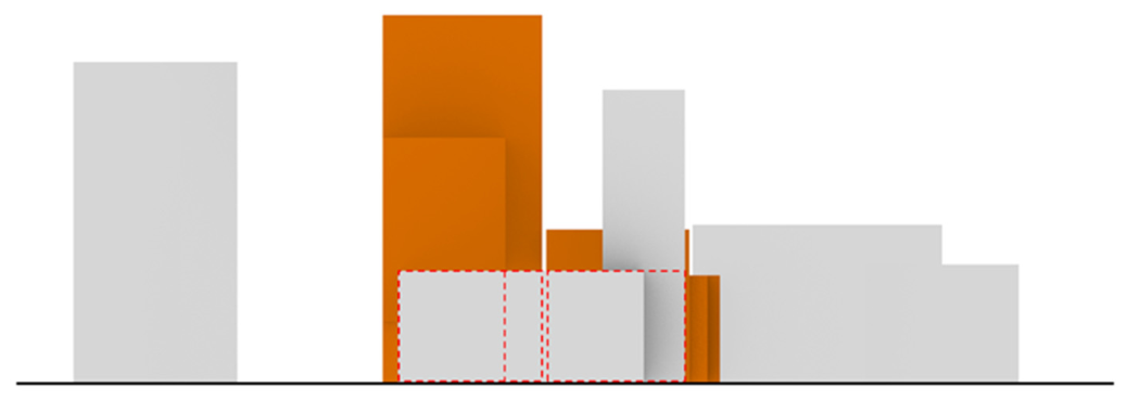
For one-building datasets, we feed massing images in and predict wind-speed or pressure maps. CFD tools let you rotate the scene in 3D to see every surface, but our image-based models need a single, fixed 2D view. That causes visual occlusion: nearer buildings can block the pressure or vector patterns on buildings behind them (highlighted by the red dashed areas in Figure 10), so some local high- or low-pressure zones become hidden. In short, geometric shielding, complicated flow behavior, and the loss of depth in 2D images are the root causes.

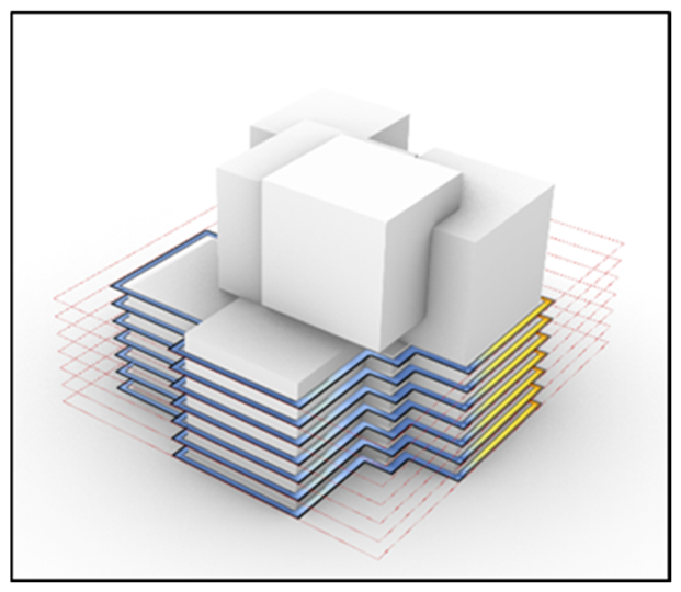
To see what’s hidden behind foreground buildings, the 3D CFD results are sliced at set heights and save those cross-sectional pressure maps. These “static slices” cut through geometric barriers and uncover the flow and pressure patterns that a single camera view would miss. The idea borrows from 3D reconstruction in computer vision.

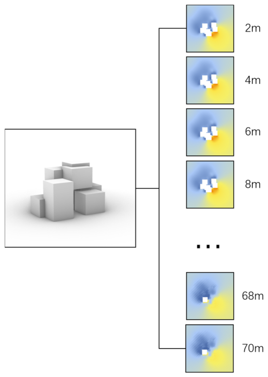
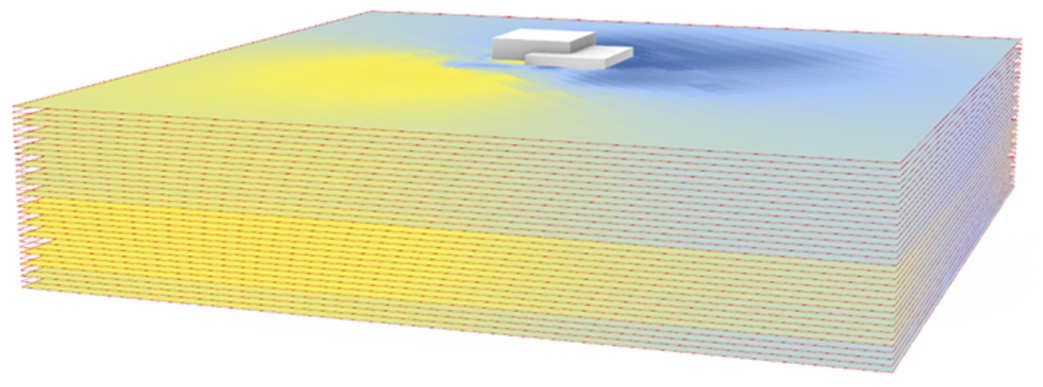
In this context, static slicing refers to extracting wind pressure data on fixed Cartesian planes. While horizontal slices are captured on the XY plane, architectural elevations are typically vertical (e.g., XZ or YZ planes, as shown in Figure 11). The specific implementation steps are as follows:

1.

Data Collection: Raw CFD simulation data is standardized to cover the full height range of the target elevation.

• XY Plane Data Acquisition: Wind pressure data is exported along the Z-axis at fixed 2 m intervals. And a 50 m building yields 25 slices. Each slice consists of 2D grid data containing pressure values and spatial coordinates.
• Data Standardization: Slices are normalized into a 256 × 256 grid format. Noise (e.g., zero-value regions inside the building footprint) is removed to facilitate downstream processing.

2.

Coordinate Alignment and Elevation Mapping: Horizontal slice data is projected onto vertical planes to achieve 3D-to-2D reconstruction.

• Defining Target Elevations: Suppose we need to reconstruct the west façade of a building (where X is a fixed value). We extract all points in the XY plane where the X-coordinate is close to this value, forming a vertical data band distributed along the Z-axis (Figure 12). We then iterate through each slice, selecting column data where the X-coordinate falls within the threshold range.
• Creating the Elevation Grid: As shown in Figure 13, a two-dimensional grid matching the resolution of the original data is established in the XZ plane, with each node corresponding to specific coordinates; NumPy arrays are used to stack the slice data.

3.

Edge Detection and Indexing: Locates geometric contours and uses labeling to interactively hide obstructing objects, facilitating the observation of obscured areas.

• Edge Detection: Edge detection in images is a fundamental step in image processing and constitutes a key area of research within the field. Its primary principle lies in identifying pixels within digital images where there are marked changes in color or brightness; these significant changes in pixel characteristics often indicate important alterations in the properties of that part of the image, including discontinuities in depth, direction, and brightness. When performing edge detection, edge detection algorithms first identify a rough outline of the image by detecting certain pixels. These pixels are then connected using specific linking rules. Finally, previously unidentified boundary points are detected and connected, whilst false pixels and boundary points are removed to form a complete edge. There are currently many commonly used edge detection models: first-order operators include the Roberts operator, the Prewitt operator, the Sobel operator and the Canny operator; second-order operators include the Laplacian operator, amongst others. Image edge detection is based on image gradients, and obtaining these gradients involves applying various operators to the image through convolution operations. In this study, the Canny operator is employed to precisely locate the contours of geometric shapes within planar slices, with Canny thresholds set at 50 (low threshold) and 150 (high threshold) to capture building boundaries. The Canny edge detector [41] is selected for its established performance in precisely locating geometric contours at sub-pixel resolution.
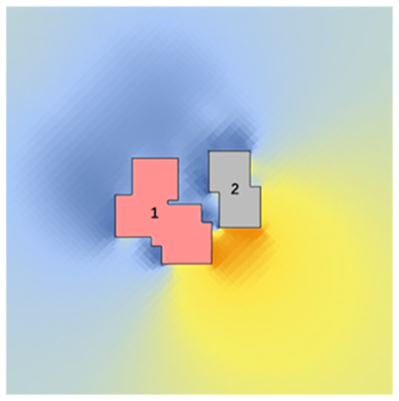
• Indexing: In order to interactively adjust the visibility of geometric shapes within a slice in a two-dimensional image, the author assigns a numerical identifier to each closed shape in the image. Each closed shape is assigned a numerical identifier (starting from 1). The contour hierarchy (returned by OpenCV’s ‘findContours’) is used to distinguish between inner and outer contours, which are then sorted by area or position. Numbering allows for the selective hiding of foreground structures in the reconstructed image. This enables the concealment of obstructions as required, facilitating the observation of wind pressure distributions in the obscured areas (as shown in Figure 14, where the foreground structure numbered 1 can be hidden to reveal the wind pressure on the background structure 2).

4.

Morphological Dilation-Based Color Mapping: This step ensures accurate color filling and spatial continuity of the wind pressure data.

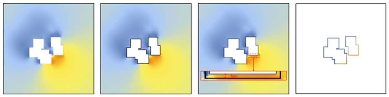
• Morphological Dilation: A 3 × 3 structural element is used to perform a 2-pixel dilation on the original contours. Dilation expands foreground regions, ensuring that the pressure colors cover any gaps or noise near the boundaries (Figure 15).
• Sampling and Filling: Colors are sampled from non-contour regions adjacent to the boundaries and mapped to RGB space based on wind pressure values. When an occluding building is “hidden,” its corresponding mask is set to transparent.

5.

Vertical Interpolation and Anti-Aliasing: After obtaining sufficient horizontal (XY) slices, the data must be converted into a continuous vertical elevation map.

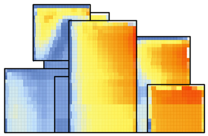
• Data Interpolation: As shown in Figure 16, the sampled contours are overlaid along the Y direction, and the Y direction (i.e., different XY slices) is differentiated for each XZ grid point. Since the spacing between adjacent slices is small and the data is smoothed in this experiment, linear interpolation is used to calculate intermediate values. The differentiation formula is presented in Equation (3). This linear interpolation–differentiation scheme was derived by the authors for the static slicing reconstruction procedure described in this study.

$$C_p(z)=C_p(z_i)+{\displaystyle \frac{z-z_i}{z_{i+1-z_i}}}\left(C_p\left(z_{i+1}\right)-C_p\left(z_i\right)\right)$$

(3)

Here, ${\mathcal{C}}_{\mathcal{P}}$ represents the wind pressure slice, ${\mathcal{Z}}_{\mathcal{i}}$ and ${\mathcal{Z}}_{\mathcal{i}+1}$ represents the height of the adjacent slice. The post-difference effect is shown in Figure 17.

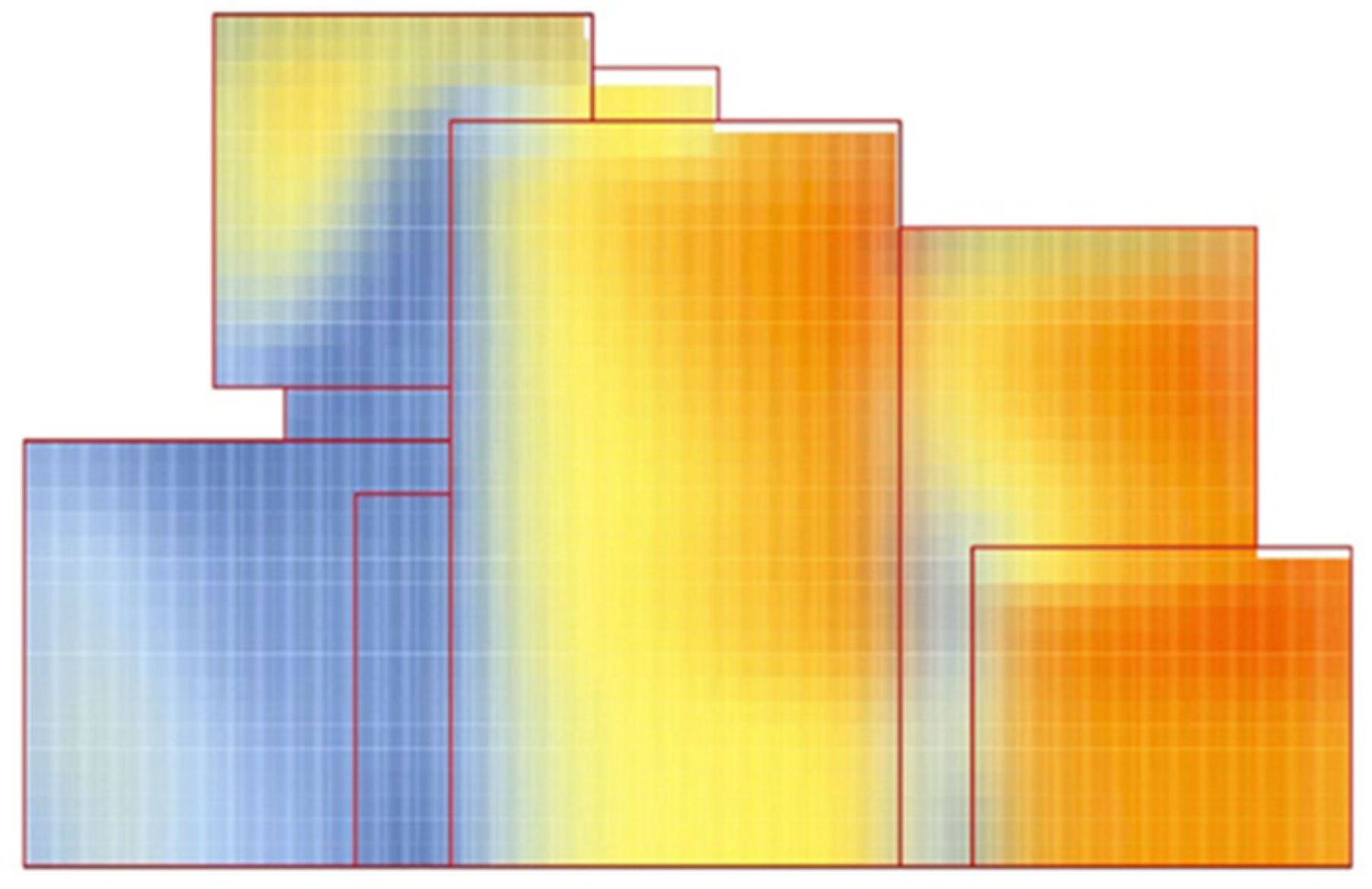
• Post-processing via Anti-Aliasing: As can be seen from the figure above, the elevation view reconstructed using the difference method consists of a grid of square pixels. When the number of slices is insufficient, the reconstructed elevation view will exhibit noticeably jagged edges due to discrete sampling. In theory, reducing the slice spacing to increase the number of slices can increase the density of the pixel grid, thereby making the color transitions in the reconstructed elevation view smoother. However, an excessively high number of slices would significantly increase computational costs, severely impacting design efficiency. Therefore, under conditions of insufficient slice sampling, post-processing of the image is required, namely anti-aliasing. Common anti-aliasing methods include Super Sampling Anti-Aliasing (SSAA), Multi-Sampling Anti-Aliasing (MSAA), Fast Approximate Anti-Aliasing (FXAA), Temporal Anti-Aliasing (TAA), and Coverage Sampling Anti-Aliasing (CSAA). Among these, Fast Approximate Anti-Aliasing (FXAA) can rapidly eliminate visual discontinuities by intelligently blurring jagged edges in the image without relying on high sampling rates. As this technique strikes a good balance between visual quality and computational resources, this study adopts this method for the post-processing of elevation views. The anti-aliased elevation view is shown in Figure 18 below. As can be seen from the figure, depending on the direction of the edge (horizontal or vertical), the color along the edge’s direction is blended with that of adjacent pixels, resulting in a smoother color transition where jagged edges would otherwise appear. This significantly improves the aliasing issues caused by insufficient sampling. FXAA is implemented following the algorithm described in Lottes [42].

4. Experimental Design and Results Analysis

Based on the working framework proposed in this paper, architects can rapidly develop a customized system for wind field analysis of a specific site, and apply this system to various architectural design tasks. The following sections validate the effectiveness of the proposed framework using design tasks from four different cities—Shanghai, Nanjing, Beijing and Guangzhou—and demonstrate its application in architectural design performance-related tasks. The design subject is a high-rise tower office building in each of these cities, with the prediction targets being wind speed at pedestrian height (1.5 meters) and wind pressure on the building façade. The specific design parameters for the target building are as follows: 25 stories, 9 bays in width, 8 bays in depth, a column spacing of 8.4 meters, and a target floor area of 55,000 square meters (

Table 1. Location of the practice project site, surrounding environment, and local wind rose diagram.

Cities	Location of the Practice Project Site and Surrounding Environment	Wind Rose Diagram
Shanghai
Nanjing
Beijing
Guangzhou

). It should be noted that in this case study, we primarily conduct quantitative analysis using two metrics: simulation efficiency and accuracy.

4.1. Experiment 1: Prediction of Outdoor Pedestrian-Level Wind Environment

4.1.1. Massing Model Parameters

The architectural volume model is generated using the additive form generation algorithm from the Rhino-Grasshopper plugin EvoMass. EvoMass is a design tool that adapts to various architectural volume design configurations, enabling architects to conduct rapid, optimization-driven design exploration. In EvoMass’s design generation module, specific design objects (such as high-rise towers, slab buildings, or atrium structures) are not treated as abstract modeling entities. Instead, two fundamental architectural volume manipulation principles—“volume addition” (additive) and “volume subtraction” (subtractive)—serve as the basis for parametric modeling. This generation model can be regarded as a “meta-model” for generating architectural volumes: under varying parameter controls, it derives sub-models tailored to different building types, endowing EvoMass with high generalization capability and reusability at the design generation level.

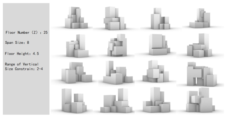
Regarding the volumetric model parameters in this chapter’s experiments, the design object is defined as a high-rise tower-style office building characterized by a limited number of large-scale elements. Four sets totaling 1000 building volumetric models were generated, with vertical elements controlled at 3–5 units, horizontal elements at 5–6 units, and Z-direction elements at 25 units. The floor height was set at 4.5 m with column spacing of 8.4 m. Figure 19 demonstrates the specific parameter configurations and selected volumetric models produced.

This study employed Python scripts in Paraview for data processing to ensure consistency and usability. First, architectural layout information and corresponding pedestrian horizontal airflow slices at 1.5 m above ground level were extracted. To represent wind speed variations at pedestrian height, the matplotlib Plasma legend was utilized to map wind speeds within the 0–12 m/s range into the RGB color space, converting wind data into visualized RGB images. This method enables clear visualization of wind speed fluctuations across different areas.

4.1.2. CFD Simulation Parameters

Shanghai, Nanjing, Beijing, and Guangzhou are located in the eastern coastal region of China, the inland area of the lower Yangtze River, the North China Plain, and the Pearl River Delta region of South China, respectively, exhibiting distinct climatic and urban morphological differences. Using these four cities as case studies covers various architectural climate zones and wind environment characteristics, all of which have substantial demands for high-rise office building design and are suitable for pedestrian wind environment and facade wind pressure analysis. Together, these four cities form a representative test dataset to evaluate whether the Auto_Wind system can effectively predict wind environments for high-rise buildings under diverse urban wind climates and complex urban morphological conditions.

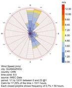
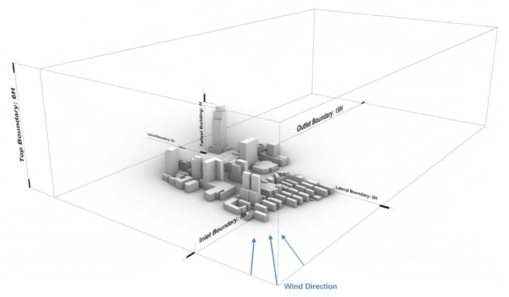
In this experiment, the computational range was defined based on the overall building dimensions (Figure 20). The vertical height calculation range was set at 5H (H = maximum building height), while the lateral boundary and inlet boundary calculation ranges were both 5H, and the outlet boundary calculation range was 15H. Subsequently, wind speed and wind direction were determined using meteorological data. Boundary conditions were derived from local meteorological data for four representative Chinese cities:

• Shanghai: Located in a subtropical monsoon zone (30°40′–31°53′ N, 120°51′–122°12′ E). Prevailing summer winds: SE at 3.4 m/s; winter: NW at 3.5 m/s;
• Nanjing: Subtropical monsoon zone (31°14′–32°37′ N,118°22′–119°14′ E). Prevailing summer winds: SE at 3.5 m/s; winter: NE at 2.8 m/s;
• Beijing: Temperate monsoon zone (39°54′–41°6′ N,115°7′–117°4′ E). Prevailing summer winds: SE at 2.2 m/s; winter: NW at 2.0 m/s;
• Guangzhou: Subtropical monsoon zone (22°26′–23°56′ N,112°57′–114°3′ E). Prevailing summer winds: SE at 1.9 m/s; winter: NW at 2.1 m/s.

These experiments with summer monsoon winds from various cities as input parameters for wind speed and direction. The grid configuration features a 200 × 200 × 50 cell size with refinement settings of (3, 3) and a minimum cell dimension of 1 m. The solver employs the high-efficiency RNG k-ε model for turbulence kinetic energy calculation, with 150 iteration cycles configured. Landscape roughness parameters reflect dense urban environments at a reference height of 10 m above ground, using an input reference wind speed of 10 m/s to simulate typical gusts caused by urban dynamic topography. All other parameters remain consistent with default settings.

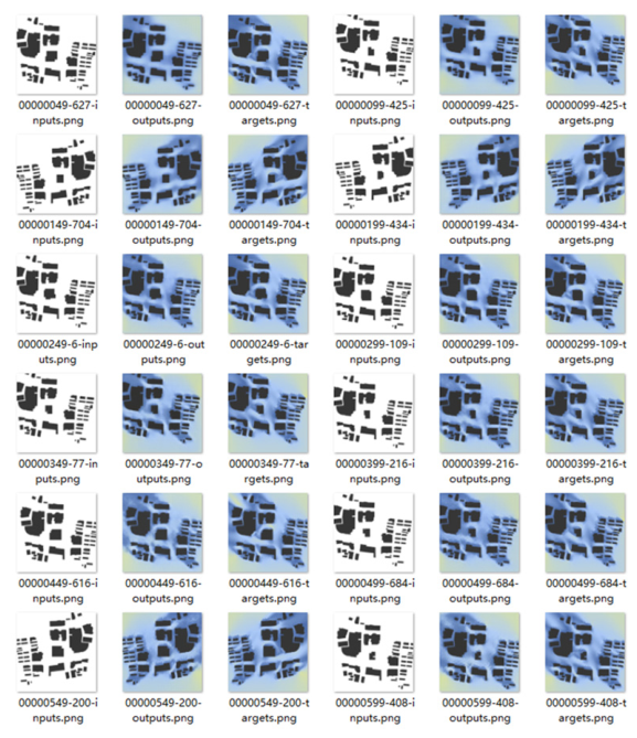
For training, the learning rate was set to 0.0005, with the Adam optimizer used to train both the generator and discriminator. The momentum parameter was configured at 0.65, and both input and output resolutions were maintained at 256 × 256 pixels. Batch size was set to 1, and the generator network adopted a 9-block UNET architecture. To suppress model oscillations, the pooling parameter was set to 50. The dataset was trained over 800 epochs with 50 epochs as intervals, and training weights were saved to track progress. Training was conducted on a computer equipped with a GeForce RTX 3070 graphics card, with each epoch averaging 25 s in duration (partial training results are shown in Figure 21). The generator and discriminator were initialized using a normal distribution with mean 0 and standard deviation 0.5. The lambda parameter for L1 loss was set to 100, and the model converged after approximately 60,000 iterations. The Pix2Pix model was implemented using Python 3.7 and the open-source machine learning platform TensorFlow on a Windows 10 system equipped with a 3.60 GHz i7 CPU.

During training, a fixed batch size was maintained throughout the entire process. For convergence evaluation, the model’s performance during training and validation phases was monitored by analyzing the loss curve to determine whether convergence had occurred and to identify potential overfitting or underfitting. A gradual decrease in training loss accompanied by an increase in validation loss may suggest overfitting; significant loss fluctuations may indicate an improperly tuned learning rate; and cessation of loss decline may signify model convergence or entrapment in a local minimum. For Pix2Pix, since it combines adversarial loss and L1 loss, the losses of both the generator and discriminator must be monitored simultaneously. A decline in the generator’s L1 loss, accompanied by fluctuations in the adversarial loss, may be normal as the discriminator improves. If the discriminator’s loss approaches zero, it may indicate mode collapse. The training process requires balancing these two losses to ensure the adversarial loss does not become excessively low while maintaining a steady decline in the L1 loss. Finally, this study employs an early stopping strategy to prevent overfitting: training is terminated when the model’s performance on the validation set shows no further improvement for a sustained period, rather than continuing until the maximum number of epochs.

4.2. Experiment 2: Prediction of High-Rise Building Facade Wind Pressure

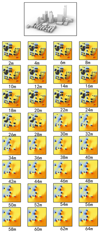
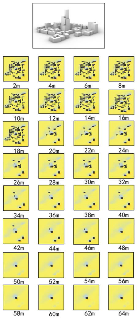
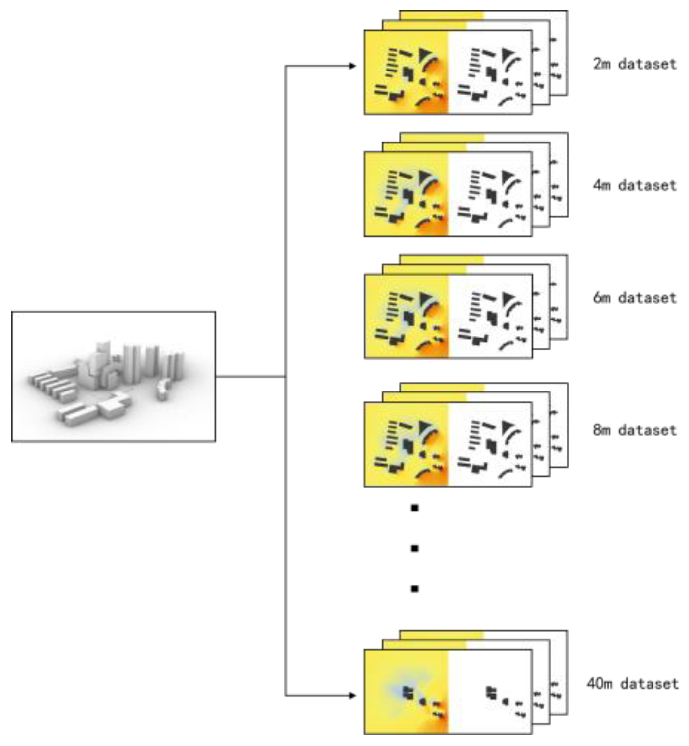
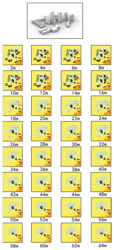
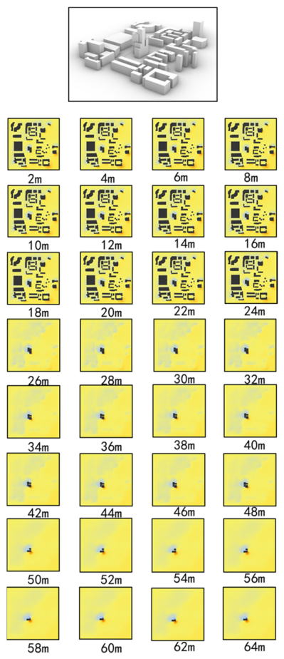
The experimental model in this section continues to utilize the volumetric model generated in Section 4.1 In this experimental section, wind pressure data were calculated across multiple XY planes at fixed intervals of 2 m per floor along the building height (Z-axis), resulting in cross-sectional wind pressure datasets at various heights that comprehensively cover the target facade’s vertical range (as shown in Figure 22).

In this test, a block model not present in the training set was generated for each of the four urban plots to serve as the validation model (Figure 23). After generation, the model was sliced at fixed 2 m intervals using the ExportPlanSection operator and exported as a 256 × 256 prediction image (Figure 24).

After completing dataset construction, the Pix2Pix model training commenced. All training parameters in this section remained consistent with those specified in Section 4.1.

4.3. Results and Discussion

4.3.1. Results Analysis of Experiment 1

1.

Efficiency Comparison

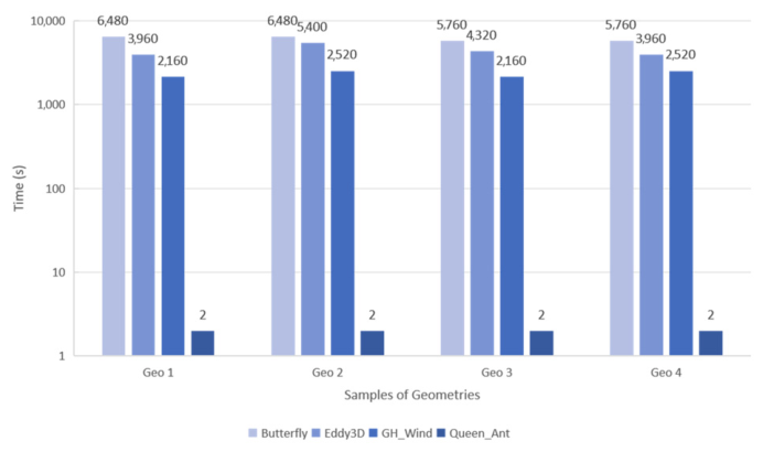
Firstly, in order to assess the computational efficiency of CFD, the time required for each calculation was recorded and compared. It is well known that there are always discrepancies between the results of CFD numerical simulations and those of physical wind tunnel tests. The ML-based CFD prediction method proposed in this study to confirm the extent to which this method can reproduce the established experimental procedures and results. The specific parameters for Butterfly, GH_Wind and Eddy3D are shown in

Table 2. The specific parameters of three common analog tools in the experiment.

	Butterfly				GH_Wind				Eddy3D
Test	Geo_1	Geo_2	Geo_3	Geo_4	Geo_1	Geo_2	Geo_3	Geo_4	Geo_1	Geo_2	Geo_3	Geo_4
CFD modeling methods	PISO	PISO	PISO	PISO	FFD	FFD	FFD	FFD	PISO	PISO	PISO	PISO
Turbulence models	RNGk Epsilon	RNGk Epsilon	RNGk Epsilon	RNGk Epsilon	N/A	N/A	N/A	N/A	RNGk Epsilon	RNGk Epsilon	RNGk Epsilon	RNGk Epsilon
Cell size (m)	0.987552	0.987552	0.987552	0.987552	5	5	5	5	3	3	3	3
No. of cells	563,234	567,854	523,341	526,635	331,477	352,694	341,346	365,751	333,701	357,719	346,562	337,906
Iterations	500	500	500	500	600	600	600	600	800	800	800	800
Time	1.8 h	1.8 h	1.6 h	1.6 h	0.6 h	0.7 h	0.6 h	0.7 h	1.1 h	1.5 h	1.2 h	1.1 h

, where Geo_1 is a volumetric model generated from the Shanghai terrain, Geo_2 from the Nanjing terrain, Geo_3 from the Beijing terrain, and Geo_4 from the Guangzhou terrain. As can be seen from the table, for extensive urban areas, tools such as Butterfly and Eddy3D, which employ traditional CFD analysis methods, typically require over an hour to complete the calculations for each site. In contrast, the GH_Wind tool utilizes the FFD method to solve the Navier–Stokes equations, thereby significantly improving simulation efficiency. However, the simulation time still exceeds 40 min(Since the CFD for the GH_Wind tool in Table 2 employs the FFD method rather than the traditional Navier-Stokes equations, it does not incorporate turbulence models.).

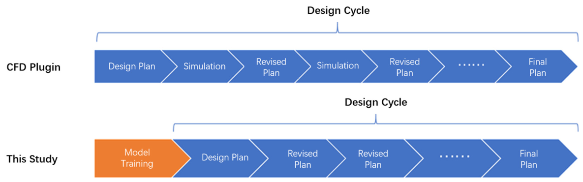
For architects, requiring over 40 min of new simulations after each design modification would significantly prolong the design cycle and frequently disrupt their creative flow. The framework proposed in this study can generate results for large-scale areas within fractions of a second (or seconds, depending on the analysis region’s size). This demonstrates that, compared to other plugins, our approach enables real-time feedback simulation results (Figure 25). Although the predictive model still requires time investment, our framework automatically completes the training process without human intervention. Architects can begin training models before the design cycle starts, thereby dramatically shortening the design cycle (Figure 26).

2.

Accuracy Comparison

To evaluate the predictive performance and generalization capability of the proposed model, 50 novel massing models—none of which were included in the training set—were generated for each of the four target cities (Shanghai, Nanjing, Beijing, and Guangzhou). The ML-predicted results were compared against the real simulations from Butterfly using pixel-wise difference analysis and the Structural Similarity Index Measure (SSIM).

Table 3. Analysis of the prediction results of the test model in Shanghai.

Ground Truth	Prediction	Relative Error	SSIM
			0.8659
			0.9155
			0.9227

,

Table 4. Analysis of the prediction results of the test model in Nanjing.

Ground Truth	Prediction	Relative Error	SSIM
			0.8731
			0.8822
			0.9211

,

Table 5. Analysis of the prediction results of the test model in Beijing.

Ground Truth	Prediction	Relative Error	SSIM
			0.8932
			0.8874
			0.8856

and

Table 6. Analysis of the prediction results of the test model in Guangzhou.

Ground Truth	Prediction	Relative Error	SSIM
			0.8666
			0.9245
			0.9124

summarize the evaluation cases. As indicated in these tables, the SSIM values for the validation models range from 0.84 to 0.92, demonstrating high structural fidelity. Relative error maps further reveal that significant discrepancies are confined to localized regions, ensuring the overall reliability of the predictions.

Specifically, the model demonstrates high accuracy in predicting wind speed distributions within the leeward wake regions. Conversely, larger relative errors are primarily observed in the windward high-velocity zones. This phenomenon can be attributed to the inherent characteristics of the dataset: while wind flow patterns in the leeward wake regions exhibit high consistency across various training samples, the high-velocity zones on the windward side are extremely sensitive to specific building morphologies. The localized errors suggest that the current training sample density may be insufficient to fully capture the complex interactions between diverse building shapes and high-intensity windward flows.

Table 7. The performance metrics of the model’s predictions on Experiment 1.

Dataset	Metric	Statistic	Pix2Pix
Experiment 1	MAE	Average	0.062
		Range	0.041–0.065
	RMSE	Average	0.083
		Range	0.076–0.088
	SSIM	Average	0.973
		Range	0.965–0.988

compares the MAE, RMSE, and SSIM for Pix2Pix’s predictions on the Experiment 1 dataset. The metrics represent the average prediction scores of the trained model on the validation set, with each dataset’s validation set containing 100 images. For MAE and RMSE, values closer to 0 indicate lower prediction errors, while for SSIM, values closer to 1 signify greater structural similarity. The results show that Pix2Pix achieves consistently low MAE (average 0.062) and RMSE (average 0.083), demonstrating effective variance explanation and strong fitting performance. SSIM values approach 1 (average 0.973), indicating high structural similarity between predicted and simulated images.

4.3.2. Results Analysis of Experiment 2

Constrained by the inherent characteristics of 2D imagery, “3D visualization occlusion” represents a significant intrinsic limitation for image-based neural networks. While traditional mitigation strategies—such as transparency adjustments or exploded views—can alleviate this issue, they are often either unintuitive (in the case of isolated cross-sections) or compromise the structural integrity of the model (in the case of fragmented views).

The primary merit of the static slicing technique lies in its ability to directly access the “raw data layer” of the building facade, thereby completely bypassing the complexities and artifacts of the 3D rendering stage. Unlike conventional visualization-based approaches, static slicing addresses the occlusion problem through data-layer reconstruction rather than mere graphical manipulation (as summarized in

Table 8. Comparison of traditional method and static slicing technique.

Comparison Dimension	Static Slicing Technique	Traditional Occlusion Removal Solution
Data Integrity	Directly obtains complete façade data meshes with no occlusion	Relies on viewing angle/transparency; data display is incomplete
Preservation of Spatial Relationships	Preserves the true relative positions of buildings through coordinate mapping	Uses separated views, disrupting true spatial relationships and failing to reflect wind field interference effects between buildings
Batch Processing Capability	After training is completed, all building façades can be processed automatically	Requires manual building-by-building operation

).

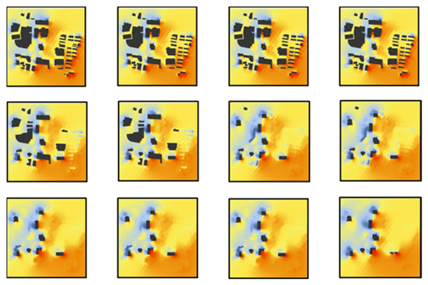
In Experiment 2, specialized predictive models were developed for each horizontal cross-section through targeted training. By performing sequential layer-wise predictions, the wind pressure distribution at every height interval was successfully obtained. Figure 27, Figure 28, Figure 29 and Figure 30 illustrate the predicted wind pressure maps for a novel building massing model across various cross-sectional planes within the urban contexts of Shanghai, Nanjing, Beijing, and Guangzhou.

Table 9. Effect of generating facade wind pressure for test model.

Test Model 1 (Shanghai)	Test Model 2 (Nanjing)	Test Model 3 (Beijing)	Test Model 4 (Guangzhou)

compares horizontal cross-section pressure data with the reconstructed vertical façade pressure maps for the four test models. The reconstructed façades closely match the cross-section predictions and present the results in a form familiar to architects—making them readily usable for practical wind-resistant design decisions in high-rise projects.

Table 10. The performance metrics of the model’s predictions on Experiment 2.

Dataset	Metric	Statistic	Pix2Pix
Experiment 2	MAE	Average	0.039
		Range	0.035–0.042
	RMSE	Average	0.059
		Range	0.048–0.061
	SSIM	Average	0.987
		Range	0.842–0.993

presents the MAE, RMSE, and SSIM for Pix2Pix’s predictions on the Experiment 2 dataset, using the 2 m height dataset from the Nanjing plot as a representative case. For MAE and RMSE, Pix2Pix’s average values fall within a low range (MAE 0.039, RMSE 0.059), indicating good model fit. SSIM averages 0.987, suggesting high structural similarity between predicted and simulated images.

In summary, Experiment 2 demonstrates that the static slicing technique effectively mitigates the occlusion challenges inherent in image-based wind pressure prediction research. By assigning primacy to the reconstruction of data-spaces over the mere restoration of visual-spaces, this approach provides a fundamental resolution to the occlusion dilemmas that are associated with the visualization of wind pressure in dense urban clusters. In comparison with conventional de-occlusion methodologies, the proposed technique exhibits numerous distinct advantages:

• Zero information loss: it enables direct access to the raw data layer, thereby circumventing the inherent artifacts and data degradation common in 3D rendering processes;
• High automation: the workflow facilitates the standardized, batch generation of building facade wind pressure maps;
• Spatial integrity: it preserves the authentic relative positioning and topological relationships between buildings within the urban fabric.

This methodology significantly enhances the efficiency of facade wind pressure analysis while ensuring the physical fidelity and data integrity of previously occluded regions.

5. Conclusions

This study proposes a novel framework for simulating the urban wind environment, integrating machine learning (ML) techniques to achieve a transformative reduction in simulation latency. The proposed method involves the substitution of conventional dynamic simulation software with high-fidelity numerical surrogate modeling, thereby achieving an acceleration of several orders of magnitude. This facilitates the utilization of machine learning (ML)-based outdoor wind environment predictions by architects within a parametric modelling ecosystem, enabling rapid, intuitive, and accurate predictions. The primary contributions of this research are summarized as follows:

• Systematic framework for ML-based CFD prediction: this study provides a rigorous analysis of the generalized workflow for image-based CFD prediction, identifying three core pillars: data preparation, model training, and data extraction. By elucidating the interdependencies between these elements, a design-oriented predictive methodology for outdoor wind environments is established.
• Automated data preparation and feature engineering: an automated data-generation model in Rhino–Grasshopper was implemented to reduce the computational cost of preparing and engineering features. The tool supports schematic-stage wind assessment and produces large, varied datasets to serve as training corpora for deep learning.

Although the training stage demands a nontrivial time investment, it is compatible with the overall architectural design workflow. CFD remains essential during final design verification; however, the proposed approach integrates building wind-environment analysis into the schematic phase, providing rapid, iterative feedback. Consequently, the methodology shortens the design cycle and materially increases the probability of identifying and implementing optimized solutions.

Despite the demonstrated advantages, the following limitations should be acknowledged. First, the site-specific nature of SST-DT constrains generalizability: a trained model captures wind–form relationships for one specific site and cannot be transferred to different urban contexts without retraining. Second, predictive accuracy is bounded by the fidelity of the underlying CFD simulations; inaccuracies from turbulence model assumptions (steady-state RANS, RNG k-ε) or mesh resolution will propagate into surrogate predictions. Third, the training stage requires a non-trivial upfront computational investment despite real-time application-phase feedback. Finally, the image-based representation encodes inherently 3D and transient flow phenomena as static 2D slices, which cannot fully capture three-dimensional flow structures or time-varying wind behavior.

References

1. Blocken, B.; Janssen, W.D.; van Hooff, T. CFD simulation for pedestrian wind comfort and wind safety in urban areas: General decision framework and case study for the Eindhoven University campus. Environ. Modell. Softw. 2012, 30, 15–34. [Google Scholar] [CrossRef]
2. Tse, K.T.; Weerasuriya, A.U.; Zhang, X.; Li, S.; Kwok, K.C.S. Pedestrian-level wind environment around isolated buildings under the influence of twisted wind flows. J. Wind Eng. Ind. Aerod. 2017, 162, 12–23. [Google Scholar] [CrossRef]
3. Hong, T.; Chou, S.K.; Bong, T.Y. Building simulation: An overview of developments and information sources. Build. Environ. 2000, 35, 347–361. [Google Scholar] [CrossRef]
4. Yang, Q.; Gao, R.; Bai, F.; Li, T.; Tamura, Y. Damage to buildings and structures due to recent devastating wind hazards in East Asia. Nat. Hazards 2018, 92, 1321–1353. [Google Scholar] [CrossRef]
5. Zhen, M.; Zhou, D.; Bian, G.; Yang, Y.; Liu, Y. Wind environment of urban residential blocks: A research review. Archit. Sci. Rev. 2019, 62, 66–73. [Google Scholar] [CrossRef]
6. Papasotiriou, T. Identifying the landscape of machine learning-aided architectural design: A term clustering and scientometrics study. In Proceedings of the 24th International Conference on Computer-Aided Architectural Design Research in Asia (CAADRIA), Wellington, New Zealand, 15–18 April 2019; pp. 123–132. [Google Scholar]
7. Chaillou, S. Artificial Intelligence in Architecture: From Research to Practice; Birkhäuser: Basel, Switzerland, 2022. [Google Scholar]
8. Castilla, M.; Álvarez, J.D.; Ortega, M.G.; Arahal, M.R. Neural network and polynomial approximated thermal comfort models for HVAC systems. Build. Environ. 2013, 59, 107–115. [Google Scholar] [CrossRef]
9. Moon, J.W.; Jung, S.K.; Kim, Y.; Han, S.H. Comparative study of artificial intelligence-based building thermal control methods—Application of fuzzy, adaptive neuro-fuzzy inference system, and artificial neural network. Appl. Therm. Eng. 2011, 31, 2422–2429. [Google Scholar] [CrossRef]
10. Jo, Y.S.; Choi, I.S. A case of nasal septal abscess localized at keystone area, suspected of occurring following cauterization for epistaxis. J. Clin. Otolaryngol. Head Neck Surg. 2020, 31, 74–77. [Google Scholar] [CrossRef]
11. Zhang, R.; Waibel, C.; Wortmann, T. Aerodynamic shape optimization for high-rise conceptual design. In Proceedings of the 38th International Conference on Education and Research in Computer Aided Architectural Design in Europe (eCAADe), Berlin, Germany, 16–18 September 2020; pp. 37–46. [Google Scholar] [CrossRef]
12. Ye, Y.; Richards, D.; Lu, Y.; Song, X.; Zhuang, Y.; Zeng, W.; Zhong, T. Measuring daily accessed street greenery: A human-scale approach for informing better urban planning practices. Landsc. Urban Plan. 2019, 191, 103434. [Google Scholar] [CrossRef]
13. Liu, Y.; Hu, K.; Deng, Q. Evolvable case-based design: An artificialintelligence system for urban form generation with specific indicators. Environ. Plan. B Urban Anal. City Sci. 2024, 51, 1742–1757. [Google Scholar] [CrossRef]
14. Huang, C.; Zhang, G.; Yao, J.; Wang, X.; Calautit, J.K.; Zhao, C.; An, N.; Peng, X. Accelerated environmental performance-driven urban design with generative adversarial network. Build. Environ. 2022, 224, 109575. [Google Scholar] [CrossRef]
15. Meng, S. Exploring in the Latent Space of Design: A Method of Plausible Building Facades Images Generation, Properties Control and Model Explanation Base on StyleGAN2; Springer: Singapore, 2022; pp. 55–68. [Google Scholar]
16. Jiang, F.; Ma, J.; Webster, C.J.; Li, X.; Gan, V.J.L. Building layout generation using site-embedded GAN model. Autom. Constr. 2023, 151, 104888. [Google Scholar] [CrossRef]
17. Zhang, L.; Ye, Y.; Zeng, W.; Chiaradia, A. A systematic measurement of street quality through multi-sourced urban data: A human-oriented analysis. Int. J. Environ. Res. Public Health 2019, 16, 1782. [Google Scholar] [CrossRef]
18. Hu, Y.; Peng, Y.; Gao, Z.; Xu, F. Application of CFD plug-ins integrated into urban and building design platforms for performance simulations: A literature review. Front. Archit. Res. 2022, 12, 148–171. [Google Scholar] [CrossRef]
19. Yousif, S.; Bolojan, D. Deep-Performance: Incorporating deep learning for automating building performance simulation in generative systems. In Proceedings of the 39th International Conference on Education and Research in Computer Aided Architectural Design in Europe (eCAADe), Novi Sad, Serbia, 8–10 September 2021; pp. 467–476. [Google Scholar]
20. Chronis, A.; Dubor, A.; Cabay, E.; Roudsari, M.S. Integration of CFD in Computational Design—An evaluation of the current state of the art. In Proceedings of the 35th International Conference on Education and Research in Computer Aided Architectural Design in Europe (eCAADe), Rome, Italy, 20–22 September 2017; pp. 601–610. [Google Scholar] [CrossRef]
21. Mokhtar, S.; Sojka, A.; Cerezo, C. Conditional generative adversarial networks for pedestrian wind flow approximation. In Proceedings of the Symposium on Simulation for Architecture and Urban Design (SimAUD), Vienna, Austria, 25–27 May 2020; pp. 123–130. [Google Scholar]
22. Kastner, P.; Dogan, T. A cylindrical meshing methodology for annual urban computational fluid dynamics simulations. J. Build. Perform. Simul. 2020, 13, 59–68. [Google Scholar] [CrossRef]
23. Yi, Y.K.; Malkawi, A.M. Integrating neural network models with computational fluid dynamics (CFD) for site-specific wind condition. Build. Simul. 2011, 4, 245–254. [Google Scholar] [CrossRef]
24. Cai, C.; Guo, Z.; Zhang, B.; Wang, X.; Li, B.; Tang, P. Urban morphological feature extraction and multi-dimensional similarity analysis based on deep learning approaches. Sustainability 2021, 13, 6859. [Google Scholar] [CrossRef]
25. Shen, Y.; Wang, L.; Zhang, R.; Tong, Z.; Ji, G. EvoMass+GH_Wind: An agile wind-driven building massing design optimization framework. In Proceedings of the 39th International Conference on Education and Research in Computer Aided Architectural Design in Europe (eCAADe), Novi Sad, Serbia, 8–10 September 2021; pp. 477–486. [Google Scholar] [CrossRef]
26. Ferrando, C.; Dalmasso, N.; Niccolo, D. Architectural distant reading: Using machine learning to identify typological traits across multiple buildings. In Proceedings of the 24th International Conference on Computer-Aided Architectural Design Research in Asia (CAADRIA), Wellington, New Zealand, 15–18 April 2019; pp. 567–576. [Google Scholar]
27. Jabi, W.; Alymani, A. Graph machine learning using 3D topological models. In Proceedings of the 38th International Conference on Education and Research in Computer Aided Architectural Design in Europe (eCAADe), Berlin, Germany, 16–18 September 2020; pp. 127–136. [Google Scholar]
28. Rodrigues Marques Sakiyama, N.; Frick, J.; Bejat, T.; Garrecht, H. Using CFD to evaluate natural ventilation through a 3D parametric modeling approach. Energies 2021, 14, 2197. [Google Scholar] [CrossRef]
29. Abdelrahman, M.; Chong, A.; Miller, C. Build2Vec: Building representation in vector space. arXiv 2020, arXiv:2020.00740. [Google Scholar] [CrossRef]
30. Karoji, G.; Hotta, K.; Hotta, A.; Ikeda, Y. Pedestrian dynamic behaviour modeling: An application to commercial environment using RNN framework. In Proceedings of the 24th International Conference on Computer-Aided Architectural Design Research in Asia (CAADRIA), Wellington, New Zealand, 15–18 April 2019; pp. 235–244. [Google Scholar]
31. Brook-Lawson, J.; Holz, S. CFD comparison project for wind simulation in landscape architecture. J. Digit. Landsc. Archit. 2020, 5, 318–329. [Google Scholar] [CrossRef]
32. Yang, L.; Zhang, Z.; Song, Y.; Hong, S.; Xu, R.; Zhao, Y.; Zhang, W.; Cui, B.; Yang, M.-H. Diffusion Models: A Comprehensive Survey of Methods and Applications. ACM Comput. Surv. 2023, 56, 1–39. [Google Scholar] [CrossRef]
33. Cao, Y.; Li, S.; Liu, Y.; Yan, Z.; Dai, Y.; Yu, P.S.; Sun, L. A Comprehensive Survey of AI-Generated Content (AIGC): A History of Generative AI from GAN to ChatGPT. arXiv 2023. [Google Scholar] [CrossRef]
34. Kastner, P.; Dogan, T. A GAN-based surrogate model for instantaneous urban wind flow prediction. Build. Environ. 2023, 242, 110384. [Google Scholar] [CrossRef]
35. Sun, L.; Ji, G. Machine learning for real-time building outdoor wind environment prediction framework in preliminary design: Taking Xinjiekou area of Nanjing, China as the case. Buildings 2024, 14, 2613. [Google Scholar] [CrossRef]
36. Amini Pishro, A.; Tsavdaridis, K.D.; Liu, Y.; Zhang, S. Strengthening structural dynamics for upcoming Eurocode 8 seismic standards using physics-informed machine learning. Buildings 2025, 15, 3960. [Google Scholar] [CrossRef]
37. Mao, R.; Lan, Y.; Liang, L.; Yu, T.; Mu, M.; Leng, W.; Long, Z. Rapid CFD prediction based on machine learning surrogate model in built environment: A review. Fluids 2025, 10, 193. [Google Scholar] [CrossRef]
38. Wu, T.; Snaiki, R. Applications of machine learning to wind engineering. Front. Built Environ. 2022, 8, 876530. [Google Scholar] [CrossRef]
39. Rombach, R.; Blattmann, A.; Lorenz, D.; Esser, P.; Ommer, B. High-resolution image synthesis with latent diffusion models. In Proceedings of the IEEE/CVF Conference on Computer Vision and Pattern Recognition (CVPR), New Orleans, LA, USA, 19–24 June 2021; pp. 10674–10685. [Google Scholar] [CrossRef]
40. Isola, P.; Zhu, J.-Y.; Zhou, T.; Efros, A.A. Image-to-image translation with conditional adversarial networks. In Proceedings of the IEEE/CVF Conference on Computer Vision and Pattern Recognition (CVPR), Honolulu, HI, USA, 21–26 July 2017; pp. 5967–5976. [Google Scholar] [CrossRef]
41. Canny, J. A computational approach to edge detection. IEEE Trans. Pattern Anal. Mach. Intell. 1986, 8, 679–698. [Google Scholar] [CrossRef] [PubMed]
42. Lottes, T. FXAA (Fast Approximate Anti-Aliasing). NVIDIA White Paper; NVIDIA Corporation: Santa Clara, CA, USA, 2009; Available online: https://developer.download.nvidia.com/assets/gamedev/files/sdk/11/FXAA_WhitePaper.pdf (accessed on 7 June 2021).
Figure 1. The mapping from geometry (X) to CFD flow fields (Y).
Buildings 16 02094 g001
Figure 2. Architecture of the deep model.
Buildings 16 02094 g002
Figure 3. SST-DT-based prediction model. Input layer: encodes conditional factors (climate zone, surroundings) and control factors (massing, orientation) as image representations. Hidden layers: Pix2Pix encoder–decoder [40] with skip connections maps inputs to wind field outputs. Output layer: pixel-wise wind environment predictions directly comparable to CFD (In the left figure, colors ranging from yellow to blue indicate wind speeds decreasing from high to low. In the right figure, colors ranging from green to red indicate increasing wind pressure, while blue represents negative pressure.).
Buildings 16 02094 g003
Figure 4. Conditional factors involved in the prediction model.
Buildings 16 02094 g004
Figure 5. Overall framework of the automated model. ((a):building massing generating; (b):datasets generating; (c):model training; (d):prediction).
Buildings 16 02094 g005
Figure 6. Computational workflow of the numerical simulation.
Buildings 16 02094 g006
Figure 7. Computational workflow of the numerical simulation method.
Buildings 16 02094 g007
Figure 8. Data generation pipeline.
Buildings 16 02094 g008
Figure 9. Workflow for planar wind field data generation.
Buildings 16 02094 g009
Figure 10. Schematic of the 3D occlusion problem in facade-based wind pressure visualization (In the figure, the yellow area represents the design scheme, while the gray area represents the surrounding buildings.).
Buildings 16 02094 g010
Figure 11. Acquisition at fixed spatial intervals.
Buildings 16 02094 g011
Figure 12. Static elevation view of the wind pressure slice at the target facade.
Buildings 16 02094 g012
Figure 13. Axonometric visualization of 3D planar slices for wind field analysis.
Buildings 16 02094 g013
Figure 14. Indexing the extracted contours.
Buildings 16 02094 g014
Figure 15. Isolating regions of interest (ROI).
Buildings 16 02094 g015
Figure 16. Sequential alignment along the Y-axis.
Buildings 16 02094 g016
Figure 17. Visualization of facade wind pressure distribution after interpolation.
Buildings 16 02094 g017
Figure 18. Visualization of facade wind pressure distribution after smoothing.
Buildings 16 02094 g018
Figure 19. The parameter setups of geometry massing models.
Buildings 16 02094 g019
Figure 20. Site calculation range.
Buildings 16 02094 g020
Figure 21. Some generated effects during training. (Each set of images from left to right shows the “input contour”, “predicted result”, and “simulated result”).
Buildings 16 02094 g021
Figure 22. Constructing a wind pressure dataset of different heights.
Buildings 16 02094 g022
Figure 23. Validation models for urban plots (from left to right: Shanghai, Nanjing, Beijing, Guangzhou).
Buildings 16 02094 g023
Figure 24. Some forecast results are shown.
Buildings 16 02094 g024
Figure 25. The calculation speed of different CFD plugins.
Buildings 16 02094 g025
Figure 26. During the conceptual phase, the CFD plugin was utilized for comparison with the design cycle of this study.
Buildings 16 02094 g026
Figure 27. Wind pressure prediction image of each section plane of test model 1 in Shanghai.
Buildings 16 02094 g027
Figure 28. Wind pressure prediction image of each section plane of test model 2 in Nanjing.
Buildings 16 02094 g028
Figure 29. Wind pressure prediction image of each section plane of test model 3 in Beijing.
Buildings 16 02094 g029
Figure 30. Wind pressure prediction image of each section plane of test model 4 in Guangzhou.
Buildings 16 02094 g030