Joint Modeling and Optimization of UHPC Performance Using VAE-Augmented Multi-Target Deep Learning

Abstract

Designing ultra-high-performance concrete (UHPC) mixtures requires balancing multiple, often conflicting, performance criteria, particularly mechanical strength and rheological behavior. However, the limited availability of publicly accessible datasets containing synchronized multi-property measurements, together with cross-source heterogeneity, poses a major challenge for robust data-driven modeling under small-sample conditions. To address this issue, this study proposes an integrated framework combining cross-source data harmonization, Variational Autoencoder (VAE)-based latent-space augmentation, multi-output deep learning, interpretability analysis, and Genetic Algorithm (GA)-driven inverse design. A dataset comprising 139 valid UHPC records was curated from 22 peer-reviewed studies and expanded to 2780 samples through VAE-based augmentation. Using the augmented dataset, a multi-output deep neural network was developed to jointly predict compressive strength, flexural strength, yield stress, and plastic viscosity. On the independent test set, the model achieved R² values of 0.8601, 0.9212, 0.8464, and 0.6603, respectively. Comparative benchmarks and augmentation ablation analyses further showed that VAE-based augmentation consistently improved predictive performance and generalization, especially under small-sample conditions. SHAP and partial dependence analyses identified curing age, steel fiber content, water-to-binder ratio, and superplasticizer dosage as the dominant factors governing UHPC performance. Finally, the trained surrogate model was coupled with a GA for multi-objective inverse optimization, and experimental validation of three candidate mixtures confirmed good agreement between predicted and measured values. This study provides a transparent and engineering-oriented methodology for the integrated prediction, interpretation, and optimization of UHPC mixtures.

1. Introduction

Ultra-High Performance Concrete (UHPC) represents one of the most significant innovations in cementitious engineering materials over the past three decades, marking a paradigm shift in material performance [1]. The design philosophy of UHPC is rooted in particle packing theory, which states that constituent materials with different particle sizes should be proportioned to achieve the densest possible packing. Specifically, the voids between millimeter-scale particles are filled by micrometer-scale particles, while the remaining gaps within the micrometer-scale matrix are further occupied by sub-micrometer-scale particles [2].

Currently, the construction industry accounts for approximately 36% of global energy consumption and 39% of carbon emissions. Of these emissions, 28% originate from building operations, such as heating, lighting, and electricity use, while 11% are attributed to embodied carbon in construction materials, including cement, steel, and insulation. With the growing global emphasis on environmental sustainability, many countries are accelerating the transition toward net-zero emissions in the built environment, with particular focus on renewable energy integration and energy-efficient buildings. By the end of 2022, the cumulative area of green buildings in China had exceeded 10 billion m², and new green buildings accounted for 91.2% of all newly constructed buildings. In addition, the cumulative area of energy-efficient buildings had surpassed 30.3 billion m², representing more than 64% of urban civil building space. The sustainable development of the construction sector is therefore closely linked to the advancement of environmentally friendly materials, such as low-carbon cement, recycled concrete, permeable bricks, and renewable timber. As a potentially sustainable material, UHPC remains a major research focus in concrete science and has emerged as an important frontier in the development of cement-based composites [3,4,5,6].

Although UHPC exhibits superior mechanical properties and durability compared with conventional concrete, it is still a cementitious composite and is therefore subject to several inherent challenges. Issues such as cracking sensitivity, high fresh-paste viscosity, and fiber clustering have long constrained its broader development [7]. To achieve exceptional mechanical strength and durability, UHPC mixtures typically employ high binder contents and ultra-low water-to-binder (w/b) ratios [8,9]. Despite its outstanding compressive strength, these intrinsic material characteristics make rheological behavior and volumetric stability difficult to control. High plastic viscosity and the tendency of fibers to agglomerate may lead to pumping difficulties or even blockage during construction, thereby reducing workability and complicating casting operations. In addition, UHPC undergoes pronounced early-age shrinkage, particularly during the pre-hardening stage, when deformation develops rapidly. Under practical engineering conditions, exposure to drying environments can further intensify this early-age shrinkage [10,11]. Although the mechanical and workability properties of UHPC are influenced by many factors, technical complexity and economic cost have limited most existing studies to theoretical analyses and laboratory-scale investigations. Systematic research integrating mix design, application theory, and engineering practice remains insufficient [12,13]. Accordingly, the International Federation for Structural Concrete and the Euro-International Committee for Concrete (CEB) have identified the optimization of mix design for high-performance and ultra-high-performance concrete as a key challenge requiring further in-depth investigation.

With the rapid development of computer science, traditional civil engineering research is no longer constrained by conventional experimental approaches alone. Supported by data-driven techniques, machine learning (ML) algorithms enable the analysis of multiple factors affecting UHPC and facilitate the prediction of key performance indicators, including strength, shrinkage, and rheology. Improving predictive accuracy allows better control of UHPC properties during the design and production stages, thereby enhancing engineering quality. Furthermore, by analyzing the characteristics of constituent materials and specific performance requirements, ML-based methods can assist in optimizing mix proportions. Such optimization not only improves the strength and durability of UHPC but also helps reduce material cost and resource consumption, thereby promoting both economic and environmental efficiency without compromising structural performance.

In recent years, ML and deep learning (DL) have been widely applied to the prediction of concrete properties, including strength, durability, and workability. Their primary advantage lies in the ability to learn nonlinear relationships between mix proportions and performance indicators from data, which can then be combined with optimization algorithms to support inverse design. Systematic reviews have shown that ML research in the concrete field has long been dominated by regression tasks, often under conditions of limited sample size due to high experimental cost and substantial data heterogeneity. As a result, increasing attention has been paid to the roles of data quality, validation strategy, and interpretability in ensuring model reliability [14]. By applying techniques such as Random Forest (RF), Decision Trees (DT), and Deep Neural Networks (DNN) to analyze the effects of cement, silica fume, fibers, and other constituents on UHPC mechanical properties, researchers have substantially reduced the need for large numbers of physical tests [15,16,17,18]. Notably, a study published in 2024 reported that AI-driven models were able to control the prediction error of UHPC compressive strength within 5%. ML has also played an important role in UHPC durability studies. For example, Zhang et al. [19] developed a Support Vector Machine (SVM)-based model to predict the long-term performance of UHPC under chloride penetration and freeze–thaw cycles. This approach was faster than conventional finite element analysis (FEA) and showed a stronger capability for handling multivariable coupling effects. In UHPC production, the integration of Artificial Intelligence (AI) and computer vision has also been applied to real-time monitoring of mixture uniformity and flowability [20]. Al-Hinawi et al. [21] explored image-recognition methods to detect the uniformity of fiber distribution in UHPC, thereby improving the mixing process. In addition, Zhang et al. [22] employed distributed fiber optic sensors based on Optical Frequency Domain Reflectometry (OFDR), combined with deep learning, to monitor and predict strain distribution in UHPC T-beams under two-point bending. Their results showed high consistency with measurements obtained from the ODISI 6000 monitoring system, with a Root Mean Square Error (RMSE) generally below 10 με and an average coefficient of determination (R²) of 0.98, indicating excellent predictive accuracy. Advanced ML algorithms, such as Generative Adversarial Networks (GANs), are also being used to generate potential UHPC formulations. Wakjira et al. [23] proposed a hybrid ML model combining a Conditional Tabular Generative Adversarial Network (CTGAN) with the Optuna optimization framework to predict the peak and ultimate stress–strain response of confined UHPC. The model achieved R² values of 99.68% and 95.94% on the training and test sets, respectively, outperforming both standalone and ensemble models. In addition, the development of the ConUHPC-HybridOptML-CTGU software tool (https://github.com/twakjira/ConUHPC-HybridOptML-CTGU, accessed on 21 January 2026) has facilitated engineering applications and provided practical support for the promotion of UHPC in seismic structural design. AI technologies have also been widely used in UHPC structural research. For example, the integration of AI with robotics has enabled the optimization of UHPC 3D printing for the fabrication of complex geometries. Moreover, AI-driven fatigue analysis of UHPC in extreme service environments, such as offshore wind turbine foundations, has shown that simulating seismic loading and predicting failure modes can significantly improve the seismic design and performance of UHPC structures [24,25,26]. Furthermore, Olivieri et al. [27] applied machine learning to the form-finding of compressed shells under vertical and horizontal loads. By replacing traditional constrained optimization with regression-based models, they achieved rapid inverse form-finding and structural optimization. These studies demonstrate that the application of machine learning in civil engineering has progressively expanded from simple prediction to optimization design and inverse problem-solving under engineering constraints, thereby providing methodological inspiration for the collaborative optimization of multiple UHPC performance indicators.

Recent studies have shown that strong non-generative machine-learning baselines can already achieve competitive performance in UHPC property prediction. For example, Çiftçioğlu et al. [28] developed a GWO-XGB framework for estimating the mechanical properties of UHPC containing nano-/micro-scale additives and systematically compared it with RF, DT, KNN, Ridge, MLP, and standard XGBoost. Their results showed that optimized tree-based learning can substantially improve UHPC mechanical-property prediction. However, such studies mainly focus on model-side optimization for strength prediction rather than on generative data augmentation for sparse datasets with synchronized multi-property measurements. Therefore, whether latent-space augmentation can provide additional benefits beyond model-side optimization alone remains an important question, particularly for small-sample, multi-target UHPC modeling.

Owing to the pronounced nonlinear coupling and multiscale interaction effects between UHPC mix-design parameters and mechanical/rheological properties, most existing studies have focused on predicting a single performance indicator, such as compressive strength or workability. Such single-target approaches are insufficient to capture the synergies and trade-offs among multiple performance criteria, thereby limiting their usefulness for practical inverse mix design. To address this issue, the present study develops a small-sample, end-to-end framework for UHPC multi-performance modeling and optimization, covering data collection, data cleaning and VAE-based augmentation, multi-output deep learning, interpretability analysis, GA-driven inverse design, and experimental validation. By jointly modeling compressive strength, flexural strength, yield stress, and plastic viscosity, this study does not aim to propose a completely new standalone predictive architecture; rather, it seeks to establish a reproducible and engineering-oriented pipeline for the integrated prediction and mix-proportion optimization of UHPC.

2. Data and Methodology

2.1. Data Collection

ML and DL are inherently data-driven, and data quality often has a greater influence on model performance than algorithmic sophistication; however, dataset reliability is frequently overlooked [29]. In this study, dataset reliability was considered to depend not only on source credibility but also on the consistency of record selection and variable harmonization. Accordingly, the dataset was compiled exclusively from peer-reviewed journal articles reporting experimental UHPC results, which improved cross-record comparability and reduced the uncertainty associated with non-experimental sources. Because assembling such a complete dataset within a single laboratory would be highly impractical, the data were integrated from published studies. Given that different studies may involve different raw materials, test conditions, and research objectives, some degree of inter-study heterogeneity is unavoidable. To minimize this effect, extensive literature screening, record verification, and data filtering were conducted to ensure the reliability and consistency of the final dataset.

The data collection process involved a comprehensive literature review to extract experimental values for the compressive strength, flexural strength, yield stress, and plastic viscosity of UHPC. In this study, each row of the dataset was defined as one experimentally reported UHPC mix design from a single publication. A record was retained only when all four target properties were reported for the same mix within the same article. Therefore, the four outputs in each row represent paired measurements from a single experimental source rather than values merged across partially overlapping studies. Although such complete records are relatively scarce in the published literature, 139 valid records were ultimately compiled from 22 peer-reviewed articles after literature screening and record verification.

To ensure cross-source comparability, all variables were harmonized prior to model development. Specifically, mixture constituents were converted to kg/m³; compressive and flexural strength to MPa; yield stress to Pa; plastic viscosity to Pa·s; curing age to days; temperature to °C; relative humidity to %. In addition, only records with sufficiently complete mix-design descriptors and test-condition descriptors were retained to enable unambiguous identification of each mix within the source article. Records were excluded if they contained duplicated mixes, incomplete target outputs, ambiguous sample matching, missing essential input descriptors, or unresolvable unit inconsistencies. After screening, harmonization, and deduplication, 139 valid records from 22 peer-reviewed articles were retained for the final dataset (see

Table 1. Distribution of the original dataset.

		Count	Mean	Std	Min	25%	50%	75%	Max
Category	Units
Input
Cement	kg/m3	139.00	769.88	276.69	220.00	600.00	805.00	880.00	1244.00
Silica fume		139.00	163.16	222.04	0.00	0.00	112.00	153.00	910.00
Limestone powder		139.00	80.78	121.93	0.00	0.00	0.00	150.00	450.00
Fly ash		139.00	179.46	172.65	0.00	47.00	172.50	200.00	704.00
Fine aggregate		139.00	809.30	163.42	0.00	711.50	800.00	900.00	1188.00
Coarse aggregate		139.00	310.81	177.12	0.00	228.12	299.25	402.48	993.00
Steel fiber		139.00	65.08	78.76	0.00	0.00	0.00	154.10	196.00
Water		139.00	204.14	22.67	140.00	190.00	203.00	224.00	240.20
Superplasticizer		139.00	26.51	10.78	5.00	17.25	30.00	36.00	48.00
Temperature	°C	139.00	20.27	0.75	20.00	20.00	20.00	20.00	23.00
Relative humidity	%	139.00	90.62	10.81	30.00	90.00	90.00	95.00	98.30
Time	D	139.00	17.20	11.31	3.00	7.00	28.00	28.00	28.00
Output
Compressive strength	MPa	139.00	96.84	34.71	13.70	72.47	98.53	109.56	183.34
Flexural strength		139.00	17.55	9.57	2.40	11.21	15.07	20.42	50.65
Yield stress	Pa	139.00	46.93	41.98	0.81	5.88	28.94	88.82	141.21
Plastic viscosity	Pa·s	139.00	22.72	23.60	1.22	5.64	11.28	33.25	77.26

).

2.2. Data Preprocessing

(A)

Handling of Missing Values

Missing values are a common challenge in data-driven modeling of UHPC performance [30]. In many studies, incomplete samples are either deleted or statistically imputed depending on the extent of missingness and the study objectives [31]. In the present study, however, no imputation was performed. Because the dataset was manually curated from published experimental literature and the overall sample size was limited, incomplete records were excluded during the initial literature-screening stage to ensure data integrity and cross-source consistency. Only records with complete information for all selected input variables and the four target outputs were retained for subsequent analysis. Therefore, the final integrated dataset used for model development contained no missing values.

(B)

Outlier Screening and Verification

In a typical dataset, values generally reside within a defined interval, and values falling significantly outside this range may be flagged as potential outliers. 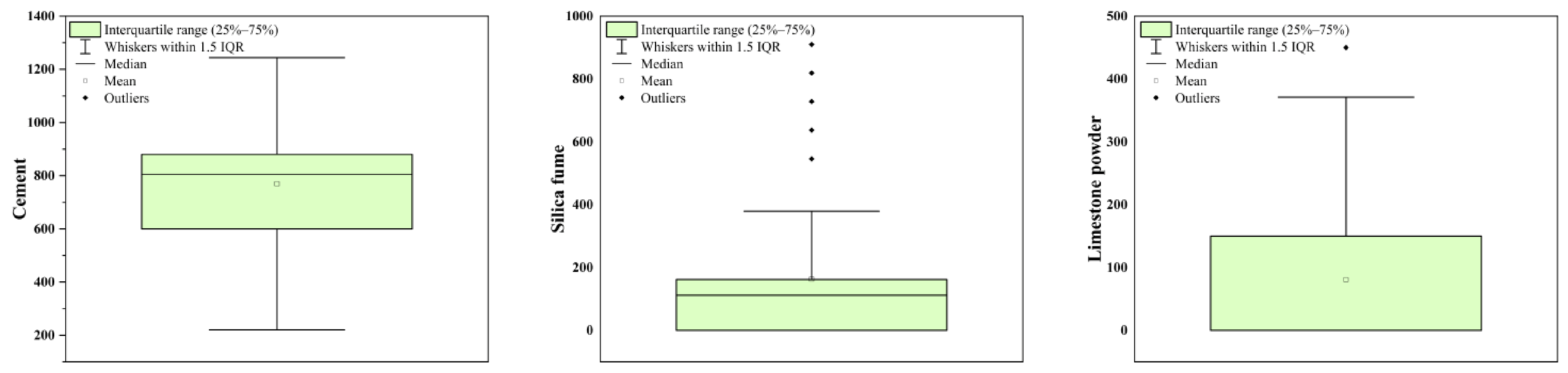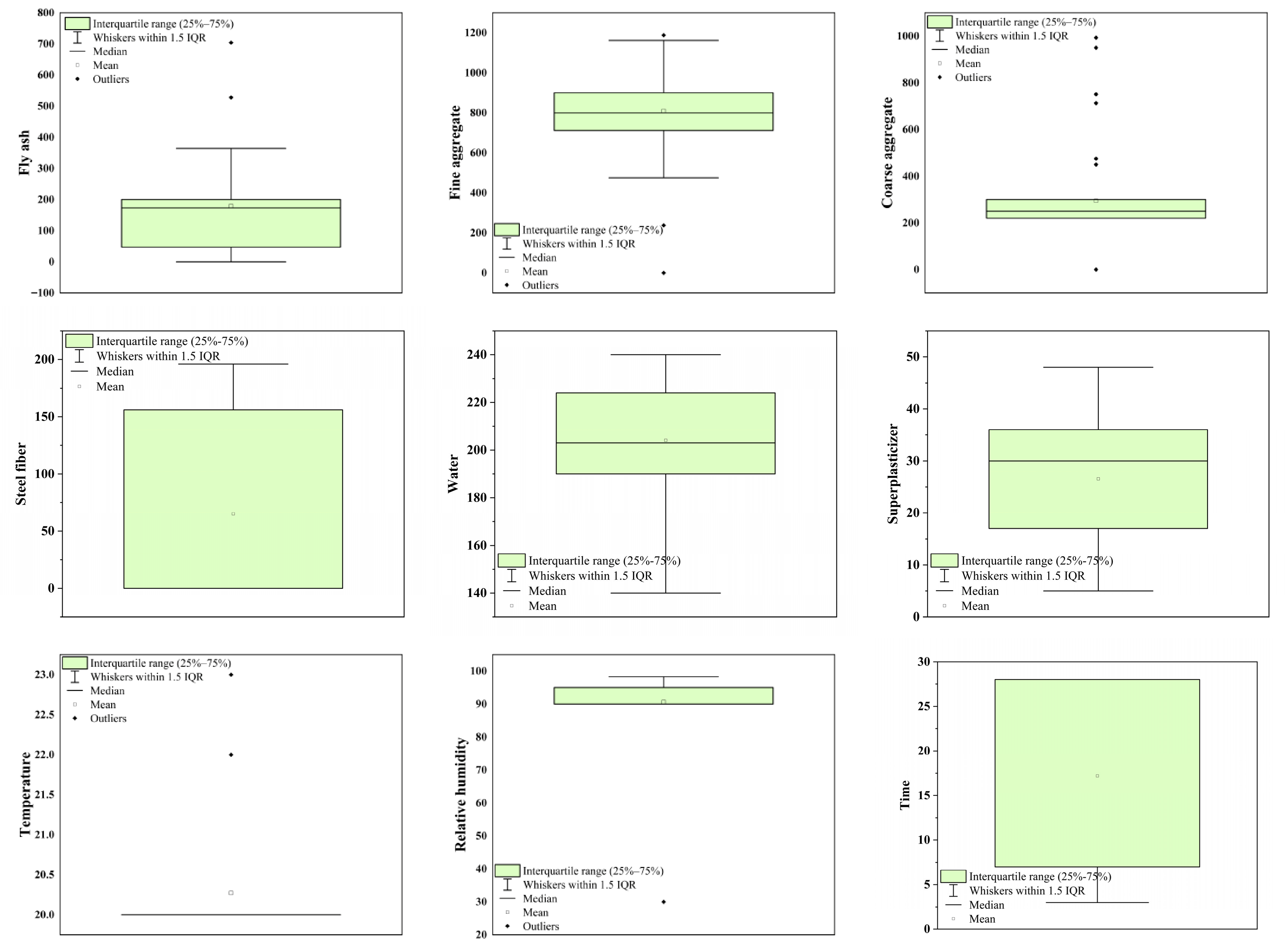The presence of such values may adversely affect data-driven models in two main ways: (1) they may increase error variance and reduce model fitting performance; (2) if caused by recording or matching problems, they may distort the statistical characteristics of the dataset [32]. However, in material datasets such as UHPC, extreme values are not necessarily erroneous and may instead correspond to physically meaningful boundary cases. Therefore, in this study, outlier handling was limited to screening and verification rather than automatic replacement. Potentially abnormal values were first flagged using the Interquartile Range (IQR) method (Figure 1).

The IQR is a quantile-based statistical approach that is robust to skewed distributions and can effectively identify values lying outside the main body of the data distribution. As a measure of statistical dispersion, quartiles partition a ranked dataset into four equal parts: Q₁ (first quartile), Q₂ (second quartile/median), and Q₃ (third quartile). The IQR is defined as the difference between the third and first quartiles.

$$IQR=Q_3-Q_1$$

(1)

Data points located beyond the upper bound (Q₃ + 1.5 × IQR) or below the lower bound (Q₁ − 1.5 × IQR) were flagged as potentially abnormal values for subsequent verification. Each IQR-flagged record was then manually checked against the original source article to determine whether the abnormal value resulted from a data-entry error, a unit-conversion inconsistency, or an ambiguous sample-matching issue. Only records with clear evidence of inconsistency were corrected or excluded; otherwise, physically plausible extreme values were retained in the final dataset. In this way, the IQR method was used as a screening tool for data verification rather than as a basis for automatic value replacement.

(C)

Data Normalization

Data normalization is a pivotal step in data preprocessing for machine learning. It aims to scale data proportionally within a specific narrow range, enabling the transformation of data with different magnitudes, units, or ranges into a unified set of standard numerical values for comparative analysis and weighting [33]. This process prevents features with larger numerical ranges from exerting disproportionate influence on the model’s performance. While tree-based models generally do not require normalization as they are not reliant on feature distances or magnitudes, and pre-normalized datasets do not require further processing, other deep learning architectures benefit significantly from this scaling [34].

Since the characteristics of UHPC do not strictly follow a normal distribution, the application of Z-score standardization is inappropriate for this study. Given that the dataset consists of non-normally distributed or bounded data, Min–Max normalization was employed to scale the data into a designated range, typically [0, 1]. Reference [35] as expressed in Equation (2).

$$x^{\prime }={\displaystyle \frac{x-\min (x)}{\max (x)-\min (x)}}$$

(2)

where $x$ represents the original data value; $min\left(x\right)$ and $max\left(x\right)$ are the minimum and maximum values of the feature, respectively; and $x^{\prime }$ is the normalized value.

(D)

Data Partitioning

To ensure model generalization and reduce the risk of overfitting, the dataset was randomly divided into a training set (70%), a validation set (15%), and an independent test set (15%). Hyperparameter tuning was conducted only within the training set using 5-fold cross-validation. Specifically, the training set was divided into five folds, and in each iteration, four folds were used for model fitting while the remaining fold was used for internal cross-validation. After the optimal hyperparameter configuration was determined, the model was retrained on the full training set. The separate validation set was then used for early stopping and checkpoint selection. Finally, the independent test set, which was not involved in training or model selection, was used exclusively for final performance evaluation.

2.3. Vae-Based Data Augmentation

The original dataset contains only 139 valid UHPC records, which is insufficient to support robust deep learning for synchronized multi-target prediction. To address this small-sample limitation, a Variational Autoencoder (VAE) [36] was introduced as a latent-space data-augmentation method prior to downstream model training. Unlike simple resampling or noise-based perturbation, the VAE learns the underlying distribution of the original dataset and generates synthetic samples that remain structurally consistent with the source data. In this way, the VAE improves feature-space coverage and provides more informative training data for the subsequent joint prediction of compressive strength, flexural strength, yield stress, and plastic viscosity.

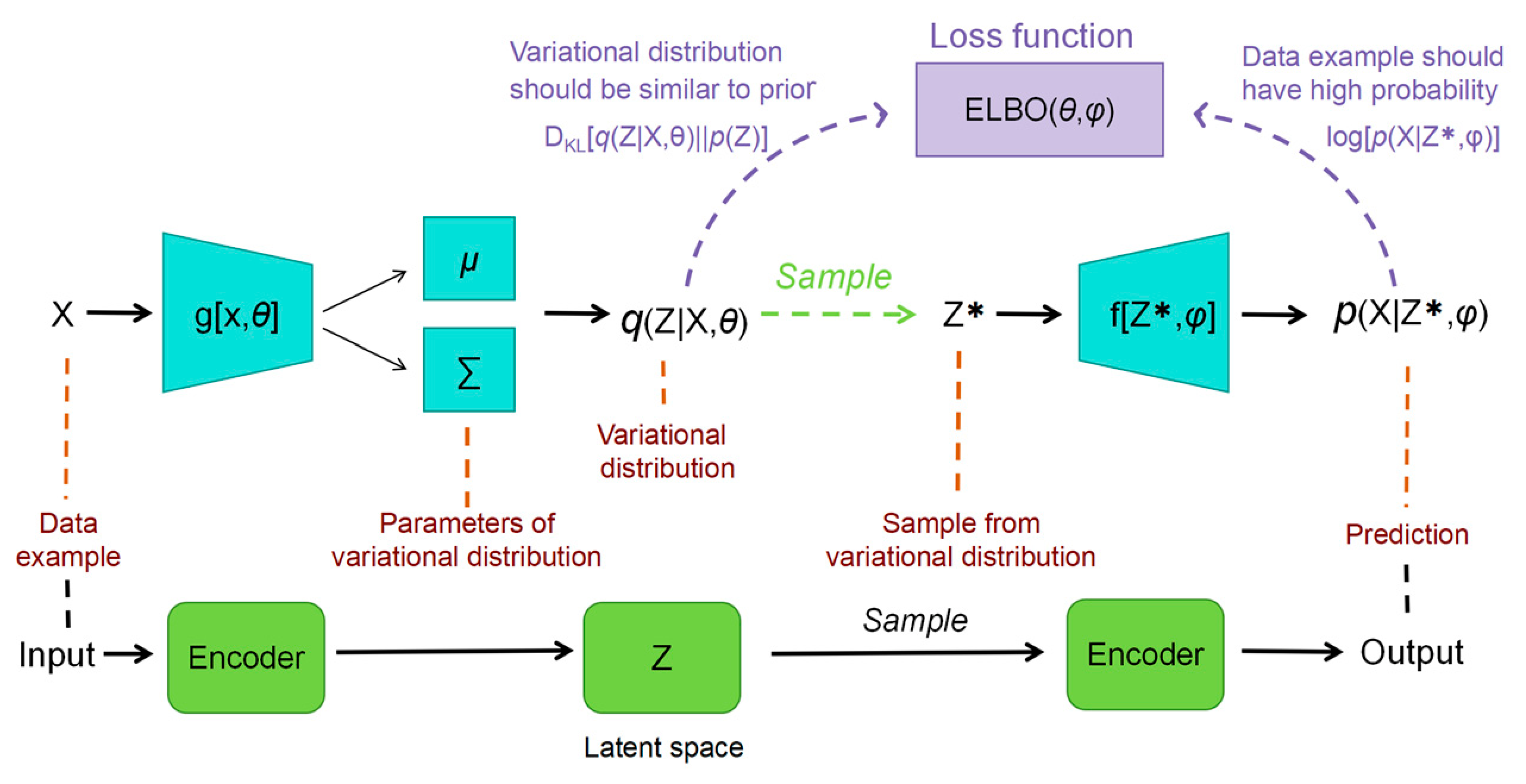
The data augmentation process used in this study is illustrated in Figure 2. The core mechanism of the VAE involves approximating the posterior distribution $p(z|x)$ through variational inference and optimizing the model parameters. Assuming the data x is generated by a latent variable z, the generative model can be represented as $p(x|z^{\ast })$. However, since $p(z|x)$ is mathematically intractable to solve directly, the VAE introduces an approximate distribution $q(z|x)$. The optimization objective is to make $q(z|x)$ as close as possible to the true posterior $p(z|x)$. This is achieved by minimizing the Kullback–Leibler (KL) Divergence between the two distributions, as shown in Equation (2).

$$KL(q(z|x)|| p(z|x))={\displaystyle \int q(z|x)\log \frac{q(z|x)}{p(z|x)}}dz$$

(3)

Through theoretical derivation, optimizing the KL divergence is equivalent to maximizing the Evidence Lower Bound (ELBO). As shown in Equation (4), since the KL divergence is non-negative, maximizing the ELBO serves as a proxy for approximating $\log p(x)$. The expression for the ELBO is provided in Equation (5).

$$\log p(x)=ELBO+KL(q(z|x)\left|\right| p(z|x))$$

(4)

$$ELBO={\mathrm{E}}_{q(z|x)}[\log p(x|z^{\ast })]-KL(q(z|x)|| p(z))$$

(5)

where $E_{q(z|x)}[\log p(x|z^{\ast })]$ represents the reconstruction error, signifying the log-likelihood expectation of reconstructing x from z; $KL(q(z|x)\left|\right| p(z))$ serves as the regularization term.

To enable model optimization via gradient descent, the VAE employs the reparameterization trick. Assuming $q(z|x)=N(\mu ,{\sigma }^2)$, direct sampling of $z~q(z|x)$ is non-differentiable. However, it can be rewritten as shown in Equation (6), where $\epsilon$ is random noise from a standard normal distribution, and $\mu ,\sigma$ are parameters output by the encoder.

$$z=\mu +\sigma \cdot \epsilon ,\epsilon ~N(0,I)$$

(6)

The calculation for the KL divergence regularization term in the loss function is given in Equation (7).

$$KL(N(\mu ,{\sigma }^2)|| N(0,I)={\displaystyle \frac{1}{2}}{\displaystyle \sum (1+\log {\sigma }^2-{\mu }^2}-{\sigma }^2)$$

(7)

In practice, the encoder takes input x and outputs $\mu$ and $\log {\sigma }^2$, generating z through reparameterization. The decoder then takes z as input to output the distribution parameters of the reconstructed $\stackrel{⌢}{x}$.

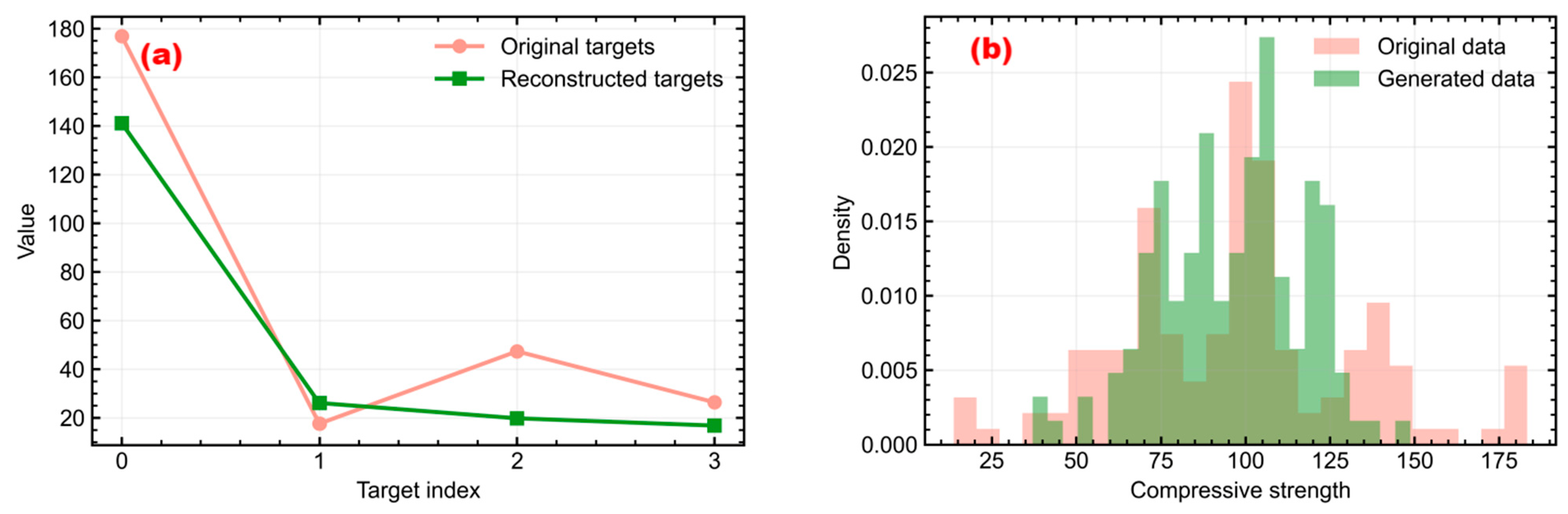
Following the optimization and training of the VAE model, a synthetic dataset 20 times the size of the original sample was generated, resulting in 2780 new UHPC mix proportion data points. As illustrated in Figure 3, the VAE model demonstrates exceptional performance in data reconstruction. Figure 3a takes compressive strength as a representative example; the overall trends of the original and reconstructed data are highly consistent, indicating that the model effectively captures the primary features of the dataset and achieves precise reconstruction. Furthermore, as shown in Figure 3b, the distribution of the newly generated UHPC compressive strength data more closely approximates a normal distribution while maintaining the fundamental distribution characteristics of the original data. This further validates the rationality and reliability of the data generated by the model.

2.4. Multi-Target Deep Learning Model

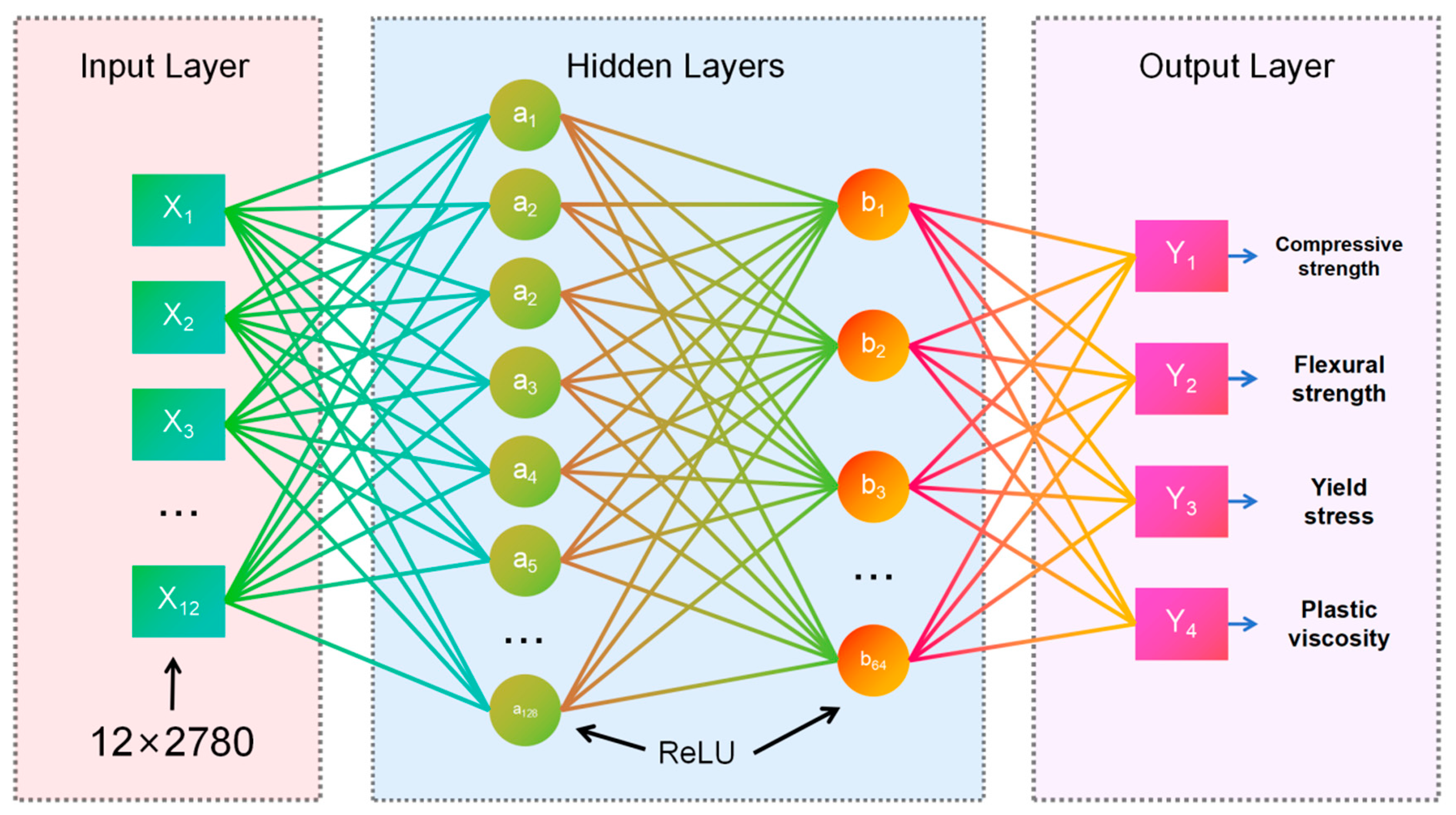
In this study, a Deep Neural Network (DNN) model was trained and optimized based on the TensorFlow framework to predict four target output variables (Figure 4). The neural network architecture comprises an input layer, two hidden layers, and an output layer. The input layer consists of 12 dimensions corresponding to the input parameters. Hidden Layer 1 contains 128 neurons activated by the ReLU function, while Hidden Layer 2 contains 64 neurons, also employing ReLU activation. The output layer consists of 4 neurons with linear activation to facilitate regression.

In addition to the network architecture, the training objective of the proposed multi-output DNN was defined as the weighted sum of four task-specific Huber losses corresponding to compressive strength, flexural strength, yield stress, and plastic viscosity. Let $y_{i,t}$ and ${\widehat{y}}_{i,t}$ denote the true and predicted values of sample $i$ for target $t$ respectively, where $i\in \{1,2,3,4\}$. The overall multi-target loss was formulated as Equation (8).

$${\mathrm{L}}_{\mathrm{total}}={\displaystyle \sum _{t=1}^4{\lambda }_t}{L}_{Huber}^{(t)}$$

(8)

where ${\lambda }_t$ denotes the loss weight assigned to task $t$. For each target, the Huber loss was defined as Equation (9).

$$L_{Huber}^{(t)}={\displaystyle \frac{1}{N}}{\displaystyle \sum _{i=1}^N\left\{\begin{array}{l}\frac{1}{2}{\left(y_{i,t}-{\widehat{y}}_{i,t}\right)}^2,if\left|y_{i,t}-{\widehat{y}}_{i,t}\right|\le \delta \\ \delta \left|y_{i,t}-{\widehat{y}}_{i,t}\right|-\frac{1}{2}{\delta }^2,\left|y_{i,t}-{\widehat{y}}_{i,t}\right|\ge \delta \end{array}\right.}$$

(9)

To enhance predictive accuracy, the model was trained using the Adam (Adaptive Moment Estimation) optimizer. The Adam algorithm integrates the advantages of Momentum and RMSProp (Root Mean Square Propagation), accelerating the convergence of gradient descent by adaptively adjusting the learning rate. While Adam exhibits robust performance in tasks involving large-scale data and high-dimensional parameter spaces, it may not always converge to the global optimum; in certain non-convex optimization problems, it may converge to a sub-optimal solution. Furthermore, the algorithm is sensitive to hyperparameters; although the default values are widely applicable, fine-tuning is often necessary for specific tasks.

Mechanistically, Adam dynamically adjusts the learning rate for each parameter by utilizing estimates of the first-order moment and the second-order moment. These two moment estimates help mitigate common deficiencies in standard Stochastic Gradient Descent (SGD), such as slow convergence or excessive oscillations.

For each parameter $\theta$, the Adam algorithm maintains two estimates: the first-order moment m_t and the second-order moment v_t. Prior to training, the model parameters must be initialized. The specific parameters and their corresponding physical significances are summarized in

Table 2. Initialization of Adam Algorithm Parameters and Their Physical Significance.

Parameter	Significance
${\theta }_0$	Initialized model parameters.
$m_0=0$	Initialized first-order moment (momentum) set to 0.
$v_0=0$	Initialized second-order moment (uncentered variance of gradients) set to 0.
${\beta }_1$	Exponential decay rate for the first-order moment (typically set to 0.9).
${\beta }_2$	Exponential decay rate for the second-order moment (typically set to 0.999).
$\alpha$	Learning rate (typically set to 0.001).
$\epsilon$	A small constant (typically set to 10−8 to prevent division by zero errors.

.

For each iteration of the training process, the gradient of the current parameters is first calculated as shown in Equation (10), where $f({\theta }_t)$ represents the objective function (typically the loss function). Subsequently, the first-order momentum and second-order moment (uncentered variance of gradients) are updated according to Equations (11) and (12). The momentum represents the accumulation of historical gradient information through an exponentially weighted moving average. The second-order moment estimates the variance of the gradients, which assists in adjusting the learning rate for each parameter.

$$g_t={\nabla }_{\theta }f({\theta }_t)$$

(10)

$$m_t={\beta }_1{m}_{t-1}+(1-{\beta }_2)g_t$$

(11)

$$v_t={\beta }_2{v}_{t-1}+(1-{\beta }_2){g_t}^2$$

(12)

Since the initial estimates of $m_t$ and $v_t$ are biased toward zero at the start of training, bias correction is performed to bring them closer to the true gradient estimates. The corrected moments are calculated as shown in Equations (13) and (14), where $t$ denotes the current time step.

Finally, the parameters are updated using the corrected momentum and variance estimates (Equation (15)), where $\sqrt{{\stackrel{⌢}{v}}_t}+\epsilon$ ensures numerical stability and prevents division-by-zero errors.

$${\stackrel{⌢}{m}}_t={\displaystyle \frac{m_t}{1-{\beta }_1^t}}$$

(13)

$${\stackrel{⌢}{v}}_t={\displaystyle \frac{v_t}{1-{\beta }_2^t}}$$

(14)

$${\theta }_{t+1}={\theta }_t-{\displaystyle \frac{\alpha {\widehat{m}}_t}{\sqrt{{\widehat{v}}_t}+\epsilon }}$$

(15)

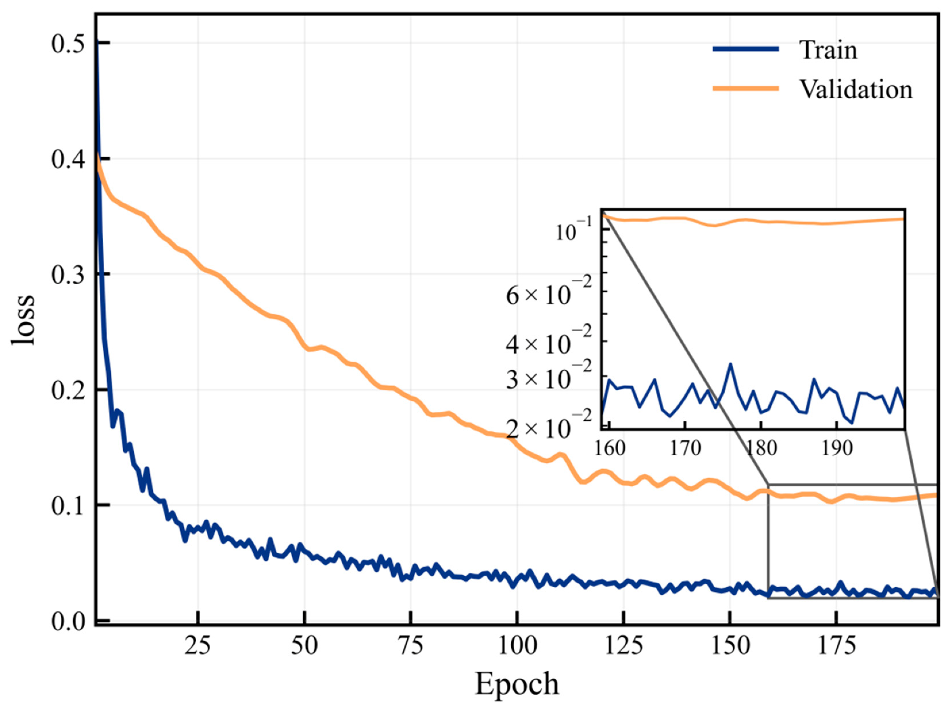
As illustrated by the training curves in Figure 5, the model exhibits stable convergence throughout the training process. The training loss decreases sharply within the initial epochs, followed by a phase of gradual attenuation, ultimately reaching a plateau after approximately 150 epochs. Similarly, the validation loss continues to decline and stabilizes at a low level in the later stages. Minor fluctuations observed between 160 and 200 epochs without any systematic upward trend indicate that the model has reached convergence while maintaining consistent generalization performance. Although the training loss remains consistently lower than the validation loss, representing a characteristic generalization gap, the validation curve does not rebound, suggesting that no significant overfitting occurred during the training process.

2.5. Benchmark Architectures and Comparative Protocol

To assess whether the performance of the proposed framework arises from architectural design or from the overall small-sample learning pipeline, three representative benchmarks were introduced: (1) single-task DNNs trained separately for each target, (2) a shared-trunk multi-task network with task-specific heads, and (3) an attention-based multi-task model. For fair comparison, all benchmark models were trained using the same input variables, output targets, data split, optimizer, batch size, early-stopping strategy, and evaluation metrics as the proposed model.

2.6. Model Evaluation Metrics

Model evaluation is an essential step in machine learning, as it quantifies predictive capability and verifies whether a trained model satisfies the expected performance requirements. A well-designed evaluation scheme assesses not only accuracy but also generalization and robustness, thereby helping to identify overfitting or underfitting. Since this study focuses on regression problems, commonly used regression metrics are briefly introduced and used to compare model performance in a consistent manner. The evaluation metrics adopted in this paper are summarized in

Table 3. Regression Model Evaluation.

	Symbol	Formulas	Ideal Value
R-squared	R2	$R^2=1-{\displaystyle \frac{{\displaystyle \sum _{i=1}^{\mathrm{m}}{(p_i-T_i)}^2}}{{\displaystyle \sum _{i=1}^m(p_i-\overline{T}{)}^2}}}$	R2 = 100%
Mean Absolute Error	MAE	$MAE={\displaystyle \frac{{\displaystyle \sum _{i=1}^m\left|p_i-T_i\right|}}{m}}$	MAE = 0
Root Mean Squared Error	RMSE	$RMSE=\sqrt{{\displaystyle \frac{{\displaystyle \sum _{i=1}^m{(p_i-T_i)}^2}}{m}}}$	RMSE = 0
Mean Squared Error	MSE	$MSE={\displaystyle \frac{{\displaystyle \sum _{i=1}^m{(p_i-T_i)}^2}}{m}}$	MSE = 0

Note: where $T_i$ is the true value, $P_i$ is the predicted value, $i=1,2,3,\dots ,m$ is the sample index, and $\overline{T}$ is the average true value of the samples.

.

2.7. Interpretability Analysis Using SHAP and PDP

To improve the interpretability of the proposed multi-output deep learning model, SHAP (SHapley Additive exPlanations) and Partial Dependence Plots (PDP) were employed to analyze the relationships between input variables and predicted UHPC properties. SHAP is a model-agnostic interpretability framework that explains individual predictions by assigning each feature an additive contribution value. By evaluating the marginal contribution of each feature across different feature combinations, SHAP provides a mathematically consistent attribution scheme and is therefore well suited for interpreting complex ‘black-box’ models. Its flexibility enables both local and global interpretation for a wide range of predictive models, including deep learning architectures. In this study, SHAP was used to quantify the relative importance and directional influence of input variables on the four target outputs, thereby improving model transparency and facilitating mechanism-oriented interpretation.

The SHAP framework unifies previously proposed interpretability methods, such as LIME and DeepLIFT, under the umbrella of additive feature attribution methods [37]. These methods employ an explanation model defined as a linear function of simplified binary variables, as expressed in Equation (14), where $f(x)$ represents the original model, $g(x)$ is the explanation model, $z_i$ in {0, 1} denotes the simplified input, $m$ is the number of input features, and ${\phi }_0$ is a constant. For machine learning models where all features of sample X are present, Equation (16) simplifies to Equation (17).

$$f(x)=g(z)={\phi }_0+{\displaystyle \sum _{i=1}^m{\phi }_i}{z}_i$$

(16)

$$g(z)={\phi }_0+{\displaystyle \sum _{i=1}^m{\phi }_i}$$

(17)

For linear regression models, Equations (18) and (19) define the predictive contribution of the $i$ feature, where $p$ is the number of features, $\beta$ represents the feature weights, and $E({\beta }_i{x}_i)$ is the estimated average influence of feature $i$.

$$\beta \hspace{1em}\widehat{f}(x)={\beta }_0+{\beta }_{1}x+\cdots +{\beta }_p{x}_p$$

(18)

$${\phi }_i={\beta }_i{x}_i-E({\beta }_i{x}_i)={\beta }_i{x}_i-{\beta }_{i}E(x_i)$$

(19)

Summing the contribution values of all features for a specific sample equals the difference between the predicted value and the average prediction, as shown in Equation (20). This relationship holds for linear models with independent features but is inapplicable to non-linear models like tree-based ensembles. To determine the contribution of a specific feature $i$ in such cases, the Shapley value is calculated by evaluating all possible feature combinations and computing a weighted sum, as expressed in Equation (21).

$$\begin{array}{ll}{\displaystyle {\displaystyle \sum _{i=1}^p}{\varphi }_i}(\widehat{f})& ={\displaystyle {\displaystyle \sum _{i=1}^p}({\beta }_i{x}_i}-E({\beta }_i{X}_i))\\ & =({\beta }_0+{\displaystyle {\displaystyle \sum _{i=1}^p}({\beta }_i}{X}_i))-({\beta }_0+{\displaystyle {\displaystyle \sum _{i=1}^p}E({\beta }_i}{X}_i))\\ & =\overline{f}(x)-E(\overline{f}(X))\end{array}$$

(20)

$${\phi }_i(val)={\displaystyle \sum _{S\subseteq \{x_1,\cdots ,x_p\}\backslash \left\{x_i\right\}}\frac{\left|S\right|!(p-|S|-1)!}{p!}}(val(S\cup \{x_i\}-val(S))$$

(21)

where $S$ is a subset of features, $x$ is the feature vector, and $val(S)$ is the output for a given feature combination. From a weighting perspective, there are $p!$ possible permutations for $p$ features. By fixing a specific feature $j$, there are $(p-|S|-1)!$ remaining combinations. To isolate the pure interaction effect, the main effects of each feature should be subtracted from the total contribution. This yields a more precise individual effect and interaction analysis, as shown in Equation (22).

$${\delta }_{ij}(S)=f_x(S\cup \{i,j\})-f_x(S\cup \{j\})+f_x(S)$$

(22)

Furthermore, Partial Dependence Analysis (PDA) serves as a visualization tool to interpret model behavior by examining the marginal effect of individual features on the predicted outcome. PDA focuses on specific features by fixing their values to mitigate the complexity of the high-dimensional feature space. Given a prediction model $f$ and feature vector $X=\left\{X_1,X_2,\dots ,X_p\right\}$, the partial dependence function for a specific subset $S\subseteq \left\{1,2,\dots ,p\right\}$ is defined in Equation (23).

$$P{D}_S(x_S)=E_{X_C}[f(x_S,X_C)]$$

(23)

where $x_S$ represents the features in $S$, $X_C$ denotes the remaining features, and $E_{X_C}$ is the expectation over the conditional distribution of $X_C$.

3. Results and Discussion

3.1. Prediction Performance

This study presents a comprehensive performance evaluation of the VAE-enhanced deep learning model across four predictive targets: compressive strength (MPa), flexural strength (MPa), yield stress (Pa), and plastic viscosity (Pa·s). Quantitative assessments were conducted using R², RMSE, and MAE for the training, validation, and testing datasets (

Table 4. Performance evaluation of the deep learning models.

Target	Unit	Training Dataset			Validation Dataset			Test Dataset
		R2	RMSE	MAE	R2	RMSE	MAE	R2	RMSE	MAE
Compressive strength	MPa	0.977	3.212	2.374	0.866	14.403	8.092	0.950	8.021	5.057
Flexural strength	MPa	0.976	0.898	0.682	0.747	5.186	3.350	0.895	3.285	2.402
Yield stress	Pa	0.968	4.878	3.586	0.773	16.350	12.626	0.888	13.709	10.571
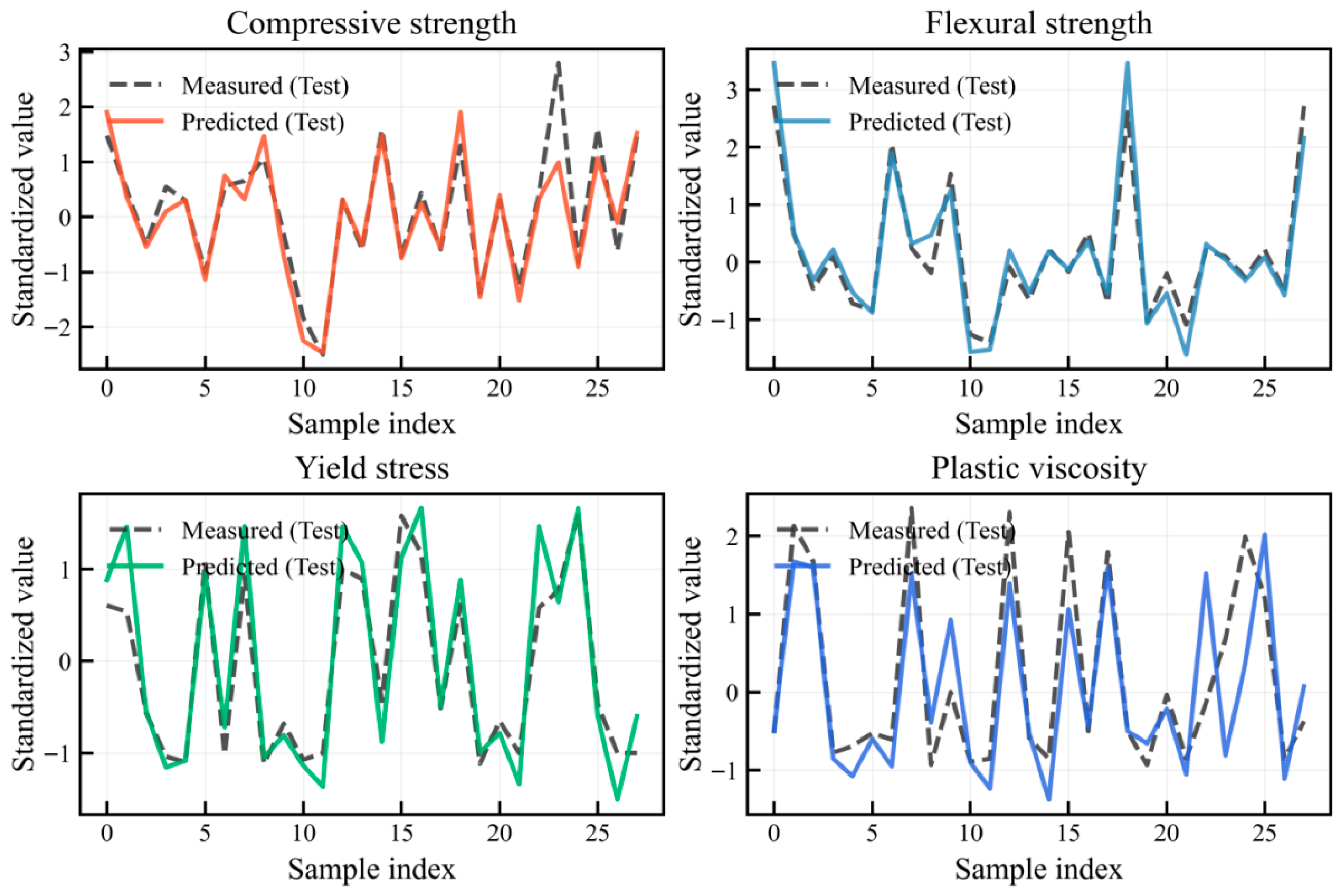
Plastic viscosity	Pa·s	0.958	3.066	2.020	0.532	12.659	8.668	0.689	15.243	11.277

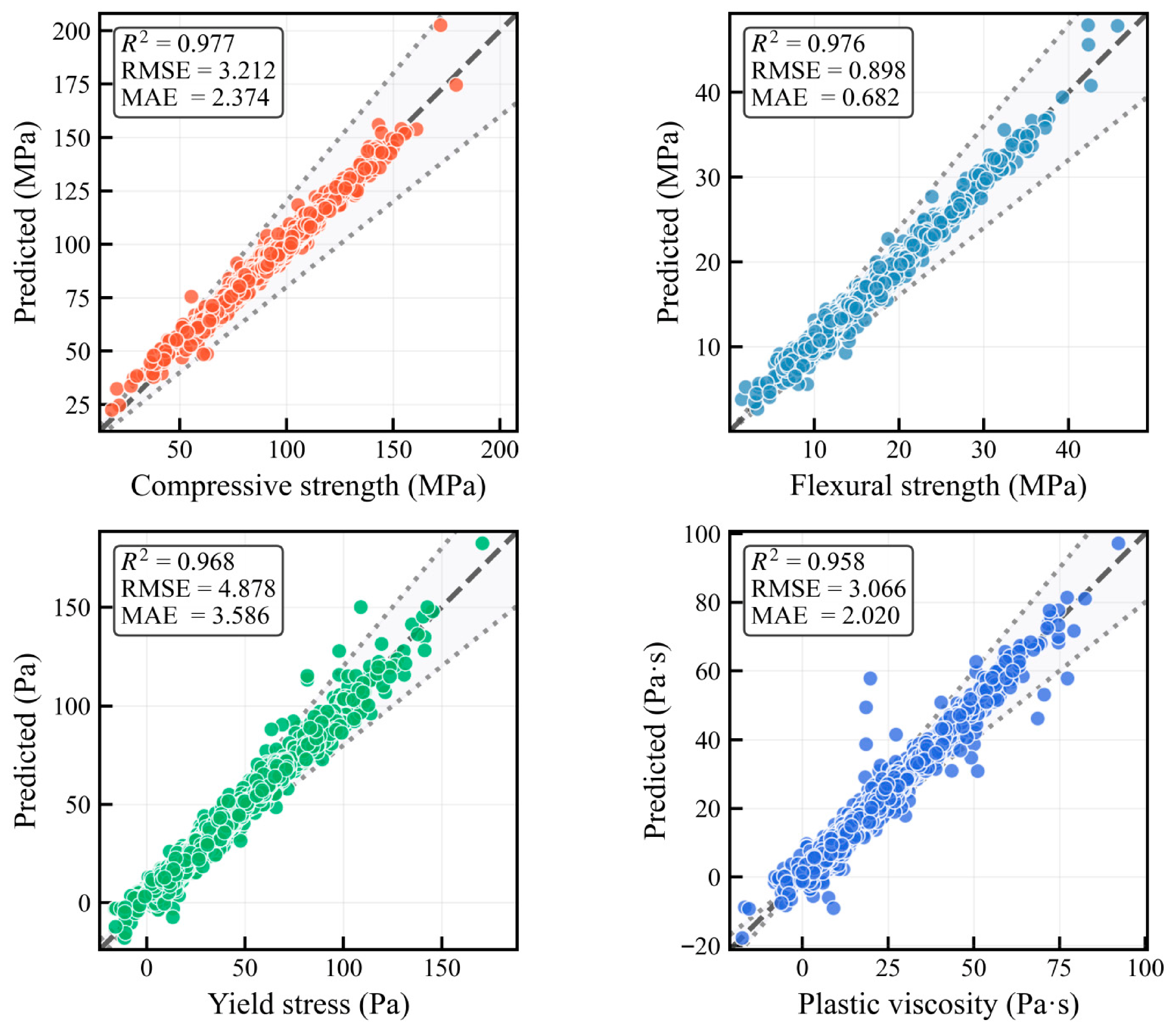
). Furthermore, visualization analysis was performed by comparing normalized sequences (Figure 6) and predicted-versus-measured consistency scatter plots (Figure 7) specifically for the testing set.

As summarized in Table 4, the model exhibits high fitting accuracy on the training set, with R² values for the four targets reaching 0.977, 0.976, 0.968, and 0.958, respectively. The corresponding RMSE/MAE values are 3.212/2.374 MPa (compressive strength), 0.898/0.682 MPa (flexural strength), 4.878/3.586 Pa (yield stress), and 3.066/2.020 Pa·s (plastic viscosity). Figure 7 illustrates that during the training phase, the predicted data points generally align closely with the 1:1 diagonal line. While the strength-related indicators show lower dispersion, the viscosity-related indicators exhibit slightly higher variance, though the overall trends remain consistent.

A relative decrease in accuracy is observed in the validation set (R² = 0.866, 0.747, 0.773, and 0.532), accompanied by increased error metrics. This performance discrepancy between training and validation suggests potential distributional shifts or more complex sample intervals within the validation set. Specifically, plastic viscosity appears more sensitive to raw material variations or mix proportions, leading to higher predictive uncertainty.

On the independent test set, strength-related metrics maintain robust generalization capability: compressive strength achieved an R² of 0.950 (RMSE = 8.020 MPa, MAE = 5.057 MPa), and flexural strength reached an R² of 0.895 (RMSE = 3.285 MPa, MAE = 2.402 MPa). Yield stress also performed well with an R² of 0.888. In contrast, the plastic viscosity in the test set yielded a lower R² of 0.689 and larger errors, indicating that its prediction remains more challenging. In Figure 6, the normalized prediction curves successfully track the peak-and-valley fluctuations of the experimental data, demonstrating the model’s capacity to characterize relative variations between samples. However, local deviations are more pronounced for viscosity, which is consistent with the error analysis in Table 4.

3.2. Inter-Target Relationships Among the Four Prediction Targets

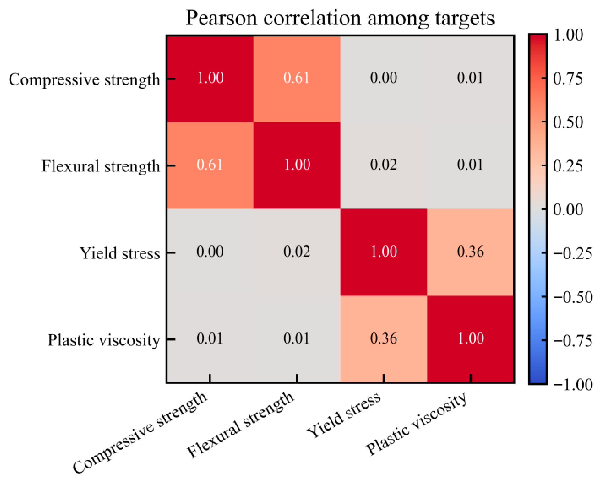
To quantify the relationships among the four jointly predicted targets, Pearson correlation analysis was conducted, as shown in Figure 8. The results indicate a moderate positive correlation between compressive strength and flexural strength (r = 0.61), and a weaker but still positive correlation between yield stress and plastic viscosity (r = 0.36). In contrast, the cross-group correlations between strength-related and rheology-related targets are generally weak, suggesting a nonuniform dependency structure across tasks.

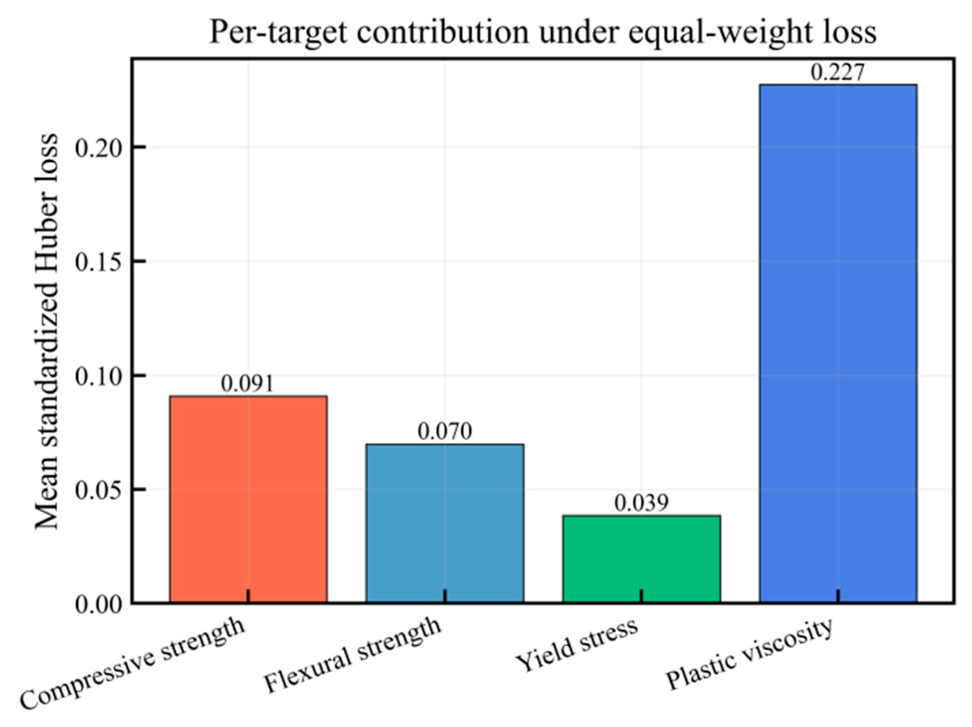
In addition, the per-target contribution under the equal-weight loss setting is shown in Figure 9. Since all target variables were standardized before model training, equal loss weights were assigned to all tasks in the multi-task objective, rather than manually tuned weights. Although all targets were optimized under the same loss setting, the task-wise standardized Huber loss contributions remain uneven. In particular, plastic viscosity exhibits the largest loss contribution, indicating that it is the most difficult target to optimize in the present multi-task framework. This suggests that equal weighting alleviates scale-induced dominance but does not fully eliminate task imbalance.

3.3. Error Diagnostics and Learning Behavior

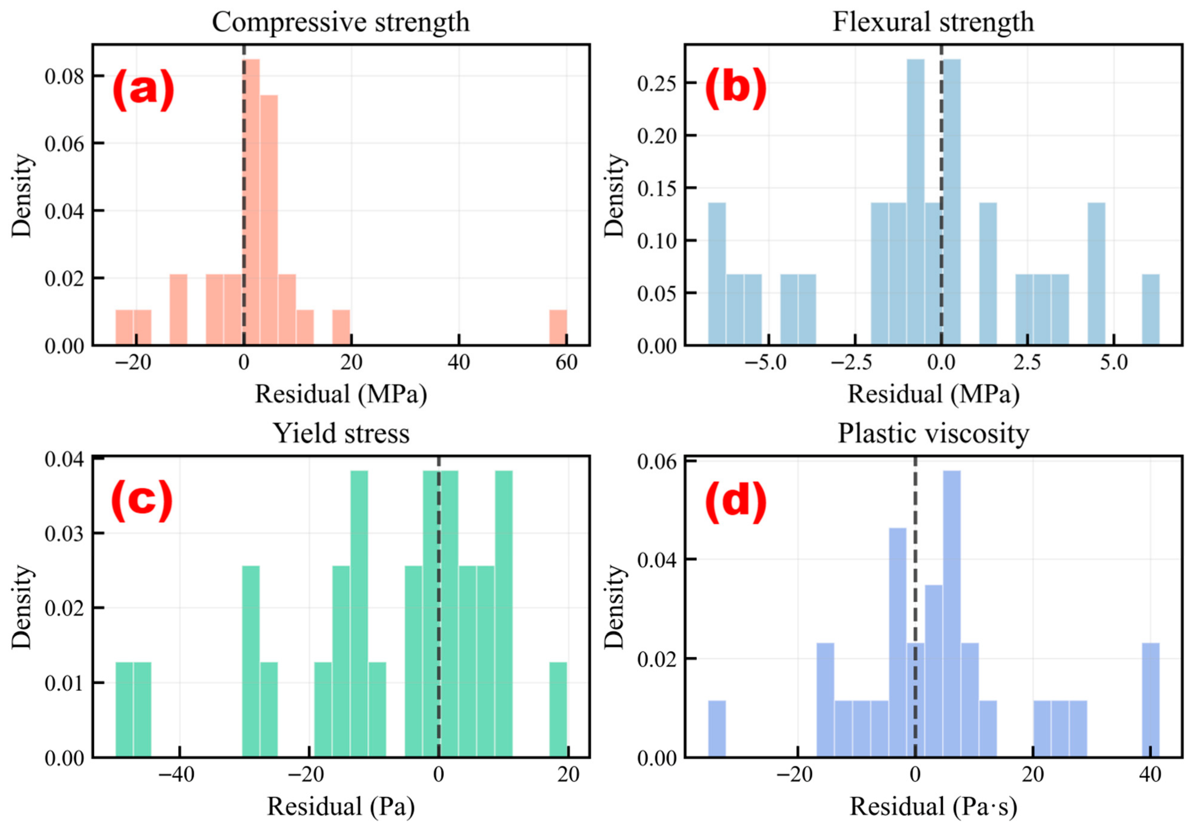
To elucidate the sources of error underlying the overall performance metrics, the residual distributions are presented in Figure 10. The residual is defined as e = y_pred − y_meas, where the dashed lines in the figure represent the zero-residual baseline.

As illustrated in Figure 10a,b, the residuals for compressive strength and flexural strength are primarily concentrated around zero, indicating that the overall predictive bias remains well-controlled. The flexural strength exhibits a narrower residual distribution, corresponding to a more stable error level. In contrast, the compressive strength displays a broader distribution with a distinct long-tail effect, suggesting that a small subset of samples contributes disproportionately to the error, thereby inflating the RMSE. Regarding yield stress and plastic viscosity, Figure 10c,d reveal further expansion of the residuals with even heavier tails. This signifies a higher error variance and a greater dominance of extreme samples in the total error profile. Notably, the tail for plastic viscosity is the most prominent, identifying it as the output parameter that is most challenging for the current model to constrain effectively.

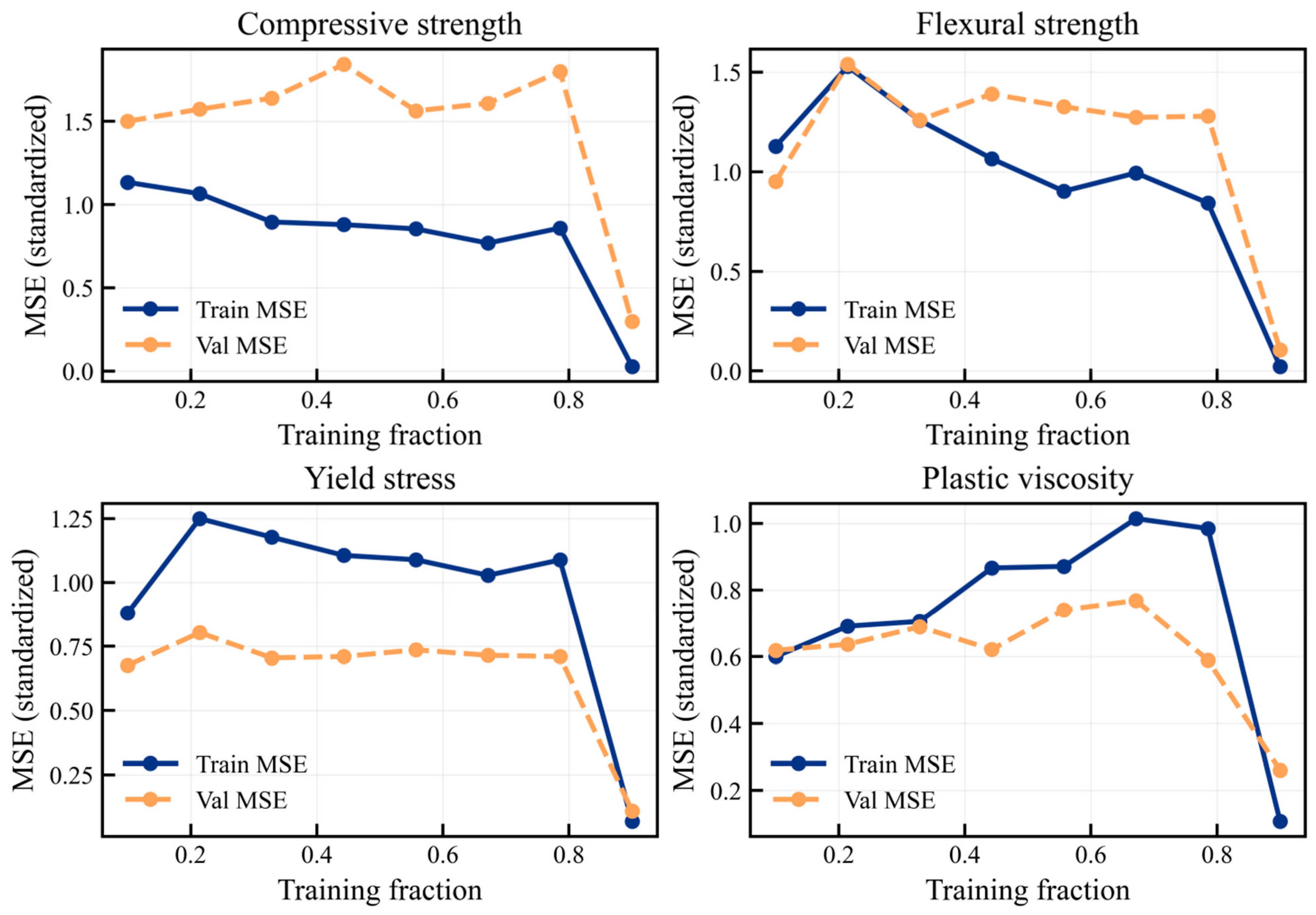
Figure 11 illustrates the variations in normalized Mean Squared Error (MSE) for both the training and validation sets under different training fractions. The overall trend indicates that as the training fraction increases, the training error generally declines, suggesting that the model continuously improves its fitting capacity by learning from a larger sample size. Similarly, the validation error follows a downward trajectory but at a more gradual pace, maintaining a persistent gap with the training error over a substantial range. This discrepancy reflects a certain generalization gap inherent to the model under limited data conditions.

Regarding target-specific performance, the training–validation gap is more pronounced for compressive strength and plastic viscosity, indicating that their underlying mapping relationships are more complex and highly sensitive to sample coverage and feature representation. In contrast, the validation error curve for yield stress remains relatively stable, implying a higher degree of learnability for this target within the current feature set. A significant drop in error at higher training fractions underscores the model’s strong data dependency; as data coverage expands, the model’s ability to fit and generalize to boundary samples within the distribution improves markedly.

In summary, the model error is primarily driven by a small number of “long-tail samples”, a phenomenon most evident in plastic viscosity. To further enhance performance, future efforts should prioritize data augmentation and targeted sampling for these long-tail regions. Additionally, adopting training objectives that are more robust to outliers could effectively compress tail errors and narrow the training–validation gap.

3.4. Comparative Analysis Against Representative Multi-Task Architectures

Table 5. Comparative test-set performance of representative benchmark architectures for four-target UHPC prediction.

Model	Compressive Strength		Flexural Strength		Yield Stress		Plastic Viscosity
	R2	RMSE	R2	RMSE	R2	RMSE	R2	RMSE
Single-task DNN	0.842	16.689	0.878	4.601	0.815	21.339	0.665	15.562
Shared trunk + task-specific heads	0.800	19.539	0.857	4.989	0.833	19.772	0.534	23.667
Attention-based multi-task	0.843	16.598	0.849	5.122	0.847	18.199	0.578	22.386
multi-output DNN	0.860	13.362	0.921	2.845	0.846	16.067	0.660	15.928

compares the proposed multi-output DNN with three representative benchmark architectures on the independent test set for four-target UHPC prediction. Overall, the proposed model exhibited the most balanced and competitive generalization performance across the four targets. Specifically, it achieved the best performance for compressive strength and flexural strength, with the highest R² values (0.860 and 0.921) and the lowest RMSE values (13.362 and 2.845), respectively. For yield stress, although the attention-based multi-task model obtained a marginally higher R² value, the proposed model yielded a substantially lower RMSE, indicating better predictive accuracy in absolute terms. For plastic viscosity, the single-task DNN performed slightly better than the proposed model, suggesting that this target remains more challenging and may still benefit from task-specific modeling. Nevertheless, the proposed model maintained competitive performance while providing stronger overall balance across the four outputs. These results suggest that the predictive gains observed in this study are mainly associated with the joint-learning design of the multi-output DNN, while also reflecting the effectiveness of the overall data-driven framework.

3.5. Ablation Study on the Effect of VAE Augmentation

To isolate the specific contribution of VAE-based augmentation, an ablation study was conducted using four augmentation settings: no augmentation, random oversampling, Gaussian-noise augmentation, and VAE-based augmentation. In all cases, the downstream predictive architecture, optimizer, and training protocol were kept unchanged, and only the training-data generation strategy was varied. This design allows the performance differences to be attributed more directly to the augmentation strategy itself rather than to changes in model complexity or parameter count.

As shown in

Table 6. Comparative performance of benchmark architectures for four-target UHPC prediction.

Setting	Compressive Strength	Flexural Strength	Yield Stress	Plastic Viscosity
	R2
No_augmentation	0.928 ± 0.026	0.901 ± 0.124	0.915 ± 0.219	0.793 ± 0.248
Random_oversampling	0.917 ± 0.068	0.973 ± 0.098	0.958 ± 0.077	0.892 ± 0.241
Gaussian_noise	0.926 ± 0.037	0.956 ± 0.080	0.952 ± 0.135	0.840 ± 0.193
VAE_augmentation	0.981 ± 0.016	0.978 ± 0.009	0.973 ± 0.067	0.960 ± 0.169

, VAE-based augmentation achieved the best performance across all four prediction targets. Specifically, it yielded the highest R² values for compressive strength, flexural strength, yield stress, and plastic viscosity, reaching 0.981 ± 0.016, 0.978 ± 0.009, 0.973 ± 0.067, and 0.960 ± 0.169, respectively. In contrast, the other augmentation strategies produced lower predictive accuracy and generally larger variability across repeated runs. Random oversampling improved the prediction of flexural strength and yield stress relative to the non-augmented setting, while Gaussian-noise augmentation showed moderate gains for several targets. However, neither of these conventional augmentation strategies matched the overall performance of VAE-based augmentation.

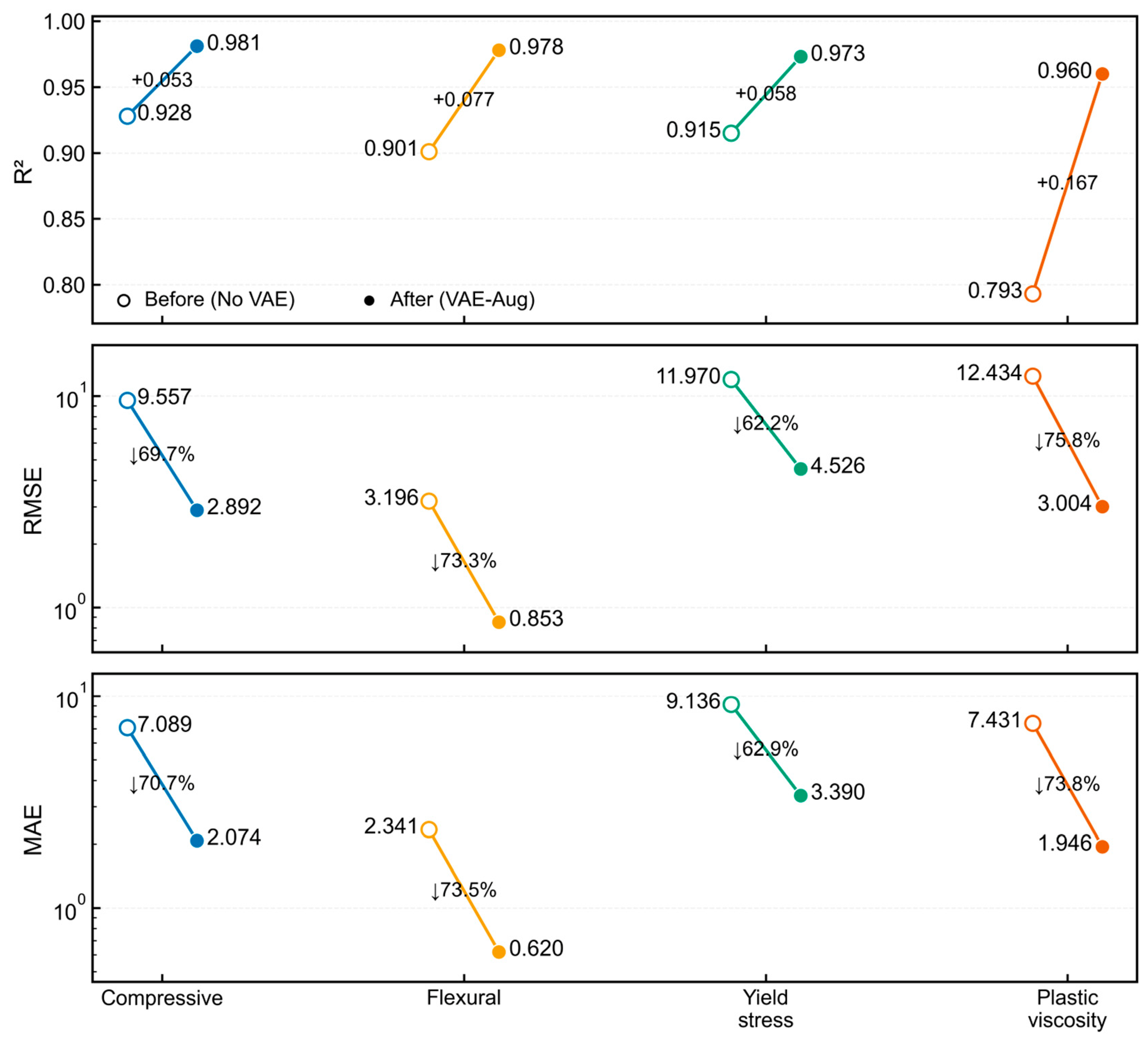
Furthermore, the authors compared the changes in key evaluation metrics before and after the introduction of the VAE, as illustrated in Figure 12. The results indicate that VAE augmentation exerted a consistent positive influence across all four target variables, enhancing the overall predictive performance of the model. Notably, the degree of optimization was particularly significant for error-based metrics, such as Root Mean Square Error (RMSE) and Mean Absolute Error (MAE).

In terms of goodness-of-fit, the R² values for all four targets improved significantly: compressive strength rose from 0.928 to 0.981 (+0.053), flexural strength from 0.901 to 0.978 (+0.077), yield stress from 0.915 to 0.973 (+0.058), and plastic viscosity from 0.793 to 0.960 (+0.167). The most substantial increase was observed in plastic viscosity, suggesting that generative augmentation provides greater benefits for targets characterized by high uncertainty and complexity.

Regarding error levels, VAE enhancement markedly reduced both RMSE and MAE (note that units for these metrics correspond to their respective targets: MPa for strength, Pa for yield stress, and Pa·s for viscosity). Specifically, the compressive strength RMSE dropped from 9.557 to 2.892 (a 69.7% reduction) and MAE from 7.089 to 2.074 (70.7% reduction). For flexural strength, the RMSE decreased from 3.196 to 0.853 (73.3% reduction) and MAE from 2.341 to 0.620 (73.5% reduction). Yield stress RMSE was reduced from 11.970 to 4.526 (62.2% reduction) and MAE from 9.136 to 3.390 (62.9% reduction). Finally, plastic viscosity showed an RMSE decrease from 12.434 to 3.004 (75.8% reduction) and MAE from 7.431 to 1.946 (73.8% reduction). These findings indicate that VAE enhancement not only enhances correlation (R²) but also substantially compresses absolute error levels, particularly for targets sensitive to data coverage, such as plastic viscosity and flexural strength.

These results indicate that the observed performance gains cannot be explained solely by increased sample size or simple perturbation-based data expansion. Instead, the superiority of the VAE-based strategy suggests that latent-space modeling provides more informative and better-structured synthetic samples, which improve data distribution coverage and enhance generalization under small-sample conditions. Therefore, VAE augmentation plays a substantive role in the proposed framework and is an important contributor to its predictive effectiveness.

3.6. Explainability Results

To enhance model transparency, this study utilizes SHAP to interpret and analyze the four predictive targets on the test set. Given that the output variables were standardized during the training and evaluation phases, the SHAP values reported herein reside within the standardized output space. Specifically, a positive SHAP value indicates that a feature drives the model output upward, whereas a negative value indicates a downward pull. These attribution results are intended to characterize the relative contribution structure of the model and should not be interpreted as direct causal effects measured in physical units.

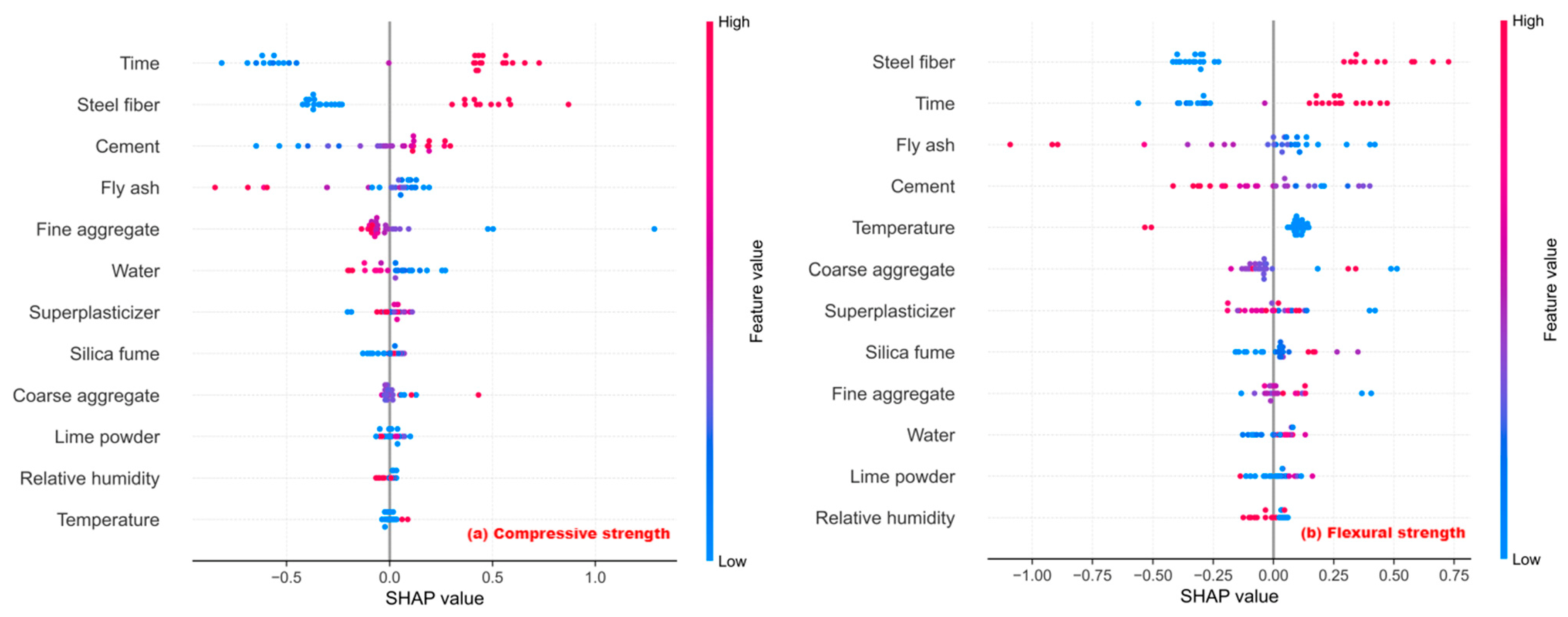
The SHAP summary analysis presented in Figure 13 illustrates significant disparities in the dominant factors across the four predictive targets, indicating that the effective information learned by the model evolves with the response variables. For compressive strength, the contributions are primarily driven by Time and Steel fiber, which exhibit the widest SHAP value spans and high directional consistency, identifying them as the most influential drivers of model output variability. In contrast, the contributions of Cement, Fly ash, and aggregate-related variables are more dispersed (Figure 13a), suggesting that their effects are characterized by stronger interval dependency and complex feature interactions. A similar sensitivity to Steel fiber and Time is observed for flexural strength (Figure 13b); however, the broader SHAP distributions for Fly ash and Cement indicate that they can either promote or inhibit the model output depending on the specific sample composition. 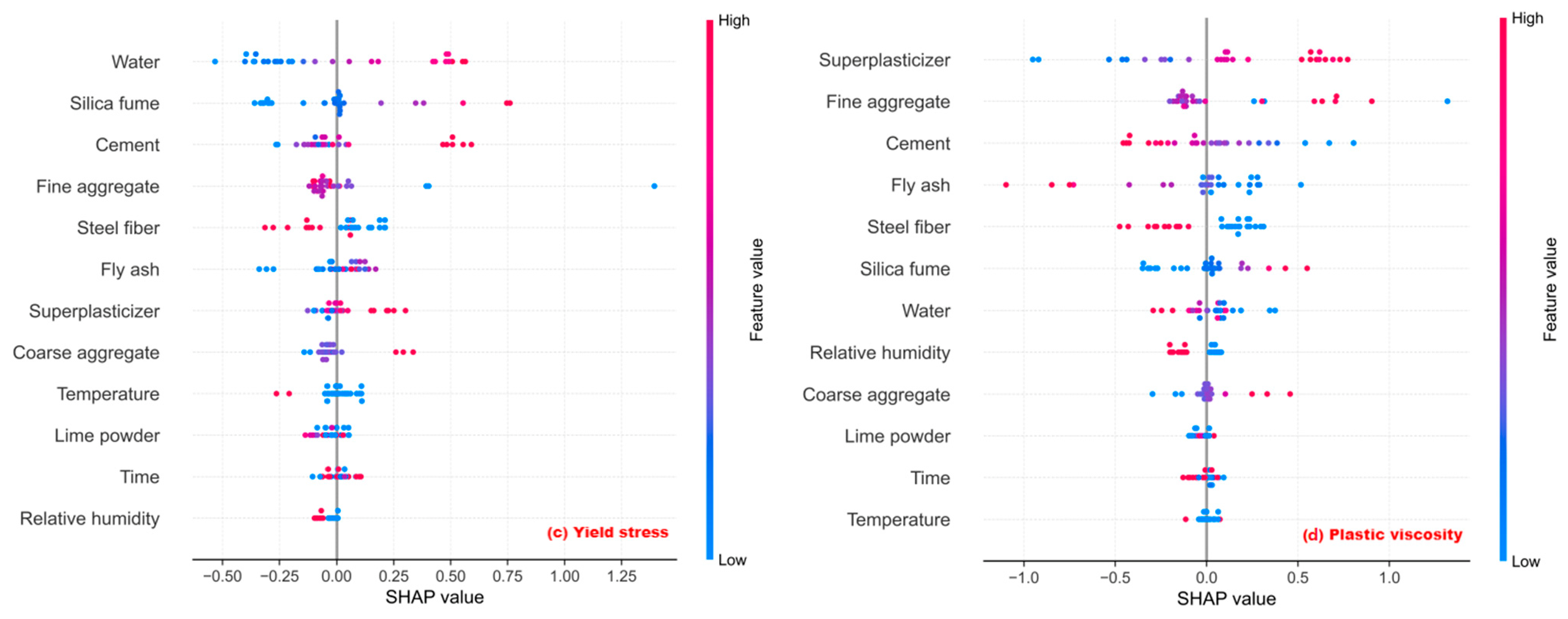Regarding yield stress (Figure 13c), the model shows higher sensitivity to paste-related parameters, with Water, Silica fume, and Cement occupying the most prominent positions, while the coexisting positive and negative contributions of certain variables (e.g., fibers and admixtures) reflect distinct sample dependency. Finally, plastic viscosity is predominantly driven by the Superplasticizer dosage, with a SHAP magnitude significantly exceeding other variables (Figure 13d). The SHAP distribution for viscosity exhibits a more pronounced heavy-tail characteristic, reflecting heightened complexity and uncertainty, which is consistent with the quantitative evaluation identifying viscosity prediction as the most challenging task.

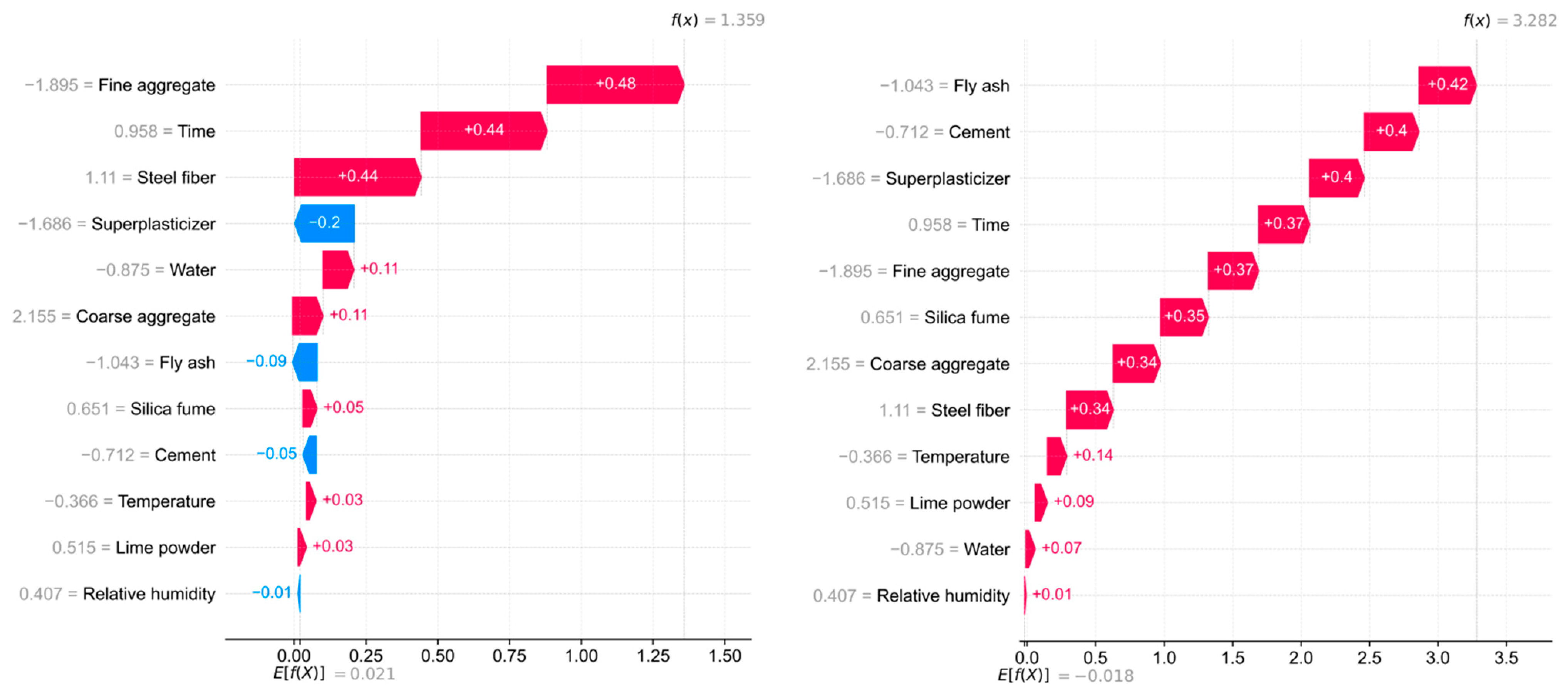
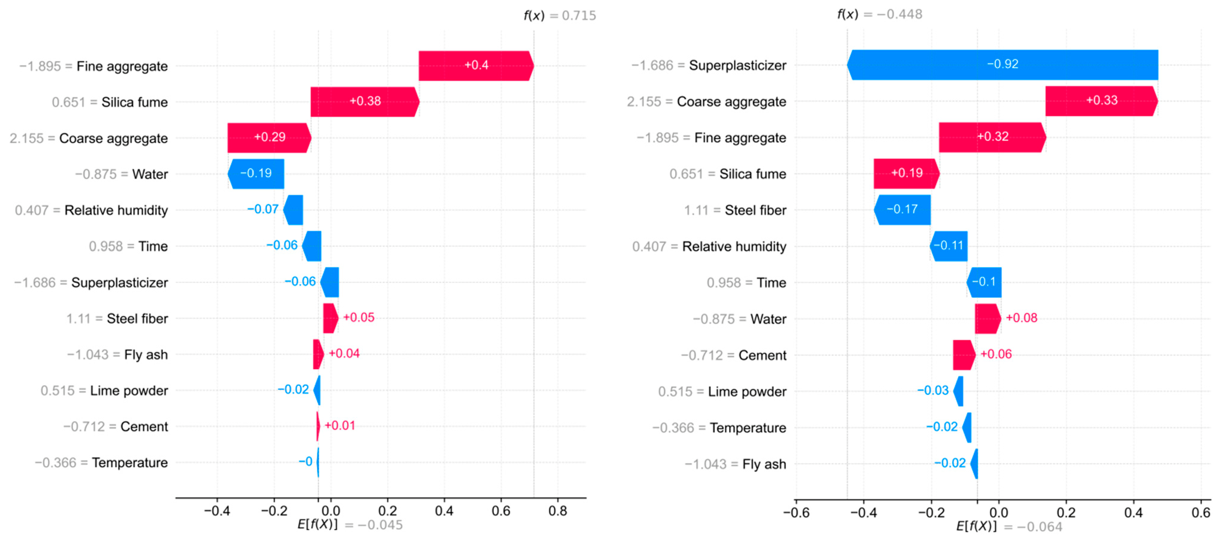
Using a test sample as an illustrative case, Figure 14 presents a waterfall decomposition that demonstrates how the final output f(x) is derived from the baseline E[f(x)] through the additive superposition of feature contributions. For compressive strength, the primary positive contributions originate from fine aggregate, time, and steel fiber, while superplasticizer and fly ash serve as the main negative contributors, collectively defining the net enhancement path for this specific instance. In the case of flexural strength, multiple variables, including fly ash, cement, superplasticizer, time, and aggregate-related features, exhibit additive positive contributions that synergistically drive the model output upward. For yield stress, fine aggregate, silica fume, and coarse aggregate act as the predominant positive terms, whereas water provides the most significant negative contribution, suggesting that moisture content exerts a strong inhibitory effect on the output for this sample. Finally, regarding plastic viscosity, the superplasticizer provides the most substantial negative contribution, dominating the final output direction; although aggregate and silica fume offer partial positive compensation, they remain insufficient to offset the net reduction induced by the chemical admixture.

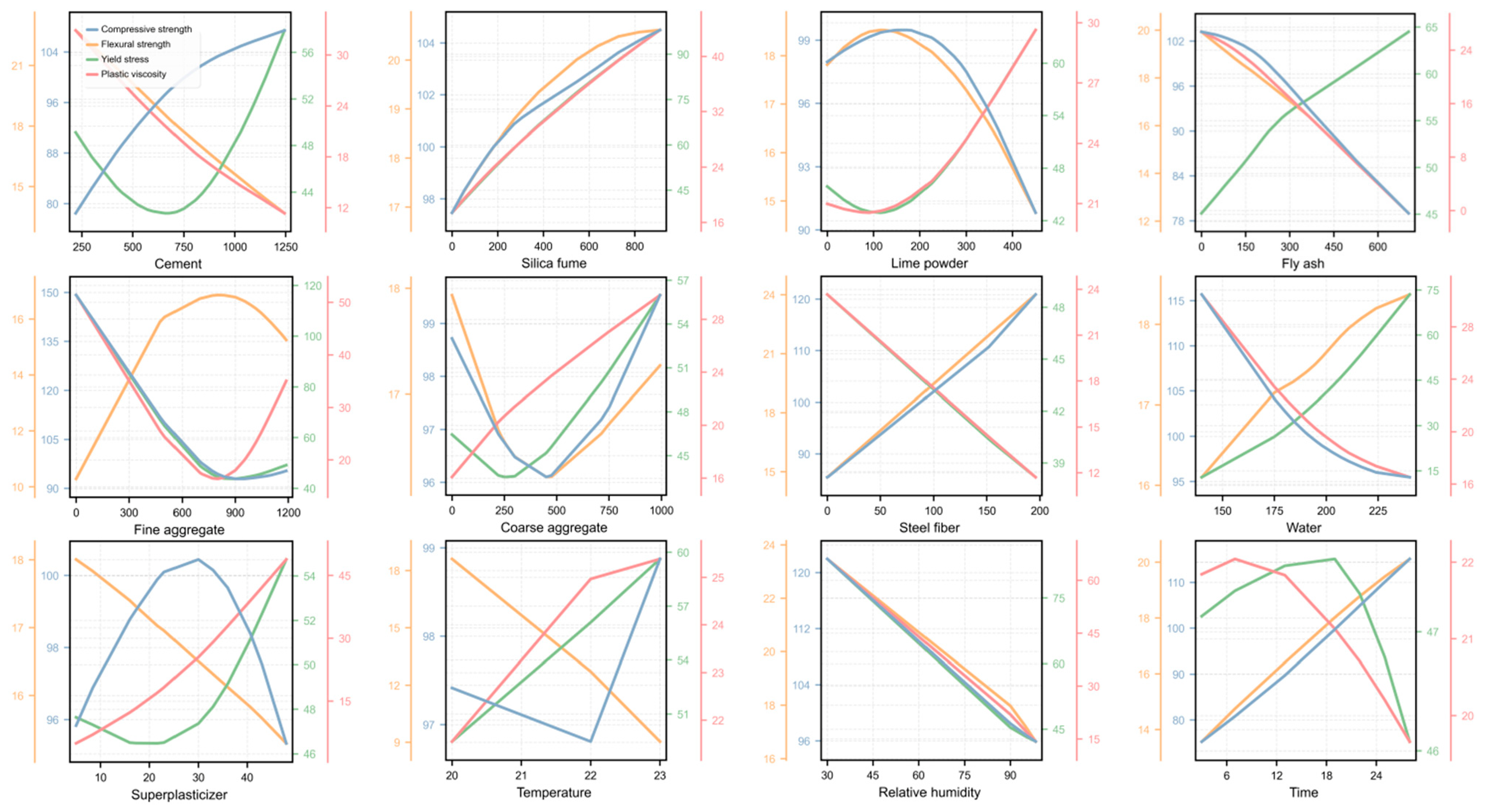
To complement the SHAP attribution results and visualize the average marginal response of model outputs to variations in input variables, Partial Dependence Plots (PDP) were further calculated and analyzed (Figure 15). By fixing a specific input feature while marginalizing over the remaining variables, PDP illustrates the overall influence of that feature on model predictions. In contrast to the aforementioned SHAP analysis, the PDP in this study employs the original output scales (non-standardized). Consequently, the curves in Figure 15 can be directly interpreted as the predicted response trends of each target in its respective physical units (MPa for strength, Pa for yield stress, and Pa·s for plastic viscosity).

Given the substantial differences in the dimensions and numerical ranges of the four targets, Figure 15 superimposes four PDP curves in each panel. Independent vertical axes, color-coded to their respective curves, are used to facilitate a comparison of the response morphologies across targets under the same input variable. Overall, the PDP reveals significant disparities in how targets respond to input variations, predominantly exhibiting nonlinear or interval-dependent characteristics. This suggests that the strength and rheological responses captured by the model are inconsistent in terms of their sensitive intervals and directional gradients.

Regarding binders and mineral admixtures (Cement, Silica fume, Fly ash, Lime powder), most target curves exhibit nonlinear curvature or varying marginal effects across different ranges. This indicates that these components do not contribute linearly to predictions; instead, they undergo response transitions or slope changes as the mix proportions evolve. The influence of admixtures and water-related variables (Superplasticizer, Water) is more pronounced for rheological outputs (yield stress and plastic viscosity), characterized by larger amplitudes and higher sensitivity. This implies that workability-related inputs exert a more direct driving force on rheological predictions, whereas their effects on strength-related outputs are more interval-dependent. Aggregate-related variables (Fine and Coarse aggregates) show distinct response directions or magnitudes across targets, underscoring the coupling between grading/content information and the strength–rheology nexus. Environmental and temporal factors (Temperature, Relative humidity, and Time) also exhibit target-dependent behavior; specifically, the sensitivity of strength outputs to Time is most significant, aligning with the global SHAP results regarding the importance of curing age.

It should be noted that the PDP describes the average marginal effect under the current data distribution and model assumptions. When input features are correlated, the marginalization process may be constrained by the data support domain. Therefore, interpretations of these curves in certain intervals should be conducted cautiously, considering the data coverage and simultaneous variations in other variables. Consequently, this study utilizes PDP as a supplement to SHAP: while SHAP identifies which variables drive changes in the output, PDP visualizes how the output responds to those changes, thereby providing global cross-validation of the model behavior.

4. Optimization: Ga-Based Mix Design

The optimization of UHPC mix proportions involves complex challenges, necessitating a comprehensive consideration of output targets, parameter constraints, and algorithmic settings. This study systematically establishes a model parameter system (see Algorithm 1). The model aims to design high-performance UHPC by evaluating four key performance indicators: compressive strength, flexural strength, yield stress, and plastic viscosity. The objective function $Y$ is constructed to identify the minimum value $Y_{\min }$ through iterative optimization.

Algorithm 1. GA-based UHPC Mix Proportion Optimization

Require: Population size N, max generations NGEN, crossover prob cxpb, mutation prob mutpb, elite count E, variance threshold ε, small constant δ; bounds L,U; constraints (Tmin,Tmax; w/b range; s/b range; performance thresholds); targets (fc*, ff*, τy*, μ*); weights (wc, wf,wτ,wμ); predictor model M(·).

Input: Candidate mix space defined by bounds and constraints; surrogate predictor M(·) trained for (fc, ff, τy, μ).

1. Initialize population P = {xi}{i=1…N} by sampling each gene xi[j] ~ Uniform(L[j], U[j]).

2. Evaluate fitness of each individual x in P using Fitness(x).

3. Set generation counter g = 1.

4. Evolution loop (g = 1 to NGEN):

While g ≤ NGEN do

a. Sort P by fitness F(x) in descending order and keep Elite = best E individuals.     b. Compute tournament probabilities pi = F(xi)/Σk F(xk).     c. Sample Parents with replacement from P using {pi} to form N − E parents.     d. Generate Offspring until |Offspring| = N − E:

i. Select two parents (p1, p2).       ii. If rand() < cxpb then perform single-point crossover at k ∈ {1, …, 9}; else copy parents.       iii. Apply Gaussian mutation to each gene with probability mutpb.       iv. Clip genes to bounds [L,U] (optional repair).       v. Add resulting children to Offspring.

e. Evaluate fitness for each x in Offspring using Fitness(x).     f. Form next generation: P ← Elite ∪ Best(Offspring, N − E).     g. If Var({F(x)|x ∈ P}) < ε then break (convergence).     h. g ← g + 1.

end while.

5. Extract FeasibleSet = {x ∈ P|Feasible(x) = true} and rank by minimal objective J(x).

6. Return top-3 feasible solutions (minimal J or maximal F).

Definitions: Feasible(x): returns true iff (i) L ≤ x ≤ U; (ii) Σx ∈ [Tmin,Tmax]; (iii) w/b and s/b within ranges; (iv) M(x) satisfies performance thresholds ($\widehat{{\mathrm{f}}_{\mathrm{c}}}$ ≥ fc,min, $\widehat{{\mathrm{f}}_{\mathrm{f}}}$ ≥ ff,min, $\widehat{{\mathsf{\tau }}_{\mathrm{y}}}$ ≤ τy,max, $\hat{\mathsf{\mu }}$ ≤ μmax). Objective J(x) = wc($\widehat{{\mathrm{f}}_{\mathrm{c}}}$ − fc*)2 + wf($\widehat{{\mathrm{f}}_{\mathrm{f}}}$ − ff*)2 + wτ($\widehat{{\mathsf{\tau }}_{\mathrm{y}}}$ − τy*)2 + wμ($\hat{\mathsf{\mu }}$ − μ*)2. Fitness F(x) = 1/(J(x) + δ) if Feasible(x) = true; otherwise set F(x) to a very small value.

Output: Top-3 feasible UHPC mix designs with improved prediction accuracy (minimal objective J).

The objective function $Y$ is defined in Equation (24), where ${\alpha }_1,{\alpha }_2,{\alpha }_3,{\alpha }_4$ are weighting coefficients. The individual target deviations are calculated as shown in Equation (25), where $f_{ct},f_{cp}$ represent the true and predicted compressive strengths, $f_{rt},f_{rp}$ are the flexural strengths, $Y{S}_t,Y{S}_p$ denote the yield stresses, and $P{V}_t,P{V}_p$ are the plastic viscosities.

$$Y={\alpha }_1{y}_1+{\alpha }_2{y}_2+{\alpha }_3{y}_3+{\alpha }_4{y}_4$$

(24)

$$y_1=|f_{ct}-f_{cp}|, y_2=|f_{rt}-f_{rp}|, y_3=|Y{S}_t-Y{S}_p|, y_4=|P{V}_t-P{V}_p|$$

(25)

Furthermore, constraints are applied to the dosages of each UHPC component based on data distributions and engineering requirements. As shown in

Table 7. Constraints for UHPC mixture optimization variables.

Mix Proportion	Cement	Silica Fume	Limestone Powder	Fly Ash	Fine Aggregate	Coarse Aggregate	Steel Fiber	Water	Superplasticizer
	kg/m3
Max	1200	400	200	300	1000	1000	200	400	200
Min	400	0	0	0	0	0	0	100	0

, the dosage ranges for nine input parameters are restricted. Additionally, the total dosage is constrained as per Equation (26) to meet practical engineering standards, where $D_i$ represents the dosage of each component:

$$2000\le D_C+D_{SF}+D_{LP}+D_{FA}+D_{sand}+D_{Gravel}+D_{Fi}+D_W+D_{SP}\le 2500$$

(26)

In the context of UHPC, the constraints on the water-binder (w/b) ratio are vital to model performance, as this parameter fundamentally defines the material’s low-porosity microstructure. Simultaneously, previous research has identified that the sand-binder ratio also exerts a significant influence on UHPC performance. Therefore, this section imposes constraints on both the w/b ratio (Equation (27)) and the sand-binder ratio (Equation (28)). To identify a mixed proportion that balances optimal mechanical properties and rheological characteristics, minimum thresholds are established for compressive and flexural strength, while maximum limits are set for yield stress and plastic viscosity. Considering the requirements for long-distance transportation and the enhancement of UHPC fluidity and pumpability, relatively low values for yield stress and plastic viscosity are preferred. These constraints are detailed in Equation (29).

$$0.15\le D_W/(D_C+D_{SF}+D_{LP}+D_{FA})\le 0.2$$

(27)

$$0.5\le (D_{sand}+D_{Gravel})/(D_C+D_{SF}+D_{LP}+D_{FA})\le 4$$

(28)

$$f_{cp}\ge 130,f_{rp}\ge 40,0<Y{S}_p\le 50,0<P{V}_p\le 50$$

(29)

To achieve the optimal mix design for UHPC, this study employs a Genetic Algorithm (GA). As a prominent class of evolutionary algorithms, the GA identifies optimal solutions by simulating natural processes such as selection, crossover, mutation, and adaptation. The hyperparameters and their respective value ranges for the GA used in this model are summarized in

Table 8. Model Hyperparameters.

Hyperparameter	Population Size	Generations	Crossover Probability	Mutation Probability	Tournament Size	Crossover Alpha	Mutation Gaussian
Symbol	population	NGEN	cxpb	mutpb	tournsize	alpha	mutGaussian
Value	100	100	0.5	0.2	3	0.5	0.2

. The algorithm assumes a population size $N$, where each individual $x_i(i=1,2,3,\dots ,N)$ represents a candidate solution. The population at iteration t can be represented as a matrix, as shown in Equation (30). The quality of each individual is evaluated by the fitness function f(x), as defined in Equation (31).

$$P(t)=\{x_1^t,x_2^t,\dots ,x_N^t\}$$

(30)

$$f:X\to R$$

(31)

In the selection operation, the probability of an individual $x_i$ being chosen is determined by its fitness value $f(x_i)$. For instance, using the roulette wheel selection strategy, the selection probability $p_i$ is calculated according to Equation (32), where $f_i$ is the fitness of individual $i$ and ${\displaystyle {\sum }_{j=1}^N{f}_j}$ is the total fitness of the entire population. The crossover operation simulates genetic recombination. Assuming a single-point crossover occurs at position $K$, the two newly generated offspring (Z₁, Z₂) are expressed as shown in Equation (33). The mutation operation enhances population diversity through random perturbations. For individuals using binary encoding, the mutation of a specific gene locus under a mutation probability $p_m$ is defined in Equation (34), where $r$ is a random number following a uniform (0, 1) distribution.

$$p_i={\displaystyle \frac{f_i}{{\displaystyle \sum _{j=1}^N{f}_j}}}$$

(32)

$$Z_1=(x_p[1:k],x_q[k+1:L]),Z_2=(x_q[1:k],x_p[k+1:L])$$

(33)

$$x_i[j]=\left\{\begin{array}{c}1-x_i[j], \mathrm{if} r<p_m\\ x_i[j],\mathrm{otherwise}\end{array}\right.$$

(34)

The new generation is a collection of new individuals produced through selection, crossover, and mutation. To improve convergence speed and the quality of solutions, an elitism strategy is typically adopted, where the individual with the highest fitness from the current population is directly preserved for the next generation, as shown in Equation (35). The algorithm terminates when the maximum number of iterations is reached or when the population fitness converges, i.e., the fitness variance falls below a threshold $\epsilon$, as expressed in Equation (36).

$$P(t+1)=Elite(P(t))\cup Offspring(P(t))$$

(35)

$$Var(f(x))<\epsilon$$

(36)

Through Genetic Algorithm (GA) optimization, three sets of candidate UHPC mix proportions were obtained (Samples 1–3,

Table 9. UHPC Mixture Optimization Output.

Input Parameter	Unit	Sample 1	Sample 2	Sample 3
Cement	Kg/m3	859.16	815.55	573.62
Silica Fume		167.71	82.5	307.30
Limestone Powder		131.93	21.35	143.40
Fly Ash		4.56	245.05	0.15
Fine Aggregate		156.90	650.87	500.78
Coarse Aggregate		795.50	485.33	751.17
Steel Fiber		25.256	132.05	152.20
Water		174.65	198.39	184.38
Superplasticizer		24.51	17.25	8.40

). To perform experimental validation, specimens were prepared according to these optimized proportions and tested for compressive strength, flexural strength, yield stress, and plastic viscosity. The predicted values were compared item-by-item with the experimental results (

Table 10. Error = Pred.–Exp.; positive values indicate overestimation.

Sample	Compressive Strength MPa			Flexural Strength MPa			Yield Stress Pa			Plastic Viscosity Pa·s
	Exp.	Pred.	Error	Exp.	Pred.	Error	Exp.	Pred.	Error	Exp.	Pred.	Error
Sample 1	139	145.11	6.11	52	56.84	4.84	25	20.59	−4.41	9	10.58	1.58
Sample 2	130	136.21	6.21	49	47.35	−1.65	30	21.34	−8.66	5	3.07	−1.93
Sample 3	133	125.06	−7.94	50	46.24	−3.76	48	45.76	−2.24	10	11.97	1.97

). To ensure comparability, specimen preparation and performance testing were conducted under standardized environmental conditions: T = 23–25 °C and RH = 90–95%. Across the three groups, the errors for compressive strength ranged from −4.94 to 6.21 MPa, and flexural strength errors ranged from −3.76 to 6.84 MPa. Regarding rheological properties, the yield stress error ranged from −9.41 to −4.24 Pa (exhibiting a slight overall underestimation), while the plastic viscosity error ranged from −1.93 to 1.97 Pa·s. Overall, the experimental results demonstrate strong consistency with the predictions, indicating that the GA-driven mix design is technically feasible and can effectively support the “Optimization—Experiment—Validation” development workflow for mix proportions.

5. Conclusions

This study developed an integrated data-driven framework for the multi-property prediction and inverse mix design of UHPC by combining cross-source data harmonization, VAE-based augmentation, multi-output deep learning, interpretability analysis, and GA-driven optimization. A dataset containing 139 valid UHPC records with four synchronized target properties was curated from 22 peer-reviewed studies and expanded to 2780 samples, providing improved data support for small-sample modeling.

The proposed multi-output DNN achieved robust predictive performance for the joint estimation of compressive strength, flexural strength, yield stress, and plastic viscosity, with test-set R² values of 0.8601, 0.9212, 0.8464, and 0.6603, respectively. Comparative benchmarking showed that the proposed model delivered the most balanced overall performance across the four targets, while ablation analysis confirmed that VAE-based augmentation was a key contributor to the observed gains in accuracy and generalization under small-sample conditions.

Interpretability analysis further showed that the dominant drivers varied across target properties. Curing age and steel fiber content were most influential for strength-related responses, whereas water-to-binder ratio and superplasticizer dosage played more prominent roles in rheological behavior. These findings indicate that the model captured physically meaningful feature–response relationships rather than merely fitting statistical correlations.

Finally, coupling the trained surrogate model with a GA enabled the generation of candidate UHPC mixtures, and experimental validation of three optimized samples showed good agreement between predicted and measured values. Overall, this work provides a transparent and engineering-oriented pathway for integrated UHPC prediction, interpretation, and optimization, while also highlighting that rheological targets, especially plastic viscosity, remain the most challenging and should be prioritized in future data expansion and model refinement.