Article

Surrogate-Based Resilience Assessment of SMRF Buildings Under Sequential Earthquake–Flood Hazards


School of Computing, Engineering and Digital Technologies, Teesside University, Middlesbrough TS1 3BX, UK
*
Author to whom correspondence should be addressed.
Buildings 2026, 16(1), 48; https://doi.org/10.3390/buildings16010048
Submission received: 5 September 2025 / Revised: 30 September 2025 / Accepted: 15 December 2025 / Published: 22 December 2025

Abstract

This study presents a framework for assessing the resilience of steel special moment-resisting frame (SMRF) buildings under sequential earthquake–flood hazards. Surrogate models, including a stacked attention-based LSTM network (Stack-AttenLSTM) and CatBoost, are developed to predict key engineering demand parameters (EDPs), particularly maximum inter-storey drift ratios (MIDRs), avoiding the need for computationally expensive nonlinear time history analysis (NLTHA). The predicted EDPs are integrated with the FEMA P-58 methodology to estimate repair costs and durations, while the REDi framework is used to capture recovery delays and functionality loss. A two-storey code-compliant SMRF building is evaluated under a design-basis earthquake (DBE) with and without a subsequent 4.0 m flood. Results show that the combined hazard nearly doubles repair costs (from 0.33 to 0.77 of replacement value), increases downtime from 194 to over 411 days, and reduces the resilience index (Ri) from 0.873 to 0.265. These findings highlight the severe impacts of cascading multi-hazard events and the need to extend performance-based design toward resilience-focused strategies. The proposed surrogate-based framework provides a practical tool for evaluating multi-hazard risks and guiding the design of more resilient structures.

1. Introduction

Recent disasters, especially earthquakes and floods, have underscored the significant vulnerability of communities to natural hazards. In 2023 alone, floods and earthquakes resulted in damages amounting to $20.37 billion and $17.62 billion, respectively [1,2]. To mitigate such risks, engineers are actively developing strategies aimed at reducing the impacts of future hazards and bolstering the resilience of individuals and their assets. A notable advancement has been the transition from a code-based design philosophy to a performance-based design approach, which aims to align the anticipated performance of structures with the expected consequences of hazards [3]. The objective is to set clear goals so that structures can endure an acceptable level of damage under defined hazard intensities [4]. For instance, the Federal Emergency Management Agency (FEMA) has introduced a methodology for probabilistic estimation of economic losses in buildings subjected to earthquakes, referred to as FEMA P-58 [5]. This framework encompasses four primary steps: (i) estimating seismic hazard through ground-motion intensities or hazard curves; (ii) evaluating structural response using nonlinear analysis; (iii) representing the structural response in terms of drifts and accelerations; (iv) estimating damage to both structural and non-structural elements, as well as contents, through fragility functions.
FEMA P-58 offers a probabilistic framework for assessing building performance concerning repair costs, downtime, and casualty risks across various seismic hazard intensities. Recently, this methodology has gained traction for evaluating, comparing, and enhancing the seismic performance of diverse structural systems. For instance, Jarrett et al. [6] employed the FEMA P-58 framework to contrast innovative and traditional seismic resisting systems, illustrating its effectiveness in quantifying the impact of design decisions on repair costs and downtimes. Guerrero et al. [7] demonstrated that the integration of buckling-restrained braces (BRBs) in hospital buildings situated on extremely soft soil can result in substantial economic advantages, as measured by the FEMA P-58 methodology, by mitigating seismic damage and losses. Likewise, Liu et al. [8] conducted FEMA P-58 evaluations on various configurations of eccentrically braced steel frames, revealing that the brace configuration significantly affects collapse probabilities and loss outcomes, with K-braced frames showing enhanced collapse resistance and reduced expected losses compared to other types. These investigations underscore the importance of advanced loss assessment in informing design optimisations aimed at enhancing seismic resilience.
In addition to innovations in structural systems, researchers have explored various elements that influence seismic losses and recovery, as evaluated by the FEMA P-58 framework. For example, Ghods and Rofooei [9] quantified economic losses and repair durations for various occupancy types, highlighting the necessity of customising seismic design to align with regional hazard characteristics. This is exemplified in a case study conducted in Semnan, Iran, where site-specific hazards and soil conditions played a crucial role in shaping the design spectrum and anticipated performance. Furthermore, Safiey et al. [10] discovered that prolonged earthquakes can considerably enhance damage accumulation and financial losses in contemporary steel moment frames, even when peak intensities remain comparable. These findings emphasise that hazard characteristics extending beyond peak intensity, such as duration and frequency content, can significantly affect building performance. Indeed, Ramírez et al. [11] combined the Pacific Earthquake Engineering Research (PEER) Performance-Based Earthquake Engineering methodology with FEMA P-58 to assess economic seismic performance, elucidating how intensity measures (IMs) translate through engineering demand parameters (EDPs) and damage states to decision variables like repair costs and downtime. Their research highlights the critical need to connect hazard analysis with consequence modelling to facilitate comprehensive performance evaluations.
Recent advancements have been made in downtime and functional recovery modelling. The REDi (Resilience-based Earthquake Design Initiative) rating system, created by Almufti and Willford [12], offers guidelines for estimating repair time by taking into account not just physical repairs but also hindrances such as inspections, financing, permitting, and delays in mobilisation. By dividing downtime into phases and suggesting improved design and planning strategies, the REDi framework sets clear resilience objectives (for instance, restoring functionality within a specified number of days). Similarly, Terzic et al. [13] introduced a modelling framework aimed at predicting the functional recovery trajectory of buildings post-earthquake, considering damage and repair limitations. Gallegos et al. [14] illustrated the practical application of these methodologies by evaluating both loss and downtime in reinforced concrete (RC) wall-frame office buildings, contrasting various design strategies regarding their seismic resilience performance. Their research quantified how specific design improvements (such as additional damping or structural fuses) could lead to reductions in repair times and economic losses, thus enhancing overall resilience. In a similar context, Takaya et al. [15] assessed the financial implications of different beam-to-column connection types in steel office buildings through FEMA P-58 analysis, revealing that the detailing of connections has a significant impact on damage and repair cost distributions. Collectively, these studies underscore a transition in earthquake engineering research towards not only preventing structural collapse but also reducing economic repercussions and downtime.

2. Research Motivation

Despite advancements in the application of the FEMA P-58 framework in structural engineering, many studies continue to focus on single-hazard scenarios, particularly earthquakes considered in isolation. Nevertheless, structures in specific areas may face sequential or compound hazards, such as a significant earthquake followed by flooding (resulting from levee failures, tsunamis, or intense rainfall in a compromised watershed). These multi-hazard occurrences can lead to severely compounded impacts on buildings. The earthquake may cause structural impairment and weaken various components, after which the flood exerts additional stress on an already damaged structure, frequently resulting in destruction that far exceeds the impact of either hazard independently. Recent scholarly work on multi-hazard risk remains relatively limited; a review conducted by the authors revealed the absence of prior surrogate modelling tools capable of swiftly predicting structural responses and resilience levels under combined earthquake–flood loading [16]. To assess the multi-hazard resilience of structures, conventional analyses must be conducted (for example, considering combined flood and seismic events or sequences of hurricanes). These methodologies often depend on comprehensive simulations. Consequently, the FEMA P-58 framework has yet to be extended to assess the resilience of buildings in such multi-hazard contexts.
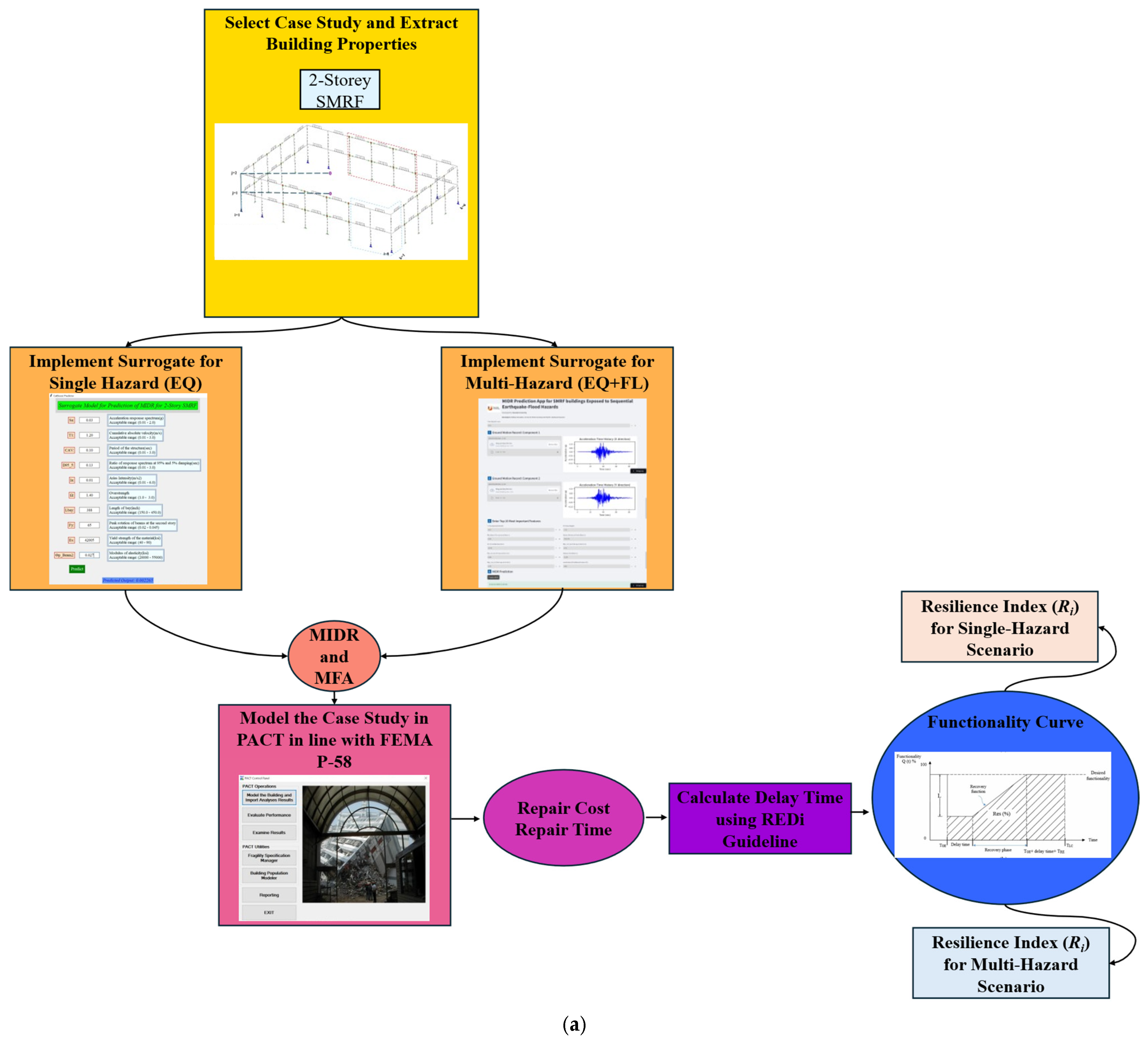
This paper seeks to establish and illustrate a surrogate-based resilience assessment for steel special moment-resisting frame (SMRF) buildings subjected to a sequential earthquake–flood scenario. By utilising data-driven surrogate models, the computational difficulties associated with simulating numerous intricate multi-hazard events are effectively tackled, facilitating the efficient estimation of critical EDPs for loss and downtime evaluations. The methodology integrates surrogate-predicted seismic and flood demands with the FEMA P-58 loss assessment and REDi recovery framework to derive a quantitative resilience index (Ri). The present study extends existing surrogate models into a complete resilience assessment framework by coupling them with FEMA P-58 for loss estimation and REDi for downtime modelling. This constitutes the first application of surrogate-based hazard–response predictions to quantify Ri under cascading earthquake–flood hazards. This framework is applied to a 2-storey code-compliant SMRF building as a case study, contrasting its performance in an earthquake-only scenario against that of an earthquake followed by significant flooding, defined here as a rapid inundation with a 4.0 m water depth that fully submerges the first storey and imposes combined hydrostatic and hydrodynamic loads on the damaged structure. While the case study focuses on a low-rise structure, the same framework can also be applied to mid- and high-rise SMRF buildings, provided that surrogate models are specifically developed and trained for those building types. Figure 1a illustrates the comprehensive workflow employed in this research. The process initiates with the selection of a representative case study, specifically the 2-storey SMRF building. The essential input parameters necessary for the surrogate models are identified and compiled. In the subsequent phase, the surrogate models created for the earthquake-only scenario, as well as for the earthquake followed by flood scenario, are utilised to produce EDPs, with a specific emphasis on maximum inter-storey drift ratio (MIDR) and maximum floor acceleration (MFA), since these two parameters are the primary drivers of damage in the FEMA P-58 framework [5]. MIDR strongly governs drift-sensitive components such as structural frames, partitions, and façades, while MFA predominantly affects acceleration-sensitive non-structural systems such as suspended ceilings, equipment, and mechanical installations.
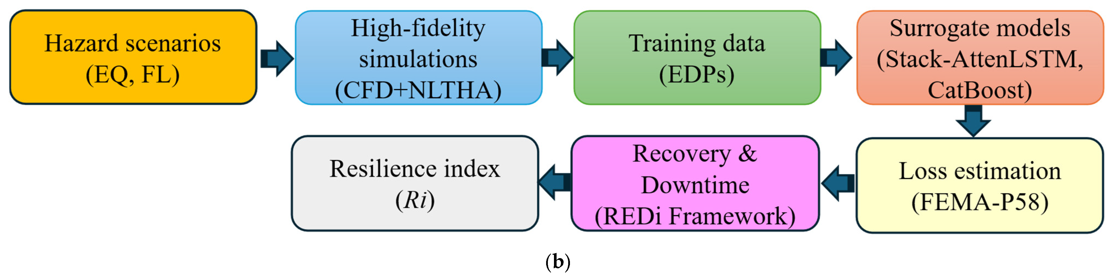
Subsequently, the Performance Assessment Calculation Tool (PACT) [17] developed by FEMA under the FEMA P-58 guidelines is utilised to estimate the costs and durations of building repairs resulting from both single- and multi-hazard scenarios. A critical aspect of evaluating resilience is estimating the delay time before recovery efforts can begin. To incorporate this, the methodology outlined in the REDi guideline is employed. By utilising the results from the preceding steps, which include repair time, repair cost, and delay time, the functionality curve for the SMRF building is created. Ultimately, resilience indices are calculated for both hazard scenarios. The ensuing comparison sheds light on how the incorporation of a flooding event can impact the seismic resilience of SMRF buildings, thereby highlighting the significance of accounting for multi-hazard interactions in resilience evaluations. Also, Figure 1b shows the streamlined workflow for resilience assessment of SMRF buildings, where high-fidelity simulations generate training data for surrogate models (Stack-AttenLSTM and CatBoost), which efficiently predict EDPs. These predictions feed into FEMA P-58 for loss estimation, the REDi framework for recovery analysis, and ultimately the calculation of the Ri. The highlighted surrogate modelling stage represents the central methodological contribution of this study.

3. Methodology

3.1. Structural Model and Hazard Scenario

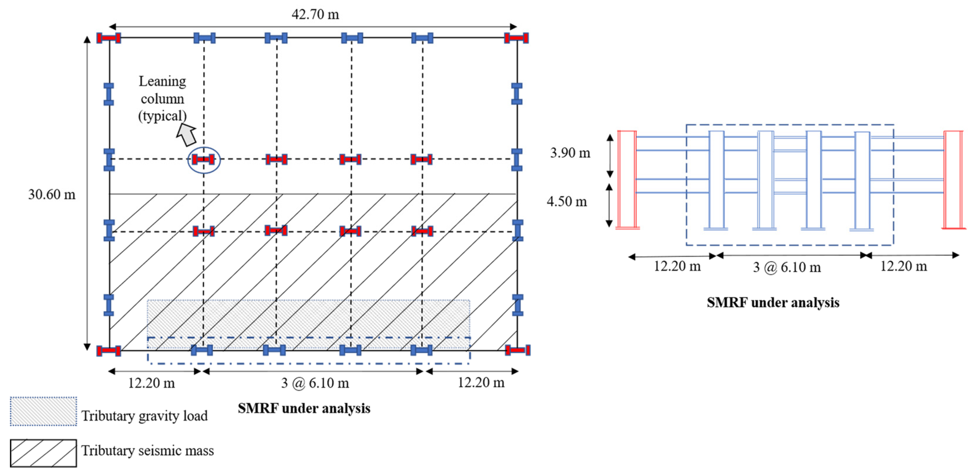
The case study building is a 2-storey SMRF designed according to modern U.S. seismic provisions. The structure features reduced beam section (RBS) beam-to-column connections, which are commonly used to improve ductility and energy dissipation capacity in SMRFs [18]. The building’s lateral system consists of perimeter SMRF bays, detailed per FEMA P695 [19] and AISC 341-05 [20] requirements to sustain ductile yielding in beam-ends while preventing column failure. It is representative of a low-rise building, with an initial fundamental period T1 = 0.91 s and storey heights of 4.5 m (first storey) and 3.9 m (second storey). Gravity loads include 4.8 kN/m2 dead load and 2.4 kN/m2 live load on the floors. The structure is assumed to be located in Los Angeles, California, on firm soil (Site Class D), with design spectra corresponding to Seismic Design Category Dmax as per ASCE 7-05 [21]. The beam and column sizes for the building are detailed in Table 1, while Figure 2 provides elevation and plan views of the building. Additional building characteristics and design details are available in [22].
Two hazard scenarios are examined: (1) Earthquake-only (EQ), which refers to a seismic event that aligns with the 10%/50-year design basis earthquake (DBE) intensity specific to Los Angeles; and (2) Earthquake + Flood (EQ + FL), where the same earthquake is immediately succeeded by a significant flood with an inundation depth of 4.0 m. The earthquake input is characterised by a spectrum-compatible ground motion that reflects DBE shaking. The flood hazard is envisioned as a sudden inundation (for instance, resulting from intense precipitation or levee failure) that occurs shortly after the earthquake, causing the building to endure both hydrodynamic and hydrostatic loading while it remains in a compromised state [23]. To effectively represent this sequential loading, Samadian et al. [23] established a comprehensive framework for assessing the multi-hazard vulnerability of buildings subjected to earthquakes and floods. This framework divides the structural response analysis into two distinct phases: initially, the earthquake ground motion is applied, and once the seismic activity ceases, the building (which may exhibit residual deformations and damage) is then subjected to the flood loading. A free-vibration interval is incorporated between the two hazards to accommodate any transient oscillations that may dissipate. In their research, the flood is modelled as a rapidly ascending inundation that envelops the first storey up to 4 m, generating hydrostatic pressure on walls and buoyancy forces, in addition to hydrodynamic drag forces acting on structural components due to water flow. Subsequently, these loads are allocated along the submerged sections of the columns and walls, utilising pressure profiles derived from computational fluid dynamics simulations (OpenFOAM) for a 4 m inundation with the flow velocity taken into account [23]. By applying the flood loads to the earthquake-damaged structure without resetting the damage, the analysis effectively captures the cumulative damage impact of the multi-hazard scenario [23].

3.2. Damage Assessment Using the FEMA P58 Framework

The FEMA P-58 methodology, developed under the ATC-58 project in partnership with FEMA, represents a significant advancement in performance-based seismic assessment. Unlike conventional prescriptive design, it adopts a probabilistic and consequence-oriented approach that addresses the needs of engineers, building owners, insurers, and policymakers. Its development occurred in two phases:
Phase 1: Creation of a comprehensive methodology for seismic performance assessment.
Phase 2: Development of performance-based seismic design guidelines.
A core tool of this framework is the PACT, which integrates component fragility data and consequence functions to model building responses under earthquake loading. Key features of FEMA P-58 and PACT include:
Performance metrics assessed: repair costs, repair times, casualties, environmental impacts, and energy use.
Component modelling:
  • Both structural and non-structural components are grouped into Performance Groups (PGs).
  • Each component is defined by fragility functions linking EDPs, such as MIDR and MFA, to specific Damage States (DSs).
  • Damage is represented as discrete states with associated consequences, rather than as continuous scales.
  • Damage correlation (correlated vs. uncorrelated) can be specified within each PG.
Consequence modelling:
  • Once DSs are identified, consequence functions translate them into repair costs and repair durations.
  • Costs are based on standardised construction cost models (2011 Northern California baseline), adjusted for inflation and regional variations.
  • Repair times account for labour productivity and sequencing strategies (serial vs. parallel repairs).
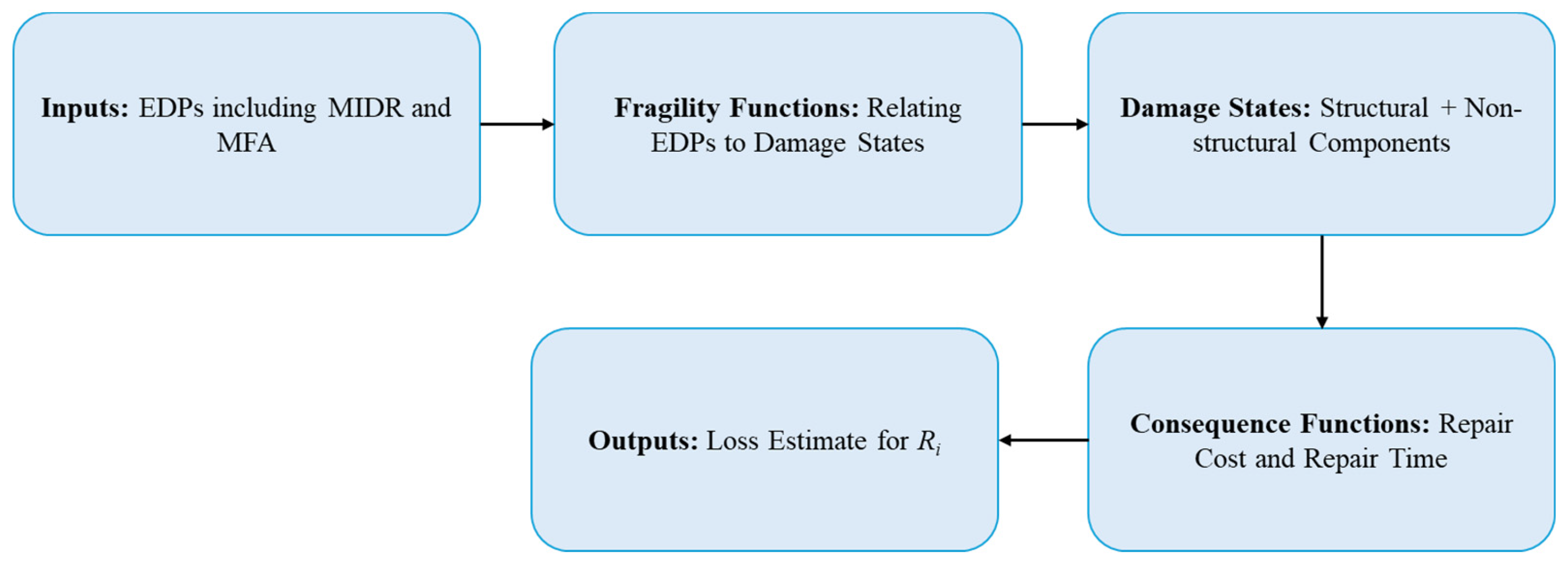
To aid comprehension, a schematic flowchart (Figure 3) is provided to illustrate the key steps of the FEMA P-58 damage assessment process as applied in this study. The procedure begins with the input of EDPs, specifically the MIDR and MFA, which are obtained from surrogate models. These EDPs are then passed through fragility functions defined in PACT, which relate structural and non-structural components to their probability of reaching various damage states. Once the potential damage states are identified, consequence functions are applied to translate these states into quantifiable outcomes such as repair costs and repair times. These consequences are then synthesised to generate the outputs, namely probabilistic loss estimates and recovery metrics, which serve as the basis for calculating the Ri.
In this research, the FEMA P-58 methodology is implemented through PACT to evaluate both seismic and multi-hazard resilience of the case study two-storey SMRF building. PACT outputs, repair costs and repair times for structural and non-structural PGs, are integrated into the Ri calculation. Finally, FEMA P-58 provides three assessment types:
Intensity-based: evaluates performance at a defined ground motion intensity.
Scenario-based: examines building response to a specific earthquake event.
Time-based: analyses building performance over its service life, accounting for the probabilistic occurrence of multiple events.
By linking physical damage with economic and functional consequences, FEMA P-58 enhances the reliability of resilience assessments and informs more effective seismic design and retrofit strategies.

3.3. Resilience Index (Ri)

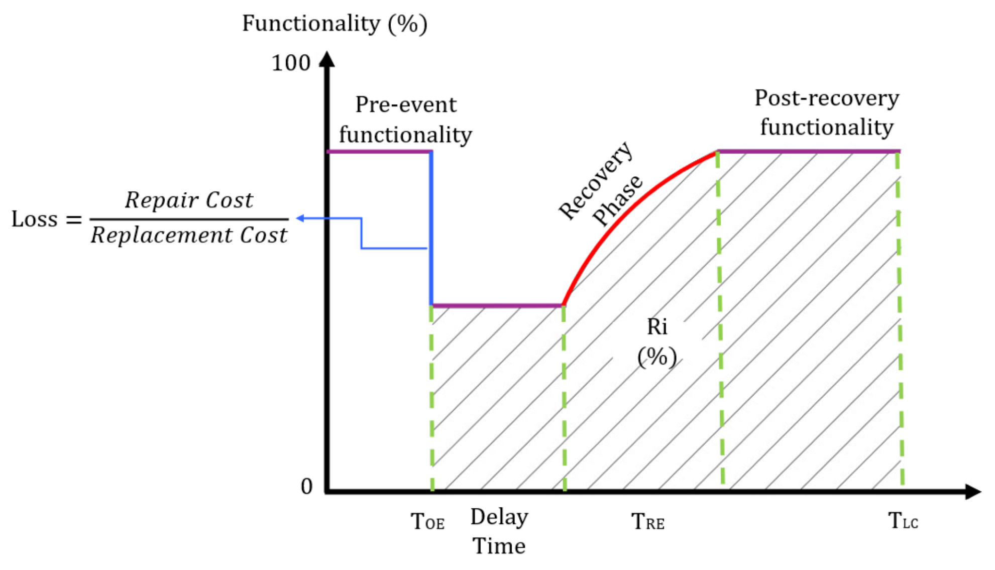
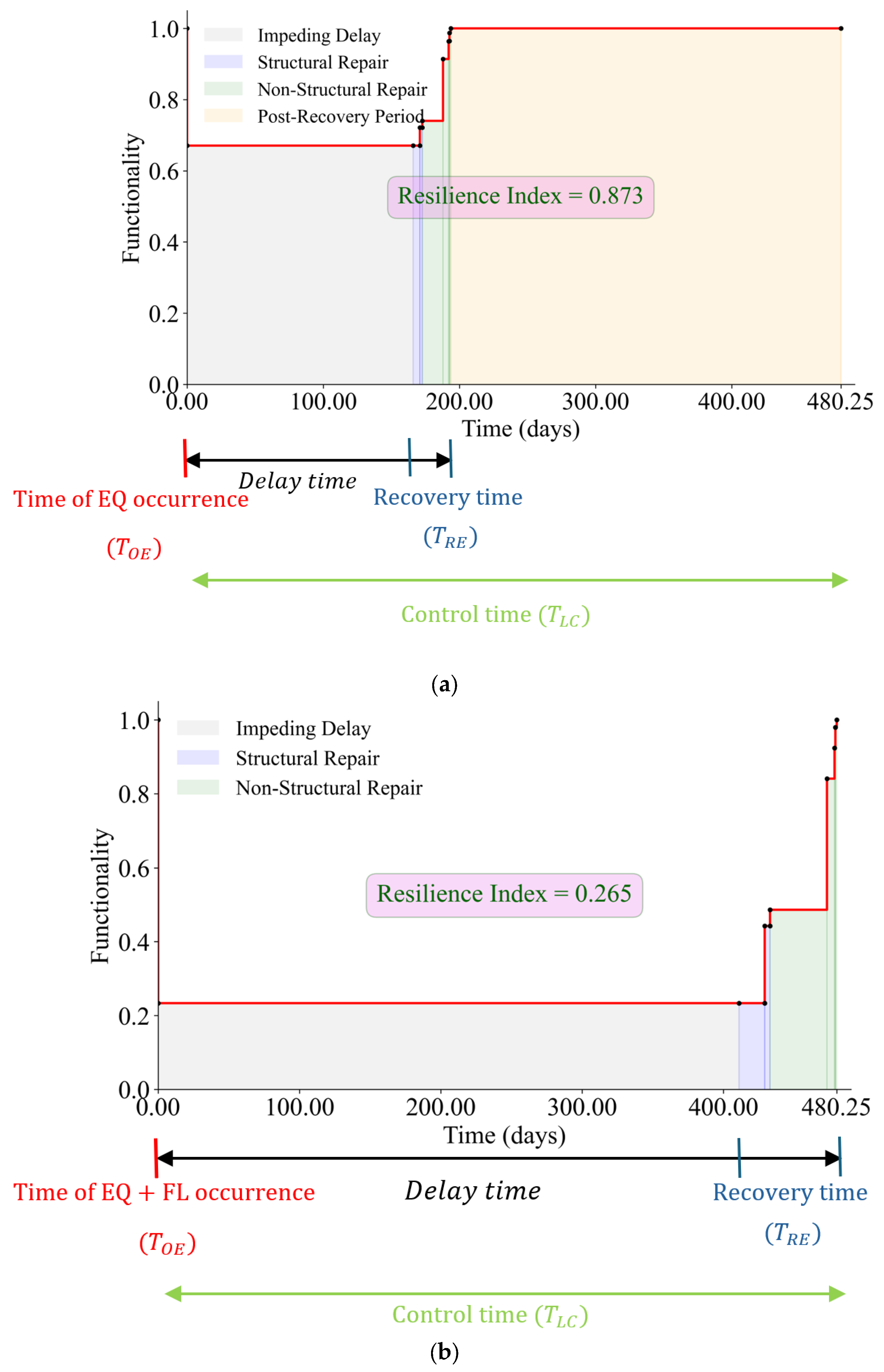
Resilience, within the realms of structural engineering and disaster risk management, denotes the capacity of a building or system to maintain its functionality and restore its performance after experiencing a disruptive event [24]. This notion is often depicted through a functionality curve, which demonstrates the progression of a building’s performance over time, starting from its initial state before the event, through the damage and recovery phases, to its ultimate condition post-recovery. Ri is quantitatively defined as the area beneath this functionality curve across a designated time frame, commonly known as the control time (TLC), and is represented as a percentage [25]. As illustrated in Figure 4, the functionality curve initiates with the building functioning at full capacity prior to any disruption. At a specific point in time, referred to as TOE, an external event such as an earthquake or flood transpires, resulting in a rapid decrease in functionality. The extent of this loss is indicative of the damage incurred, frequently measured as the ratio of repair expenses to the total replacement cost of the building. After the disruptive event, the building does not instantly transition into a recovery phase. There exists a time lag, termed delay time, before restoration efforts begin. This delay may arise from a variety of factors, including logistical issues, permitting holdups, interrupted utilities, resource limitations, and constraints in labour allocation.
Once the recovery process commences, the building progressively restores its functionality over a duration referred to as recovery time, TRE. The rate and degree of this recovery are influenced by the extent of the damage, the effectiveness of the reconstruction efforts, and the level of financial investment. Based on these variables, the building may ultimately be returned to its original pre-event state, or to a condition characterised by either diminished or improved performance. The recovery path, illustrated by the slope and configuration of the functionality curve, is thus essential for comprehending the resilience of a structure. The control time, indicated as TLC, specifies the maximum duration during which resilience is assessed. This period is established according to the significance of the structure and the expectations of stakeholders or policymakers. For example, critical infrastructure such as hospitals or emergency services may be mandated to restore functionality within a significantly shorter timeframe than non-essential buildings. Ri is subsequently computed as the area beneath the functionality curve from TOE to TLC, normalised by the total area that signifies complete functionality throughout that interval.
In this research, the resilience of a two-storey SMRF building is assessed under two distinct hazard scenarios: the DBE event with a return period of 500 years (EQ only scenario), and a combined hazard scenario that includes a DBE followed by a flood with a water depth of 4 m (EQ + FL = 4 m scenario). For each scenario, data regarding repair costs and repair times are sourced from the PACT, following the FEMA P-58 methodology. Furthermore, the delay time prior to the commencement of recovery is estimated utilising the REDi framework. Repair cost, repair time, and delay time are employed to develop the functionality curves for both hazard scenarios. The resulting resilience indices offer a comparative assessment of the impact of flooding on the seismic resilience of the SMRF building, thereby highlighting the importance of incorporating multi-hazard considerations in contemporary resilience evaluations.

3.4. Surrogate Modelling of Structural Response

To apply the FEMA P-58 framework for loss estimation, it is crucial to first assess the EDPs. This generally necessitates the execution of NLTHA to derive the MIDR and MFA for the building in question. Nevertheless, conducting high-fidelity NLTHA over a broad spectrum of possible earthquake–flood sequences can be computationally intensive. Therefore, this research utilises surrogate models to efficiently estimate the structural response (EDPs). In a previous study [22] by the authors, a database of nonlinear simulation outcomes was created for thousands of randomised SMRF configurations subjected to earthquake loads, which served as a basis for training surrogate models for the single-hazard scenario. Conversely, for the sequential hazard analysis, the authors established an integrated 3D simulation framework (OpenSeesPy in conjunction with OpenFOAM) to generate a training dataset of dynamic responses of the 2-storey SMRF under combined earthquake and flood loading [23]. The input parameters for this multi-hazard dataset encompass characteristics of the earthquake ground motion (such as time histories of acceleration) and flood parameters (including inundation depth), along with the structural attributes of the building. The output responses captured from the simulations include MIDR and MFA during the earthquake, followed by the flood. These EDPs are selected as they serve as critical indicators of damage for both structural and non-structural components in accordance with FEMA P-58.

3.4.1. Single-Hazard Surrogate Model

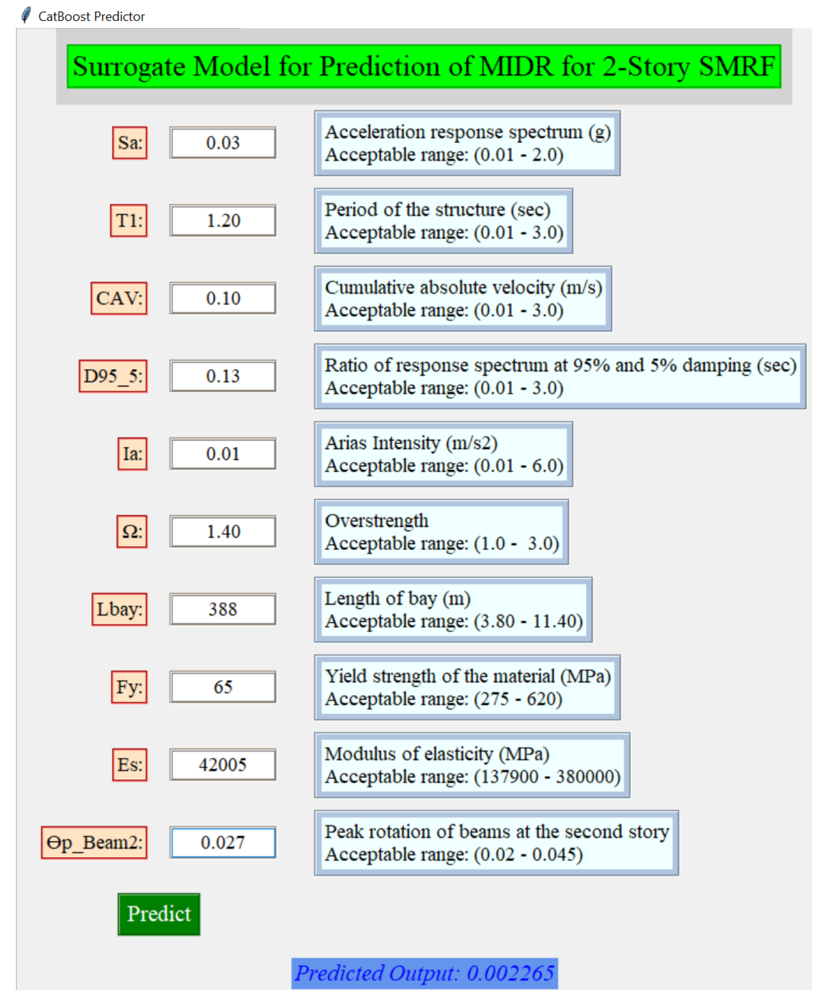
In the scenario focused solely on earthquakes, a surrogate model created by the authors [22] was employed to forecast the peak MIDR and MFA of the two-storey SMRF building based on ground motion IMs. Initial investigations evaluated a variety of machine learning (ML) algorithms, including random forests, gradient boosting, neural networks, linear regression, and support vector machines, utilising a comprehensive meta-database of simulated building responses [22]. The final model chosen for the single-hazard scenario was a CatBoost model, which demonstrated exceptional accuracy in predicting peak drifts and accelerations across the spectrum of ground motions considered. This model effectively captures the nonlinear seismic response characteristics, accounting for the influences of spectral shape and magnitude through features such as spectral acceleration at the first-mode period (Sa(T1)), significant duration (D95-5), cumulative absolute velocity (CAV), and Aris intensity (Ia). Additional input parameters for the surrogate model include the fundamental period of the structure (T1), overstrength factor (Ω), bay length (Lbay), yield strength of steel (Fy), modulus of elasticity (Es), and peak rotation of beams at the second storey level ( θ p B e a m 2 ). The surrogate model is capable of predicting MIDR without the necessity of conducting a nonlinear time history analysis (NLTHA) for each new input. Readers are encouraged to refer to reference [22] for further details regarding these input parameters and the training and validation process of the CatBoost model for predicting the seismic response of SMRF buildings.
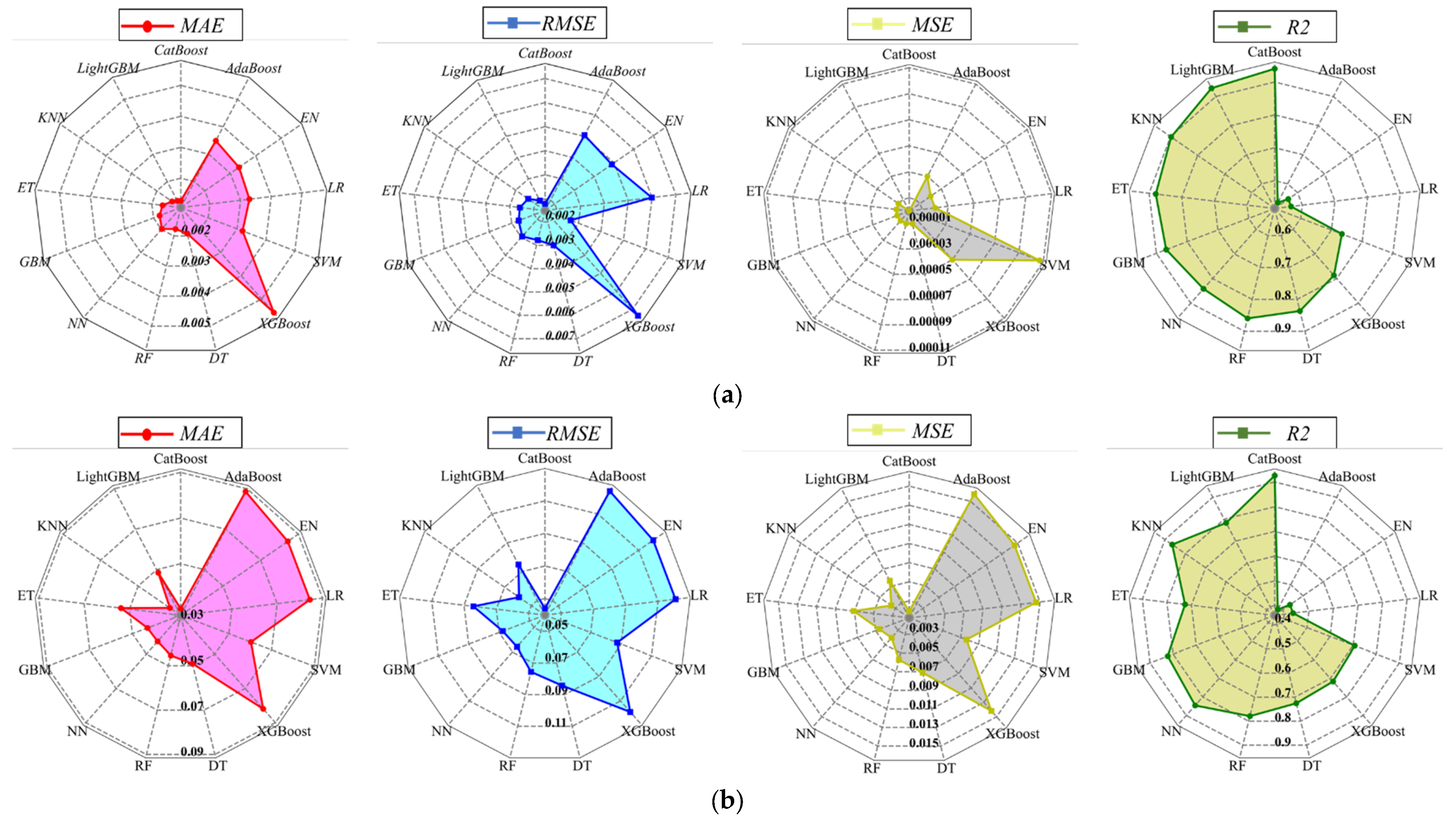
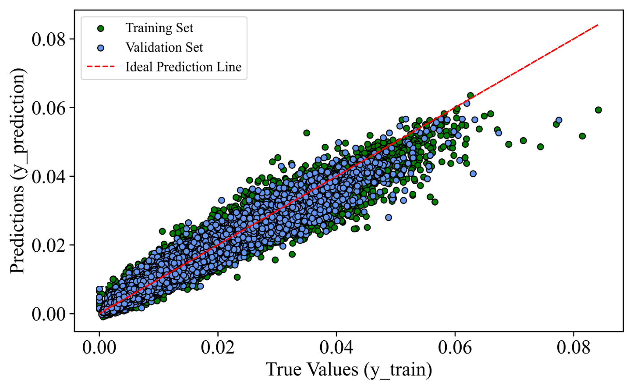
The surrogate model was trained on a meta-database of 30,000 SMRF building configurations generated via OpenSeesPy. Probabilistic variation in geometry, material properties, and hysteretic parameters ensured realistic design coverage. The primary EDPs of interest were MIDR and MFA, both exhibiting lognormal-type distributions. The dataset was randomly split into 80% training and 20% testing, and five-fold cross-validation was employed. To benchmark performance, 13 different ML algorithms were tested (Figure 5). Among these, CatBoost consistently demonstrated the best predictive capability, achieving R2 = 0.94 for MIDR and R2 = 0.92 for MFA, with mean absolute error (MAE) < 0.002 for MIDR and low root mean square error (RMSE) values. Scatter plots (Figure 6) further confirm the close alignment between predicted and true values on unseen test sets, underscoring CatBoost’s strong generalisation ability. This evidence supports the choice of CatBoost as the final EQ-only surrogate model for MIDR and MFA prediction. Figure 7 illustrates the graphical user interface (GUI) developed for the surrogate model aimed at predicting MIDR resulting from earthquake loads on the two-storey SMRF.

3.4.2. Multi-Hazard Surrogate Model

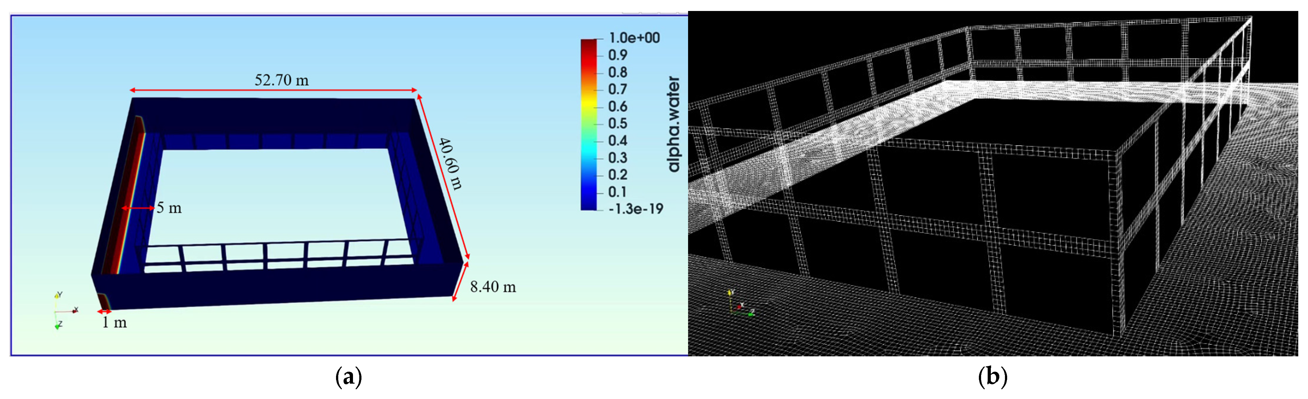
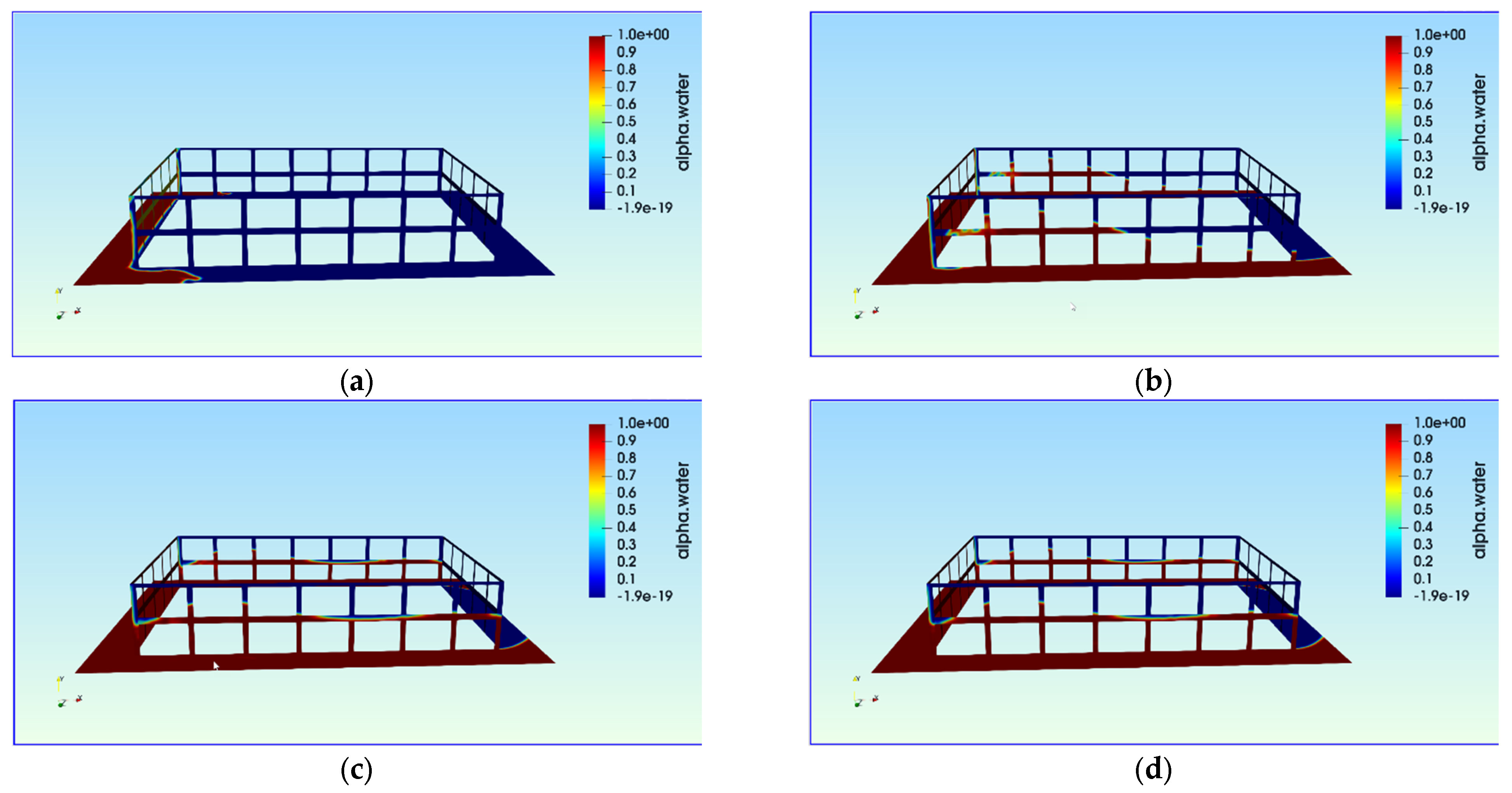
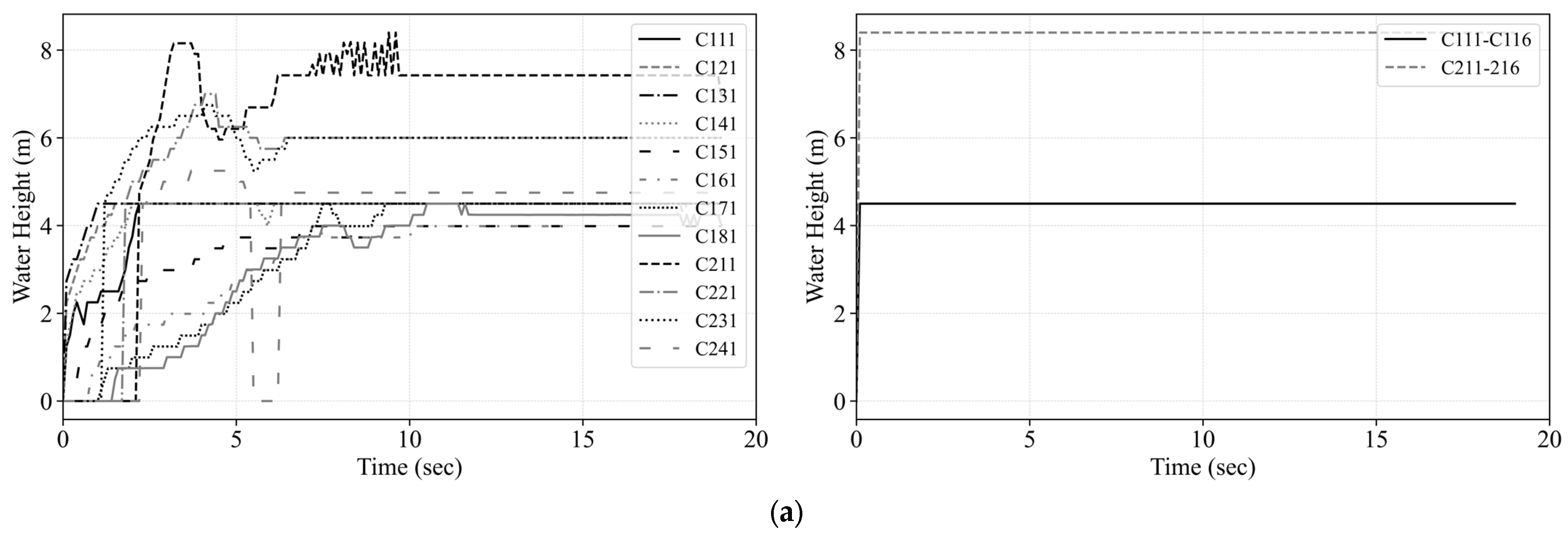
In the more intricate earthquake–flood scenario, a data-driven surrogate model was developed using a Stacked Attention Long Short-Term Memory (Stack-AttenLSTM) neural network [26]. This architecture combines the temporal learning capacity of LSTM cells with an attention mechanism that highlights the most critical segments of the seismic input, enabling improved capture of nonlinear, time-dependent structural responses under sequential hazards. The training dataset was generated from high-fidelity NLTHA and computational fluid dynamics (CFD)-informed flood simulations of three-dimensional (3D) SMRF buildings, developed in OpenSeesPy and OpenFOAM. Appendix A presents the detailed CFD analysis, including the CFD setup (Figure A1 and Table A1) and the resulting hydrodynamic loads (Figure A2 and Figure A3). A large meta-database of 30,000 SMRF structures was employed, with probabilistic variation in geometry, material properties, and hysteretic parameters to ensure broad coverage of low-, mid-, and high-rise configurations. From this, representative samples were selected via clustering methods to capture the full variability in dynamic properties. Ground motion records were chosen for a wide range of hazard levels, while flood scenarios were defined at depths of 0.30, 1.0, 2.0, and 4.0 m to represent increasing levels of severity [26].
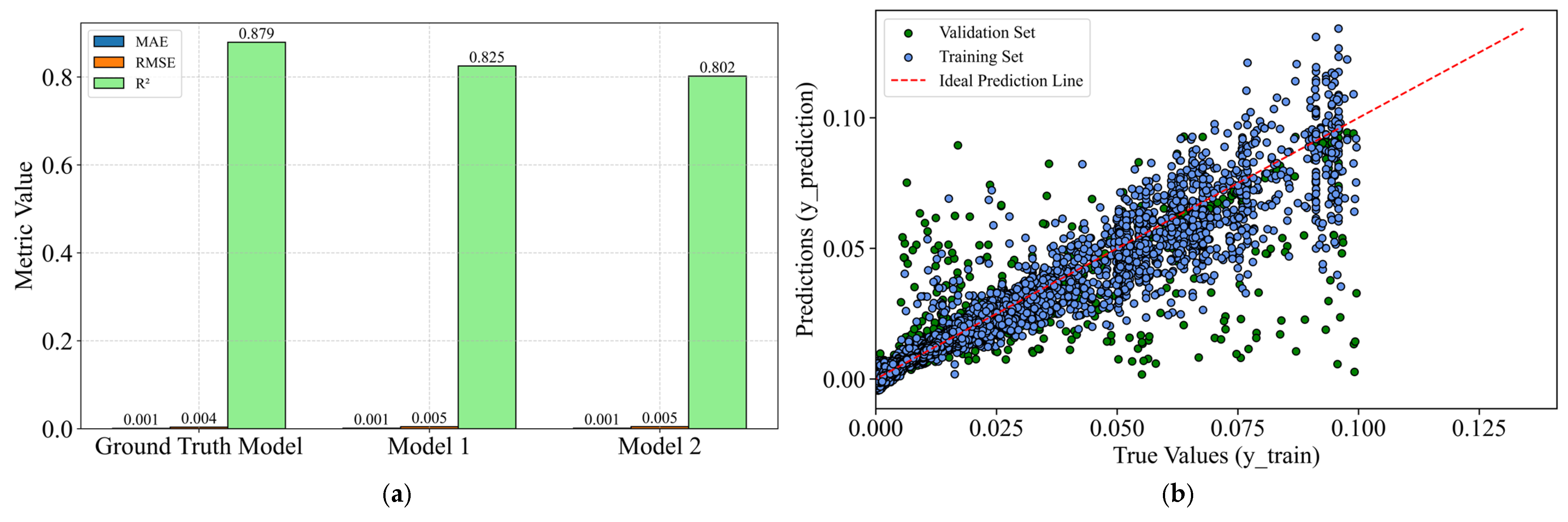
The surrogate model integrates both time-series inputs (two-component acceleration records segmented into stacks) and static features (structural geometry, material strengths, modal properties, and flood intensity). This hybrid input representation enhances generalisation and ensures sensitivity to both dynamic loading and building-specific characteristics. The surrogate model was trained on a coupled dataset generated by integrating OpenSeesPy seismic simulations with OpenFOAM hydrodynamic flood analyses. Four flood depths (0.30, 1.0, 2.0, 4.0 m) were considered, applied to probabilistically varied SMRF structures consistent with the EQ-only database. MIDR and MFA again served as the EDPs. Statistical analyses confirmed right-skewed output distributions, with both mean and variance increasing with flood depth. The dataset was partitioned into 80% training and 20% testing, and cross-validation was used to control overfitting. Several LSTM-based architectures were benchmarked, with the proposed Stack-AttenLSTM emerging as the most robust (Figure 8).
The ground-truth Stack-AttenLSTM achieved R2 = 0.879, RMSE = 0.004, and MAE = 0.001 across three random seeds, outperforming baseline LSTM variants (Figure 8a). The parity plot demonstrates a tight clustering of predicted vs. true MIDR values, confirming reliable generalisation to unseen multi-hazard scenarios (Figure 8b). These results validate the model’s capacity to capture the nonlinear, coupled effects of earthquake and flood loading, enabling reliable resilience assessments without resorting to computationally intensive full-order simulations.
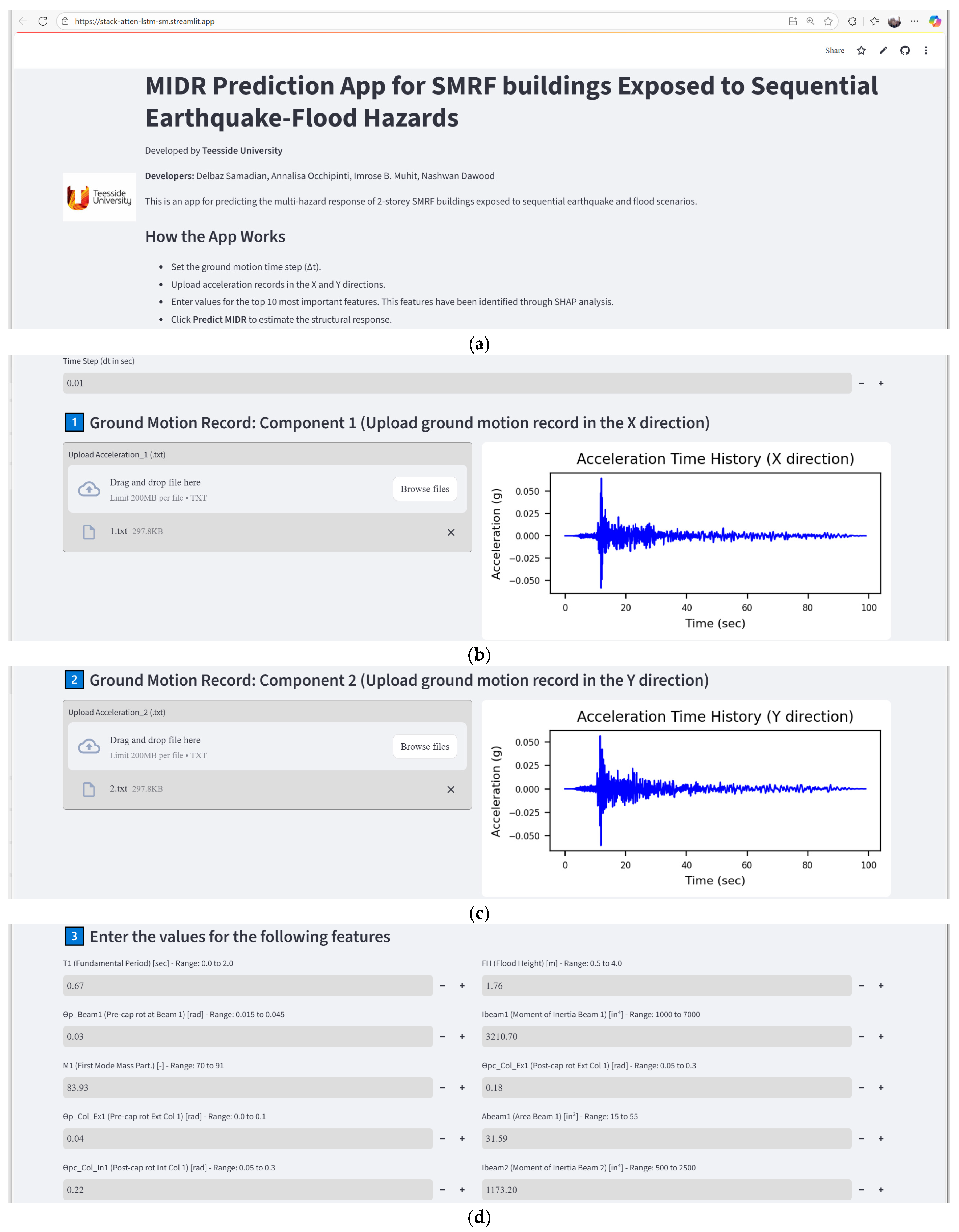
For demonstration purposes, a simple graphical interface was developed to enable users to query the trained model, as illustrated in Figure 9. As depicted in Figure 9, the application developed [26] for this study offers a step-by-step interface, from file upload to MIDR prediction, along with clear user instructions. The application processes ground motion time history data in both horizontal directions of X and Y from user-uploaded text files, as demonstrated in Figure 9b,c. Users have the ability to define the time step (dt) parameter for both ground motion records. The application visualises the time histories of these records, offering users immediate visual feedback. As illustrated in Figure 9d, users subsequently input values for the ten features. The application processes the time series and normalises the features prior to inputting them into the trained Stack-AttenLSTM model. Ultimately, the model forecasts the MIDR, and the results are interactively presented on the web interface, as depicted in Figure 9e. Additional information regarding the architecture and validation of the surrogate model is available in the authors’ previous work [26].
It should be noted that only MIDR and MFA were employed as EDPs in the surrogate models. This choice aligns with the FEMA P-58 methodology, which defines fragilities and consequences for both structural and non-structural components in terms of drift- and acceleration-sensitive responses. In the sequential earthquake–flood framework adopted here, it is assumed that non-structural elements such as infill walls are severely damaged or fail during the earthquake phase [23]. Consequently, the residual flood demands are resisted primarily by structural components (beams, columns, and connections), and their effects are sufficiently represented by MIDR and MFA. Flood-specific deterioration mechanisms (e.g., corrosion or water-soaked finishes) are typically associated with long-term inundation and are therefore beyond the scope of this study. Future extensions of the framework could expand the FEMA P-58 fragility library or incorporate additional non-structural elements to explicitly capture such effects.

3.5. Extract EDPs from Surrogate Models

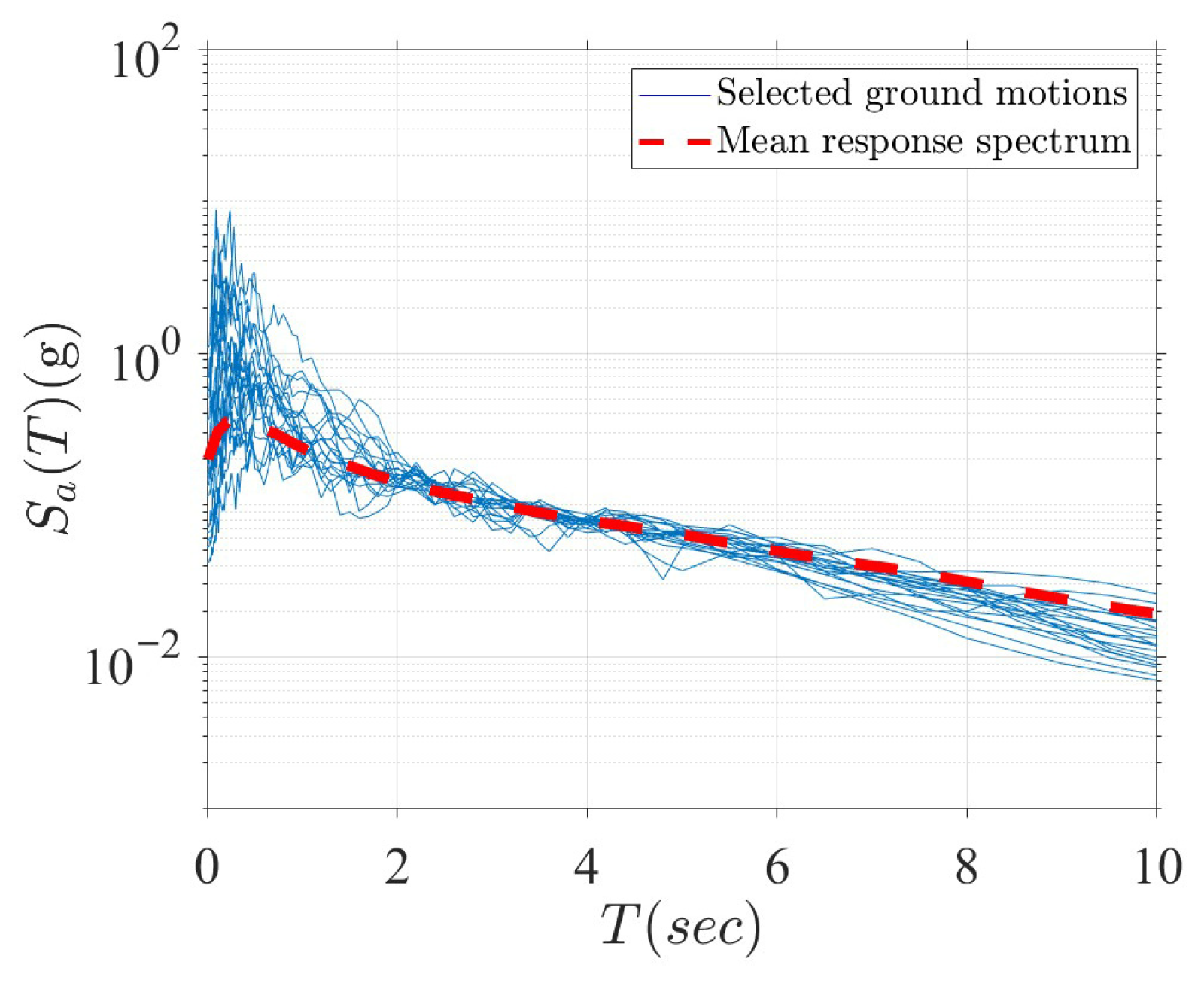
Before modelling the two-storey SMRF building in the PACT, it is crucial to extract the EDPs that correspond to the hazard levels being considered. As previously mentioned, Ri is assessed for two scenarios: EQ only and EQ + FL = 4 m. The aim is to evaluate the effect of flooding on the building by analysing its influence on Ri. To acquire the necessary EDPs for these hazard scenarios, the surrogate models outlined in Section 3.4.1 and Section 3.4.2 are utilised. For the characterisation of seismic demand, a selection of ground motion records is required. In this study, 20 ground motion records associated with a return period of 500 years are chosen from the NGA-West 2 database [27], which contains approximately 7000 mainshock records from 277 earthquakes. The method proposed by Samadian et al. [28] is employed for spectrum matching and scaling, wherein they introduced a modified conditional mean spectrum (CMS). This method is based on a previous probabilistic seismic hazard analysis (PSHA) performed for California, from which the uniform hazard curves (UHCs) were derived. These UHCs provide the basis for constructing the CMS at various hazard levels. The CMS process initiates by calculating the hazard curve using PSHA for a designated conditioning period (T), which acts as the reference period for defining spectral acceleration demand, S a ( T ) . The methodology also integrates weighted factors across different time intervals to ensure that the selected ground motions more accurately represent the target hazard spectrum at each intensity level [28]. Figure 10 illustrates the selected ground motion records for the two-storey SMRF building. These ground motions are utilised as input for both surrogate models to extract MIDR and MFA values for the reference two-storey SMRF building. The distinction in the surrogate model lies in the fact that, for the surrogate utilised in the EQ-only scenario outlined in Section 3.4.1, parameters such as Sa(T1), D95−5, CAV, and Ia are derived from each ground motion record. In contrast, for the surrogate employed in the EQ + FL scenario detailed in Section 3.4.2, the time history of acceleration is utilised.
Using the extracted MIDR values via surrogate models, fragility curves can be developed to estimate the conditional probability of exceeding specified performance limit states. In this study, these fragility functions are derived using the coefficient-based method proposed by Su and Lee [29], which assumes that the structural demand parameter D follows a lognormal distribution. This implies that D is related to a normally distributed variable X by L n D = X . Typically, the demand D is expressed as a power function of the IM, as given in Equation (1):
D = a ( I M ) b
where a and b are regression coefficients determined through a coefficient-based method.
X = L n D = L n a + b   L n I M
The mean ( m x ) and standard deviation of X, σ x , can be estimated as:
m x ( I M ) = L n ( a ( I M ) b )
σ x = σ L n ( D ) = 1 n 2 i = 1 n L n ( δ i a   I M i b ) 2
here, δ i are the observed demand values. The probability of exceeding a damage threshold C, given a certain intensity measure, is then expressed as:
P f = P ( D > C I M )   =   1     Φ ( L n C     m x ( I M ) σ x )
where Φ is the standard normal cumulative distribution function.
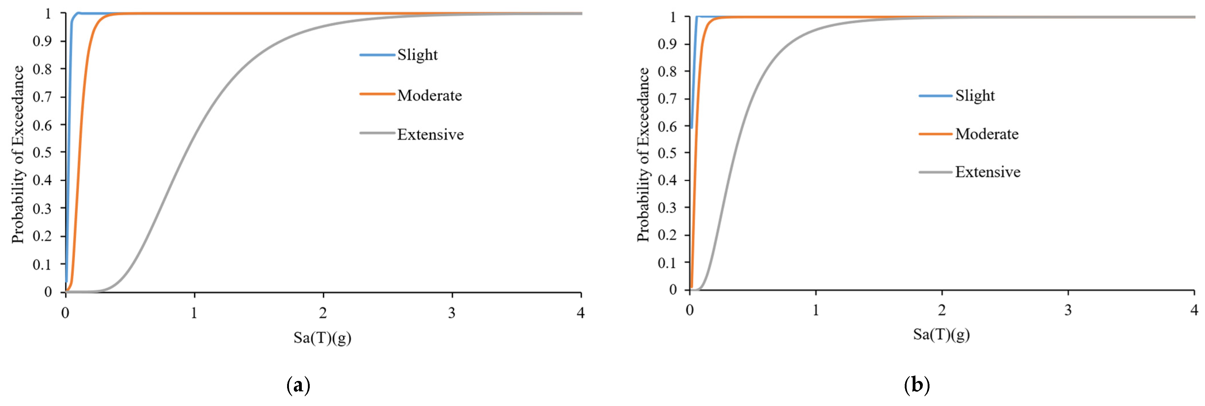
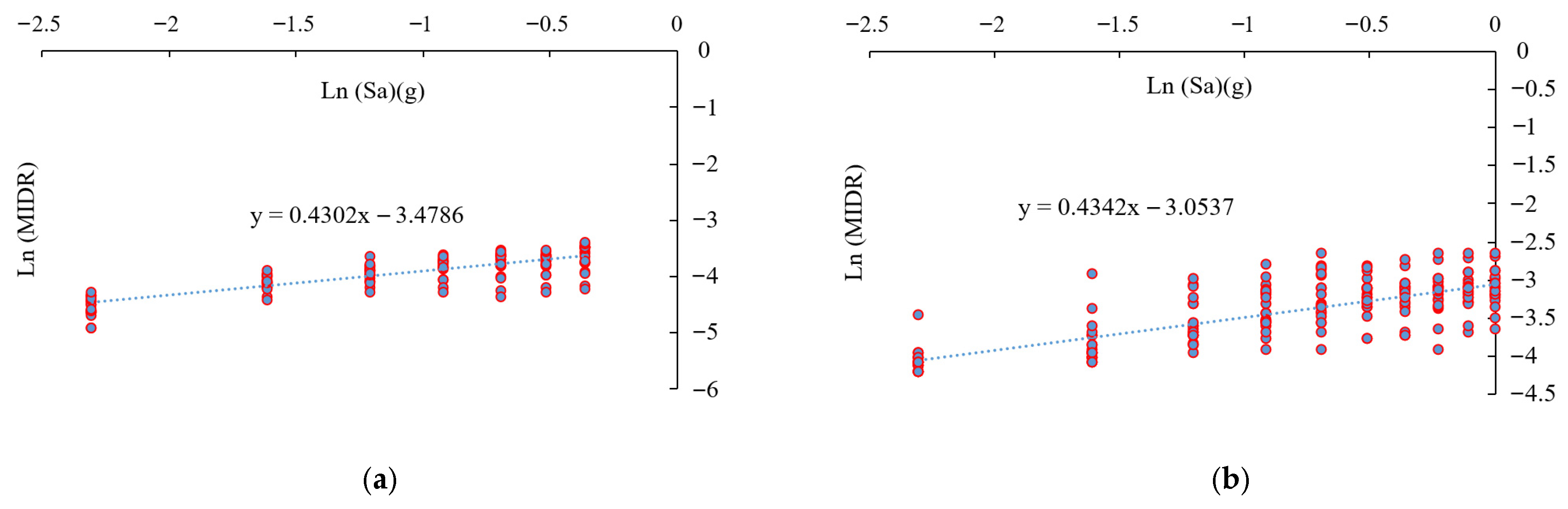
Figure 11 displays the outcomes of the regression analysis performed on MIDR values derived from the surrogate models for both the EQ only and EQ + FL = 4 m at the DBE hazard level. Additionally, Figure 12 depicts the resulting fragility curves for three damage states, slight, moderate, and extensive, for both the single-hazard (earthquake-only) and multi-hazard (earthquake followed by flood) scenarios, obtained through the methodology proposed by Su and Lee [29]. The comparison clearly shows that flooding significantly increases the fragility of the two-storey SMRF building across all damage states. For example, under the multi-hazard scenario, the probability of exceeding a given damage state at the same intensity measure level is consistently higher than in the earthquake-only case. This shift is primarily due to the compounded effects of hydrodynamic loads applied to an already seismically damaged structure, which accelerates stiffness and strength degradation in the lower storey columns and beams. The capacity thresholds C for the three damage states are sourced from Table 5.19 of the HAZUS-MH-MR 6 guideline [30], with values set at 0.006 for slight damage, 0.012 for moderate damage, and 0.03 for extensive damage. Since the surrogate models were specifically developed based on drift values related to non-collapse performance, the complete damage state is omitted from the analysis. This fragility-based evaluation therefore not only highlights the impact of sequential hazards but also serves as a crucial initial step for estimating loss and functionality parameters in the subsequent phases of the resilience assessment.

3.6. Inputs to PACT

After extracting the necessary EDPs, the PACT is employed to model the 2-storey SMRF building for seismic and multi-hazard loss assessment. This process begins with the definition of general building characteristics. Table 2 summarises the key building data input to PACT (e.g., floor area, structural system, replacement cost).
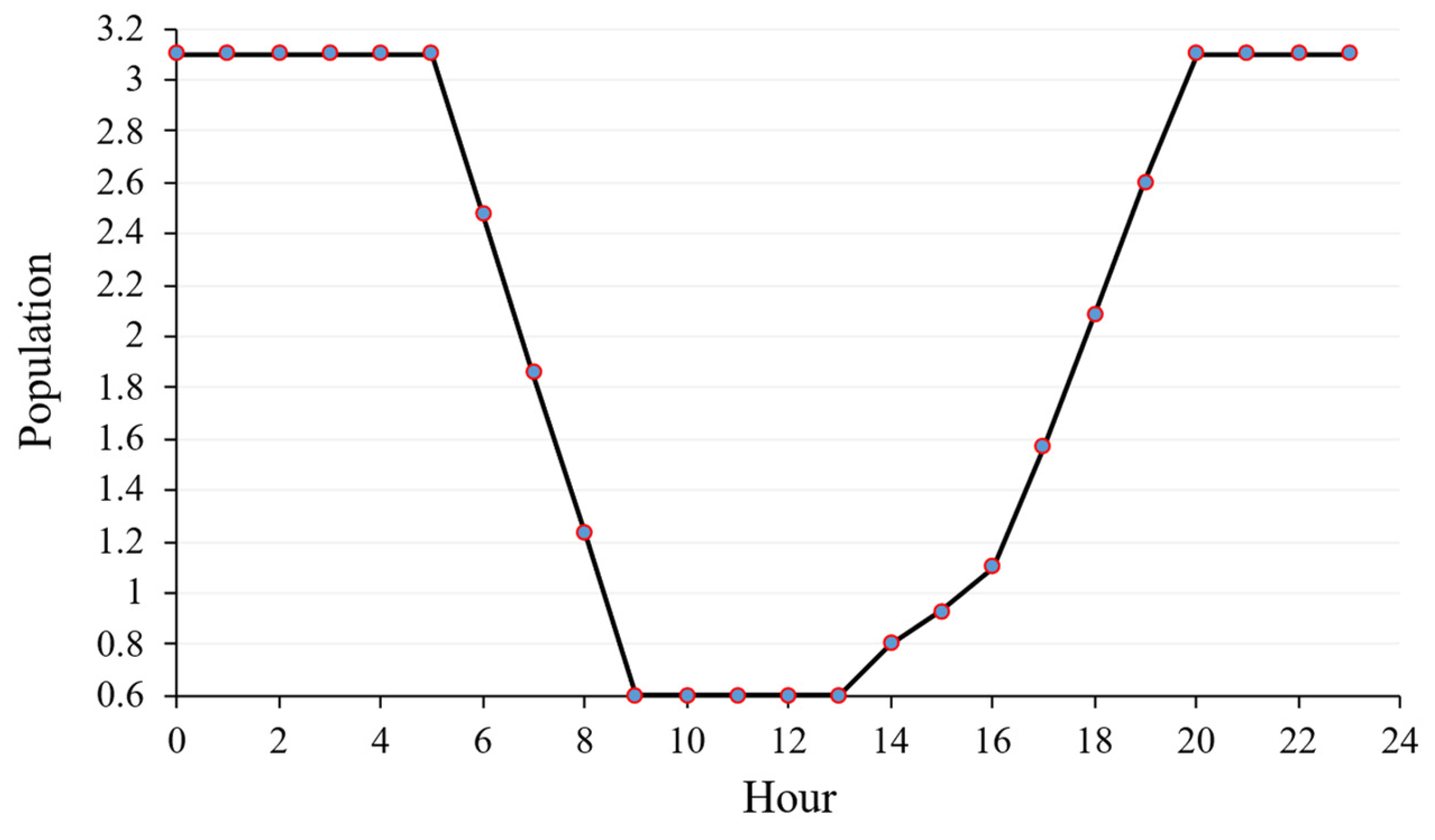
The building is classified as a multi-unit residential structure with an occupancy type corresponding to a peak of 3.1 occupants per 1000 square feet and a dispersion of 0.20. Figure 13 displays the weekday population distribution used in this analysis.
Following the population input, the next critical step involves detailing the structural and non-structural components of the building. This process is divided into two parts: (1) identification of the appropriate fragility groups for each storey, and (2) specification of the quantities of these components within designated functional groups. Fragility groups are present of components which have similar construction characteristics, including details of construction, details of manufacture, and installation techniques. PGs are a sub-categorisation of fragility groups and consist of components that experience the same type of demand (e.g., inter-storey drift or floor acceleration) and are characterised by a common fragility group identifier (ID). Fragility group IDs follow a structured classification. The first letter denotes the general category of components (e.g., B for structural elements), while subsequent digits specify the component type and configuration. For instance, “B10” refers to superstructure components, whereas “B20” designates exterior appendages. A full code such as “B1044” would refer to reinforced concrete shear walls, with decimal extensions used to denote variations in configuration, material properties, or installation conditions.
Table 3 lists all structural and non-structural components included in the analysis, along with their respective fragility IDs, demand types (EDPs), units, and quantities distributed across both floors and both structural directions (X and Y), as well as non-directional components (ND). Components sensitive to storey drift ratio (SDR) or peak floor acceleration (PFA) are included. Units are expressed in square feet (SF), linear feet (LF), or each (EA), depending on the nature of the component. Structural components (beams, columns, connections) were assigned fragility functions from the FEMA P-58 data library appropriate for ductile steel moment frames with RBS connections. Non-structural drift-sensitive components (e.g., drywall partitions, exterior curtain walls) were modelled with drift-based fragilities, while acceleration-sensitive components (e.g., suspended ceilings, mechanical/electrical equipment) used acceleration-based fragilities. For each hazard scenario, the MIDR and MFA obtained from the surrogate were input as demand parameters in PACT. Further details on how the component quantities in Table 3 were calculated and distributed across floors and directions are provided in the Supplementary Materials.
Employing Monte Carlo simulation (with 5000 realisations per scenario in this research), PACT produces probabilistic estimates for both repair costs and repair durations. In each realisation, the likelihood of each damage state for every component is sampled according to the fragility probability (based on the input EDP), and the corresponding consequences (repair costs and labour time) are extracted from established distributions. The result is a distribution of total repair costs and repair durations for the building. This study emphasises median (50th percentile) values as representative outcomes, which is a standard practice in performance evaluations.
In the scenario where only an earthquake is considered, the PACT analysis presumes the absence of flooding, thus the seismic demands are the sole contributors to damage. Conversely, in the scenario that combines earthquake and flooding, the demands encompass both the effects of the earthquake and those induced by flooding. The flood predominantly impacts the components on the first storey; for example, water pressures exert additional lateral forces and may lead to potential residual drift at this level, while inundation adversely affects the interior finishes and building systems located on the ground floor [23]. The repercussions of flooding were accounted for by evaluating the excessive demands it could impose on the drift values. For the sake of simplicity, the authors consider the flood damage to occur simultaneously with the aftermath of the earthquake, resulting in a singular damage assessment, as the flood event follows closely after. Any component that sustains damage from either hazard is deemed to require repair. In instances where a component’s fragility is not explicitly detailed in FEMA P-58, a rough estimation was employed. The structural repairs necessitated by the earthquake (such as the yielding of beams and minor yielding in certain connections) were further exacerbated by flood loading in the combined scenario, occasionally leading to more severe damage states or the collapse of non-structural infills. These influences were manifested in the surrogate-predicted increased drifts for the combined scenario, which subsequently resulted in elevated damage probabilities in the PACT analysis.

3.7. Delay Time Estimation via REDi Framework

PACT provides the direct repair time, i.e., the physical duration of repair assuming adequate workforce availability. However, it does not capture hindering factors that can significantly delay the start or progress of recovery. To account for these, this study adopts the REDi framework [12], which introduces standard durations for tasks such as:
  • Post-event inspections;
  • Engineering redesign and mobilisation;
  • Financing and insurance processing;
  • Contractor mobilisation;
  • Permitting and approvals.
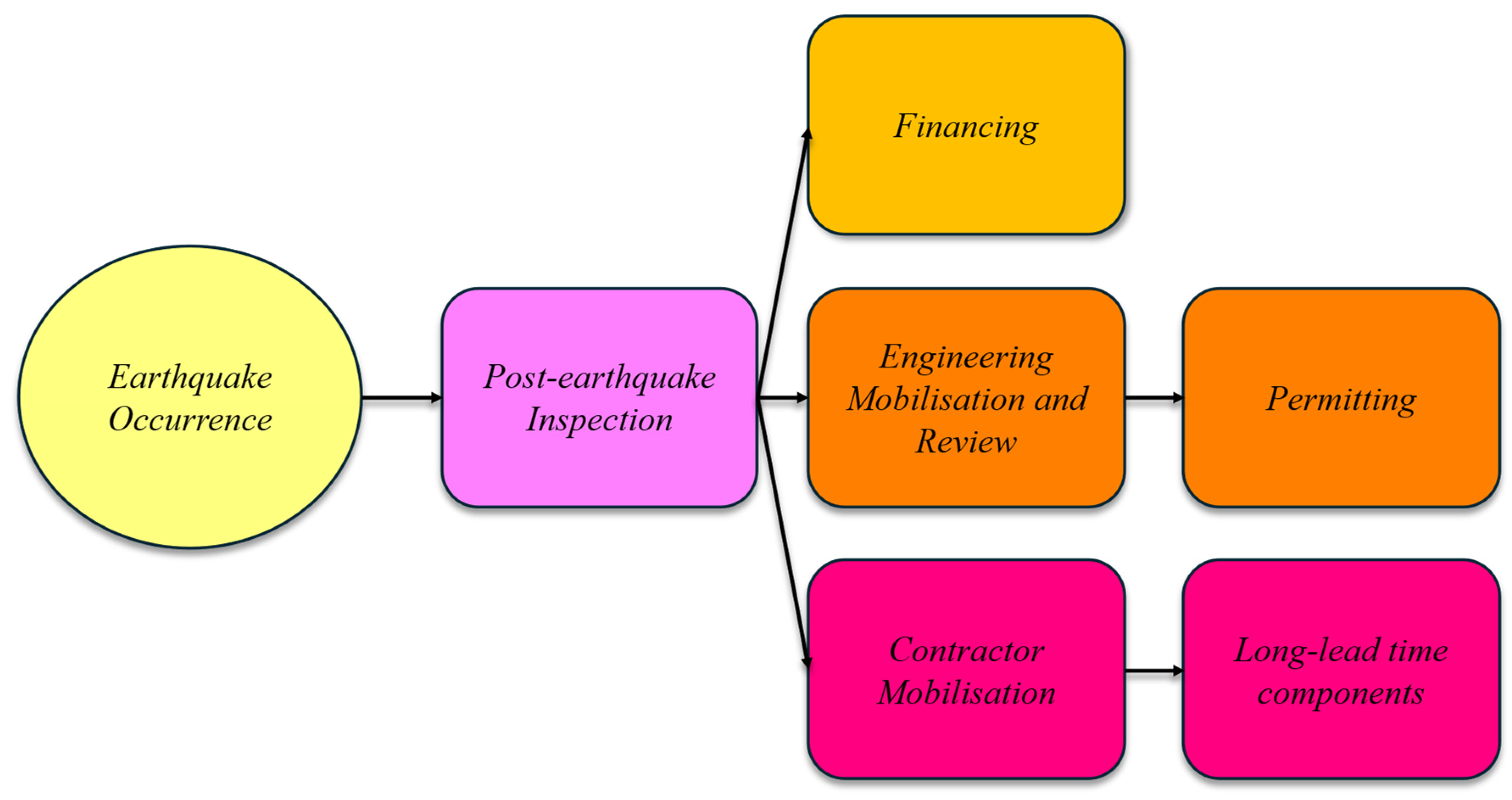
These factors are considered impediments because they postpone recovery. Delays are classified into categories depending on the type of damage (minor, non-structural, or major structural). REDi employs impeding delay curves for each task, and the total delay is determined by identifying the critical path (the longest sequence of dependent activities), rather than simply summing durations. Figure 14 depicts this logic, while Table 4 summarises the assumed impeding delays.
  • In the EQ-only scenario, the total delay prior to full restoration is several months. The most significant contributor is engineering and redesign, estimated at about 3 months.
  • In the EQ + FL = 4 m scenario, delays are considerably longer, particularly for engineering-related tasks, which increase to nearly 12 months due to the need for reassessment, redesign, and compliance with code upgrades following compounded damage.
  • Other factors such as financing, contractor mobilisation, permitting, and post-earthquake safety inspections (≈1 week) were assumed to be broadly similar across scenarios, since they are governed mainly by administrative processes. Although flood damage may complicate insurance claims, these were conservatively treated as equivalent in both cases.
It should be mentioned that the 350-day delay assumed for the EQ + Flood scenario was extracted directly from the REDi™ guideline, which provides impeding curves for engineering mobilisation and redesign following major seismic events. For buildings classified as extensive damage (Repair Class 3), the median delay is shown to reach 50 weeks (350 days). Given that sequential earthquake–flood events are expected to cause compounded structural impacts and necessitate substantial redesign and re-permitting, this value was adopted in the current study as the most representative estimate.
Based on the decision logic in Figure 14, three plausible sequences of delay events were analysed. The total delay was calculated as:
  • 166 days for the EQ-only scenario, and
  • 411 days for the EQ + FL = 4 m scenario.
These cumulative delays were then incorporated into the functionality curves, which provided the basis for estimating the Ri.

4. Results

4.1. Repair Cost

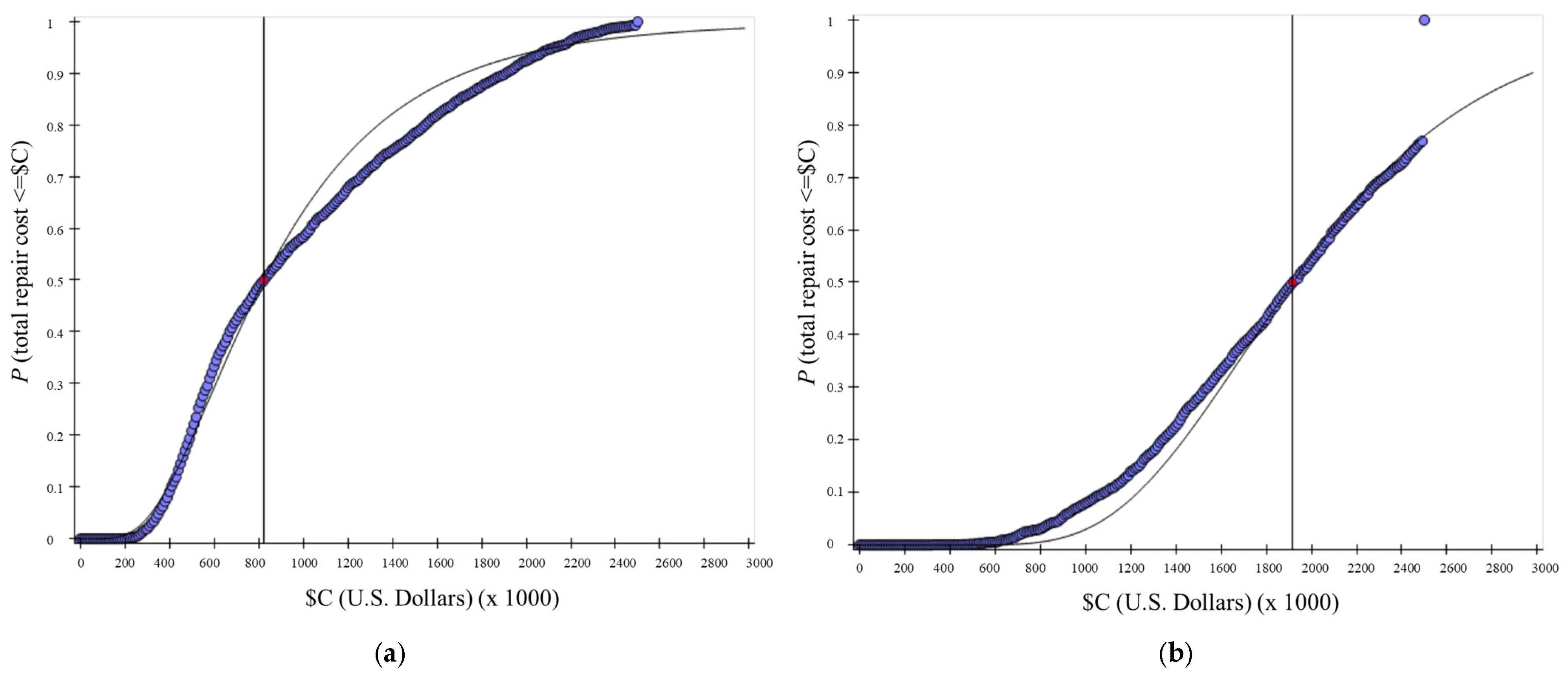
The discrepancies in damage are evident in the estimates for repair costs. In the case of the earthquake alone, the total estimated repair cost was approximately $0.82 million USD, representing about 33% of the building’s projected replacement value of $2.5 million. The primary factors contributing to this expense were non-structural elements: the replacement of cracked partition walls along with their finishes, repairs to exterior walls, curtain walls, and mechanical equipment, which collectively accounted for around 80% of the total cost. The remaining portion was attributed to structural repairs, predominantly concerning the RBS connection. Figure 15a depicts the cumulative distribution of repair costs for the earthquake-only scenario, revealing a 50% likelihood that repair expenses would not surpass nearly $0.82 million (the median), and a 90% probability that costs would remain below $1.8 million, with the variability in distribution stemming from uncertainties in damage outcomes. In stark contrast, the repair cost for the earthquake plus flood scenario escalates to approximately $1.92 million USD (median), which is about 77% of the overall replacement value. This represents a 133% increase in repair costs attributable to the flood’s effects. Essentially, in the combined scenario, the building is approaching a total loss, prompting many stakeholders to contemplate demolition and reconstruction, especially as repair costs near three-quarters of the replacement value [5]. Figure 15b illustrates the cost distribution for the combined scenario, which is biased towards higher losses; there exists a significant probability that the repair costs would meet or exceed the replacement costs, as certain simulations indicated that specific damage combinations rendered repairs economically unfeasible.
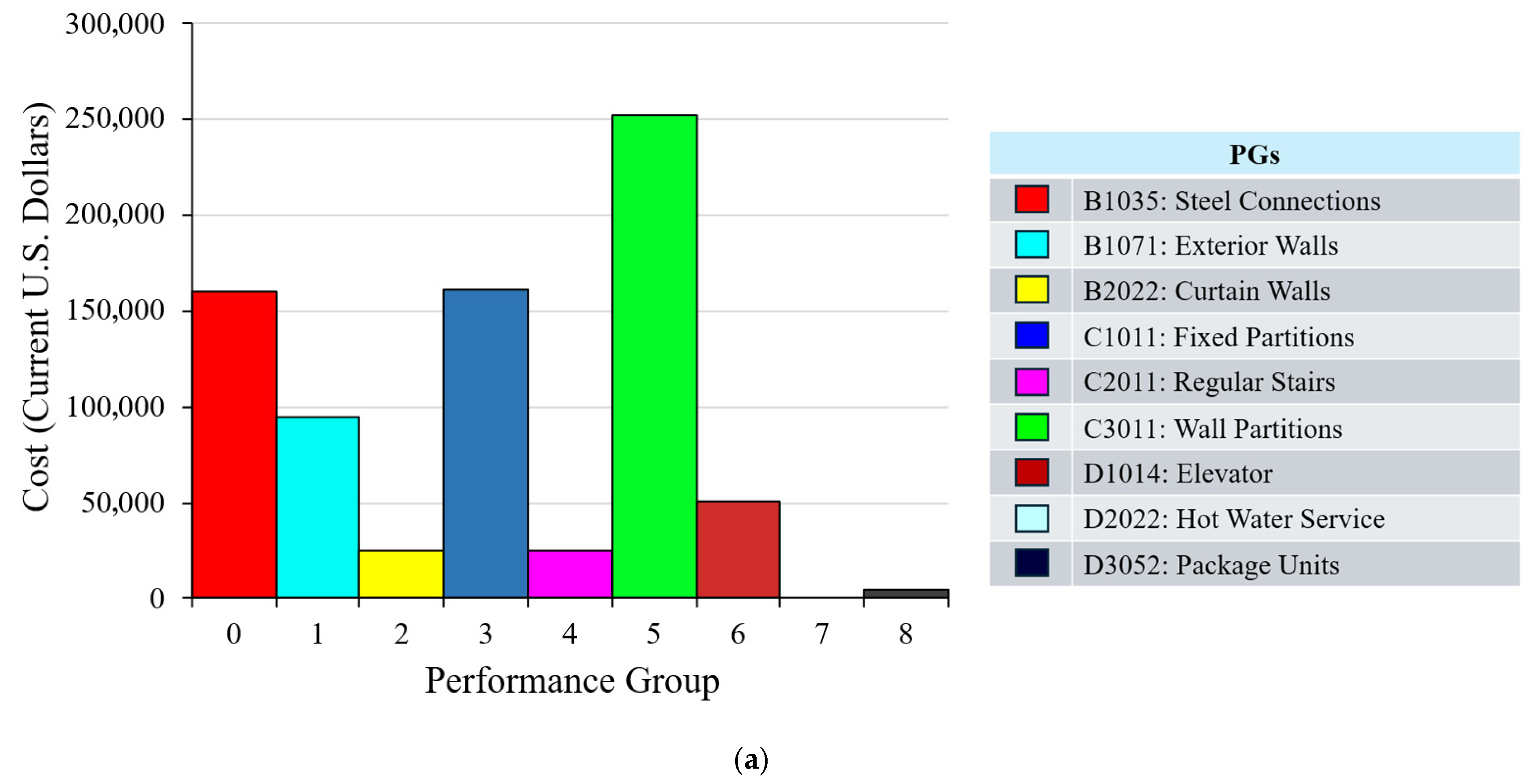
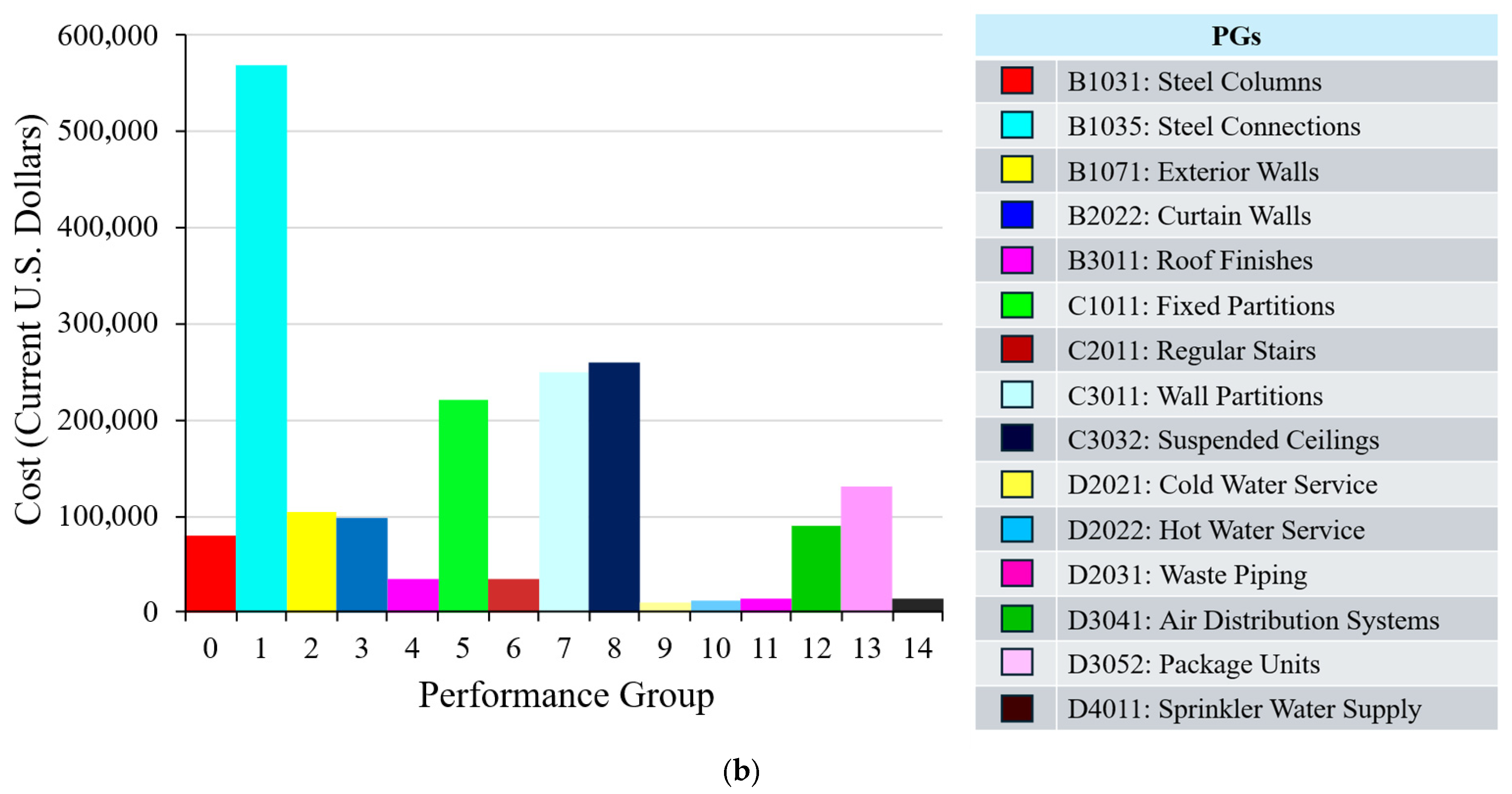
Analysing the costs by component category yields deeper understanding. Figure 16 presents a comparative analysis of repair cost breakdown by PG for the two scenarios. According to Figure 16a, in the earthquake-only scenario, the most significant single loss was attributed to partitions (both with and without finishes); for example, damage to interior partitions (fragility group C301) incurred costs of approximately $260k, while repairs for exterior walls (B107) amounted to about $93k. Damage to structural components (B103, which encompasses beam-to-column connections with RBS) was estimated at around $170k. In the combined EQ + FL scenario, every category experienced a substantial increase, as depicted in Figure 16b. Particularly, the repair costs for steel connections (B1035) surged to nearly $570k, which is almost 3.5 times higher than the costs observed in the earthquake-only scenario. This indicates that many connections that sustained damage during the earthquake ultimately became fractured or required replacement due to the additional loading from the flood. Likewise, while suspended ceilings exhibited minimal damage in the earthquake-only scenario, the flood caused extensive damage to all ground-floor ceilings; this, coupled with increased shaking on the upper floors, resulted in significant costs for the ceiling system in the combined scenario (ceiling damage escalated from nearly $0 to over $265k). Overall, structural repairs represented a larger proportion of the total costs in the EQ + FL scenario (approximately 33% of the total) compared to the EQ-only scenario (around 20%), with nearly every non-structural category experiencing cost increases of roughly two to three times. The necessity to replace mechanical and electrical systems due to flooding introduced a significant new expense in the EQ + FL scenario, contributing approximately $245k (whereas these costs were minimal in the EQ-only scenario). A comprehensive analysis of repair expenses categorised by PG for both hazard scenarios is presented in Table A2 and Table A3 in Appendix B, illustrating the cost contributions of structural and non-structural elements on each floor for the EQ only and EQ + FL = 4 m scenarios, respectively. These findings highlight how the flood intensified damage to both structural and non-structural components, significantly increasing repair requirements.

4.2. Repair Time and Downtime

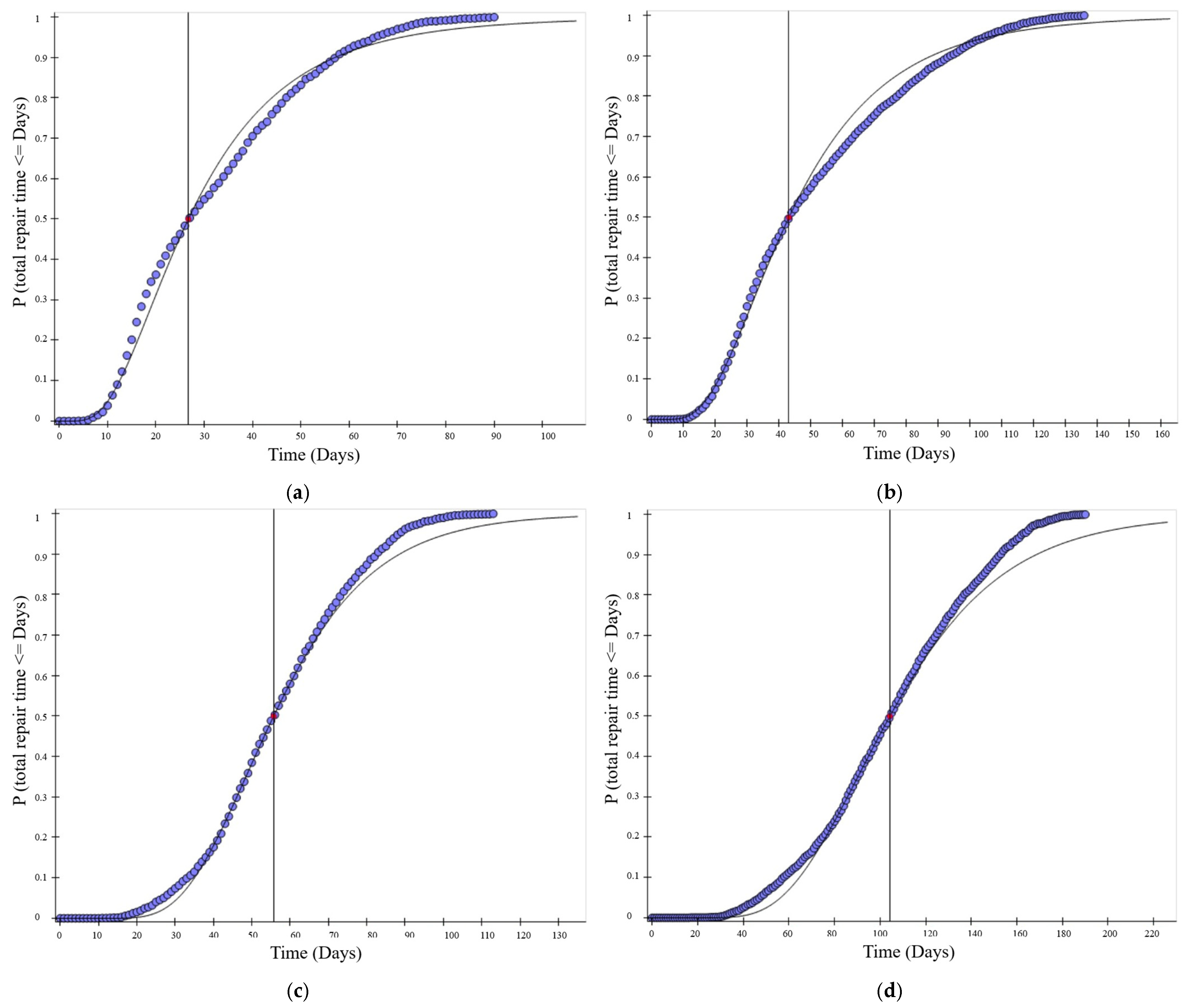
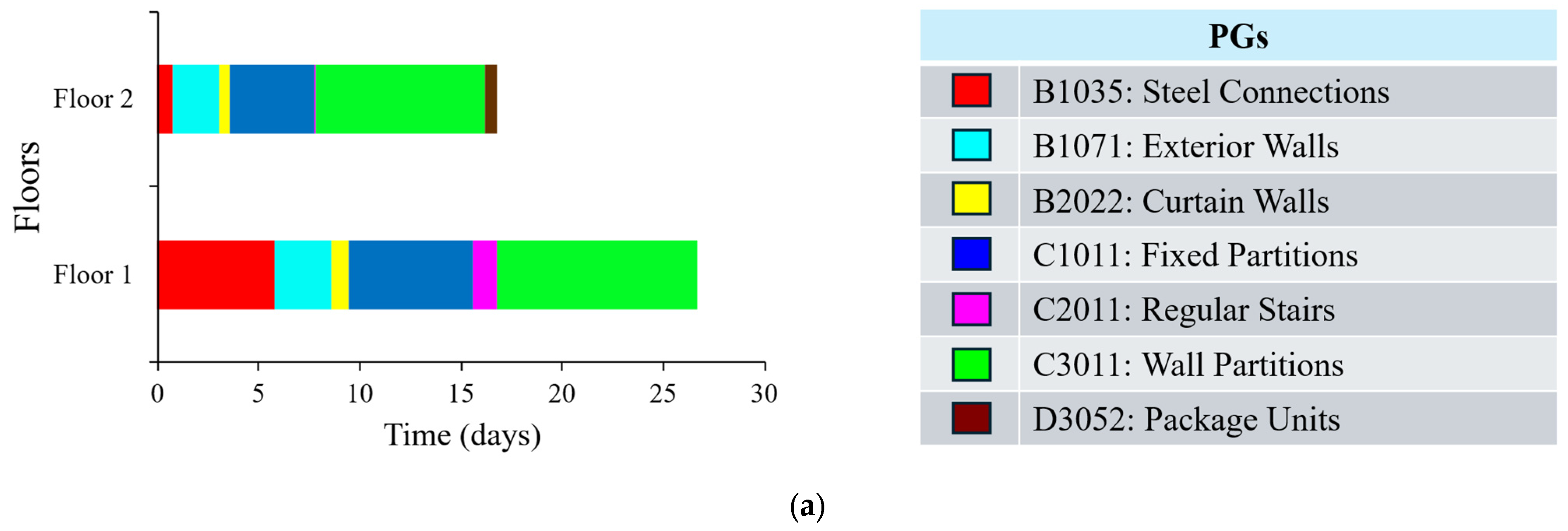
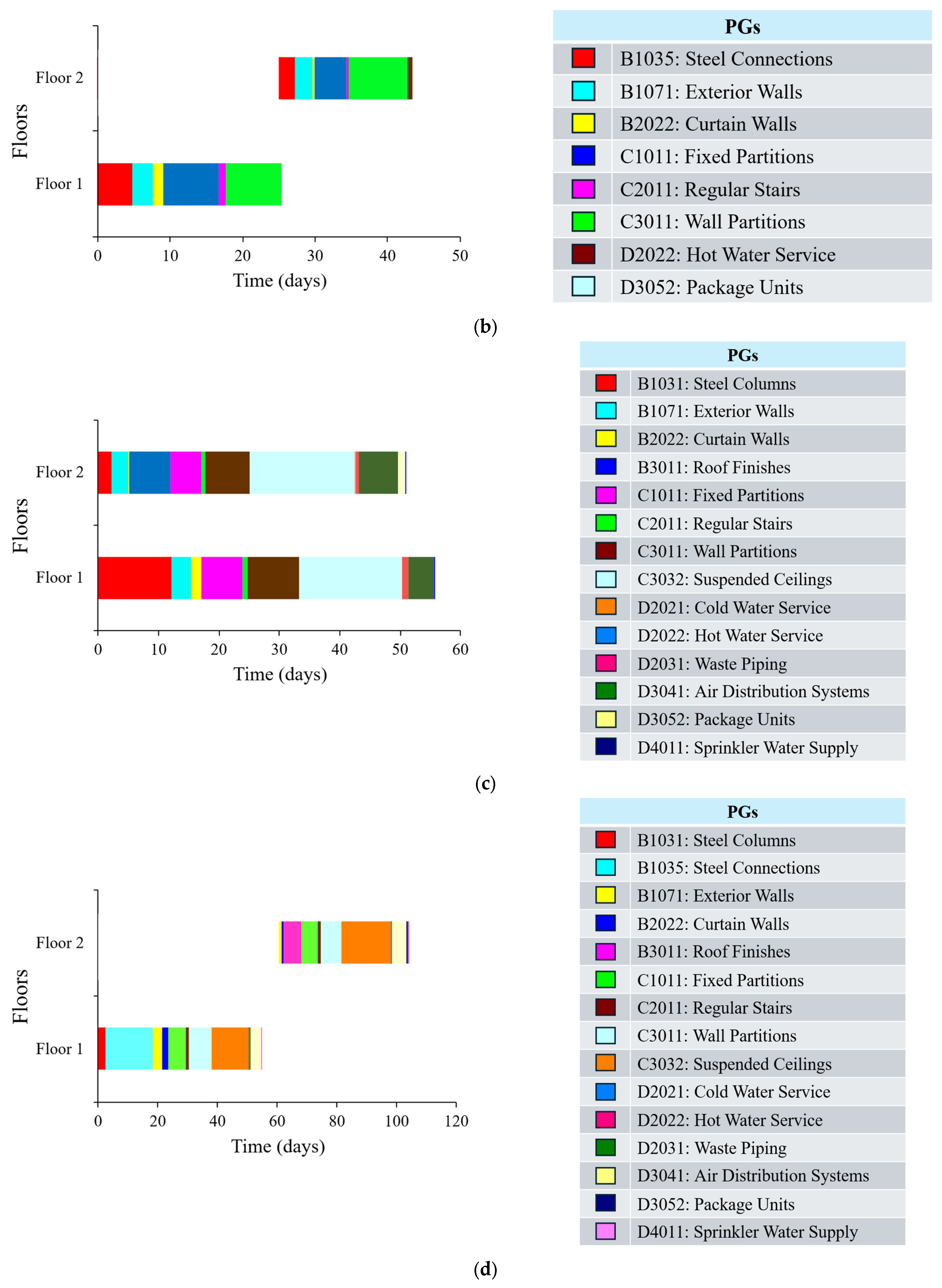
Repair time represents a vital metric in the assessment of resilience. PACT evaluates this in two distinct modes: (i) serial repair time, where repairs are conducted sequentially, floor by floor and (ii) parallel repair time, where repairs occur simultaneously across all floors. In the EQ-only scenario, illustrated in Figure 17a,b, the total repair duration is 26.72 days for the parallel approach and 43.35 days for the serial approach. In the combined EQ + FL = 4 m scenario, Figure 17c,d indicate that repair times escalate to 55.70 days and 104.24 days, respectively. This highlights a considerable delay attributed to flood-related damage, underscoring the necessity of multi-hazard evaluations in resilience planning. Component-level repair durations for both scenarios are detailed in Figure 18. According to Figure 18a,c, in the parallel repair scenario, the repair of wall partitions on the first storey took the longest, requiring 10 days in the EQ-only case, while in the EQ + FL = 4 m scenario, the most time-consuming task was the repair of the suspended ceiling on the second storey, which took nearly 18 days. The subsequent most time-intensive tasks included the repair of fixed partitions and steel connections on the first storey for the EQ-only scenario, and the repair of steel columns and wall partitions on the first storey for the EQ + FL = 4 m scenario. As shown in Figure 18b,d in the serial repair scenario, the longest tasks were the repair of wall partitions on the second storey (approximately 8 days) and the repair of the suspended ceiling on the second storey (approximately 17 days), which significantly influenced the overall repair timeline. Repair time estimates, divided by component and storey level, are listed for both serial and parallel repair scenarios in Table A4, Table A5, Table A6 and Table A7 in Appendix B. These tables present durations for each PGs, allowing for a detailed comparison between the EQ-only and EQ + FL = 4 m scenarios.
Together, these findings validate that flooding considerably intensifies both the magnitude and duration of damage in SMRF buildings subjected to seismic forces. As will be discussed in the subsequent sections, such effects also impact the Ri, which integrates both repair time and delay time to assess post-disaster recovery performance.
The detailed results presented in Appendix B Table A2, Table A3, Table A4, Table A5, Table A6 and Table A7 reinforce the main findings. For the EQ-only case (Table A2), the total repair cost was approximately USD 0.82M, with the largest contributions from steel connections, fixed partitions, and wall partitions. When a 4.0 m flood followed the earthquake (Table A3), costs nearly doubled to about USD 1.92M, reflecting additional damage to ground-floor systems such as suspended ceilings, piping, and sprinklers.
Repair durations show a comparable escalation. Under EQ-only conditions, expected recovery times were 26.71 days for parallel repairs (Table A5) and 43.35 days for series repairs (Table A4). With flood damage included, recovery time rose sharply to 55.70 days under parallel repairs (Table A7) and over 104.24 days under series repairs (Table A6). These results underline how cascading earthquake–flood hazards not only magnify repair costs but also extend recovery time by several months, primarily due to the compounded vulnerability of ground-floor structural and non-structural systems.
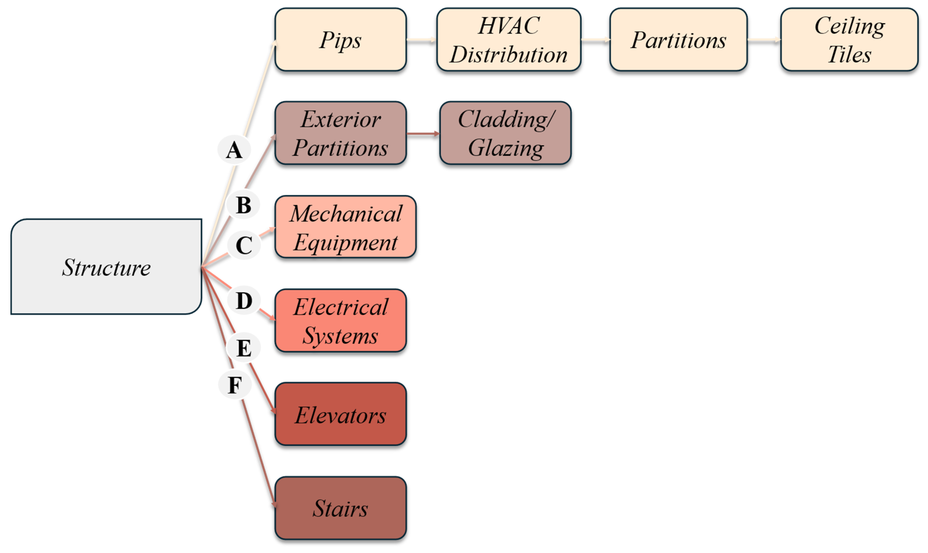
It is crucial to understand that PACT does not provide a specific or logical order for arranging component-level repair time bars in Figure 18. To address these inconsistencies and create a more realistic sequence of repair activities, this paper employs the REDi framework. The scheduling of repair work follows logical sequences based on the prioritisation recommended by REDi. Initially, all structural repairs are carried out to ensure safety for both occupancy and repair crews. Subsequently, non-structural repairs are conducted in parallel sequences: (A) interior partitions and piping, (B) exterior envelope, (C) mechanical systems, (D) electrical systems, (E) elevators, and (F) other life-safety systems, as illustrated in Figure 19. In an adequately resourced post-disaster reconstruction scenario, many of these tasks can be performed concurrently across different floors. The authors have assumed an optimistic scenario where multiple crews operate simultaneously on all floors for each sequence, meaning that the duration for each sequence is determined by the longest floor for that particular sequence. Consequently, the total repair time is the sum of the duration of structural repairs and the slowest non-structural sequence (given that sequences A–F are executed sequentially in a conservative scheduling approach, although some may overlap). Finally, the total downtime must be calculated by adding the delays identified in Table 4 to the direct repair time for each scenario.

4.3. Ri Comparison

Once all delays and repair durations have been established, the functionality recovery curve for the building can be derived. In both scenarios, the previously determined delay times (166 days for EQ-only and 411 days for EQ + FL = 4 m) are incorporated into the total repair time to ascertain the overall downtime. This downtime serves as the horizontal axis of the functionality curve. The vertical axis denotes functionality, commencing at 100% prior to the event, experiencing an immediate decline following the hazard event in relation to the repair cost as a fraction of the total replacement cost, and subsequently increasing linearly throughout the recovery phase until complete restoration is attained. Ri is calculated as the area beneath the functionality curve. Figure 20 depicts the functionality versus time curves for both scenarios. In the EQ-only scenario (Figure 20a), the repair cost constituted approximately 33% of the replacement cost, leading to the assumption that the building loses 33% of its functionality instantaneously after the earthquake. Consequently, the functionality curve drops immediately to 67% on Day 0 (the moment of the earthquake) and maintains that level during an initial delay of 166 days (impeding phase). Once repairs commence, functionality begins to improve as various systems are repaired. Initially, the repair of structural elements begins on the first floor and concludes on the second floor. Prior to this, no repairs are conducted on non-structural elements. Subsequently, non-structural repairs initiate simultaneously on both stories, commencing with sequence A and concluding with sequence F. By Day 194, all repairs are completed, and functionality is restored to 100%. The area beneath this curve is substantial, indicating that the building remained largely functional (albeit partially) for the majority of the duration.
In contrast, under the EQ + FL = 4 m scenario, the costs associated with repairs approach approximately 77% of the expenses for replacement, which effectively renders the building almost entirely non-functional (with an initial functionality loss of nearly 80%, indicating that only minimal operations can persist). Consequently, as illustrated in Figure 20b, the functionality curve for EQ + FL experiences a sharp decline to 20% performance on Day 0, coinciding with the occurrence of both the earthquake and flood. Following this event, the building remains in a state of reduced functionality throughout the subsequent delay phase of 411 days, as repairs have yet to commence. The structural repair process for storey 1 takes nearly 18 days, while storey 2 requires approximately 3 days to complete. Subsequently, the repair sequence A initiates concurrently at both stories, which takes about 40 days to finish. At this juncture, the damaged building is capable of restoring over 80% of its initial performance. It is only after approximately Day 480.25, when the major structural and system repairs are finalised, that functionality is restored to 100%.
The functionality curve, when plotted over time for each scenario, allows for the computation of Ri as the normalised area beneath the functionality–time curve up to a specified control time. In this context, the authors utilise the definition of Ri established by Cimellaro et al. [25], where TLC is defined as the maximum downtime of the two scenarios (in this instance, 480.25 days) to enable effective comparison. A hypothetical timeline of 480 days following the event is envisioned; ideally, a resilient building would recover swiftly and maintain full functionality for the majority of this duration, resulting in a high Ri value approaching 1. Conversely, a less resilient outcome would entail an extended period of functional loss, leading to a reduced area under the curve and consequently a lower Ri. The area beneath the recovery curve for each scenario is computed. The Ri for the earthquake-only scenario is determined to be 0.873 (87.3% resilience), signifying that, on average, the building retains 87% of its functionality over the 480-day reference period. Practically, this elevated Ri indicates a relatively resilient performance: despite sustaining damage, the building is expected to fully recover within approximately six months, and even during the repair phase, certain sections may remain operational. In contrast, for the EQ + FL scenario, the Ri is only 0.265, or about 26.5%. This suggests that, on average, during the 480 days following the event, the building operated at merely 27% of its pre-disaster capacity, effectively indicating that it was predominantly out of service for the duration of TLC.

5. Discussion

The above results highlight the profound effect that a cascading flood can have on the seismic resilience of a building. Several important observations and implications can be drawn:

5.1. Cascading Hazards Magnify Damage Nonlinearly

The damage resulting from the combination of an earthquake and flooding was not simply the aggregate of the effects of the two hazards; instead, it represented a compounding of their impacts. The earthquake rendered the structure significantly more susceptible to flood loads. For instance, the pre-existing plastic hinges in beams and connections had diminished stiffness and strength, leading to these components suffering considerably greater damage under flood pressures compared to an undamaged structure. The PACT results indicated that certain structural elements, such as RBS connections, experienced a loss that was 3 to 4 times greater in the combined scenario than in the case of the earthquake alone. This nonlinear amplification of damage aligns with intuitive understanding and highlights the risks associated with the assumption that separate designs for each hazard will guarantee safety when they occur together. Furthermore, it is consistent with findings from other multi-hazard research (for example, the impact of earthquakes following fires), where the damage from one hazard intensifies the effects of the subsequent hazard. For professionals in the field, this suggests that critical infrastructure located in multi-hazard areas should incorporate considerations of sequential loading in their design evaluations. Although current codes do not explicitly mandate this practice, resilience-based strategies should advocate for it.

5.2. Extended Downtime from Impeding Factors

A notable finding was the variation in delays encountered across different scenarios. In the combined scenario, the requirement for comprehensive engineering reassessment and redesign constituted the most significant delay (350 days, compared to 84 days for the EQ-only scenario). This underscores a somewhat overlooked aspect of resilience: in addition to physical repairs, the procedural and logistical hurdles following a major disaster can significantly extend recovery time. The application of the REDi framework facilitated the quantification of these elements. The results are consistent with those of Gallegos et al. [14] and others who stress that enhancements in design (to mitigate damage) must be paired with strategies for effective post-disaster decision-making to genuinely achieve expedited recovery. For instance, establishing pre-arranged contracts for emergency engineering services or contingency plans for permitting could significantly reduce that mobilisation delay. In our scenario, if the engineering/redesign delay could be reduced by half, the Ri would markedly improve. Consequently, resilience encompasses not only fortifying the structure but also optimising the post-event processes, a concept effectively encapsulated in REDi’s recommendations (e.g., pre-event mitigation strategies such as spare parts and emergency response plans).

5.3. Surrogate Modelling Efficacy

The surrogate models demonstrated their significant value in this research by facilitating a comprehensive analysis of loss and recovery in a complex multi-hazard context, all while avoiding excessive computational expenses. The Stack-AttenLSTM surrogate effectively forecasted the EDPs necessary for the FEMA P-58 loss assessments, eliminating the requirement for resource-intensive NLTHA through OpenSees simulation. This illustrates the practicality of employing sophisticated machine learning models in evaluations of multi-hazard resilience engineering. It adds to the burgeoning domain of artificial intelligence (AI)-enhanced structural engineering by broadening its application to sequential hazards, an area that has historically seen minimal investigation. The methodology can be adapted to various building types and combinations of hazards, such as integrating earthquakes with subsequent fires or aftershocks. One limitation is that surrogate models necessitate a substantial amount of training data that encompasses all pertinent physical phenomena; in this study, the generation of training data involved the integration of structural and fluid simulations, which is quite complex. Nevertheless, once the model is trained, it can swiftly assess numerous hazard intensities and scenarios. This capability could prove particularly advantageous for probabilistic risk assessments, which require thousands of hazard realisations.

5.4. Broader Impacts on Community Resilience

Although this analysis focuses on individual buildings, its implications reach into the realm of community resilience. When numerous structures within a city experience a sequential earthquake followed by a flood, the community’s recovery will be hindered by the slowest sector. The case study building required over a year to achieve full recovery in the context of a multi-hazard scenario. Should that building serve as a hospital or a power substation, the repercussions for the community would be significant. This emphasises the necessity of incorporating multi-hazard scenarios into resilience planning for essential infrastructure. As highlighted by Bonowitz [33], there have been suggestions to integrate resilience criteria into building evaluation standards. Our results strongly endorse such proposals: a building that meets “code-compliance” for life safety may still result in unacceptable downtime during a multi-hazard event, indicating the need for additional design objectives or retrofit triggers aimed at functional recovery, as also recommended in recent codes such as FEMA P-2090 [34].
In relation to existing design practice, current seismic codes such as ASCE 7 and AISC 341 provide detailed provisions for earthquake safety but do not explicitly address sequential hazards such as earthquake–flood events. Our findings demonstrate that meeting life-safety criteria alone does not guarantee acceptable functionality in compounded scenarios, reinforcing the argument for resilience-based objectives. The integration of FEMA P-58 and the REDi framework within our workflow illustrates how established performance-assessment tools can be adapted to multi-hazard contexts. Comparisons with alternative sequential hazard studies (e.g., earthquake–fire interactions) reveal consistent patterns of nonlinear amplification of damage, further supporting the need for multi-hazard provisions in practice. Looking forward, resilience strategies may include codifying flood-resistant detailing (e.g., water-resistant materials, sacrificial or replaceable structural fuses), embedding sequential hazard checks within FEMA P-58, or extending ASCE 7 objectives to explicitly address post-event functionality. Such measures would better align design standards with community resilience goals in regions exposed to cascading disasters.

5.5. Uncertainty Treatment

While this study applied Monte Carlo simulations to capture aleatory uncertainties in structural demand and loss estimation, epistemic sources of uncertainty also merit consideration. These include model-form assumptions, correlations between earthquake and flood hazards, and potential extrapolation limits of the surrogate models. To reduce extrapolation risks, surrogate training was restricted to ranges covered by validated FEMA P-695 databases [19], and predictions were cross-validated against unseen test sets. Nonetheless, future extensions could adopt Bayesian surrogate modelling to explicitly represent model-form uncertainty, copula-based methods to capture hazard correlations, and global sensitivity analyses to quantify uncertainty propagation across the framework. Incorporating such methods would further enhance confidence in multi-hazard resilience assessments.

5.6. Climate-Driven Cascading Hazards and Community-Scale Resilience

Recent studies on climate-driven multi-hazard risks highlight that structural resilience alone is insufficient without community-level adaptation and governance [35]. Evidence from flood-prone regions shows that weak infrastructure and limited institutional coordination can amplify cascading impacts [36]. Advances in artificial intelligence further demonstrate the potential for integrated early-warning systems that combine meteorological, geospatial, and socioeconomic data to anticipate complex climate risks. Survey results from U.S. municipalities also reveal that, despite progress in resilience and sustainability planning, explicit multi-hazard strategies remain underdeveloped [37]. These insights align with the findings of this study and suggest that building-level frameworks, such as the one proposed here, should ultimately be embedded within broader community-scale resilience planning and climate adaptation policies.
In conclusion, the discourse emphasises the importance of considering multi-hazard impacts in areas where such situations are likely to occur. The surrogate-based methodology illustrated in this context serves as an effective instrument for quantifying these impacts and can aid in performance-based engineering decisions that directly address resilience. By evaluating different design options through metrics like Ri, stakeholders are empowered to make well-informed decisions regarding investments in mitigation strategies (for instance, the installation of flood barriers or the incorporation of more durable structural features) based on their benefits in enhancing resilience.

6. Conclusions

This study extends our earlier surrogate modelling works [22,27] by moving beyond predictive accuracy and demonstrating their integration within a surrogate–PACT–REDi workflow for resilience assessment. The key contributions and findings are as follows:
  • Advanced data-driven surrogate models are effectively integrated with cutting-edge performance assessment (FEMA P-58) and recovery modelling (REDi) to assess not only the immediate damage caused by hazards but also the subsequent downtime and loss of functionality. This comprehensive approach facilitates the calculation of a quantitative Ri that reflects the cumulative impacts of multi-hazard events on building performance.
  • The resilience of the example SMRF building was markedly diminished by the occurrence of a flood following an earthquake. In numerical terms, the earthquake-only scenario yielded Ri = 0.87 (suggesting a relatively swift recovery, with full functionality restored in almost 6 months), while the sequential earthquake–flood scenario resulted in Ri = 0.27 (with full recovery taking nearly 16 months, during which the building was largely non-functional for the majority of that time). Repair expenses more than doubled, and downtime approximately doubled when the 4 m flood was added to the earthquake damage. These findings quantitatively validate the notion that cascading hazards can inflict significantly greater damage than isolated hazards, underscoring the necessity of designing and planning for such compound events.
  • The flood not only inflicted additional direct damage (especially to already compromised structural elements and unprotected non-structural systems) but also led to significant delays in recovery due to the necessity for redesign and coordination of repairs. Engineering re-evaluation emerged as a critical bottleneck in the combined scenario, indicating possible interventions (like pre-disaster planning, enhanced building inspection protocols, or modular design that accelerates post-flood repairs). The methodology identified the specific areas where time was lost (for instance, 350 days attributed to redesign delays), offering actionable insights for enhancing resilience, such as engaging in advance planning to manage post-disaster permitting and design modifications.
  • The significant disparity in results between the scenarios indicates that buildings designed according to current codes (which satisfy seismic life-safety standards) may exhibit inadequate performance during multi-hazard events, particularly regarding their functionality. There is a pressing necessity to integrate multi-hazard considerations into the design guidelines for essential structures. This integration could entail ensuring that both critical structural and non-structural elements are either robust or redundant in the face of compounded loading (for example, employing coatings or materials capable of withstanding inundation, or utilising structural fuses that can be readily replaced if they are overstressed by a subsequent hazard). The findings reinforce the advocacy for resilience-based design goals, which extend beyond mere life-safety to specifically aim for minimal downtime, particularly in areas prone to cascading disasters. Frameworks such as FEMA P-58 and REDi, when adapted to multi-hazard scenarios as demonstrated in this study, can provide a foundation for establishing such objectives.
  • Beyond the specific case studied, the framework provides a generalisable methodology for resilience assessment. It can be extended to reinforced concrete (RC) structures, tall buildings, and critical facilities by training surrogate models tailored to their configurations. Furthermore, the approach is adaptable to other sequential or compound hazards, such as earthquake–hurricane or earthquake–fire scenarios, where cascading effects are expected to amplify damage and recovery demands. Exploring these extensions will help advance resilience-based design and inform future updates to performance-based codes and standards.
  • As one of the limitations, it can be mentioned that in the current framework, flood duration and rise time were not explicitly considered, which represents a limitation for scenarios involving long-lasting or slowly rising inundation. Also, future work could extend the framework by incorporating time-dependent hydrographs into the CFD analyses, allowing the surrogate models to capture effects of sustained flooding, gradual rise, or receding waters. Another limitation of the present framework is that flood-specific non-structural damage mechanisms (e.g., equipment corrosion, soaked finishes, or long-term material degradation due to water exposure) were not explicitly modelled. Following the assumptions of prior multi-hazard studies [23,27], non-structural elements such as infill walls were considered to fail during the seismic phase, leaving the residual flood capacity governed primarily by beams, columns, and connections. Accordingly, the surrogate models focused on MIDR and MFA, which are the EDPs most relevant to FEMA P-58 fragility definitions. While this approach adequately captures the instantaneous effects of sequential earthquake–flood loading, it does not represent long-duration flooding. Future extensions could integrate additional fragilities or explicitly model non-structural deterioration under sustained inundation to improve the realism and comprehensiveness of resilience assessments. Finally, future extensions of this work could explore the use of advanced, structure-specific and multi-modal intensity measures, such as modal-weighted Sa, Saavg over period bands, and spectral shape parameters (e.g., ε at T1) [38,39,40], to further enhance surrogate prediction efficiency, robustness, and sufficiency.
In summary, the assessment of resilience based on surrogates provides a robust mechanism for engineers and researchers to analyse and enhance building performance in the context of intricate hazard scenarios. The case study highlights the essential requirement to design not only for singular hazards but also for their interactions, in order to prevent significant losses in functionality. By proactively tackling multi-hazard risks and emphasising swift recovery, it is possible to progress towards genuinely resilient buildings and communities. It is advisable that forthcoming building regulations and retrofit recommendations integrate multi-hazard resilience standards, and that additional research be undertaken on a broader spectrum of structures to develop a thorough understanding of multi-hazard effects. The methodologies outlined in this study can support such research by allowing for detailed yet efficient simulations of hypothetical scenarios. Ultimately, investing in designs that are resilient to multiple hazards is expected to yield benefits in terms of diminished economic losses and enhanced safety amidst increasingly complex natural hazard threats.

Supplementary Materials

The supporting information describing the process used to extract the values reported in Table 3 from FEMA P-58 Volumes 1 and 2 can be downloaded at: https://www.mdpi.com/article/10.3390/buildings16010048/s1.

Author Contributions

Conceptualization, D.S. and I.B.M.; Methodology, D.S. and I.B.M.; Software, D.S.; Validation, D.S. and I.B.M.; Formal Analysis, D.S.; Investigation, D.S.; Resources, D.S. and I.B.M.; Data Curation, D.S. and I.B.M.; Writing—Original Draft Preparation, D.S.; Writing—Review & Editing, D.S. and I.B.M.; Visualization, D.S. and I.B.M.; Supervision, I.B.M.; Project Administration, I.B.M. All authors have read and agreed to the published version of the manuscript.

Funding

This research received no external funding.

Institutional Review Board Statement

Not applicable.

Informed Consent Statement

Not applicable.

Data Availability Statement

The data presented in this study are available on request from the corresponding author. In addition, the PACT input files for both the EQ-only and EQ + FL scenarios have been provided as Supplementary Materials. These files include all model parameters, fragility components, ground motion records, EDP values, hazard curves, repair costs, and repair times, enabling independent verification and reproducibility of the results. In addition, the surrogate models developed for the EQ-only scenario and the EQ + FL scenario have been made publicly available at https://github.com/DelbazSamadian/Surrogate-Model-for-SMRF (accessed on 13 July 2025). and https://stack-atten-lstm-sm.streamlit.app/ (accessed on 13 July 2025).

Conflicts of Interest

The authors declare no conflicts of interest.

Appendix A. CFD Analysis in OpenFOAM

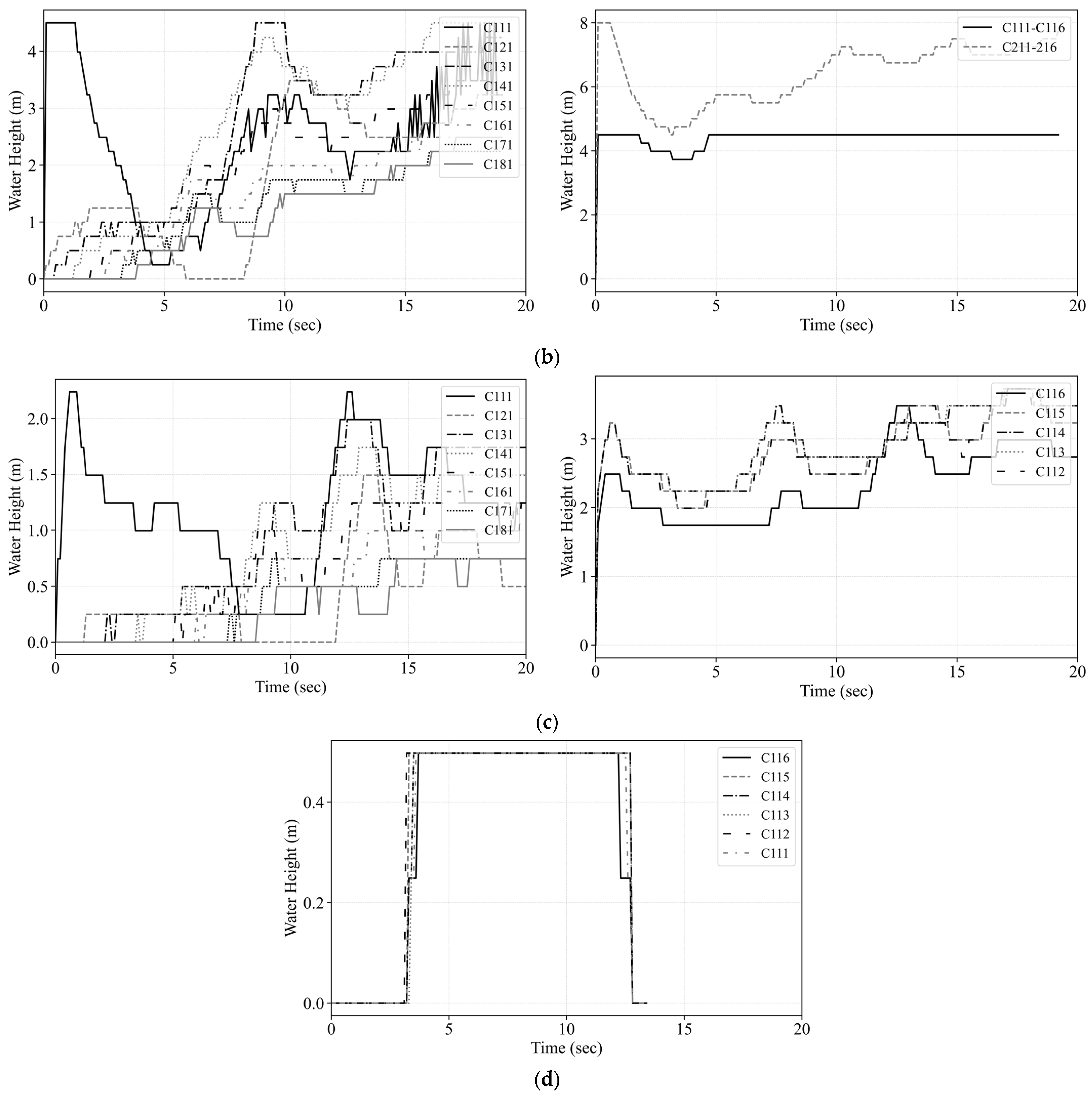
Flood-induced structural demands are frequently assessed using simplified approaches such as the Equivalent Lateral Load (ELL) and Variable Depth Pushover (VDPO) methods [41,42,43,44,45]. These rely on static pressure distributions derived from assumed inundation depths and are useful for preliminary assessments. However, they fail to represent the transient and nonlinear nature of flood actions, which involve turbulence, wave impact, and complex fluid–structure interactions [23]. Important dynamic effects, including turbulence, flow separation, eddy formation, and fluctuating pressures, are neglected, often resulting in under- or overestimation of structural response. To overcome these limitations, high-fidelity computational fluid dynamics (CFD) analyses are required to capture the complete flood–structure interaction process [46].
In this study, three-dimensional CFD modelling is performed in OpenFOAM, which can handle free-surface, multiphase flows and complex geometries. Simulations are carried out for 2-, 8-, and 20-storey SMRF buildings, with representative geometries derived from group averages. The models are first generated and meshed in ANSYS 2024R2 [47] and subsequently exported to OpenFOAM for flow simulation (setup illustrated in Figure A1a). The computational domain reproduces a dam-break flood event [23], representing the sudden release of water toward the building. Four inlet-to-structure distances are investigated (2, 5, 10, and 20 m), with results showing that 5–10 m provides consistent hydrodynamic behaviour. A distance of 5 m is selected as the default case, balancing numerical convergence and physical realism (Figure A1a). For broader modelling considerations, particularly earthquake–flood–structure interaction frameworks, readers are referred to Reference [23].
Figure A1. Set up for the flood water impacting the 2-storey SMRF building: (a) set up of the reservoir in OpenFOAM; (b) computational mesh [23].
Buildings 16 00048 g0a1
For the 2-storey configuration, the simulation domain extends 52.70 m × 40.60 m × 8.40 m, incorporating a 5 m clearance buffer around the structure and a 1 m-wide upstream water column to ensure sufficient initial fluid volume (Figure A1a). Flood turbulence is modelled using the Reynolds-Averaged Navier–Stokes (RANS) framework with the standard k–ε turbulence model, which solves transport equations for turbulent kinetic energy and dissipation rate. This model offers a practical compromise between numerical stability and the ability to capture dominant flow features in large-scale, multiphase simulations.
The interFoam solver is employed to resolve air–water interactions through the Volume of Fluid (VoF) method. In this formulation, each computational cell is assigned a phase fraction (α1) indicating water, air, or a mixed state. The solver explicitly incorporates surface tension, buoyancy, and gravitational forces, making it particularly suited for simulating free-surface phenomena such as wave breaking, splashing, and interface deformation.
  • Boundary Conditions, Meshing, and Solver Settings
Boundary conditions and initial states are defined to replicate realistic fluid behaviour. Solid surfaces are treated with no-slip conditions, while the outlet and top boundaries represent atmospheric exposure and open water flow, respectively. Near-wall turbulence effects are captured using standard wall functions.
Mesh generation is performed in ANSYS 2024R2 using a hybrid strategy: structured hexahedral elements are applied where feasible to enhance spatial accuracy, with local refinement concentrated near the building façade and the air–water interface. A base cell size of 0.25 m is adopted, providing sufficient resolution of pressure gradients without incurring prohibitive computational cost (Figure A1b).
Time advancement follows the Courant–Friedrichs–Lewy (CFL) stability condition, with adaptive time stepping used to maintain a maximum Courant number of 0.5. Pressure–velocity coupling is handled by the PIMPLE algorithm, which combines features of the PISO and SIMPLE schemes to improve robustness for unsteady multiphase flows. For selected simulations, the k–ω SST turbulence model is applied to enhance resolution of shear layers and transitional flow regions near surfaces.
  • Inlet Conditions and Output for Structural Modelling
Flood forcing is introduced through depth-dependent inlet velocity profiles, representing realistic variations in wave height and flow intensity. The simulations track the temporal evolution of pressures and velocities at critical structural interfaces, yielding high-resolution data for force extraction. Outputs include spatially and temporally distributed hydrodynamic quantities, specifically: (i) total pressure forces along the X, Y, and Z directions, and (ii) rotational moments about all three axes. These results are post-processed into force profiles that provide input features for surrogate model training.
A comprehensive summary of CFD setup parameters, including turbulence models, boundary conditions, and numerical schemes, is presented in Table A1. This high-fidelity CFD workflow enables the generation of realistic flood loading scenarios, thereby supporting accurate and generalisable predictions of structural performance under sequential earthquake–flood hazards.
  • Hydrodynamic Load Extraction and Structural Interaction Effects
To illustrate flood-induced structural behaviour, this Section examines the two-storey SMRF as a representative case. This choice balances detail with brevity; broader comparisons across multiple building heights are available in [23], which show consistent response trends primarily governed by building height. Hydrodynamic analysis is limited to members in direct contact with the fluid domain, with flood loads assigned only to beams and columns that are partially or fully submerged based on the evolving water surface profile.
A systematic notation is adopted for structural components to facilitate analysis. Columns are denoted by “C” and beams by “B,” followed by three digits indicating the storey level (j), horizontal index (i), and depthwise position (k). For example, C213 refers to a column on the second storey (j = 2), at grid location i = 1, k = 3. Floodwater interaction patterns and inundation progressions across different flood heights (FH) are visualised in Figure A2 using OpenFOAM results.
Time-series analyses are conducted to track force evolution under varying flood heights. Figure A3 presents the flood height histories acting on 2-storey building columns at different intensity levels. Hydrodynamic forces extracted from OpenFOAM include: (i) drag forces (Fx), acting parallel to the flood flow; (ii) lift forces (Fy, Fz), acting vertically and laterally; and (iii) moments (My), arising from asymmetric pressure distributions along member height. According to the CFD results, columns directly facing the incoming flood, particularly ground-level members, experience the largest demands. At a peak flood depth of 4 m, drag forces on front-facing ground columns reach nearly 900,000 N, before tapering to ~250,000 N as velocities decrease. Lift forces, generally 750–2000 N, display similar temporal decay but contribute substantially to overturning, especially under asymmetric flow. Associated bending moments about the vertical axis can exceed 8,000,000 Nm, indicating strong torsional stresses.
Flow visualisation also reveals vortex shedding effects, notably behind the first column row. For instance, C111, the leading column, experiences lower peak loads than downstream columns such as C121 or C131 due to wake formation and localised low-pressure regions. These effects amplify secondary loads on trailing members, a phenomenon often neglected in static flood force methods. Comparable behaviour is observed in beams. First-storey beams exposed to the flood front initially sustain drag forces approaching 750,000 N, with impacts diminishing as water advances downstream. Lift forces of 2000–3000 N, combined with asymmetric fluid momentum transfer, generate significant bending and torsional demands.
Results consistently show that increasing inundation depth intensifies both the magnitude and spatial distribution of hydrodynamic actions across the frame. These findings highlight the necessity of capturing time-varying, multi-directional, and rotational flood loads, particularly for lower storeys and directly impacted members.
Figure A2. OpenFOAM simulation for the 2-storey SMRF with FH = 4 m at: (a) 1 sec; (b) 5 sec; (c) 10 sec; (d) 20 sec [23].
Buildings 16 00048 g0a2
Figure A3. Time history of flood flow on columns for the 2-storey SMRF buildings at different flood levels: (a) FH = 4 m; (b) FH= 2 m; (c) FH = 1 m; (d) FH = 0.30 m [23].
Buildings 16 00048 g0a3aBuildings 16 00048 g0a3b
Table A1. Boundary conditions defined in OpenFOAM [23].
Boundary α ϵ k n u t n u T i l d a p _ r g h U
InletvariableHeightFlowRatefixedValuefixedValuecalculatedzeroGradientzeroGradientvariableHeightFlowRateInletVelocity
OutletzeroGradientinletOutletinletOutletcalculatedzeroGradientzeroGradientzeroGradient
RightzeroGradientepsilonWallFunctionkqRWallFunctionnutkWallFunctionzeroGradientfixedFluxPressurenoSlip
LeftzeroGradientepsilonWallFunctionkqRWallFunctionnutkWallFunctionzeroGradientfixedFluxPressurenoSlip
BottomzeroGradientepsilonWallFunctionkqRWallFunctionnutkWallFunctionzeroGradientfixedFluxPressurenoSlip
AtmosphereinletOutletinletOutletinletOutletcalculatedzeroGradienttotalPressurepressureInletOutletVelocity
BuildingzeroGradientepsilonWallFunctionkqRWallFunctionnutkWallFunctionzeroGradientfixedFluxPressurenoSlip

Appendix B

Table A2. Repair costs (in U.S. dollars) by PG for the EQ-only scenario.
StoreyB1035: Steel ConnectionB1071: Exterior WallsB2022: Curtain WallsC1011: Fixed PartitionsC2011: Regular StairsC3011: Wall PartitionsD1014: ElevatorD2022: Hot WaterD3052: Package UnitsTotal Repair Cost
1125,953.780849,240.734727,641.4221109,637.951523,435.47192127,142.927156,00000822,624.965
246,983.2133643,196.55955196.8120763,299.431698502.988245133,793.67201002500
Sum of PG172,936.99492,437.29432,838.234172,937.38331,938.460260,936.59956,0001002500
Table A3. Repair costs (in U.S. dollars) by PG for the EQ + FL = 4 m.
StoreyB1031: Steel ColumnB1035: Steel ConnectionB1071: Exterior WallsB2022: Curtain WallsB3011: Wall PartitionsC1011: Fixed PartitionsC2011: Regular StairsC3011: Wall PartitionsC3032: Suspended CeilingD2021: Cold WaterD2022: Hot WaterD2031: Waste PipingD3041: Air Distribution SystemD3052: Package UnitsD4011: Sprinkler Water SupplyTotal Repair Cost
168,000.00455,540.6157,827.7067,153.390.00112,924.0125,417.66130,982.16113,578.66527.993658.035425.5934,134.0202956.8821,917,607.702
20.00110,459.6549,772.4232,846.3242,000.21106,075.6524,582.65118,017.65154,421.47472.0184341.363574.6547,865.36141,000.364051.232
Sum of PG68,000.00566,000.26107,600.1299,999.7142,000.21218,999.6650,000.31248,999.81268,000.131000.0087999.399000.2481,999.38141,000.367000
Table A4. Recovery time (days) for series repair of the 2-storey SMRF building under the EQ-only scenario.
StoreyB1035: Steel ConnectionB1071: Exterior WallsB2022: Curtain WallsC1011: Fixed PartitionsC2011: Regular StairsC3011: Wall PartitionsD2022: Hot WaterD3052: Package UnitsSum of StoreyTotal Repair Time
14.8382.8041.4387.6391.0287.5970025.344
21.8052.4600.2724.4110.3747.9950.2010.48918.00743.351
Sum of PG6.6435.2641.71012.0501.40215.5920.2010.489
Table A5. Recovery time (days) for parallel repair of the 2-storey SMRF building under the EQ-only scenario.
StoreyB1035: Steel ConnectionB1071: Exterior WallsB2022: Curtain WallsC1011: Fixed PartitionsC2011: Regular StairsC3011: Wall PartitionsD3052: Package UnitsSum of StoreyTotal Repair Time
15.790112.839760.828006.177911.19049.89152026.717726.7177
20.788212.304460.467284.16980.128478.291060.6651816.8145
Max of PG5.790112.839760.828006.177911.19049.891520.66518
Table A6. Recovery time (days) for series repair of the 2-storey SMRF building under the EQ + FL = 4 m scenario.
StoreyB1031: Steel ColumnB1035: Steel ConnectionB1071: Exterior WallsB2022: Curtain WallsB3011: Roof FinishesC1011: Fixed PartitionsC2011: Regular StairsC3011: Wall PartitionsC3032: Suspended CeilingD2021: Cold WaterD2022: Hot WaterD2031: Waste PipingD3041: Air Distribution SystemD3052: Package UnitsD4011: Sprinkler Water SupplySum of StoreyTotal Repair Time
12.44115.7813.3981.77206.0230.9637.80312.1230.0220.0190.6533.46300.16254.622
203.8272.9250.8675.6545.6580.9317.03116.4820.0190.0220.4304.8560.6940.22349.619104.241
Sum of PG2.44119.6076.3232.6395.65411.6811.89414.83428.6040.0410.0411.0838.3190.6940.385
Table A7. Recovery time (days) for parallel repair of the 2-storey SMRF building under the EQ + FL = 4 m. scenario.
StoreyB1035: Steel ConnectionB1071: Exterior WallsB2022: Curtain WallsB3011: Roof FinishesC1011: Fixed PartitionsC2011: Regular StairsC3011: Wall PartitionsC3032: Suspended CeilingD2021: Cold WaterD2022: Hot WaterD2031: Waste PipingD3041: Air Distribution SystemD3052: Package UnitsD4011: Sprinkler Water SupplySum of StoreyTotal Repair Time
112.1443.2641.60506.8360.9028.60416.9240.0150.0191.0104.24600.13155.700
22.3062.6110.3116.6755.1250.7247.27617.5080.0500.0250.6326.4621.1100.16150.97655.70
Max of PG12.1443.2641.6056.6756.8368.6048.60417.5080.0500.0251.0106.4621.1100.161

References

  1. Jonkman, S.N.; Vrijling, J.K. Loss of Life due to Floods. J. Flood Risk Manag. 2008, 1, 43–56. [Google Scholar] [CrossRef] [Scilit]
  2. Vanneste, K.; Camelbeeck, T.; Verbeeck, K.; Demoulin, A. Morphotectonics and Past Large Earthquakes in Eastern Belgium. In Landscapes and Landforms of Belgium and Luxembourg; World Geomorphological Landscapes; Demoulin, A., Ed.; Springer: Cham, Switzerland, 2018; pp. 215–236. [Google Scholar] [CrossRef] [Scilit]
  3. Puthanpurayil, A.M.; Jury, R.; D Hooper, J.; Carr, A. Code Based Design vs. Performance Based Design. In Proceedings of the 2024 New Zealand Society for Earthquake Engineering Annual Technical Conference, Wellington, New Zealand, 9–11 April 2024. [Google Scholar]
  4. Abate, M.; Evangelista, A.C.J.; Tam, V.W. Advanced Seismic Analysis of a 44-Story Reinforced Concrete Building: A Comparison of Code-Based and Performance Based Design Approaches. Infrastructures 2025, 10, 93. [Google Scholar] [CrossRef] [Scilit]
  5. Applied Technology Council, and National Earthquake Hazards Reduction Program (US). Seismic Performance Assessment of Buildings; Federal Emergency Management Agency: Washington, DC, USA, 2012.
  6. Jarrett, J.A.; Judd, J.P.; Charney, F.A. Comparative evaluation of innovative and traditional seismic-resisting systems using the FEMA P-58 procedure. J. Constr. Steel Res. 2015, 105, 107–118. [Google Scholar] [CrossRef] [Scilit]
  7. Guerrero, H.; Terán-Gilmore, A.; Ji, T.; Escobar, J.A. Evaluation of the economic benefits of using buckling-restrained braces in hospital structures located in very soft soils. Eng. Struct. 2017, 136, 406–419. [Google Scholar] [CrossRef] [Scilit]
  8. Liu, B.; Lu, Y.; Li, W.; Li, J.; Zhao, J.; Wang, S.; Ni, G.; Meng, Q. Study on seismic behavior of different forms of eccentrically braced steel frames. Buildings 2024, 14, 2064. [Google Scholar] [CrossRef] [Scilit]
  9. Ghods, B.; Rofooei, F.R. Seismic design of buildings in the context of regions: A case study of a site in Semnan city, Iran. Soil Dyn. Earthq. Eng. 2024, 186, 108891. [Google Scholar] [CrossRef] [Scilit]
  10. Safiey, A.; Majdalaweyh, S.; Pang, W. Assessing the impact of ground motion duration on losses in typical modern steel moment frames. Buildings 2024, 14, 1373. [Google Scholar] [CrossRef] [Scilit]
  11. Ramírez, W.; Mayacela, M.; Contreras, L.; Iza, N.; Quishpe, E.; Rentería, L. Economic seismic performance of buildings with PEER methodology and FEMA P-58. Buildings 2023, 13, 2259. [Google Scholar] [CrossRef] [Scilit]
  12. Almufti, I.; Willford, M. Resilience-Based Earthquake Design Initiative (REDi™) for the Next Generation of Buildings; ARUP: San Francisco, CA, USA, 2013; pp. 1–133. [Google Scholar]
  13. Terzic, V.; Villanueva, P.K.; Saldana, D.; Yoo, D.Y. Framework for modelling post-earthquake functional recovery of buildings. Eng. Struct. 2021, 246, 113074. [Google Scholar] [CrossRef] [Scilit]
  14. Gallegos, M.F.; Araya-Letelier, G.; Lopez-Garcia, D.; Molina Hutt, C. Loss and downtime assessment of RC dual wall–frame office buildings toward resilient seismic performance. Sustainability 2025, 17, 1200. [Google Scholar] [CrossRef] [Scilit]
  15. Takaya, K.; Jin, J.; Nagae, T. Practical repair cost assessment of steel office buildings with diverse beam-to-column connection types in Japan. Buildings 2024, 14, 3913. [Google Scholar] [CrossRef] [Scilit]
  16. Samadian, D.; Muhit, I.B.; Dawood, N. Application of Data-Driven Surrogate Models in Structural Engineering: A Literature Review. Arch. Comput. Methods Eng. 2024, 32, 735–784. [Google Scholar] [CrossRef] [Scilit]
  17. FEMA. Seismic Performance Assessment of Buildings—Implementation Guide; FEMA P-58-2; Federal Emergency Management Agency: Washington, DC, USA, 2012.
  18. Guan, X. Performance-Based Analytics-Driven Seismic Design of Steel Moment Frame Buildings. Doctoral Dissertation, University of California, Los Angeles, CA, USA, 2021. University of California Los Angeles Theses and Dissertations Archive. Available online: https://escholarship.org/uc/item/5bd6r600 (accessed on 25 July 2023).
  19. Applied Technology Council. Quantification of Building Seismic Performance Factors; US Department of Homeland Security, FEMA: Washington, DC, USA, 2009.
  20. American Institute of Steel Construction. Seismic Provisions for Structural Steel Buildings; American Institute of Steel Construction (AISC): Chicago, IL, USA, 2005; ANSI/AISC; AISC 341-05; Available online: https://www.aisc.org/Seismic-Provisions-for-Structural-Steel-Buildings-ANSIAISC-341-05-and-ANSIAISC-341s1-05-2005 (accessed on 14 December 2025).
  21. American Society of Civil Engineers. Minimum Design Loads and Associated Criteria for Buildings and Other Structures; ASCE 7-05; ASCE: Reston, VA, USA, 2006. [Google Scholar] [CrossRef] [Scilit]
  22. Samadian, D.; Muhit, I.B.; Occhipinti, A.; Dawood, N. Surrogate models for seismic and pushover response prediction of steel special moment resisting frames. Eng. Struct. 2025, 314, 118307. [Google Scholar] [CrossRef] [Scilit]
  23. Samadian, D.; Eslamnia, H.; Muhit, I.B.; Pregnolato, M.; Dawood, N. An Integrated Framework for 3D Time History Analysis of Steel Special Moment-Resisting Frame Buildings under Sequential Flood and Earthquake Hazards. Struct. Infrastruct. Eng. 2025, 1–24. [Google Scholar] [CrossRef] [Scilit]
  24. Bruneau, M.; Chang, S.E.; Eguchi, R.T.; Lee, G.C.; O’Rourke, T.D.; Reinhorn, A.M.; Shinozuka, M.; Tierney, K.; Wallace, W.A.; Von Winterfeldt, D. A framework to quantitatively assess and enhance the seismic resilience of communities. Earthq. Spectra 2003, 19, 733–752. [Google Scholar] [CrossRef] [Scilit]
  25. Cimellaro, G.P.; Reinhorn, A.M.; Bruneau, M. Framework for analytical quantification of disaster resilience. Eng. Struct. 2010, 32, 3639–3649. [Google Scholar] [CrossRef] [Scilit]
  26. Samadian, D.; Occhipinti, A.; Muhit, I.B.; Dawood, N. Stack-AttenLSTM: A Surrogate Deep Learning Model for Sequential Earthquake-Flood Vulnerability Assessment of Steel Buildings. Eng. Struct. 2025. under review. [Google Scholar]
  27. Ancheta, T.D.; Darragh, R.B.; Stewart, J.P.; Seyhan, E.; Silva, W.J.; Chiou, B.S.J.; Wooddell, K.E.; Graves, R.W.; Kottke, A.R.; Boore, D.M.; et al. NGA-West2 Database. Earthq. Spectra 2014, 30, 989–1005. [Google Scholar] [CrossRef] [Scilit]
  28. Samadian, D.; Fayaz, J.; Muhit, I.B.; Dawood, N. Structural Failure Analysis with CMS-Based Ground Motion Selection Using Innovative Cost Function and Weight Factors. Earthq. Eng. Eng. Vib. 2025. ahead of print. [Google Scholar] [CrossRef] [Scilit]
  29. Su, R.K.L.; Lee, C.L. Development of seismic fragility curves for low-rise masonry infilled reinforced concrete buildings by a coefficient-based method. Earthq. Eng. Eng. Vib. 2013, 12, 319–332. [Google Scholar] [CrossRef] [Scilit]
  30. FEMA; NIBS. HAZUS Earthquake Model Technical Manual (Version 6.1); National Institute of Building Sciences: Washington, DC, USA; Federal Emergency Management Agency: Washington, DC, USA, 2024.
  31. Güner, T.; Topkaya, C. Performance comparison of BRBFs designed using different response modification factors. Eng. Struct. 2020, 225, 111281. [Google Scholar] [CrossRef] [Scilit]
  32. R.S. Means Company. Building Construction Costs with RSMeans Data (Annual ed.); Gordian RSMeans Data: Greenville, SC, USA, 2016. [Google Scholar]
  33. Bonowitz, D. Resilience criteria for seismic evaluation of existing buildings: A proposal to supplement ASCE 31 for intermediate performance objectives. In Proceedings of the ATC & SEI 2009 Conference on Improving the Seismic Performance of Existing Buildings and Other Structures, San Francisco, CA, USA, 9–11 December 2009; pp. 477–488. [Google Scholar]
  34. NIST; FEMA. Recommended Options for Improving the Built Environment for Post-Earthquake Reoccupancy and Functional Recovery Time; FEMA P-2090/NIST SP-1254; National Institute of Building Sciences: Washington, DC, USA; Federal Emergency Management Agency: Washington, DC, USA, 2020.
  35. Malecha, M.; Calvin, C.; Walpole, E. How well are US communities planning for resilience, climate adaptation, and sustainability—And what’s missing? Results of a national survey of local staff and officials. J. Environ. Plan. Manag. 2025, 68, 2438–2456. [Google Scholar] [CrossRef] [Scilit]
  36. Reichstein, M.; Benson, V.; Blunk, J.; Camps-Valls, G.; Creutzig, F.; Fearnley, C.J.; Han, B.; Kornhuber, K.; Rahaman, N.; Schölkopf, B.; et al. Early warning of complex climate risk with integrated artificial intelligence. Nat. Commun. 2025, 16, 2564. [Google Scholar] [CrossRef] [Scilit] [PubMed]
  37. Niraula, M.P.; Pandey, D.C.L.; Pariyar, R.K. Community Resilience to Multi-Hazard Risks: Insights from the Narayani Basin, Nepal. arXiv 2025. [Google Scholar] [CrossRef] [Scilit]
  38. Kalapodis, N.A.; Muho, E.V.; Beskos, D.E. Structure-specific, multi-modal and multi-level scalar intensity measures for steel plane frames. Soil Dyn. Earthq. Eng. 2025, 190, 109185. [Google Scholar] [CrossRef] [Scilit]
  39. Tothong, P.; Luco, N. Probabilistic seismic demand analysis using advanced ground motion intensity measures. Earthq. Eng. Struct. Dyn. 2007, 36, 1837–1860. [Google Scholar] [CrossRef] [Scilit]
  40. Luco, N.; Cornell, C.A. Structure-specific scalar intensity measures for near-source and ordinary earthquake ground motions. Earthq. Spectra 2007, 23, 357–392. [Google Scholar] [CrossRef] [Scilit]
  41. Kelman, I. Physical Flood Vulnerability of Residential Properties in Coastal, Eastern England. Doctoral Dissertation, University of Cambridge, Cambridge, UK, 2022. Available online: https://ilankelman.org/phd/IlanKelmanPhDDissertation.pdf (accessed on 10 January 2024).
  42. Federal Emergency Management Agency. Engineering Principles and Practices for Retrofitting Flood-Prone Residential Structures; Federal Emergency Management Agency (FEMA): Washington, DC, USA, 2012; FEMA P-259.
  43. Tagle, S.J.; Jünemann, R.; Vásquez, J.; de la Llera, J.C.; Baiguera, M. Performance of a Reinforced Concrete Wall Building Subjected to Sequential Earthquake and Tsunami Loading. Eng. Struct. 2021, 238, 111995. [Google Scholar] [CrossRef] [Scilit]
  44. Petrone, C.; Rossetto, T.; Baiguera, M.; De la Barra Bustamante, C.; Ioannou, I. Fragility Functions for a Reinforced Concrete Structure Subjected to Earthquake and Tsunami in Sequence. Eng. Struct. 2020, 205, 110120. [Google Scholar] [CrossRef] [Scilit]
  45. Attary, N.; Van De Lindt, J.W.; Barbosa, A.R.; Cox, D.T.; Unnikrishnan, V.U. Performance-Based Tsunami Engineering for Risk Assessment of Structures Subjected to Multi-Hazards: Tsunami Following Earthquake. J. Earthq. Eng. 2021, 25, 2065–2084. [Google Scholar] [CrossRef] [Scilit]
  46. Le, T.T.H.; Nguyen, V.C.; Nguyen, D.T.; Tran, D.T. Coupling CFD Model and FEM Model to Investigate the Impact of Debris Flows on a Low-Rise Building. Results Eng. 2024, 24, 103063. [Google Scholar] [CrossRef] [Scilit]
  47. ANSYS 2024R2. Available online: https://www.ansys.com/en-gb (accessed on 10 April 2024).
Figure 1. (a) Workflow for extracting resilience index (Ri) for single- and multi-hazard scenarios using the FEMA P-58 methodology; (b) Streamlined workflow for resilience assessment of SMRF buildings under sequential earthquake–flood hazards.
Buildings 16 00048 g001aBuildings 16 00048 g001b
Figure 2. Reference buildings of 2-storey building. (Left): Illustration depicting a plan view of SMRFs, including tributary seismic mass, gravity load, and leaning columns. (Right): Elevation view of the SMRF showcasing bay length and story height.
Buildings 16 00048 g002
Figure 3. FEMA P-58 damage assessment process used in this study.
Buildings 16 00048 g003
Figure 4. Framework for extracting Ri. TOE: time of event occurrence (e.g., earthquake or earthquake + flood), TRE: recovery time required to restore functionality, and TLC: control time used for calculating Ri. The shaded area under the curve corresponds to Ri.
Buildings 16 00048 g004
Figure 5. Prediction results using 13 ML methods on 2-storey meta database for (a) MIDR; (b) MFA [22].
Buildings 16 00048 g005
Figure 6. Scatter graph for the prediction results of MIDR using CatBoost for 2-storey SMRF building [22].
Buildings 16 00048 g006
Figure 7. Graphical User Interface (GUI) for MIDR estimation for NLTHA predictions for the 2-storey SMRF building [22].
Buildings 16 00048 g007
Figure 8. Evaluation of prediction performance for MIDR. (a) Comparison of average prediction accuracy across three different random seeds (45, 50, 60) shows that the ground truth model (Stack-AttenLSTM) outperforms both alternative models, achieving the highest R2 value (0.879) with lower MAE and RMSE. (b) The scatter plot illustrates a strong alignment between predicted and actual MIDR values for the ground truth model, with points closely scattered around the ideal prediction line, confirming its superior generalisation and accuracy.
Buildings 16 00048 g008
Figure 9. Workflow of the surrogate model for estimating MIDR in the 2-storey SMRF building subjected to sequential flood–earthquake hazards: (a) Application overview and usage instructions; (b) Importing the ground motion record in the horizontal X direction; (c) Importing the ground motion record in the horizontal Y direction; (d) Entering the 10 most influential input features; (e) Estimating MIDR using the developed Stack-AttenLSTM model.
Buildings 16 00048 g009aBuildings 16 00048 g009b
Figure 10. Ground motion selection using modified- CMS for the 2-storey SMRF building.
Buildings 16 00048 g010
Figure 11. Linear regression of MIDR values obtained from surrogate models for: (a) EQ only; (b) EQ + FL = 4 m.
Buildings 16 00048 g011
Figure 12. Fragility curves for the 2-storey SMRF for damage states of slight, moderate, and extensive under: (a) EQ only; (b) EQ + FL = 4 m.
Buildings 16 00048 g012
Figure 13. Population distribution for a multi-unit residential building in PACT.
Buildings 16 00048 g013
Figure 14. Sequence of delay due to impeding factors.
Buildings 16 00048 g014
Figure 15. Cumulative distribution of total repair costs for the 2-storey SMRF building at the DBE hazard level: (a) EQ-only scenario; (b) EQ + FL = 4 m scenario. Flooding nearly doubles the median repair cost (from ~33% to ~77% of replacement value), pushing the building close to total economic loss.
Buildings 16 00048 g015
Figure 16. Repair costs by PG for the 2-storey SMRF building: (a) EQ-only scenario; (b) EQ + FL = 4 m scenario. Flooding amplifies costs across nearly all categories, with steel connections and ground-floor systems showing the sharpest increases.
Buildings 16 00048 g016aBuildings 16 00048 g016b
Figure 17. Cumulative distribution of total repair time for the 2-storey SMRF building: (a) parallel repair, EQ-only scenario; (b) series repair, EQ-only scenario; (c) parallel repair, EQ + FL = 4 m; (d) series repair, EQ + FL = 4 m. Flooding approximately doubles expected repair durations, highlighting delays in restoring functionality.
Buildings 16 00048 g017
Figure 18. Repair time by PG for the 2-storey SMRF building: (a) parallel repair, EQ-only scenario; (b) series repair, EQ-only scenario; (c) parallel repair, EQ + FL = 4 m scenario; (d) series repair, EQ + FL = 4 m scenario. Flooding shifts the critical repair path from wall partitions to ground-floor structural and ceiling systems, prolonging overall downtime.
Buildings 16 00048 g018aBuildings 16 00048 g018b
Figure 19. Typical repair sequences at each floor level. Structural repairs must be completed before non-structural systems, underscoring how compounded flood damage delays later recovery phases.
Buildings 16 00048 g019
Figure 20. Functionality curve and Ri for the 2-storey SMRF building: (a) EQ-only scenario; (b) EQ + FL = 4 m scenario. Flooding reduces initial functionality by nearly 80% and extends downtime from 194 to over 411 days, cutting the Ri by two-thirds.
Buildings 16 00048 g020
Table 1. Member sizes for beams and columns for the 2-storey SMRF building.
StoreyBeam SizeExterior Column SizeInterior Column Size
1W30X132W24X131W24X162
2W16X31W24X131W24X162
Table 2. Information for the 2-storey SMRF building as defined in PACT.
Building InformationValueReference
Total replacement cost$2,500,000[30]
Core and shell replacement cost$500,000[7,31]
Replacement time357 days[6]
Total loss threshold1[30]
Maximum workers/per square foot0.001[9]
Floor area14,066 sq. ft[32]
Storey height (Floor 1)14.76 ft[32]
Storey height (Floor 2)12.80 ft[32]
Table 3. Structural and non-structural components and their quantities in PACT for the 2-storey SMRF building.
No.Fragility IDComponentEDPUnitX-1X-2Y-1Y-2ND-1ND-2
1B2022.001Curtain wallsSDR30 SF40.9640.9629.3629.3600
2B3011.011Concrete tile roofSDR100 SF0000045
3C1011.001aGypsum wall partitionSDR100 LF9.839.837.057.0500
4C3011.001aGypsum wall partition + WallpaperSDR100 LF3.113.112.232.2300
5C3032.001aSuspended ceiling, SDC A, B, CPFA250 SF000056.2656.26
6D2021.012aCold or hot potable, SDC CPFA1000 LF00001.551.55
7D3041.011bHVAC ducting—less than 6 sq. ft section area, SDC CPFA1000 LF00000.7030.703
8D3041.031aHVAC Drops/Diffusers, SDC A, BPFA10 EA000011.2511.25
9D3041.041aVariable air volume SDC, A, BPFA10 EA00002.82.8
10D4011.022aFire-sprinkler water piping, SDC CPFA1000 LF00003.093.09
11D4011.032aFire-sprinkler drop, SDC CPFA100 EA00001.691.69
12B1035.001Post-Northridge RBS connection beam depth < W27—one sideSDREA444400
13B1035.011Post-Northridge RBS connection beam depth < W27—both sidesSDREA444400
14B1035.002Post-Northridge RBS connection beam depth >= W30—one sideSDREA444400
15B1035.012Post-Northridge RBS connection beam depth >= W30—both sidesSDREA444400
16C2011.001bPrefabricated steel stairs—no seismic jointSDREA110000
17D1014.011Traction elevator-1976 or laterPFAEA000010
18D3052.011aAir handling unit—Capacity: <5000 CFM—Unanchored equipmentPFA4000 CFM0000010
19D5012.021aLow voltage switchgear—Capacity: 100 to <350 Amp—Unanchored equipmentPFAEA00002.100
20C3011.002aWall partition, Type: Gypsum + Ceramic TileSDR100 LF3.113.112.232.2300
21D2022.12aHeating hot water piping—Small diameter, SDC CPFA1000 LF00001.551.55
22D2031.012bSanitary waste piping, SDC CPFA1000 LF00001.691.69
23B1071.041Exterior wallSDR100 SF2.802.802.012.0100
24B1031.011aSteel column base plates, Column W < 150 plfSDREA808000
Table 4. Impeding factors estimated based on the REDi framework for the 2-storey SMRF building (days).
ScenarioPost-Earthquake InspectionsEngineering Mobilisation and Review/Re-DesignFinancingContractor Mobilisation and Bid ProcessPermitting
EQ only584716156
EQ + FL = 4 m5350716156
Disclaimer/Publisher’s Note: The statements, opinions and data contained in all publications are solely those of the individual author(s) and contributor(s) and not of MDPI and/or the editor(s). MDPI and/or the editor(s) disclaim responsibility for any injury to people or property resulting from any ideas, methods, instructions or products referred to in the content.