Proxy-Calibration Approach for Transient Simulation of Variable Refrigerant Flow Systems in Energy Performance Assessment of an Existing Building

Abstract
1. Introduction
2. Target Building Description
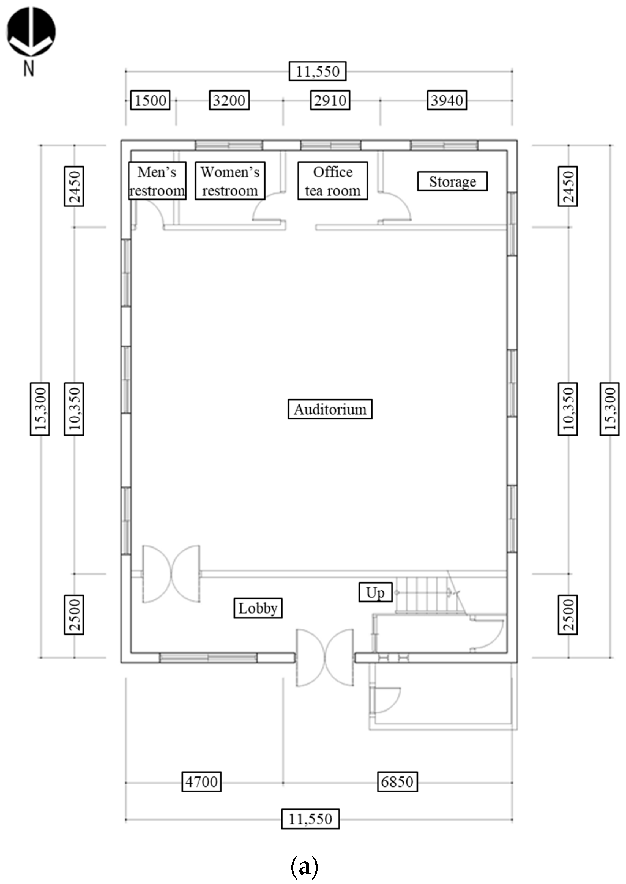
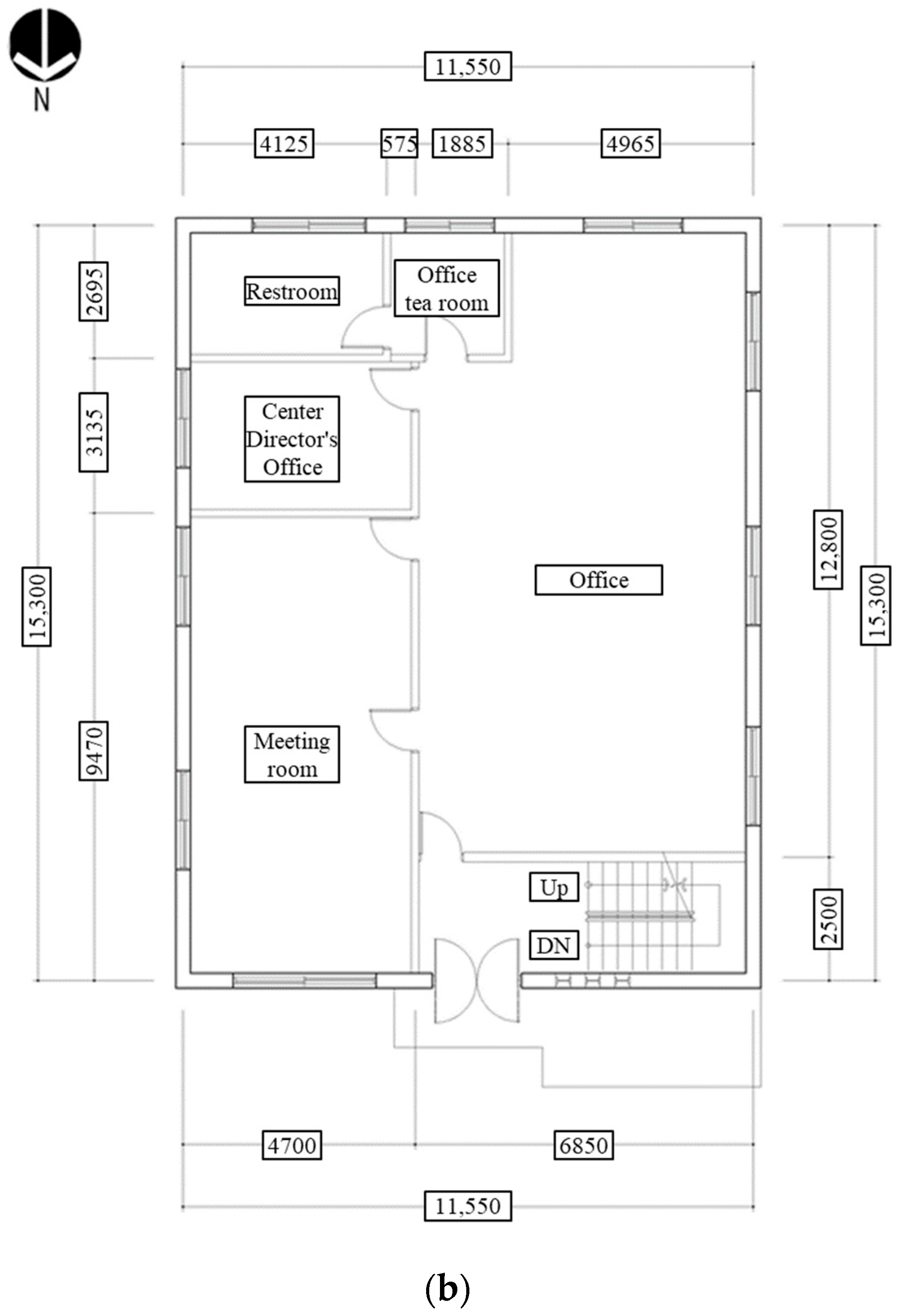
2.1. Building Description
2.2. Equipment
2.2.1. Air-Source Heat Pump
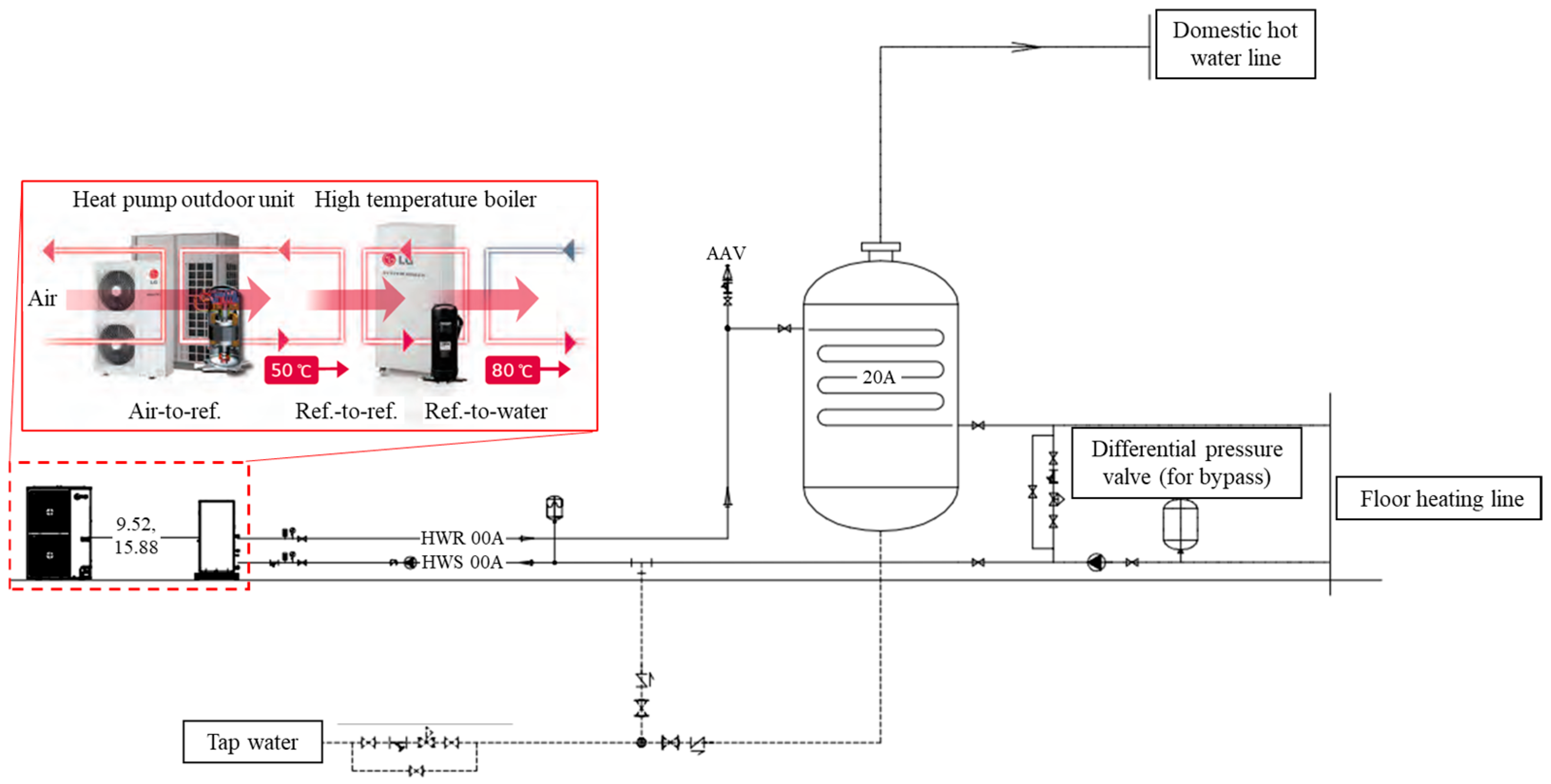
2.2.2. Boiler
2.2.3. Lights
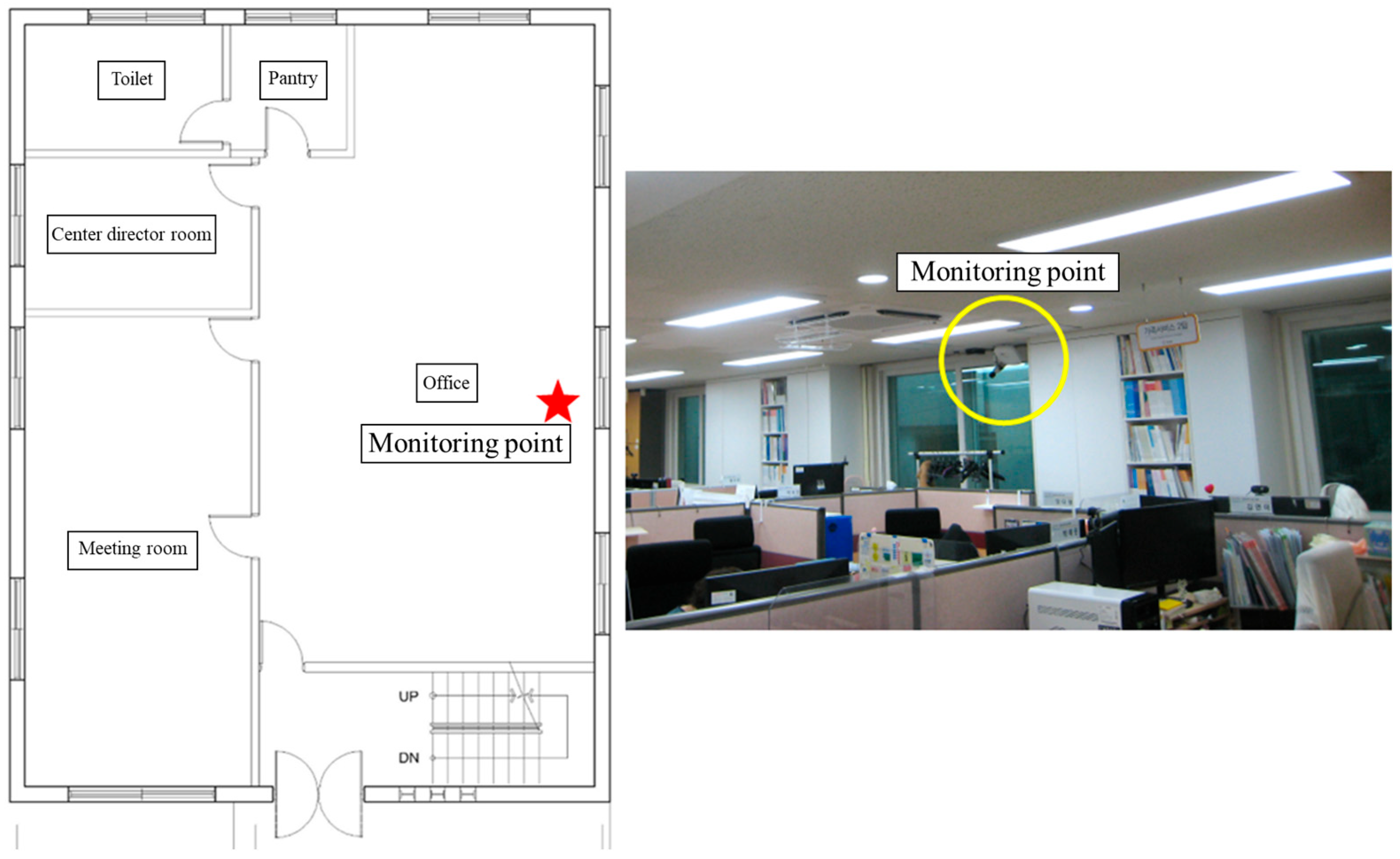
2.3. Monitoring System
3. Methodology
3.1. VRF System Modeling
3.1.1. Calibration Scenario
3.1.2. Basic Assumption
- (1)
- The total and sensible cooling capacities and power consumption were assumed to increase proportionally with indoor wet-bulb temperature, independent of dry-bulb temperature under identical wet-bulb conditions.
- (2)
- The supply airflow rate was considered constant regardless of part-load conditions.
- (3)
- Performance outputs were calculated by applying weighting factors from external performance files to rated capacities and power input. These factors depend on outdoor and indoor dry-bulb temperatures, indoor wet-bulb temperature, and airflow ratio. Detailed input data are summarized in Appendix C.
3.1.3. Calculation Procedure
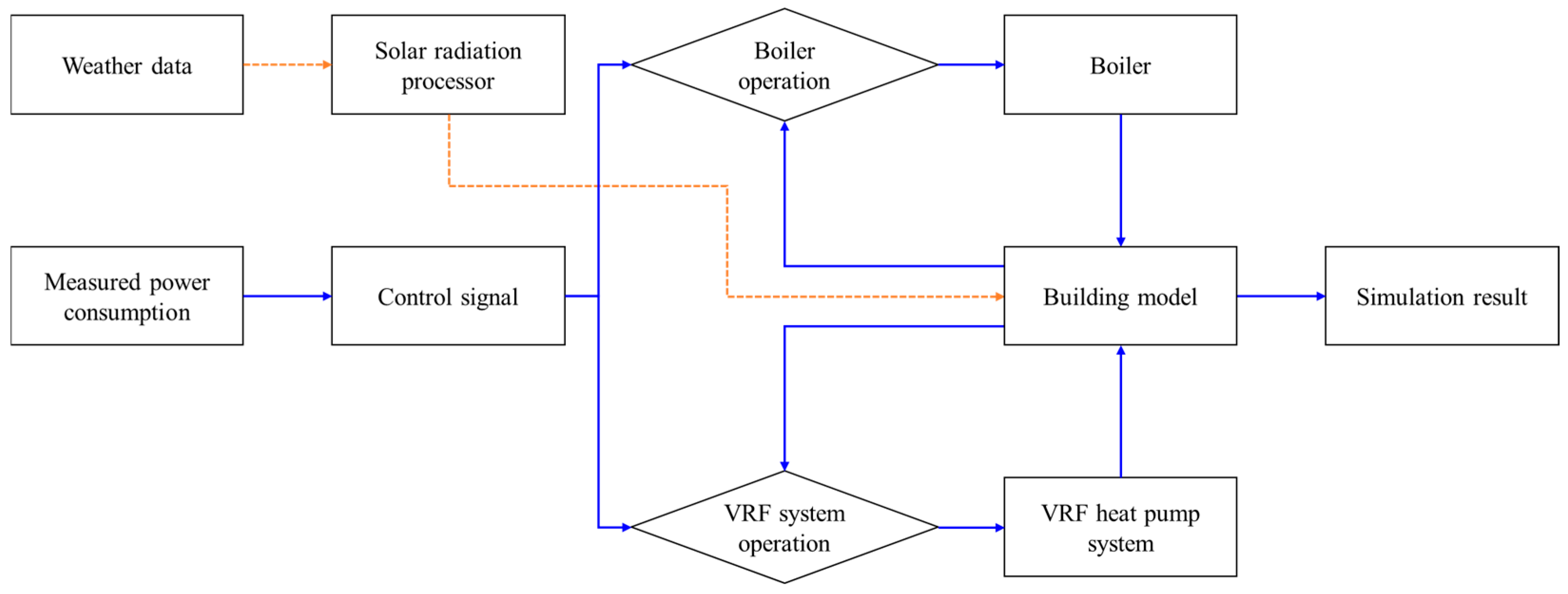
3.1.4. Control Logic and Setting
3.2. Boiler
3.3. Simulation Overview
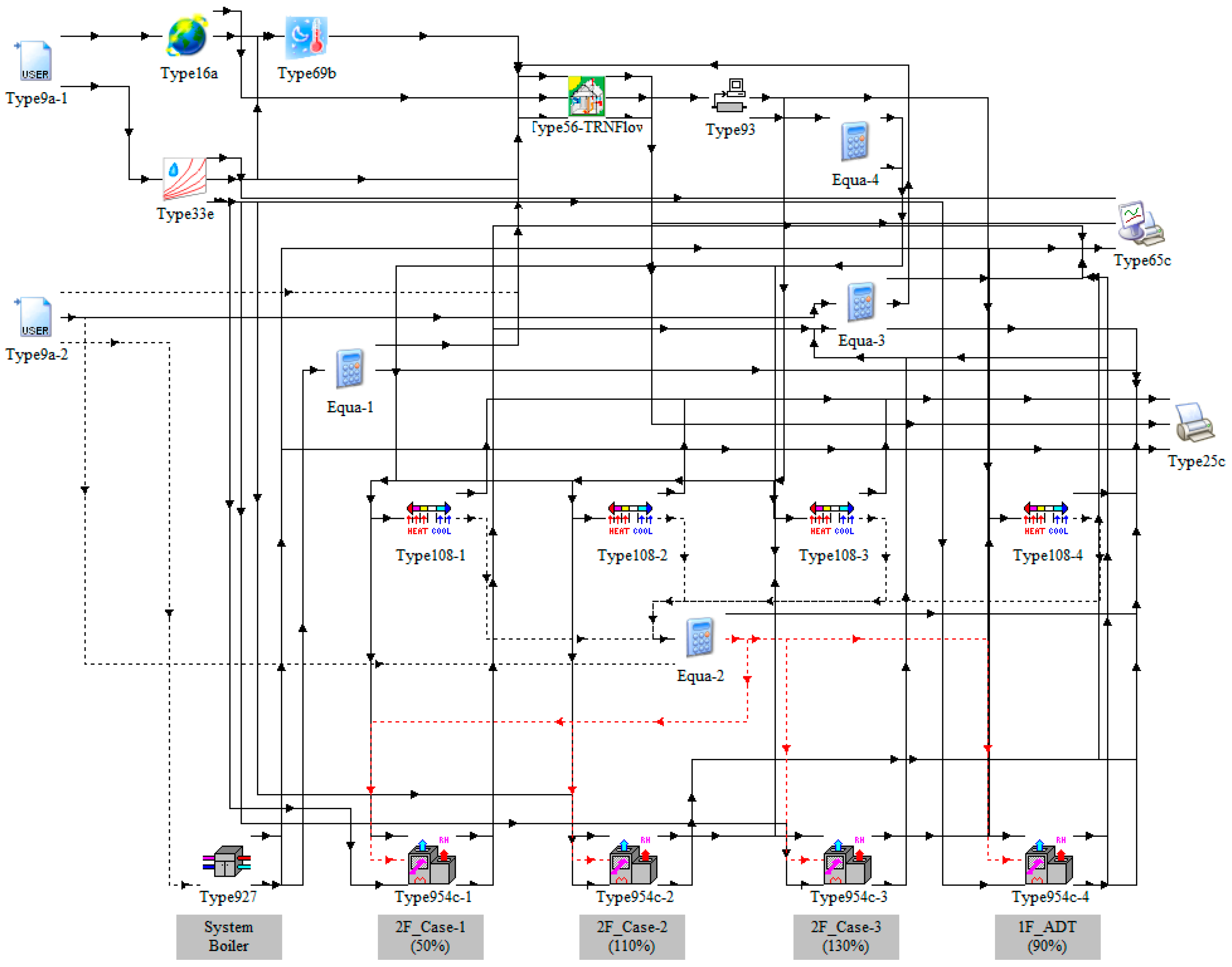
3.3.1. Simulation Studio Model
3.3.2. Weather Data
3.3.3. Building Model
3.3.4. Inner Heat Gain
3.3.5. Ventilation
3.3.6. Metrics and Criteria
4. Results
4.1. Indoor Temperature
4.2. VRF Heat Pump System
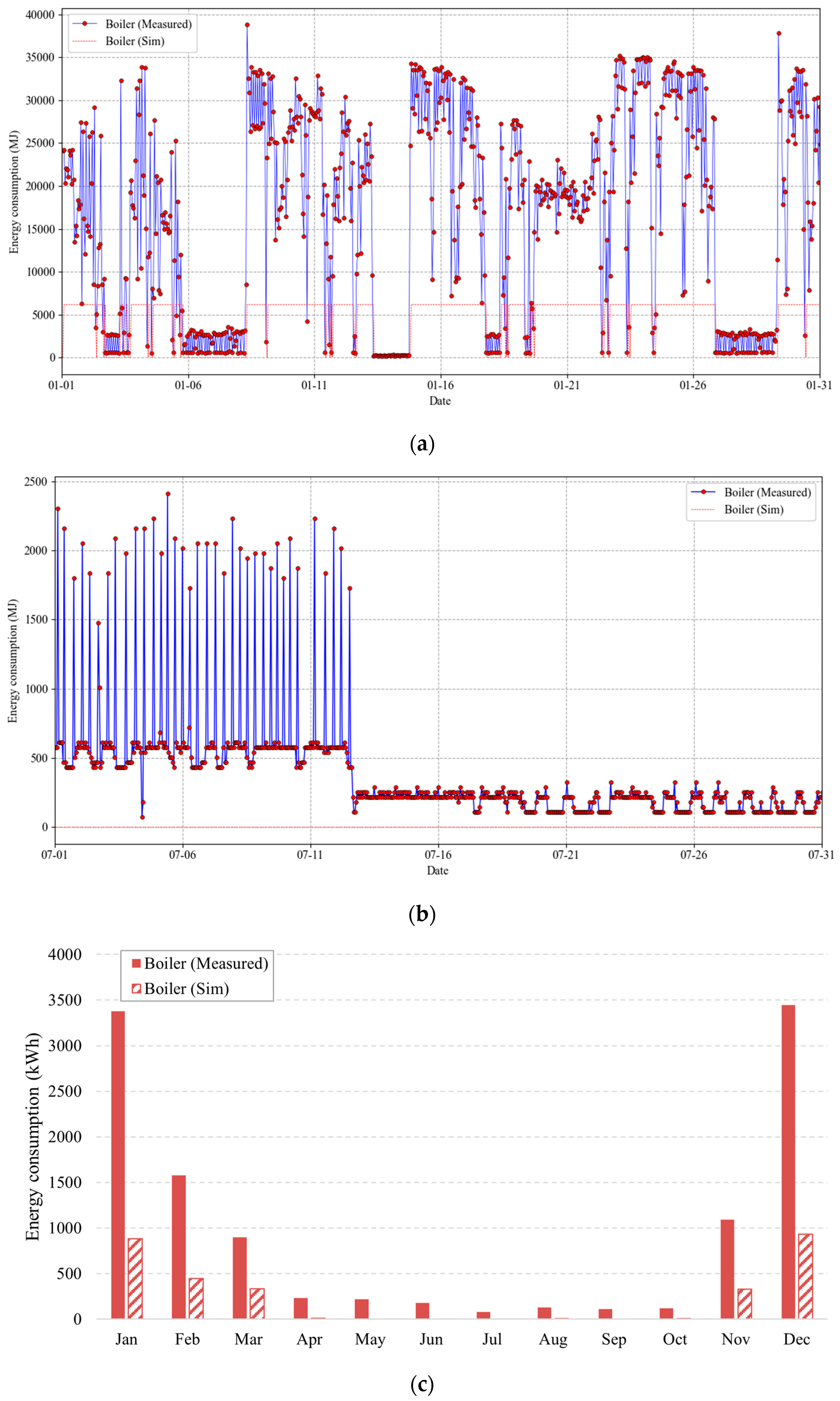
4.3. Boiler
5. Discussion
5.1. Analysis of Physical and Modeling Discrepancies
5.2. Evaluation of Practical Applicability and Limitations
5.3. Measurable Improvements and Future Research Directions
6. Conclusions
Author Contributions
Funding
Data Availability Statement
Conflicts of Interest
Abbreviations
| ASHP | Air-Source Heat Pump |
| ASOS | Automated Synoptic Observing System |
| COP | Coefficient of Performance |
| CO2 | Carbon Dioxide |
| CVRMSE | Coefficient of Variation of the Root Mean Square Error |
| EER | Energy efficiency ratio |
| HVAC | Heating, Ventilating and Air-conditioning |
| IAC | Indoor Air Conditioner |
| OAC | Outdoor Air Conditioner |
| PLR | Part Load Ratio |
| RMSE | Root Mean Square Error |
Appendix A

| Part Load Ratio | Outdoor Air Temp. | Indoor Air Temperature (°C) (Dry-Bulb/Wet-Bulb) | |||||||||||||
|---|---|---|---|---|---|---|---|---|---|---|---|---|---|---|---|
| (%) | (°C) | 20/14 | 23/16 | 26/18 | 27/19 | 28/20 | 30/22 | 32/24 | |||||||
| TC | PI | TC | PI | TC | PI | TC | PI | TC | PI | TC | PI | TC | PI | ||
| 130 | 10 | 20.5 | 3.44 | 24.4 | 4.21 | 28.3 | 5.02 | 29.4 | 5.12 | 29.7 | 5.02 | 30.5 | 4.79 | 31.2 | 4.59 |
| 12 | 20.5 | 3.05 | 24.4 | 4.29 | 28.3 | 5.1 | 29 | 5.09 | 29.5 | 4.99 | 30.1 | 4.76 | 30.8 | 4.69 | |
| 14 | 20.5 | 3.56 | 24.4 | 4.37 | 28.2 | 5.16 | 28.6 | 5.06 | 29 | 4.96 | 39.7 | 4.2 | 30.5 | 4.96 | |
| 16 | 20.5 | 3.64 | 24.4 | 4.45 | 27.9 | 5.15 | 28.2 | 5.1 | 28.6 | 5.13 | 29.3 | 5.19 | 30.1 | 5.23 | |
| 18 | 20.5 | 3.7 | 24.4 | 4.55 | 27.5 | 5.34 | 27.8 | 5.36 | 28.2 | 5.39 | 29 | 5.44 | 29.7 | 5.5 | |
| 20 | 20.5 | 3.78 | 24.4 | 4.85 | 27.1 | 5.6 | 27.5 | 5.63 | 27.8 | 5.66 | 28.6 | 5.71 | 29.3 | 5.77 | |
| 21 | 20.5 | 3.88 | 24.4 | 5.02 | 26.9 | 5.73 | 27.3 | 5.75 | 27.6 | 5.78 | 28.4 | 5.84 | 29.1 | 5.9 | |
| 23 | 20.5 | 4.17 | 24.4 | 5.39 | 26.6 | 6 | 26.9 | 6.02 | 27.3 | 6.05 | 28 | 6.11 | 28.7 | 6.18 | |
| 25 | 20.5 | 4.45 | 24.4 | 5.75 | 26.1 | 6.25 | 26.6 | 6.29 | 26.9 | 6.32 | 27.6 | 6.38 | 28.4 | 6.45 | |
| 27 | 20.5 | 4.76 | 24.4 | 6.15 | 25.8 | 6.52 | 26.1 | 6.55 | 26.6 | 6.58 | 27.3 | 6.66 | 28 | 6.72 | |
| 29 | 20.5 | 5.07 | 24.4 | 6.58 | 25.4 | 6.78 | 25.8 | 6.85 | 26.1 | 6.86 | 26.9 | 6.92 | 27.6 | 7 | |
| 31 | 20.5 | 5.41 | 24.4 | 6.97 | 25 | 7.04 | 25.4 | 7.09 | 25.8 | 7.12 | 26.5 | 7.2 | 27.2 | 7.27 | |
| 33 | 20.5 | 5.77 | 24.4 | 7.23 | 24.6 | 7.31 | 25 | 7.36 | 25.4 | 7.4 | 26.1 | 7.47 | 26.8 | 7.56 | |
| 35 | 20.5 | 6.15 | 24.4 | 7.48 | 24.2 | 7.58 | 24.6 | 7.63 | 25 | 7.67 | 25.7 | 7.75 | 26.5 | 7.84 | |
| 37 | 20.5 | 6.55 | 24.4 | 7.75 | 23.9 | 7.85 | 24.2 | 7.9 | 24.6 | 7.94 | 25.3 | 8.02 | 26.1 | 8.12 | |
| 120 | 10 | 18.9 | 3.13 | 22.5 | 3.84 | 26.2 | 4.56 | 28 | 4.93 | 29.4 | 5.15 | 30 | 4.95 | 30.7 | 4.76 |
| 12 | 18.9 | 3.19 | 22.5 | 3.91 | 26.2 | 4.65 | 28 | 5.03 | 29 | 5.12 | 29.6 | 4.92 | 30.3 | 4.72 | |
| 14 | 18.9 | 3.26 | 22.5 | 3.98 | 26.2 | 4.73 | 28 | 5.13 | 28.5 | 5.09 | 29.3 | 4.89 | 30 | 4.93 | |
| 16 | 18.9 | 3.32 | 22.5 | 4.07 | 26.2 | 4.83 | 27.9 | 5.16 | 28.2 | 5.1 | 28.9 | 5.15 | 29.5 | 5.19 | |
| 18 | 18.9 | 3.39 | 22.5 | 4.14 | 26.2 | 5 | 27.5 | 5.33 | 27.8 | 2.36 | 28.5 | 5.41 | 29.2 | 5.46 | |
| 20 | 18.9 | 3.44 | 22.5 | 4.31 | 26.2 | 5.37 | 27.1 | 5.6 | 27.5 | 2.61 | 28.1 | 5.67 | 28.8 | 5.73 | |
| 21 | 18.9 | 3.49 | 22.5 | 4.46 | 26.2 | 5.57 | 26.9 | 5.73 | 27.2 | 5.75 | 28 | 5.81 | 28.6 | 5.85 | |
| 23 | 18.9 | 3.73 | 22.5 | 4.78 | 26.2 | 5.95 | 26.5 | 5.98 | 26.9 | 6.01 | 27.5 | 6.07 | 28.2 | 6.12 | |
| 25 | 18.9 | 3.98 | 22.5 | 5.12 | 25.8 | 6.21 | 26.1 | 6.25 | 26.4 | 6.28 | 27.2 | 6.34 | 27.9 | 6.39 | |
| 27 | 18.9 | 4.25 | 22.5 | 5.47 | 25.4 | 6.48 | 25.8 | 6.51 | 26.1 | 6.55 | 26.8 | 6.61 | 27.5 | 6.66 | |
| 29 | 18.9 | 4.54 | 22.5 | 5.84 | 25 | 6.75 | 25.4 | 6.78 | 25.7 | 6.8 | 26.4 | 6.87 | 27.1 | 6.95 | |
| 31 | 18.9 | 4.83 | 22.5 | 6.24 | 24.6 | 7 | 25 | 7.03 | 25.4 | 7.07 | 26 | 7.14 | 26.7 | 7.21 | |
| 33 | 18.9 | 5.15 | 22.5 | 6.65 | 24.3 | 7.26 | 24.6 | 7.3 | 24.9 | 7.34 | 25.6 | 7.41 | 26.3 | 7.48 | |
| 35 | 18.9 | 5.47 | 22.5 | 7.09 | 23.9 | 7.54 | 24.2 | 7.57 | 24.6 | 7.61 | 25.3 | 7.68 | 25.9 | 7.77 | |
| 37 | 18.9 | 5.83 | 22.5 | 7.56 | 23.5 | 7.8 | 23.9 | 7.84 | 24.2 | 7.88 | 24.9 | 7.97 | 25.5 | 8.05 | |
| 110 | 10 | 17.3 | 2.85 | 20.7 | 3.47 | 24 | 4.12 | 25.7 | 4.46 | 27.3 | 4.81 | 29.4 | 5.1 | 30.1 | 4.92 |
| 12 | 17.3 | 2.91 | 20.7 | 3.53 | 24 | 4.21 | 25.7 | 4.55 | 27.3 | 4.89 | 29.1 | 5.07 | 29.7 | 4.89 | |
| 14 | 17.3 | 2.96 | 20.7 | 3.6 | 24 | 4.28 | 25.7 | 4.64 | 27.3 | 4.99 | 28.7 | 5.05 | 29.3 | 4.89 | |
| 16 | 17.3 | 3.02 | 20.7 | 3.67 | 24 | 4.37 | 25.7 | 4.72 | 27.3 | 5.07 | 28.3 | 5.1 | 28.9 | 5.16 | |
| 18 | 17.3 | 3.08 | 20.7 | 3.74 | 24 | 4.45 | 25.7 | 4.85 | 27.3 | 5.33 | 27.9 | 5.37 | 28.6 | 5.41 | |
| 20 | 17.3 | 3.13 | 20.7 | 3.83 | 24 | 4.72 | 25.7 | 5.22 | 26.9 | 5.58 | 27.6 | 5.64 | 28.2 | 5.68 | |
| 21 | 17.3 | 3.16 | 20.7 | 3.94 | 24 | 4.89 | 25.7 | 5.4 | 26.7 | 5.71 | 27.3 | 5.75 | 28 | 5.81 | |
| 23 | 17.3 | 3.3 | 20.7 | 4.22 | 24 | 5.24 | 25.7 | 5.8 | 26.3 | 5.98 | 27 | 6.02 | 27.6 | 6.08 | |
| 25 | 17.3 | 3.53 | 20.7 | 4.51 | 24 | 5.61 | 25.7 | 6.21 | 26 | 6.24 | 26.6 | 6.29 | 27.2 | 6.35 | |
| 27 | 17.3 | 3.77 | 20.7 | 4.82 | 24 | 6.01 | 25.2 | 6.46 | 25.6 | 6.49 | 26.2 | 6.55 | 26.8 | 6.61 | |
| 29 | 17.3 | 4.03 | 20.7 | 5.15 | 24 | 6.41 | 24.9 | 6.73 | 25.2 | 6.76 | 25.8 | 6.83 | 26.5 | 6.89 | |
| 31 | 17.3 | 4.28 | 20.7 | 5.49 | 24 | 6.85 | 24.5 | 7 | 24.8 | 7.03 | 25.5 | 7.09 | 26.1 | 7.16 | |
| 33 | 17.3 | 4.56 | 20.7 | 5.84 | 23.8 | 7.23 | 24.2 | 7.26 | 24.5 | 7.29 | 25.1 | 7.36 | 25.7 | 7.43 | |
| 35 | 17.3 | 4.85 | 20.7 | 6.24 | 23.4 | 7.49 | 23.7 | 7.51 | 24.1 | 7.56 | 24.7 | 7.63 | 25.3 | 7.71 | |
| 37 | 17.3 | 5.16 | 20.7 | 6.63 | 23.1 | 7.74 | 23.4 | 7.78 | 23.7 | 7.82 | 24.3 | 7.91 | 24.9 | 7.98 | |
| 100 | 10 | 15.1 | 2.57 | 18 | 3.12 | 21 | 3.7 | 22.4 | 4 | 23.8 | 4.29 | 26.8 | 4.9 | 29.4 | 5.07 |
| 12 | 15.1 | 2.62 | 18 | 3.18 | 21 | 3.77 | 22.4 | 4.07 | 23.8 | 4.38 | 26.8 | 5 | 29 | 5.06 | |
| 14 | 15.1 | 2.66 | 18 | 3.23 | 21 | 3.84 | 22.4 | 4.15 | 23.8 | 4.46 | 26.8 | 5.1 | 28.7 | 5.03 | |
| 16 | 15.1 | 2.71 | 18 | 3.3 | 21 | 3.91 | 22.4 | 4.22 | 23.8 | 4.55 | 26.8 | 5.16 | 28.3 | 5.12 | |
| 18 | 15.1 | 2.76 | 18 | 3.36 | 21 | 4 | 22.4 | 4.31 | 23.8 | 4.65 | 26.8 | 5.33 | 27.9 | 5.37 | |
| 20 | 15.1 | 2.82 | 18 | 3.43 | 21 | 4.11 | 22.4 | 4.54 | 23.8 | 4.98 | 26.8 | 5.58 | 27.5 | 5.64 | |
| 21 | 15.1 | 2.85 | 18 | 3.46 | 21 | 4.25 | 22.4 | 4.69 | 23.8 | 5.16 | 26.8 | 5.73 | 27.4 | 5.77 | |
| 23 | 15.1 | 2.92 | 18 | 3.7 | 21 | 4.56 | 22.4 | 5.03 | 23.8 | 5.53 | 26.8 | 5.98 | 27.4 | 6.04 | |
| 25 | 15.1 | 3.1 | 18 | 3.94 | 21 | 4.88 | 22.4 | 5.39 | 23.8 | 5.91 | 26.8 | 6.24 | 26.6 | 6.29 | |
| 27 | 15.1 | 3.32 | 18 | 4.21 | 21 | 5.22 | 22.4 | 5.75 | 23.8 | 6.32 | 26.8 | 6.51 | 26.2 | 6.56 | |
| 29 | 15.1 | 3.53 | 18 | 4.49 | 21 | 5.57 | 22.4 | 6.15 | 23.8 | 6.72 | 26.8 | 6.78 | 25.8 | 6.83 | |
| 31 | 15.1 | 3.77 | 18 | 4.79 | 21 | 5.94 | 22.4 | 6.56 | 23.8 | 6.97 | 26.8 | 7.03 | 25.4 | 7.09 | |
| 33 | 15.1 | 4 | 18 | 5.1 | 21 | 6.34 | 22.4 | 7 | 23.8 | 7.24 | 26.8 | 7.3 | 25 | 7.37 | |
| 35 | 15.1 | 4.25 | 18 | 5.43 | 21 | 6.75 | 22.4 | 7.47 | 23.8 | 7.5 | 26.8 | 7.57 | 24.6 | 7.63 | |
| 37 | 15.1 | 4.52 | 18 | 5.78 | 21 | 7.2 | 22.4 | 7.74 | 23.8 | 7.77 | 26.8 | 7.84 | 24.3 | 7.91 | |
| 90 | 10 | 13.6 | 2.31 | 16.2 | 2.78 | 18.9 | 3.27 | 20.2 | 3.53 | 21.4 | 3.8 | 24.1 | 4.35 | 26.7 | 4.9 |
| 12 | 13.6 | 2.34 | 16.2 | 2.82 | 18.9 | 3.33 | 20.2 | 3.6 | 21.4 | 3.88 | 24.1 | 4.42 | 26.7 | 4.99 | |
| 14 | 13.6 | 2.38 | 16.2 | 2.88 | 18.9 | 3.4 | 20.2 | 3.67 | 21.4 | 3.95 | 24.1 | 4.51 | 26.7 | 5.09 | |
| 16 | 13.6 | 2.42 | 16.2 | 2.93 | 18.9 | 3.47 | 20.2 | 3.74 | 21.4 | 4.03 | 24.1 | 4.61 | 26.7 | 5.17 | |
| 18 | 13.6 | 2.47 | 16.2 | 2.99 | 18.9 | 3.53 | 20.2 | 3.83 | 21.4 | 4.11 | 24.1 | 4.69 | 26.7 | 5.33 | |
| 20 | 13.6 | 2.51 | 16.2 | 3.05 | 18.9 | 3.6 | 20.2 | 3.9 | 21.4 | 4.27 | 24.1 | 5.05 | 26.7 | 5.58 | |
| 21 | 13.6 | 2.54 | 16.2 | 3.08 | 18.9 | 3.67 | 20.2 | 4.03 | 21.4 | 4.42 | 24.1 | 5.23 | 26.7 | 5.73 | |
| 23 | 13.6 | 2.59 | 16.2 | 3.2 | 18.9 | 3.93 | 20.2 | 4.32 | 21.4 | 4.73 | 24.1 | 5.61 | 26.4 | 5.98 | |
| 25 | 13.6 | 2.72 | 16.2 | 3.42 | 18.9 | 4.2 | 20.2 | 4.62 | 21.4 | 5.06 | 24.1 | 6.01 | 26 | 6.24 | |
| 27 | 13.6 | 2.91 | 16.2 | 3.64 | 18.9 | 4.48 | 20.2 | 4.93 | 21.4 | 5.41 | 24.1 | 6.42 | 25.7 | 6.51 | |
| 29 | 13.6 | 3.08 | 16.2 | 3.88 | 18.9 | 4.79 | 20.2 | 5.27 | 21.4 | 5.78 | 24.1 | 6.72 | 25.3 | 6.78 | |
| 31 | 13.6 | 3.27 | 16.2 | 4.14 | 18.9 | 5.1 | 20.2 | 5.61 | 21.4 | 6.17 | 24.1 | 6.97 | 24.9 | 7.03 | |
| 33 | 13.6 | 3.49 | 16.2 | 4.41 | 18.9 | 5.44 | 20.2 | 5.98 | 21.4 | 6.58 | 24.1 | 7.24 | 24.5 | 7.3 | |
| 35 | 13.6 | 3.7 | 16.2 | 4.68 | 18.9 | 5.78 | 20.2 | 6.38 | 21.4 | 7 | 23.6 | 7.51 | 24.1 | 7.57 | |
| 37 | 13.6 | 3.93 | 16.2 | 4.98 | 18.9 | 6.15 | 20.2 | 6.8 | 21.4 | 7.47 | 23.3 | 7.77 | 23.8 | 7.84 | |
| 80 | 10 | 12.1 | 2.04 | 14.4 | 2.45 | 16.7 | 2.88 | 17.9 | 3.1 | 19.1 | 3.33 | 21.4 | 3.8 | 23.8 | 4.28 |
| 12 | 12.1 | 2.08 | 14.4 | 2.48 | 16.7 | 2.93 | 17.9 | 3.16 | 19.1 | 3.39 | 21.4 | 3.87 | 23.8 | 4.37 | |
| 14 | 12.1 | 2.11 | 14.4 | 2.54 | 16.7 | 2.98 | 17.9 | 3.22 | 19.1 | 3.44 | 21.4 | 3.94 | 23.8 | 4.44 | |
| 16 | 12.1 | 2.14 | 14.4 | 2.58 | 16.7 | 3.03 | 17.9 | 3.27 | 19.1 | 3.52 | 21.4 | 4.03 | 23.8 | 4.54 | |
| 18 | 12.1 | 2.18 | 14.4 | 2.62 | 16.7 | 3.09 | 17.9 | 3.33 | 19.1 | 3.59 | 21.4 | 4.1 | 23.8 | 4.62 | |
| 20 | 12.1 | 2.23 | 14.4 | 2.68 | 16.7 | 3.16 | 17.9 | 3.4 | 19.1 | 3.66 | 21.4 | 4.25 | 23.8 | 4.93 | |
| 21 | 12.1 | 2.24 | 14.4 | 2.71 | 16.7 | 3.19 | 17.9 | 3.44 | 19.1 | 3.74 | 21.4 | 4.39 | 23.8 | 5.12 | |
| 23 | 12.1 | 2.28 | 14.4 | 2.75 | 16.7 | 3.33 | 17.9 | 3.66 | 19.1 | 4 | 21.4 | 4.71 | 23.8 | 5.49 | |
| 25 | 12.1 | 2.37 | 14.4 | 2.93 | 16.7 | 3.57 | 17.9 | 3.91 | 19.1 | 4.28 | 21.4 | 5.05 | 23.8 | 5.87 | |
| 27 | 12.1 | 2.51 | 14.4 | 3.12 | 16.7 | 3.81 | 17.9 | 4.18 | 19.1 | 4.56 | 21.4 | 5.39 | 23.8 | 6.28 | |
| 29 | 12.1 | 2.66 | 14.4 | 3.33 | 16.7 | 4.05 | 17.9 | 4.45 | 19.1 | 4.88 | 21.4 | 5.75 | 23.8 | 6.72 | |
| 31 | 12.1 | 2.83 | 14.4 | 3.35 | 16.7 | 4.32 | 17.9 | 4.75 | 19.1 | 5.19 | 21.4 | 6.14 | 23.8 | 6.97 | |
| 33 | 12.1 | 3.01 | 14.4 | 3.77 | 16.7 | 4.61 | 17.9 | 5.06 | 19.1 | 5.53 | 21.4 | 6.55 | 23.8 | 7.23 | |
| 35 | 12.1 | 3.19 | 14.4 | 4 | 16.7 | 4.9 | 17.9 | 5.39 | 19.1 | 5.9 | 21.4 | 6.97 | 23.6 | 7.5 | |
| 37 | 12.1 | 3.37 | 14.4 | 4.25 | 16.7 | 5.2 | 17.9 | 5.73 | 19.1 | 6.27 | 21.4 | 7.44 | 23.2 | 7.77 | |
| 70 | 10 | 10.6 | 1.8 | 12.6 | 2.14 | 14.7 | 2.48 | 15.7 | 2.68 | 16.7 | 2.86 | 18.7 | 3.26 | 20.8 | 3.67 |
| 12 | 10.6 | 1.83 | 12.6 | 2.17 | 14.6 | 2.54 | 15.7 | 2.72 | 16.7 | 2.92 | 18.7 | 3.32 | 20.8 | 3.74 | |
| 14 | 10.6 | 1.86 | 12.6 | 2.2 | 14.6 | 2.58 | 15.7 | 2.76 | 16.7 | 2.96 | 18.7 | 3.39 | 20.8 | 3.8 | |
| 16 | 10.6 | 1.89 | 12.6 | 2.24 | 14.6 | 2.62 | 15.7 | 2.82 | 16.7 | 3.02 | 18.7 | 3.44 | 20.8 | 3.88 | |
| 18 | 10.6 | 1.91 | 12.6 | 2.28 | 14.6 | 2.68 | 15.7 | 2.88 | 16.7 | 3.08 | 18.7 | 3.5 | 20.8 | 3.95 | |
| 20 | 10.6 | 1.94 | 12.6 | 2.32 | 14.6 | 2.72 | 15.7 | 2.93 | 16.7 | 3.15 | 18.7 | 3.59 | 20.8 | 4.07 | |
| 21 | 10.6 | 1.97 | 12.6 | 2.34 | 14.6 | 2.75 | 15.7 | 2.96 | 16.7 | 3.18 | 18.7 | 3.64 | 20.8 | 4.21 | |
| 23 | 10.6 | 2 | 12.6 | 2.4 | 14.6 | 2.81 | 15.7 | 3.06 | 16.7 | 3.33 | 18.7 | 3.9 | 20.8 | 4.51 | |
| 25 | 10.6 | 2.03 | 12.6 | 2.48 | 14.6 | 2.99 | 15.7 | 3.27 | 16.7 | 3.56 | 18.7 | 4.17 | 20.8 | 4.82 | |
| 27 | 10.6 | 2.14 | 12.6 | 2.65 | 14.6 | 3.19 | 15.7 | 3.47 | 16.7 | 3.8 | 18.7 | 4.45 | 20.8 | 5.16 | |
| 29 | 10.6 | 2.28 | 12.6 | 2.81 | 14.6 | 3.39 | 15.7 | 3.7 | 16.7 | 4.04 | 18.7 | 4.75 | 20.8 | 5.5 | |
| 31 | 10.6 | 2.42 | 12.6 | 2.99 | 14.6 | 3.61 | 15.7 | 3.95 | 16.7 | 4.31 | 18.7 | 5.06 | 20.8 | 5.87 | |
| 33 | 10.6 | 2.57 | 12.6 | 3.16 | 14.6 | 3.84 | 15.7 | 4.2 | 16.7 | 4.58 | 18.7 | 5.39 | 20.8 | 6.27 | |
| 35 | 10.6 | 2.71 | 12.6 | 3.36 | 14.6 | 4.08 | 15.7 | 4.46 | 16.7 | 4.88 | 18.7 | 5.74 | 20.8 | 6.68 | |
| 37 | 10.6 | 2.88 | 12.6 | 3.56 | 14.6 | 4.34 | 15.7 | 4.75 | 16.7 | 5.19 | 18.7 | 6.11 | 20.8 | 7.12 | |
| 60 | 10 | 9 | 1.56 | 10.8 | 1.83 | 12.6 | 2.13 | 13.4 | 2.28 | 14.3 | 2.42 | 16.1 | 2.75 | 17.8 | 3.08 |
| 12 | 9 | 1.59 | 10.8 | 1.86 | 12.6 | 2.15 | 13.4 | 2.31 | 14.3 | 2.47 | 16.1 | 2.79 | 17.8 | 3.13 | |
| 14 | 9 | 1.6 | 10.8 | 1.89 | 12.6 | 2.2 | 13.4 | 2.35 | 14.3 | 2.51 | 16.1 | 2.85 | 17.8 | 3.19 | |
| 16 | 9 | 1.63 | 10.8 | 1.93 | 12.6 | 2.23 | 13.4 | 2.4 | 14.3 | 2.57 | 16.1 | 2.91 | 17.8 | 3.25 | |
| 18 | 9 | 1.66 | 10.8 | 1.96 | 12.6 | 2.27 | 13.4 | 2.44 | 14.3 | 2.61 | 16.1 | 2.95 | 17.8 | 3.32 | |
| 20 | 9 | 1.69 | 10.8 | 1.98 | 12.6 | 2.31 | 13.4 | 2.48 | 14.3 | 2.65 | 16.1 | 3.01 | 17.8 | 3.39 | |
| 21 | 9 | 1.7 | 10.8 | 2 | 12.6 | 2.34 | 13.4 | 2.51 | 14.3 | 2.68 | 16.1 | 3.05 | 17.8 | 3.42 | |
| 23 | 9 | 1.73 | 10.8 | 2.04 | 12.6 | 2.37 | 13.4 | 2.55 | 14.3 | 2.74 | 16.1 | 3.16 | 17.8 | 3.63 | |
| 25 | 9 | 1.76 | 10.8 | 2.08 | 12.6 | 2.47 | 13.4 | 2.68 | 14.3 | 2.91 | 16.1 | 3.37 | 17.8 | 3.88 | |
| 27 | 9 | 1.81 | 10.8 | 2.2 | 12.6 | 2.62 | 13.4 | 2.85 | 14.3 | 3.09 | 16.1 | 3.59 | 17.8 | 4.14 | |
| 29 | 9 | 1.93 | 10.8 | 2.34 | 12.6 | 2.79 | 13.4 | 3.03 | 14.3 | 3.29 | 16.1 | 3.83 | 17.8 | 4.42 | |
| 31 | 9 | 2.04 | 10.8 | 2.48 | 12.6 | 2.96 | 13.4 | 3.23 | 14.3 | 3.5 | 16.1 | 4.08 | 17.8 | 4.71 | |
| 33 | 9 | 2.15 | 10.8 | 2.62 | 12.6 | 3.15 | 13.4 | 3.43 | 14.3 | 3.73 | 16.1 | 4.34 | 17.8 | 5.02 | |
| 35 | 9 | 2.28 | 10.8 | 2.79 | 12.6 | 3.35 | 13.4 | 3.64 | 14.3 | 3.95 | 16.1 | 4.62 | 17.8 | 5.33 | |
| 37 | 9 | 2.41 | 10.8 | 2.95 | 12.6 | 3.54 | 13.4 | 3.87 | 14.3 | 4.2 | 16.1 | 4.9 | 17.8 | 5.67 | |
| 50 | 10 | 7.6 | 1.35 | 9 | 1.56 | 10.5 | 1.77 | 11.2 | 1.9 | 11.9 | 2.01 | 13.4 | 2.27 | 14.9 | 2.52 |
| 12 | 7.6 | 1.36 | 9 | 1.57 | 10.5 | 1.8 | 11.2 | 1.93 | 11.9 | 2.06 | 13.4 | 2.31 | 14.9 | 2.57 | |
| 14 | 7.6 | 1.37 | 9 | 1.6 | 10.5 | 1.83 | 11.2 | 1.96 | 11.9 | 2.08 | 13.4 | 2.34 | 14.9 | 2.61 | |
| 16 | 7.6 | 1.4 | 9 | 1.63 | 10.5 | 1.86 | 11.2 | 2 | 11.9 | 2.11 | 13.4 | 2.38 | 14.9 | 2.65 | |
| 18 | 7.6 | 1.42 | 9 | 1.64 | 10.5 | 1.89 | 11.2 | 2.03 | 11.9 | 2.15 | 13.4 | 2.42 | 14.9 | 2.71 | |
| 20 | 7.6 | 1.43 | 9 | 1.67 | 10.5 | 1.93 | 11.2 | 2.06 | 11.9 | 2.2 | 13.4 | 2.47 | 14.9 | 2.76 | |
| 21 | 7.6 | 1.45 | 9 | 1.69 | 10.5 | 1.94 | 11.2 | 2.08 | 11.9 | 2.21 | 13.4 | 2.49 | 14.9 | 2.79 | |
| 23 | 7.6 | 1.47 | 9 | 1.72 | 10.5 | 1.97 | 11.2 | 2.11 | 11.9 | 2.25 | 13.4 | 2.54 | 14.9 | 2.85 | |
| 25 | 7.6 | 1.49 | 9 | 1.74 | 10.5 | 2.01 | 11.2 | 2.15 | 11.9 | 2.32 | 13.4 | 2.66 | 14.9 | 3.05 | |
| 27 | 7.6 | 1.52 | 9 | 1.8 | 10.5 | 2.13 | 11.2 | 2.3 | 11.9 | 2.47 | 13.4 | 2.85 | 14.9 | 3.25 | |
| 29 | 7.6 | 1.6 | 9 | 1.91 | 10.5 | 2.25 | 11.2 | 2.44 | 11.9 | 2.62 | 13.4 | 3.02 | 14.9 | 3.44 | |
| 31 | 7.6 | 1.69 | 9 | 2.03 | 10.5 | 2.4 | 11.2 | 2.58 | 11.9 | 2.79 | 13.4 | 3.22 | 14.9 | 3.67 | |
| 33 | 7.6 | 1.79 | 9 | 2.14 | 10.5 | 2.54 | 11.2 | 2.74 | 11.9 | 2.96 | 13.4 | 3.42 | 14.9 | 3.91 | |
| 35 | 7.6 | 1.89 | 9 | 2.27 | 10.5 | 2.68 | 11.2 | 2.91 | 11.9 | 3.13 | 13.4 | 3.61 | 14.9 | 4.15 | |
| 37 | 7.6 | 2 | 9 | 2.4 | 10.5 | 2.83 | 11.2 | 3.08 | 11.9 | 3.32 | 13.4 | 3.86 | 14.9 | 4.41 | |
| Part Load Ratio | Outdoor Air Temp. | Indoor Air Temperature (°C) (Dry-Bulb/Wet-Bulb) | |||||||||||||
|---|---|---|---|---|---|---|---|---|---|---|---|---|---|---|---|
| (%) | (°C) | 20/14 | 23/16 | 26/18 | 27/19 | 28/20 | 30/22 | 32/24 | |||||||
| TC | PI | TC | PI | TC | PI | TC | PI | TC | PI | TC | PI | TC | PI | ||
| 130 | 10 | 25.6 | 4.611 | 30.5 | 5.636 | 35.4 | 6.72 | 36.7 | 6.85 | 37.2 | 6.72 | 38.1 | 6.414 | 39 | 6.148 |
| 12 | 25.6 | 4.687 | 30.5 | 5.75 | 35.4 | 6.83 | 36.2 | 6.812 | 36.8 | 6.679 | 37.6 | 6.376 | 38.5 | 6.281 | |
| 14 | 25.6 | 4.763 | 30.5 | 5.844 | 35.3 | 6.907 | 35.8 | 6.774 | 36.2 | 6.641 | 37.2 | 6.58 | 38.1 | 6.641 | |
| 16 | 25.6 | 4.877 | 30.5 | 5.958 | 34.9 | 6.888 | 35.3 | 6.83 | 35.7 | 6.869 | 36.6 | 6.95 | 37.6 | 7.002 | |
| 18 | 25.6 | 4.95 | 30.5 | 6.091 | 34.3 | 7.154 | 34.8 | 7.17 | 35.3 | 7.211 | 36.2 | 7.287 | 37.2 | 7.36 | |
| 20 | 25.6 | 5.066 | 30.5 | 6.49 | 33.8 | 7.5 | 34.4 | 7.533 | 34.8 | 7.571 | 35.7 | 7.65 | 36.6 | 7.723 | |
| 21 | 25.6 | 5.199 | 30.5 | 6.72 | 33.6 | 7.666 | 34.1 | 7.704 | 34.6 | 7.74 | 35.5 | 7.82 | 36.4 | 7.89 | |
| 23 | 25.6 | 5.579 | 30.5 | 7.211 | 33.2 | 8.03 | 33.6 | 8.065 | 34.1 | 8.1 | 35 | 8.18 | 35.9 | 8.273 | |
| 25 | 25.6 | 5.958 | 30.5 | 7.704 | 32.7 | 8.368 | 33.2 | 8.425 | 33.6 | 8.46 | 34.6 | 8.54 | 35.5 | 8.634 | |
| 27 | 25.6 | 6.376 | 30.5 | 8.235 | 32.3 | 8.729 | 32.7 | 8.767 | 33.2 | 8.81 | 34.1 | 8.918 | 35 | 8.994 | |
| 29 | 25.6 | 6.793 | 30.5 | 8.81 | 31.7 | 9.07 | 32.2 | 9.127 | 32.7 | 9.184 | 33.6 | 9.26 | 34.6 | 9.37 | |
| 31 | 25.6 | 7.249 | 30.4 | 9.336 | 31.2 | 9.431 | 31.7 | 9.49 | 32.2 | 9.526 | 33.1 | 9.64 | 34 | 9.734 | |
| 33 | 25.6 | 7.723 | 29.9 | 9.677 | 30.8 | 9.791 | 31.3 | 9.848 | 31.7 | 9.91 | 32.7 | 10 | 33.5 | 10.114 | |
| 35 | 25.6 | 8.235 | 29.3 | 10.019 | 30.3 | 10.152 | 30.8 | 10.209 | 31.3 | 10.266 | 32.2 | 10.38 | 33.1 | 10.493 | |
| 37 | 25.6 | 8.767 | 28.9 | 10.38 | 29.9 | 10.512 | 30.3 | 10.57 | 30.8 | 10.626 | 31.6 | 10.74 | 32.6 | 10.87 | |
| 120 | 10 | 23.7 | 4.194 | 28.2 | 5.142 | 32.7 | 6.11 | 35 | 6.603 | 36.7 | 6.888 | 37.5 | 6.622 | 38.4 | 6.376 |
| 12 | 23.7 | 4.269 | 28.2 | 5.237 | 32.7 | 6.224 | 35 | 6.736 | 36.2 | 6.85 | 37 | 6.584 | 37.9 | 6.319 | |
| 14 | 23.7 | 4.364 | 28.2 | 5.33 | 32.7 | 6.338 | 35 | 6.869 | 35.7 | 6.812 | 36.6 | 6.546 | 37.4 | 6.603 | |
| 16 | 23.7 | 4.44 | 28.2 | 5.446 | 32.7 | 6.471 | 34.8 | 6.907 | 35.3 | 6.83 | 36.1 | 6.888 | 36.9 | 6.95 | |
| 18 | 23.7 | 4.535 | 28.2 | 5.541 | 32.7 | 6.7 | 34.3 | 7.135 | 34.7 | 7.17 | 35.6 | 7.249 | 36.5 | 7.306 | |
| 20 | 23.7 | 4.611 | 28.2 | 5.769 | 32.7 | 7.192 | 33.9 | 7.5 | 343 | 7.514 | 35.1 | 7.59 | 36 | 7.666 | |
| 21 | 23.7 | 4.668 | 28.2 | 5.977 | 32.7 | 7.457 | 33.6 | 7.666 | 34 | 7.704 | 34.9 | 7.78 | 35.8 | 7.837 | |
| 23 | 23.7 | 4.991 | 28.2 | 6.395 | 32.7 | 7.97 | 33.2 | 8.008 | 33.6 | 8.046 | 34.4 | 8.121 | 35.3 | 8.197 | |
| 25 | 23.7 | 5.33 | 28.2 | 6.85 | 32.7 | 8.311 | 32.6 | 8.368 | 33.1 | 8.406 | 34 | 8.482 | 34.8 | 8.56 | |
| 27 | 23.7 | 5.693 | 28.2 | 7.324 | 31.8 | 8.672 | 32.2 | 8.71 | 32.6 | 8.767 | 33.5 | 8.843 | 34.3 | 8.918 | |
| 29 | 23.7 | 6.072 | 28.2 | 7.818 | 31.3 | 9.03 | 31.7 | 9.07 | 32.1 | 9.11 | 33 | 9.203 | 33.9 | 9.298 | |
| 31 | 23.7 | 6.47 | 28.2 | 8.349 | 30.8 | 9.37 | 31.3 | 9.412 | 31.7 | 9.469 | 32.5 | 9.564 | 33.4 | 9.658 | |
| 33 | 23.7 | 6.888 | 28.2 | 8.899 | 30.4 | 9.72 | 30.8 | 9.77 | 31.2 | 9.829 | 32 | 9.924 | 32.9 | 10.019 | |
| 35 | 23.7 | 7.324 | 28.2 | 9.49 | 29.8 | 10.095 | 30.2 | 10.133 | 30.8 | 10.19 | 31.6 | 10.285 | 32.4 | 10.398 | |
| 37 | 23.7 | 7.799 | 28.2 | 10.114 | 29.4 | 10.44 | 29.8 | 10.493 | 30.2 | 10.55 | 31.1 | 10.664 | 31.9 | 10.778 | |
| 110 | 10 | 21.7 | 3.814 | 25.8 | 4.649 | 30 | 5.522 | 32.1 | 5.977 | 34.2 | 6.433 | 36.8 | 6.83 | 37.6 | 6.584 |
| 12 | 21.7 | 3.89 | 25.8 | 4.725 | 30 | 5.636 | 32.1 | 6.091 | 34.2 | 6.546 | 36.4 | 6.793 | 37.1 | 6.546 | |
| 14 | 21.7 | 3.966 | 25.8 | 4.82 | 30 | 5.731 | 32.1 | 6.205 | 34.2 | 6.679 | 35.8 | 6.755 | 36.7 | 6.546 | |
| 16 | 21.7 | 4.042 | 25.8 | 4.915 | 30 | 5.844 | 32.1 | 6.319 | 34.2 | 6.793 | 35.4 | 6.83 | 36.1 | 6.907 | |
| 18 | 21.7 | 4.118 | 25.8 | 5.009 | 30 | 5.958 | 32.1 | 6.49 | 34.2 | 7.135 | 34.9 | 7.192 | 35.7 | 7.249 | |
| 20 | 21.7 | 4.194 | 25.8 | 5.123 | 30 | 6.319 | 32.1 | 6.983 | 33.6 | 7.476 | 34.5 | 7.552 | 35.2 | 7.609 | |
| 21 | 21.7 | 4.231 | 25.8 | 5.275 | 30 | 6.546 | 32.1 | 7.23 | 33.4 | 7.65 | 34.2 | 7.704 | 35 | 7.78 | |
| 23 | 21.7 | 4.42 | 25.8 | 5.655 | 30 | 7.021 | 32.1 | 7.76 | 32.9 | 8.008 | 33.7 | 8.065 | 34.5 | 8.14 | |
| 25 | 21.7 | 4.725 | 25.8 | 6.034 | 30 | 7.514 | 32.1 | 8.311 | 32.5 | 8.349 | 33.2 | 8.425 | 34.1 | 8.501 | |
| 27 | 21.7 | 5.047 | 25.8 | 6.452 | 30 | 8.046 | 31.6 | 8.653 | 32 | 8.691 | 32.8 | 8.767 | 33.5 | 8.843 | |
| 29 | 21.7 | 5.389 | 25.8 | 6.888 | 30 | 8.577 | 31.1 | 9.013 | 31.6 | 9.051 | 32.3 | 9.146 | 33.1 | 9.222 | |
| 31 | 21.7 | 5.731 | 25.8 | 7.343 | 30 | 9.165 | 30.6 | 9.37 | 31 | 9.412 | 31.9 | 9.49 | 32.6 | 9.583 | |
| 33 | 21.7 | 6.11 | 25.8 | 7.818 | 29.8 | 9.677 | 30.2 | 9.72 | 30.6 | 9.753 | 31.4 | 9.848 | 32.2 | 9.94 | |
| 35 | 21.7 | 6.49 | 25.8 | 8.349 | 29.3 | 10.019 | 29.7 | 10.057 | 30.1 | 10.114 | 30.8 | 10.209 | 31.7 | 10.323 | |
| 37 | 21.7 | 6.907 | 25.8 | 8.88 | 28.9 | 10.361 | 29.3 | 10.42 | 29.6 | 10.474 | 30.4 | 10.588 | 31.1 | 10.683 | |
| 100 | 10 | 18.9 | 3.43 | 22.5 | 4.17 | 26.2 | 4.95 | 28 | 5.35 | 29.8 | 5.75 | 33.5 | 6.57 | 36.8 | 6.79 |
| 12 | 18.9 | 3.51 | 22.5 | 4.25 | 26.2 | 5.05 | 28 | 5.45 | 29.8 | 5.86 | 33.5 | 6.7 | 36.3 | 6.77 | |
| 14 | 18.9 | 3.57 | 22.5 | 4.33 | 26.2 | 5.14 | 28 | 5.56 | 29.8 | 5.98 | 33.5 | 6.83 | 35.9 | 6.74 | |
| 16 | 18.9 | 3.62 | 22.5 | 4.42 | 26.2 | 5.24 | 28 | 5.65 | 29.8 | 6.09 | 33.5 | 6.91 | 35.4 | 6.85 | |
| 18 | 18.9 | 3.7 | 22.5 | 4.5 | 26.2 | 5.35 | 28 | 5.77 | 29.8 | 6.22 | 33.5 | 7.13 | 34.9 | 7.19 | |
| 20 | 18.9 | 3.78 | 22.5 | 4.59 | 26.2 | 5.5 | 28 | 6.07 | 29.8 | 6.66 | 33.5 | 7.48 | 34.4 | 7.55 | |
| 21 | 18.9 | 3.81 | 22.5 | 4.63 | 26.2 | 5.69 | 28 | 6.28 | 29.8 | 6.91 | 33.5 | 7.67 | 34.2 | 7.72 | |
| 23 | 18.9 | 3.91 | 22.5 | 4.95 | 26.2 | 6.11 | 28 | 6.74 | 29.8 | 7.4 | 33.5 | 8.01 | 34.2 | 8.08 | |
| 25 | 18.9 | 4.16 | 22.5 | 5.28 | 26.2 | 6.53 | 28 | 7.21 | 29.8 | 7.91 | 33.5 | 8.35 | 33.2 | 8.43 | |
| 27 | 18.9 | 4.44 | 22.5 | 5.64 | 26.2 | 6.98 | 28 | 7.7 | 29.8 | 8.46 | 33.5 | 8.71 | 32.8 | 8.79 | |
| 29 | 18.9 | 4.72 | 22.5 | 6.02 | 26.2 | 7.46 | 28 | 8.24 | 29.8 | 8.99 | 33.5 | 9.07 | 32.3 | 9.15 | |
| 31 | 18.9 | 5.05 | 22.5 | 6.41 | 26.2 | 7.95 | 28 | 8.79 | 29.8 | 9.34 | 33.5 | 9.41 | 31.8 | 9.49 | |
| 33 | 18.9 | 5.35 | 22.5 | 6.83 | 26.2 | 8.48 | 28 | 9.37 | 29.8 | 9.7 | 33.5 | 9.77 | 31.3 | 9.87 | |
| 35 | 18.9 | 5.69 | 22.5 | 7.27 | 26.2 | 9.03 | 28 | 10 | 29.8 | 10.04 | 33.5 | 10.13 | 30.8 | 10.21 | |
| 37 | 18.9 | 6.05 | 22.5 | 7.74 | 26.2 | 9.64 | 28 | 10.36 | 29.8 | 10.4 | 33.5 | 10.49 | 30.4 | 10.59 | |
| 90 | 10 | 17 | 3.09 | 20.3 | 3.72 | 23.6 | 4.38 | 25.2 | 4.72 | 26.8 | 5.09 | 30.1 | 5.83 | 33.4 | 6.57 |
| 12 | 17 | 3.13 | 20.3 | 3.78 | 23.6 | 4.46 | 25.2 | 4.82 | 26.8 | 5.2 | 30.1 | 5.92 | 33.4 | 6.68 | |
| 14 | 17 | 3.19 | 20.3 | 3.85 | 23.6 | 4.55 | 25.2 | 4.91 | 26.8 | 5.29 | 30.1 | 6.03 | 33.4 | 6.81 | |
| 16 | 17 | 3.24 | 20.3 | 3.93 | 23.6 | 4.65 | 25.2 | 5.01 | 26.8 | 5.39 | 30.1 | 6.17 | 33.4 | 6.93 | |
| 18 | 17 | 3.3 | 20.3 | 4 | 23.6 | 4.72 | 25.2 | 5.12 | 26.8 | 5.5 | 30.1 | 6.26 | 33.4 | 7.13 | |
| 20 | 17 | 3.36 | 20.3 | 4.08 | 23.6 | 4.82 | 25.2 | 5.22 | 26.8 | 5.71 | 30.1 | 6.76 | 33.4 | 7.48 | |
| 21 | 17 | 3.4 | 20.3 | 4.12 | 23.6 | 4.91 | 25.2 | 5.39 | 26.8 | 5.92 | 30.1 | 7 | 33.4 | 7.67 | |
| 23 | 17 | 3.47 | 20.3 | 4.29 | 23.6 | 5.26 | 25.2 | 5.79 | 26.8 | 6.34 | 30.1 | 7.51 | 33 | 8.01 | |
| 25 | 17 | 3.64 | 20.3 | 4.57 | 23.6 | 5.62 | 25.2 | 6.19 | 26.8 | 6.77 | 30.1 | 8.05 | 32.5 | 8.35 | |
| 27 | 17 | 3.89 | 20.3 | 4.88 | 23.6 | 6 | 25.2 | 6.6 | 26.8 | 7.25 | 30.1 | 8.6 | 32.1 | 8.71 | |
| 29 | 17 | 4.12 | 20.3 | 5.2 | 23.6 | 6.41 | 25.2 | 7.06 | 26.8 | 7.74 | 30.1 | 8.99 | 31.6 | 9.07 | |
| 31 | 17 | 4.38 | 20.3 | 5.54 | 23.6 | 6.83 | 25.2 | 7.51 | 26.8 | 8.25 | 30.1 | 9.34 | 31.1 | 9.41 | |
| 33 | 17 | 4.67 | 20.3 | 5.9 | 23.6 | 7.29 | 25.2 | 8.01 | 26.8 | 8.8 | 30.1 | 9.7 | 30.6 | 9.77 | |
| 35 | 17 | 4.95 | 20.3 | 6.26 | 23.6 | 7.74 | 25.2 | 8.54 | 26.8 | 9.37 | 29.5 | 10.06 | 30.1 | 10.13 | |
| 37 | 17 | 5.26 | 20.3 | 6.66 | 23.6 | 8.24 | 25.2 | 9.11 | 26.8 | 10 | 29.1 | 10.4 | 29.7 | 10.49 | |
| 80 | 10 | 15.1 | 2.73 | 18 | 3.28 | 20.9 | 3.85 | 22.4 | 4.16 | 23.9 | 4.46 | 26.8 | 5.09 | 29.7 | 5.73 |
| 12 | 15.1 | 2.79 | 18 | 3.32 | 20.9 | 3.93 | 22.4 | 4.23 | 23.9 | 4.54 | 26.8 | 5.18 | 29.7 | 5.84 | |
| 14 | 15.1 | 2.83 | 18 | 3.4 | 20.9 | 3.98 | 22.4 | 4.31 | 23.9 | 4.61 | 26.8 | 5.28 | 29.7 | 5.94 | |
| 16 | 15.1 | 2.87 | 18 | 3.45 | 20.9 | 4.06 | 22.4 | 4.38 | 23.9 | 4.71 | 26.8 | 5.39 | 29.7 | 6.07 | |
| 18 | 15.1 | 2.92 | 18 | 3.51 | 20.9 | 4.14 | 22.4 | 4.46 | 23.9 | 4.8 | 26.8 | 5.48 | 29.7 | 6.19 | |
| 20 | 15.1 | 2.98 | 18 | 3.59 | 20.9 | 4.23 | 22.4 | 4.55 | 23.9 | 4.9 | 26.8 | 5.69 | 29.7 | 6.6 | |
| 21 | 15.1 | 3 | 18 | 3.62 | 20.9 | 4.27 | 22.4 | 4.61 | 23.9 | 5.01 | 26.8 | 5.88 | 29.7 | 6.85 | |
| 23 | 15.1 | 3.06 | 18 | 3.68 | 20.9 | 4.46 | 22.4 | 4.9 | 23.9 | 5.35 | 26.8 | 6.3 | 29.7 | 7.34 | |
| 25 | 15.1 | 3.17 | 18 | 3.93 | 20.9 | 4.78 | 22.4 | 5.24 | 23.9 | 5.73 | 26.8 | 6.76 | 29.7 | 7.86 | |
| 27 | 15.1 | 3.36 | 18 | 4.17 | 20.9 | 5.1 | 22.4 | 5.6 | 23.9 | 6.11 | 26.8 | 7.21 | 29.7 | 8.41 | |
| 29 | 15.1 | 3.57 | 18 | 4.46 | 20.9 | 5.43 | 22.4 | 5.96 | 23.9 | 6.53 | 26.8 | 7.7 | 29.7 | 8.99 | |
| 31 | 15.1 | 3.8 | 18 | 4.72 | 20.9 | 5.79 | 22.4 | 6.36 | 23.9 | 6.94 | 26.8 | 8.22 | 29.7 | 9.34 | |
| 33 | 15.1 | 4.02 | 18 | 5.05 | 20.9 | 6.17 | 22.4 | 6.77 | 23.9 | 7.4 | 26.8 | 8.77 | 29.7 | 9.68 | |
| 35 | 15.1 | 4.27 | 18 | 5.35 | 20.9 | 6.57 | 22.4 | 7.21 | 23.9 | 7.89 | 26.8 | 9.34 | 29.5 | 10.04 | |
| 37 | 15.1 | 4.52 | 18 | 5.69 | 20.9 | 6.96 | 22.4 | 7.67 | 23.9 | 8.39 | 26.8 | 9.96 | 29 | 10.4 | |
| 70 | 10 | 13.2 | 2.41 | 15.8 | 2.84 | 18.3 | 3.32 | 19.6 | 3.59 | 20.9 | 3.83 | 23.4 | 4.36 | 26 | 4.91 |
| 12 | 13.2 | 2.45 | 15.8 | 2.9 | 18.3 | 3.4 | 19.6 | 3.64 | 20.9 | 3.91 | 23.4 | 4.44 | 26 | 5.01 | |
| 14 | 13.2 | 2.49 | 15.8 | 2.94 | 18.3 | 3.45 | 19.6 | 3.7 | 20.9 | 3.97 | 23.4 | 4.54 | 26 | 5.09 | |
| 16 | 13.2 | 2.52 | 15.8 | 3 | 18.3 | 3.51 | 19.6 | 3.78 | 20.9 | 4.04 | 23.4 | 4.61 | 26 | 5.2 | |
| 18 | 13.2 | 2.56 | 15.8 | 3.06 | 18.3 | 3.59 | 19.6 | 3.85 | 20.9 | 4.12 | 23.4 | 4.69 | 26 | 5.29 | |
| 20 | 13.2 | 2.6 | 15.8 | 3.11 | 18.3 | 3.64 | 19.6 | 3.93 | 20.9 | 4.21 | 23.4 | 4.8 | 26 | 5.45 | |
| 21 | 13.2 | 2.64 | 15.8 | 3.13 | 18.3 | 3.68 | 19.6 | 3.97 | 20.9 | 4.25 | 23.4 | 4.88 | 26 | 5.64 | |
| 23 | 13.2 | 2.68 | 15.8 | 3.21 | 18.3 | 3.76 | 19.6 | 4.1 | 20.9 | 4.46 | 23.4 | 5.22 | 26 | 6.03 | |
| 25 | 13.2 | 2.71 | 15.8 | 3.32 | 18.3 | 4 | 19.6 | 4.38 | 20.9 | 4.76 | 23.4 | 5.58 | 26 | 6.45 | |
| 27 | 13.2 | 2.89 | 15.8 | 3.55 | 18.3 | 4.27 | 19.6 | 4.65 | 20.9 | 5.09 | 23.4 | 5.96 | 26 | 6.91 | |
| 29 | 13.2 | 3.06 | 15.8 | 3.76 | 18.3 | 4.54 | 19.6 | 4.95 | 20.9 | 5.41 | 23.4 | 6.36 | 26 | 7.36 | |
| 31 | 13.2 | 3.24 | 15.8 | 4 | 18.3 | 4.84 | 19.6 | 5.29 | 20.9 | 5.77 | 23.4 | 6.77 | 26 | 7.86 | |
| 33 | 13.2 | 3.43 | 15.8 | 4.23 | 18.3 | 5.14 | 19.6 | 5.62 | 20.9 | 6.13 | 23.4 | 7.21 | 26 | 8.39 | |
| 35 | 13.2 | 3.62 | 15.8 | 4.5 | 18.3 | 5.46 | 19.6 | 5.98 | 20.9 | 6.53 | 23.4 | 7.69 | 26 | 8.94 | |
| 37 | 13.2 | 3.85 | 15.8 | 4.76 | 18.3 | 5.81 | 19.6 | 6.36 | 20.9 | 6.94 | 23.4 | 8.12 | 26 | 9.53 | |
| 60 | 10 | 11.3 | 2.09 | 13.5 | 2.45 | 15.7 | 2.85 | 16.8 | 3.06 | 17.9 | 3.24 | 20.1 | 3.68 | 22.3 | 4.12 |
| 12 | 11.3 | 2.13 | 13.5 | 2.49 | 15.7 | 2.88 | 16.8 | 3.09 | 17.9 | 3.3 | 20.1 | 3.74 | 22.3 | 4.19 | |
| 14 | 11.3 | 2.14 | 13.5 | 2.52 | 15.7 | 2.94 | 16.8 | 3.15 | 17.9 | 3.36 | 20.1 | 3.81 | 22.3 | 4.27 | |
| 16 | 11.3 | 2.18 | 13.5 | 2.58 | 15.7 | 2.98 | 16.8 | 3.21 | 17.9 | 3.43 | 20.1 | 3.89 | 22.3 | 4.35 | |
| 18 | 11.3 | 2.22 | 13.5 | 2.62 | 15.7 | 3.04 | 16.8 | 3.26 | 17.9 | 3.49 | 20.1 | 3.95 | 22.3 | 4.44 | |
| 20 | 11.3 | 2.26 | 13.5 | 2.66 | 15.7 | 3.09 | 16.8 | 3.32 | 17.9 | 3.55 | 20.1 | 4.02 | 22.3 | 4.54 | |
| 21 | 11.3 | 2.28 | 13.5 | 2.68 | 15.7 | 3.13 | 16.8 | 3.36 | 17.9 | 3.59 | 20.1 | 4.08 | 22.3 | 4.57 | |
| 23 | 11.3 | 2.31 | 13.5 | 2.73 | 15.7 | 3.17 | 16.8 | 3.42 | 17.9 | 3.66 | 20.1 | 4.23 | 22.3 | 4.86 | |
| 25 | 11.3 | 2.35 | 13.5 | 2.79 | 15.7 | 3.3 | 16.8 | 3.59 | 17.9 | 3.89 | 20.1 | 4.52 | 22.3 | 5.2 | |
| 27 | 11.3 | 2.43 | 13.5 | 2.94 | 15.7 | 3.51 | 16.8 | 3.81 | 17.9 | 4.14 | 20.1 | 4.8 | 22.3 | 5.54 | |
| 29 | 11.3 | 2.58 | 13.5 | 3.13 | 15.7 | 3.74 | 16.8 | 4.06 | 17.9 | 4.4 | 20.1 | 5.12 | 22.3 | 5.92 | |
| 31 | 11.3 | 2.73 | 13.5 | 3.32 | 15.7 | 3.97 | 16.8 | 4.33 | 17.9 | 4.69 | 20.1 | 5.46 | 22.3 | 6.3 | |
| 33 | 11.3 | 2.88 | 13.5 | 3.51 | 15.7 | 4.21 | 16.8 | 4.59 | 17.9 | 4.99 | 20.1 | 5.81 | 22.3 | 6.72 | |
| 35 | 11.3 | 3.06 | 13.5 | 3.74 | 15.7 | 4.48 | 16.8 | 4.88 | 17.9 | 5.29 | 20.1 | 6.19 | 22.3 | 7.13 | |
| 37 | 11.3 | 3.23 | 13.5 | 3.95 | 15.7 | 4.74 | 16.8 | 5.18 | 17.9 | 5.62 | 20.1 | 6.57 | 22.3 | 7.59 | |
| 50 | 10 | 9.5 | 1.8 | 11.3 | 2.09 | 13.1 | 2.37 | 14 | 2.54 | 14.9 | 2.69 | 16.7 | 3.04 | 18.6 | 3.38 |
| 12 | 9.5 | 1.82 | 11.3 | 2.11 | 13.1 | 2.41 | 14 | 2.58 | 14.9 | 2.75 | 16.7 | 3.09 | 18.6 | 3.43 | |
| 14 | 9.5 | 1.84 | 11.3 | 2.14 | 13.1 | 2.45 | 14 | 2.62 | 14.9 | 2.79 | 16.7 | 3.13 | 18.6 | 3.49 | |
| 16 | 9.5 | 1.88 | 11.3 | 2.18 | 13.1 | 2.49 | 14 | 2.68 | 14.9 | 2.83 | 16.7 | 3.19 | 18.6 | 3.55 | |
| 18 | 9.5 | 1.9 | 11.3 | 2.2 | 13.1 | 2.52 | 14 | 2.71 | 14.9 | 2.88 | 16.7 | 3.24 | 18.6 | 3.62 | |
| 20 | 9.5 | 1.92 | 11.3 | 2.24 | 13.1 | 2.58 | 14 | 2.75 | 14.9 | 2.94 | 16.7 | 3.3 | 18.6 | 3.7 | |
| 21 | 9.5 | 1.94 | 11.3 | 2.26 | 13.1 | 2.6 | 14 | 2.79 | 14.9 | 2.96 | 16.7 | 3.34 | 18.6 | 3.74 | |
| 23 | 9.5 | 1.97 | 11.3 | 2.3 | 13.1 | 2.64 | 14 | 2.83 | 14.9 | 3.02 | 16.7 | 3.4 | 18.6 | 3.81 | |
| 25 | 9.5 | 1.99 | 11.3 | 2.33 | 13.1 | 2.69 | 14 | 2.88 | 14.9 | 3.11 | 16.7 | 3.57 | 18.6 | 4.08 | |
| 27 | 9.5 | 2.03 | 11.3 | 2.41 | 13.1 | 2.85 | 14 | 3.07 | 14.9 | 3.3 | 16.7 | 3.81 | 18.6 | 4.35 | |
| 29 | 9.5 | 2.14 | 11.3 | 2.56 | 13.1 | 3.02 | 14 | 3.26 | 14.9 | 3.51 | 16.7 | 4.04 | 18.6 | 4.61 | |
| 31 | 9.5 | 2.26 | 11.3 | 2.71 | 13.1 | 3.21 | 14 | 3.45 | 14.9 | 3.74 | 16.7 | 4.31 | 18.6 | 4.91 | |
| 33 | 9.5 | 2.39 | 11.3 | 2.87 | 13.1 | 3.4 | 14 | 3.66 | 14.9 | 3.97 | 16.7 | 4.57 | 18.6 | 5.24 | |
| 35 | 9.5 | 2.52 | 11.3 | 3.04 | 13.1 | 3.59 | 14 | 3.89 | 14.9 | 4.19 | 16.7 | 4.84 | 18.6 | 5.56 | |
| 37 | 9.5 | 2.68 | 11.3 | 3.21 | 13.1 | 3.8 | 14 | 4.12 | 14.9 | 4.44 | 16.7 | 5.16 | 18.6 | 5.9 | |
Appendix B
| Floor | Name | Area (m2) | ||
|---|---|---|---|---|
| Plan | TRNBuild | Zone | Total | |
| 1 | Auditorium | 1F_AUDITORIUM | 126.67 | 176.59 |
| Toilet (Men) | 1F_TOILET_M | 3.68 | ||
| Toilet (Women) | 1F_TOILET_W | 7.84 | ||
| Preparation Room | 1F_PREPER | 9.65 | ||
| Staircase | 1F_STAIR | 23.71 | ||
| Storage | 1F_STORAGE | 5.04 | ||
| 2 | Office | 2F_OFFICE1 | 83.06 | 176.03 |
| Meeting room | 2F_OFFICE2 | 44.51 | ||
| Director’s Office | 2F_OFFICE3 | 14.73 | ||
| Toilet (Women) | 2F_TOILET | 10.11 | ||
| Preparation Room | 2F_TMR | 6.49 | ||
| Staircase | 2F_STAIR | 17.13 | ||
| 3 | Water tank room | 3F_WTR | 13.07 | 26.82 |
| Staircase | 3F_STAIR | 13.75 | ||
| Building Components | Layer | Thickness | Thermal Conductivity | Thermal Resistance | U-Value | |
|---|---|---|---|---|---|---|
| Symbol | Material | [m] | [W/mK] | [m2K/W] | [W/m2K] | |
| External wall W | External surface resistance | 0.043 | 0.389 | |||
| ALP | Aluminum insul. panel | 0.03 | 0.04 | 0.75 | ||
| CAV | Cavity layer | 0.03 | 0.086 | |||
| CON | Concrete | 0.15 | 1.6 | 0.094 | ||
| INS | Insulation (Grade B) | 0.05 | 0.04 | 1.25 | ||
| CAV | Cavity layer | 0.02 | 0.086 | |||
| WB | Plywood | 0.012 | 0.14 | 0.086 | ||
| PB | Gypsum board | 0.012 | 0.18 | 0.067 | ||
| Internal surface resistance | 0.11 | |||||
| Sum | 0.304 | 2.571 | ||||
| Roof R | External surface resistance | 0.043 | 0.579 | |||
| COM | Unreinforced concrete | 0.05 | 1.6 | 0.031 | ||
| MOR | Mortal | 0.03 | 1.4 | 0.021 | ||
| CON | Concrete | 0.2 | 1.6 | 0.125 | ||
| INS | Insulation (Grade B) | 0.05 | 0.04 | 1.25 | ||
| CAV | Cavity | 0.455 | 0.086 | |||
| PB | Acoustic tile (gypsum board) | 0.015 | 0.18 | 0.083 | ||
| Internal surface resistance | 0.086 | |||||
| Sum | 0.8 | 1.726 | ||||
| Floor (2nd & 3rd) C | Internal surface resistance | 0.086 | 1.977 | |||
| FIN | Floor finishing material | 0.008 | 0.19 | 0.042 | ||
| MOR | Cement mortar | 0.04 | 1.4 | 0.029 | ||
| CON | Concrete | 0.15 | 1.6 | 0.094 | ||
| CAV | Cavity | 0.455 | 0.086 | |||
| PB | Acoustic tile (gypsum board) | 0.015 | 0.18 | 0.083 | ||
| Internal surface resistance | 0.086 | |||||
| Sum | 1.468 | 0.506 | ||||
| Ground floor slab F | Internal surface resistance | 0.086 | 0.595 | |||
| FIN | Floor finishing material | 0.008 | 0.19 | 0.042 | ||
| MOR | Cement mortar | 0.04 | 1.4 | 0.029 | ||
| CON | Concrete | 0.2 | 1.6 | 0.125 | ||
| INS | Insulation (Grade B) | 0.05 | 0.04 | 1.25 | ||
| External surface resistance | 0.15 | |||||
| Sum | 0.298 | |||||
| Internal wall IW | Internal surface resistance | 0.11 | 1.481 | |||
| PB | Gypsum board | 0.012 | 0.18 | 0.067 | ||
| CAV | Cavity | 0.05 | 0.086 | |||
| CB | Cement brick | 0.09 | 0.6 | 0.15 | ||
| CAV | Cavity | 0.05 | 0.086 | |||
| PB | Gypsum board | 0.012 | 0.18 | 0.067 | ||
| Internal surface resistance | 0.11 | |||||
| Sum | 0.214 | 0.675 | ||||
| External wall (Existing window) GW | External surface resistance | 0.043 | 0.574 | |||
| ALW | Aluminum single window | 0.05 | 1.6 | 0.006 | ||
| CAV | Cavity | 0.05 | 0.086 | |||
| PB | Gypsum board | 0.012 | 0.18 | 0.067 | ||
| INS | Insulation (Grade B) | 0.05 | 0.04 | 1.25 | ||
| WB | Plywood | 0.016 | 0.14 | 0.114 | ||
| PB | Gypsum board | 0.012 | 0.18 | 0.067 | ||
| Internal surface resistance | 0.086 | |||||
| Sum | 0.145 | 1.743 | ||||
| Internal door DI | Internal surface resistance | 0.11 | 0.45 | |||
| DI | Standard door (synthetic resin) | 0.336 | ||||
| Internal surface resistance | 0.11 | |||||
| Sum | 0.235 | 2.22 | ||||
| External door DO | External surface resistance | 0.043 | 1.238 | |||
| DO | Single glazing | 0.655 | ||||
| Internal surface resistance | 0.11 | |||||
| Sum | 0.38 | 0.808 | ||||
Appendix C
| Normalized Total Capacity | Normalized Sensible Capacity | Normalized Power | RA Wet Bulb Temp. [°C] | RA Dry Bulb Temp. [°C] | Outdoor Dry Bulb Temp. [°C] |
|---|---|---|---|---|---|
| 1 | 1 | 1 | 14 | 23 | 27 |
| 1 | 1 | 1.0526 | 14 | 23 | 29 |
| 1 | 1 | 1.1118 | 14 | 23 | 31 |
| 1 | 1 | 1.1776 | 14 | 23 | 33 |
| 1 | 1 | 1.2434 | 14 | 23 | 35 |
| 1 | 1 | 1.3158 | 14 | 23 | 37 |
| 1 | 1.157 | 1 | 14 | 26 | 27 |
| 1 | 1.157 | 1.0526 | 14 | 26 | 29 |
| 1 | 1.157 | 1.1118 | 14 | 26 | 31 |
| 1 | 1.157 | 1.1776 | 14 | 26 | 33 |
| 1 | 1.157 | 1.2434 | 14 | 26 | 35 |
| 1 | 1.157 | 1.3158 | 14 | 26 | 37 |
| 1 | 1.2092 | 1 | 14 | 27 | 27 |
| 1 | 1.2092 | 1.0526 | 14 | 27 | 29 |
| 1 | 1.2092 | 1.1118 | 14 | 27 | 31 |
| 1 | 1.2092 | 1.1776 | 14 | 27 | 33 |
| 1 | 1.2092 | 1.2434 | 14 | 27 | 35 |
| 1 | 1.2092 | 1.3158 | 14 | 27 | 37 |
| 1 | 1.2619 | 1 | 14 | 28 | 27 |
| 1 | 1.2619 | 1.0526 | 14 | 28 | 29 |
| 1 | 1.2619 | 1.1118 | 14 | 28 | 31 |
| 1 | 1.2619 | 1.1776 | 14 | 28 | 33 |
| 1 | 1.2619 | 1.2434 | 14 | 28 | 35 |
| 1 | 1.2619 | 1.3158 | 14 | 28 | 37 |
| 1 | 1.3662 | 1 | 14 | 30 | 27 |
| 1 | 1.3662 | 1.0526 | 14 | 30 | 29 |
| 1 | 1.3662 | 1.1118 | 14 | 30 | 31 |
| 1 | 1.3662 | 1.1776 | 14 | 30 | 33 |
| 1 | 1.3662 | 1.2434 | 14 | 30 | 35 |
| 1 | 1.3662 | 1.3158 | 14 | 30 | 37 |
| 1.1842 | 0.9633 | 1 | 16 | 23 | 27 |
| 1.1842 | 0.9633 | 1.0611 | 16 | 23 | 29 |
| 1.1842 | 0.9633 | 1.1278 | 16 | 23 | 31 |
| 1.1842 | 0.9633 | 1.1889 | 16 | 23 | 33 |
| 1.1842 | 0.9633 | 1.2611 | 16 | 23 | 35 |
| 1.1842 | 0.9633 | 1.3333 | 16 | 23 | 37 |
| 1.1842 | 1.1209 | 1 | 16 | 26 | 27 |
| 1.1842 | 1.1209 | 1.0611 | 16 | 26 | 29 |
| 1.1842 | 1.1209 | 1.1278 | 16 | 26 | 31 |
| 1.1842 | 1.1209 | 1.1889 | 16 | 26 | 33 |
| 1.1842 | 1.1209 | 1.2611 | 16 | 26 | 35 |
| 1.1842 | 1.1209 | 1.3333 | 16 | 26 | 37 |
| 1.1842 | 1.173 | 1 | 16 | 27 | 27 |
| 1.1842 | 1.173 | 1.0611 | 16 | 27 | 29 |
| 1.1842 | 1.173 | 1.1278 | 16 | 27 | 31 |
| 1.1842 | 1.173 | 1.1889 | 16 | 27 | 33 |
| 1.1842 | 1.173 | 1.2611 | 16 | 27 | 35 |
| 1.1842 | 1.173 | 1.3333 | 16 | 27 | 37 |
| 1.1842 | 1.2252 | 1 | 16 | 28 | 27 |
| 1.1842 | 1.2252 | 1.0611 | 16 | 28 | 29 |
| 1.1842 | 1.2252 | 1.1278 | 16 | 28 | 31 |
| 1.1842 | 1.2252 | 1.1889 | 16 | 28 | 33 |
| 1.1842 | 1.2252 | 1.2611 | 16 | 28 | 35 |
| 1.1842 | 1.2252 | 1.3333 | 16 | 28 | 37 |
| 1.1842 | 1.3306 | 1 | 16 | 30 | 27 |
| 1.1842 | 1.3306 | 1.0611 | 16 | 30 | 29 |
| 1.1842 | 1.3306 | 1.1278 | 16 | 30 | 31 |
| 1.1842 | 1.3306 | 1.1889 | 16 | 30 | 33 |
| 1.1842 | 1.3306 | 1.2611 | 16 | 30 | 35 |
| 1.1842 | 1.3306 | 1.3333 | 16 | 30 | 37 |
| 1.4737 | 0.8951 | 1 | 19 | 23 | 27 |
| 1.4737 | 0.8951 | 1.0609 | 19 | 23 | 29 |
| 1.4737 | 0.8951 | 1.1217 | 19 | 23 | 31 |
| 1.4737 | 0.8951 | 1.1913 | 19 | 23 | 33 |
| 1.4737 | 0.8951 | 1.2652 | 19 | 23 | 35 |
| 1.4737 | 0.8951 | 1.3391 | 19 | 23 | 37 |
| 1.4737 | 1.0527 | 1 | 19 | 26 | 27 |
| 1.4737 | 1.0527 | 1.0609 | 19 | 26 | 29 |
| 1.4737 | 1.0527 | 1.1217 | 19 | 26 | 31 |
| 1.4737 | 1.0527 | 1.1913 | 19 | 26 | 33 |
| 1.4737 | 1.0527 | 1.2652 | 19 | 26 | 35 |
| 1.4737 | 1.0527 | 1.3391 | 19 | 26 | 37 |
| 1.4737 | 1.1054 | 1 | 19 | 27 | 27 |
| 1.4737 | 1.1054 | 1.0609 | 19 | 27 | 29 |
| 1.4737 | 1.1054 | 1.1217 | 19 | 27 | 31 |
| 1.4737 | 1.1054 | 1.1913 | 19 | 27 | 33 |
| 1.4737 | 1.1054 | 1.2652 | 19 | 27 | 35 |
| 1.4737 | 1.1054 | 1.3391 | 19 | 27 | 37 |
| 1.4737 | 1.1581 | 1 | 19 | 28 | 27 |
| 1.4737 | 1.1581 | 1.0609 | 19 | 28 | 29 |
| 1.4737 | 1.1581 | 1.1217 | 19 | 28 | 31 |
| 1.4737 | 1.1581 | 1.1913 | 19 | 28 | 33 |
| 1.4737 | 1.1581 | 1.2652 | 19 | 28 | 35 |
| 1.4737 | 1.1581 | 1.3391 | 19 | 28 | 37 |
| 1.4737 | 1.2629 | 1 | 19 | 30 | 27 |
| 1.4737 | 1.2629 | 1.0609 | 19 | 30 | 29 |
| 1.4737 | 1.2629 | 1.1217 | 19 | 30 | 31 |
| 1.4737 | 1.2629 | 1.1913 | 19 | 30 | 33 |
| 1.4737 | 1.2629 | 1.2652 | 19 | 30 | 35 |
| 1.4737 | 1.2629 | 1.3391 | 19 | 30 | 37 |
| 1.7632 | 0.8001 | 1 | 22 | 23 | 27 |
| 1.7632 | 0.8001 | 1.0596 | 22 | 23 | 29 |
| 1.7632 | 0.8001 | 1.1298 | 22 | 23 | 31 |
| 1.7632 | 0.8001 | 1.2 | 22 | 23 | 33 |
| 1.7632 | 0.8001 | 1.2667 | 22 | 23 | 35 |
| 1.7632 | 0.8001 | 1.3544 | 22 | 23 | 37 |
| 1.7632 | 0.9576 | 1 | 22 | 26 | 27 |
| 1.7632 | 0.9576 | 1.0596 | 22 | 26 | 29 |
| 1.7632 | 0.9576 | 1.1298 | 22 | 26 | 31 |
| 1.7632 | 0.9576 | 1.2 | 22 | 26 | 33 |
| 1.7632 | 0.9576 | 1.2667 | 22 | 26 | 35 |
| 1.7632 | 0.9576 | 1.3544 | 22 | 26 | 37 |
| 1.7632 | 1.0103 | 1 | 22 | 27 | 27 |
| 1.7632 | 1.0103 | 1.0596 | 22 | 27 | 29 |
| 1.7632 | 1.0103 | 1.1298 | 22 | 27 | 31 |
| 1.7632 | 1.0103 | 1.2 | 22 | 27 | 33 |
| 1.7632 | 1.0103 | 1.2667 | 22 | 27 | 35 |
| 1.7632 | 1.0103 | 1.3544 | 22 | 27 | 37 |
| 1.7632 | 1.063 | 1 | 22 | 28 | 27 |
| 1.7632 | 1.063 | 1.0596 | 22 | 28 | 29 |
| 1.7632 | 1.063 | 1.1298 | 22 | 28 | 31 |
| 1.7632 | 1.063 | 1.2 | 22 | 28 | 33 |
| 1.7632 | 1.063 | 1.2667 | 22 | 28 | 35 |
| 1.7632 | 1.063 | 1.3544 | 22 | 28 | 37 |
| 1.7632 | 1.1684 | 1 | 22 | 30 | 27 |
| 1.7632 | 1.1684 | 1.0596 | 22 | 30 | 29 |
| 1.7632 | 1.1684 | 1.1298 | 22 | 30 | 31 |
| 1.7632 | 1.1684 | 1.2 | 22 | 30 | 33 |
| 1.7632 | 1.1684 | 1.2667 | 22 | 30 | 35 |
| Normalized Total Capacity | Normalized Sensible Capacity | Normalized Power | RA Wet Bulb Temp. | RA Dry Bulb Temp. | Outdoor |
|---|---|---|---|---|---|
| 1 | 1 | 1 | 14 | 23 | 27 |
| 1 | 1 | 1.069 | 14 | 23 | 29 |
| 1 | 1 | 1.1353 | 14 | 23 | 31 |
| 1 | 1 | 1.2095 | 14 | 23 | 33 |
| 1 | 1 | 1.2865 | 14 | 23 | 35 |
| 1 | 1 | 1.3687 | 14 | 23 | 37 |
| 1 | 1.1971 | 1 | 14 | 26 | 27 |
| 1 | 1.1971 | 1.069 | 14 | 26 | 29 |
| 1 | 1.1971 | 1.1353 | 14 | 26 | 31 |
| 1 | 1.1971 | 1.2095 | 14 | 26 | 33 |
| 1 | 1.1971 | 1.2865 | 14 | 26 | 35 |
| 1 | 1.1971 | 1.3687 | 14 | 26 | 37 |
| 1 | 1.2628 | 1 | 14 | 27 | 27 |
| 1 | 1.2628 | 1.069 | 14 | 27 | 29 |
| 1 | 1.2628 | 1.1353 | 14 | 27 | 31 |
| 1 | 1.2628 | 1.2095 | 14 | 27 | 33 |
| 1 | 1.2628 | 1.2865 | 14 | 27 | 35 |
| 1 | 1.2628 | 1.3687 | 14 | 27 | 37 |
| 1 | 1.3292 | 1 | 14 | 28 | 27 |
| 1 | 1.3292 | 1.069 | 14 | 28 | 29 |
| 1 | 1.3292 | 1.1353 | 14 | 28 | 31 |
| 1 | 1.3292 | 1.2095 | 14 | 28 | 33 |
| 1 | 1.3292 | 1.2865 | 14 | 28 | 35 |
| 1 | 1.3292 | 1.3687 | 14 | 28 | 37 |
| 1 | 1.4606 | 1 | 14 | 30 | 27 |
| 1 | 1.4606 | 1.069 | 14 | 30 | 29 |
| 1 | 1.4606 | 1.1353 | 14 | 30 | 31 |
| 1 | 1.4606 | 1.2095 | 14 | 30 | 33 |
| 1 | 1.4606 | 1.2865 | 14 | 30 | 35 |
| 1 | 1.4606 | 1.3687 | 14 | 30 | 37 |
| 1.1965 | 0.9213 | 1 | 16 | 23 | 27 |
| 1.1965 | 0.9213 | 1.0685 | 16 | 23 | 29 |
| 1.1965 | 0.9213 | 1.139 | 16 | 23 | 31 |
| 1.1965 | 0.9213 | 1.2116 | 16 | 23 | 33 |
| 1.1965 | 0.9213 | 1.2946 | 16 | 23 | 35 |
| 1.1965 | 0.9213 | 1.3755 | 16 | 23 | 37 |
| 1.1965 | 1.1191 | 1 | 16 | 26 | 27 |
| 1.1965 | 1.1191 | 1.0685 | 16 | 26 | 29 |
| 1.1965 | 1.1191 | 1.139 | 16 | 26 | 31 |
| 1.1965 | 1.1191 | 1.2116 | 16 | 26 | 33 |
| 1.1965 | 1.1191 | 1.2946 | 16 | 26 | 35 |
| 1.1965 | 1.1191 | 1.3755 | 16 | 26 | 37 |
| 1.1965 | 1.1848 | 1 | 16 | 27 | 27 |
| 1.1965 | 1.1848 | 1.0685 | 16 | 27 | 29 |
| 1.1965 | 1.1848 | 1.139 | 16 | 27 | 31 |
| 1.1965 | 1.1848 | 1.2116 | 16 | 27 | 33 |
| 1.1965 | 1.1848 | 1.2946 | 16 | 27 | 35 |
| 1.1965 | 1.1848 | 1.3755 | 16 | 27 | 37 |
| 1.1965 | 1.2505 | 1 | 16 | 28 | 27 |
| 1.1965 | 1.2505 | 1.0685 | 16 | 28 | 29 |
| 1.1965 | 1.2505 | 1.139 | 16 | 28 | 31 |
| 1.1965 | 1.2505 | 1.2116 | 16 | 28 | 33 |
| 1.1965 | 1.2505 | 1.2946 | 16 | 28 | 35 |
| 1.1965 | 1.2505 | 1.3755 | 16 | 28 | 37 |
| 1.1965 | 1.3826 | 1 | 16 | 30 | 27 |
| 1.1965 | 1.3826 | 1.0685 | 16 | 30 | 29 |
| 1.1965 | 1.3826 | 1.139 | 16 | 30 | 31 |
| 1.1965 | 1.3826 | 1.2116 | 16 | 30 | 33 |
| 1.1965 | 1.3826 | 1.2946 | 16 | 30 | 35 |
| 1.1965 | 1.3826 | 1.3755 | 16 | 30 | 37 |
| 1.3699 | 0.7358 | 1 | 19 | 23 | 27 |
| 1.3699 | 0.7358 | 1.0418 | 19 | 23 | 29 |
| 1.3699 | 0.7358 | 1.0836 | 19 | 23 | 31 |
| 1.3699 | 0.7358 | 1.1238 | 19 | 23 | 33 |
| 1.3699 | 0.7358 | 1.1625 | 19 | 23 | 35 |
| 1.3699 | 0.7358 | 1.2043 | 19 | 23 | 37 |
| 1.3699 | 0.9343 | 1 | 19 | 26 | 27 |
| 1.3699 | 0.9343 | 1.0418 | 19 | 26 | 29 |
| 1.3699 | 0.9343 | 1.0836 | 19 | 26 | 31 |
| 1.3699 | 0.9343 | 1.1238 | 19 | 26 | 33 |
| 1.3699 | 0.9343 | 1.1625 | 19 | 26 | 35 |
| 1.3699 | 0.9343 | 1.2043 | 19 | 26 | 37 |
| 1.3699 | 1 | 1 | 19 | 27 | 27 |
| 1.3699 | 1 | 1.0418 | 19 | 27 | 29 |
| 1.3699 | 1 | 1.0836 | 19 | 27 | 31 |
| 1.3699 | 1 | 1.1238 | 19 | 27 | 33 |
| 1.3699 | 1 | 1.1625 | 19 | 27 | 35 |
| 1.3699 | 1 | 1.2043 | 19 | 27 | 37 |
| 1.3699 | 1.0657 | 1 | 19 | 28 | 27 |
| 1.3699 | 1.0657 | 1.0418 | 19 | 28 | 29 |
| 1.3699 | 1.0657 | 1.0836 | 19 | 28 | 31 |
| 1.3699 | 1.0657 | 1.1238 | 19 | 28 | 33 |
| 1.3699 | 1.0657 | 1.1625 | 19 | 28 | 35 |
| 1.3699 | 1.0657 | 1.2043 | 19 | 28 | 37 |
| 1.3699 | 1.1978 | 1 | 19 | 30 | 27 |
| 1.3699 | 1.1978 | 1.0418 | 19 | 30 | 29 |
| 1.3699 | 1.1978 | 1.0836 | 19 | 30 | 31 |
| 1.3699 | 1.1978 | 1.1238 | 19 | 30 | 33 |
| 1.3699 | 1.1978 | 1.1625 | 19 | 30 | 35 |
| 1.3699 | 1.1978 | 1.2043 | 19 | 30 | 37 |
| 1.4277 | 0.499 | 1 | 22 | 23 | 27 |
| 1.4277 | 0.499 | 1.0427 | 22 | 23 | 29 |
| 1.4277 | 0.499 | 1.0824 | 22 | 23 | 31 |
| 1.4277 | 0.499 | 1.1237 | 22 | 23 | 33 |
| 1.4277 | 0.499 | 1.1649 | 22 | 23 | 35 |
| 1.4277 | 0.499 | 1.2076 | 22 | 23 | 37 |
| 1.4277 | 0.6968 | 1 | 22 | 26 | 27 |
| 1.4277 | 0.6968 | 1.0427 | 22 | 26 | 29 |
| 1.4277 | 0.6968 | 1.0824 | 22 | 26 | 31 |
| 1.4277 | 0.6968 | 1.1237 | 22 | 26 | 33 |
| 1.4277 | 0.6968 | 1.1649 | 22 | 26 | 35 |
| 1.4277 | 0.6968 | 1.2076 | 22 | 26 | 37 |
| 1.4277 | 0.7625 | 1 | 22 | 27 | 27 |
| 1.4277 | 0.7625 | 1.0427 | 22 | 27 | 29 |
| 1.4277 | 0.7625 | 1.0824 | 22 | 27 | 31 |
| 1.4277 | 0.7625 | 1.1237 | 22 | 27 | 33 |
| 1.4277 | 0.7625 | 1.1649 | 22 | 27 | 35 |
| 1.4277 | 0.7625 | 1.2076 | 22 | 27 | 37 |
| 1.4277 | 0.8289 | 1 | 22 | 28 | 27 |
| 1.4277 | 0.8289 | 1.0427 | 22 | 28 | 29 |
| 1.4277 | 0.8289 | 1.0824 | 22 | 28 | 31 |
| 1.4277 | 0.8289 | 1.1237 | 22 | 28 | 33 |
| 1.4277 | 0.8289 | 1.1649 | 22 | 28 | 35 |
| 1.4277 | 0.8289 | 1.2076 | 22 | 28 | 37 |
| 1.4277 | 0.961 | 1 | 22 | 30 | 27 |
| 1.4277 | 0.961 | 1.0427 | 22 | 30 | 29 |
| 1.4277 | 0.961 | 1.0824 | 22 | 30 | 31 |
| 1.4277 | 0.961 | 1.1237 | 22 | 30 | 33 |
| 1.4277 | 0.961 | 1.1649 | 22 | 30 | 35 |
| 1.4277 | 0.961 | 1.2076 | 22 | 30 | 37 |
| Normalized Tocal Capacity | Normalized Sensible Capacity | Normalized Power | RA Wet Bulb Temp. | RA Dry Bulb Temp. | Outdoor |
|---|---|---|---|---|---|
| 1 | 1 | 1 | 14 | 23 | 27 |
| 1 | 1 | 1.0651 | 14 | 23 | 29 |
| 1 | 1 | 1.1366 | 14 | 23 | 31 |
| 1 | 1 | 1.2122 | 14 | 23 | 33 |
| 1 | 1 | 1.292 | 14 | 23 | 35 |
| 1 | 1 | 1.3761 | 14 | 23 | 37 |
| 1 | 1.157 | 1 | 14 | 26 | 27 |
| 1 | 1.157 | 1.0651 | 14 | 26 | 29 |
| 1 | 1.157 | 1.1366 | 14 | 26 | 31 |
| 1 | 1.157 | 1.2122 | 14 | 26 | 33 |
| 1 | 1.157 | 1.292 | 14 | 26 | 35 |
| 1 | 1.157 | 1.3761 | 14 | 26 | 37 |
| 1 | 1.2092 | 1 | 14 | 27 | 27 |
| 1 | 1.2092 | 1.0651 | 14 | 27 | 29 |
| 1 | 1.2092 | 1.1366 | 14 | 27 | 31 |
| 1 | 1.2092 | 1.2122 | 14 | 27 | 33 |
| 1 | 1.2092 | 1.292 | 14 | 27 | 35 |
| 1 | 1.2092 | 1.3761 | 14 | 27 | 37 |
| 1 | 1.2619 | 1 | 14 | 28 | 27 |
| 1 | 1.2619 | 1.0651 | 14 | 28 | 29 |
| 1 | 1.2619 | 1.1366 | 14 | 28 | 31 |
| 1 | 1.2619 | 1.2122 | 14 | 28 | 33 |
| 1 | 1.2619 | 1.292 | 14 | 28 | 35 |
| 1 | 1.2619 | 1.3761 | 14 | 28 | 37 |
| 1 | 1.3662 | 1 | 14 | 30 | 27 |
| 1 | 1.3662 | 1.0651 | 14 | 30 | 29 |
| 1 | 1.3662 | 1.1366 | 14 | 30 | 31 |
| 1 | 1.3662 | 1.2122 | 14 | 30 | 33 |
| 1 | 1.3662 | 1.292 | 14 | 30 | 35 |
| 1 | 1.3662 | 1.3761 | 14 | 30 | 37 |
| 1.1902 | 0.9633 | 1 | 16 | 23 | 27 |
| 1.1902 | 0.9633 | 1.0699 | 16 | 23 | 29 |
| 1.1902 | 0.9633 | 1.1333 | 16 | 23 | 31 |
| 1.1902 | 0.9633 | 1.1756 | 16 | 23 | 33 |
| 1.1902 | 0.9633 | 1.2163 | 16 | 23 | 35 |
| 1.1902 | 0.9633 | 1.2602 | 16 | 23 | 37 |
| 1.1902 | 1.1209 | 1 | 16 | 26 | 27 |
| 1.1902 | 1.1209 | 1.0699 | 16 | 26 | 29 |
| 1.1902 | 1.1209 | 1.1333 | 16 | 26 | 31 |
| 1.1902 | 1.1209 | 1.1756 | 16 | 26 | 33 |
| 1.1902 | 1.1209 | 1.2163 | 16 | 26 | 35 |
| 1.1902 | 1.1209 | 1.2602 | 16 | 26 | 37 |
| 1.1902 | 1.173 | 1 | 16 | 27 | 27 |
| 1.1902 | 1.173 | 1.0699 | 16 | 27 | 29 |
| 1.1902 | 1.173 | 1.1333 | 16 | 27 | 31 |
| 1.1902 | 1.173 | 1.1756 | 16 | 27 | 33 |
| 1.1902 | 1.173 | 1.2163 | 16 | 27 | 35 |
| 1.1902 | 1.173 | 1.2602 | 16 | 27 | 37 |
| 1.1902 | 1.2252 | 1 | 16 | 28 | 27 |
| 1.1902 | 1.2252 | 1.0699 | 16 | 28 | 29 |
| 1.1902 | 1.2252 | 1.1333 | 16 | 28 | 31 |
| 1.1902 | 1.2252 | 1.1756 | 16 | 28 | 33 |
| 1.1902 | 1.2252 | 1.2163 | 16 | 28 | 35 |
| 1.1902 | 1.2252 | 1.2602 | 16 | 28 | 37 |
| 1.1902 | 1.3306 | 1 | 16 | 30 | 27 |
| 1.1902 | 1.3306 | 1.0699 | 16 | 30 | 29 |
| 1.1902 | 1.3306 | 1.1333 | 16 | 30 | 31 |
| 1.1902 | 1.3306 | 1.1756 | 16 | 30 | 33 |
| 1.1902 | 1.3306 | 1.2163 | 16 | 30 | 35 |
| 1.1902 | 1.3306 | 1.2602 | 16 | 30 | 37 |
| 1.2 | 0.6575 | 1 | 19 | 23 | 27 |
| 1.2 | 0.6575 | 1.0458 | 19 | 23 | 29 |
| 1.2 | 0.6575 | 1.0824 | 19 | 23 | 31 |
| 1.2 | 0.6575 | 1.1237 | 19 | 23 | 33 |
| 1.2 | 0.6575 | 1.1649 | 19 | 23 | 35 |
| 1.2 | 0.6575 | 1.2061 | 19 | 23 | 37 |
| 1.2 | 0.8624 | 1 | 19 | 26 | 27 |
| 1.2 | 0.8624 | 1.0458 | 19 | 26 | 29 |
| 1.2 | 0.8624 | 1.0824 | 19 | 26 | 31 |
| 1.2 | 0.8624 | 1.1237 | 19 | 26 | 33 |
| 1.2 | 0.8624 | 1.1649 | 19 | 26 | 35 |
| 1.2 | 0.8624 | 1.2061 | 19 | 26 | 37 |
| 1.2 | 0.9312 | 1 | 19 | 27 | 27 |
| 1.2 | 0.9312 | 1.0458 | 19 | 27 | 29 |
| 1.2 | 0.9312 | 1.0824 | 19 | 27 | 31 |
| 1.2 | 0.9312 | 1.1237 | 19 | 27 | 33 |
| 1.2 | 0.9312 | 1.1649 | 19 | 27 | 35 |
| 1.2 | 0.9312 | 1.2061 | 19 | 27 | 37 |
| 1.2 | 0.9993 | 1 | 19 | 28 | 27 |
| 1.2 | 0.9993 | 1.0458 | 19 | 28 | 29 |
| 1.2 | 0.9993 | 1.0824 | 19 | 28 | 31 |
| 1.2 | 0.9993 | 1.1237 | 19 | 28 | 33 |
| 1.2 | 0.9993 | 1.1649 | 19 | 28 | 35 |
| 1.2 | 0.9993 | 1.2061 | 19 | 28 | 37 |
| 1.2 | 1.1362 | 1 | 19 | 30 | 27 |
| 1.2 | 1.1362 | 1.0458 | 19 | 30 | 29 |
| 1.2 | 1.1362 | 1.0824 | 19 | 30 | 31 |
| 1.2 | 1.1362 | 1.1237 | 19 | 30 | 33 |
| 1.2 | 1.1362 | 1.1649 | 19 | 30 | 35 |
| 1.2 | 1.1362 | 1.2061 | 19 | 30 | 37 |
| 1.2537 | 0.4221 | 1 | 22 | 23 | 27 |
| 1.2537 | 0.4221 | 1.039 | 22 | 23 | 29 |
| 1.2537 | 0.4221 | 1.0811 | 22 | 23 | 31 |
| 1.2537 | 0.4221 | 1.1216 | 22 | 23 | 33 |
| 1.2537 | 0.4221 | 1.1637 | 22 | 23 | 35 |
| 1.2537 | 0.4221 | 1.2042 | 22 | 23 | 37 |
| 1.2537 | 0.6271 | 1 | 22 | 26 | 27 |
| 1.2537 | 0.6271 | 1.039 | 22 | 26 | 29 |
| 1.2537 | 0.6271 | 1.0811 | 22 | 26 | 31 |
| 1.2537 | 0.6271 | 1.1216 | 22 | 26 | 33 |
| 1.2537 | 0.6271 | 1.1637 | 22 | 26 | 35 |
| 1.2537 | 0.6271 | 1.2042 | 22 | 26 | 37 |
| 1.2537 | 0.6952 | 1 | 22 | 27 | 27 |
| 1.2537 | 0.6952 | 1.039 | 22 | 27 | 29 |
| 1.2537 | 0.6952 | 1.0811 | 22 | 27 | 31 |
| 1.2537 | 0.6952 | 1.1216 | 22 | 27 | 33 |
| 1.2537 | 0.6952 | 1.1637 | 22 | 27 | 35 |
| 1.2537 | 0.6952 | 1.2042 | 22 | 27 | 37 |
| 1.2537 | 0.764 | 1 | 22 | 28 | 27 |
| 1.2537 | 0.764 | 1.039 | 22 | 28 | 29 |
| 1.2537 | 0.764 | 1.0811 | 22 | 28 | 31 |
| 1.2537 | 0.764 | 1.1216 | 22 | 28 | 33 |
| 1.2537 | 0.764 | 1.1637 | 22 | 28 | 35 |
| 1.2537 | 0.764 | 1.2042 | 22 | 28 | 37 |
| 1.2537 | 0.9002 | 1 | 22 | 30 | 27 |
| 1.2537 | 0.9002 | 1.039 | 22 | 30 | 29 |
| 1.2537 | 0.9002 | 1.0811 | 22 | 30 | 31 |
| 1.2537 | 0.9002 | 1.1216 | 22 | 30 | 33 |
| 1.2537 | 0.9002 | 1.1637 | 22 | 30 | 35 |
| 1.2537 | 0.9002 | 1.2042 | 22 | 30 | 37 |
| Normalized Tocal Capacity | Normalized Sensible Capacity | Normalized Power | RA Wet Bulb Temp. | RA Dry Bulb Temp. | Outdoor |
|---|---|---|---|---|---|
| 1 | 1 | 1 | 14 | 23 | 27 |
| 1 | 1 | 1.0591 | 14 | 23 | 29 |
| 1 | 1 | 1.126 | 14 | 23 | 31 |
| 1 | 1 | 1.2005 | 14 | 23 | 33 |
| 1 | 1 | 1.2725 | 14 | 23 | 35 |
| 1 | 1 | 1.3522 | 14 | 23 | 37 |
| 1 | 1.1987 | 1 | 14 | 26 | 27 |
| 1 | 1.1987 | 1.0591 | 14 | 26 | 29 |
| 1 | 1.1987 | 1.126 | 14 | 26 | 31 |
| 1 | 1.1987 | 1.2005 | 14 | 26 | 33 |
| 1 | 1.1987 | 1.2725 | 14 | 26 | 35 |
| 1 | 1.1987 | 1.3522 | 14 | 26 | 37 |
| 1 | 1.2649 | 1 | 14 | 27 | 27 |
| 1 | 1.2649 | 1.0591 | 14 | 27 | 29 |
| 1 | 1.2649 | 1.126 | 14 | 27 | 31 |
| 1 | 1.2649 | 1.2005 | 14 | 27 | 33 |
| 1 | 1.2649 | 1.2725 | 14 | 27 | 35 |
| 1 | 1.2649 | 1.3522 | 14 | 27 | 37 |
| 1 | 1.3318 | 1 | 14 | 28 | 27 |
| 1 | 1.3318 | 1.0591 | 14 | 28 | 29 |
| 1 | 1.3318 | 1.126 | 14 | 28 | 31 |
| 1 | 1.3318 | 1.2005 | 14 | 28 | 33 |
| 1 | 1.3318 | 1.2725 | 14 | 28 | 35 |
| 1 | 1.3318 | 1.3522 | 14 | 28 | 37 |
| 1 | 1.4643 | 1 | 14 | 30 | 27 |
| 1 | 1.4643 | 1.0591 | 14 | 30 | 29 |
| 1 | 1.4643 | 1.126 | 14 | 30 | 31 |
| 1 | 1.4643 | 1.2005 | 14 | 30 | 33 |
| 1 | 1.4643 | 1.2725 | 14 | 30 | 35 |
| 1 | 1.4643 | 1.3522 | 14 | 30 | 37 |
| 1.1941 | 0.918 | 1 | 16 | 23 | 27 |
| 1.1941 | 0.918 | 1.0656 | 16 | 23 | 29 |
| 1.1941 | 0.918 | 1.1352 | 16 | 23 | 31 |
| 1.1941 | 0.918 | 1.209 | 16 | 23 | 33 |
| 1.1941 | 0.918 | 1.2828 | 16 | 23 | 35 |
| 1.1941 | 0.918 | 1.3648 | 16 | 23 | 37 |
| 1.1941 | 1.1174 | 1 | 16 | 26 | 27 |
| 1.1941 | 1.1174 | 1.0656 | 16 | 26 | 29 |
| 1.1941 | 1.1174 | 1.1352 | 16 | 26 | 31 |
| 1.1941 | 1.1174 | 1.209 | 16 | 26 | 33 |
| 1.1941 | 1.1174 | 1.2828 | 16 | 26 | 35 |
| 1.1941 | 1.1174 | 1.3648 | 16 | 26 | 37 |
| 1.1941 | 1.1836 | 1 | 16 | 27 | 27 |
| 1.1941 | 1.1836 | 1.0656 | 16 | 27 | 29 |
| 1.1941 | 1.1836 | 1.1352 | 16 | 27 | 31 |
| 1.1941 | 1.1836 | 1.209 | 16 | 27 | 33 |
| 1.1941 | 1.1836 | 1.2828 | 16 | 27 | 35 |
| 1.1941 | 1.1836 | 1.3648 | 16 | 27 | 37 |
| 1.1941 | 1.2505 | 1 | 16 | 28 | 27 |
| 1.1941 | 1.2505 | 1.0656 | 16 | 28 | 29 |
| 1.1941 | 1.2505 | 1.1352 | 16 | 28 | 31 |
| 1.1941 | 1.2505 | 1.209 | 16 | 28 | 33 |
| 1.1941 | 1.2505 | 1.2828 | 16 | 28 | 35 |
| 1.1941 | 1.2505 | 1.3648 | 16 | 28 | 37 |
| 1.1941 | 1.383 | 1 | 16 | 30 | 27 |
| 1.1941 | 1.383 | 1.0656 | 16 | 30 | 29 |
| 1.1941 | 1.383 | 1.1352 | 16 | 30 | 31 |
| 1.1941 | 1.383 | 1.209 | 16 | 30 | 33 |
| 1.1941 | 1.383 | 1.2828 | 16 | 30 | 35 |
| 1.1941 | 1.383 | 1.3648 | 16 | 30 | 37 |
| 1.4824 | 0.777 | 1 | 19 | 23 | 27 |
| 1.4824 | 0.777 | 1.0697 | 19 | 23 | 29 |
| 1.4824 | 0.777 | 1.1379 | 19 | 23 | 31 |
| 1.4824 | 0.777 | 1.2136 | 19 | 23 | 33 |
| 1.4824 | 0.777 | 1.2939 | 19 | 23 | 35 |
| 1.4824 | 0.777 | 1.3803 | 19 | 23 | 37 |
| 1.4824 | 0.9764 | 1 | 19 | 26 | 27 |
| 1.4824 | 0.9764 | 1.0697 | 19 | 26 | 29 |
| 1.4824 | 0.9764 | 1.1379 | 19 | 26 | 31 |
| 1.4824 | 0.9764 | 1.2136 | 19 | 26 | 33 |
| 1.4824 | 0.9764 | 1.2939 | 19 | 26 | 35 |
| 1.4824 | 0.9764 | 1.3803 | 19 | 26 | 37 |
| 1.4824 | 1.0433 | 1 | 19 | 27 | 27 |
| 1.4824 | 1.0433 | 1.0697 | 19 | 27 | 29 |
| 1.4824 | 1.0433 | 1.1379 | 19 | 27 | 31 |
| 1.4824 | 1.0433 | 1.2136 | 19 | 27 | 33 |
| 1.4824 | 1.0433 | 1.2939 | 19 | 27 | 35 |
| 1.4824 | 1.0433 | 1.3803 | 19 | 27 | 37 |
| 1.4824 | 1.1095 | 1 | 19 | 28 | 27 |
| 1.4824 | 1.1095 | 1.0697 | 19 | 28 | 29 |
| 1.4824 | 1.1095 | 1.1379 | 19 | 28 | 31 |
| 1.4824 | 1.1095 | 1.2136 | 19 | 28 | 33 |
| 1.4824 | 1.1095 | 1.2939 | 19 | 28 | 35 |
| 1.4824 | 1.1095 | 1.3803 | 19 | 28 | 37 |
| 1.4824 | 1.2426 | 1 | 19 | 30 | 27 |
| 1.4824 | 1.2426 | 1.0697 | 19 | 30 | 29 |
| 1.4824 | 1.2426 | 1.1379 | 19 | 30 | 31 |
| 1.4824 | 1.2426 | 1.2136 | 19 | 30 | 33 |
| 1.4824 | 1.2426 | 1.2939 | 19 | 30 | 35 |
| 1.4824 | 1.2426 | 1.3803 | 19 | 30 | 37 |
| 1.7706 | 0.6157 | 1 | 22 | 23 | 27 |
| 1.7706 | 0.6157 | 1.0453 | 22 | 23 | 29 |
| 1.7706 | 0.6157 | 1.086 | 22 | 23 | 31 |
| 1.7706 | 0.6157 | 1.1279 | 22 | 23 | 33 |
| 1.7706 | 0.6157 | 1.1698 | 22 | 23 | 35 |
| 1.7706 | 0.6157 | 1.2093 | 22 | 23 | 37 |
| 1.7706 | 0.8151 | 1 | 22 | 26 | 27 |
| 1.7706 | 0.8151 | 1.0453 | 22 | 26 | 29 |
| 1.7706 | 0.8151 | 1.086 | 22 | 26 | 31 |
| 1.7706 | 0.8151 | 1.1279 | 22 | 26 | 33 |
| 1.7706 | 0.8151 | 1.1698 | 22 | 26 | 35 |
| 1.7706 | 0.8151 | 1.2093 | 22 | 26 | 37 |
| 1.7706 | 0.882 | 1 | 22 | 27 | 27 |
| 1.7706 | 0.882 | 1.0453 | 22 | 27 | 29 |
| 1.7706 | 0.882 | 1.086 | 22 | 27 | 31 |
| 1.7706 | 0.882 | 1.1279 | 22 | 27 | 33 |
| 1.7706 | 0.882 | 1.1698 | 22 | 27 | 35 |
| 1.7706 | 0.882 | 1.2093 | 22 | 27 | 37 |
| 1.7706 | 0.9482 | 1 | 22 | 28 | 27 |
| 1.7706 | 0.9482 | 1.0453 | 22 | 28 | 29 |
| 1.7706 | 0.9482 | 1.086 | 22 | 28 | 31 |
| 1.7706 | 0.9482 | 1.1279 | 22 | 28 | 33 |
| 1.7706 | 0.9482 | 1.1698 | 22 | 28 | 35 |
| 1.7706 | 0.9482 | 1.2093 | 22 | 28 | 37 |
| 1.7706 | 1.0813 | 1 | 22 | 30 | 27 |
| 1.7706 | 1.0813 | 1.0453 | 22 | 30 | 29 |
| 1.7706 | 1.0813 | 1.086 | 22 | 30 | 31 |
| 1.7706 | 1.0813 | 1.1279 | 22 | 30 | 33 |
| 1.7706 | 1.0813 | 1.1698 | 22 | 30 | 35 |
| 1.7706 | 1.0813 | 1.2093 | 22 | 30 | 37 |
References
- Bao, Y.; Su, B.; Xiao, F.; Li, A.; Li, K.; Li, S.; Yan, R.; Lian, Q.; Li, A.; Li, Y.; et al. Energy-oriented control retrofit for existing HVAC system adopting data-driven MPC: Methodology, implementation and field test. Energy Build. 2023, 295, 113286. [Google Scholar] [CrossRef] [Scilit]
- Ligade, J.; Razban, A. Investigation of Energy Efficient Retrofit HVAC Systems for a University: Case Study. Sustainability 2019, 11, 5593. [Google Scholar] [CrossRef] [Scilit]
- Climate Action Tracker. Decarbonising Buildings: Achieving Zero Carbon Heating and Cooling. 2022. Available online: https://climateactiontracker.org/publications/decarbonising-buildings-achieving-net-zero-carbon-heating-and-cooling/ (accessed on 13 August 2025).
- European Copper Institute. Heat Pumps Integrating Technologies to Decarbonise Heating and Cooling. 2018. Available online: https://www.ehpa.org/wp-content/uploads/2022/10/White_Paper_Heat_pumps-1.pdf (accessed on 13 August 2025).
- AuthorEuropean Heating Industry. Heating Market Report 2024. 2024. Available online: https://ehi.eu/wp-content/uploads/2025/04/HMR2024_web.pdf (accessed on 13 August 2025).
- Bernath, C.; Deac, G.; Sensfuß, F. Influence of heat pumps on renewable electricity integration: Germany in a European context. Energy Strategy Rev. 2019, 26, 100389. [Google Scholar] [CrossRef] [Scilit]
- Liu, X.; Zhou, Q.; Huang, K.; Wu, Y.; Liang, C.; Cao, H.; Wei, J. Operating characteristics and evaluation of air source heat pumps in cold regions during heating season in China. Energy Built Environ. 2025, 6, 645–654. [Google Scholar] [CrossRef] [Scilit]
- Fernández Hernández, F.; Peña Suárez, J.M.; Bandera Cantalejo, J.A.; González Muriano, M.C. Impact of zoning heating and air conditioning control systems on users’ comfort and energy efficiency in residential buildings. Energy Convers. Manag. 2022, 267, 115954. [Google Scholar] [CrossRef] [Scilit]
- Liu, S.; Zhang, W.; Dong, Z.; Sun, G. Analysis on Several Heat Pump Applications in Large Public Buildings. J. Build. Constr. Plan. Res. 2015, 3, 136. [Google Scholar] [CrossRef]
- Dechkrut, C.; Patidar, S.; Peacock, A. Clustering heat pump efficiency: The role of urban building, demographic and operational factors. In Proceedings of the uSIM2024: Shaping Net Zero Policies with Building Simulation 2024, Edinburgh, Scotland, 25 November 2024. [Google Scholar]
- Lyu, W.; Xu, Z.; Xu, Y.; Wang, Z.; Jiang, C.; Li, X.; Li, J.; Gou, X. A comprehensive review of influencing factors and energy efficiency improvement strategies for variable refrigerant flow systems. Int. J. Refrig. 2025, 179, 27–43. [Google Scholar] [CrossRef] [Scilit]
- Wang, D.; Li, M.; Guo, M.; Shi, Q.; Zheng, C.; Li, D.; Li, S.; Wang, Z. Modelling variable refrigerant flow system for control purpose. Energy Build. 2023, 292, 113163. [Google Scholar] [CrossRef] [Scilit]
- Qian, M.; Yan, D.; Hong, T.; Liu, H. Operation and performance of VRF systems: Mining a large-scale dataset. Energy Build. 2021, 230, 110519. [Google Scholar] [CrossRef] [Scilit]
- Park, J.; Cha, J.H.; Lee, K.H. A streamlined universal method for VRF unit configuration in the early design stage. Appl. Therm. Eng. 2025, 278, 127237. [Google Scholar] [CrossRef] [Scilit]
- Wang, J.; Lu, X.; Adetola, V.; Louie, E. Modeling Variable Refrigerant Flow (VRF) systems in building applications: A comprehensive review. Energy Build. 2024, 311, 114128. [Google Scholar] [CrossRef] [Scilit]
- Zhou, Y.P.; Wu, J.Y.; Wang, R.Z.; Shiochi, S. Energy simulation in the variable refrigerant flow air-conditioning system under cooling conditions. Energy Build. 2007, 39, 212–220. [Google Scholar] [CrossRef] [Scilit]
- Yun, G.Y.; Song, K. Development of an automatic calibration method of a VRF energy model for the design of energy efficient buildings. Energy Build. 2017, 135, 156–165. [Google Scholar] [CrossRef] [Scilit]
- Zhu, Y.; Jin, X.; Du, Z.; Fan, B.; Fang, X. Simulation of Variable Refrigerant Flow Air Conditioning System in Heating Mode Combined with Outdoor Air Processing Unit. Energy Build. 2014, 68, 571–579. [Google Scholar] [CrossRef] [Scilit]
- Ha, S.W.; Jang, Y.S.; Kim, E.-J. TRNSYS Simulation Methodology of a VRF Heat Pump for Detailed Energy Analyses. Korean J. Air-Cond. Refrig. Eng. 2022, 34, 75–82. [Google Scholar] [CrossRef] [Scilit]
- American Society of Heating, Refrigerating and Air-Conditioning Engineers (ASHRAE). ASHRAE Guideline 169: Climatic Data for Building Design Standards; ASHRAE: Atlanta, GA, USA, 2013. [Google Scholar]
- LG Electronics Inc. Multi V S Outdoor Unit (R410A, 60 Hz, Heat Pump, CO Domestic), Technical Manual; MFL62319221_5CVM0-09B; LG Electronics Inc.: Seoul, Republic of Korea, 2023. [Google Scholar]
- LG Electronics. 2023 LG CAC Catalogue; LG Electronics Inc.: Seoul, Republic of Korea, 2022; pp. 1–196. Available online: http://kr.lgeaircon.com (accessed on 20 August 2025).
- Korea Meteorological Administration (KMA). Automated Synoptic Observing System (ASOS) Data Service. Available online: https://data.kma.go.kr (accessed on 4 October 2025).
- American Society of Heating, Refrigerating and Air-Conditioning Engineers (ASHRAE). ASHRAE Guideline 14: Measurement of Energy, Demand, and Water Savings; ASHRAE: Atlanta, GA, USA, 2014. [Google Scholar]
- Klein, S.A.; Beckman, W.A.; Mitchell, J.W.; Duffie, J.A.; Duffie, N.A.; Freeman, T.L.; Blair, N.J.; Braun, J.E.; Evans, B.L.; Kummer, J.P.; et al. TRNSYS 18: A Transient System Simulation Program; Solar Energy Laboratory, University of Wisconsin–Madison: Madison, WI, USA, 2017; Available online: http://sel.me.wisc.edu/trnsys (accessed on 15 February 2025).
- Korea Energy Agency. Energy Saving Design Standard of Buildings; Ministry of Land, Infrastructure and Transport: Sejong, Republic of Korea, 2018.
- Kim, D.; Cox, S.J.; Cho, H.; Im, P. Model calibration of a variable refrigerant flow system with a dedicated outdoor air system: A case study. Energy Build. 2018, 158, 884–896. [Google Scholar] [CrossRef] [Scilit]
- Feng, Y.; Liu, S.; Wang, J.; Yang, J.; Jao, Y.-L.; Wang, N. Data-driven personal thermal comfort prediction: A literature review. Renew. Sustain. Energy Rev. 2022, 161, 112357. [Google Scholar] [CrossRef] [Scilit]
- Sánchez-García, D.; Bienvenido-Huertas, D. Energy Implications of Thermal Comfort in Buildings Considering Climate Change. Appl. Sci. 2023, 13, 10708. [Google Scholar] [CrossRef] [Scilit]
- Kramer, T.; Garcia-Hansen, V.; Omrani, S.; Zhou, J.; Chen, D. Personal differences in thermal comfort perception: Observations from a field study in Brisbane, Australia. Build. Environ. 2023, 245, 110873. [Google Scholar] [CrossRef] [Scilit]
- Fabbri, K. (Ed.) Energy Performance in Buildings and Quality of Life; MDPI: Basel, Switzerland, 2020. [Google Scholar]
- Rowe, D.M. Activity rates and thermal comfort of office occupants in Sydney. J. Therm. Biol. 2001, 26, 415–418. [Google Scholar] [CrossRef] [Scilit]





| Category | IAC-1 | IAC-2 | IAC-3 |
|---|---|---|---|
| System type | 1-Way Cassette | 1-Way Cassette | 4-Way Cassette |
| Model | R-W0320C2S (LG Electronics Inc., Seoul, Republic of Korea) | R-W0400C2S (LG Electronics Inc., Seoul, Republic of Korea) | R-W1300A2U (LG Electronics Inc., Seoul, Republic of Korea) |
| Quantity | 1 | 1 | 4 |
| Rated cooling (kW) | 3.2 | 4.0 | 13.0 |
| Rated heating (kW) | 3.6 | 4.5 | 14.6 |
| Rated power input (Fan and Control) (W) | 20 | 30 | 97 |
| Fan flow rate (CMM) | 10.0 | 10.9 | 26/29/33 |
| Rated power for fan (W) | 30 | 30 | 135 |
| Category | OAC-1 | OAC-2 | ||
|---|---|---|---|---|
| System type | Cooling/heating switch type | Cooling/heating switch type | ||
| Model | RPUW08GX9E (LG Electronics Inc., Seoul, Republic of Korea) | RPUW10GX9E (LG Electronics Inc., Seoul, Republic of Korea) | ||
| Quantity | 1 | 1 | ||
| Rated cooling (kW) | 23.3 | 29.2 | ||
| Rated heating (kW) | Rated | 25.9 | Rated | 32.8 |
| C | 22.6 | C | 28.3 | |
| Power for cooling (W) | Rated | 4.8 | Rated | 6.6 |
| Power for heating (W) | Rated | 5.4 | Rated | 7.2 |
| C | 10.5 | C | 13.5 | |
| EER | 7.31 | 6.98 | ||
| Power Supply | , 380 V, 60 Hz | , 380 V, 60 Hz | ||
| Rated Current (Cooling/Heating) (A) | 12.5/12.3 | 16.5/15.5 | ||
| Category | SB-25 |
|---|---|
| System type | Cascade heat pump boiler |
| Model | HNT2502B9A (Indoor unit)/HUT2502B9A (Outdoor unit) (LG Electronics Inc., Seoul, Republic of Korea) |
| Quantity | 1 |
| Rated heating (kW) | 25.0 |
| Rated power (W) | 9.9 |
| Target space | Lights | ||||
|---|---|---|---|---|---|
| Floor | Zone | Area (m2) | Type | Power (W) | Quantity |
| 1 | Auditorium | 126.67 | FL 28W × 2 | 56 | 20 |
| Preparation Room | 9.65 | LED 150 | 15 | 2 | |
| Toilet (Men) | 3.68 | LED 150 | 15 | 2 | |
| Toilet (Women) | 7.84 | LED 150 | 15 | 2 | |
| Staircase | 23.71 | FL 28W × 2 | 56 | 2 | |
| LED 150 | 15 | 2 | |||
| Storage | 10.08 | LED 150 | 15 | 1 | |
| 2 | Office (Large) | 82.60 | LED 1200 × 300 | 50 | 15 |
| LED 150 | 15 | 2 | |||
| Office (Small) | 44.51 | LED 1200 × 300 | 50 | 2 | |
| LED 500 × 500 | 50 | 2 | |||
| LED 150 | 15 | 14 | |||
| Director’s Office | 14.73 | LED 1200 × 300 | 50 | 2 | |
| LED 150 | 15 | 4 | |||
| Preparation Room | 5.08 | LED 150 | 15 | 2 | |
| Toilet | 10.11 | LED 150 | 15 | 2 | |
| Staircase | 17.13 | LED 150 | 15 | 4 | |
| Category | Parameter | Value/Description | Source/Note |
|---|---|---|---|
| Simulation | Location/Weather Data | Seoul, South Korea/ASOS Data | Korea Meteorological Administration [23] |
| Simulation Period | 1 July 2023–30 June 2024 | 1-year transient simulation | |
| Time Step | 15 min | ||
| Building Envelope | Total Floor Area | 353.44 m2 | 2 stories + rooftop extension |
| Exterior Walls | 300 mm double masonry + 50 mm polystyrene | ||
| Windows | PVC-framed double glazing | Retrofitted | |
| Infiltration Rate | 0.4−1 h (Constant) | Derived from tracer gas test | |
| Internal Gains | Occupants | 120 W/person | Sensible: 65 W, Latent: 55 W [24] |
| Equipment (PC) | 150 W per occupant | Linked to occupancy schedule | |
| Lighting | Rated power per zone (LED/Fluorescent) | Schedule based on measured power | |
| HVAC Settings | Cooling Setpoint | 27 °C | Derived from measured seasonal average |
| Heating Setpoint | 23 °C | Derived from measured seasonal average | |
| VRF Component | Type 954c (Air-Source Heat Pump) | Proxy-model with PLR mapping | |
| Boiler Component | Type 927 (Water-Source Heat Pump) | Simplified cascade model | |
| Boiler Capacity | Rated Heating: 25.0 kW | Input Power: 9.9 kW |
| Outdoor Unit | Indoor Unit | Part Load Ratio | ||||||
|---|---|---|---|---|---|---|---|---|
| Equipment Number | Rated Performance | Case | Equipment Number | Rated Performance | Estimated | Determined | ||
| Cooling | Heating | Cooling | Heating | |||||
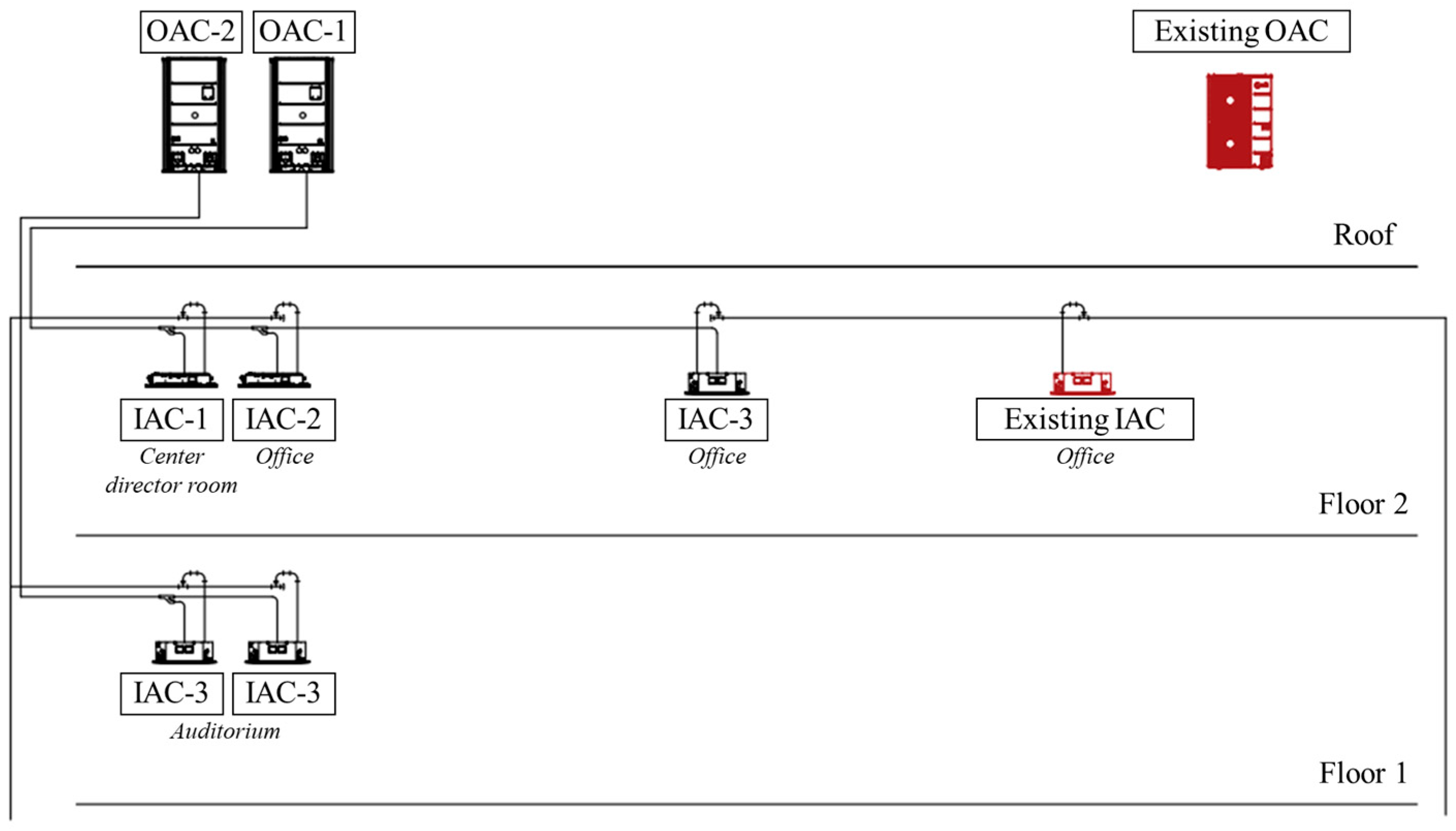
| OAC-1 | 23.3 kW | 25.9 kW | Case 1 | IAC-1 + IAC-2 | 7.2 kW | 8.1 kW | 31% | 50% |
| Case 2 | IAC-3 + IAC-3 | 26.0 kW | 28.6 kW | 112% | 110% | |||
| Case 3 | Case 1 + Case 2 | 33.2 kW | 36.7 kW | 142% | 130% | |||
| OAC-2 | 29.2 kW | 32.8 kW | Case 4 | IAC-3 + IAC-3 | 26.0 kW | 28.6 kW | 89% | 90% |
| Input | Output | ||
|---|---|---|---|
| Parameter | Set/From | Parameter | To |
| Return air temperature | Type56 | Supply air temperature | Type56 |
| Return air humidity | Type56 | Supply air humidity | Type56 |
| Return air flow rate | Type954c | Supply air flow rate | Type56 |
| Outdoor air temperature | Type9a | Cooling capacity | Type25c |
| Outdoor air humidity | Type9a | Heating capacity | Type25c |
| Control signal for cooling | Type108 | Power consumption | Type25c |
| Control signal for heating | Type108 | COP | Type25c |
| Outdoor unit ambient temp. | Type9a | ||
| Input | Output | ||
|---|---|---|---|
| Parameter | Set/From | Parameter | To |
| Heat source inlet temp. | 40 | Heating capacity | Type56 |
| Heat source flow rate | 36 LPM | Power consumption | Type25c |
| Heat sink inlet temp. | 20 | ||
| Heat sink flow rate | 36 LPM | ||
| Control signal | Type9a | ||
| Parameter | Name | Function |
|---|---|---|
| Type9a | Data reader | External data input |
| Type16a | Radiation processor | Tilted surface solar radiation |
| Type33e | Psychrometric chart | Psychrometric chart |
| Type69b | Sky temperature calculator | Sky temperature |
| Type56 | Multi-zone building | Building model |
| Type93 | Input value recall | Calculated data call |
| Type927 | Water-to-water heat pump | System boiler |
| Type954c | Air source heat pump | Electric heat pump |
| Type108 | 5 stage thermostat | Temperature control |
| Equation | Equa | Equation solver |
| Type65c | Online plotter | Simulation output |
| Type25c | Printer | Simulation output |
| Variable | Unit | R2 | RMSE | CVRMSE | ASHRAE Guideline 14 (Hourly) | Status |
|---|---|---|---|---|---|---|
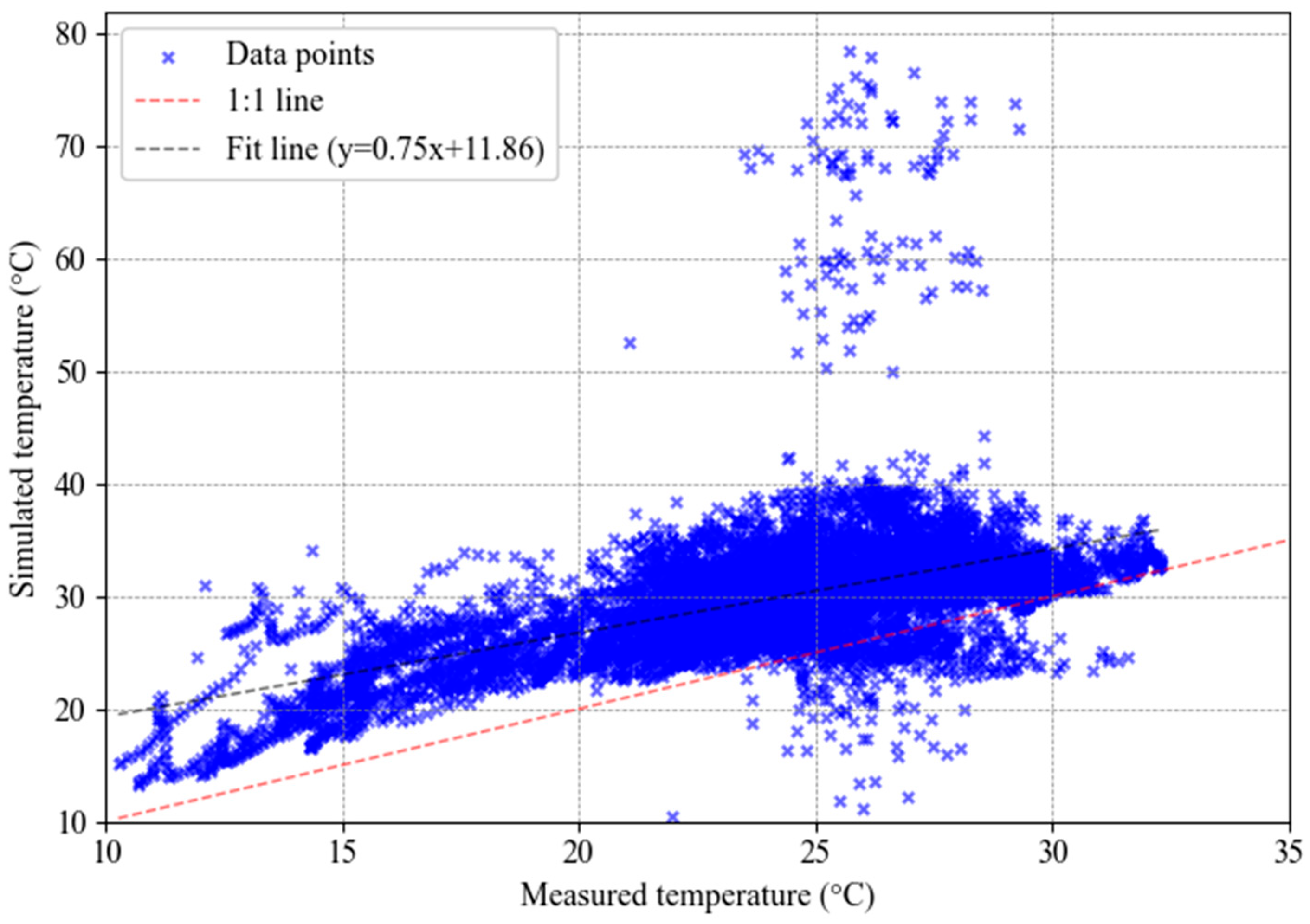
| Indoor Temperature | °C | 0.68 | 7.7–10.6 | 24.3–42.4% | N/A | Moderate Agreement |
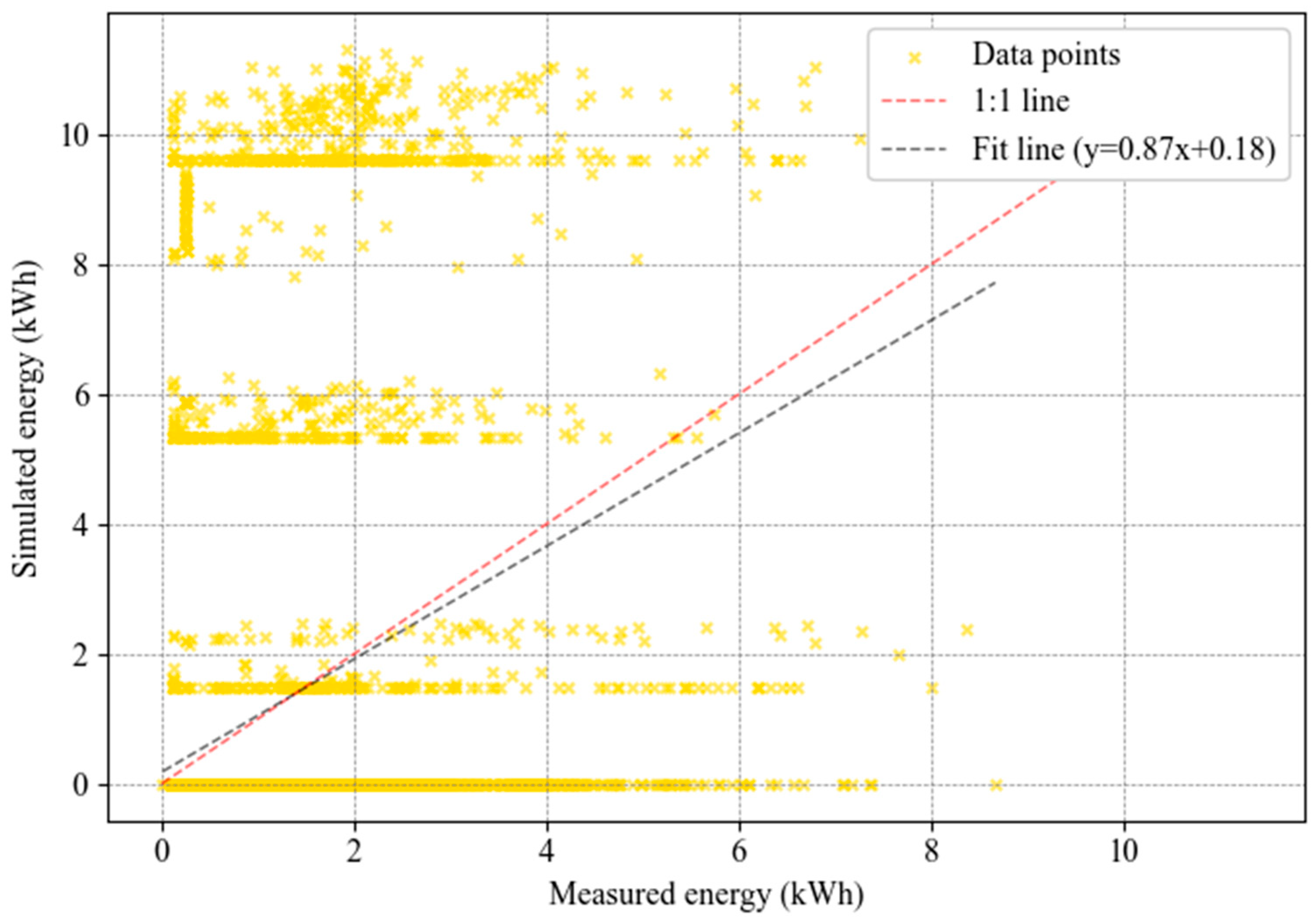
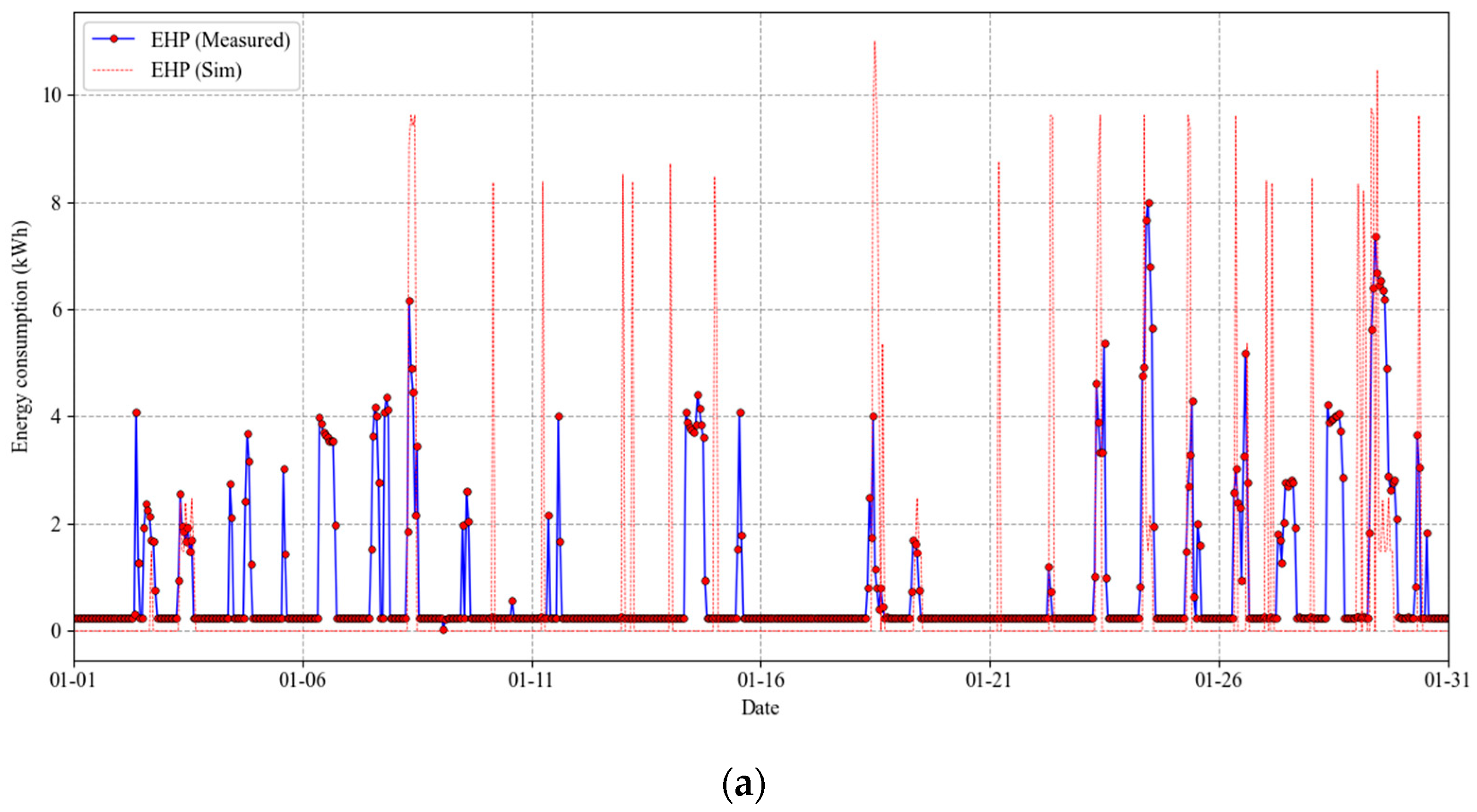
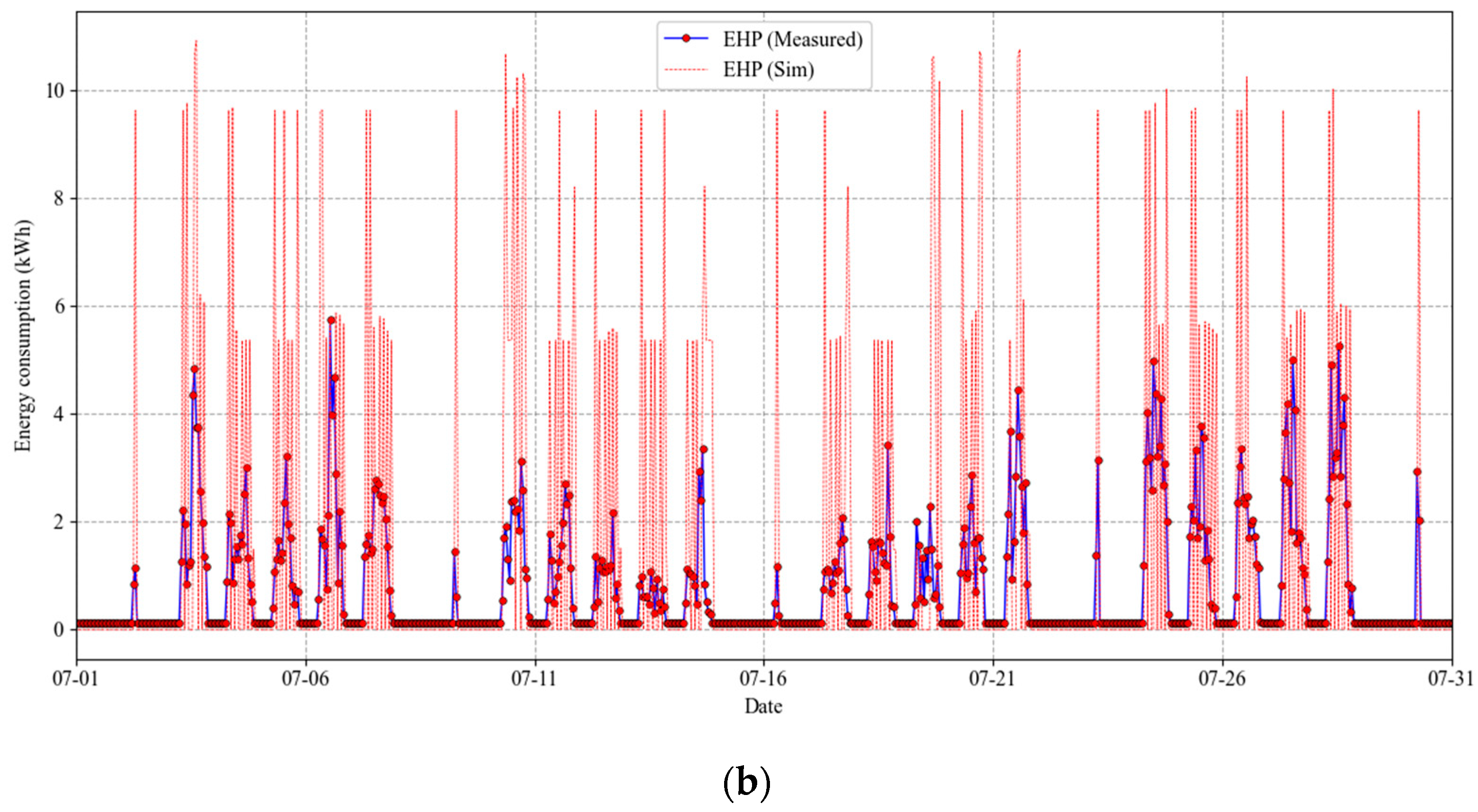
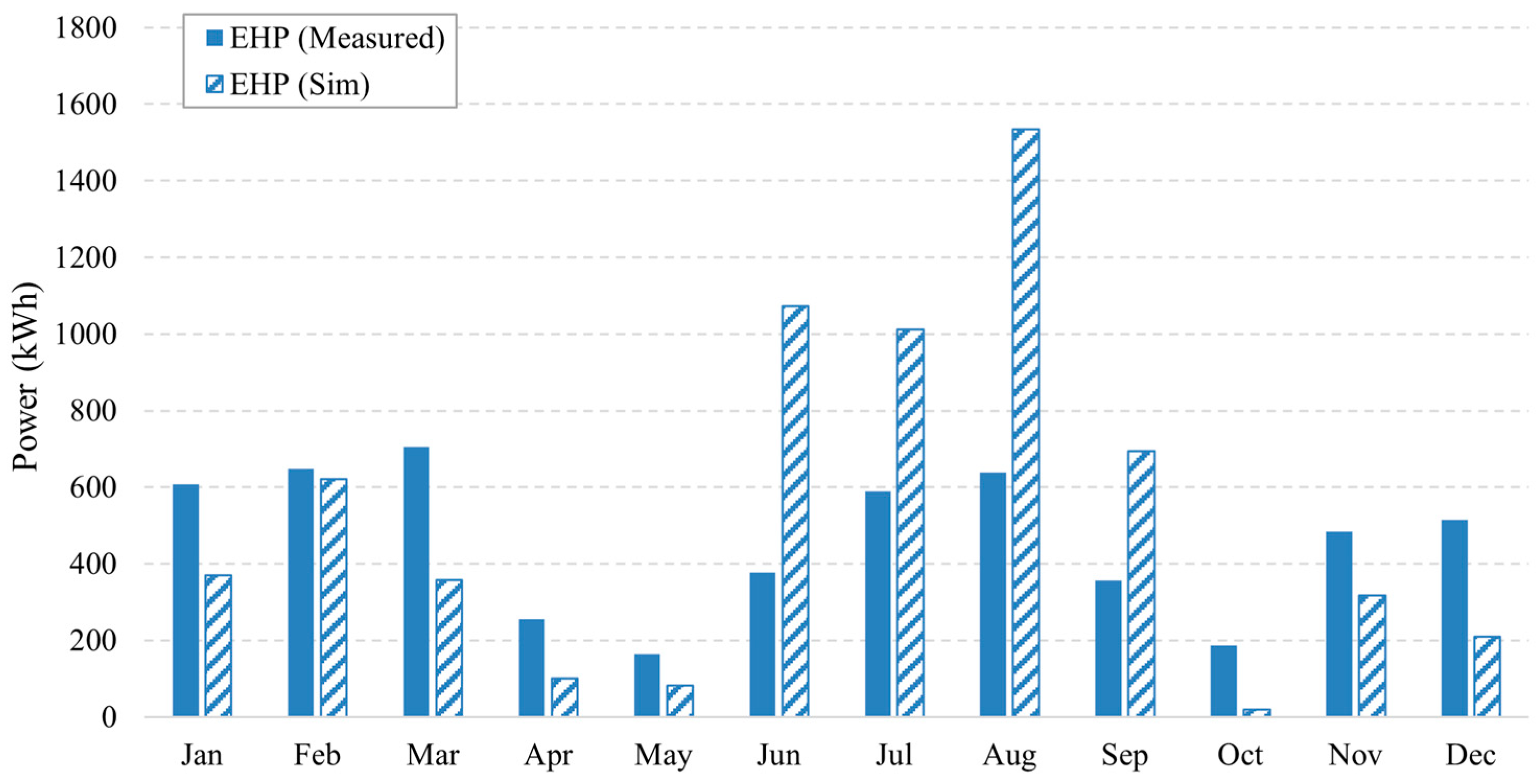
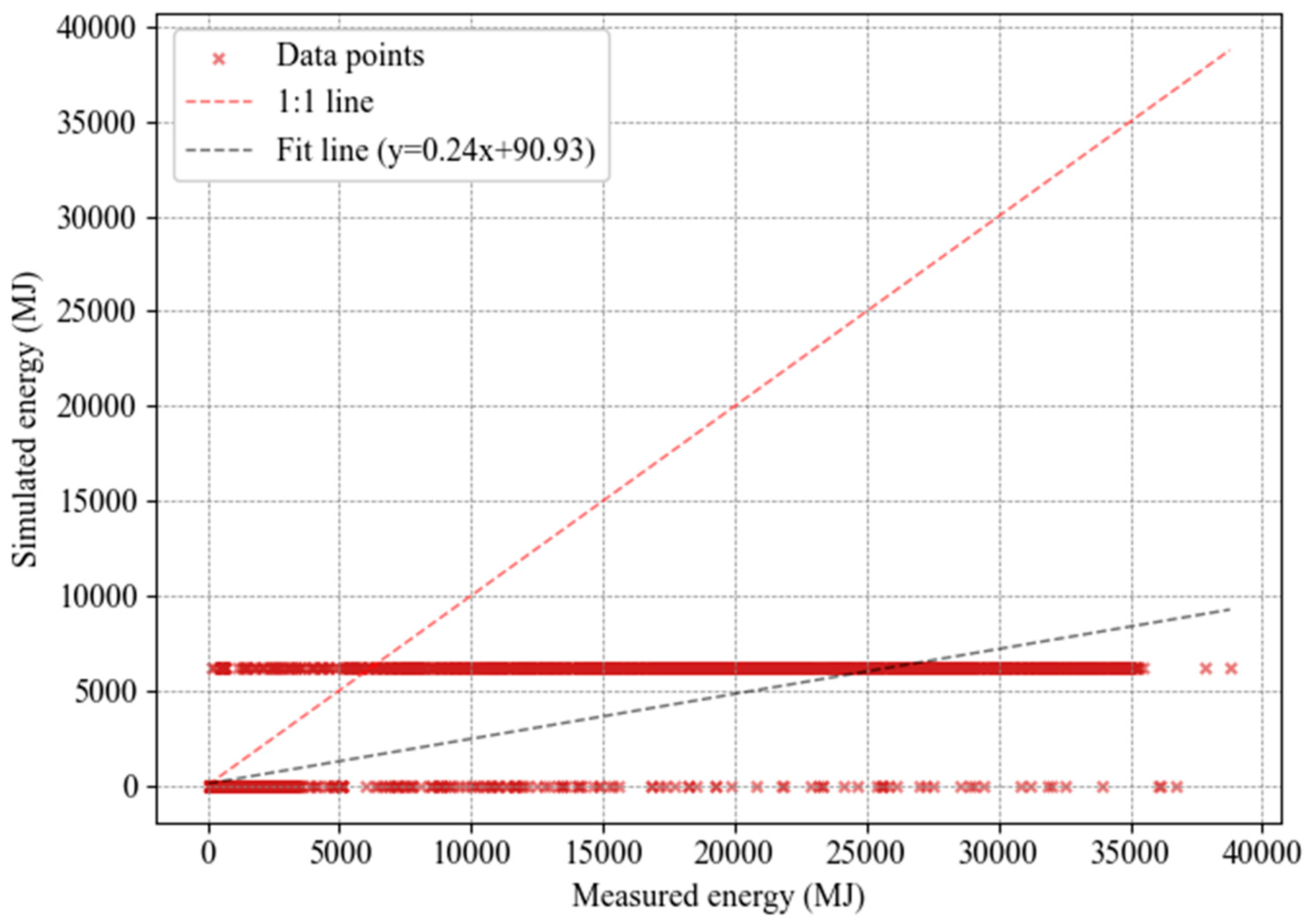
| VRF Electricity | kWh | 0.32 | 2.0–2.7 | 153–590% | <30% | Not Calibrated |
| Boiler Energy | MJ | - | 0.2–4.4 | 95–118% | <30% | Not Calibrated |
Disclaimer/Publisher’s Note: The statements, opinions and data contained in all publications are solely those of the individual author(s) and contributor(s) and not of MDPI and/or the editor(s). MDPI and/or the editor(s) disclaim responsibility for any injury to people or property resulting from any ideas, methods, instructions or products referred to in the content. |
© 2026 by the authors. Licensee MDPI, Basel, Switzerland. This article is an open access article distributed under the terms and conditions of the Creative Commons Attribution (CC BY) license.
Share and Cite
Kim, B.-J.; Yu, K.-H.; Yoon, S.-H.; Lim, H. Proxy-Calibration Approach for Transient Simulation of Variable Refrigerant Flow Systems in Energy Performance Assessment of an Existing Building. Buildings 2026, 16, 210. https://doi.org/10.3390/buildings16010210
Kim B-J, Yu K-H, Yoon S-H, Lim H. Proxy-Calibration Approach for Transient Simulation of Variable Refrigerant Flow Systems in Energy Performance Assessment of an Existing Building. Buildings. 2026; 16(1):210. https://doi.org/10.3390/buildings16010210
Chicago/Turabian StyleKim, Beom-Jun, Ki-Hyung Yu, Seong-Hoon Yoon, and Hansol Lim. 2026. "Proxy-Calibration Approach for Transient Simulation of Variable Refrigerant Flow Systems in Energy Performance Assessment of an Existing Building" Buildings 16, no. 1: 210. https://doi.org/10.3390/buildings16010210
APA StyleKim, B.-J., Yu, K.-H., Yoon, S.-H., & Lim, H. (2026). Proxy-Calibration Approach for Transient Simulation of Variable Refrigerant Flow Systems in Energy Performance Assessment of an Existing Building. Buildings, 16(1), 210. https://doi.org/10.3390/buildings16010210