


Abstract
This study presents an integrated ex-post evaluation of a municipal window-retrofit program in Goyang, Republic of Korea (heating-dominated, Dwa). Using field surveys and pre- and post-utility bills for 36 dwellings, mainly pre-2000 low-rise reinforced-concrete buildings, we normalize climate with HDD and CDD and prices with CPI-deflated tariffs to isolate the intrinsic effect of window replacement. Area-normalized indicators (, , DPB, NPV, AC) were computed. Average annual savings were 30.2 kWh per m2 per year ( ≈ 16 percent), consisting of 10.6 kWh per m2 per year of gas and 19.6 kWh per m2 per year of electricity (n = 36). The median discounted payback was 7.0 years. Under a 50 percent subsidy, about 80 percent of projects recovered private investment within 15 years and showed positive NPV with a median of about USD 4944. The electricity-tariff multiplier had the largest influence on cash flows and payback. The median abatement cost was about USD 352 per tCO2-eq. A portfolio view indicates that prioritizing low-cost cases maximizes total abatement, and that higher-cost cases merit design or cost review. Using the first post-retrofit year 2023, portfolio abatement is about 623 tCO2-eq per year. The framework jointly normalizes climate and price effects and yields policy-relevant estimates for heating-dominated contexts.
1. Introduction
The building sector accounts for approximately 36% of global energy consumption [1] and 34% of global carbon emissions [2], and it is widely recognized as pivotal for meeting national mitigation targets. Regulatory measures for new construction and high-efficiency design alone are often insufficient for achieving near-term carbon reduction [3]. Consequently, performance upgrades to existing building stock through retrofit interventions are increasingly regarded as a promising solution [4,5,6]. Governments and cities worldwide are advancing building-efficiency policies and supporting retrofit projects to accelerate progress toward carbon neutrality. In the European Union, recent revisions to the Energy Performance of Buildings Directive (EPBD) introduced mandatory phased renovations of poorly performing buildings [1,7]. North America [6,8,9,10] has expanded tax credits and rebate programs to mobilize private-sector participation. In major Asian cities, including those in South Korea, retrofit initiatives are being implemented to reflect local climatic and economic conditions [11]. Collectively, these developments indicate a global trend in which public policies and private markets mutually reinforce the demand for building retrofits [7].
However, unlike new construction, retrofit outcomes are shaped by heterogeneous pre-existing conditions, including physical configurations, local climate, and occupant behavior [5,8,10,12]. As a result, gaps between predicted and realized performance readily emerge, and both technical outcomes and economic viability vary substantially across urban contexts, climatic zones, and building typologies. This variability is a major source of uncertainty that hinders broader adoption of retrofit projects [3,5,9]. Although some dispersion is unavoidable, the absence of credible, validating evidence to substantiate expected outcomes can undermine the continuity of public programs and discourage private investment [3,13]. Because prediction–performance gaps persist, pre-retrofit simulations remain useful for screening options but should be complemented by ex-post analyses based on measured savings [3,14]. Moreover, identical energy savings can correspond to widely different costs per kWh, payback periods, and marginal abatement costs depending on the initial investment and cost structure. Accordingly, building on ex-post evidence, an integrated evaluation of both energy outcomes and construction costs is required. Such evaluations clarify the benefits per unit investment and enable concurrent assessments of policy effectiveness, economic payback, and prospects for sustained private-sector engagement [3,7,15].
Simulation-based studies explore retrofit strategies and compare design alternatives prior to implementation, using methods such as single-measure envelope analyses, archetype or surrogate stock models, and BIM-based life-cycle frameworks that integrate design, construction, and operations [14,16,17,18,19,20,21,22]. While these approaches support ex-ante decision-making, they are constrained when tested against operational data. Empirical analyses consistently show that simulation-based or engineering-model projections often overestimate real-world savings [8]. Large-scale program evaluations, for example, report realized savings that are 30–50% lower than engineering-model predictions [6], while occupant behavior and control settings can still account for up to a two-fold variation in heating demand [12]. In short, simulation and optimization remain essential for exploring retrofit scenarios, but bridging the simulation–reality gap through empirical, post-retrofit evidence is critical for substantiating real-world effectiveness.
Empirical ex-post studies have documented the specific retrofit measures implemented and the actual magnitude of savings achieved [7,9,10,11,23,24,25,26,27]. Across public, social, and mixed residential buildings, interventions such as insulation reinforcement, window replacement, and heating-control optimization have yielded 15–35% annual energy reductions [7,9,10]. Although realized savings are often 10–25% lower than predictions, this variation empirically illustrates how differences in building characteristics and control environments shape actual performance outcomes [28]. Several studies have examined the effectiveness of individual technical interventions [24,25,26]. For example, Eriksson and Lidelöw [25] reported 25–30% reductions in heat loss following window replacement in Swedish multi-family dwellings, whereas [24] observed 18–22% reductions in heating load through envelope reinforcement and double glazing in Korean apartment buildings, also identifying diminishing marginal benefits beyond certain insulation thresholds. Despite variability across studies, these empirical evaluations are valuable because they identify specific measures and the corresponding magnitudes of savings under diverse conditions, collectively demonstrating that retrofits deliver measurable, context-sensitive improvements in building performance.
However, recognizing that a retrofit delivers savings does not automatically answer the next practical question: which retrofit works best? Because no single measure is universally optimal, a more contextual question arises: which option works best for this building, with this budget, in this context? These issues remain unresolved for both policymakers and practitioners. Indeed, large-scale U.S. programs have shown that although energy savings are consistently achieved, net economic losses can emerge once total expenditures are considered [9]. Consequently, in older or low-income housing, high upfront costs, long payback periods, and uncertainty remain critical barriers to adoption [3]. Moreover, cost not only determines whether retrofits occur but also directly influences how outcomes and policy effectiveness are interpreted. In Switzerland, subsidy analyses revealed that identical energy reductions can yield widely different cost efficiencies depending on program design and free-rider rates [7]. Thus, the key issue is not merely how much energy is saved, but how much each unit of saved energy costs and whether such investments are financially viable. Cost-effectiveness is not a secondary consideration; it frequently determines whether retrofits take place at all. Within these constraints, energy efficiency must be understood not as a purely technical endeavor but as an outcome shaped by investment, finance, and market structure [13]. Ultimately, if empirical research has demonstrated which measures save energy and by how much, the next essential step is to determine whether these savings are truly worth their cost. This represents a necessary shift from energy performance to economic value, and from technical validation to policy and market realism.
In examining these economic dimensions, previous research on building energy retrofit economics has largely relied on predictive, ex-ante approaches such as Life Cycle Cost Analysis (LCCA), Life Cycle Assessment (LCA), and social cost–benefit analysis (CBA) [15,27,29,30,31,32]. However, these studies depend heavily on assumed parameters and input conditions, and only a limited number have verified post-retrofit operational outcomes using measured data. This limitation arises primarily because collecting reliable post-retrofit datasets is difficult, cost information from individual projects is rarely disclosed, and matching energy-use data with actual construction costs presents significant methodological challenges [27,30]. Integrated frameworks that normalize measured savings and link them to cost and carbon outcomes remain scarce. Social CBA studies have mainly examined public investment appraisals, capturing social welfare (net social benefit) and non-market values such as carbon reduction, health improvements, and housing quality [15,27,29]. In contrast, household-level private economic considerations, such as individual payback, abatement cost, and perceived efficiency, have rarely been analyzed or have been addressed only partially. This gap reflects the confidentiality of micro-level cost data and the misalignment between administrative and household records [15,29]. As a result, analytical frameworks that integrate both social and private perspectives remain underdeveloped. Most previous studies also investigated deep retrofit projects involving multiple combined measures, such as insulation, window replacement, and HVAC upgrades, rather than analyzing single measures separately [27,31]. This trend reflects the practical reality that retrofit projects are typically implemented as composite packages, making it difficult to isolate the cost and performance of individual interventions. The absence of standardized accounting structures to disaggregate cross-measure cost interactions further limits these analyses [31]. Consequently, evidence on the standalone cost-effectiveness of single measures remains limited. In addition, most studies reported results as national or regional averages, while only a few explored the variability or distribution of cost-effectiveness across households [27,29,30]. This is largely due to small sample sizes and heterogeneous data quality, which hinder statistically robust distributional or heterogeneity-focused analyses. As a result, existing research has struggled to explain the uneven performance of retrofit outcomes and the differential impacts of policy interventions. Finally, there is a noticeable shortage of empirical research quantifying the impact of policy instruments, such as subsidies or tax incentives, on actual energy savings and investment payback [15,27,29]. Although some studies have discussed the social benefits of support schemes, regional diversity in subsidy design and the complexity of policy variables have made quantitative integration into cost models challenging [15,27]. Few studies have therefore empirically assessed how public incentives influence private investment behavior or the marginal efficiency of carbon abatement. In summary, five critical gaps exist in the literature:
- (1)
- limited ex-post, measurement-based energy–cost–carbon integration;
- (2)
- insufficient inclusion of both social and private perspectives;
- (3)
- lack of single-measure cost-effectiveness evaluation;
- (4)
- minimal attention to distributional or heterogeneity analysis; and
- (5)
- scarce quantitative evaluation of subsidy effects.
To address these limitations, this study conducts an empirical analysis of residential retrofit projects currently being implemented in the Republic of Korea. In recent years, both the national government and local municipalities have launched a variety of housing energy-efficiency initiatives, with public programs increasingly supporting upgrades to windows, thermal insulation, and building services in aging dwellings. This policy diffusion provides expanded opportunities to rigorously quantify the realized costs and energy-saving effects of actual retrofit interventions—precisely the type of ex-post evidence that remains scarce in previous research. Against this backdrop, we focused on Goyang City in the northern Seoul metropolitan area (≈37.6° N), a temperate city at a mid-latitude comparable to that of heating-intensive cities such as Beijing and Columbus, Ohio. Goyang has a long-term annual mean outdoor temperature of approximately 11.9 °C [33], and nearby Seoul records annual heating degree days (HDD; base 18 °C) on the order of 2400–2600 °C·day in recent years [34]. These statistics indicate a heating-dominated climate with relatively low mean temperatures. In 2022, under the city’s Housing Energy Efficiency Program, multiple retrofit projects targeting older homes were implemented, with a primary emphasis on window replacement. Executed within a common timeframe and under comparable conditions, these subsidized retrofit projects are well suited for empirically examining the linkage between costs and energy savings while minimizing exposure to external confounding factors.
Using this empirical dataset, this study conducts an integrated analysis of retrofit performance by objectively normalizing energy savings and costs. This approach quantitatively identifies the interrelationships among energy savings, carbon reduction, and cost-effectiveness, thereby directly addressing the previously noted lack of ex-post, measurement-based integration and the limited empirical validation of single-measure retrofits. The resulting framework establishes an analytical foundation for reducing uncertainty surrounding retrofit outcomes and enhancing the credibility of subsequent policy evaluations, program designs, and private investment decisions. Moreover, the integrated assessment framework proposed here provides practical implications for residential retrofit policymaking not only in Korea but also in other cities characterized by monsoon-influenced continental climates with low mean temperatures and pronounced heating demand.
2. Data & Methods
2.1. Overview of the Retrofit Program
The municipal retrofit program in Goyang, Republic of Korea, supported approximately 300 houses between 2021 and 2024, with an emphasis on low-rise dwellings. Most participating homes were detached houses or three-story multi-family buildings, and 91.43% were built in 2000 or earlier. High-rise apartment complexes were not included. Located in the northern Seoul metropolitan area at approximately 37.66° N, Goyang experiences cold, dry winters and hot, humid summers and is classified as Dwa in the updated Köppen–Geiger climate system [35]. Recent summers have trended hotter, making both winter heating and summer cooling increasingly energy-significant. The city’s latitude is slightly south of Columbus, Ohio (~39.96° N; humid continental Dfa) and close to Beijing (~39.9° N; Dwa), both of which represent continental climates with pronounced seasonal extremes. According to Korea Meteorological Administration (KMA) climate normals (1991–2020), Goyang’s long-term annual mean outdoor temperature is approximately 11.9 °C [33]. The winter heating design outdoor dry-bulb temperature for nearby Seoul is −11.3 °C, as specified in Korea’s Standards for Energy-Saving Design of Buildings (Annex Table 7) [36], which list heating design conditions for 17 reference cities. Neighboring areas, including Goyang, are instructed to apply the nearest reference values.
Figure 1 presents representative samples of the program’s target housing types—detached houses (a–c) and multi-family buildings (d–f). Each case includes an exterior view, a simplified floor plan, and close-ups of the retrofit target windows. The close-ups (c, f) reveal single glazing, prominent thermal bridging at aluminum frames, degraded seals (poor airtightness), and visible condensation traces, all consistent with high window U-values and air leakage under increasingly stressed continental climates. The prioritization of fenestration upgrades also reflects typical construction conditions. In reinforced concrete structures with wet-wall construction, installing additional wall insulation is complex, disruptive, and costly. In multi-family buildings, roof insulation is difficult to implement at the unit level because the roof is a shared structural element. Under these constraints, window replacement—readily implementable at the dwelling level with occupants in place—naturally became both the most requested option and the de facto municipal preference, aligning with its role as a practical passive measure. From a thermal comfort perspective, window upgrades increase interior surface temperatures and reduce façade downdrafts. At a given thermostat setpoint, this mitigates local cold discomfort and reduces the reliance on plug-in electrical spot heating during winter (e.g., portable heaters or electric/hot-water heating pads or blankets).
Figure 1.
Examples of detached and multi-family houses for window retrofits. (a–c) Detached house: exterior view, simplified floor plan indicating window locations, and close-up photos showing deteriorated aluminum frames and condensation traces. (d–f) Multi-family house: exterior view, floor plan, and close-up views of aged single-glazed windows with poor sealing.
The program’s primary intervention was full window replacement, targeting reduced window U-values (thermal transmittance) and lower air leakage to improve passive envelope performance. High-performance assemblies combined Low-E double or triple glazing, argon (Ar) gas fill, warm-edge spacers, and insulated frames. All installed products met the Korean window energy-efficiency labeling scheme (Grades 1–3). Post-retrofit U-values and SHGC varied across dwellings but remained within a relatively narrow high-performance range. Specifications emphasized quantitative U-value reduction: most installations used double glazing (overall thickness ≈ 22–24 mm), while some homes upgraded to triple glazing (≈40–52 mm) to achieve lower U-values (e.g., double glazing: Low-E 5–6 mm/Ar 12 mm/clear 5–6 mm; triple glazing: Low-E 5 mm/Ar 16–18 mm/clear 5 mm/Ar 16–18 mm/Low-E 5 mm). The municipal support scheme did not modify exterior shading devices and did not perform project-specific optimization of SHGC beyond certified product ranges. As a result, SHGC and shading conditions were not treated as explicit design variables in the analysis but instead considered part of dwelling-level heterogeneity. Accordingly, our ex-post evaluation infers realized performance from pre- and post-retrofit utility bills under these program-standard window upgrades, rather than assuming a uniform U-value or SHGC across all cases.
This study analyzed a subset of program-funded projects for which pre- and post-retrofit documentation and utility records were complete and comparable; files with incomplete or inconsistent records were excluded to maintain analytical integrity. Applications were ranked by a city-convened expert review panel using a concise scoring sheet across three axes: dwelling size, observed deterioration, and project cost, with bonus/malus adjustments. Each file included a photo-and-plan dossier documenting pre-retrofit conditions (e.g., window counts and locations, visible aging such as condensation traces and degraded seals) and an itemized cost review with inclusion/exclusion flags, which was examined for baseline thermal performance information. Files lacking verifiable efficiency data were excluded. In practice, this review process functions more as a light screening than a detailed engineering assessment. It does not incorporate physics-based building simulations or calibrated pre-retrofit energy modeling; rankings rely primarily on photographic evidence of deterioration and cost reasonableness, with pre-retrofit energy-use histories serving only as supplementary documentation. Nonetheless, this approach is pragmatic and defensible under constraints of scale, budget, and time, enabling the rapid triage of aging homes. Ideally, a stepwise procedure (pre-retrofit prioritization based on anticipated savings followed by post-retrofit verification of realized performance and cost-effectiveness) would be desirable. For approved cases, costs were shared under a matching-fund scheme in which the municipality co-funded a portion of the retrofit, while the applicant paid the remainder. The current program does not include systematic post-retrofit monitoring or analysis. To accurately quantify impacts, additional post-retrofit data collection and evaluation were required, which were undertaken in this study.
2.2. Field Survey and Data Collection
From July to August 2024, two field researchers conducted in-person surveys and brief interviews (approximately 30–60 min). Of the 127 projects completed by 2022, 74 dwellings agreed to site visits and completed the field survey (visit response = 74/127 = 58.3%). After scheduling and post-survey data checks, cases with incomplete application records or inconsistencies between the application and field survey were removed, resulting in 36 dwellings with fully linkable data (final usable = 36/74 = 48.6%; overall = 36/127 = 28.3%). The study fell outside formal Institutional Review Board (IRB) requirements. All participants provided informed consent; addresses were anonymized (with coarsened geolocation when applicable), and non-essential personal identifiers were masked and destroyed after data linkage. The survey teams also photographed interiors and exteriors to document physical conditions.
Utility records were obtained from billing statements submitted by participants. Electricity usage was recorded directly in kWh, and gas usage was also reported in kWh on the bills; thus, no additional higher heating value (HHV) conversion was required. For the pre-retrofit baseline (2020–2021), one representative value per calendar month was constructed from the two annual records while accounting for vacancies. When both years showed positive (non-zero) usage for a given month, the arithmetic mean was used. When one year showed zero usage due to vacancy and the other showed positive usage, the non-zero value was adopted. When both years showed zero usage, the baseline value was set to zero for that month. This vacancy-adjusted averaging provides annual representativeness even for partially vacant units.
Table 1 summarizes the physical and energy-use characteristics of the 36 surveyed dwellings. The energy-use variables reflect annualized, area-normalized raw energy use. Pre-retrofit values were calculated as the vacancy-adjusted mean of the 2020–2021 records, and post-retrofit values correspond to the 2023 single-year totals (the first full operating year after retrofit). Using this approach, mean pre-retrofit gas and electricity intensities were 140.4 and 34.5 kWh/(m2·yr), respectively, decreasing to 119.9 and 33.2 kWh/(m2·yr) after retrofit. The sample consists mainly of small- to medium-sized dwellings (mean 105.65 m2), constructed between 1985 and 2004 and typically occupied by 2–3 residents; approximately 91.7% are small multi-family buildings (≤3 stories), with the remainder being detached houses. The number of occupants denotes the household size of each participating dwelling. Follow-up interviews indicated that all households used at least two types of plug-in electric heating devices, with nearly universal electric or hot water mats. Hours of operation and output levels were not recorded; this behavioral information is used solely for contextual interpretation.
Table 1.
Descriptive statistics of follow-up household survey.
Regarding the opaque envelope, the surveyed dwellings exhibit similar low-rise construction characteristics. Built between 1985 and 2004, the 36 houses in Goyang City (central climatic region) generally feature reinforced concrete or concrete block exterior walls finished with brick or siding, and either flat reinforced-concrete slabs or lightweight pitched roofs. Municipal application records and field visits confirmed that no major wall or roof retrofits occurred during the program period. Detailed as-built drawings and layer-by-layer construction records were not available; therefore, exact envelope configurations could not be reported. Instead, we briefly summarize the national energy-saving design criteria that formed the regulatory background during the period of construction. For the central region that includes Goyang, these provisions specified, for example, a maximum wall U-value of 0.5 kcal/(m2·h·°C) (≈0.58 W/m2K) and insulation thicknesses of approximately 50 mm for exterior walls and 80 mm for roofs in the mid-1980s. These requirements were strengthened in later revisions, including the 2001 Energy-Saving Design Criteria, which increased insulation thicknesses for both walls and roofs. These code values are cited only as reference points for envelope performance requirements at the time; they do not imply strict compliance or uniform construction across all dwellings. Given this documented context and the absence of major envelope retrofits, the performance changes discussed in Section 3.1, Section 3.2, Section 3.3 and Section 3.4 are interpreted primarily as the effects of window replacement on an otherwise unchanged opaque envelope, with the understanding that operational and behavioral factors may also influence observed outcomes.
Figure 2 shows that floor areas cluster within the 60–120 m2 range, with a small right tail above 180 m2 corresponding to larger detached houses. Because only cases with complete application and field survey records were included, better-documented dwellings may be somewhat overrepresented, and the final sample size (n = 36) remains modest. Accordingly, this study is framed as a descriptive portfolio assessment of the usable program cohort rather than as a statistically representative sample of all low-rise dwellings in Goyang. To quantify pre- and post-retrofit effects accurately, the energy-use variables are adjusted (normalized) in Section 2.4.
Figure 2.
Distribution of floor area among the surveyed dwellings.
2.3. Variable Definition and Area Normalization
To enable consistent comparison across heterogeneous dwellings, all variables were explicitly defined and standardized on an area-normalized basis. In this study, electricity use refers to the sum of cooling and base loads, together with winter plug-in spot heating, whereas gas use primarily represents space heating and domestic hot water. This categorization affects only cost weighting and does not influence the HDD/CDD-based climate classification described in Section 2.4.1. Each dwelling i was represented by its gross floor area (m2), which served as the denominator for all energy-use indicators. Monthly electricity and gas consumption before and after retrofitting (, ) were obtained directly from the billing records described in Section 2.2 and converted to area-normalized values (). This step removes size-related bias between detached and multi-family dwellings and enables direct comparison based on energy intensity.
Derived variables were subsequently computed to quantify climate-adjusted monthly and annual energy use, costs, and carbon outcomes. These include climate-adjusted unit consumption (), annual savings per unit area (), total annual savings (), real and nominal retrofit costs (, ), unit costs (, ), and derived indicators such as real annual savings (), discounted payback (), and abatement cost ().
All monetary quantities were converted to real 2024 USD to ensure temporal consistency for the economic analysis-. Project expenditures originally denominated in KRW were converted using a fixed rate of 1 USD = 1200 KRW. This mid-range value reflects recently higher KRW/USD exchange levels and approximates the 2015–2024 multi-year average. It was selected to minimize timing noise and improve reproducibility using official exchange rate data from the OECD Main Economic Indicators, the World Bank “official exchange rate (LCU per US$, period average)” database, and the Bank of Korea Economic Statistics System (ECOS) [37,38,39].
Table 2 summarizes the full variable system and symbol–dataset mapping used in the study. It provides a transparent link between the original survey and billing records and the normalized analytical variables used in subsequent computations, forming a consistent foundation for later climate and price adjustments (Section 2.4).
Table 2.
Variable definitions and symbol–dataset mapping.
2.4. Climate and Price Normalization
This section addresses the removal of external distortions arising from climatic and economic differences between the pre- and post-retrofit periods. Climate normalization adjusts energy use to a common reference climate, ensuring that variations in heating and cooling demand reflect only building efficiency rather than weather fluctuations. Price normalization converts energy tariffs and costs to real-price values that account for inflation and tariff escalation, enabling accurate estimation of retrofit-related expenditures and monetary savings. Together, these procedures ensure that the evaluated energy and economic outcomes reflect the intrinsic effects of the retrofit measures rather than external temporal factors.
2.4.1. Climate Normalization
To account for climatic variations, energy use was normalized using heating and cooling degree days (HDD and CDD). The monthly normalized energy consumption for building , fuel type , and month was calculated using Equation (1):
where and represent the monthly degree days for the reference climate. The reference year was defined as the mean of 2020–2021, representing the two-year pre-retrofit period.
HDD and CDD were calculated from daily mean outdoor temperature records for Goyang (2020–2023) [40] using national base temperatures for Korea ( ). For each month of year , with average temperature and number of days , HDD and CDD were computed as follows:
Annual HDD and CDD values were obtained by summing monthly values. Figure 3 illustrates the monthly distributions of HDD and CDD for Goyang from 2020 to 2023. Consistent seasonal patterns are evident, with heating loads (HDD) dominating colder months and cooling loads (CDD) increasing sharply during summer.
Figure 3.
Monthly HDD and CDD for Goyang (2020–2023).
Table 3 shows the annual totals and corresponding normalization factors. The post-retrofit year (2023) experienced a 4.1% reduction in HDD relative to the pre-retrofit reference (2020–2021 average), whereas CDD increased by approximately 47.6%, indicating a substantially warmer summer. These results underscore the necessity of climate normalization prior to evaluating retrofit-induced energy savings. In this paper, “heating-dominated” refers strictly to HDD/CDD–based climate characterization and is independent of the relative shares of gas versus electricity savings.
Table 3.
Annual HDD/CDD and climate normalization factors ( = 18 °C/ 26 °C).
2.4.2. Price Normalization
Following climatic normalization, price normalization was applied to express all energy tariffs and monetary values in real terms, thereby eliminating inflationary and temporal distortions between the pre- and post-retrofit periods. This ensured that cost-related indicators reflected only the intrinsic economic performance of the retrofit measures rather than external price fluctuations. In this study, “real” refers to CPI-deflated values expressed in the 2024 base year; all nominal tariffs and costs were converted prior to economic evaluation to remove the effect of inflation.
Because consumer price index (CPI) data were available as year-over-year growth rates , the CPI ratio between the base year and the nominal tariff reference year reconstructed by chaining the annual growth factors, as shown in Equation (3):
The CPI data were obtained from Statistics Korea’s KOSIS portal (National Indicators, Index Nuri) under “Consumer Price Index for Housing, Water, Electricity, and Fuels” [41]. The base and reference years were set to and . The nominal tariffs for each fuel type were converted to real base-year tariffs as shown in Equation (4):
Because and , the chained CPI ratio in Equation (3) reduces to a single annual factor (). The product form is retained for generality, allowing direct extension to cases in which the base and reference years differ by more than one year.
All energy-related costs are expressed in real 2024 USD. The following unit conversions were applied consistently for tariff harmonization:
For natural gas, retail tariffs were based on publicly disclosed regional city gas rates compiled by the Korea City Gas Association, a nonprofit organization that aggregates and publishes supplier tariffs [42]. These tariffs operate under the national wholesale supply framework of the Korea Gas Corporation (KOGAS) [43]. Because all retrofit projects were located within the same supply area, a single regional tariff schedule was applied, corresponding to an average unit price of USD 0.0676 per kWh (real@2024), derived from the CPI-adjusted residential usage component. Only proportional usage-based components were included; fixed or non-variable charges such as basic fees and VAT were excluded. Electricity tariffs followed the residential low-voltage structure of the Korea Electric Power Corporation (KEPCO; sourced from https://www.kepco.co.kr (accessed on 30 October 2025)), including tiered and seasonal (summer/other) schedules. Only per-kWh components directly affected by usage were considered—specifically, the energy charge, climate–environment charge, and fuel adjustment charge—resulting in real 2024 rates of USD 0.105/0.183/0.261 per kWh, with the super-user tier (>1000 kWh/month) set at USD 0.607 per kWh.
To avoid ambiguity, all growth-rate calculations in this section use CPI-deflated (2024-base) tariff series. “Real annual growth” denotes the compounded average annual increase over each window. All escalation rates are reported as %/yr (real).
After conversion to real terms, fuel-specific real escalation rates () were derived to capture long-term structural trends in tariff growth beyond inflation, enabling consistent projection of real energy costs in the subsequent financial analysis. For each fuel, was computed from recent CPI-deflated tariff histories as the midpoint between two observation windows that reflect different aspects of underlying price dynamics. For electricity, the windows 2019–2024 (medium-term adjustments) and 2021–2023 (recent high-volatility period) were used, and the midpoint of the corresponding real annual growth rates was adopted as the baseline escalation rate. For city gas, major tariff changes occurred in the very recent period around 2023–2024 and were implemented through regional suppliers; thus, shorter windows centered on 2023 were used. Accordingly, was obtained as the midpoint between the real growth rates for 2023–2024 and 2023–2025. This midpoint approach avoids overstating economic performance by relying solely on the steepest recent increases, while also avoiding excessive conservatism that would understate the likelihood of continued tariff growth under evolving energy and climate-policy conditions. The resulting CPI-deflated (2024-base) baseline tariffs and fuel-specific escalation rates are summarized in Table 4 and are used in the economic evaluation (Section 2.6).
Table 4.
Real escalation rates of natural gas and electricity tariffs.
2.5. Energy Savings Computation
After applying climatic and price normalization (Section 2.4), energy savings were computed on an area-normalized basis to ensure comparability across dwellings. For each building and fuel type (electricity, gas), the annual normalized energy savings per unit area () were calculated using Equation (5):
where and denote monthly, climate-adjusted consumption before and after retrofitting, respectively. The annual energy-saving ratio () was derived from total annual energy use before and after retrofit (Equation (6)):
No end-use disaggregation was performed. Electricity savings were evaluated at the fuel-bill level without allocating shares to cooling or plug-in spot heating. For descriptive purposes, combined indicators across both fuels were defined on a final-energy basis by summing gas and electricity savings per unit area in kWh/(m2·yr), as in Equation (7). This “total” indicator is not a primary-energy metric; it is used only to summarize end-use savings across fuels.
Figure 4 summarizes the empirical distributions of the energy-saving indicators. Figure 4a,b present the raw histograms of and , for electricity, gas, and their total. Most values are positive, indicating overall post-retrofit reductions, although a few negative cases remain. Gas consumption exhibits a wider dispersion than electricity, whereas electricity shows a narrower and more concentrated distribution. The combined distribution (Figure 4a) shifts further to the right because it reflects the additive contributions of both fuels to total unit-area savings, while the combined distribution (Figure 4b) lies between the two fuel-specific distributions, as it represents a relative ratio rather than an absolute sum. Figure 4c,d show the kernel density curves for and , after interquartile-range (IQR) filtering, where outliers are removed using the criterion . After filtering, variance decreases and the alignment between mean and median improves, while central tendencies remain consistent (). These results confirm that the climate-normalized dataset yields stable and interpretable savings indicators, validating the computational procedure and providing a reliable foundation for the analyses presented in Section 3 (Results).
Figure 4.
Distributions of normalized energy-saving metrics ( and ) before and after IQR filtering.
2.6. Economic Assessment Based on Normalized Energy and Price Data
2.6.1. Evaluation Framework and Assumptions
This section evaluates the economic performance of the retrofit measures using the climate- and price-normalized energy data described in Section 2.4. All monetary values are expressed in real 2024 USD, and a real discount rate of () was applied in accordance with the Korean Ministry of Economy and Finance (MOEF) Guidelines for Preliminary Feasibility Studies (No. 790, 2025) [44]. The base year () and the nominal tariff reference year () follow the definitions in Section 2.4. Energy cost savings were computed using only proportional, usage-dependent tariff components (e.g., energy charge, fuel adjustment charge, and climate–environment surcharge for electricity; variable per-unit rate for gas). Fuel-specific real escalation rates () established in Section 2.4 (Table 4) were applied to reflect long-term real tariff growth beyond inflation.
The evaluation horizon was set to , corresponding to the effective useful lifetime (EUL) of the primary retrofit components (e.g., window systems and other medium-lifetime measures). No residual value was assigned because the analysis horizon fully spans the service life of the installed measures. In the following calculations, denotes the annual index () within the evaluation horizon, and uppercase is used exclusively for the discounted payback year (Section 2.6.3). Uppercase refers to the nominal tariff reference year (2023) used to convert nominal prices to real prices.
2.6.2. Annual Real Savings Calculation
For each building , the normalized energy reductions for each fuel (gas, electricity) were converted from area-normalized values into annual total energy savings according to Equation (8):
Using these fuel-specific reductions and the real base-year tariffs defined in Section 2.4, the first-year real monetary savings were computed as:
For subsequent years, the fuel-specific real tariff escalation rates () established in Section 2.4 were applied separately to each fuel to reflect long-term real escalation of energy tariffs beyond inflation, yielding:
The total annual real savings were then determined by summing across fuels:
Electricity and gas savings were therefore quantified independently using each fuel’s real escalation rate and then combined to form the total annual real savings sequence . Accordingly, any avoided winter spot heating powered by electricity was included within the electricity savings stream, consistent with the fuel mapping used in Section 2.3. Thus, the cash flow attributed to electricity could include this avoided use. This sequence forms the unified cash flow for the payback and NPV analyses in Section 2.6.3.
2.6.3. Initial Cost, Payback Period, and Net Present Value (NPV)
Economic assessments were performed using the savings sequence () defined in Section 2.6.2. The real self-investment cost per building was calculated as:
where is the total retrofit cost in real 2024 USD, and is the subsidy rate applied to all projects. The discounted payback period (DPB) is the smallest integer for which discounted cumulative savings, evaluated using the real discount rate (), equal or exceed the initial investment:
The NPV over the evaluation horizon years was then computed as Equation (14):
A positive indicates that the retrofit yields a net economic benefit in real terms after accounting for both real tariff escalation and the time value of money. This formulation aligns with the climate- and price-normalized framework in Section 2.4 and the savings construction in Section 2.6.2.
2.7. Carbon Conversion and Abatement Cost
This section describes the method used to convert cumulative energy savings into CO2 reductions and to compute the corresponding abatement cost per unit of avoided emissions. The conversion followed fuel-specific emission factors consistent with national greenhouse gas inventory standards. For each building and fuel , cumulative CO2 reductions were calculated using Equation (15):
The emission factors applied in this study are summarized in Table 5.
Table 5.
Fuel-specific CO2 emission factors (end-use basis).
The total CO2 reduction per building was then computed by summing across fuels:
The corresponding abatement cost per ton of CO2 equivalent was calculated as:
where denotes the real self-investment cost defined in Section 2.6.3. This metric quantifies the cost efficiency of emissions reduction in real monetary terms, distinct from the economic profitability evaluated in Section 2.7. The abatement cost complements the NPV by expressing climate effectiveness per unit of CO2 reduced, which is useful for comparing the retrofit options across dwellings.
Non-CO2 greenhouse gases (CH4 and N2O) were excluded because their combined contributions from stationary combustion and electricity generation account for less than 0.3% of total CO2-equivalent emissions. Thus, CO2-only emission factors provide a methodologically sound and practically sufficient estimate of retrofit-induced carbon abatement in residential applications. These indicators serve as standardized measures of carbon-reduction effectiveness and provide the analytical basis for interpretation in Section 3 (Results).
3. Results
3.1. Overview of the Retrofit Dataset
After climate normalization using HDD and CDD, the dataset of 36 retrofitted dwellings was analyzed to assess climate-adjusted annual energy use and savings performance. All variables were computed on a climate-adjusted and area-normalized basis to ensure comparability across dwellings with different floor areas and energy systems.
Figure 5 compares pre- and post-retrofit unit energy use by fuel type (gas, electricity, and total). Most cases fall below the 1:1 reference line , indicating reduced post-retrofit consumption. The fitted regression slopes (0.63 for gas, 0.12 for electricity, and 0.74 for total) confirm substantial decreases for all fuels. Electricity shows the steepest relative reduction, while gas displays the widest variation. Several points above the 1:1 line indicate non-improving or rebound cases, particularly for gas, which likely reflect behavioral or system-related differences in heating demand.
Figure 5.
Pre- and post-retrofit climate-adjusted energy use comparison (gas, electricity, and total).
Table 6 summarizes the descriptive statistics for pre- and post-retrofit unit energy use, annual energy savings (), and energy-saving ratio (). The mean pre-retrofit total final-energy intensity (combined gas and electricity) was 185.6 kWh/m2·yr, decreasing to 155.4 kWh/m2·yr after retrofit. This corresponds to an average total final-energy saving of 30.2 kWh/m2·yr and a mean total saving ratio () of 0.16. Gas exhibited higher baseline intensity and greater variance, whereas electricity achieved larger proportional reductions (; . This contrast reflects a composite mechanism: in summer, window replacement reduces cooling demand by limiting infiltration; in winter, it raises interior window-surface temperatures and suppresses façade downdrafts, reducing the need for plug-in electric spot heaters used for local comfort. By contrast, gas-fired space heating continues to meet whole-room heat demand to maintain thermostat setpoints, and lowering setpoints excessively would compromise comfort. Consequently, a substantial share of post-retrofit comfort gains appears as avoided electric spot-heating rather than large reductions in gas use, producing higher alongside modest but positive on average. The average retrofit cost was 115.46 USD/m2, with considerable variation across dwellings.
Table 6.
Descriptive statistics of climate-adjusted unit energy use, energy-saving ratio, and unit cost.
In addition to energy and cost metrics, climate-adjusted savings were converted into CO2-equivalent (CO2-eq) reductions using the fuel-specific emission factors described in Section 2.7. Across the 36 projects, CO2-eq reduction had a median of 14.73 tCO2-eq and a mean of 16.81 tCO2-eq (min −1.22; max 43.21), with one case exhibiting a small emission increase. Detailed carbon-abatement and cost-efficiency indicators, including abatement cost and MACC-based portfolio interpretation, are presented in Section 3.4.
Figure 6 further explores the relationships among the energy-saving indicators. A positive correlation between ∆e and η (Figure 6a, r = 0.92 for gas; r = 0.76 for electricity; r = 0.89 for total) indicates that the two metrics are closely related. Pre-retrofit intensity shows a positive association with ∆e (Figure 6b, r = 0.82 for electricity), whereas its relationship with η (Figure 6c, r ≈ 0) remains weak, suggesting that proportional improvement is not directly determined by baseline energy use. Overall, Figure 5 and Figure 6, and Table 6 consistently show that window retrofits reduce climate-adjusted energy use, with fuel-specific differences: electricity generally exhibits higher proportional reductions than gas.
Figure 6.
Correlations of pre-retrofit intensity and energy-saving metrics across fuel types: (a) , (b) pre-intensity vs. , (c) pre-intensity vs. .
3.2. Energy–Cost Coupling Analysis
Figure 7 presents six panels illustrating the relationship between unit retrofit cost (USD/m2) and various energy-saving metrics for individual dwellings. Each panel overlays kernel density contours with fitted regression lines, showing both the distribution and central tendencies of the outcomes. Panels (a), (b), and (c) show scatterplots of absolute gas, electricity, and total savings (, , in kWh·m−2·yr−1) versus unit cost. Panels (d), (e), and (f) show the corresponding saving ratios (). The color density reflects case clustering, and the regression lines visualize the average conditional relationship.
Figure 7.
Scatter plots of unit retrofit cost versus gas, electricity, and total energy savings and saving ratios.
Overall, the results reveal modest and heterogeneous associations between cost and energy-saving performance across all metrics. In most cases, the densest clusters—and the lowest unit costs—occur at moderate saving values (). Extreme outliers in both cost and savings are infrequent and do not dominate the regression trends. The linear regression fits (shown in orange) indicate only a slight positive tendency for higher unit costs to be associated with higher energy savings; correlations remain weak (Pearson’s r < 0.25 across all panels), with substantial scatter. This suggests that marginal investments above the median do not reliably yield proportionally greater savings, aligning with diminishing returns and notable project-level variability. Notably, panel (e), for electricity, exhibits the strongest clustering, indicating that moderate-cost window retrofits generally deliver reliable electricity savings, although higher-cost cases do not consistently outperform lower-cost ones. These findings underscore the importance of targeted portfolio selection in retrofit programs. Rather than maximizing spending, programs should emphasize identifying moderate-cost, high-savings cases. Further quantitative analysis and regression model summaries are presented in the subsequent sections.
3.3. Payback and Economic Performance
Economic performance was evaluated using DPB and NPV under a 4.5% real discount rate and a 50% private cost share, with all monetary values expressed in real 2024 USD. These indicators quantify how rapidly retrofit investments recover costs and generate long-term monetary returns. This section summarizes project-level statistics and interprets (i) cumulative discounted cash-flow (CDCF) trajectories (Figure 8) and (ii) quantile trends of DPB across savings and investment intensities (Figure 9). The analysis highlights a U-shaped dependence of payback on total energy savings per unit area, indicating an optimal range of 40–60 kWh/m2, and a monotonic increase in payback with higher self-investment intensity ( per m2), illustrating how savings magnitude and cost burden together determine feasibility.
Figure 8.
Cumulative discounted cash-flow (CDCF) trajectories for 36 retrofit projects. The initial value equals (private self-investment). Circular markers indicate the year in which the discounted payback period (DPB) is achieved, i.e., when CDCF reaches zero. Points without markers correspond to projects that did not reach breakeven within the 15-year analysis horizon.
Figure 9.
Quantile trends of DPB across saving and investment intensities. (a) U-shaped trend in total energy saving per unit area, showing an optimal range of 40–60 kWh/m2. (b) Monotonic increase with self-investment intensity ( per m2, real 2024 USD), highlighting cost-driven extension of payback.
Table 7 summarizes the descriptive statistics for all 36 retrofit cases. The annual total final-energy savings (sum of gas and electricity) averaged approximately 3200 kWh/yr, corresponding to a mean real monetary saving of USD 806.96/yr. The median DPB was 7 years, and 29 cases (≈80%) reached full recovery within the 15-year evaluation period. Median NPV was approximately USD 4943.72, indicating positive real profitability for most projects. Self-investment costs (50% of total retrofit expenditure) averaged USD 5954.29, ranging from USD 1325.00 to USD 13,783.33.
Table 7.
Descriptive statistics of economic performance indicators (n = 36).
Figure 8 displays the CDCF trajectories for all projects. Each line represents one household, beginning with negative self-investment and increasing annually as discounted savings accumulate. Markers appear only for the 29 projects that reached CDCF = 0 within 15 years. The color gradient by DPB shows wide variation in recovery speed: some projects reach breakeven within 4–5 years, whereas others approach the end of the evaluation horizon. This dispersion likely reflects variation in investment scale and household energy-use patterns, even among projects with similar savings.
Figure 9 examines the relationship between DPB and two key variables: (a) total energy-saving intensity () and (b) self-investment intensity ( per m2). Panel (a) shows a U-shaped trend, with the shortest DPB occurring at a saving intensity of 40–60 kWh/m2. Projects below this range tend to produce insufficient savings to minimize the DPB, while projects above this range exhibit diminishing returns because additional savings are offset by higher marginal costs. Panel (b) shows a monotonic increase in DPB with rising intensity, confirming that investment magnitude exerts a stronger and more linear influence on feasibility than efficiency gains alone. Taken together, these relationships indicate that the balance between cost and savings, rather than absolute savings alone, governs economic efficiency.
3.4. Carbon Abatement and Cost Efficiency
The energy-saving outcomes were converted to carbon dioxide–equivalent (CO2-eq) reductions using the fuel-specific emission factors defined in Section 2.7. The abatement cost represents the investment per ton of CO2-equivalent reduction (USD/tCO2-eq). Descriptive statistics summarize the dispersion of project-level outcomes, and subsequent portfolio plots visualize the relative efficiency and combined performance of the retrofit cases.
Table 8 presents CO2-eq reductions and abatement costs for the 36 window retrofits. The average reduction is 16.81 tCO2-eq (median 14.73; maximum 43.21), with one case showing a small emission increase. The mean abatement cost is approximately USD 633/tCO2-eq, exceeding the median value of USD 351/tCO2-eq, indicating a right-skewed distribution influenced by several high-cost cases.
Table 8.
Summary of CO2-eq reduction and abatement cost indicators.
Figure 10 displays the marginal abatement cost curve, where retrofit projects are ordered by increasing abatement cost. Each bar represents an individual dwelling, with bar width proportional to the total abatement potential and height corresponding to the cost per ton of CO2-eq reduction. Bars are arranged contiguously to preserve the cumulative abatement scale, and colors indicate building age (). Three cost domains are distinguished for interpretive clarity. The low-cost domain (≤USD 333/tCO2-eq) constitutes the policy-priority segment, where budget allocation yields the highest carbon reduction per unit of investment. This domain includes roughly half of all valid cases and is dominated by older dwellings, indicating that retrofitting older buildings provides the most cost-effective emission reductions. The policy-support domain (USD 333–1667/tCO2-eq) contains projects with moderate abatement costs that remain feasible under partial subsidy schemes. The high-cost domain (>USD 1667/tCO2-eq) represents the upper range of cost variability and contains only a few newer buildings, where performance constraints or retrofit complexity limit cost efficiency. The thresholds of USD 333 and USD 1667/tCO2-eq are grounded in international and domestic contexts as well as the empirical distribution of this dataset. Globally, cost-effectiveness studies (e.g., McKinsey, IEA) identify 0–100 EUR/tCO2 as the range of economically viable mitigation. Because construction and labor costs in Korea are typically 2.5–3 times higher, the practical upper bound for cost-effective residential retrofits increases to approximately USD 333/tCO2-eq. Conversely, the USD 1667/tCO2-eq threshold marks the practical break-even limit between financially acceptable and policy-dependent measures. Under Korea’s current Emissions Trading Scheme, allowance prices remain around USD 23–34/tCO2, meaning that projects exceeding this level surpass market valuation by a factor of 50 or more. The cost distribution in this study also shows a natural inflection around USD 1667/tCO2-eq, where the marginal cost curve steepens sharply. Thus, this threshold reflects both the economic disparity with carbon prices and the empirical point at which cost escalation becomes disproportionate.
Figure 10.
Marginal abatement cost curve (MACC), indicating policy-priority band (green) and high-cost tail (red).
These combined factors—international benchmarks, domestic construction economics, current ETS price levels, and the dataset’s MACC shape—justify the adoption of USD 333 and USD 1667/tCO2-eq as representative lower and upper policy boundaries. The age-colored MACC further indicates an inverse relationship between abatement cost and building age, reinforcing that older dwellings provide the most efficient short-term opportunities for carbon reduction. Even when per-ton abatement costs exceed ETS price levels, the low-cost MACC domain remains a practical screening tool for prioritizing high-impact, budget-efficient dwellings. Unlike allowance purchases, which provide a one-time compliance effect, physical retrofits generate recurring annual abatements over their service life. They also extend building lifespan, avoid demolition-related embodied carbon, and improve comfort and energy security, benefits absent in market-based credit systems. Accordingly, selecting projects from the low-cost, high-impact segment enables short-term budget discipline while supporting durable decarbonization and welfare improvements, even when marginal abatement costs exceed prevailing ETS prices.
Figure 11 plots the same sample in terms of economic return and environmental impact. Most projects (29 of 36) fall within Quadrant 1, achieving simultaneous economic and environmental improvements. Six projects lie in Quadrant 4, exhibiting positive emission reductions but negative financial returns, while one project appears in Quadrant 3, showing declines in both dimensions. No project appears in Quadrant 2, where economic gains would coincide with environmental loss—a combination not expected under the evaluated measure. This distribution indicates that most retrofits deliver dual benefits under the adopted assumptions, while a smaller subset demonstrates environmentally positive but financially unfavorable outcomes. Such variability suggests that retrofit performance is shaped by multiple interacting factors, including building characteristics and occupant behavior, rather than by any single determinant.
Figure 11.
Retrofit portfolio: economic versus environmental performance (quadrant analysis).
Taken together, the MACC and quadrant analyses illustrate complementary aspects of retrofit evaluation: the former quantifies cost efficiency per ton of reduction, while the latter situates projects within the joint economic–environmental performance space. Integrating these perspectives enables balanced decision-making by prioritizing cost-effective reductions for rapid scaling while recognizing the relevance of less profitable but high-impact cases that may warrant targeted policy support.
In summary, the window-retrofit portfolio exhibits a wide yet interpretable range of cost and performance outcomes. The dispersion shown in both figures indicates that cost-efficient abatement is achievable for a substantial share of the sample, while a smaller subset of high- or low-return cases underscores the need for differentiated support strategies. These findings provide a quantitative basis for subsequent policy discussions on prioritization and incentive design. The definitions and distributional summaries presented here offer a technical overview of the carbon and cost outcomes of the retrofit portfolio. Policy alignment—through year-by-year comparison with provincial targets—and MACC-based prioritization are further examined in Section 4.3.
4. Discussions
4.1. Interpreting Retrofit Outcomes: Why Electricity Savings Lead in Korea
After the retrofit, total adjusted end-use energy intensity (→; end-use sum of gas and electricity) decreased from 185.6 to 155.4 kWh/m2·yr, representing an overall reduction of approximately 16%. This outcome falls within the mid-range of international empirical results—8–30% in Switzerland [7], 10–20% in the U.S. Weatherization Assistance Program [9], gas-dominant reductions in Canadian social housing [10], and 8–15% electricity savings in Korean public buildings [25]— indicating broad consistency across climates and retrofit programs.
A distinctive feature of this study is that electricity savings accounted for most of the total reduction. Electricity use decreased from 45.47 to 25.90 kWh/m2·yr—a reduction of 19.57 kWh/m2·yr (≈40%)—while gas use declined from 140.09 to 129.48 kWh/m2·yr—a reduction of 10.62 kWh/m2·yr (≈7%). Together, these values correspond to a total end-use energy saving of 30.19 kWh/m2·yr, more than 70% of which derives from electricity. Although the overall magnitude of savings is moderate, the composition reveals a shift toward electricity-dominated improvements. Notably, despite a relatively high number of heating degree days, Goyang City exhibited an electricity-driven savings pattern, which may appear counterintuitive in heating-dominated contexts.
While envelope upgrades generally improve both heating and cooling performance, end-use patterns in Korea complicate the usual assumption that gas corresponds primarily to heating and electricity to cooling. The substantial electricity reduction observed here cannot be explained solely by this dichotomy. Behavioral characteristics of Korean households, particularly the widespread use of auxiliary electric heating devices such as portable heaters, electric blankets, and water-heated pads, play a critical role. Pre-retrofit surveys indicated that all households used at least two such devices for localized heating when central gas heating was insufficient. After the retrofit, improved insulation and window performance reduced radiant heat loss and indoor cold surfaces, decreasing the need for these devices. Although not directly measured, this behavioral shift provides a plausible explanation for the dominant electricity savings. Similar observations were reported by Choi et al. (2024) [11] who found a 52.86% reduction in electricity use and more than a 60% decrease in auxiliary heater operation in dwellings with improved envelopes—supporting this interpretation.
Although smaller in magnitude, gas savings indicate meaningful efficiency improvements. Gas boilers in Korean residences function as the primary heating system and are rarely turned off completely. Even with reduced operating times or lower thermostat settings, a base load remains. Thus, the 7% reduction (10.62 kWh/m2·yr) reflects improved heating efficiency within an unavoidable baseline demand, rather than a limited retrofit effect.
The electricity-dominant pattern is shaped by both climatic and economic factors. Switzerland, the northern and midwestern United States, and Canada experience significantly higher heating degree days than Korea, resulting in retrofit effects that are more strongly concentrated in the reduction of gas consumption [7,9,10]. In contrast, Korea’s mixed climate and widespread reliance on auxiliary electric heating make electricity savings more pronounced. Energy pricing reinforces this tendency: as of 2025, residential electricity prices were 0.18 USD/kWh in Korea, 0.20 USD/kWh in Canada, 0.22 USD/kWh in the United States, and 0.26 USD/kWh in Switzerland [45]. Although Switzerland and the United States have higher unit rates, Canada’s rate is similar to Korea’s; however, Canada’s HDDs are roughly three times higher, the largest disparity among the referenced countries. This combination—relatively low electricity prices and moderate heating demand—lowers the cost barrier for using auxiliary electric heating in Korea. Consequently, when retrofit measures reduce the need for such devices, electricity savings become particularly pronounced. In summary, the retrofit produces a dual savings structure:
- (1)
- Electricity savings arising from improved cooling efficiency and reduced reliance on auxiliary electric heating, and
- (2)
- Gas savings resulting from improved base-heating efficiency.
The overall 16% reduction ( = 30.2 kWh/m2·yr) lies within the empirically observed 8–50% range, underscoring both the technical validity and the behavioral–climatic specificity of the results.
4.2. Reading the Slopes: Parameter-Resolved Sensitivity of Retrofit Economics
The tables present average values and threshold-dependent decisions. When subsidy support deviates from 50%, institutional tariff settings shift, or discount rate regimes change, an essential question arises: to what extent do the economic outcomes remain robust? This section addresses that question by establishing a transparent baseline for cash-flow calculations and then examining the slopes of the DPB and NPV with respect to the private-cost share (1 − α), the tariff multiplier m, and the real discount rate d. These parameter-resolved sensitivities clarify the direction, magnitude, and admissible range of outcome variability, transforming DPB and NPV from static summary indicators into continuous decision tools that can be interpreted in relation to policy and market adjustments.
4.2.1. Discounting Premise and Baseline Convention (d = 4.5%)
Discounting is a first-order design choice in retrofit economics; using or omitting it can materially affect payback periods and NPV estimates [15,27]. In this study, ex post measured savings are evaluated using a real discount rate of d = 4.5%, consistent with the MOEF Guidelines for Preliminary Feasibility Studies (No. 790, 2025; see Section 2.6.1). Figure 12 illustrates how this assumption influences the distribution of outcomes. In Figure 12a, the empirical cumulative distribution function (ECDF) of the discounted DPB lies to the right of the simple (undiscounted) payback period (SPB), indicating systematically longer recovery times; nonetheless, approximately two-thirds of projects still recover within 10 years. In Figure 12b, the ECDF of NPV shows that even under a 4.5% discount rate, roughly 90% of projects maintain NPV > 0 compared to the undiscounted case (d = 0%). Overall, the ECDFs indicate that discounting avoids overstated benefits while preserving broad portfolio-level viability at a policy-consistent rate. This baseline convention (d = 4.5%) is used throughout Section 4.2, and Section 4.2.2 varies d (along with the private-cost share (1 − α) and the tariff multiplier m) to read the resulting slopes of DPB and NPV.
Figure 12.
ECDF of retrofit project performance: (a) Discounted vs. simple payback periods (DPB vs. SPB) (b) Discounted NPV (d = 4.5%) vs. undiscounted NPV (d = 0%).
4.2.2. Quantitative Profiles
Figure 13 summarizes the sensitivity of median DPB (solid lines) and median NPV (dashed lines) to three financial levers: (a) private-cost share, (b) tariff multiplier, and (c) real discount rate. The baseline scenario (1 − α = 0.5, m = 1.0, d = 4.5%) is shown with stars and dotted reference lines. Both DPB and NPV vary almost linearly with α, confirming proportional cost elasticity.
Figure 13.
Sensitivity of median DPB (solid) and median NPV (dashed) (a) Private-cost share (1 − α), baseline: 0.5; (b) Tariff multiplier m applied to real electricity and gas tariffs (baseline: = 1.0); (c) Real discount rate d (baseline: d = 4.5%). Stars and vertical dotted lines denote the baseline scenario.
- Panel (a): Median DPB and NPV vary nearly linearly with the private-cost share (1 − α). From the baseline of 0.5, lowering the share to 0.3 compresses DPB to approximately 0.6× the baseline value and raises NPV; increasing the share to 0.7 stretches DPB to approximately 1.4× and lowers NPV accordingly. This linearity supports back-calculating the minimum subsidy level required to meet a target payback on the median curve.
- Panel (b). Economic outcomes respond to the tariff multiplier m, applied in three modes: electricity only, gas only, and both fuels. Because annual real savings equal the sum of fuel-specific cash flows (), portfolio sensitivity is a weighted aggregate. Using climate-adjusted pre-/post-retrofit intensities (Table 6) and mean floor area ( from Table 1), annual savings correspond to approximately 2.1 MWh of electricity and 1.1 MWh of gas per dwelling. With CPI-adjusted real tariffs (Section 2.4.2), first-year real monetary savings are from gas and from electricity, totaling per dwelling. Consequently, identical percentage tariff changes yield different economic effects: a +20% increase in both tariffs produces nearly the same DPB reduction and NPV increase as a +20% increase applied to electricity alone, whereas a gas-only +20% shift has a negligible effect on median DPB or NPV.
- Panel (c): Higher discount rates increase DPB and decrease NPV; however, variations around the baseline remain moderate, indicating robust feasibility under typical policy and financial conditions. Between discount rates of 3.5% and 4.5%, the DPB curve appears flat because the break-even year remains the same (reported as an integer), even though NPV decreases slightly. These patterns provide the empirical foundation for the next section, which translates the monetary outcomes into carbon-equivalent terms to assess environmental cost efficiency.
4.2.3. Interpretation and Comparative Insights
The sensitivity map for the single-trade window retrofit program shows that the three levers influence different dimensions of economic performance. The private-cost share (1 − α) determines entry feasibility. Holding physical savings constant, increasing (1 − α) lengthens median payback almost proportionally, while decreasing it shortens payback. This near-linearity enables policymakers to target a desired payback band for the median case by adjusting (1 − α), aligning with evidence that households often base decisions on payback thresholds rather than abstract NPVs [15,29]. The tariff multiplier m governs operational exposure because cash flows scale with usage × price. Windows influence both cooling and heating losses; thus, electricity and gas consumption shift together, but the price-weighted stream is more sensitive to electricity. When m is perturbed by ±10–20%, median DPB and NPV shift smoothly: higher m shortens DPB and increases NPV, while lower m produces the opposite effect. Crucially, extreme weather does not change how windows function; it alters the magnitude of usage × price to which m applies. If cooling or heating loads increase, or if tariffs change, the price-weighted stream scales accordingly, modifying the slope with respect to m. This behavior provides a straightforward sensitivity check without recomputing full present values. The discount rate d primarily serves as a robustness test. Within realistic policy ranges (approximately 3–7%), adjusting d tends to compress or relax NPV rather than change investability for the median case because a substantial portion of value accrues through steady early-year savings. This supports interpretability across studies employing different discounting assumptions: rather than a single point estimate, results are expressed as curves over (1 − α), m, and d, allowing readers to overlay their own assumptions and directly interpret the implied DPB and NPV [27].
These patterns also align with differences reported in the literature. Longer static paybacks in colder climates or multi-measure bundles [30,31] do not necessarily indicate superior or inferior performance; they may represent different positions on the (1 − α), m, d surface dictated by tariff structure, financing terms, or fuel weighting. The slopes here quantify these displacements rather than treating them as contradictions. While environmental LCA studies of window and insulation systems emphasize materials and service life, the present analysis complements them by showing how financial viability shifts when policy or market levers change, enabling integrated eco-financial screening of window programs [32]. Finally, the strengths and limitations of this approach are evident. By focusing exclusively on window retrofits, the analysis minimizes interaction effects and provides a clear, interpretable sensitivity map: use (1 − α) to position median projects within a desired payback band; use m to assess exposure under plausible tariff scenarios, including usage surges; and use d to examine robustness. The generality is narrower, however. Future work should test multi-measure and multi-region panels to evaluate where electricity-dominant price weighting weakens and where gas becomes the decisive factor.
4.3. Policy-Aligned Carbon Impacts and Cost Signals
4.3.1. Annual Carbon Abatement Aligned to the Provincial Plan
Dwelling-level effectiveness was established in Section 3. Accordingly, we compared the results on the same non-cumulative annual basis used in the provincial policy table. Gyeonggi-do’s Carbon Neutrality and Green Growth Master Plan (2024–2033) reports annual reductions for the Support for Green Remodeling of Private Buildings program [46]: 47→94→141→188 tCO2-eq/yr (2025–2028), 470 tCO2-eq/yr (2029–2030), and 705 tCO2-eq/yr (2031–2033). Our study quantified the annual abatement for the first post-year (2022–2023). Since the plan provided no 2023–2024 entries, comparisons were anchored at 2025 on the same footing.
Using the comparison in Table 9, the portfolio’s 2023 total (≈623 tCO2-eq/yr) exceeded the early-year targets by roughly 3–13×, surpassed the 470 t/yr target for 2029–2030 by approximately 1.33×, and reached about 88% of the 705 t/yr target for 2031–2033. These comparisons are non-cumulative: reductions achieved in 2022 contribute only to 2023 and do not carry forward. Each year requires new projects to realize additional reductions. The 2025 anchor is therefore appropriate, and comparison to the upper target (705 t/yr) serves as a stringency benchmark, indicating that performance remains strong even relative to ambitious targets rather than implying that past reductions roll forward. Although this study is confined to Goyang City, the realized abatement level is substantial. Scaling similar programs across other municipalities would generate additional annual reductions and amplify province-wide totals.
Table 9.
Coverage (%) of annual policy targets by our 2023 abatement.
4.3.2. Cost Comparison and Policy Significance of Retrofit-Based Abatement
If Gyeonggi Province were to meet its required 2030 abatement target solely through carbon-credit purchases, the cost per ton would be low, but the aggregate expenditure would be very large. According to the Basic Plan (2024–2033), the province must reduce approximately 36.7 MtCO2-eq by 2030. At the prevailing Korean ETS allowance price of roughly USD 7.6/tCO2-eq, the equivalent cost would be approximately USD 278 million, an annual expenditure that yields no enduring physical improvements once credits expire. In contrast, the program’s average abatement cost is approximately USD 633/tCO2-eq (total project cost divided by realized CO2-eq reductions, without floor-area normalization). Although this unit cost appears much higher, it reflects a one-time capital investment that produces recurring annual abatement over the building’s service life. The apparent discrepancy is also influenced by Korea’s relatively low ETS price (~USD 7.6/tCO2-eq), which is significantly below global benchmarks such as the EU ETS (~USD 83/tCO2-eq) and Japan/New Zealand (~USD 30–50/tCO2-eq). Thus, part of the observed gap arises from market maturity and policy design rather than from inefficiency in the retrofit pathway.
Unlike ETS purchases—which provide a one-off compliance effect—retrofits deliver durable, structural mitigation. Each upgraded dwelling continues to reduce emissions annually for 15–20 years, while also extending the service life of aging buildings, avoiding demolition-related embodied carbon, and improving household comfort and energy reliability. Implemented at an annual scale of approximately 120 houses per phase, cumulative abatement would grow each year while preserving these co-benefits. Retrofit support also enhances policy efficiency at the household level. Although the government provides the initial subsidy, households recover part of the investment through lower utility bills. After the payback period, further savings become net private gains, effectively transforming public expenditure into sustained household benefits. Thus, retrofit programs advance climate objectives while enhancing household welfare, bridging environmental and economic policy goals. In summary, while retrofit-based mitigation is less competitive when evaluated strictly by short-term marginal abatement cost, it represents a capital-intensive but self-sustaining decarbonization pathway that physically transforms the built environment, rather than merely offsetting emissions. In essence, ETS purchases “buy time,” whereas physical retrofits create time.
4.4. Characteristics of Underperforming Dwellings
The program achieved meaningful average savings (climate-adjusted total EUI: 185.6 → 155.4 kWh/m2·yr; ≈ 30.2, −16%). However, not all dwellings improved equally. Cross-referencing Figure 10 with committee records reveals a subset of underperforming cases. We examined their work scopes—including window count and partitioning, unit cost per floor area, and sash specifications—to understand how they diverge from average performers.
Several dwellings exhibited excessive partitioning relative to floor area. A large number of small sashes increases frame fraction, weakens effective glazing performance, and raises unit capital expenditure (KRW/m2). In this portfolio, unit cost has p75 ≈ 1.41 × 10⁵ KRW/m2 and p90 ≈ 2.61 × 10⁵ KRW/m2; underperformers disproportionately occupy this upper tail (≥p90). Examples include dwellings with ≥15 sashes for roughly 100 m2: extensive partitioning elevates unit cost and diminishes thermal gains per invested KRW, leading to longer discounted payback periods and lower NPV. By contrast, average performers generally consolidated openings more effectively and clustered near the p75 range. Gas-side variance was also important. Electricity use typically declined, but gas reductions varied widely; in some dwellings, gas use showed little reduction or even rebounded. These rebounds eroded total savings because electricity dominates price-weighted cash flows. While average dwellings saw electricity drop by about 40% (per area) and gas by roughly 7%, underperformers often showed ≈ 0 or <0, offsetting electricity gains and reducing both environmental and economic benefits.
Some dwellings also exhibited lower electricity savings than the portfolio norm. Because electricity drives early cash-flow leverage under the tariff structure, a diminished electricity reduction extends payback periods and lowers NPV, even when total energy savings are similar. Average performers generated strong first-year monetary savings due to electricity reductions; underperformers showed weaker initial inflows, pushing many beyond a 10-year payback or preventing recovery altogether. Underperformers were more frequently located in multi-family or row-type dwellings than in detached houses. Such building types tend to have more openings per unit floor area, increasing the likelihood of over-partitioning and inflating unit costs. They also rely more on auxiliary electric heating: although electricity use decreases after retrofit, gas outcomes become more variable, making total savings easier to erode. Detached houses also produced occasional underperformers, but with lower prevalence and severity. Overall, while the portfolio’s averages, medians, and ECDF shapes remain robust, a small lower tail pulls mean NPV downward and increases mean abatement cost. These underperforming cases share three characteristics: (i) high unit capital cost driven by over-partitioned windows, (ii) weak or rebounding gas savings that offset electricity reductions, and (iii) low electricity shares that delay monetization. Conversely, measures such as window consolidation, improved heating control or airtightness to stabilize gas use, and prioritizing households with strong electricity-saving potential can materially improve portfolio averages without altering the core physical performance of median projects.
5. Conclusions
This study provides a rigorous and reproducible ex-post evaluation of residential window retrofits implemented under a large-scale municipal program in a heating-dominated mid-latitude city. Using field surveys and pre-/post-retrofit utility bills for 36 dwellings, we applied consistent floor-area normalization, HDD/CDD-based climate normalization, and CPI-deflated tariffs to isolate intrinsic retrofit effects, and then integrated the resulting energy, cost, and carbon outcomes.
- Energy savings. Average annual savings were 30.19 kWh/(m2·yr), corresponding to approximately 16% of total EUI. These consisted of 19.57 kWh/(m2·yr) in electricity and 10.62 kWh/(m2·yr) in gas. The savings profile was electricity-led, consistent with reduced reliance on auxiliary electric heating following envelope upgrades. Electricity and gas intensities decreased by roughly 43% and 7% relative to baseline levels, and electricity accounted for approximately 65% of total kWh/(m2·yr) savings.
- Economic feasibility. The median discounted payback period (DPB) was 7.0 years, and under a 50% subsidy, about 80% of projects recouped private investment within 15 years. The median NPV was approximately USD 4944. Sensitivity analysis shows that the electricity-tariff multiplier exerts the strongest influence on cash flows, whereas higher unit costs lengthen payback in an almost monotonic manner. Changes in the private cost share shift DPB and NPV nearly linearly.
- Carbon abatement. The median abatement cost (AC) was approximately USD 352 per tCO2-eq. Portfolio-level results reveal concentrated clusters of low-cost, high-efficiency projects, while a small high-cost tail indicates candidates for design and cost reviews. These findings highlight the importance of targeted screening and subsidy design in maximizing abatement under budget constraints.
- Policy implications. Presenting energy, economic, and carbon metrics on a common normalized basis, together with parameter-resolved DPB/NPV curves, enables explicit payback thresholds and interpretable subsidy allocation rules as prices, discount rates, and support levels change. The results highlight practical strategies for advancing zero-energy and carbon-neutral buildings in heating-oriented residential contexts.
This study integrates real program data with pre- and post-retrofit utility records and applies rigorous climate and price normalization to produce an empirical, beyond-simulation evaluation of window retrofits. It establishes a transparent and reproducible assessment framework that explicitly incorporates household-level heterogeneity and local conditions, thereby addressing project-to-project variation and real-world complexity. It also provides an integrated analysis of energy, economic, and carbon outcomes on a common normalized basis, offering actionable evidence for policy design and investment decision-making.
The analysis is limited to a single municipal program cohort in Goyang and a complete but modest sample of 36 dwellings. Accordingly, the results are not intended to represent the broader housing stock; rather, they characterize the distribution and structure of outcomes within this documented cohort. The focus on window-only retrofits means that interactions with other envelope or system measures, such as those in multi-measure or whole-building retrofits, are not captured. Further, because the evaluation relies on measured utility data for program-standard high-efficiency window products, it does not decompose savings into contributions from window U-value, SHGC, or shading conditions; addressing these parametric sensitivities would require additional product-level data and calibrated simulations. In addition, monitoring covered only the first full post-retrofit year, limiting insights into long-term durability and behavioral adjustments.
Future research should expand the geographical coverage and extend monitoring horizons across diverse climates and building typologies. A deeper investigation into multi-measure synergies and occupant-behavior dynamics would enhance understanding of performance variability and cost effectiveness. Improved access to longitudinal private-investment and usage data would support more detailed micro-level analyses, enabling scalable and effective carbon-neutrality policies and sustainable market development.
Author Contributions
Conceptualization, Y.J. and Y.K.; Data curation, J.P. and Y.J.; Formal analysis, Y.J. and Y.K.; Funding acquisition, K.-H.Y.; Investigation, J.P., Y.J. and Y.K.; Methodology, Y.J. and Y.K.; Project administration, Y.K. and K.-H.Y.; Resources, Y.K.; Supervision, Y.K.; Validation, Y.J. and Y.K.; Visualization, J.P. and Y.J.; Writing—original draft, J.P. and Y.J.; Writing—review & editing, J.P., Y.J. and Y.K. All authors have read and agreed to the published version of the manuscript.
Funding
This research was supported by the Ministry of Land, Infrastructure and Transport (MOLIT), Republic of Korea, 2025 Zero Energy Building Support Center Operation Project (20250114-001).
Institutional Review Board Statement
Not applicable.
Informed Consent Statement
Not applicable.
Data Availability Statement
The data presented in this study are available upon request from the corresponding author. Access to the data requires prior approval from both collaborating institutions (KICT and the City Government of Goyang) owing to institutional and policy restrictions. Sensitive personal information contained in the original dataset was masked or anonymized prior to data sharing.
Acknowledgments
The authors sincerely thank the City Government of Goyang, Republic of Korea, for its continued efforts and strong commitment to global carbon neutrality and community welfare beyond administrative responsibilities. The authors are also deeply grateful for the city’s cooperative support through data provision and constructive feedback, which has continuously assisted the research efforts of the Zero-Energy Building Center at KICT. This collaboration has significantly contributed to the long-term continuity and societal relevance of this study.
Conflicts of Interest
The authors declare no conflicts of interest.
Nomenclature and Abbreviations
The following nomenclature and abbreviations are used in this manuscript:
| Latin Symbols | |
| Gross floor area of dwelling | |
| Abatement cost per ton of CO2 equivalent | |
| Total retrofit cost (nominal) | |
| CPI-deflated cost (real@) | |
| Nominal unit cost | |
| Real unit cost | |
| Real discount rate | |
| Number of days in month of year | |
| Discounted payback period | |
| Monthly energy use | |
| Area-normalized monthly energy use | |
| Fuel-specific emission factor | |
| Evaluation horizon | |
| Real self-investment cost | |
| Tariff multiplier | |
| Year-over-year CPI growth rate | |
| CPI-deflated tariff by fuel (real) | |
| Total annual real monetary saving in year | |
| Integer year discounted payback condition is satisfied | |
| Nominal tariff reference year | |
| Base temperature for cooling [°C] | |
| Base temperature for heating [°C] | |
| Average temperature for month of year [°C] | |
| Base year | |
| Greek Symbols | |
| Subsidy rate | |
| Climate-adjusted annual energy savings (area-normalized) | |
| Total annual energy savings | |
| Total carbon reduction | |
| Fuel-specific real escalation rate | |
| Annual energy saving ratio | |
| Subscripts and Superscripts | |
| Dwelling | |
| Fuel type | |
| Month | |
| Annual step index within the evaluation horizon () | |
| Year | |
| Pre-retrofit | |
| Post-retrofit | |
| Climate-adjusted | |
| Per unit area | |
| Total (combined) | |
| Consumer Price Index | |
| Abbreviations | |
| AC | Abatement Cost |
| Ar | Argon |
| CDD | Cooling Degree-Days |
| CPI | Consumer Price Index |
| DPB | Discounted Payback Period |
| EPBD | Energy Performance of Buildings Directive |
| EUL | Effective Useful Lifetime |
| HDD | Heating Degree-Days |
| IEA | International Energy Agency |
| IQR | Interquartile-Range |
| KEPCO | Korea Electric Power Corporation |
| KOGAS | Korea Gas Corporation |
| KOSIS | Korean Statistical Information Service (National Indicators Index Nuri) |
| LHV | Lower Heating Value |
| MOE | Ministry of Environment (Korea) |
| MOEF | Ministry of Economy and Finance (Korea) |
| NIR | National Greenhouse Gas Inventory Report |
| NPV | Net Present Value |
| RC | Reinforced Concrete |
| SD | Standard Deviation |
| USD | United States Dollar |
| yr | Year |
References
- United Nations Environment Programme; Global Alliance for Buildings and Construction. Not Just Another Brick in the Wall: The Solutions Exist—Scaling Them Will Build on Progress and Cut Emissions Fast. Global Status Report for Buildings and Construction 2024/2025; United Nations Environment Programme: Nairobi, Kenya, 2025; Available online: https://wedocs.unep.org/20.500.11822/47214 (accessed on 29 October 2025).
- IEA. Global CO2 Emissions from Buildings, Including Embodied Emissions from New Construction, 2022; IEA: Paris, France, 2023. Available online: https://www.iea.org/data-and-statistics/charts/global-co2-emissions-from-buildings-including-embodied-emissions-from-new-construction-2022 (accessed on 29 October 2025).
- Kaveh, B.; Mazhar, M.U.; Simmonite, B.; Sarshar, M.; Sertyesilisik, B. An investigation into retrofitting the pre-1919 owner-occupied UK housing stock to reduce carbon emissions. Energy Build. 2018, 176, 33–44. [Google Scholar] [CrossRef] [Scilit]
- Xia, C.; Hu, Y. Profiling residential energy vulnerability: Bayesian-based spatial mapping of occupancy and building characteristics. Sustain. Cities Soc. 2024, 114, 105667. [Google Scholar] [CrossRef] [Scilit]
- Carratt, A.; Kokogiannakis, G.; Daly, D. A critical review of methods for the performance evaluation of passive thermal retrofits in residential buildings. J. Clean. Prod. 2020, 263, 121408. [Google Scholar] [CrossRef] [Scilit]
- Liang, J.; Qiu, Y.; James, T.; Ruddell, B.L.; Dalrymple, M.; Earl, S.; Castelazo, A. Do energy retrofits work? Evidence from commercial and residential buildings in Phoenix. J. Environ. Econ. Manag. 2018, 92, 726–743. [Google Scholar] [CrossRef] [Scilit]
- Hondeborg, D.; Probst, B.; Petkov, I.; Knoeri, C. The effectiveness of building retrofits under a subsidy scheme: Empirical evidence from Switzerland. Energy Policy 2023, 180, 113680. [Google Scholar] [CrossRef] [Scilit]
- Chuang, Y.; Delmas, M.A.; Pincetl, S. Are residential energy efficiency upgrades effective? An empirical analysis in Southern California. J. Assoc. Environ. Resour. Econ. 2022, 9, 641–679. [Google Scholar] [CrossRef] [Scilit]
- Fowlie, M.; Greenstone, M.; Wolfram, C. Do energy efficiency investments deliver? Evidence from the weatherization assistance program. Q. J. Econ. 2018, 133, 1597–1644. [Google Scholar] [CrossRef] [Scilit]
- Vakalis, D.; Patino, E.D.L.; Opher, T.; Touchie, M.F.; Burrows, K.; MacLean, H.L.; Siegel, J.A. Quantifying thermal comfort and carbon savings from energy-retrofits in social housing. Energy Build. 2021, 241, 110950. [Google Scholar] [CrossRef] [Scilit]
- Choi, S.; Lim, H.; Lim, J.; Yoon, S. Retrofit building energy performance evaluation using an energy signature-based symbolic hierarchical clustering method. Build. Environ. 2024, 251, 111206. [Google Scholar] [CrossRef] [Scilit]
- Laskari, M.; de Masi, R.F.; Karatasou, S.; Santamouris, M.; Assimakopoulos, M.N. On the impact of user behaviour on heating energy consumption and indoor temperature in residential buildings. Energy Build. 2022, 255, 111657. [Google Scholar] [CrossRef] [Scilit]
- Bergman, N.; Foxon, T.J. Reframing policy for the energy efficiency challenge: Insights from housing retrofits in the United Kingdom. Energy Res. Soc. Sci. 2020, 63, 101386. [Google Scholar] [CrossRef] [Scilit]
- Fan, Y.; Xia, X. Building retrofit optimization models using notch test data considering energy performance certificate compliance. Appl. Energy 2018, 228, 2140–2152. [Google Scholar] [CrossRef] [Scilit]
- Higney, A.; Gibb, K. Net zero retrofit of older tenement housing—The contribution of cost benefit analysis to wider evaluation of a demonstration project. Energy Policy 2024, 191, 114181. [Google Scholar] [CrossRef] [Scilit]
- Amoruso, F.M.; Dietrich, U.; Schuetze, T. Integrated BIM-parametric workflow-based analysis of daylight improvement for sustainable renovation of an exemplary apartment in Seoul, Korea. Sustainability 2019, 11, 2699. [Google Scholar] [CrossRef] [Scilit]
- Chang, S.; Yoshida, T.; Castro-Lacouture, D.; Yamagata, Y. Block-level building transformation strategies for energy efficiency, thermal comfort, and visibility using bayesian multilevel modeling. J. Archit. Eng. 2021, 27, 05021008. [Google Scholar] [CrossRef] [Scilit]
- Lawrence, C.R.; Richman, R.; Kordjamshidi, M.; Skarupa, C. Application of surrogate modelling to improve the thermal performance of single-family homes through archetype development. Energy Build. 2021, 237, 110812. [Google Scholar] [CrossRef] [Scilit]
- Zhuang, D.; Zhang, X.; Lu, Y.; Wang, C.; Jin, X.; Zhou, X.; Shi, X. A performance data integrated BIM framework for building life-cycle energy efficiency and environmental optimization design. Autom. Constr. 2021, 127, 103712. [Google Scholar] [CrossRef] [Scilit]
- As, M.; Bilir, T. Enhancing energy efficiency and cost-effectiveness while reducing CO2 emissions in a hospital building. J. Build. Eng. 2023, 78, 107792. [Google Scholar] [CrossRef] [Scilit]
- Shukla, A.K.; Yadav, A.K.; Prakash, R. Active and passive methods for cooling load reduction in a tropical building: A case study. Energy Convers. Manag. 2023, 293, 117490. [Google Scholar] [CrossRef] [Scilit]
- Randjelovic, D.; Vasov, M.; Ignjatovic, M.; Stojiljkovic, M.; Bogdanovic, V. Investigation of a passive design approach for a building facility: A case study. Energy Sources Part A Recovery Util. Environ. Eff. 2025, 47, 8890–8908. [Google Scholar] [CrossRef] [Scilit]
- Choi, S.; Yoon, S. Change-point model-based clustering for urban building energy analysis. Renew. Sustain. Energy Rev. 2024, 199, 114514. [Google Scholar] [CrossRef] [Scilit]
- Lee, H.; Choi, G.S. Evaluation of Energy and CO2 Reduction Through Envelope Retrofitting: A Case Study of a Public Building in South Korea Conducted Using Utility Billing Data. Energies 2025, 18, 4129. [Google Scholar] [CrossRef] [Scilit]
- Sällström Eriksson, L.; Lidelöw, S. Maintaining or replacing a building’s windows: A comparative life cycle study. Int. J. Build. Pathol. Adapt. 2025, 43, 766–786. [Google Scholar] [CrossRef] [Scilit]
- Beccali, M.; Cellura, M.; Fontana, M.; Longo, S.; Mistretta, M. Energy retrofit of a single-family house: Life cycle net energy saving and environmental benefits. Renew. Sustain. Energy Rev. 2013, 27, 283–293. [Google Scholar] [CrossRef] [Scilit]
- Papangelopoulou, M.D.; Alexakis, K.; Askounis, D. Assessment Methods for Building Energy Retrofits with Emphasis on Financial Evaluation: A Systematic Literature Review. Buildings 2025, 15, 2562. [Google Scholar] [CrossRef] [Scilit]
- Bagheri, M.; Kochański, M.; Kranzl, L.; Korczak, K.; Mayrhofer, L.; Müller, A.; Özer, E.; Rao, S. Reduction of gas demand through changes in heating behaviour in households: Novel insights from modelling and empirical evidence. Energy Build. 2024, 318, 114257. [Google Scholar] [CrossRef] [Scilit]
- Galvin, R.; Galvin, P. Estimating opportunity costs for energy-efficiency renovations: Case study in Germany. Ecol. Econ. 2025, 235, 108629. [Google Scholar] [CrossRef] [Scilit]
- Plebankiewicz, E.; Grącka, A.; Grącki, J. Costs of Modernization and Improvement in Energy Efficiency in Polish Buildings in Light of the National Building Renovation Plans. Energies 2025, 18, 4778. [Google Scholar] [CrossRef] [Scilit]
- Han, Y.; Yang, S.; Sun, Z.; Li, J. Research on the green retrofitting strategies of existing residential buildings in cold areas. Energy Build. 2025, 347, 116320. [Google Scholar] [CrossRef] [Scilit]
- Valentini, F.; Maracchini, G.; Di Filippo, R.; Dorigato, A.; Bursi, O. A prospective life cycle assessment of insulation and window systems under evolving electricity and recycling scenarios for building energy retrofit in Italy. Energy Build. 2025, 347, 116245. [Google Scholar] [CrossRef] [Scilit]
- Korea Meteorological Administration (KMA); National Climate Data Center. Weather Data Open Portal—Climatological Normals (1991–2020), Goyang Station (540): Annual Normal Mean Temperature (11.9 °C). Available online: https://data.kma.go.kr/climate/average30Years/selectAverage30YearsList.do?pgmNo=113 (accessed on 4 December 2025).
- Korea Gas Corporation (KOGAS). Monthly Heating/Cooling Degree-Day Statistics by City/Province (Public Data Portal, File Dataset). Available online: https://www.data.go.kr/data/15040826/fileData.do?recommendDataYn=Y (accessed on 25 November 2025).
- Beck, H.E.; Zimmermann, N.E.; McVicar, T.R.; Vergopolan, N.; Berg, A.; Wood, E.F. Present and future Köppen-Geiger climate classification maps at 1-km resolution. Sci. Data 2018, 5, 180214. [Google Scholar] [CrossRef] [Scilit] [PubMed]
- Ministry of Land; Infrastructure and Transport (MOLIT). Standards for Energy-Saving Design of Buildings; Administrative Rule; Notice No. 2024-1026; Promulgated 31 December 2024; Annex Table 7: Design Outdoor Temperature and Humidity Criteria for HVAC Sizing; Ministry of Land, Infrastructure and Transport: Sejong, Republic of Korea, 2025. Available online: https://www.law.go.kr/LSW//admRulInfoP.do?admRulSeq=2100000253176 (accessed on 19 October 2025).
- Organisation for Economic Co-operation and Development (OECD). Exchange Rates—Main Economic Indicators (MEI); OECD Statistics: Paris, France, 2024. Available online: https://www.oecd.org/en/data/indicators/exchange-rates.html (accessed on 3 December 2025).
- World Bank. Official Exchange Rate (LCU per US$, Period Average) (PA.NUS.FCRF); World Development Indicators; The World Bank: Washington, DC, USA, 2025. Available online: https://data.worldbank.org/indicator/PA.NUS.FCRF (accessed on 3 December 2025).
- Bank of Korea. Economic Statistics System (ECOS). Available online: https://ecos.bok.or.kr/ (accessed on 3 December 2025).
- Goyang Urban Management Corporation. Past Weather Records for Goyang (Daily Mean Outdoor Temperature), Station Code 171 (2020–2023); Goyang Urban Management Corporation: Goyang, Republic of Korea, 2025. Available online: http://hosting.weatherimc.co.kr/2017/goyangdosi/main/pastWeather.html?jijum_code=171&yy=2020&mm=1 (accessed on 5 December 2025).
- Statistics Korea. Consumer Price Index for Housing, Water, Electricity, and Fuels; KOSIS—National Indicators (Index Nuri). Available online: https://www.index.go.kr/unify/idx-info.do?idxCd=4226 (accessed on 3 December 2025).
- Korea City Gas Association. City Gas Tariffs and Statistics. Korea City Gas Association Website. Available online: https://www.citygas.or.kr/ (accessed on 3 December 2025).
- Korea Gas Corporation (KOGAS). KOGAS Information and Business Overview. Korea Gas Corporation Website. Available online: https://www.kogas.or.kr/ (accessed on 3 December 2025).
- Ministry of Economy and Finance. Guidelines for Preliminary Feasibility Studies (General Instruction); Directive No. 790; Effective 30 July 2025; Ministry of Economy and Finance: Sejong, Republic of Korea, 2025. Available online: https://www.law.go.kr/LSW/admRulLsInfoP.do?admRulSeq=2100000262466 (accessed on 19 October 2025).
- Cost of Electricity by Country 2025. World Population Review. Available online: https://worldpopulationreview.com/country-rankings/cost-of-electricity-by-country (accessed on 29 October 2025).
- Gyeonggi-do Provincial Government. The 1st Gyeonggi-do Carbon Neutrality & Green Growth Basic Plan (2024–2033); Public Release v240423; Gyeonggi-do Provincial Government: Suwon, Republic of Korea, 2024. [Google Scholar]
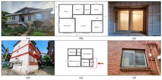
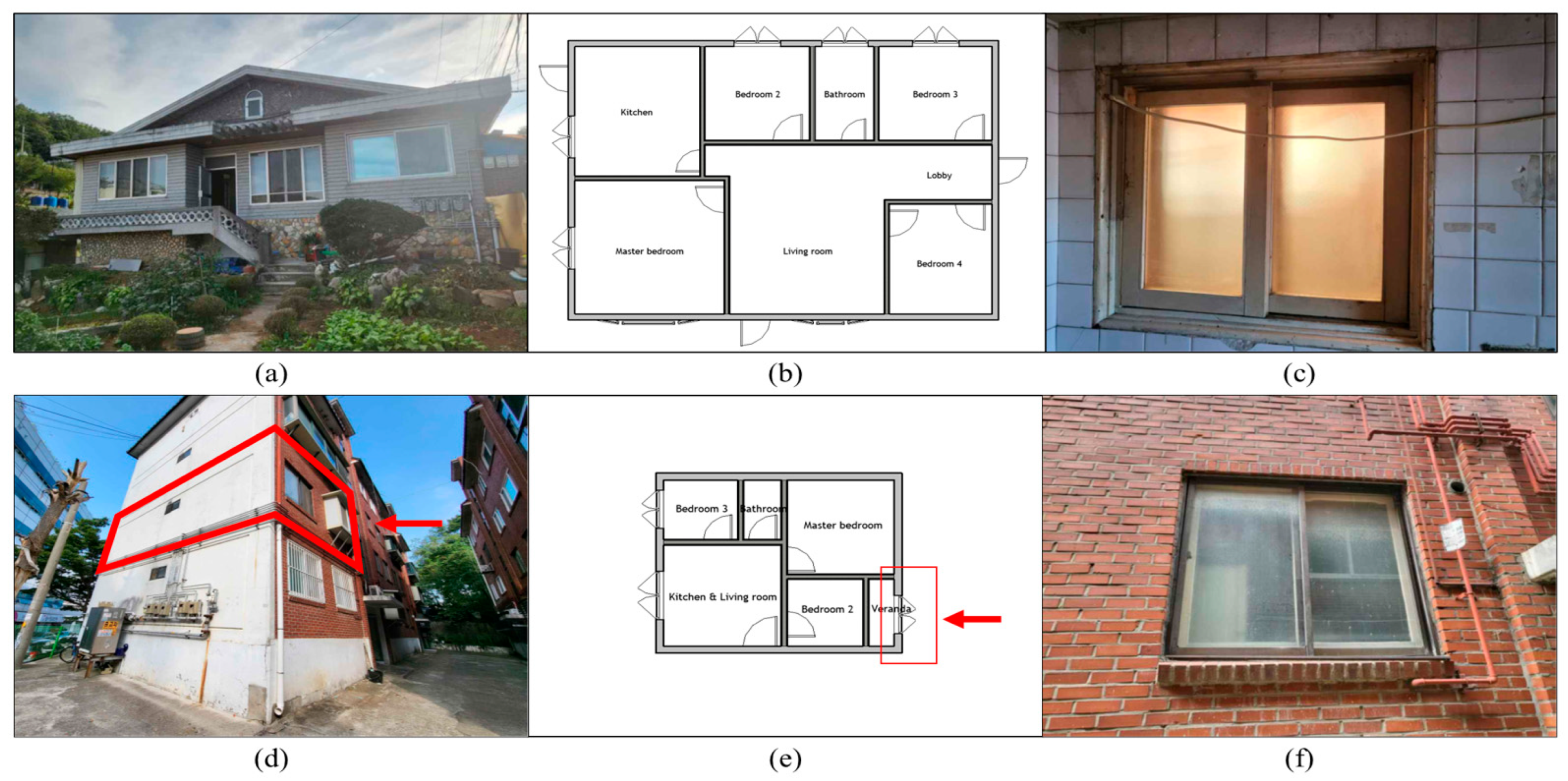
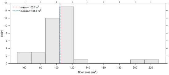
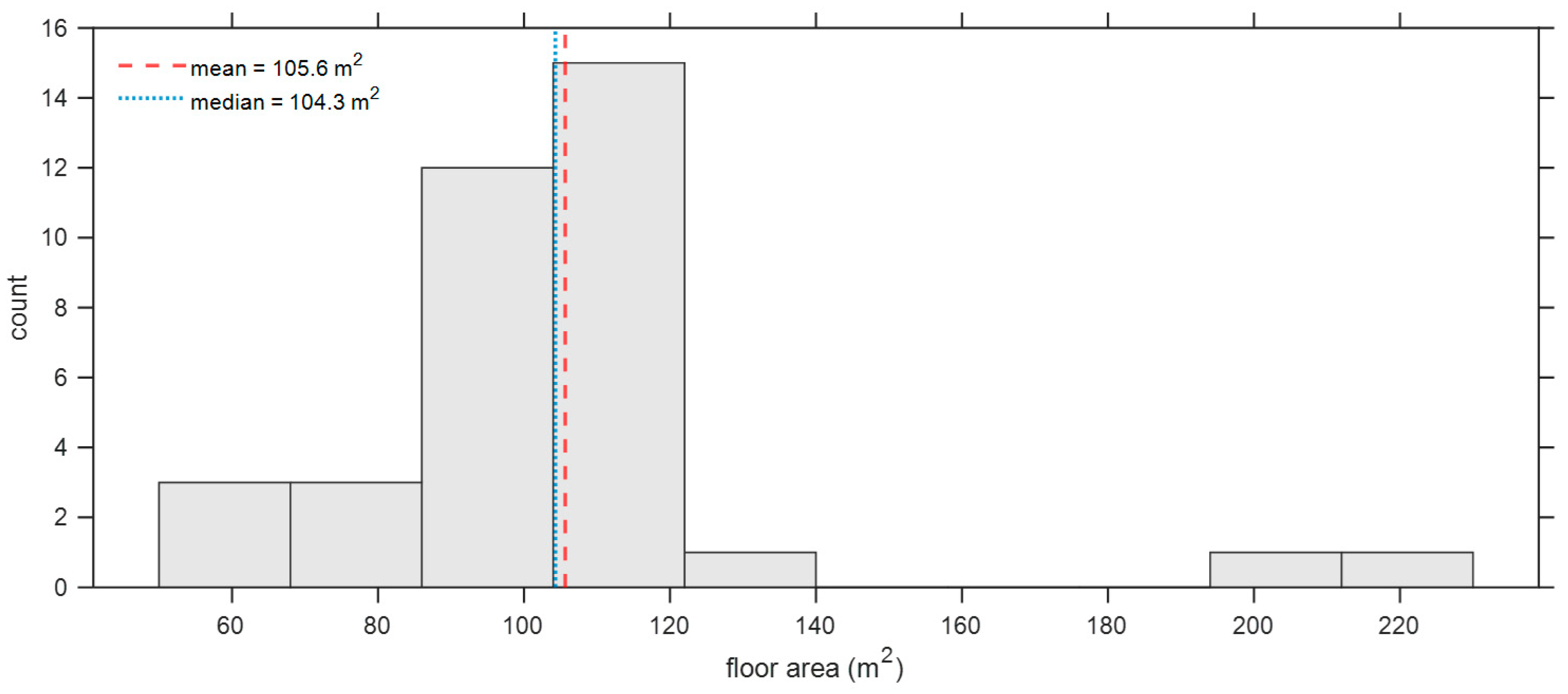
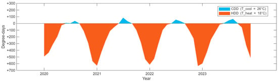
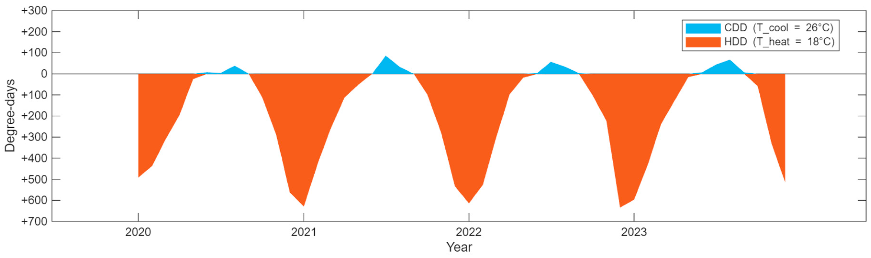
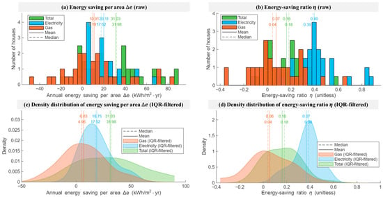
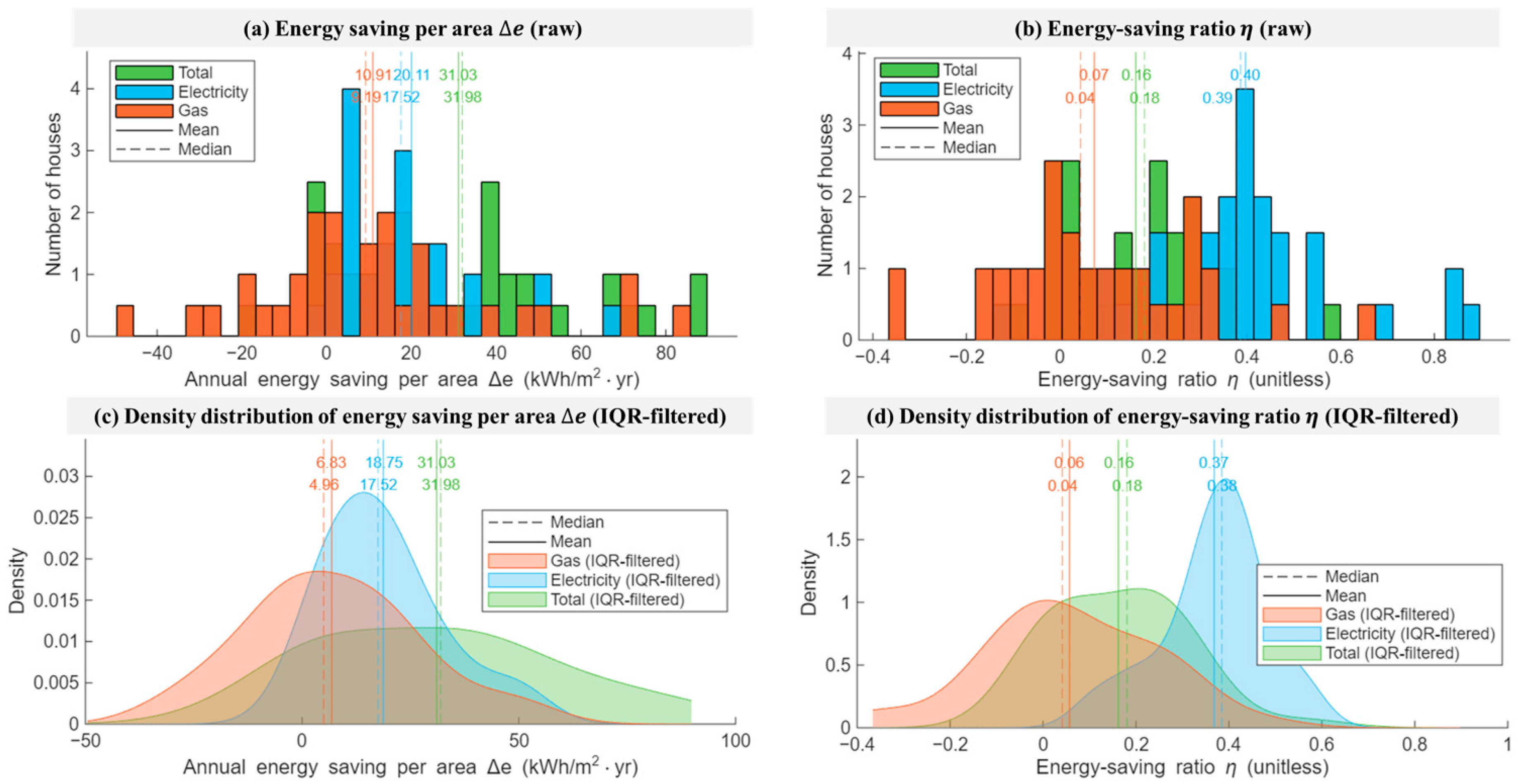
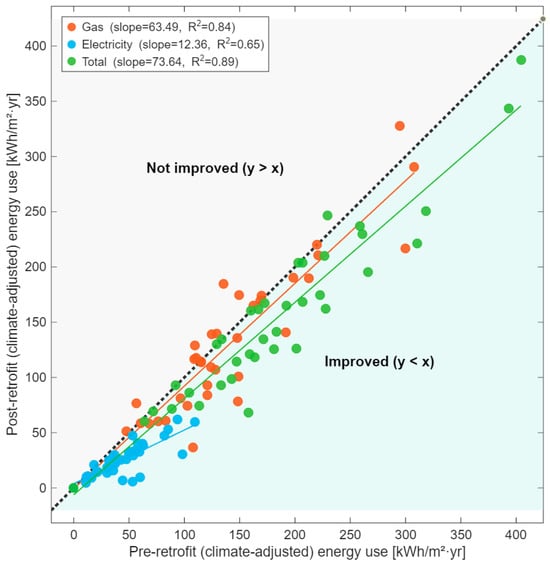
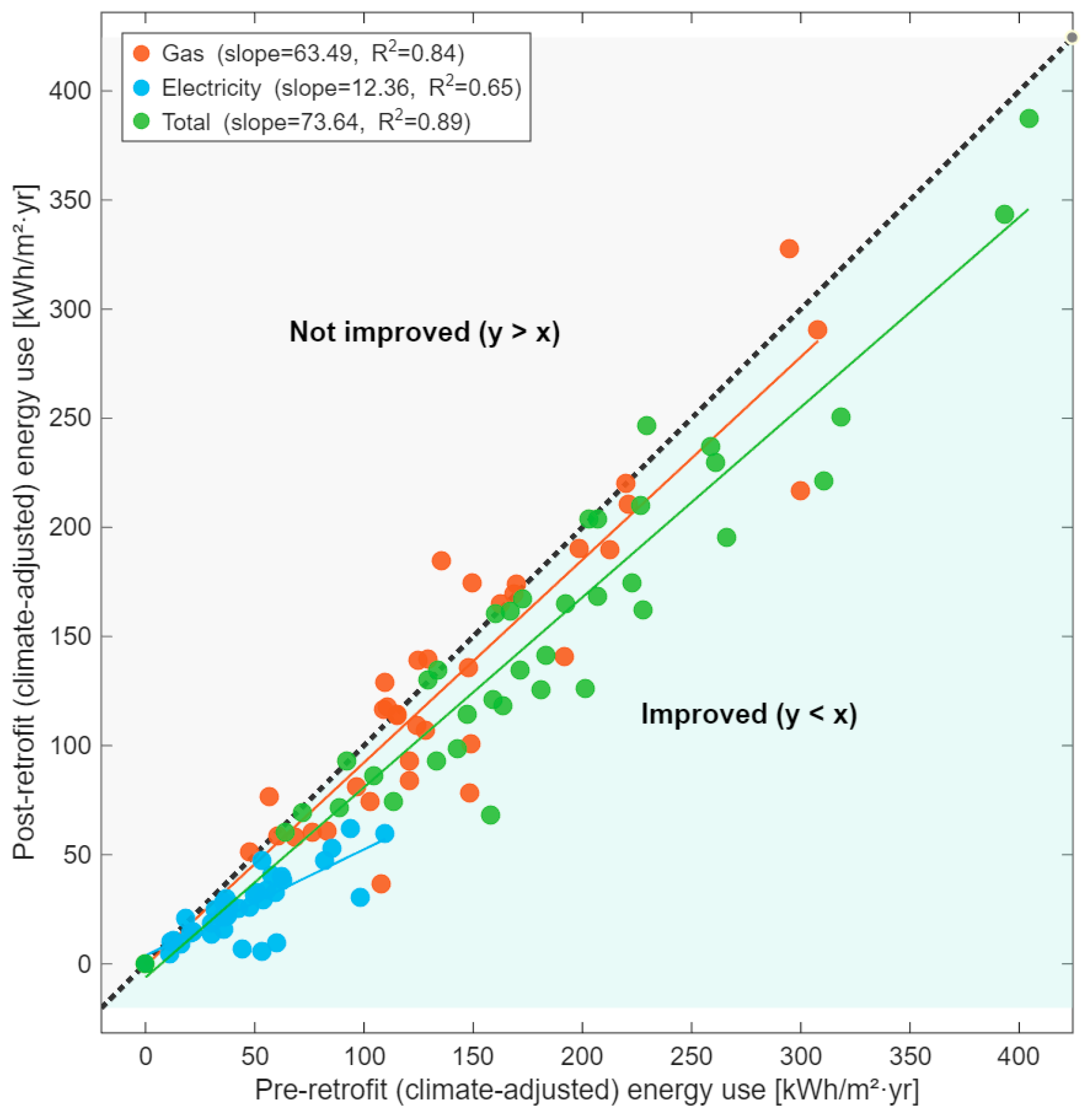
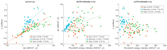
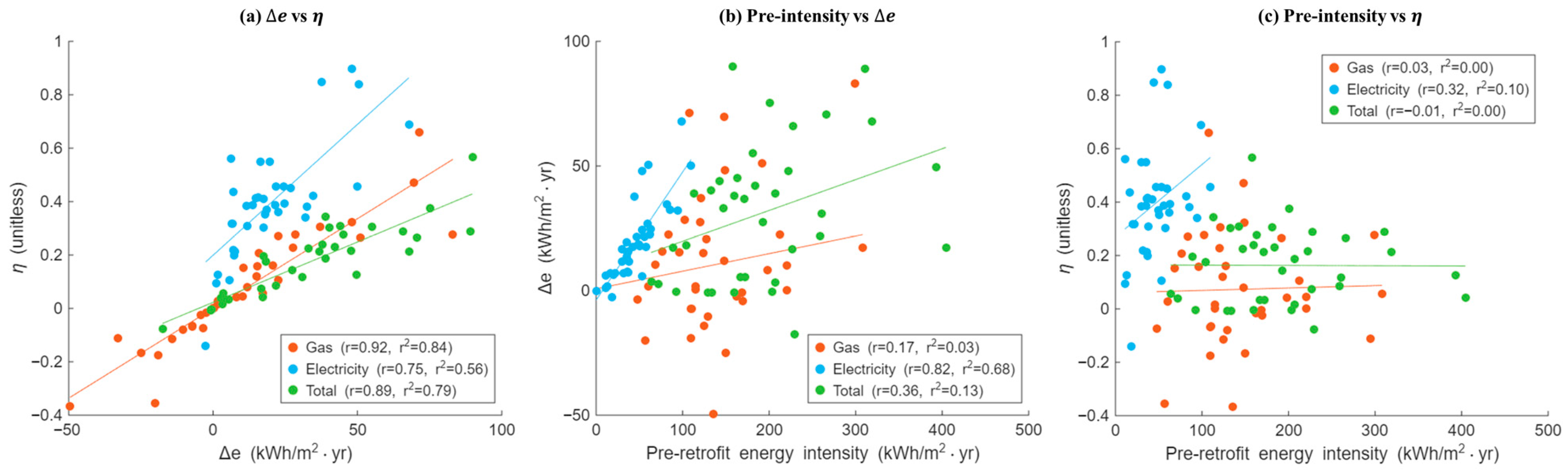
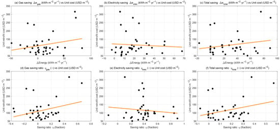
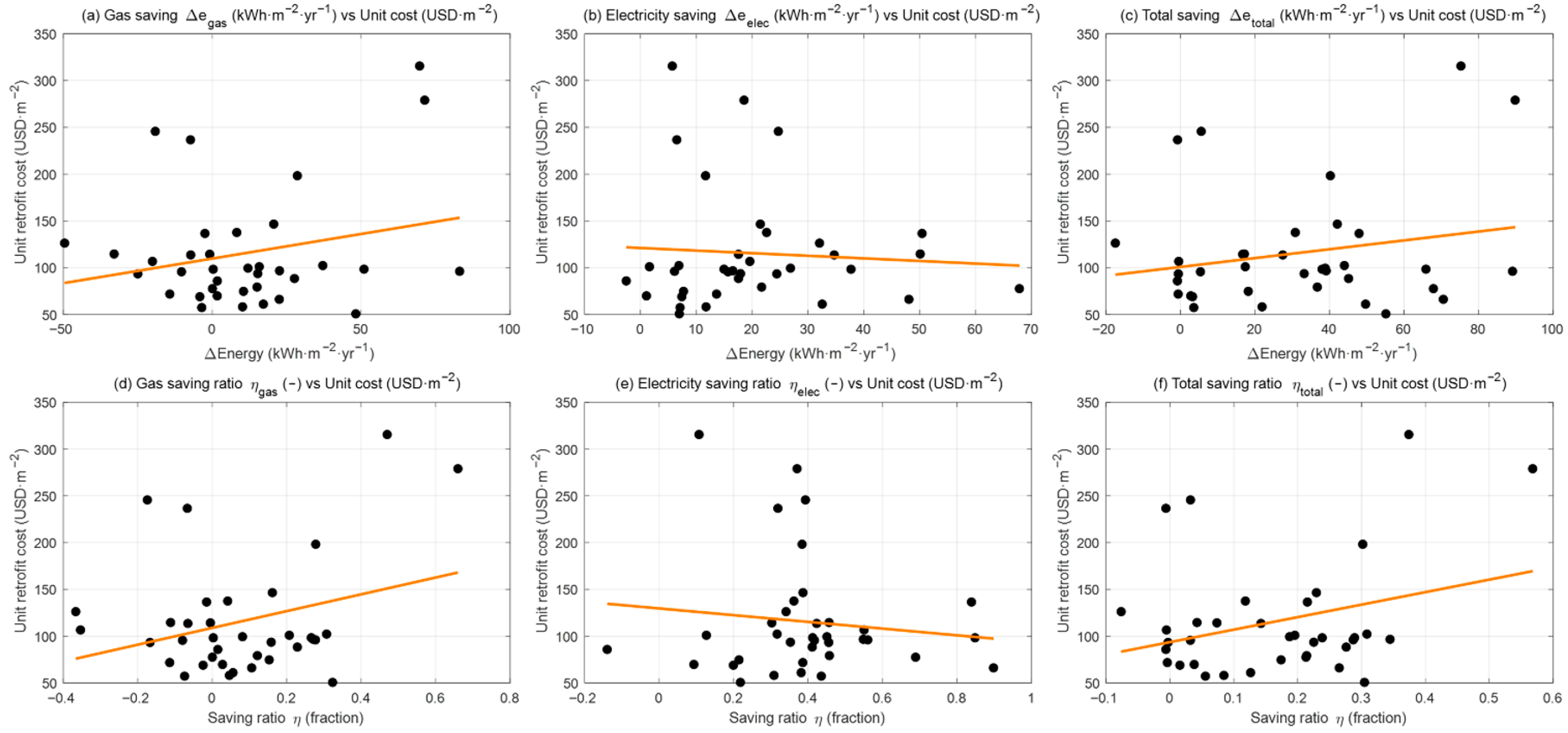
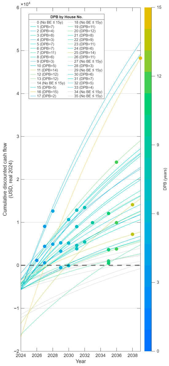
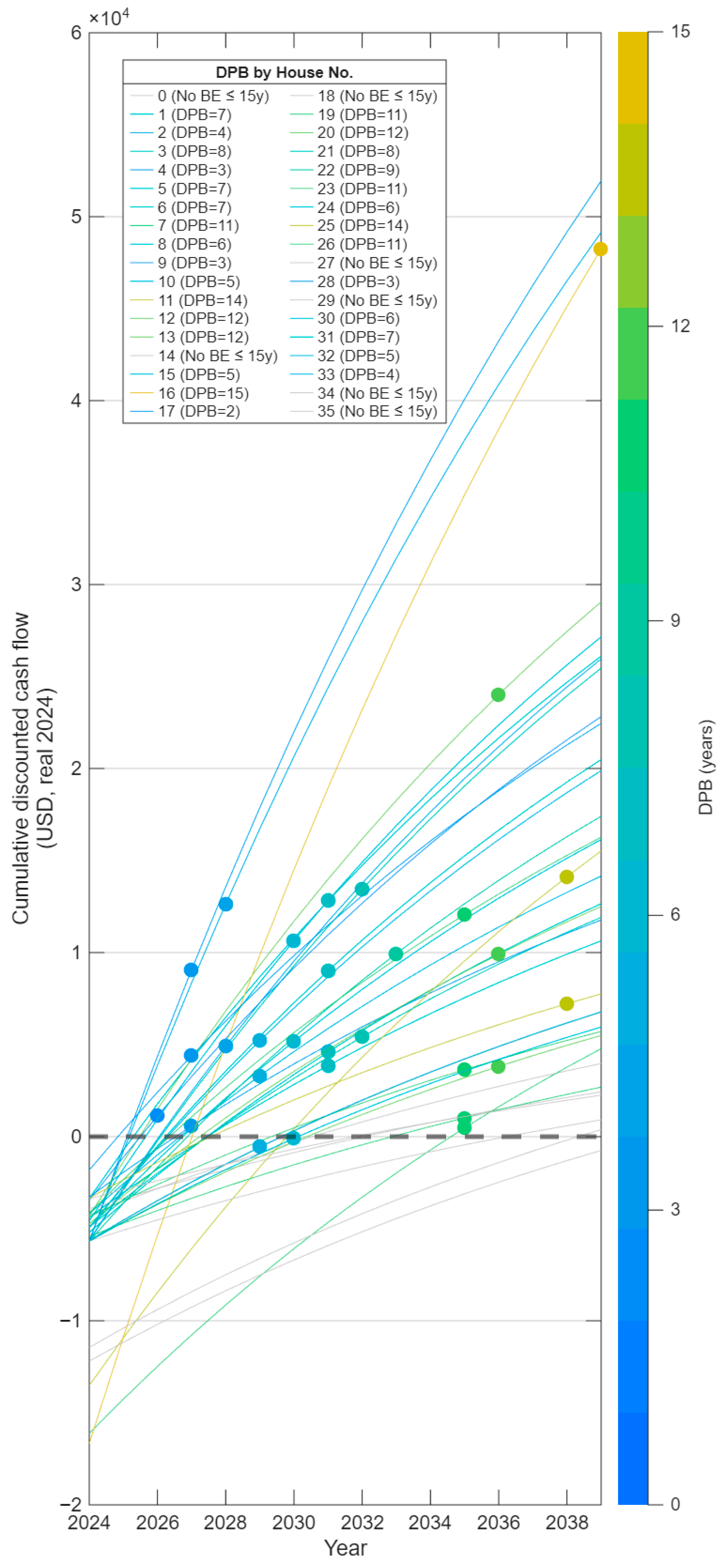
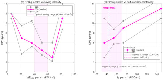
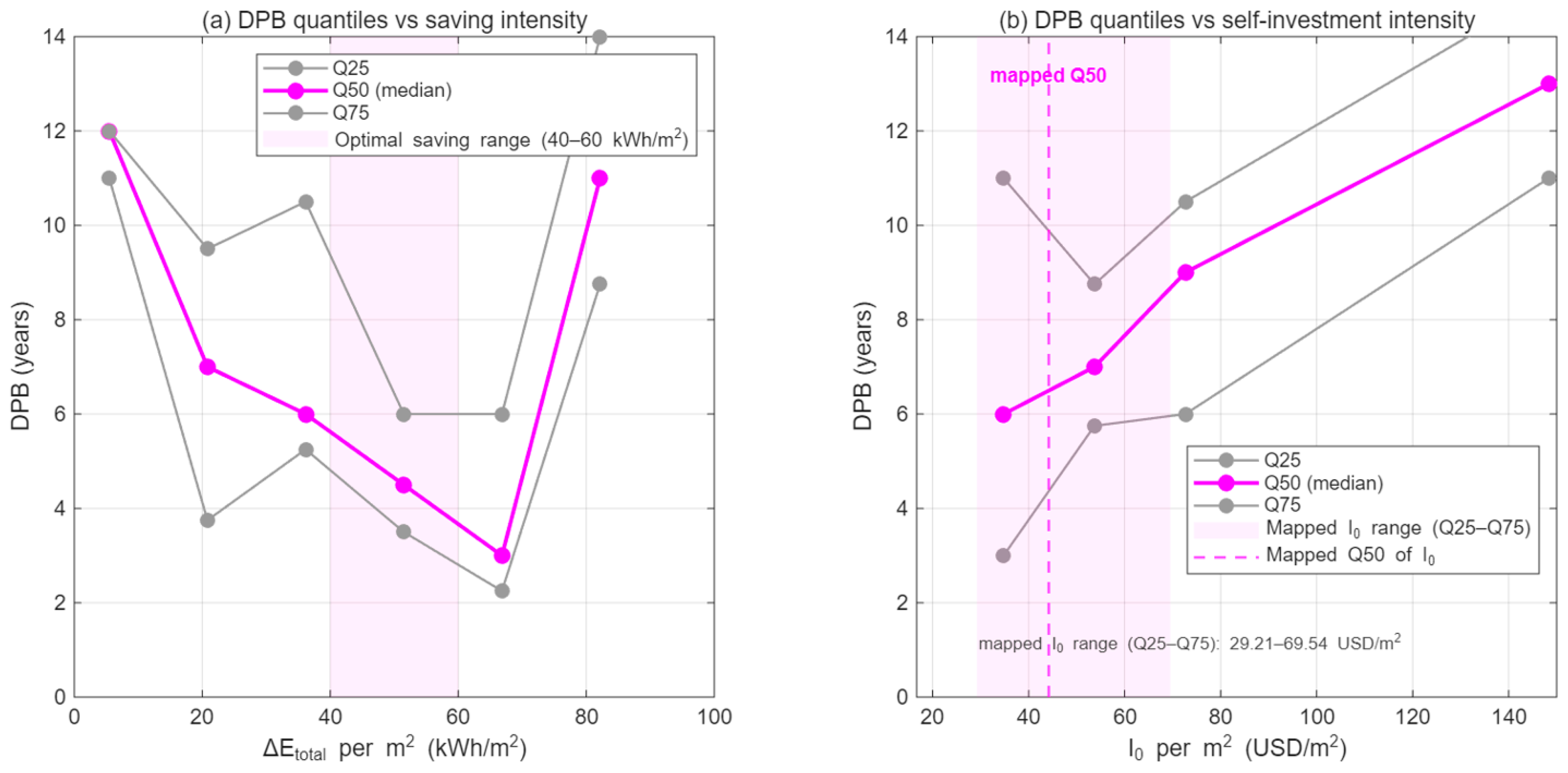
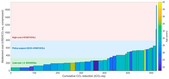
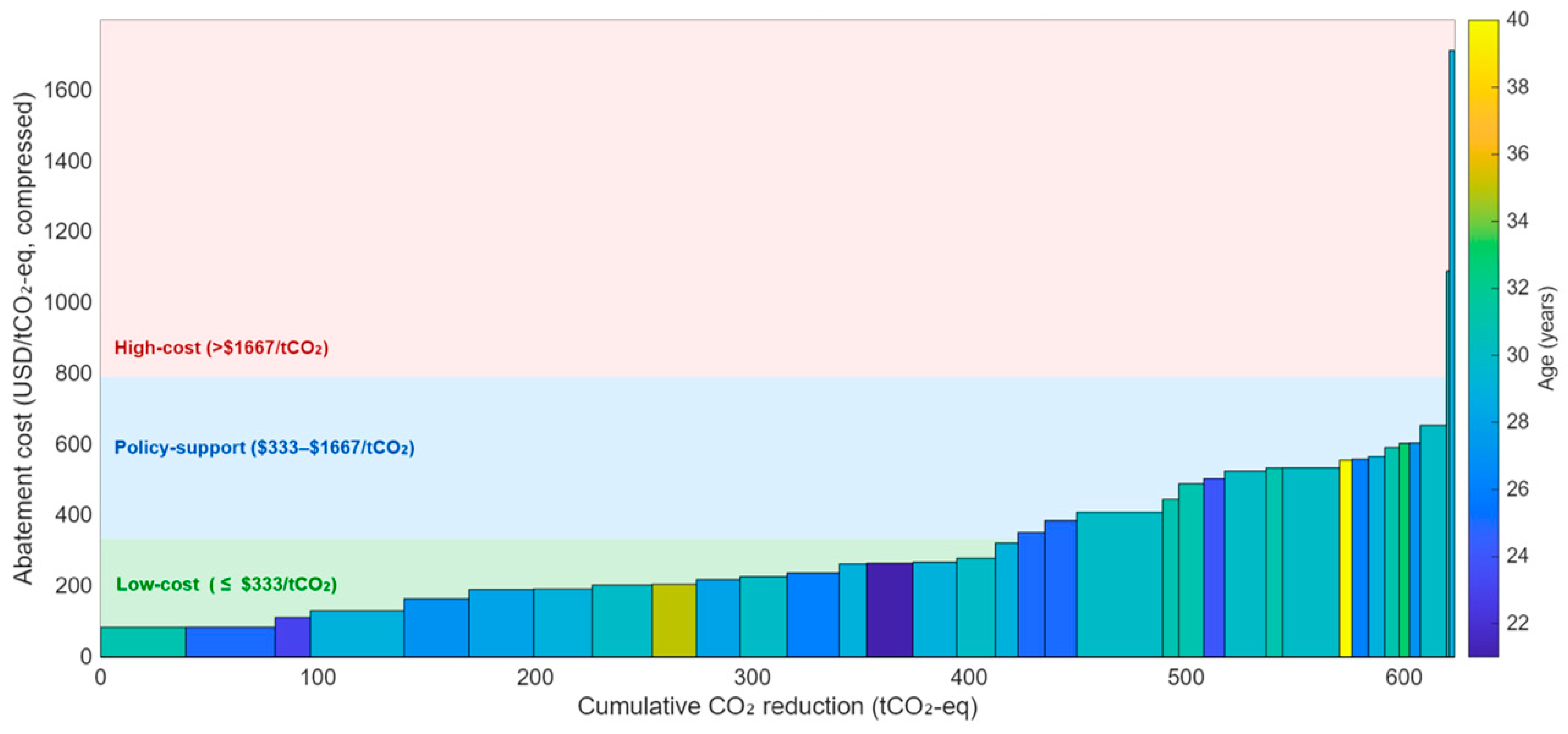
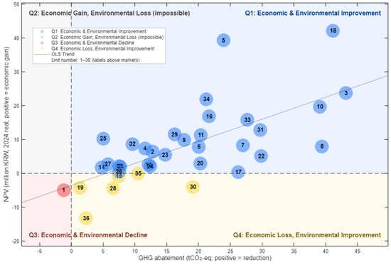
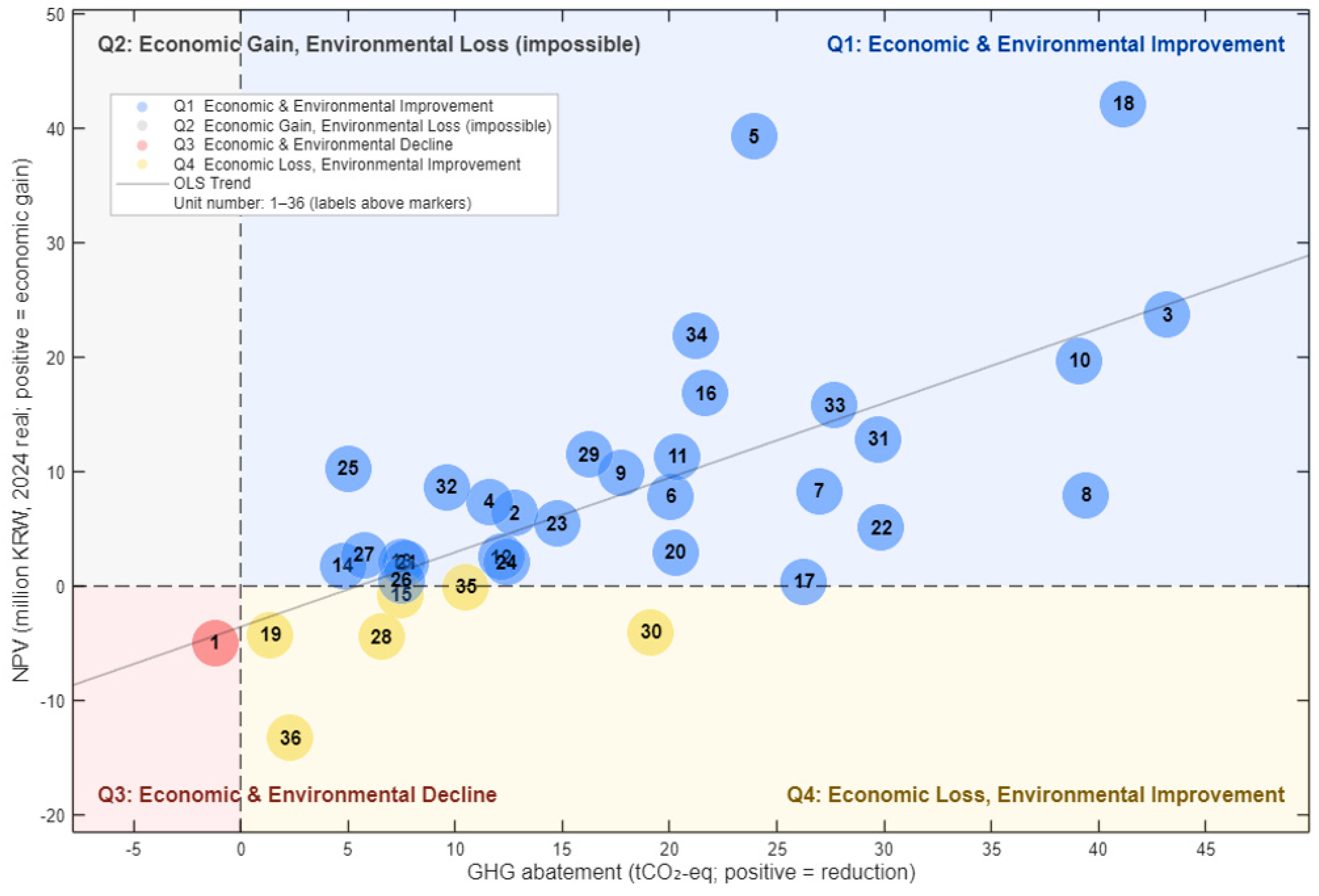
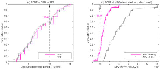
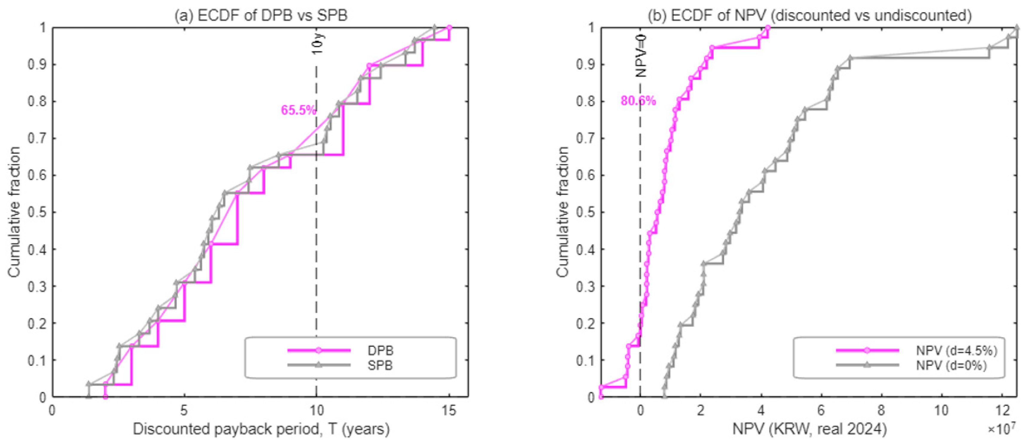
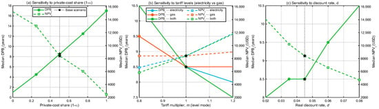
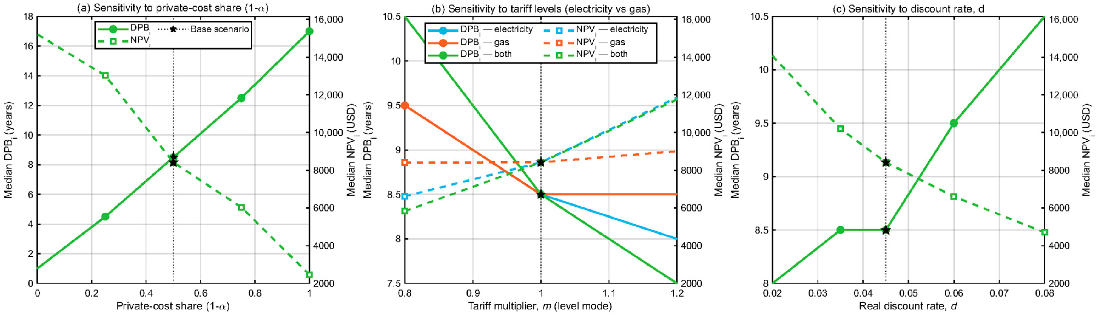

Disclaimer/Publisher’s Note: The statements, opinions and data contained in all publications are solely those of the individual author(s) and contributor(s) and not of MDPI and/or the editor(s). MDPI and/or the editor(s) disclaim responsibility for any injury to people or property resulting from any ideas, methods, instructions or products referred to in the content. |
© 2025 by the authors. Licensee MDPI, Basel, Switzerland. This article is an open access article distributed under the terms and conditions of the Creative Commons Attribution (CC BY) license.