Experimental and Machine Learning-Based Investigation of Coarse Aggregate Characteristics Impact on Mechanical Properties of Concrete

Abstract

This research investigates the impact of coarse aggregate (CA) type, shape, and specimen size on the compressive behavior of concrete, aiming to better understand how these factors affect its mechanical performance. Eight concrete mixtures were designed according to four different concrete mix design (CMD) codes using two types of coarse aggregates: crushed basalt and naturally rounded, both with a 15 mm size. A total of 96 concrete samples were tested to evaluate their failure mode, compressive strength (CS), energy accumulation (G_A), and post-peak fracture energy (G_F). The results show that concrete made with basalt CA offered significantly higher CS (by 7% to 40%), G_A (by 34% to 57%), and G_F (10% to 48%) compared to concrete made with natural CA across different CMD codes and specimen dimensions. Larger cylinders demonstrated higher CS than smaller cylinders, ranging from 7% to 19%. The incorporation of basalt CA enhanced the toughness and ductility of concrete, leading to superior post-peak behavior. In addition to the experimental program, four machine learning algorithms, i.e., Extreme Gradient Boosting (XGB), Gradient-Enhanced Regression Tree (GBR), Random Forest (RF), and Support Vector Regression (SVR), were employed to forecast the concrete’s CS. RF (R² = 0.93) and gradient boosting models (R² = 0.92) showed remarkable accuracy, whereas SVR underperformed. The feature importance and SHAP analysis identified cement content and CA type as the primary determinants of CS, while the water–cement ratio served as a crucial regulator. Moreover, a graphical user interface tool was developed to practically allow engineers to rapidly estimate concrete CS, bridging the gap between experimental validation and practical use.

1. Introduction

The impact of CA characteristics on the compressive behavior of concrete is critical and needs extensive investigation. In the construction industry, the diverse utilization of CA is essential for enhancing load-bearing capability, extending structural longevity, and controlling damage. Coarse aggregates constitute 60–75% of the concrete volume, making their role in the concrete mix fundamental to mechanical properties, such as CS, durability, and fracture energy (G_F) [1]. Research has indicated that while CA size slightly affects the CS of concrete [2], the type and shape of CA significantly influence CS. Moreover, fracture hardness and G_F were observed to be based on aggregate type and shape and to be independent of aggregate and specimen scale [3,4,5,6,7,8]. In contrary, another study found that the G_F of concrete enhanced as the CS and CA size increased [9]. Some studies have revealed that concrete with basalt CA provides superior CS and G_F compared with granite, limestone, and river gravel [10,11,12,13,14]. It was also reported that the fracture zone length and G_F of concrete are persistent and independent of the shape and size of the specimen [15]. These findings emphasize the importance of CA characteristics in optimizing concrete mechanical performance, providing a baseline for further research in this area.

Previous studies have reported the influence of CA types, shapes, and sources on the mechanical properties of concrete such as CS, modulus of elasticity (E_c), and energy dissipation. Research has demonstrated that concrete made with crushed CA exhibits higher E_c compared to concrete with spherical aggregates. Additionally, the G_F of concrete with crushed CA is marginally higher as the aggregate size increases [16]. Basalt CA has been shown to enhance the strength and permeability properties of concrete [17]. Comparison of different types and shapes of coarse aggregates were made and found that uncrushed and crushed CA provide comparable CS, thus arguing that uncrushed gravel can be a cost-effective choice for medium-strength concrete [18,19]. Concrete produced with quartzite CA has been illustrated to achieve higher CS compared to those made with natural river and granite coarse aggregates [20]. The influence of concrete type and maximum CA size on compressive properties indicates that while the effect of CA size on CS is minimal, the impact increases as the unit weight of the concrete decreases [21]. The type, internal composition, and surface characteristics of crushed granite, washed gravel, and unwashed gravel have been found to significantly affect CS. Notably, crushed granite CA has been found to yield the highest CS [22]. Moreover, the CS of concrete improves with a reduction in the water-to-cement (W/C) ratio, particularly when crushed CA is used [23]. Further studies have shown that increasing the volume fraction of coarse aggregates enhances both E_c and CS of concrete [24]. Additionally, incorporating basalt CA with plasticizers can substantially increase the compressive properties of concrete [25,26].

The surface properties of CA also play an important role in the strength characteristics of concrete. A detailed assessment was carried out considering the impact of various CA types on the mechanical properties of concrete, i.e., CS, tension, and E_c. The compressive property of high-strength concrete (HSC) is said to be affected by CA type but unaffected in the case of normal-strength concrete (NSC). Tensile intensity is often unaffected by aggregate type, although CA surface properties influence it [27]. Research has indicated that concrete made with crushed granite achieves higher CS than that made with natural CA [28]. In contrast, uncrushed coarse aggregates are recommended for medium-strength concrete due to their superior compressive, flexural, and splitting tensile strengths compared with crushed aggregates [29]. Quartzite CA exhibits superior performance in terms of CS among different CA types, such as granite and river gravel [30]. The type of CA significantly influences the CS and G_F of HSC more than NSC [31]. Furthermore, the source of CA also affects concrete strength, with natural aggregates generally outperforming recycled aggregates, although their CS was comparable [32,33,34]. The shape of the CA and varying W/C ratios influence the workability and compressive and tensile strengths of concrete. It was found that CA shape had little effect on concrete workability but substantially impacted concrete CS. Furthermore, higher CS has been reported in concrete with a smaller proportion of flaky and elongated CA [35,36]. CA type has a major impact on concrete CS and E_c but a minor impact on tensile and flexural strengths [37,38]. The morphological features of CA, such as flatness, angularity, and rigidity, are critical factors influencing the rheological and mechanical properties of fresh concrete [39]. Overall, the selection of CA type, shape, and source is crucial for optimizing the mechanical performance of concrete.

In addition to the effect of CA characteristics, CMD is crucial for selecting materials and their precise proportions to produce economically feasible concrete with specific properties [40,41]. Over the past few decades, researchers have focused on optimizing CMD to enhance mechanical properties at low cost. Various studies have meticulously regulated concrete proportions to evaluate the impact of different aggregate compositions on concrete quality [42]. Factors such as the maximum CA size, sand ratio, and W/C ratio have been experimentally investigated in order to analyze the density, CS, and E_C of concrete [43]. Comparative studies have assessed different CMD guidelines, highlighting variances in concrete ingredient content, strength properties, and cost [44,45]. The British and American standard CMD codes have been examined using crushed and uncrushed CA. Differences in workability and cost were reported, although both codes provided sufficient CS [46,47]. Additionally, studies have outlined the principles of various CMD methodologies concerning quality, cost-effectiveness, and exposure conditions, observing necessary adjustments for quality and cost control [48,49]. Environmental considerations in concrete production highlight that cement is the primary source of environmental impact, contributing approximately 75–90% of the carbon footprint, with sand, gravel, and admixtures also impacting life cycle assessment [50,51]. Moreover, the World Business Council for Sustainable Development reported that the manufacturing of ordinary Portland cement (OPC) produces an average of 842 kg CO₂/t of clinker [52]. These findings underscore the need for comprehensive CMD approaches that address mechanical performance, cost-effectiveness, and environmental concerns.

Modern infrastructure development relies heavily on concrete. In addition to guaranteeing structural integrity, precise predictions of its mechanical characteristics also help optimize material use, minimize environmental impact, i.e., the carbon footprint associated with cement production, and increase the effectiveness of CMD [53]. In the past, empirical methods were employed to estimate concrete qualities owing to their simplicity and dependence on observable factors like W/C ratio and aggregate size. However, when applied to a variety of material compositions, these methods often produce less accurate predictions with poor generalizability due to their inability to capture the intricate and nonlinear interactions among the heterogeneous components of concrete and its properties [54]. Considering the limitations of conventional approaches in addressing such intricacies, machine learning (ML) techniques have surfaced as strong options. ML models, especially ensemble approaches such as Random Forest (RF) and gradient boosting models, have become increasingly popular for their enhanced generalizability and accuracy, making them ideal for handling complicated data and producing reliable predictions [55].

The use of several ML techniques to forecast the mechanical properties of concrete has been systematically examined [56]. Several studies employed different ML techniques to forecast the strength properties of concrete including RF, support vector machine (SVM), gradient boosting models, artificial neural networks (ANNs), and decision trees [57,58,59,60,61,62]. Furthermore, deep learning approaches have played a crucial role in enhancing predictive modeling. Convolutional neural networks (CNNs) and ANNs are particularly efficient for identifying intricate patterns and processing large datasets, rendering them highly effective for predicting concrete mechanical properties [63,64,65,66]. Concrete mechanical properties prediction has also benefited from the effective use of evolutionary algorithms [67], such as gene expression programming, which has the advantage of producing interpretable models with empirical equations that are useful in certain applications. The advancement of ML, deep learning, and evolutionary techniques has significantly improved our understanding of concrete’s mechanical behavior, enabling more accurate and efficient predictions for modern construction, including optimizing CMD, enhancing material sustainability, and project efficiency.

In summary, the impact of CA type, specimen geometry, or CMD technique has usually been studied separately in previous research [2,9,12,14,16,17,18,19,20,21,22,23,24,25,26,31,32,33,34,35,36]. However, all of these aspects can have a combined impact on real-world concrete applications, and their interactions are still partially understood. Furthermore, ML models have rarely been used in conjunction with controlled experimental research that take into account changes in CMD codes and specimen configurations at the same time. The current study closes this gap by conducting a comprehensive experimental and ML-based assessment of concrete mixtures prepared according to four distinct CMD codes (ACI, BS, IS, and JGJ), using two types of CA (crushed basalt and naturally rounded) and several specimen dimensions to evaluate their impacts on the overall compressive behavior of concrete.

Building on the experimental results, ML models (XGB, GBR, RF, and SVR) were developed and employed to (i) accurately predict 28-day CS and (ii) clarify mechanistic mix variables through feature importance analysis. Ultimately, the study concludes with the development of a practical streamlined graphical user interface tool that facilitates rapid, mix-aware strength estimation for both design and quality control purposes. This integrated experimental–ML system offers new insights for research and real-world concrete design, as it is the first to jointly integrate different CMD codes, CA types, specimen sizes, and ML models’ predictions into a single comparative framework.

2. Experimental Framework

An experimental framework was developed to evaluate the impact of CA type, shape, and specimen size on the compressive behavior of NSC. A total of eight concrete mixtures were prepared according to four different CMD guidelines. The concrete mixtures were made with crushed basalt CA and naturally rounded CA, both with a maximum size of 15 mm. The concrete samples were cured for 28 days and tested under axial compression in displacement-control mode. Furthermore, ML techniques were developed, and their precision ability was assessed using the experimental and relevant literature data.

2.1. Materials

Ordinary Portland cement with a grade strength of 42.5 MPa, as specified in the Chinese standard GB175-2007 [68], and a specific gravity of 3.15, was utilized as the binder. The fine aggregate was river sand with a specific gravity of 2.4, water absorption of 0.89%, fineness modulus of 2.22, and moisture content of 1.07%. To determine the nature of sand and CA, testing was performed by following Equations (1)–(4) of the IS:2383 [69]. Basalt CA with a specific gravity of 2.7, water absorption of 1.1%, and natural CA with a specific gravity of 2.54 and water absorption of 0.56% were used. To obtain the exact CA size of 15 mm, a sieving process was performed. The classification of CA was based on their well-established geological sources. Basalt CA was characterized as angular in shape and mechanically crushed, while naturally occurring river CA was delivered with a smooth surface and rounded shape. Tap water available in the laboratory was used for concrete batching and curing.

$$\mathrm{Specific} \mathrm{gravity} \mathrm{of} \mathrm{FA} S_G={\displaystyle \frac{D}{A-\left(B-C\right)}}$$

(1)

$$\mathrm{Water} \mathrm{absorption}\% W_{abs}={\displaystyle \frac{\left(C-D\right)}{D}}\times 100$$

(2)

$$\mathrm{Moisture} \mathrm{content}\% P_{mc}={\displaystyle \frac{V_s-V_d}{M_s-V_s}}\times 100$$

(3)

$$\mathrm{Specific} \mathrm{gravity} \mathrm{of} \mathrm{CA} S_G={\displaystyle \frac{D}{C-\left(A-B\right)}}$$

(4)

In Equations (1) and (2), S_G = specific gravity, W_abs = water absorption, A = weight in g of the saturated surface-dry sample, B = weight in g of the pycnometer containing the sample and filled with distilled water, C = weight in g of the pycnometer filled with only distilled water, and D = weight in g of the oven-dried sample. In Equation (3), P_mc = moisture content, Vs = weight in g of water displaced, V_d = weight of the dry sample, M_S = weight in g of the sample. In Equation (4), A = weight in g of the vessel containing the sample and filled with distilled water, B = weight in g of the vessel filled with distilled water only, C = weight in g of the saturated surface-dry sample, and D = weight in g of the oven-dried sample.

2.2. Concrete Mix Design Codes

The goal of the CMD is to proportion the ingredients to produce durable concrete that satisfies the strength requirements at the lowest possible cost. For this reason, many countries have developed CMD codes based on the exposure requirements and the nature of the materials readily available in the region. In this study, the following four CMD codes were evaluated: the American Concrete Institute (ACI) code [70], the British (BS) code [71], the Indian (IS) code [72,73], and the Chinese (JGJ) code [74]. ACI, BS, IS, and JGJ are the acronyms used for the mentioned CMD codes. These CMD codes adopt different design methodologies, including empirical proportioning. These CMD codes were selected to reflect commonly used regional practices across different countries of the world and to evaluate performance differences in fresh and hardened concrete properties concerning aggregate type and ingredient proportioning methodologies. Concrete mixtures with a design strength of 25 MPa were proportioned according to the four CMD codes, respectively. Figure 1 shows the concrete mixtures prepared with basalt CA and natural CA. There are noticeable variations in the quantity of concrete components stated in these CMD regulations for NSC. For basalt CA, the BS code used the highest cement content, followed by IS, ACI, and JGJ. The highest water content was utilized by BS and JGJ, followed by ACI and IS codes. ACI had the highest sand content, whereas JGJ had a lower quantity of sand. There was virtually no difference between the IS and BS codes in terms of the quantity of sand. The largest amount of CA was used by BS, followed by IS, JGJ, and ACI. In the case of natural CA, the IS and BS codes had the highest cement concentration, followed by ACI and JGJ codes. The highest water content and sand content were used by ACI, followed by BS, JGJ, and IS codes. Compared with the other codes, BS had the highest CA content.

2.3. Specimen Preparation and Testing Procedure

A gravity-type rotating mixer was used to blend the concrete ingredients. Before the batching phase, the ingredients were weighed. The inner surface of the mixer was cleaned before pouring the concrete ingredients to ensure that the required amount of water was used to hydrate the cementitious content, which is a key aspect. The concrete ingredients were placed into the mixer pan in sequence, i.e., sand and CA were first added and dry-mixed for one minute, then cement was added and further mixed for another one minute. After the dry-mixing process, approximately 70% of the water was introduced and mixed for the next two minutes. The remaining water content was then added, and mixing of concrete ingredients continued for the next two minutes until a uniform mixture was formed. The ASTM C192/C192M-16 [75] standard was followed to prepare and cure the concrete samples. Concrete was poured into plastic molds and compacted using a vibrator machine to eliminate entrapped air. The concrete specimens were demolded after 24 h and placed in water tanks at 28 ± 2 °C for a 28-day curing period. During curing, the humidity was maintained at approximately 70–80%. The curing water was replaced every seven days to maintain proper curing conditions and stable temperature. After curing process, the top and bottom ends of all samples were ground to ensure consistent load distribution during testing. This program encompassed a total of 96 concrete samples, comprising three distinct geometries, i.e., 32 cubes of size 150 × 150 × 150 (mm), 32 large cylinders with dimensions of 150 mm diameter and 300 mm height, and 32 small cylinders measuring 100 mm in diameter and 200 mm in height. The specimen surfaces were cleaned and labeled with specific numbers before testing to prevent inconvenience during testing. Figure 2a shows the specimen configurations.

To measure the workability of concrete mixtures, slump tests were performed immediately, as the concrete mixtures were prepared in accordance with ASTM C143/C143M-15a [76]. Axial compression testing was conducted following the ASTM C39/C39M-15 [77]. A universal compression test machine with a capacity of 1000 MPa was used to measure the CS of the concrete cubes at a loading rate of 0.3 MPa/s. The cylinders were loaded at a steady rate of 0.3 mm/min in displacement-control mode. A 1000 kN servo-hydraulic machine was used to test the cylindrical specimens with a load drop of 100 kN/m². The testing machine was calibrated within ±1.0 accuracy as per laboratory technician instructions. To measure deformation, two vertical and two horizontal strain gauges of 60 mm were attached at mid-height, i.e., at 150 mm and 100 mm marks from the top of the large and small cylinders, respectively. The specified areas for strain gauges installation were prepared using the appropriate sandpaper and cleaned with a solvent (acetone). The strain gauges were attached using locally available instant adhesive. Figure 2b,c depict the testing setup.

3. Machine Learning Applications

This research further investigates the use of four ML models, i.e., Extreme Gradient Boosting (XGB), Gradient-Enhanced Regression Tree (GBR), Support Vector Regression (SVR), and Random Forest (RF), to validate the experimental program and predict the CS of concrete. These models were chosen because of their strong applicability over a range of datasets, high-dimensional dataset management, and handling of nonlinear interactions. To enhance prediction accuracy, XGB and GBR utilize boosting methods for iterative error correction, whereas RF relies on an ensemble of decision trees to mitigate overfitting and enhance robustness. In contrast, SVR employs a margin-based regression technique that performs well in high-dimensional domains. These models provide a complete toolset for solving a variety of regression problems in engineering and scientific applications.

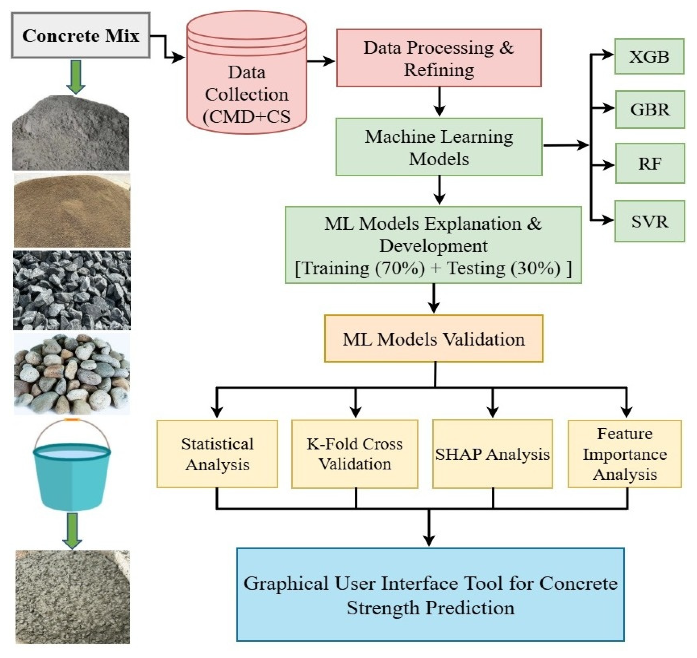
For the ML models, the CS values of a 28-day curing period were computed. The preliminary dataset was established using experimental data and data from 14 relevant existing studies [9,14,23,28,29,30,32,34,35,38,45,47,49,78]. To maintain uniformity with the experimental practice, only mixtures that corresponded to NSC, i.e., 20 MPa–36 MPa, were considered. The data of various geometrical concrete specimens, including standard cubes, small cylinders (100 × 200 mm), and large cylinders (150 × 300 mm), were organized, and the 28-day CS values were normalized using frequently adopted conversion relationships. This method guaranteed that variations in specimen geometry did not lead to any bias in the ML model. An empirical relationship, $f_{CYL}=\alpha f_c$ (where $\alpha$ = conversion factor ranging from 0.78 to 0.85, depending on the concrete strength), was adopted to convert the CS of standard cubes to CS of large cylinders. This empirical relation of strength conversion from cube to cylinder is widely used [79,80]. In this study, conversion factors of 0.8 for cubes and 1.05 for small cylinders were adopted, which are suitable for NSC. Finally, a dataset containing 344 CS results with various CMD compositions was employed for the development of the ML models. The dataset was preprocessed by removing incomplete/missing entries, verifying consistent units for all mixture components, excluding unrealistic and inconsistent observations, and constructing the input–output structure. The dataset was divided in 70% (training) and 30% (testing). The output parameter was the 28-day CS, while the input variables were cement (kg/m³), water (kg/m³), sand (kg/m³), CA (kg/m³), W/C ratio, and CA type. An overview of the ML applications workflow is illustrated in Figure 3.

3.1. Machine Learning Algorithms Methodology

3.1.1. Extreme Gradient Boosting

Extreme Gradient Boosting (XGB) is an ensemble ML technique often used for classification and regression problems due to its high efficiency and scalability. This ML technique was designed to combine several trained models, enhancing predictive accuracy beyond what individual models can achieve. XGB, developed by Chen and Guestrin, is a cutting-edge ensemble technique for training gradient-boosted decision trees, notably proficient at modeling complex nonlinear interactions [81]. This implementation of gradient boosting incorporates several improvements to the conventional framework, including regularization, parallelization, and effective management of missing data. XGB employs decision trees as base learners and repeatedly improves its predictions by using gradient descent to optimize a loss function. These properties together enable XGB to develop predictive models with strong generalization capabilities. The combination of these qualities enables XGB to develop prediction models with strong generalization capabilities, which contributes to its extensive application in civil engineering for addressing complex modeling challenges [82,83]. XGB repeatedly adds trees to correct the mistakes of the previous ones, with a new decision tree being built in each iteration to minimize the residual errors from the prior trees. The objective function can be presented as in Equation (5).

$$\mathcal{L} \left(\varnothing \right)={{\displaystyle \sum }}_{i=1}^{n}l \left({\mathrm{y}}_i,{ŷ}_i\right)+{{\displaystyle \sum }}_{k=1}^K\mathsf{\Omega } {\mathsf{ƒ}}_k$$

(5)

where $l \left({\mathrm{y}}_i,{ŷ}_i\right)$ is the loss function that measures the error between the true value ${\mathrm{y}}_i$ and predicted value ${ŷ}_i$. $\mathsf{\Omega } \left({\mathsf{ƒ}}_k\right)$ is the regularization term that penalizes the complexity of the individual tree ${\mathsf{ƒ}}_k$. n is the number of samples, and K is the number of trees.

The regularization term plays a vital role in mitigating overfitting by imposing limitations on large or excessively complex trees. The most frequently employed regularization term is presented in Equation (6).

$$\Omega \left({\mathsf{ƒ}}_k\right)=\gamma T+{\displaystyle \frac{1}{2}}\lambda {\Vert {\mathsf{\omega }}_k\Vert }^2$$

(6)

where γ controls the complexity of trees, T indicates the number of leaves in trees, ω_k is the weight of the k-th leaf in the tree, and λ work as a regularization term to control the weight size.

The training procedure uses the Taylor expansion of the loss function and second-order gradient information to minimize this objective function. The outputs from each tree are added together to determine the final forecast when the boosting procedure is completed. The XGB model for concrete strength estimation can be presented as in Equation (7), where ${\mathsf{ƒ}}_k\left(x\right)$ is the result from the k-th tree.

$$F_{XGB}={{\displaystyle \sum }}_{k=1}^K{\mathsf{ƒ}}_k\left(x\right)$$

(7)

3.1.2. Gradient Boosting Regression

Gradient Boosting Regression (GBR), an ensemble approach, was suggested by Friedman in 2001 [84] for classification and regression. This technique is comparable to other boosting techniques. GBR combines many weak learners (decision trees) to create a powerful prediction model [85]. GBR functions in an iterative manner, training each weak learner using the prior model’s residuals. This allows subsequent models to enhance overall accuracy by tackling the limitations of their predecessors. Additionally, GBR uses a gradient descent optimization technique during training, in which the learning rate establishes the direction and size of model updates. Shrinkage rate tuning variables and n-trees are needed for GB regression, where n-trees represent the number of generated trees. The value of n-trees should not be minimal, and the learning rate, or shrinkage factor, applies to each expansion tree. The following Equations (8) and (9) present the GBR core function.

Training dataset of n samples $D={\left\{\left(x_i, y_i\right)\right\}}_{i=1}^n$, GBR model of M base learners, $h_m\in H$ (e.g., regression trees).

$$F_{M \left(x\right)}=F_0\left(x\right)+{{\displaystyle \sum }}_{m=1}^{M}v{\beta }_m{h}_m\left(x\right)$$

(8)

where $F_{M \left(x\right)}$ is the final predictor after M boosting iterations, $F_0\left(x\right)$ is the initial model, typically a constant to minimize the training loss, giving the first estimate before any trees are added. M is the number of boosting iterations (trees/weak learners). 0 < $v$ ≤ 1 is the shrinkage (learning rate). ${\beta }_m$ is a stage-specific scale (step size), and $h_m\left(x\right)$ is the base learner fitted at stage m (a shallow regression tree). Equation (8) represents the initial model.

$$F_0\left(x\right)=arg mi{n}_{\gamma \in R}{{\displaystyle \sum }}_{i=1}^{n}l\left(y_i,\gamma \right)$$

(9)

where $\gamma ={\displaystyle \frac{1}{n}} {\displaystyle \sum }_{i=1}^n{y}_i$  and $\gamma \in R$ is a constant parameter that minimizes the loss function $l\left(y_i,\gamma \right)$. l is a pointwise loss, e.g., squared error for regression, logistic loss for classification, and absolute error for robustness.

3.1.3. Random Forest

Random Forest (RF) is an ensemble learning technique that builds a multitude of decision trees during the training phase and produces the class label (for classification) or the mean prediction (for regression) from the individual trees. RF enhances decision trees by minimizing variance, thereby increasing the model’s resilience to overfitting. RF generates a collection of decision trees, each trained on a random subset of features and a random portion of training data, i.e., via bootstrapping. The first RF-based method was presented in 1995, followed by an enhanced version released by Breiman [86]. These algorithms have been widely used in many different fields and have shown exceptional performance, especially in tasks like classification and regression [87]. Regression is a statistical learning theory-based methodology that extracts multiple samples from the original data using the bootstrap resampling technique [88]. The RF method improves the variety of decision trees by allowing the use of replacement samples and including random changes in predictor combinations during the development of individual trees [89]. Equation (10) shows how the predictions generated by each tree are averaged to obtain the final outcome. 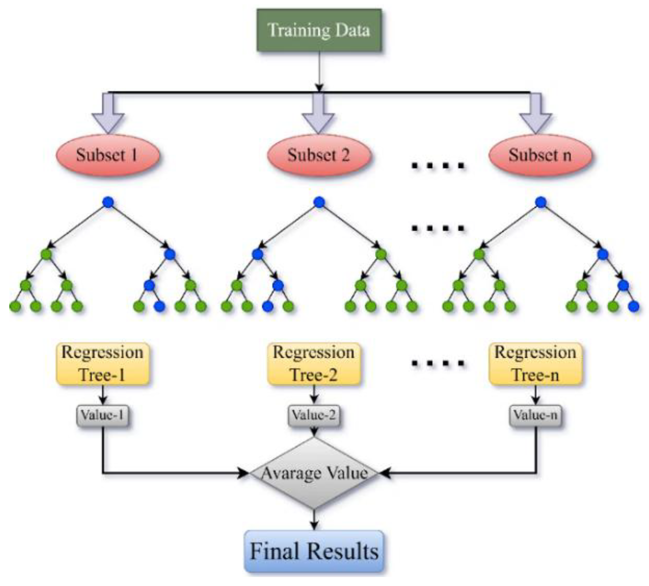Figure 4 presents a flowchart of the RF model, demonstrating the bootstrap sampling method to generate several data subsets, the construction of decision trees from each subset, and the aggregation of their projected values to obtain a final prediction outcome. In Figure 4, the blue circles represent decision nodes where the data is split based on features, while the green circles represent leaf nodes that provide the final predictions in the regression trees.

$$Ŷ={\displaystyle \frac{1}{T}}{{\displaystyle \sum }}_{t=1}^T{Ŷ}_i$$

(10)

where Ŷ is the final predicted result; T is the number of trees in the forest; Ŷi is the prediction from an individual tree (I = 1, 2, …, n), and n is the total number of trees.

3.1.4. Support Vector Regression

The support vector machine (SVM) technique was first developed by Vapnik [90] to solve classification problems, and it was later expanded to solve regression problems as well. The SVM method uses the Structural Risk Minimization (SRM) concept, which is more effective than the standard Empirical Risk Minimization (ERM) approach, according to research [91]. The SRM method works to lower a threshold on the predicted risk, whereas the ERM approach emphasizes the reduction in error concerning the training data. This differentiation provides SVM with an enhanced foundation for generalization, which is essential for statistical learning. Support Vector Regression (SVR) is a computational method that handle regression and prediction problems, based on SVM’s abilities [92]. A fundamental characteristic of SVR is its aim to reduce the training error observed during the learning process. Furthermore, SVR seeks to achieve performance that is applicable beyond the training data by minimizing the generalized error bound. In regression tasks utilizing SVM, the SVR is required to implement a cost function C to measure the empirical risk and subsequently minimize the regression error. Furthermore, the accuracy, complexity, and smoothness of the SVR approximation function are controlled by the epsilon-insensitive loss ε. A higher value of C and ε indicates a more complicated learning process for SVM [93]. 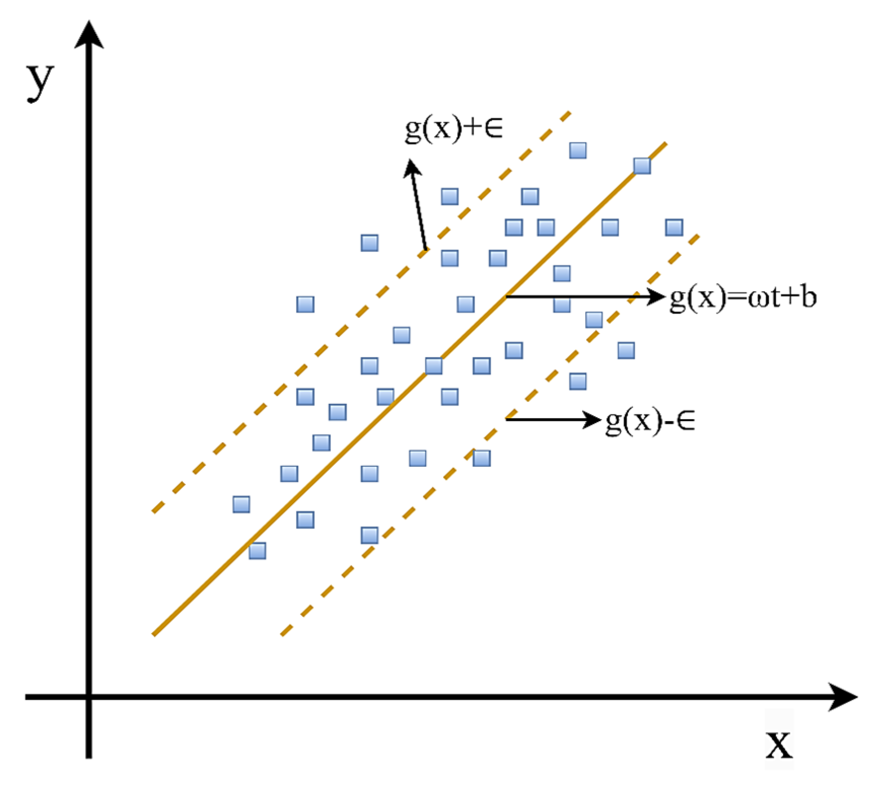Figure 5 illustrates the schematic representation of the SVR algorithm. The SVR optimization problem can be formulated by the subsequent Equations (11) and (12).

$$min{\displaystyle \frac{1}{2}}{\Vert \omega \Vert }^2+C{{\displaystyle \sum }}_{i=1}^{n}L \left(t_i,g\left(xi\right)\right)$$

(11)

$$\left\{\begin{array}{c}{\displaystyle \frac{1}{2}}{\Vert \omega \Vert }^2+c{{\displaystyle \sum }}_{i=1}^{n}L \left(t_i,g\left(xi\right)\right)\\ subject to:\left\{\begin{array}{c}{t}_i-g\left(xi\right)\le \delta +\zeta i^{+}\\ g\left(xi\right)-t_i\le \delta +\zeta i^{-}\end{array}\right.\end{array}\right.$$

(12)

where ω is a vector that defines the gradient of the fitted line; C is the regularization parameter; L (t_i, g(xi)) is the insensitive loss function; ζi⁺, ζi⁻ (I = 1, 2, …, n) are slack variables for deviations above and below the δ margin; δ is a coefficient related to the interval band; g(xi) is a fitted value; and t_i is a sample true value.

The final regression function of SVR (Equation (13)) can be obtained by solving the optimization problem using the cost function in Equation (12).

$$F_{\left(x\right)}={{\displaystyle \sum }}_{x=1}^n({{\alpha }_i}^{+}-{{\alpha }_i}^{-}) K\left(x, x_i\right)+b$$

(13)

where α_i⁺ and α_i⁻ are Lagrange multipliers linked with slack variables (ζi⁺, ζi⁻), K (x, x_i) indicates the kernel function that captures nonlinear correlations by mapping the input data into a higher-dimensional feature space, and b is the bias term that modifies the regression function of the model. This approach makes SVR successful for a variety of prediction problems by allowing it to do both linear and nonlinear regression with good generalization capacity.

3.1.5. ML Models Evaluation Criteria

Statistical analysis plays a crucial role in assessing the performance of ML algorithms when it comes to predicting concrete mechanical properties. These statistical metrics provide a thorough comprehension of the accuracy, resilience, and possible areas for development of the model. Several statistical parameters, i.e., coefficient of determination (R²), mean absolute error (MAE), mean absolute percentage error (MAPE), mean squared error (MSE), and root mean squared error (RMSE), were employed. These parameters are explained by their purpose, benefits, and formulas, as given in

Table 1. Statistical parameters to assess ML models.

Statistical Parameters	Formula	Purpose and Benefits
R2	${\mathrm{R}}^2=1-{\displaystyle \frac{{{\displaystyle \sum }}_{i=1}^n{\left(X_{Pi}-X_{Ei}\right)}^2}{{{\displaystyle \sum }}_{i=1}^n{\left(X_{Ei}-\overline{X_{Ei}}\right)}^2}}$	R2 is a measure of the model’s ability to explain data variability, ranging from 0 to 1. R2 > 80% indicates a good model fit. R2 is a valuable metric for evaluating the efficacy of a model as it quantifies the percentage of variation that the model explains.
MAE	$MAE={\displaystyle \frac{1}{n}}{\displaystyle {\displaystyle \sum }_{i=1}^n}\left|{\displaystyle \frac{X_{Ei}-X_{Pi}}{n}}\right|$	MAE provides a reliable and understandable measure of average error that is less susceptible to outliers than MSE. MAE clarifies forecast accuracy when data are not regularly distributed.
MAPE%	$MAPE={\displaystyle \frac{1}{n}}{\displaystyle {\displaystyle \sum }_{i=1}^n}\left|{\displaystyle \frac{X_{Ei}-X_{Pi}}{X_{Ei}}}\right|\times 100$	MAPE facilitates the interpretation of errors across datasets with varying sizes; yet, it may become incorrect as real values approach zero.
MSE	$MSE={\displaystyle \frac{1}{n}}{\displaystyle \sum }_{i=1}^n{\left(X_{Ei}-X_{Pi}\right)}^2$	MSE measures average squared deviation between the actual and predicted results. It is sensitive to large errors. MSE emphasizes larger discrepancies, rendering it appropriate for models that aim to reduce significant deviations.
RMSE	$RMSE=\sqrt{{{\displaystyle \sum }}_{i=1}^n{\displaystyle \frac{{\left(\raisebox{1ex}{$X_{Ei}-X_{Pi}$}\!\left/ \!\raisebox{-1ex}{$X_{Ei}$}\right.\right)}^2}{n}}}$	RMSE makes comparisons simpler by providing an interpretable measure of error in the same units as the target variable. RMSE is advantageous when significant prediction errors need more penalization, especially in essential applications where substantial deviations cost considerably.

where $X_{Pi}$ is the predicted CS, and $X_{Ei}$ is the experimental CS of the i-th data samples, $\overline{X_{Ei}}$ is the average experimental CS of the same data points, and n is the total data considered.

. These statistical metrics serve a dual purpose: they assess model fitting and facilitate sensitivity analysis, thereby highlighting the significance of each input in the prediction process. Furthermore, in order to guarantee accurate and reliable predictions, all of these statistical measures offer a framework for comparing the performance of different algorithms.

Furthermore, to validate the ML models’ resilience and generalizability, 10-fold cross-validation was performed during the training and assessment procedure. In this process, the dataset was divided into 10 subsets. In each iteration, 90% of the data was used to train the model, while the remaining 10% was used for testing. This technique was carried out ten times, and the final performance metrics were averaged across all folds to offer a more accurate measure of the model’s predictive capacity. Additionally, SHapley Additive Explanations (SHAP analysis) and feature importance analysis were performed to improve the interpretability of ML models’ predictions. These analyses assure that the ML models consistently match known concrete behavior and deliver transparent, physically interpretable insights into the association between concrete mix parameters and CS.

4. Results and Discussion

4.1. Workability

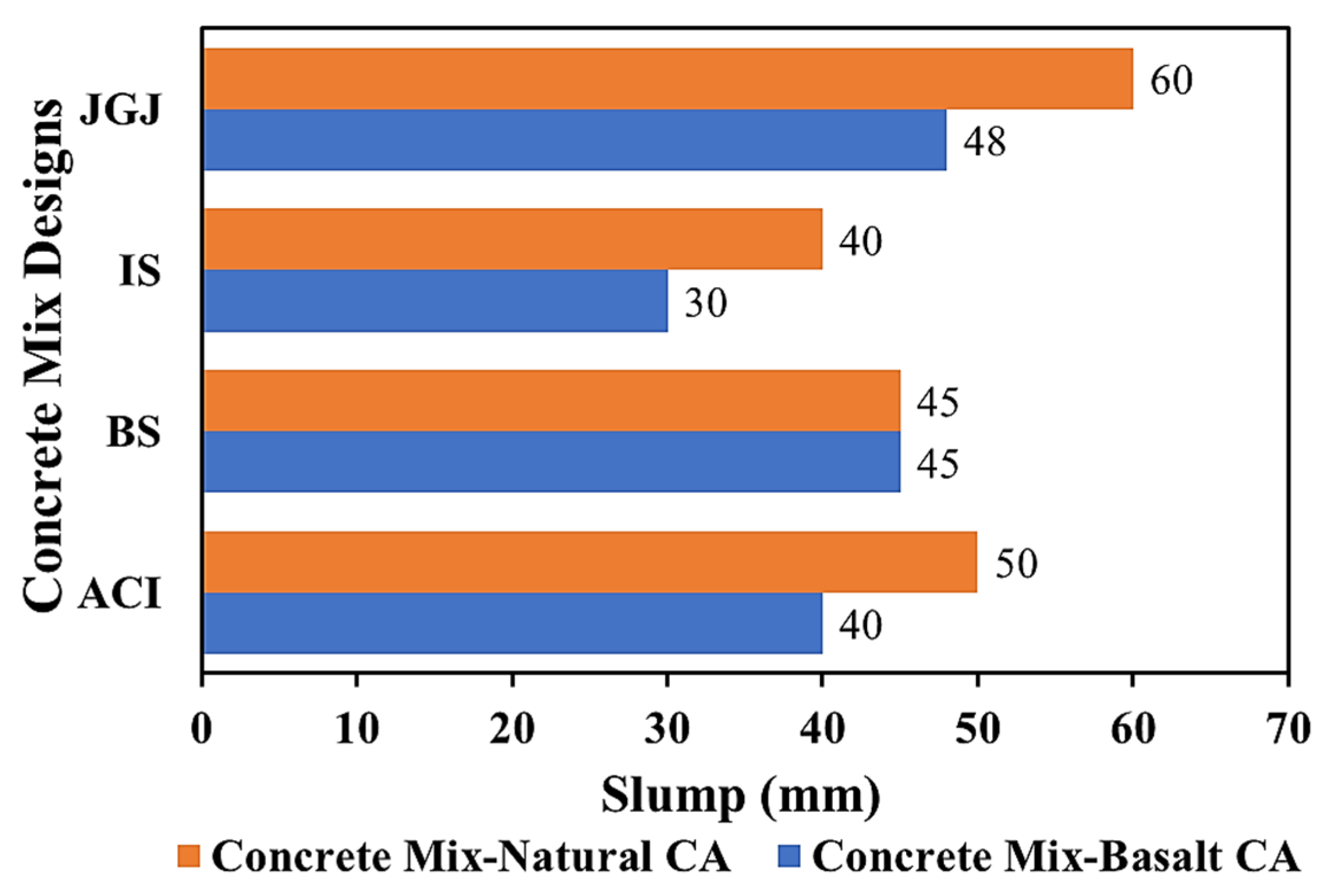
Slump tests were conducted to determine the functionality of fresh concrete. The slump results are shown in Figure 6. The ACI, BS, IS, and JGJ mixtures made of basalt CA provided slump results within the ranges specified by the CMD codes, i.e., 40 mm, 45 mm, 30 mm, and 48 mm, respectively. The ACI, BS, and IS mix designs using natural CA achieved the targeted slump results as per the respective mix design codes, i.e., 50 mm, 45 mm, and 40 mm. The JGJ concrete mixture had a maximum slump value of 60 mm, which was slightly higher than the specified range. The JGJ concrete mixture achieved higher slump value due to the higher water content, whereas the IS mixture had the lowest slump value due to the lower water content. In both cases, when basalt CA and natural CA were utilized, the BS concrete offered the same slump, i.e., 45 mm. The ACI, IS, and JGJ mixtures with natural CA offered 20%, 25%, and 20% higher slump values than those with basalt CA. According to the comparison, it is clear that the CA type, shape, and water content in the mixture play a crucial role in determining the workability of fresh concrete. Moreover, the lower workability of fresh concrete mixtures containing crushed basalt CA resulted in higher CS of hardened concrete.

4.2. Failure Mode

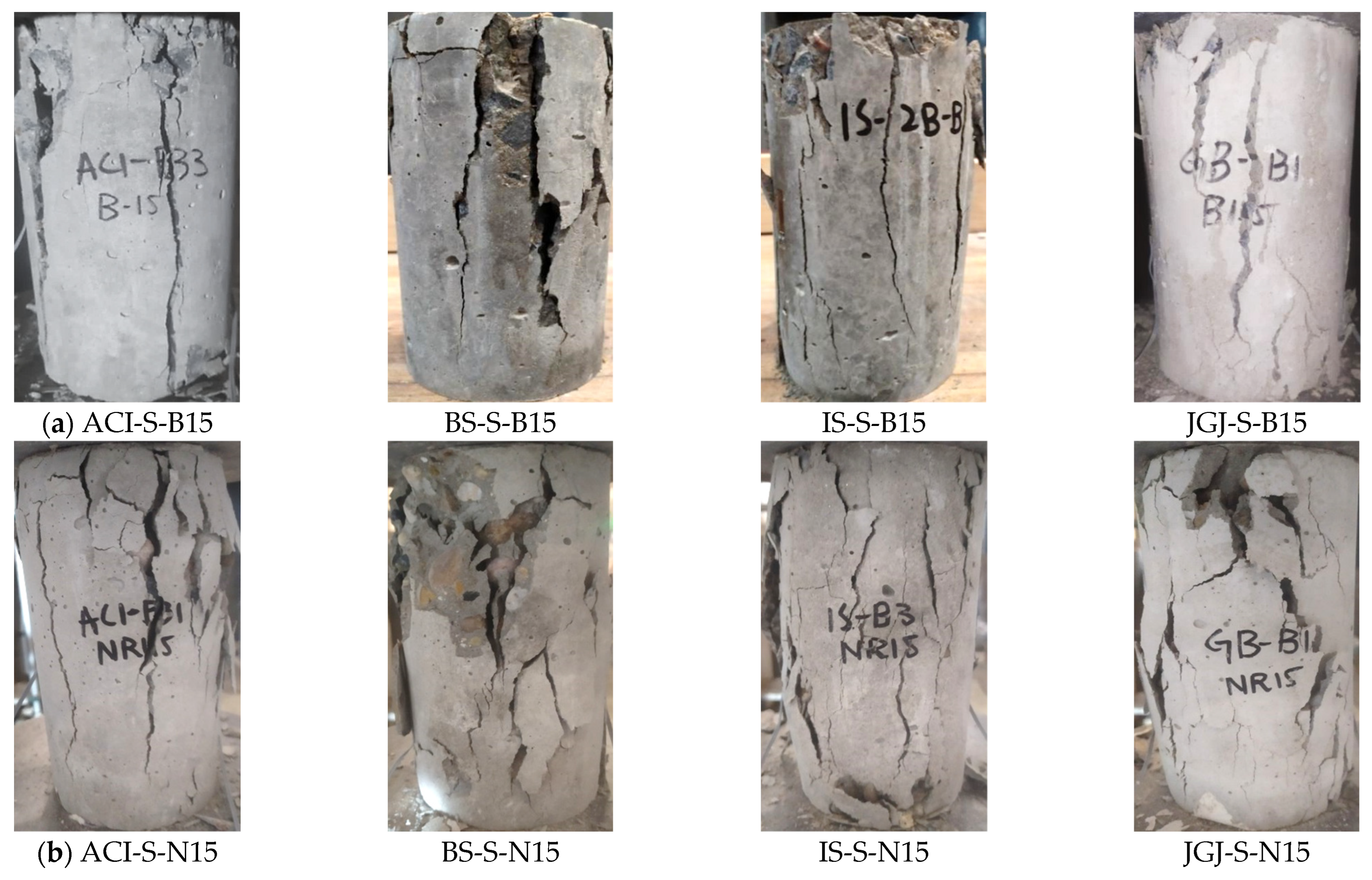
During axial compressive loading, the initial cracks developed at the top region of the specimens and propagated downwards. As the peak load (P_max) was reached, the loading rate decreased gradually, and an uneven crack structure was established with diagonal and vertical columnar macro cracks. With attentive observation during testing, the first crack in the cylindrical specimens made with basalt CA and natural CA appeared at approximately 65% and 50% of their respective P_max. 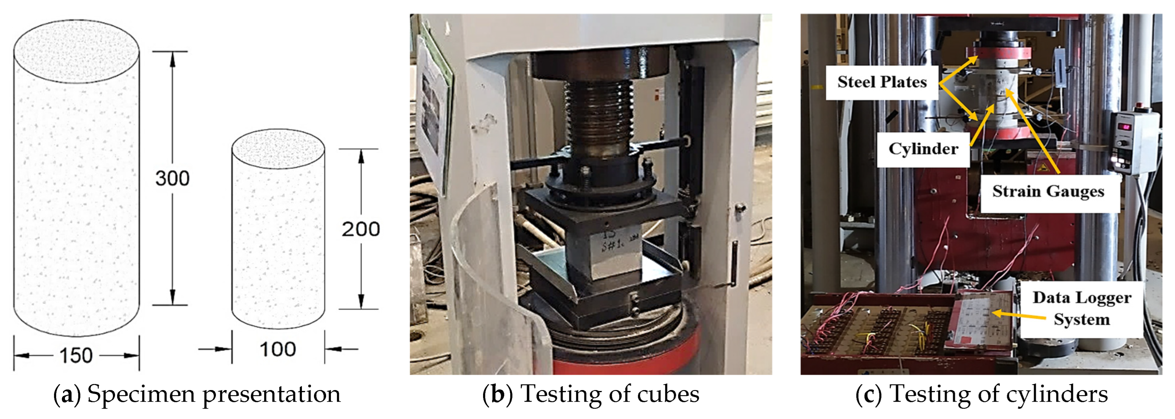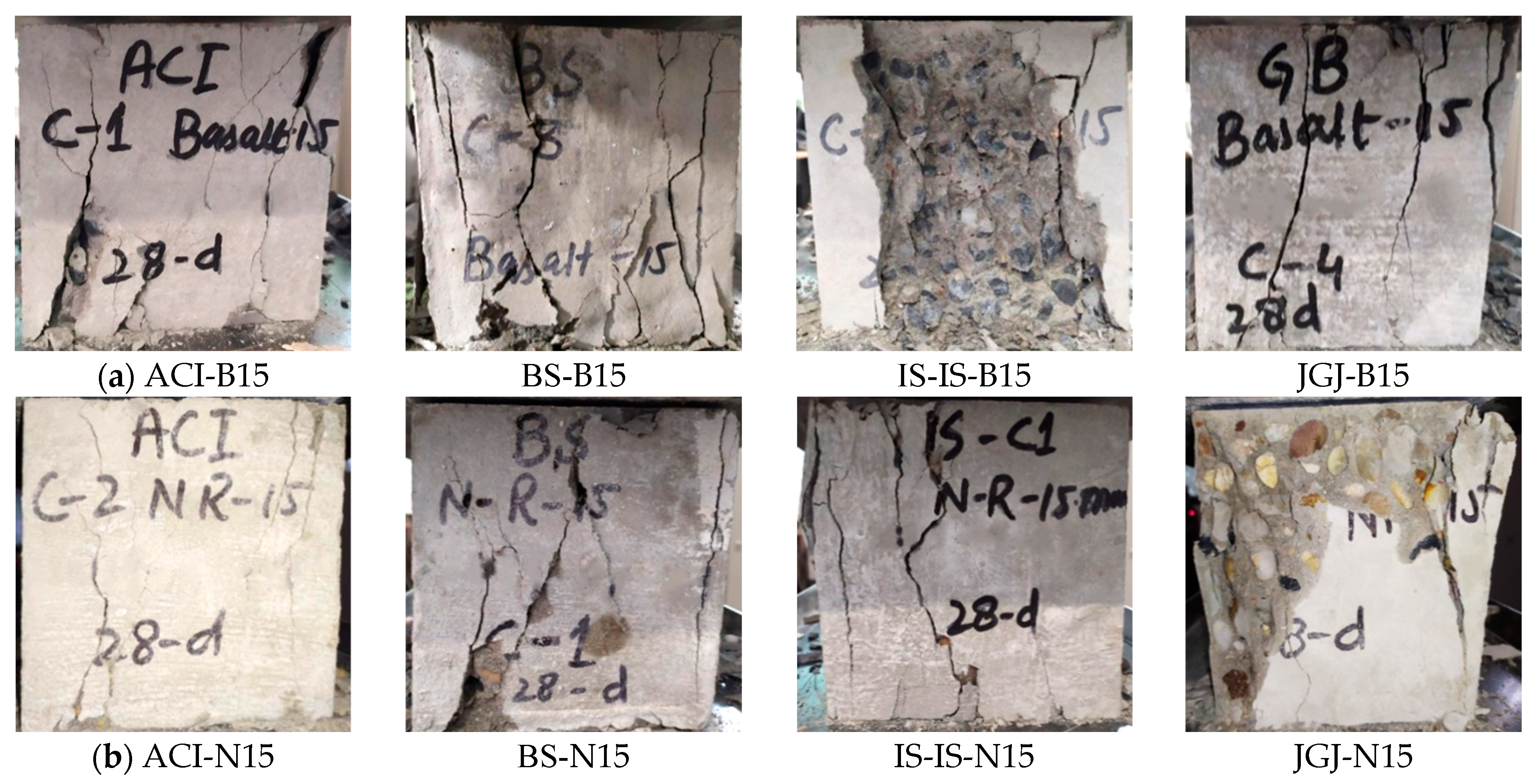The crack aspect ratios at P_max for large cylinders and small cylinders of basalt CA were 0.75 and 0.85, respectively, whereas the aspect ratios of cracks at P_max for large and small cylinders made with natural CA were 0.82 and 0.85, respectively. Longitudinal splitting in columnar pattern failure was observed along the direction of load application in the cylindrical specimens. 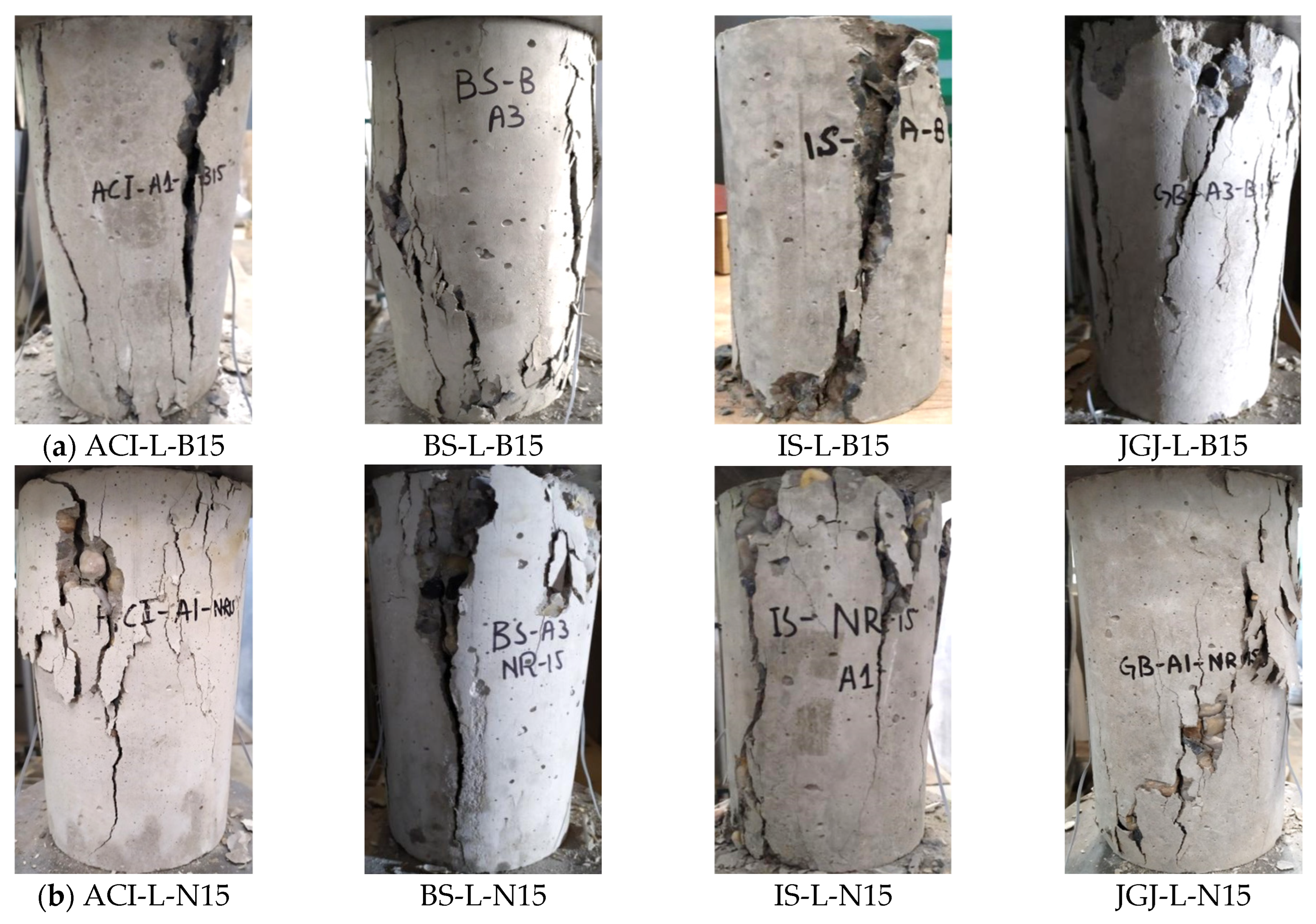For the cube specimens, failure occurred in a vertical pattern, diagonal shear occurred from top to bottom, and the matrix also flaked from the sides, as shown in Figure 7a,b. The failure modes of the cylindrical specimens are illustrated in Figure 8 and Figure 9. 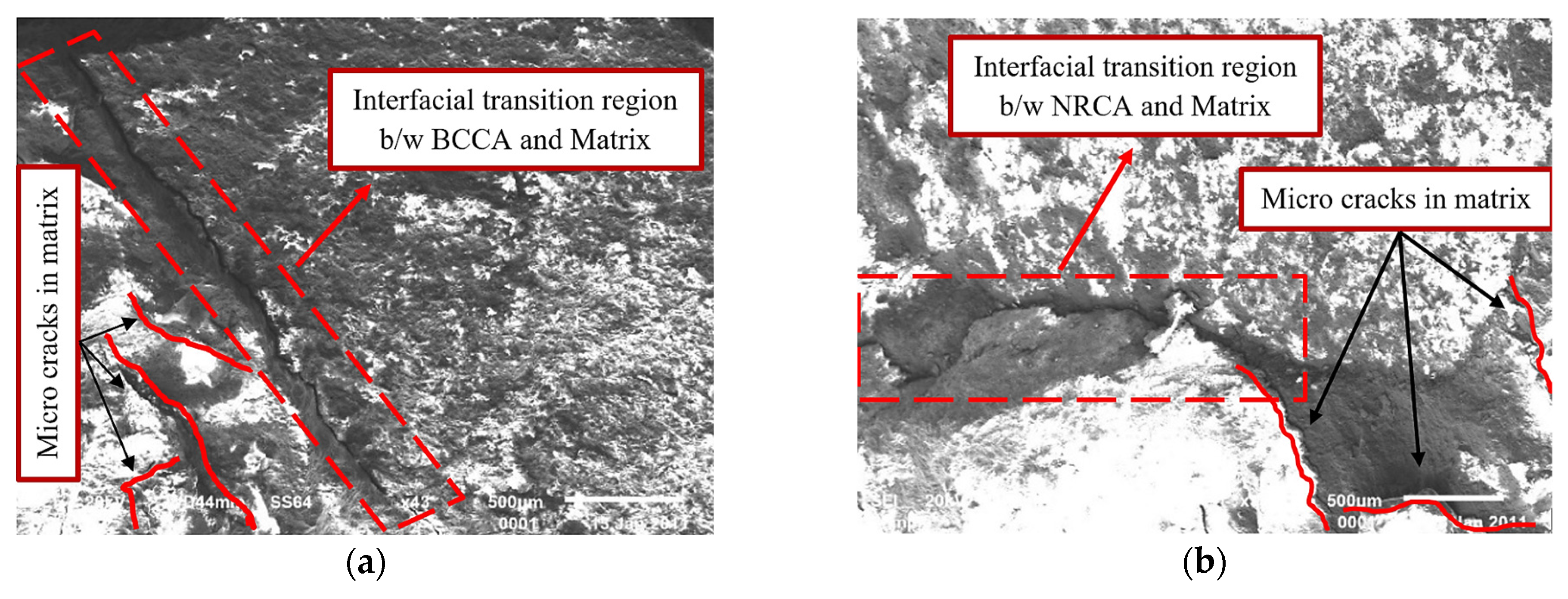The failure patterns of the cylindrical specimens are interpreted and compared with the listed failure patterns in ASTM C39 [77]. Cylinders with basalt CA mainly displayed Type 3 failure pattern (columnar/shear), which indicates robust interlock of aggregates and increased friction along the cracks. Type 1 and Type 2 (cone and split) failure patterns were more common in cylinders with natural CA, particularly in the smaller cylinders. These failures are associated with reduced interlock and smoother aggregate surface. Due to less end constraint and better stress distribution, large cylinders often displayed more symmetric and consistent failure modes (Type 3 failure modes). All the detected failure modes fit within permitted patterns, demonstrating appropriate testing arrangement and acceptable failure reactions. After the test, the inner cross-sections were examined. Debonding between CA and matrix occurred mainly in the specimens prepared with natural CA, and crushing of the aggregates was also detected. Less debonding was observed in the case of basalt CA specimens, but in some cases, the CA were also crushed. Scanning electron microscopic (SEM) examination was performed to evaluate the microstructural behavior of the tested specimens, as shown in Figure 10. The interfacial transition zone (ITZ) was identified as the main area of vulnerability. It was characterized by a noticeable detachment between the aggregates and the cement matrix. This area, distinguished by porosity and micro-voids, enables the initiation and spread of cracks. The observed cracking patterns indicate that fractures spread along the weakest channels, such as the ITZ and pre-existing microcracks. This ultimately results in aggregate fracture and matrix collapse. In addition to SEM analysis, the qualitative visual examination of the fractured surfaces revealed that matrix cracking and ITZ debonding were the primary causes of failure, with aggregate fracture occurring in approximately 12% to 18% of the failure surface, indicating that matrix-controlled failure predominated. Specimens with basalt CA provided stronger interface bonds due to their angular shape and rough surface texture compared to natural CA.

4.3. Compressive Strength

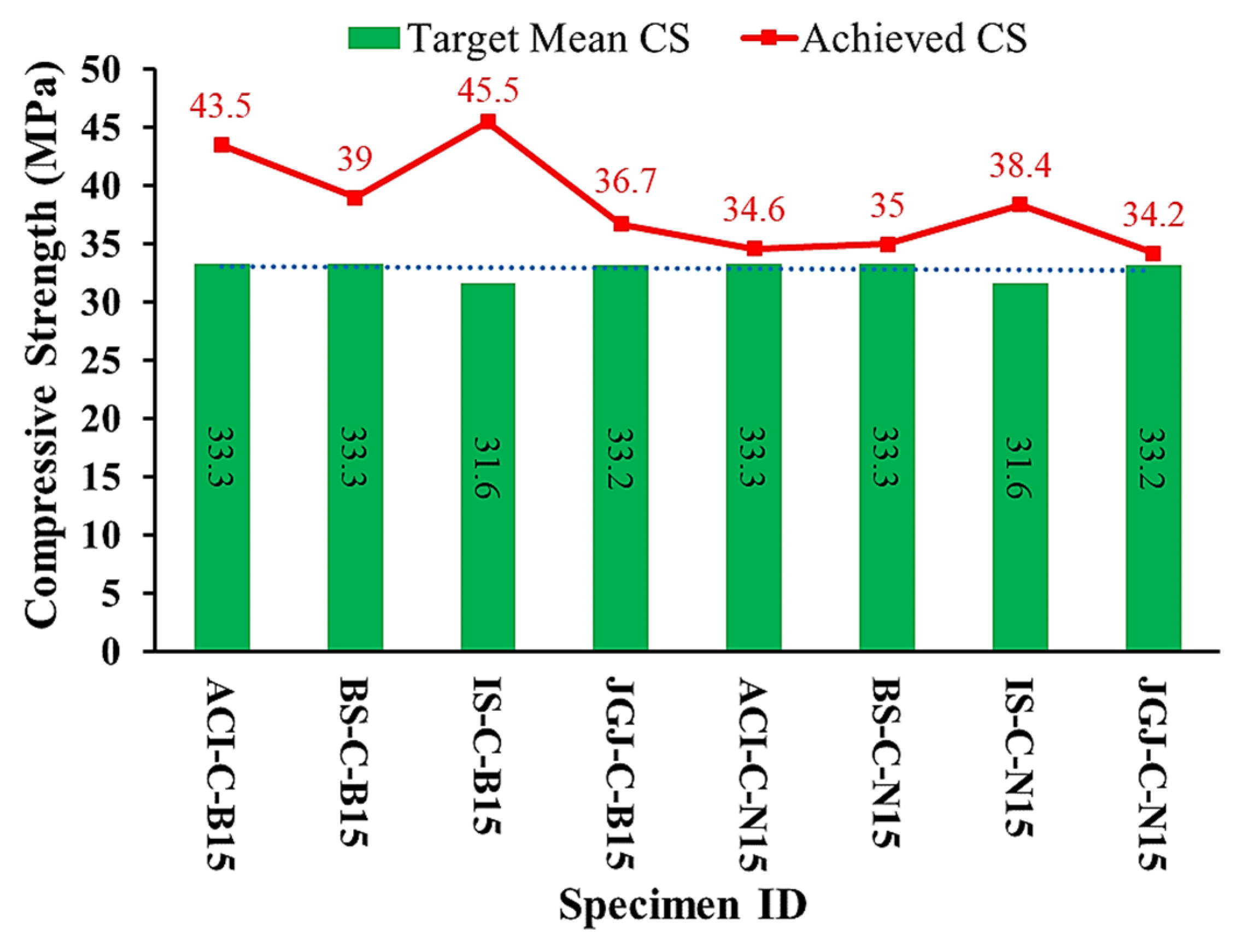
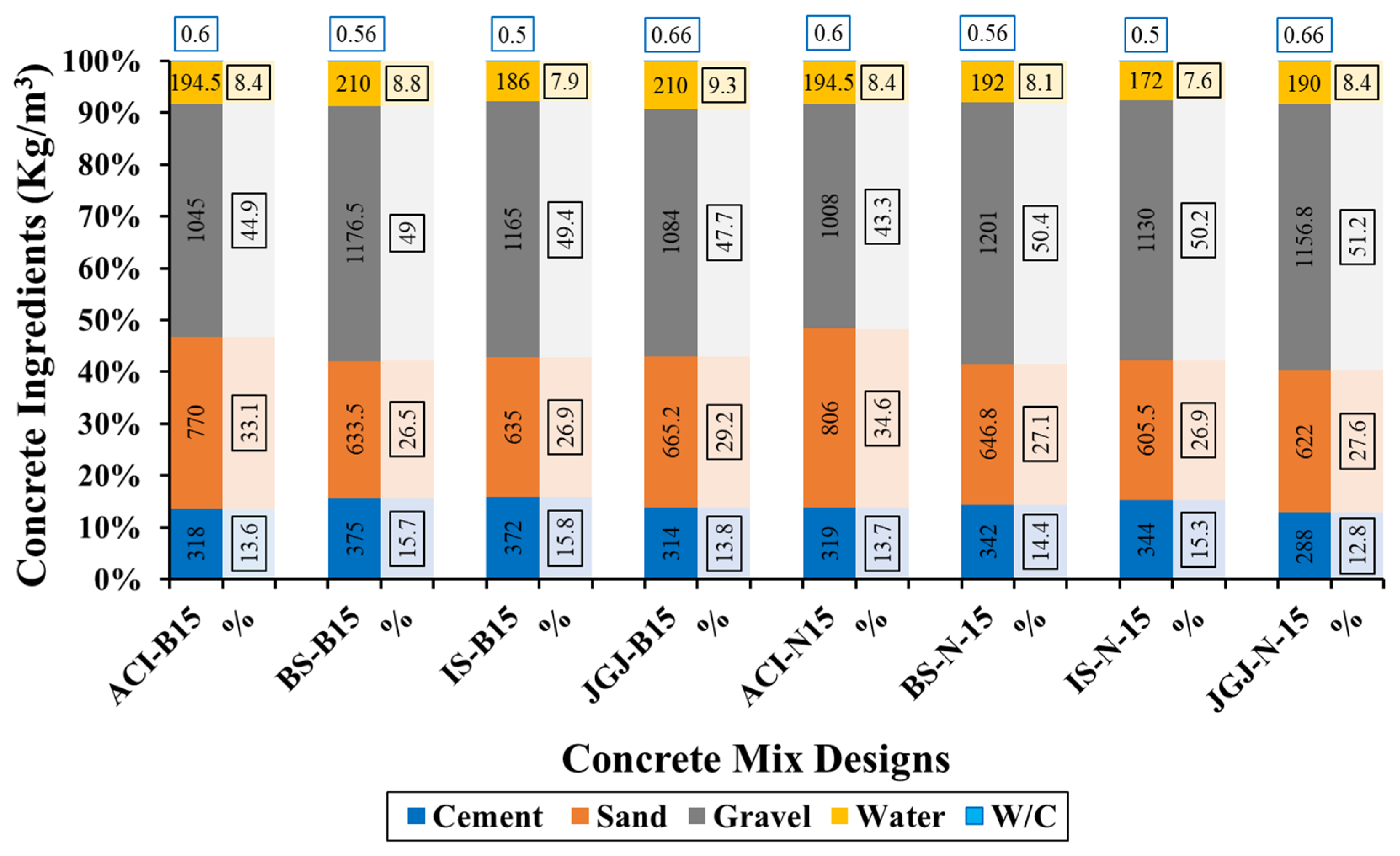
The target mean CS was calculated using Equations (14), (15), (16), and (17) specified by the ACI, BS, IS, and JGJ codes, respectively. Figure 11 presents the CS of cubes made with basalt and natural CA. The first letter of the specimen ID indicates the CMD code, the second letter indicates a cube, and the third letter represents the CA type of size 15 mm. Using basalt CA, the cubes of each CMD code surpassed the targeted mean CS. The ACI-C-B15, BS-C-B15, IS-C-B15, and JGJ-C-B15 specimens achieved 23.4%, 14.6%, 30.5%, and 8% higher CS than the designed CS, confirming the accuracy of the CMD calculations. In the case of natural CA concrete, the ACI-C-N15, BS-C-N15, IS-C-N15, and JGJ-C-N15 cubes exhibited 3.8%, 4.9%, 17.7%, and 3% higher CS than the designed CS, respectively, indicating the precision of the concrete mix proportion. The CS of cubes made with basalt CA was significantly higher than their counterparts made with natural CA. The ACI-C-B15, BS-C-B15, IS-C-B15, and JGJ-C-B15 presented 20.5%, 10.3%, 15.6%, and 7% higher CS than the cubes produced with natural CA of the same CMD codes, respectively. The explanation for the higher CS attained by the cubes of basalt CA is its shape, surface texture, and higher crushing strength, owing to a stronger interface bond developed between the matrix and basalt CA, resulting in a noticeably higher CS. The second cause is the W/C ratio, which is more influential in the case of concrete with natural CA.

$${f^{\prime }}_{cr}={f^{\prime }}_c+s$$

(14)

$$f_m=f_{ck}+k\sigma$$

(15)

$${f^{\prime }}_{ck}=f_{ck}+1.65\times s$$

(16)

$$f_{cu,0}\ge f_{cu,k}+1.645\sigma$$

(17)

where ${f^{\prime }}_{cr}$, $f_m$, ${f^{\prime }}_{ck}$, and $f_{cu,k}$ indicate the target mean strength, ${f^{\prime }}_c$, $f_{ck}$, and $f_{cu,k}$ indicate the characteristic CS (MPa) of the concrete at 28 days, $s$ and  $\sigma$ indicate the standard deviation, and $k$ is the risk factor.

The experimental results for large and small cylinders incorporated with basalt and natural CA are presented in

Table 2. Experimental results of large cylinders 150 × 300 (mm) and small cylinders 100 × 200 (mm).

Specimen ID	CA Type and Size	CS (MPa)	Ec (GPa)	SD (MPa)	CV (%)	Accumulated Energy (kN·mm2)	Fracture Energy (kN·mm)
ACI-L-B15	Basalt (15 mm)	34.4	27,760	2.1	6.0	984.0	304.5
BS-L-B15		30.2	25,972	2.2	7.3	1114.0	428.5
IS-L-B15		36.3	28,444	2.7	7.3	1021.0	300.0
JGJ-L-B15		30.7	26,319	3.0	9.3	886.0	295.5
ACI-L-N15	Natural (15 mm)	24.1	23,176	1.7	6.8	606.0	222.8
BS-L-N15		22.5	22,365	2.6	11.7	596.0	241.2
IS-L-N15		22.2	22,201	2.2	9.7	677.0	270.5
JGJ-L-N15		19.3	20,762	1.4	7.0	469.0	212.5
ACI-S-B15	Basalt (15 mm)	32.0	26,712	2.4	7.5	384.6	83.5
BS-S-B15		24.5	23,328	1.7	6.7	294.0	140.7
IS-S-B15		33.0	27,132	1.5	4.5	318.4	140.5
JGJ-S-B15		28.2	25,076	1.6	5.7	283.5	123.5
ACI-S-N15	Natural (15 mm)	21.3	21,751	3.2	14.5	165.5	83.5
BS-S-N15		20.5	21,366	2.1	10.3	164.6	73.0
IS-S-N15		19.8	20,985	0.9	4.5	165.5	78.0
JGJ-S-N15		19.6	20,870	2.0	10.0	178.5	87.4

. Each result presents an average of three measurements. The variability in the CS results is indicated by the standard deviation (SD) and coefficient of variation (CV), calculated using Equations (18) and (19). Lower SD values suggest better consistency in the CS results. Similarly, lower CV values indicate less relative variability in the CS results compared to the mean result. In the ID of the specimens, the first letter indicates the CMD code, the second letter, L or S, shows the size of the cylinder, and the third letter, B15 or N15, indicate the CA type and size. The cylinders of the basalt CA offered notably higher CS than the cylinders of the natural CA in each of the four CMD codes. In the category of large cylinders, ACI-L-B15, BS-L-B15, IS-L-B15, and JGJ-L-B15 offered 30%, 25.5%, 39%, and 37% higher CS than their counterparts. In the case of small cylinders, ACI-S-B15, BS-S-B15, IS-S-B15, and JGJ-S-B15 achieved 33.4%, 16.3%, 40%, and 37% higher CS, respectively, than the small cylinders of the natural CA. The CS varies with the cylindrical dimensions as the large cylinders exhibited higher CS than the smaller cylinders. The large cylinders, i.e., ACI-L-B15, BS-L-B15, IS-L-B15, and JGJ-L-B15, offered 7%, 19%, 9%, and 8% higher CS, respectively, than the small cylinders. The same tendency was found for the large cylinders prepared with natural CA, i.e., ACI-L-N15, BS-L-N15, and IS-L-N15 achieved 11.6%, 9%, 10.8%, and 10% higher CS than the smaller ones. The large cylinders JGJ-L-N15 attained the same CS as the small cylinders JGJ-B-N15. The specimen size-related trend in the present study, i.e., larger cylinders attained higher CS than smaller cylinders is consistent with several earlier findings in the literature [94,95,96,97]. Concrete with basalt CA offered significantly higher CS than natural CA concrete due to its higher crushing strength, shape, and surface texture. All these properties are involved in providing a strong connection between the cement matrix and CA, which results in superior compression characteristics. The results also revealed the cylindrical specimen size effect on the CS of NSC.

$$SD=\sqrt{{\displaystyle \frac{1}{n-1}}}{{\displaystyle \sum }}_{i=1}^n{(x_i-x^{\prime } )}^2$$

(18)

$$CV={\displaystyle \frac{S.D}{x^{\prime }}}\times 100$$

(19)

where SD is the sample standard deviation, n indicates the number of CS results, xi indicates the individual CS result, and x′ is the mean CS result of all the samples.

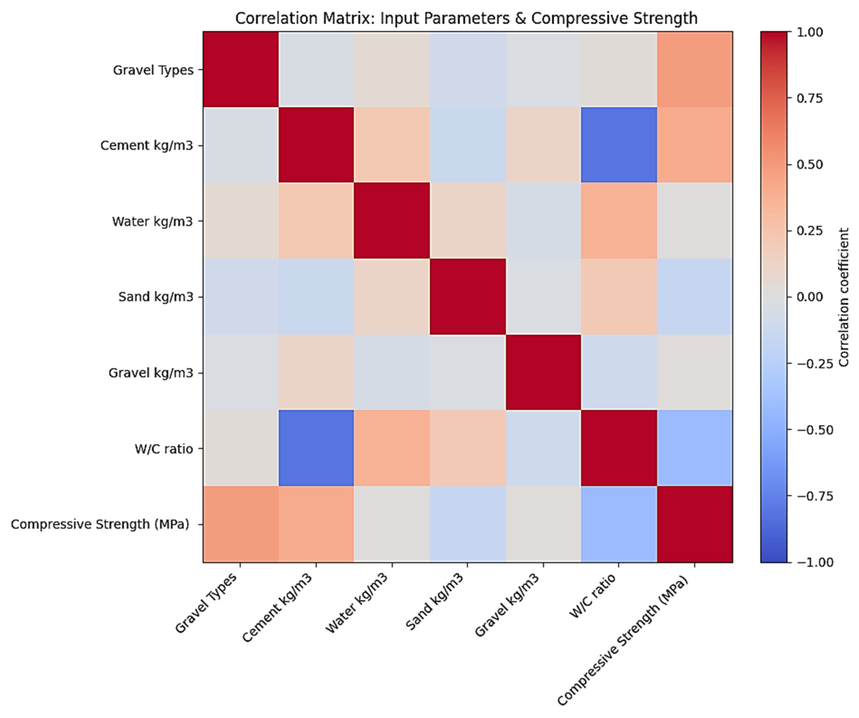
A correlation matrix, as illustrated in Figure 12, is produced to better understand how concrete mixture proportioning factors affect CS. The ingredients’ positive correlations are indicated in red, whereas negative correlations are shown in blue, and the color intensity represents correlation magnitude. The matrix depicts the linear connections between important factors of mix design and CS. The CA type has the strongest positive association with CS, underscoring that concrete CS capacity is greatly influenced by CA source, type, and shape. Furthermore, a relatively strong positive connection is discovered between cement content and CS, showing that larger cement fractions lead to increased CS. On the other hand, W/C ratio showed a moderate negative relationship with CS, confirming the classical concrete behavior. Increased porosity and poor past quality are common outcomes of higher W/C ratios, which results in reduced CS. The water content displayed a slightly negative effect on CS. A higher water quantity in the mix can dilute the cement paste, although the W/C ratio is more important in strength performance than water alone. The aggregate content (sand and gravel) reveals insignificant relationships, suggesting that within the investigated limits, their impact on CS is minor. This investigation confirms that CA type and cement–paste ratio have a major impact on concrete CS, with water content and aggregate amount having minor impacts. This correlation structure validates the findings of the experimental program.

4.4. Load–Displacement Behavior

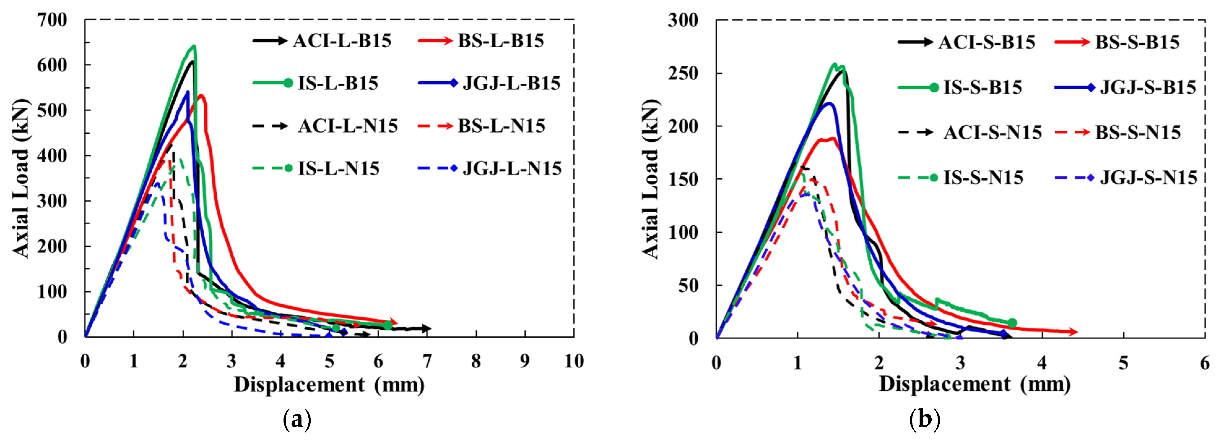
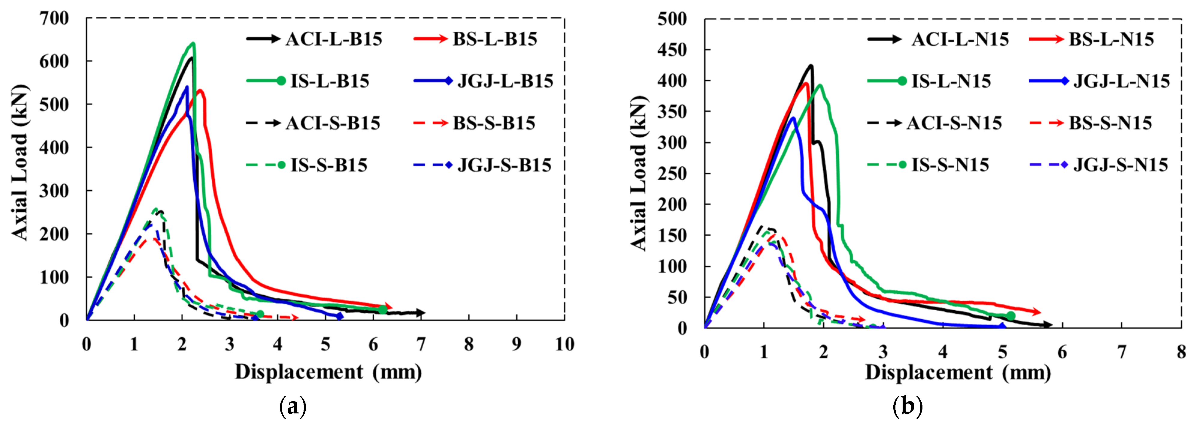
In terms of load–displacement curves, the compressive behaviors of the cylindrical specimens are evaluated. Figure 13a,b and Figure 14a,b illustrate the load–displacement performance of large and small cylinders made with basalt CA and natural CA. From the curves, it is evident that the CA type had no impact on the elastic region, as the curves showed nearly identical linear behavior. However, there is a noticeable effect of CA type in the transition region of the load–displacement curves up to the P_max of both large and smaller cylinders. After reaching their respective P_max, the basalt CA large and small cylinder curves, i.e., ACI-L-B15, BS-L-B15, IS-L-B15, and JGJ-L-B15 and ACI-S-B15, BS-S-B15, IS-S-B15, and JGJ-S-B15, descended in a ductile manner and showed more resistance against the applied load at the end compared to the cylinders made with natural CA. In the case of cylinders made with natural CA, the load–displacement curves exhibited brittle failure. The load–displacement curves indicate a notable impact of CA type and shape on the post-peak behavior of the concrete cylinders. These variations in the transition and post-peak phases are not only due to the CA type and shape but can also be associated with the CMD code effect. It is noted that the post-peak softening slope could not be reliably calculated for most specimens, as the load–displacement curves exhibited abrupt or near-vertical drops after the peak load, indicating brittle failure with minimal softening behavior. This was particularly evident in specimens prepared with natural coarse aggregates, where the post-peak phase was characterized by rapid load reduction and limited ductility.

Table 2 presents the determined static elastic modulus (E_c) for all cylindrical specimens. Concrete incorporating basalt CA exhibited consistently higher E_c than that with natural CA, ranging from 8% to 23% higher, depending on the mix design code and specimen size. This enhancement is attributed to the angular particle shape, rough surface texture, and higher inherent stiffness of basalt, which promote a stronger interfacial transition zone (ITZ) and more effective stress transfer between matrix and aggregate. The trend holds for both large (150 × 300 mm) and small (100 × 200 mm) cylinders, demonstrating that the aggregate type governs composite rigidity more than geometric scaling.

4.5. Energy Accumulation

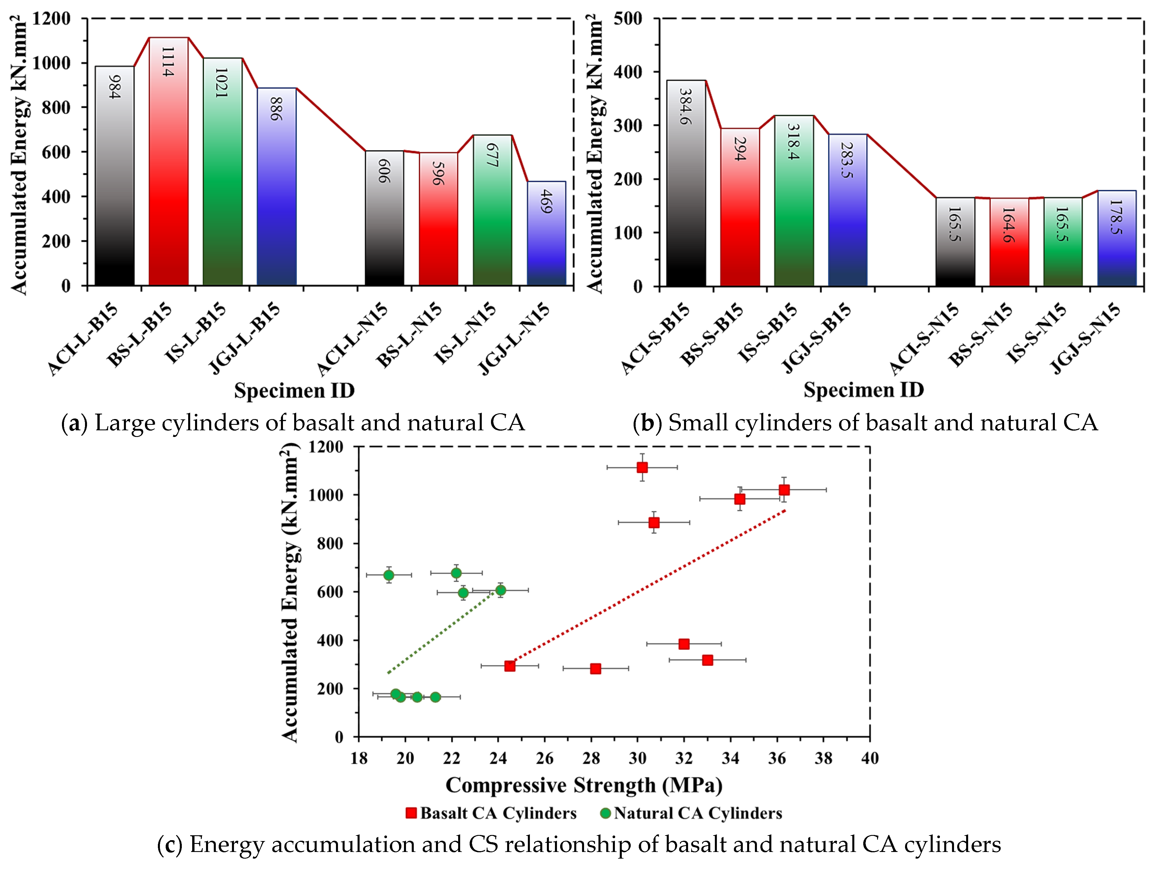
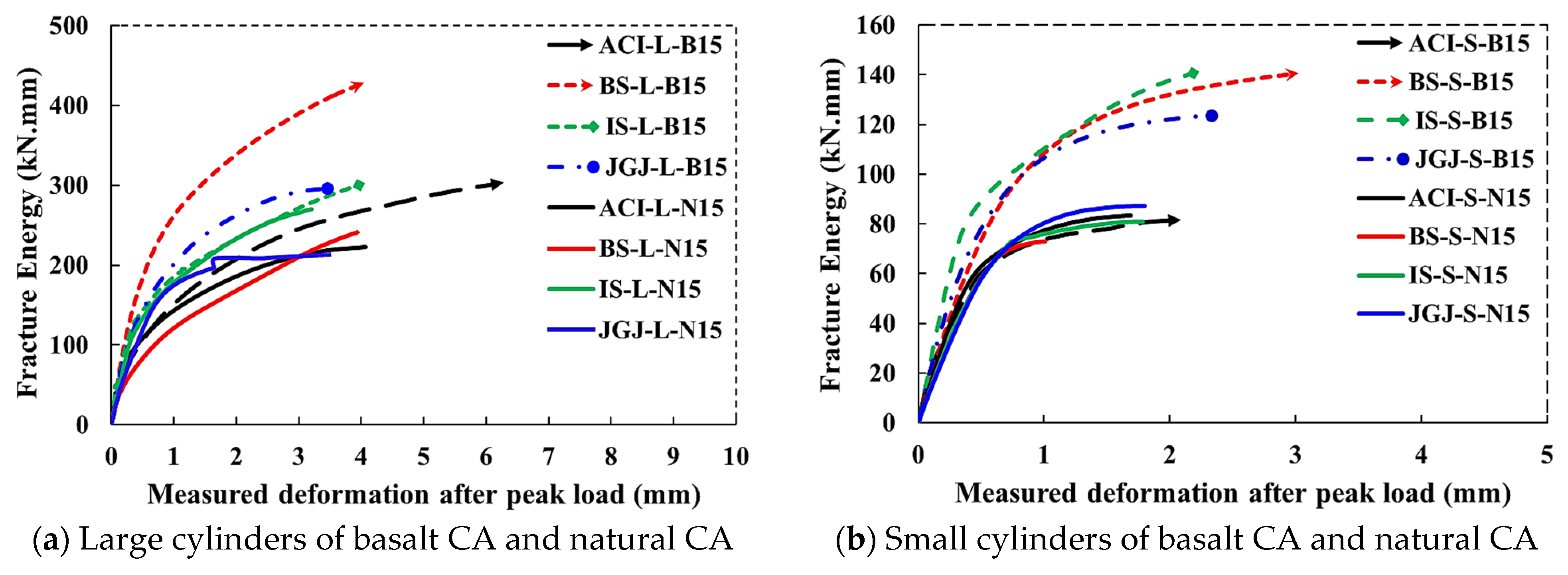
The whole cumulative area beneath the load–displacement curve was calculated as the accumulated energy (G_A). The results of the G_A of cylinders made with basalt CA and natural CA are given in Table 2 and Figure 15a,b. The results clearly show that the cylinders prepared with basalt CA exhibited significantly higher G_A than their counterparts made with natural CA. In the category of large cylinders, ACI-L-B15, BS-L-B15, IS-L-B15, and JGJ-L-B15 offered 38.4%, 46.6%, 33.7%, and 47% higher G_A than ACI-L-N15, BS-L-N15, IS-L-N15, and JGJ-L-N15, respectively. Similarly, the smaller cylinders of basalt CA, i.e., ACI-S-B15, BS-S-B15, IS-S-B15, and JGJ-S-B15, achieved 57%, 44%, 48%, and 37% higher G_A than their counterparts made with natural CA. The results confirmed the significant impact of CA type and shape on the energy dissipation of circular cross-sections. Furthermore, the scatter plot in Figure 15c clearly shows a positive correlation between G_A and CS, with basalt CA cylinders showing significantly greater G_A than natural CA cylinders, indicating greater resistance against axial compressive load. The strength–energy relationship trend indicates that the improved G_A capacity is positively correlated with higher CS.

4.6. Post-Peak Fracture Energy

The post-peak fracture energy (G_F) is computed from the peak load point to the lowest point of the load as the region under the load–displacement curve. It concerns concrete’s ability to resist applied compressive load after exceeding the P_max. Table 2 presents the G_F results for large and small cylinders made with basalt CA and natural CA. The results indicated that the specimens fabricated with basalt CA exhibited significantly higher G_F than the specimens prepared with natural CA. In the category of large cylinders, ACI-L-B15, BS-L-B15, IS-L-B15, and JGJ-L-B15 offered 26.8%, 43.7%, 9.8%, and 28% higher G_F than ACI-L-N15, BS-L-N15, IS-L-N15, and JGJ-L-N15, respectively. In the case of small cylinders, the specimens prepared with basalt CA had an improved G_F compared to those made with natural CA. Due to catastrophic failure at the maximum load, small cylinders had lower G_F. The specimens ACI-S-B15 and ACI-S-N15 achieved the same G_F, whereas BS-S-B15, IS-S-B15, and JGJ-S-B15 attained 48%, 44.5%, and 29.2% improved G_F compared with BS-S-N15, IS-S-N15, and JGJ-S-N15, respectively. The resultant G_F curves of large and small cylinders are illustrated in Figure 16a,b.

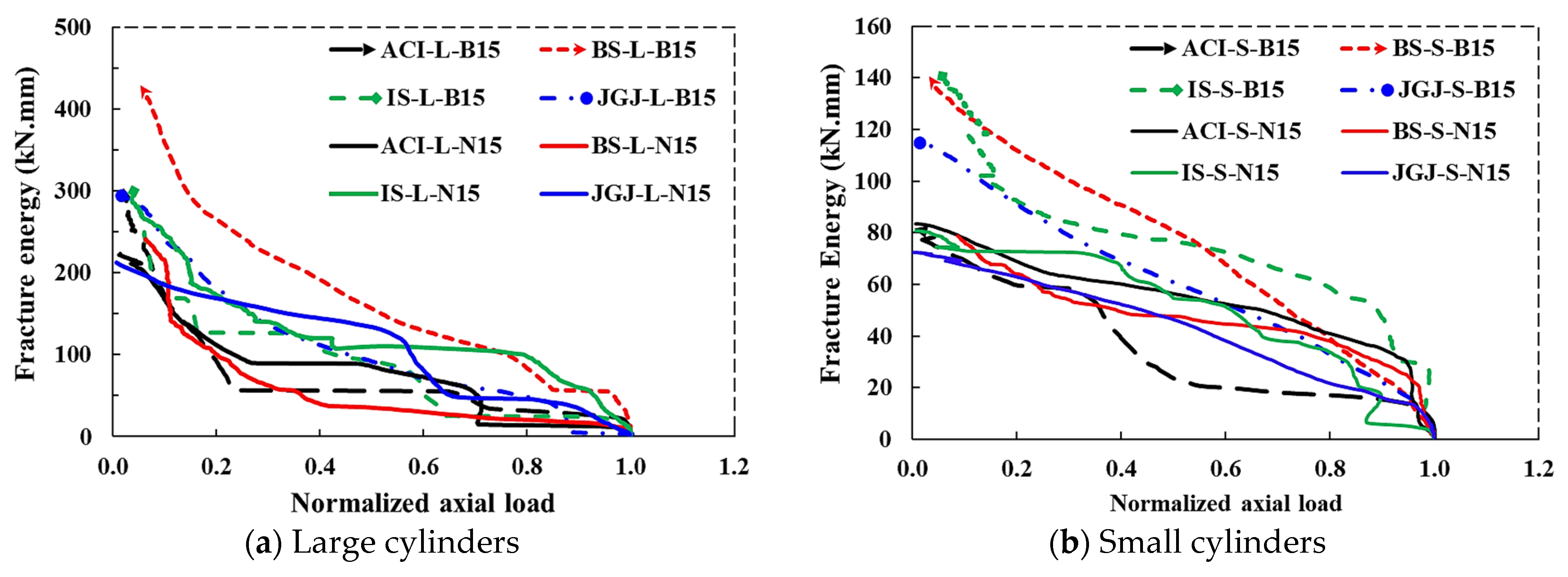
The post-peak phase in the load–displacement curve of concrete is critical for comprehending G_F and ductility. The post-peak behavior of large and small cylinders containing basalt CA and natural CA is depicted in Figure 17a,b by plotting G_F against the normalized axial compressive load. Compared with natural CA concrete, basalt CA concrete exhibits a less steep decline in normalized axial load. This shows enhanced post-peak performance, indicating that basalt CA concrete retains the load-bearing capability better after P_max. This is indicative of less ductile concrete, as natural CA results in less interlocking and binding strength with the cement matrix. It also shows more brittle failure with a rapid drop in the post-peak load-bearing capacity. Basalt CA greatly increases the post-peak load-bearing ability and energy absorption capacity of concrete due to its high crushing strength, angularity, and rough surface texture, leading to enhanced bonding properties. Regardless of the CMD codes being utilized, basalt CA is a better option than natural CA for applications that require increased strength, ductility, and toughness.

4.7. Performance Evaluation of ML Algorithms Based on Statistical Analysis

To forecast the CS of concrete, four ML models, i.e., XGB, GBR, RF, and SVR were developed using the Python Scikit-learn package (Python 3.11.3), (Scikit-learn 1.2.2). To guarantee consistent scaling, the Standard Scaler module from Scikit-learn was first used to standardize the dataset’s features. This section presents a statistical-based comparison of these four ML models that predicted the CS of concrete. A series of statistical parameters such as R², MAE, MAPE%, MSE, and RMSE were employed to quantitatively assess the performance of these ML models, as shown in

Table 3. Statistical parameters of the MLs’ models performance.

ML Models	R2	MAE	MAPE%	MSE	RMSE
XGB	0.92	0.59	2.3	1.07	1.04
GBR	0.92	0.56	2.16	1.14	1.07
RF	0.93	0.59	2.27	0.94	0.97
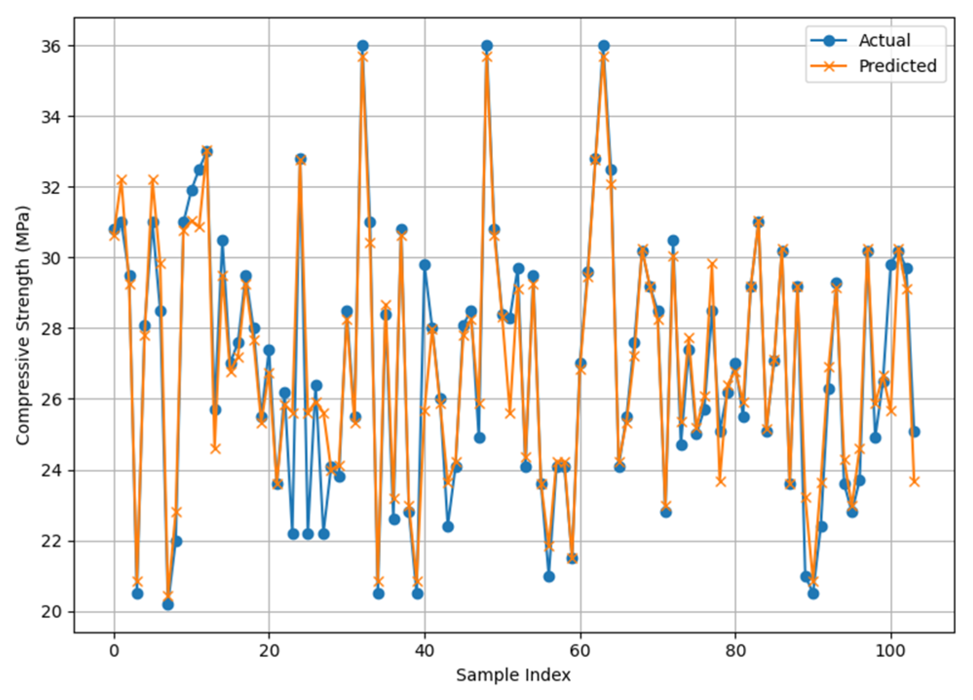
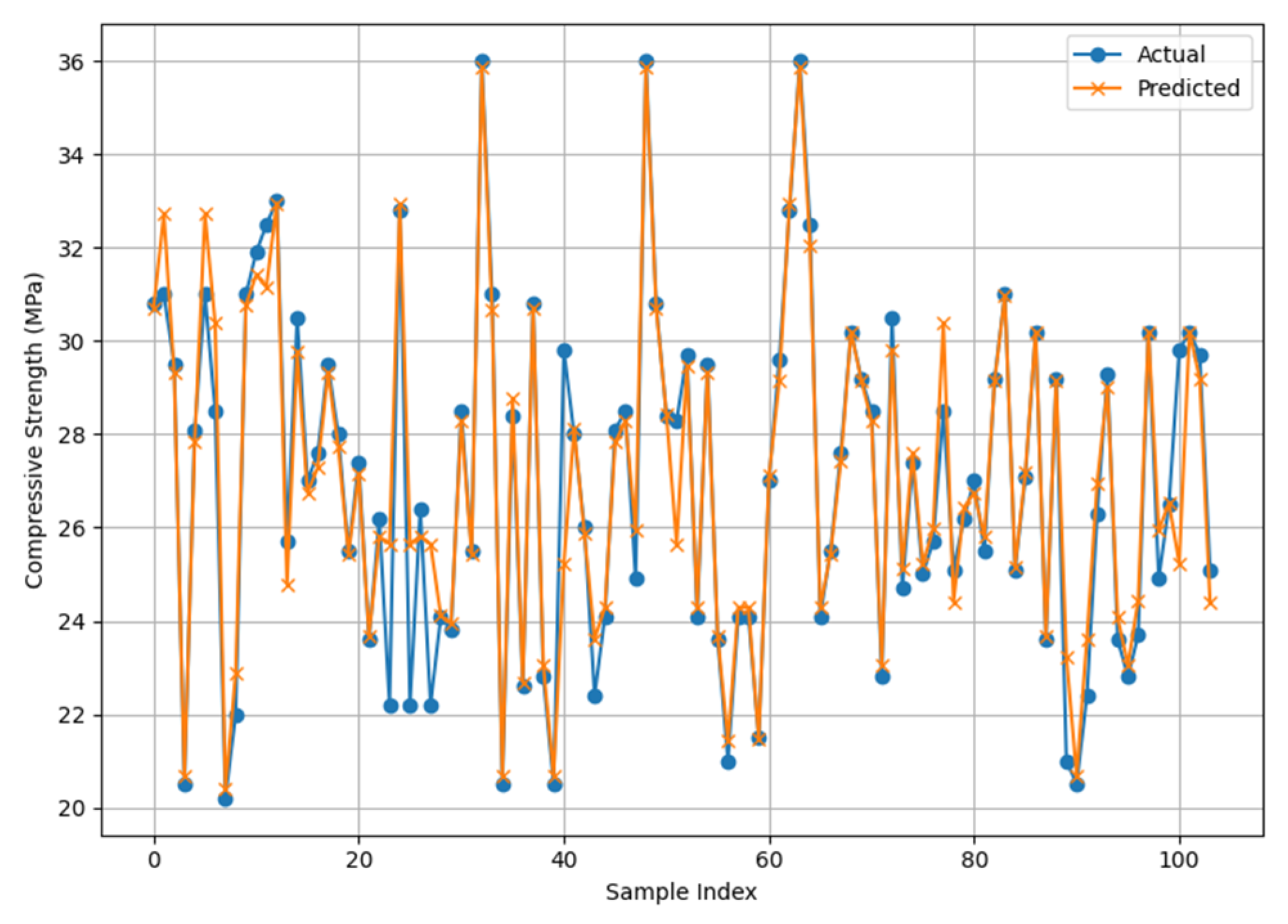
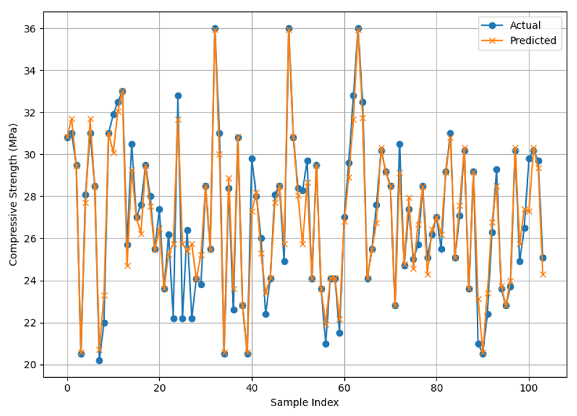
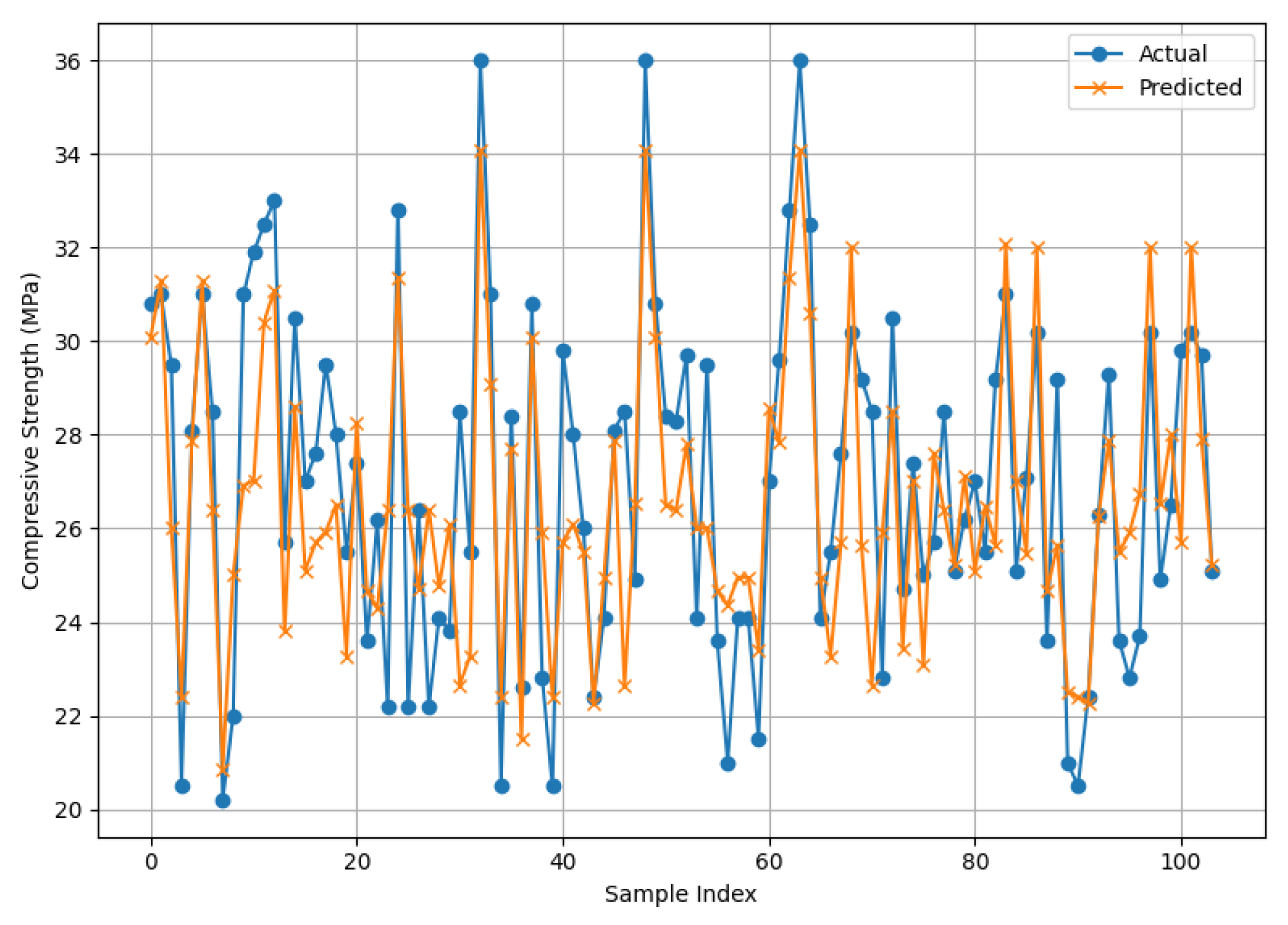
SVR	0.60	1.95	7.33	5.39	2.32

. The graphical comparison of experimental and predicted CS results from the ML models is illustrated in Figure 18, Figure 19, Figure 20 and Figure 21. The prediction accuracy and generalization potential of each model for calculating the CS of concrete were thoroughly evaluated using these criteria. The statistical analysis demonstrated that the ensemble-based models, i.e., RF, XGB, and GBR consistently showed excellent prediction ability. The models XGB and GBR both obtained R² of 0.92, showing that the models account for more than 92% of the variation in the experimental CS data. RF marginally surpassed the XGB and GBR, with the highest R² of 0.93, signifying enhanced fit and generalization capability. Conversely, SVR demonstrated low performance (R² = 0.60), which implies that it has inadequate ability to capture the dataset’s nonlinear connections.

Additional analysis of the error metrics further validates these findings. In terms of average prediction error compared to the actual CS values, GBR exhibited the lowest MAE (0.56) and MAPE (2.16%), indicating marginally higher precision. XGB and RF demonstrated excellent accuracy and resilience, with MAE values of 0.59 and MAPE values of 2.3% and 2.27%, respectively. Furthermore, RF attained the lowest MSE of 0.94 and RMSE of 0.97, underscoring its exceptional capacity to reduce significant discrepancies between predicted and actual CS values. Conversely, SVR demonstrated much larger errors, i.e., MAE = 1.95, MAPE = 7.33%, MSE = 5.39, and RMSE = 2.32, showing its poor predictive potential for this dataset.

The comparison reveals that RF achieved superior performance, effectively balancing a high variance explanation (R² =0.93) with the lowest MSE and RMSE metrics. This positions RF as the most dependable model for predicting the CS of concrete among the four assessed models. Additionally, XGB and GBR exhibited impressive predictive accuracy, positioning them as viable alternatives, especially in situations where boosting methods are preferred. Although SVR is well-known for high regression ability, its prediction accuracy was lower in this investigation. This is due to the fact that feature scaling and kernel selection have a large influence on SVR performance in specific cases. The efficiency of the model was reduced by the small dataset size and the existence of nonlinear interactions between aggregate features and mix design factors, despite testing both linear and radial basis function kernels. Conversely, ensemble ML models, i.e., XGB, GB, and RF work well with small and moderately large datasets that include nonlinear correlations. These models employ ensemble techniques such as boosting (XGB and GB) and bootstrap averaging (RF) to improve generalization and reduce overfitting, and automatically capture variable interactions without explicit scaling. These aspects account for the better prediction performance of these ensembled models in this investigation. The enhanced performance of ensembled models found in this study is in line with previous research, which shows that models like XGB, GB, and RF consistently outperform ANN, SVR, and linear models in concrete strength prediction in terms of accuracy and generalization capacity [98,99,100].

4.8. Ten-Fold Cross-Validation

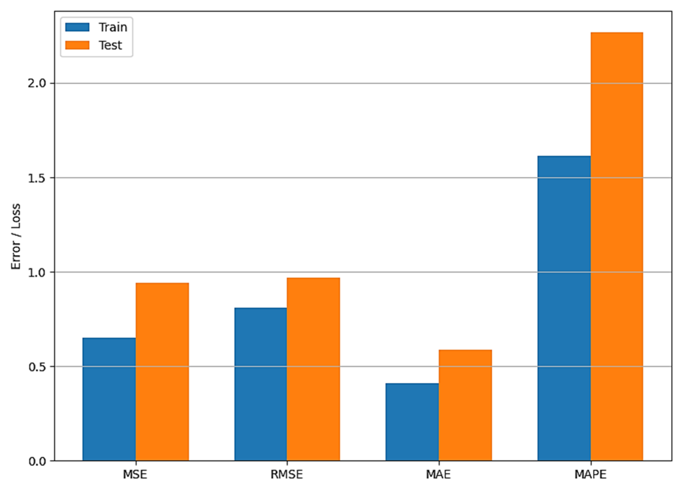
The RF model’s performance was assessed using 10-fold cross-validation in addition to the training dataset. The RF model demonstrated excellent predictive accuracy (R² = 0.93) on the training data. The model also demonstrated low errors, with MAE = 0.59, MAPE = 2.27%, MSE = 0.94, and RMSE = 0.97, further validating its accuracy and resilience. The RF model also performed well in 10-fold cross-validation, with a slightly lower R² of 0.90, suggesting its robustness and generalizability across multiple data subsets. In this process, the error matrices MAE and MAPE increased to 0.65 and 2.63%, indicating a modest rise in prediction error as the model was tested on diverse datasets. Similarly, the MSE and RMSE also climbed to 1.39 and 1.18, respectively, indicating that while the model performed slightly lower on unknown data, its generalization ability remained high. These findings support the RF model’s ability to predict concrete CS with high accuracy and consistent generalization across several validation techniques.

Figure 22 demonstrates possible overfitting of the RF model in terms of statistical errors, i.e., MSE, RMSE, MAE, and MAPE of training vs. testing errors. The findings demonstrate that while the test errors are somewhat higher than the training errors, the difference is not statistically significant, showing that the model generalizes efficiently and does not overfit the training data. In particular, the MSE and RMSE values for both the training and test datasets are quite comparable, whereas the MAE and MAPE exhibit a moderate rise in the test error. However, this discrepancy falls within an acceptable range and does not indicate serious overfitting. Overall, the model shows a high degree of generalization to unknown data, validating its reliability.

4.9. SHAP Analysis

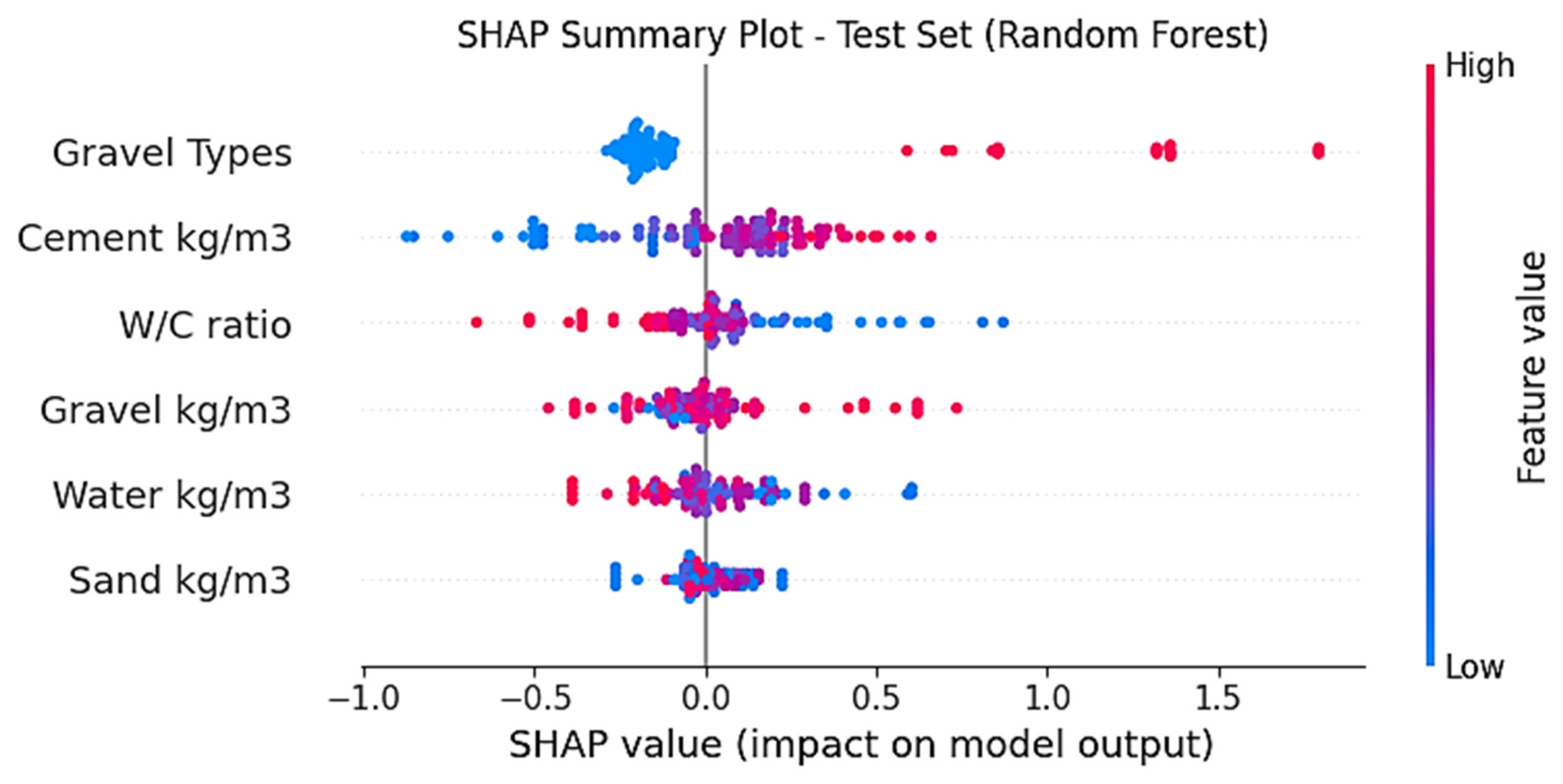
SHAP analysis was performed on the trained RF model. The SHAP analysis shown in Figure 23 indicates the relative relevance of input parameters in forecasting CS and how feature value variations affect the model output. The color of each point indicates whether the feature value is high (red) or low (blue), and each point represents a SHAP value for a test-set sample. Positive SHAP numbers correspond to gains in anticipated strength, whereas negative ones indicate declines in CS.

The combination of ML models with SHAP interpretability analysis provides more insight into the governing elements controlling CS. SHAP findings revealed that gravel type, cement concentration, and W/C ratio had a significant effect on CS prediction, agreeing closely with the measured experimental patterns. On the other hand, it was found that changes in the amounts of CA, water, and sand had relatively little impact on the CS. These findings validate the dependability and physical consistency of the suggested data-driven framework by showing that the ML models not only attained excellent predicted accuracy but also functioned in complete accordance with proven material behavior.

4.10. Feature Importance Analysis

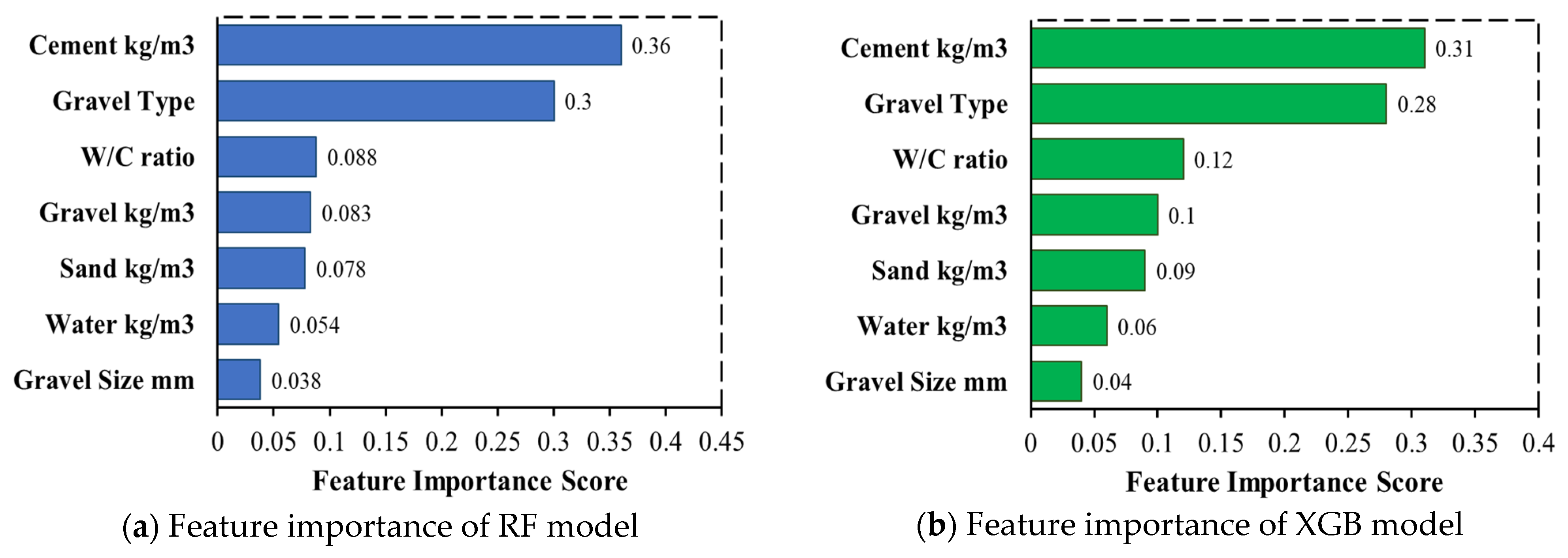
The feature importance analysis (FIA) is crucial for understanding the factors that significantly influence the CS of concrete. This section evaluates the results of the FIA, which was conducted using the ensembled models, i.e., RF and XGB. The RF and XGB models are particularly suitable for such analysis due to their ability to handle nonlinear relationships and interactions between features. The feature importance graphs, as shown in Figure 24a,b, provide a visual representation of the relative significance of various features in predicting the CS of concrete. The FIA of both models consistently emphasize the importance of cement content and gravel type, with minor contributions from water, sand, gravel volume, and W/C ratio in determining the CS of concrete.

In the RF, cement content was identified as the most influential factor with an importance score of 0.36. This finding highlights the critical role of cement content in the concrete mix, as it directly contributes to the hydration process, binding properties, and overall strength progression of concrete. Following closely, the gravel types parameter holds the second-highest importance score of 0.30. This indicates that the gravel type used in the concrete mix, whether natural or basalt significantly impacts its CS. The distinction between natural and basalt CA is particularly noteworthy, as it impacts the particle packing, ITZ, and load-bearing capacity. The W/C ratio (importance score = 0.09) is another critical factor influencing the CS of concrete. The w/c ratio is a well-established parameter that affects the porosity, workability, and strength of concrete. A lower w/c ratio generally results in higher CS, as it reduces the concrete porosity and enhances the density of the cement paste. However, an excessively low w/c ratio can lead to difficulties in mixing and placing the concrete, highlighting the need for careful optimization of this parameter. The amount of gravel recorded an importance score of 0.083, further emphasizing the significance of the aggregate content in the concrete mix. Gravel (kg/m³) plays a vital role in concrete’s mechanical and physical properties. Proper gravel grading and distribution are important for a dense, well-compacted concrete mix which is crucial for attaining high CS. Other components like sand content and water content, with importance scores of 0.078 and 0.054, showed moderate impact on the CS of concrete. Likewise, the XGB model supported similar results, identifying the main contributors as cement (importance = 0.31) and gravel type (importance = 0.28), followed by W/C ratio (0.12), sand (0.10), gravel content (0.09), water (0.06), and gravel size (0.04), respectively. The overall ranking pattern was quite constant, even if the importance scores varied slightly across the two models because of algorithmic differences in how splits and residuals are optimized.

The alignment of findings from the two ensemble ML models offers compelling support that cement content and gravel type are the main factors influencing concrete’s CS, while the W/C ratio acts as an essential regulating variable. The comparatively minimal impact of sand, gravel quantity, and water indicates that these factors serve more as supportive elements, affecting mixture stability and workability instead of having a direct effect on strength. The FIA clearly shows that ensemble-based machine learning models effectively capture the hierarchical contributions of mixed ingredients, offering strong interpretability that is consistent with domain knowledge. This confirms model stability and boosts confidence in predictive modeling and mix design optimization.

4.11. Graphical User Interface Development for Concrete Strength Prediction

An interactive graphical user interface (GUI) application was created to improve the usefulness of ML predictions for estimating the 28-day CS of NSC. For civil engineers, this application is a useful decision-support tool that enables rapid CS prediction based on CMD proportions. This optimizes material use, reduces trial costs, and makes on-site quality monitoring easier. In research contexts, predictive models like gradient boosting and RF provide reliable findings; however, their incorporation into an easily accessible interface helps to close the gap between advanced calculation and routine engineering practice.

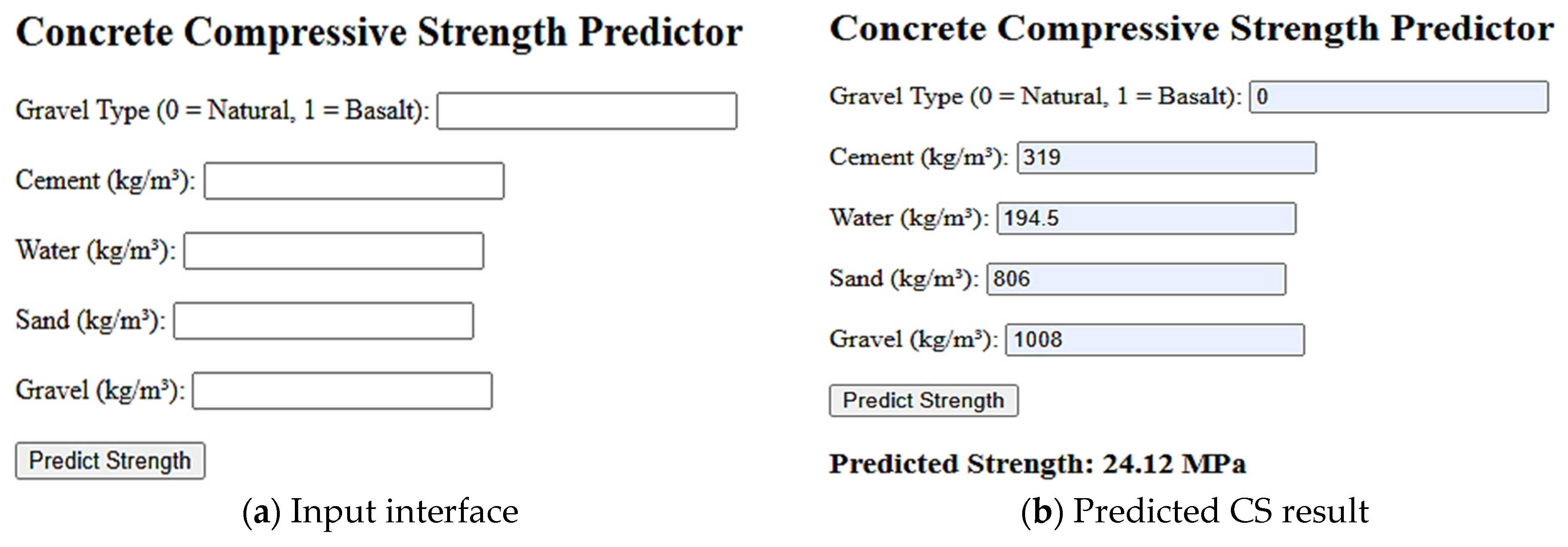
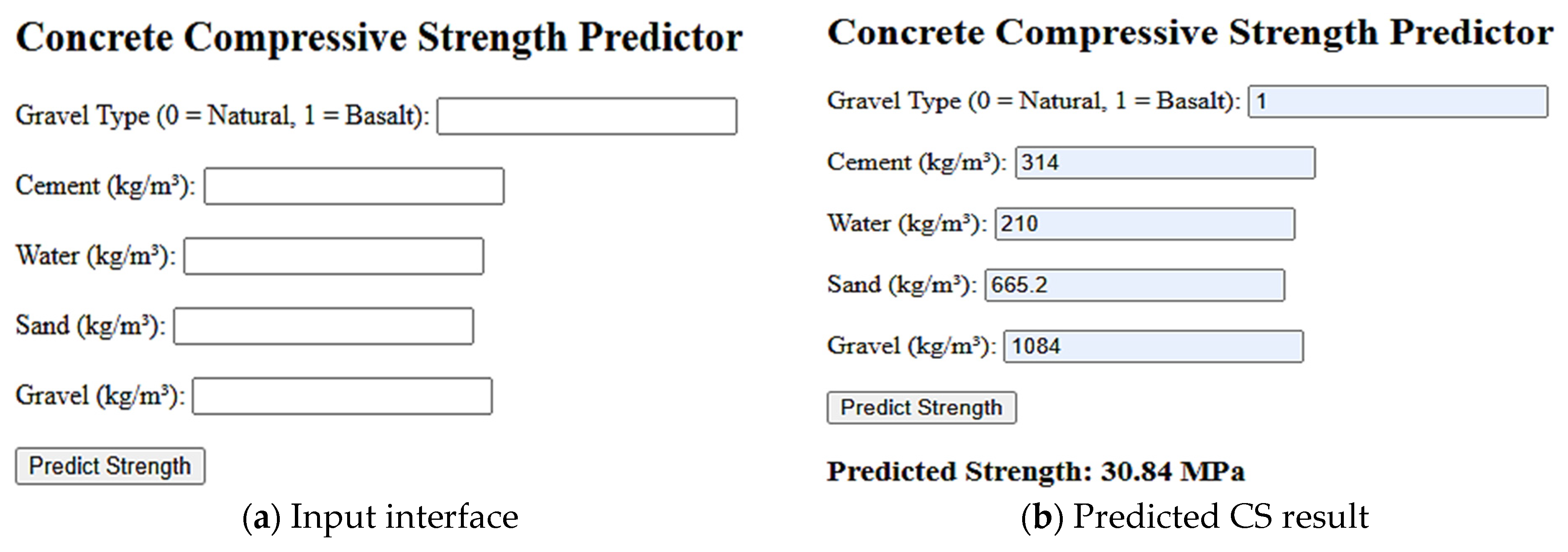
This application was developed in Python using pandas/numpy for data preparation, scikit-learn for model integration, and Tkinter/Streamlit for GUI. The process initiates with the user inputting specific parameters for the concrete mixtures in kg/m³ through dedicated entry fields of the GUI. The RF- and GB-trained ML models receive and process these inputs in real time. The ML trained models provide the expected 28-day CS after being refined and verified by cross-validation and hyperparameter adjustment. The GUI program, which can be seen in Figure 25 and Figure 26, allows the user to enter values for CMD ingredients such as cement, water, sand, gravel, W/C ratio, and gravel type. The prediction output screen then provides the estimated 28-day CS of concrete.

The GUI prediction tool’s applicability domain corresponds to the parameter ranges of the dataset used for development and training of the ML models, including cement content (288–375 kg/m³), sand content (600–806 kg/m³), gravel content (1000–1210 kg/m³), water content (170–210 kg/m³), W/C ratios (0.50–0.66), and CA type (natural 0, basalt 1). Predictions made outside of these ranges may not be reliable. The program produces compressive strength predictions for mixtures that generally range between 18 and 35 MPa, which is consistent with the experimental dataset. The users can easily access the tool by using the link https://huggingface.co/spaces/Sufianseu/Concrete-Strength-Predictor (accessed on 7 December 2025).

The created GUI tool is designed for practical usage in a variety of technical disciplines. Field engineers can easily use the GUI tool to predict concrete CS based on real-time mix parameter inputs during trial batching or site modifications, allowing for faster decisions about ingredient adjustments or replacements. Before conducting laboratory experiments, design engineers can utilize the tool during preliminary mix proportioning to assess the impact of changing cement content, W/C ratio, and aggregate type on the final strength. Technicians at quality control labs can utilize the GUI to compare strength results specified by various CMD codes and to verify mix uniformity across concrete batches. Additionally, the program offers researchers a handy way to examine parametric variations without performing repetitive, laborious computations.

To validate the practical utilization of the developed GUI tool, two demonstrations were performed by comparing the predicted CS from the GUI tool with actual experimental CS. Figure 25 represents the ACI CMD of natural CA (ACI-N15) and the GUI-predicted CS is 24.12 MPa, which is in close agreement with the experimental CS of 24.1 MPa. Figure 26 represents the JGJ CMD of basalt CA (JGJ-B15). In this case, the GUI tool predicted the CS as 30.84 MPa, which is consistent with the experimental CS of 30.7 MPa. These comparisons demonstrate the tool’s capacity to reliably forecast compressive strength and validate its value for optimizing concrete mix designs in real-world circumstances.

4.12. Practical Engineering Implications

The findings of this study offer several practical insights for engineering practices such as structural performance, concrete production, quality control operations, and a user-friendly CS prediction tool. The incorporation of crushed basalt CA significantly improved CS, stiffness, and energy accumulation (G_A and G_F) of concrete, indicating their potential for structural components needing increased mechanical dependability and post-peak behavior. In terms of CMD, the comparative analysis of ACI, BS, IS, and JGJ codes demonstrates how differences in proportioning, especially in cement content, W/C ratio, and CA type can affect mechanical results; this offers engineers important guidance when choosing CMD standards for particular performance goals.

The use of ML models in the research offers engineers a practical tool to accurately forecast the 28-day CS of concrete. This predictive ability has the potential to streamline design workflows and enhance quality assurance efforts. The application of this technique allows engineers to reduce trial-and-error testing, accelerating construction deadlines while maintaining structural integrity.

The development of a user-friendly GUI tool for real-time concrete strength prediction utilizing ML models marks an advancement in real-world engineering applications. This strength prediction tool can simplify on-site decision-making and optimize the mix design process, minimizing the need for costly and lengthy laboratory testing and enabling field and design engineers to make faster, data-driven judgments in CMD. The findings of this study provide significant insights into the enhancement of concrete’s mechanical properties, the advancement of sustainability, and cost efficiency in contemporary construction practices.

5. Future Recommendations and Limitations of the Study

Future studies should evaluate the long-term durability performance of the assessed CMD codes and basalt CA under different exposure conditions to further validate the findings of this study. Additionally, future research may investigate deep learning approaches for modeling higher-dimensional features and complex nonlinear relationships of concrete. In order to more accurately link CA shape to strength development and failure responses, future research should include quantitative aggregate morphology assessments, such as ASTM D4791 flakiness and elongation indices or image-based angularity metrics, and petrographic analysis. Further generalization of the findings would also be possible by extending the range of aggregate sizes, cement types, and strength classes.

This investigation is limited to a single CA size and one type of cement, which may limit its direct applicability to different CA sizes or types of cement. The results of this study may not be entirely applicable to HSC classes since the experimental matrix was restricted to NSC. The ML models and GUI tool are trained within the current dataset’s parameter ranges; predictions made beyond these limits may result in lower dependability. In the next project, the materials’ variability and concrete strength range will be expanded to improve the generalization and applicability of the results.

6. Conclusions

The experimental investigations of this study evaluated the influence of coarse aggregate (CA) type, shape, and specimen configuration on the compressive behavior of NSC. Concrete mixtures were prepared using basalt and natural CA according to four CMD codes and tested using various specimen geometries to assess failure modes, compressive strength (CS), energy accumulation (GA), and fracture energy (GF). Four machine learning (ML) algorithms were also developed to validate the experimental findings and predict the 28-day CS. Based on the experimental and ML model results, the following conclusions are drawn:

• Basalt CA concrete consistently exhibited superior mechanical performance compared to natural CA concrete across all CMD codes and specimen sizes, emphasizing the importance of CA mineralogy, surface texture, and morphology in determining strength and toughness.
• The specimen configuration influenced the compressive behavior of concrete, with larger cylindrical specimens demonstrating enhanced strength and energy-related parameters. This highlights the size-dependent response of concrete that should be considered when assessing structural performance.
• The performance of basalt CA concrete remained consistent across CMD codes, suggesting that CA type and grading should be treated as key design variables, alongside binder content and water-to-cement ratio control.
• Tree-based ensemble ML models, particularly Random Forest and gradient boosting methods, provided reliable predictions of 28-day CS and effectively captured nonlinear relationships between mix design variables and concrete strength.
• Feature importance analysis and SHAP analysis identified cement content and CA type as the most influential contributors to CS, followed by water-to-cement ratio as a crucial regulator. These findings align with established material behavior theories related to hydration, porosity control, and ITZ characteristics.
• A Python-based graphical user interface (GUI) tool was developed to facilitate immediate, mix-specific strength estimation. This tool enhances decision-making in concrete design by reducing reliance on extensive laboratory testing.

In summary, the study demonstrates that CA type and specimen geometry play significant roles in shaping the mechanical behavior of NSC. Basalt CA provides clear improvements in strength and post-peak behavior, while ensemble ML models offer strong predictive capability and interpretability. The integrated experimental–ML framework and the developed GUI tool together support more efficient and data-driven concrete mix design and quality control.