Research on a Comprehensive Performance Analysis Method for Building-Integrated Photovoltaics Considering Global Climate Change

Abstract

Building-integrated photovoltaics (BIPVs) represent a pivotal technology for enhancing the utilization of renewable energy in buildings. However, challenges persist, including the lack of integrated design models, limited analytical dimensions, and insufficient consideration of climate change impacts. This study proposes a comprehensive performance assessment framework for BIPV that incorporates global climate change factors. An integrated simulation model is developed using EnergyPlus8.9.0, Optics6, and WINDOW7.7 to evaluate BIPV configurations such as photovoltaic facades, shading systems, and roofs. A multi-criteria evaluation system is established, encompassing global warming potential (GWP), power generation, energy flexibility, and economic cost. Future hourly weather data for the 2050s and 2080s are generated using CCWorldWeatherGen under representative climate scenarios. Monte Carlo simulations are conducted to assess performance across variable combinations, supplemented by sensitivity and uncertainty analyses to identify key influencing factors. Results indicate (1) critical design parameters—including building orientation, wall thermal absorptance, window-to-wall ratios, PV shading angle, glazing optical properties, equipment and lighting power density, and occupancy—significantly affect overall performance. Equipment and lighting densities most influence carbon emissions and flexibility, whereas envelope thermal properties dominate cost impacts. PV shading outperforms other forms in power generation. (2) Under intensified climate change, GWP and life cycle costs increase, while energy flexibility declines, imposing growing pressure on system performance. However, under certain mid-century climate conditions, BIPV power generation potential improves due to altered solar radiation. The study recommends integrating climate-adaptive design strategies with energy systems such as PEDF (photovoltaic, energy storage, direct current, and flexibility), refining policy mechanisms, and advancing BIPV deployment with climate-resilient approaches to support building decarbonization and enhance adaptive capacity.

1. Introduction

Under the guidance of China’s “Dual Carbon” strategy (carbon peak and carbon neutrality), building-integrated photovoltaics (BIPVs) have emerged as a critical pathway for facilitating the low-carbon transformation of the building sector. At the policy level, explicit targets have been set to achieve a 50% coverage rate of photovoltaic systems on the roofs of new public buildings and factory buildings by 2025, alongside the encouragement of maximizing installations on existing building roofs wherever feasible. Concurrently, the technical standard system related to BIPV continues to be refined, with numerous regions promoting its large-scale implementation through technical guidelines, pilot projects, and financial subsidies. Driven by the synergistic effects of policy, standardization, and practical application, BIPV is rapidly evolving from a forward-looking technology into a key solution for constructing low-carbon cities and advancing the transformation of the energy structure.

Among the application forms of building-integrated photovoltaics (BIPVs), façade integration primarily encompasses three major categories: photovoltaic curtain walls, photovoltaic windows, and photovoltaic shading systems, each achieving synergistic optimization of energy generation and building performance at distinct levels [1]. Among these, research on photovoltaic curtain walls predominantly focuses on the comprehensive effects of panel orientation, tilt angle, and cavity structure on both building heat transfer and power generation performance [2]. For instance, Liu et al. [3] proposed a novel symmetrical pentahedral photovoltaic curtain wall, composed of a vertical façade, upper and lower inclined surfaces, and two side surfaces. By optimizing structural parameters such as the opening angle of the upper inclined surface, the convex horizontal side length ratio, and the extension length, they significantly enhanced the power generation efficiency per unit area. Compared to traditional vertical BIPV curtain walls, this design demonstrates significant improvement in annual power generation across different orientations, with the most pronounced enhancement reaching 104% in the west-facing scenario. Research on photovoltaic windows primarily focuses on the performance of various semi-transparent photovoltaic materials in regulating indoor daylighting and reducing cooling loads, thereby balancing visual comfort with energy-saving potential [4]. For instance, Li et al. [5] proposed a novel photovoltaic energy-saving window (PEW), composed of laterally slidable CdTe photovoltaic glass, a retractable polyurethane insulation shade in the middle, and an inner layer of double-pane transparent glass. Their investigation into the influence of parameters such as the number of transparent glass layers, thickness of the insulation shutter, number of photovoltaic glass layers, and light transmittance on building heating load revealed that the PEW reduced the annual heating load by 23.54% compared to double-pane transparent glass and by 15.42% compared to triple-pane transparent glass. Photovoltaic shading systems, through geometric optimization and dynamic control, enhance photovoltaic efficiency while fulfilling their shading function and improving the indoor photothermal environment [6]. For example, Ye et al. [7] integrated photovoltaic modules into building shading structures, enabling on-site power generation while blocking excessive sunlight. Utilizing a GIS-based spatiotemporal analysis and multi-objective optimization method, their study achieved a 57.40% increase in daily power generation efficiency per unit area compared to static horizontal installation. In summary, current research has independently advanced various BIPV technologies from the perspectives of structural design, material performance, and system control. However, the deep integration between photovoltaic systems and passive building energy-saving design has not yet been fully realized. Integrated modeling and the synergistic optimization mechanism for multiple performance aspects remain areas requiring further exploration.

In research on the performance optimization design of BIPV systems, existing studies have extensively elucidated the coupling mechanisms between photovoltaic design and the building’s physical environment. Specifically, current research focuses on systematically analyzing how key parameters—such as the arrangement of photovoltaic panels as building envelopes, shading coefficients, and light transmittance—comprehensively influence building thermal performance in both winter (insulation) and summer (heat mitigation), and consequently affect visual comfort indicators, including indoor illuminance and glare probability [8]. The core objective is to achieve multi-objective synergy and global optimization among building energy production, energy-saving benefits, and occupant comfort [9]. For instance, Wijeratne et al. [10] employed the NSGA-II multi-objective optimization algorithm to optimize both the life cycle cost and life cycle energy output of BIPV roof systems. Their approach identified optimal solutions for rooftop BIPV panels and skylight BIPV configurations, streamlining the process of identifying economically viable and highly efficient design solutions during the early project stages. Chen et al. [11] integrated transfer learning, the NSGA-III genetic algorithm, and CFD simulations into a multi-objective optimization framework to enhance multidimensional performance of photovoltaic façades in educational buildings, including carbon emissions, power generation, indoor lighting, and thermal comfort. Their optimal solution achieved a reduction in carbon emissions of 27.5 kgCO₂/m². Sadatifar et al. [12] applied a Monte Carlo-based stochastic optimization method to iteratively optimize three key parameters of photovoltaic shading panels—tilt angle, length, and quantity—across five climate zones and two building types. This approach realized synergistic optimization of “power generation–energy saving–comfort,” providing a feasible pathway for the customized design of BIPV systems in diverse contexts. Bakmohammadi et al. [13] integrated a deep learning model for façade segmentation with a multi-objective optimization algorithm to optimize three sustainability dimensions of building-integrated photovoltaic façades: energy self-sufficiency rate, economic payback period, and life cycle greenhouse gas emission rate. Their results demonstrated that the optimal solution under balanced weighting could achieve an electricity self-sufficiency rate of 5% to 7%. It should be noted, however, that with the emergence of new technologies such as grid-interactive functionalities, indicators such as energy flexibility must also be incorporated during the design phase, as they significantly influence the system’s grid interaction capability in actual operation. The aforementioned study, along with others, lacks comprehensive consideration of integrated factors including power generation capacity, carbon emissions, and energy flexibility. Nevertheless, with the rise of grid-interactive technologies and other innovations, the role of BIPV systems is evolving from that of a passive energy producer to an active grid supporter and flexible resource [14]. This shift necessitates the proactive inclusion of emerging performance metrics, such as energy flexibility, already at the design stage, since early design decisions directly determine the system’s future grid interaction capability and carbon reduction potential in real-world operation [15]. However, existing research predominantly focuses on balancing thermal and visual comfort performance, and still lacks a comprehensive design framework capable of coordinating multiple objectives such as power generation capacity, life cycle carbon emissions, and energy flexibility. This research gap substantially limits the potential of BIPV systems to maximize their role in achieving building-grid synergy and fulfilling the “Dual Carbon” goals.

In current research on performance simulation and uncertainty analysis of building-integrated photovoltaics (BIPVs), meteorological parameter uncertainty has garnered significant attention; however, predominant evaluation methodologies exhibit notable limitations. Most existing approaches rely on typical meteorological year (TMY) data or “typical day” sequences derived from historical weather data, which primarily capture short-term meteorological variations (e.g., hourly, daily, weekly, or seasonal fluctuations) but systematically fail to incorporate the annual weather changes driven by global warming [16]. For instance, Wang et al. [17] utilized TMY data to conduct annual hourly simulations, performing a comparative analysis of three BIPV systems—photovoltaic roofs, photovoltaic windows, and photovoltaic shading—to evaluate their energy performance and load-matching characteristics across different climate zones. Tang et al. [18] employed TMY data incorporating urban heat island effects, combined with a three-dimensional local climate zone (LCZ) model and machine learning techniques, to assess the annual power generation potential of urban rooftop and façade BIPV systems and quantify the nonlinear relationships between urban morphological factors, climatic conditions, and system performance. Similarly, Xu et al. [19] applied Hong Kong TMY data to analyze how geometric and color parameters affect the power generation efficiency and total output in a composite solar façade system comprising photovoltaic walls and shading elements. Their results demonstrated that photovoltaic shading achieves higher generation efficiency than photovoltaic walls under more favorable solar incidence angles. Zou et al. [20] developed a novel dynamic vertical building-integrated photovoltaic envelope system, which adaptively adjusts slat angles and louver positions to simultaneously optimize power generation, daylighting, and thermal load regulation. Using typical seasonal day and annual meteorological data for Beijing in their simulation analysis, the study demonstrated that this dynamic configuration could increase the annual net energy output by at least 226% compared to conventional static photovoltaic shading systems. However, this prevalent neglect of long-term climatic dynamics directly compromises the accuracy of life cycle performance assessments and operational effectiveness of BIPV systems. For instance, Wang et al. [21] highlighted through a coupled analytical framework that climate change-induced extreme events—such as prolonged periods of low wind and solar availability—significantly elevate levelized electricity costs and power supply demand imbalance risks. If such year-to-year changing factors are not considered during the design phase, BIPV design strategies will lack foresight, thereby undermining their long-term climate adaptability and operational reliability. In summary, prevailing uncertainty assessments for BIPV systems remain largely confined to short-term meteorological fluctuations and static climate assumptions. To enhance the resilience of BIPV buildings in future warming environments, it is imperative to integrate climate scenario data reflecting long-term trends into performance simulations and to establish a new uncertainty assessment framework that incorporates interannual temporal analysis. Such advancements are essential to support the low-carbon, robust operation and sustainable adaptation of BIPV systems over their full life cycle.

2. Materials and Methods

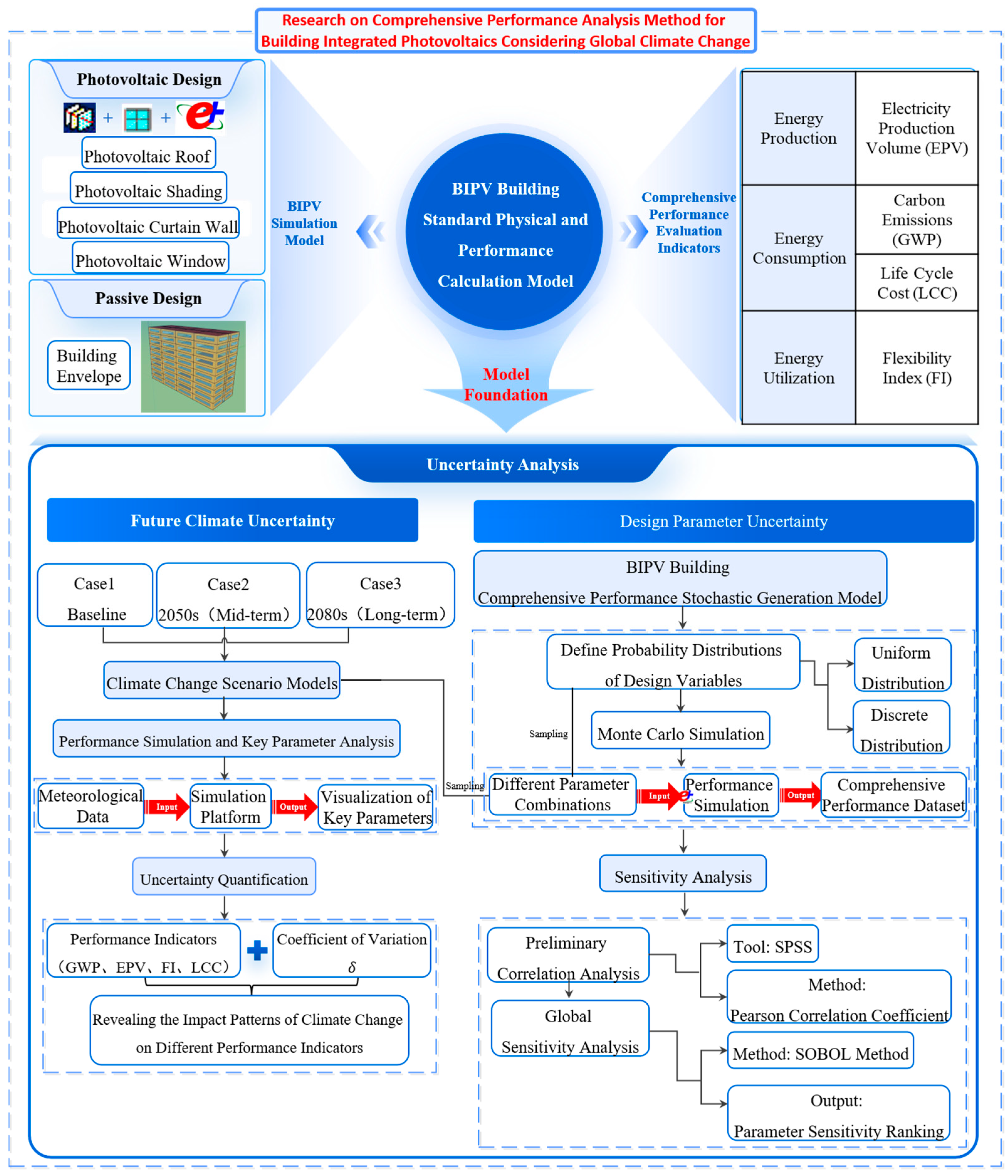
The analytical methodology proposed in this study comprises five core components, as illustrated in Figure 1: (1) An integrated simulation model suitable for photovoltaic curtain walls, photovoltaic shading systems, and photovoltaic roofs was developed by coupling EnergyPlus, Optics6, and WINDOW 7.7 software. (2) A comprehensive performance evaluation indicator system was established, encompassing four dimensions: carbon emissions, power generation, energy flexibility, and economic cost. (3) Utilizing the CCWorldWeatherGen tool, hourly meteorological data incorporating future climate scenarios were generated, covering two time periods: the 2050s and the 2080s. (4) Based on the Monte Carlo method, batch simulations of BIPV performance were conducted for various combinations of design variables and under different climate scenarios. (5) Sensitivity analysis and uncertainty analysis methods were applied to identify key influencing factors and reveal the impact patterns of climate change on different performance indicators.

2.1. Building-Integrated Photovoltaic Simulation Model

The primary objective of this study is to develop a building-integrated photovoltaic (BIPV) simulation model for parametric analysis and predicting future performance trends, rather than accurately replicating the actual energy consumption of specific buildings. Under this research objective, this paper follows the typical paradigm in the field, primarily relying on simulation software to obtain building performance data without conducting specific experimental validation. The validity of this approach has been corroborated by numerous similar studies: for instance, Gomes et al. used EnergyPlus to simulate building energy consumption and thermal comfort data to evaluate the performance improvement of residential renovation solutions in Portugal [22]; Chen et al. employed a co-simulation of EnergyPlus and BCVTB to provide operational data for developing solar integration control strategies [23]; Gasparella et al. utilized EnergyPlus to analyze the impact of different extreme weather data on building energy performance [24]. These studies all focus on exploring the performance and behavioral mechanisms of complex systems through mature and widely validated simulation tools. Therefore, the simulation results obtained under specific scenarios, based on recognized and reliable simulation platforms, possess the scientific rigor and reliability necessary to support subsequent parametric analysis and trend inference in this study [25].

2.1.1. Architectural Model

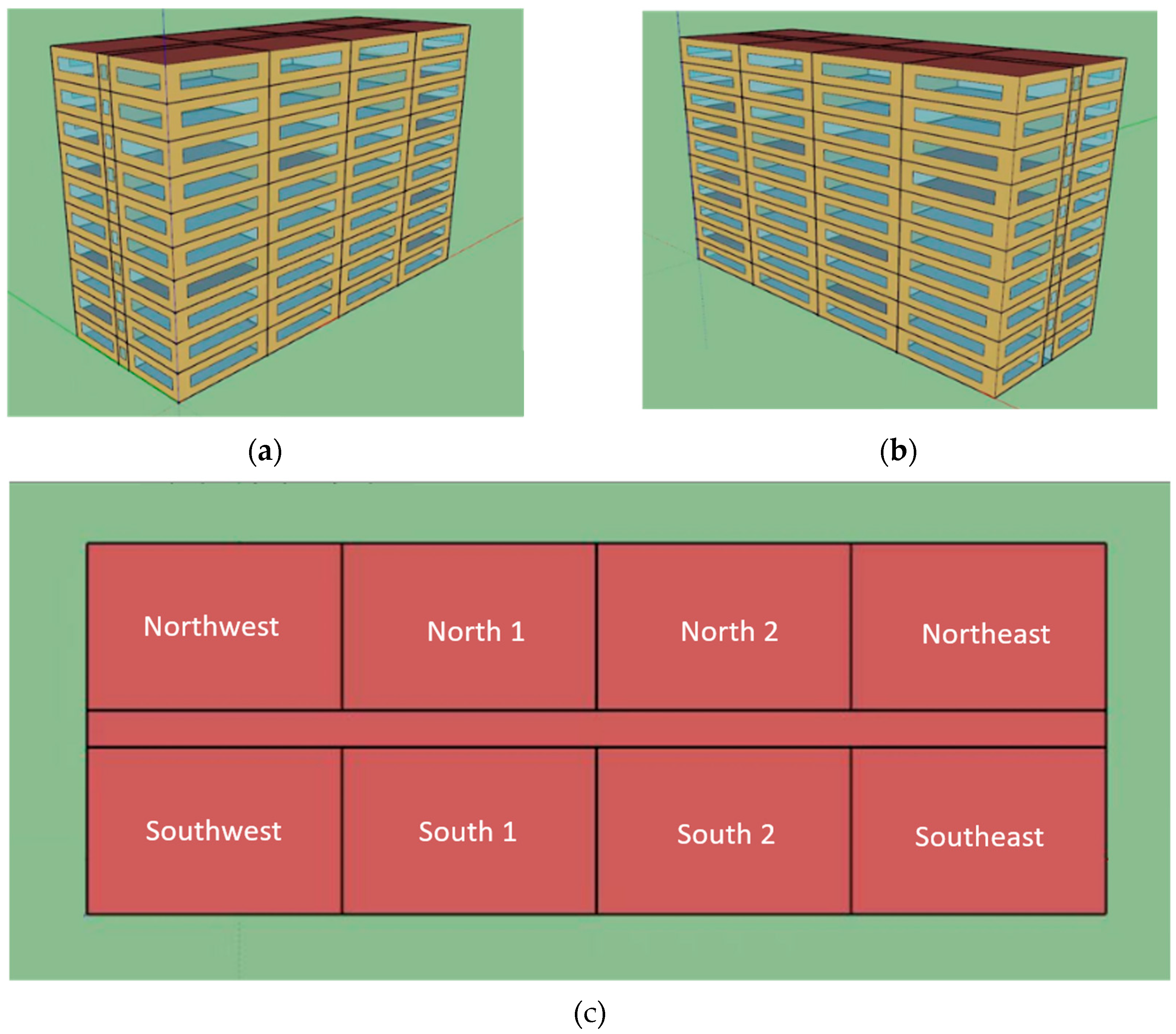
The U.S. Department of Energy (DOE) and the Pacific Northwest National Laboratory (PNNL) have jointly developed a prototype building model library encompassing commercial, residential, and office buildings. The prototype buildings within this library can serve as reference benchmarks for new construction projects after limited modifications [26]. This study used a high-rise residential building compliant with ASHRAE Standard 90.1 as the reference case. The building model, depicted in Figure 2, represents a high-rise apartment building. To account for the integration of photovoltaic components into the building façade and the incorporation of external shading strategies, the original model was adapted by adding external shading panels to the south-facing elevation. Detailed parameters of the building are provided in

Table 1. BIPV building’s detailed information.

Building Model	Northwest	North 1	North 2	Northeast	Southwest	South 1	South 2	Southeast
Aspect Ratio	2.75
Shape Coefficient	0.227
Number of Floors	10
Floor Area	8640
Story Height (m)	3
Window Height (m)	0.95
Shading	None				External Shading, 8.7 m × 1 m
Thermal Zone	Floors 1–10: Residential	Floors 1–10: Residential	Floors 1–10: Residential	Floors 1–10: Residential	Floors 1–10: Residential	Floors 1–10: Residential	Floors 1–10: Residential	1F: Office, Floors 2–10: Residential

.

To clarify the fundamental inputs of the simulation and enhance the verifiability of the model, this study provides detailed specifications for the building’s internal loads and HVAC system. The specific settings are as follows:

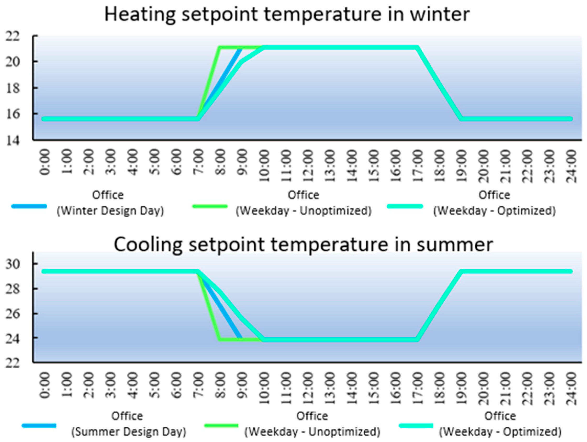
HVAC System: the heating setpoint for residential areas during occupancy hours is 21.7 °C, while the cooling setpoint is 24.4 °C. For office areas, temperature setpoints are adjusted using a time-dependent strategy based on their complex occupancy patterns (see Figure 3 for details).

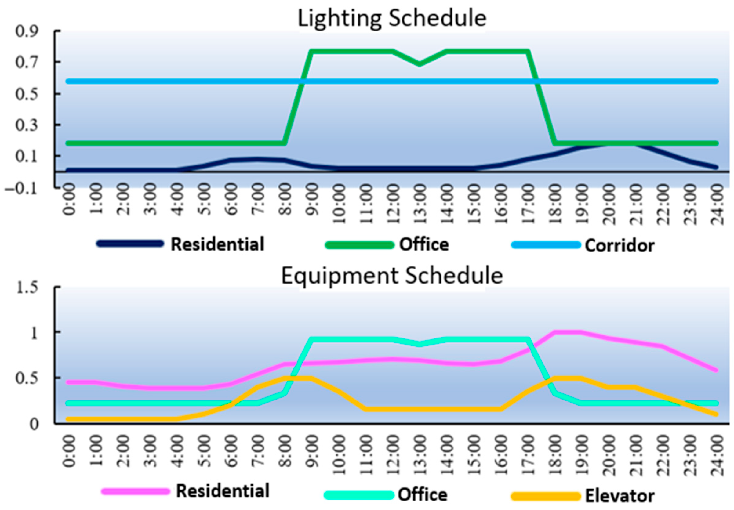
Lighting and Equipment: the lighting power density in each area is set according to its function, with residential areas at 6.45 W/m², offices at 7.96 W/m², and corridors at 5.29 W/m². Additionally, the electrical equipment power density for both offices and residential areas is set at 6.67 W/m². The elevator equipment power is configured at 20,370 W, and the fan power is set at 63 W. The operation of all lighting and equipment is controlled based on predefined schedules (see Figure 4 for details).

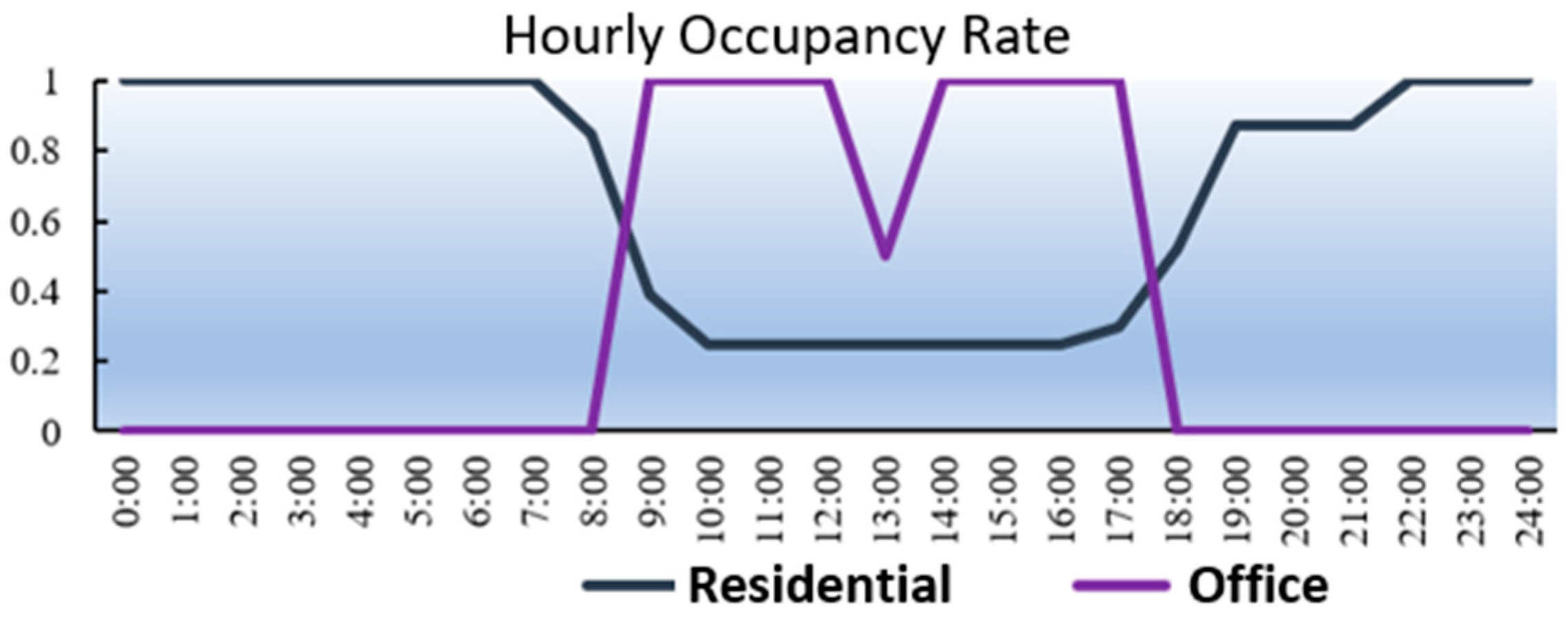
Internal Heat Gains: the occupant density is set at one person per 25 m² for residential areas and five persons per unit area for offices. The hourly occupancy rate is also simulated based on a predefined schedule (see Figure 5 for details).

Simulation Time Step: EnergyPlus simulation adopts the default time step settings to ensure a balance between computational efficiency and accuracy.

2.1.2. Photovoltaic System Model

This study employed Optics6 and WINDOW 7.7, developed by Lawrence Berkeley National Laboratory (LBNL), to simulate the performance of photovoltaic modules, while their power generation performance was modeled using the Sandia model integrated in EnergyPlus. Specifically, WINDOW 7.7 was utilized to determine the optical and thermal properties of window systems [27], and Optics6 was applied to calculate the transmittance and reflectance of photovoltaic modules across solar and visible light spectra [28]. For power generation simulation, south-facing photovoltaic shading panels and rooftop photovoltaic components utilized component database files from the System Advisor Model (SAM) PV-Component library [29]. In contrast, the power generation performance of east–west-oriented photovoltaic windows and north-facing photovoltaic walls was simulated based on validated data from existing literature. SAM, developed by the National Renewable Energy Laboratory (NREL), provides a detailed parameter database encompassing recently manufactured and tested photovoltaic modules and inverters.

1.

Photovoltaic roof

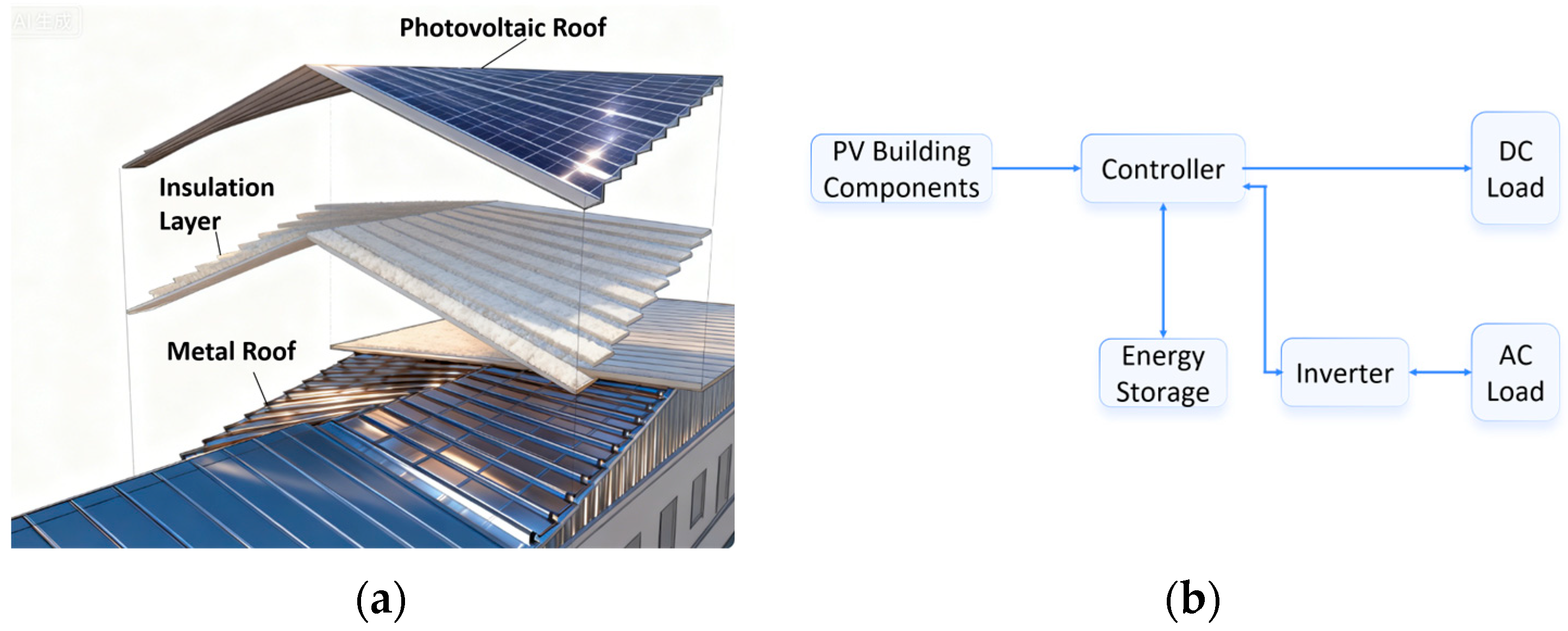
The photovoltaic-integrated roof system in this study utilizes the Silevo Triex U300 Black high-efficiency monocrystalline silicon module from the Sandia PV data database. The manufacturer of the Silevo Triex U300 Black is Silevo (a subsidiary of SolarCity/Tesla), with its headquarters located in San Jose, California, United States. The system construction integrates photovoltaic components as a functional layer with conventional roofing to form a unified building envelope. Furthermore, based on the dimensions and layout of the roof installation area, corresponding series–parallel electrical connections were configured to establish the photovoltaic array. A key feature of this integrated solution is the addition of a photovoltaic layer above conventional construction, which serves dual functions of power generation and heat transfer. The relevant photoelectrical parameters are detailed in

Table 2. Electrical characteristics of the Sandia model.

Parameter	Unit	Silevo_Triex_U300_Black	SolarWorld Sunmodule 250 Poly
Usable Area	m2	1.68	1.68
Number of Modules in Series	Units	96	60
Number of Modules in Parallel	Units	1	1
Short-Circuit Current	A	5.771	8.3768
Open-Circuit Voltage	V	68.5983	36.3806
Current at Maximum Power Point $I_{mp}$	A	5.383	7.6921
Voltage at Maximum Power Point $V_{mp}$	V	55.4547	28.348
Temperature Coefficient of Short-Circuit Current ${\alpha }_{sc}$	1/K	0.0003	0.0006
Temperature Coefficient of Current at Maximum Power Point ${\alpha }_{mp}$	1/K	−0.003	−0.0001
Sandia Model Parameter C0		0.995	1.0158
Sandia Model Parameter C1		0.005	−0.0158
Temperature Coefficient at Maximum Power Point Voltage under Reference Conditions ${\beta }_{oc}$	V/K	−0.1913	−0.1393
Irradiance-Related Temperature Coefficient at Open-Circuit Voltage $m_{{\beta }_{oc}}$	V/K	0	0
Temperature Coefficient at Open-Circuit Voltage under Reference Conditions ${\beta }_{mp}$	V/K	−0.184	−0.1449
Irradiance-Related Temperature Coefficient at Open-Circuit Voltage $m_{{\beta }_{mp}}$	V/K	0	0
Diode Empirical Factor n		1.345	1.226
Sandia Model Parameter C2		0.3221	−0.09677
Sandia Model Parameter C3		−6.7178	−8.51148
Sandia Model Parameter a0		0.9191	0.9288
Sandia Model Parameter a1		0.09988	0.07201
Sandia Model Parameter a2		−0.04273	−0.02065
Sandia Model Parameter a3		0.00937	0.002862
Sandia Model Parameter a4		−0.00076	−0.00015
Sandia Model Parameter b0		1	1
Sandia Model Parameter b1		−0.0065	−0.00308
Sandia Model Parameter b2		0.000691	0.000405
Sandia Model Parameter b3		−2.7 × 10−5	−1.7 × 10−5
Sandia Model Parameter b4		4.32 × 10−7	3 × 10−7
Sandia Model Parameter b5		−2.51 × 10−0.9	−1.88 × 10−9
Thermal Voltage at Tc δ(Tc)		3.13	3.19
Diffuse Radiation Factor fd		1	1
Sandia Model Parameter a		−3.6866	−3.73
Sandia Model Parameter b		−0.104	−0.1483

, while the system configuration and power generation principle are illustrated in Figure 6.

2.

Photovoltaic Shading

Photovoltaic shading panels were installed on the exterior wall above all windows of the south-facing façade, with the specific installation configuration illustrated in Figure 7. The selected photovoltaic modules consisted of SAM high-efficiency multicrystalline silicon (mc-Si) components (SolarWorld Sunmodule 250 Poly, Manufacturer: SolarWorld Americas Inc., Hillsboro, OR, USA) from the SandiaPVdata database, which have been experimentally validated by Sandia National Laboratories [30]. Their performance parameters are provided in Table 2. To analyze the self-consumption of building electricity loads and photovoltaic power generation in the building-integrated system, a photovoltaic generator was integrated at the shading panel location.

The windows beneath the shading panels were constructed with double-pane Low-e glass selected from the EnergyPlus Window Glass Materials database, with a configuration of “3 mm clear glass + 6 mm air gap + 3 mm Low-e clear glass.” The optical and thermal properties of this glazing material are presented in

Table 3. Photothermal characteristics of low-e glass.

Parameter			Clear 3MM	LoE CLEAR 3MM Rev
Transmittance	Solar		0.837	0.63
	Visible Light		0.898	0.85
Reflectance	Solar	Front Plate	0.075	0.22
		Back Plate	0.075	0.19
	Visible Light	Front Plate	0.081	0.079
		Back Plate	0.081	0.056
Emissivity	Front Plate		0.84	0.1
	Back Plate		0.84	0.84
Thermal Conductivity			0.9	0.9

. Additionally, thermal performance parameters of the conventional double-pane window, calculated using WINDOW 7.8 software, are summarized in

Table 4. Heat transfer performance of double low-e windows [31]. Reproduced with permission from Shilei Lu, Hongcheng Zhu, Quanyi Lin, Yongjun Sun, Shengying Huang, Ran Wang, from Journal of Building Engineering, published by Elsevier, 2025.

Window	U-Value	SHGC	VLT
Dbl loe Clr 3 + 6 + 3 mm	2.4709	0.6365	0.7682

.

3.

Photovoltaic Curtain Wall

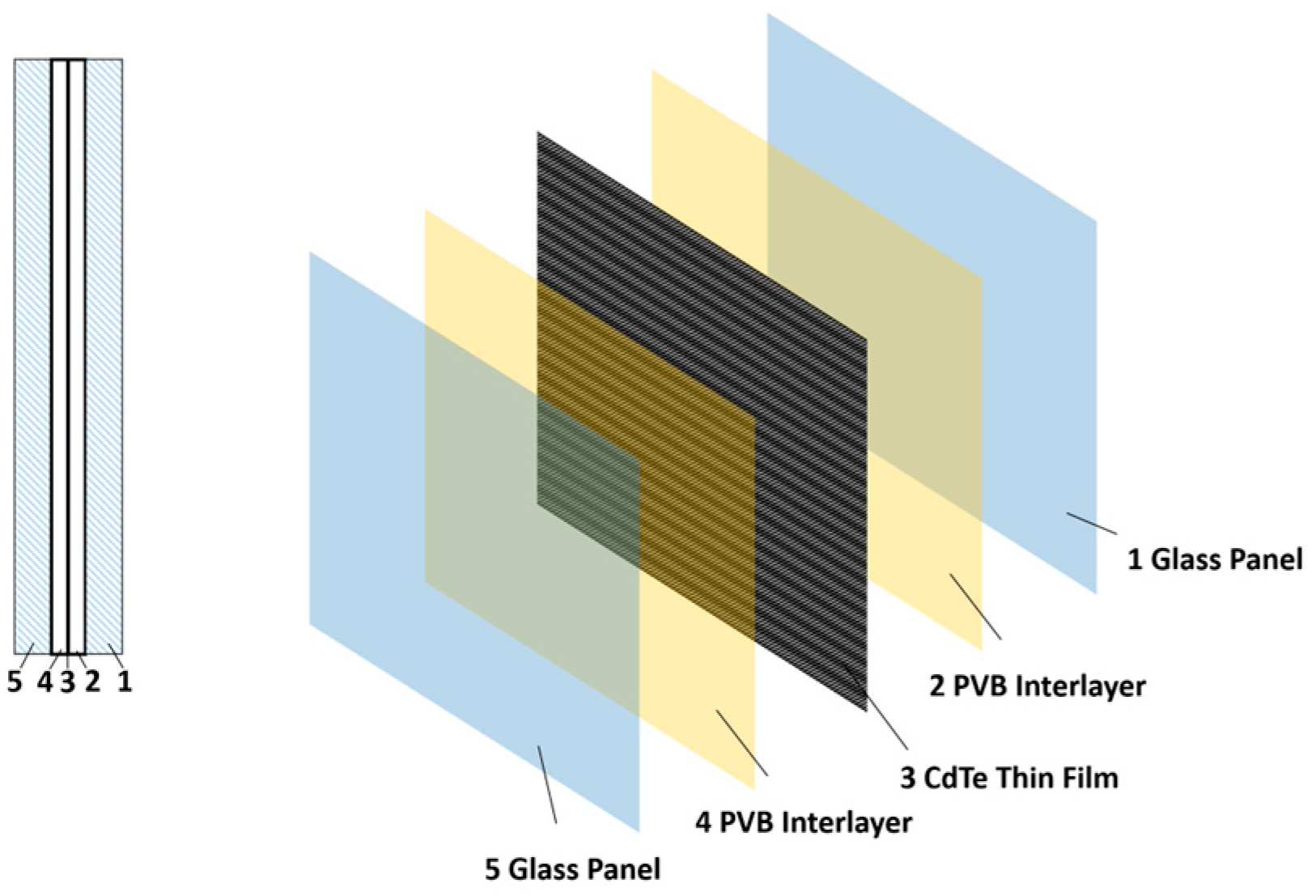
Photovoltaic modules can utilize various technologies, including monocrystalline silicon, polycrystalline silicon, and thin-film cells. Currently, semi-transparent photovoltaic components based on amorphous silicon (a-Si) and crystalline silicon have been extensively investigated, while cadmium telluride (CdTe) thin-film photovoltaic modules demonstrate significant research potential. Accordingly, this section employs CdTe thin-film technology to construct the north-facing photovoltaic wall, with its structural configuration illustrated in Figure 8. The visible light transmittance (250–2500 nm wavelength range) of this CdTe thin-film photovoltaic module is 12.3%. To simulate the power generation performance of the photovoltaic wall, a photovoltaic generator was incorporated into the system, with fundamental electrical characteristics provided by the manufacturer and detailed parameters listed in

Table 5. Characteristics of CdTe thin-film batteries in north-facing semi-transparent photovoltaic wall.

CdTe Thin-Film Battery	Transmittance 12.3%
Rated Power Pm/W	63.50
Short-Circuit Current Isc/A	0.78
Open-Circuit Voltage Uoc/V	116
Current at Maximum Power Imp/A	0.73
Voltage at Maximum Power Ump/V	87
Rated Efficiency η/%	8.8
Temperature Coefficient of Isc (%/°C)	0.06
Temperature Coefficient of Uoc (%/°C)	−0.321
Temperature Coefficient of Pm (%/°C)	−0.214

.

For photothermal performance characterization, the CdTe thin-film module referenced experimentally measured data from the literature [29], which were obtained using a PerkinElmer ultraviolet-visible-infrared spectrophotometer (located in Shelton, CT, USA) and a Hot Disk AB TPS 500 thermal constants analyzer (based in Gothenburg, Sweden). The photothermal characteristic parameters corresponding to the 12.3% transmittance CdTe cell are presented in

Table 6. Photothermal characteristic parameters of CdTe batteries.

Performance			Transmittance 12.3%
Transmittance	Solar		0.102
	Visible Light		0.123
Reflectance	Solar	Front Plate	0.082
		Back Plate	0.154
	Visible Light	Front Plate	0.066
		Back Plate	0.164
Emissivity	Front Plate		0.837
	Back Plate		0.840
Thermal Conductivity			0.980

.

4.

Photovoltaic Window

Semi-transparent photovoltaic (STPV) windows absorb a portion of incident solar radiation, thereby reducing both total solar heat gain and natural daylight penetration into indoor spaces. The power generation performance varies across STPV materials with different compositions, while their photothermal characteristics simultaneously influence indoor daylight availability and may consequently alter lighting energy consumption.

This study implemented semi-transparent photovoltaic windows in east- and west-facing orientations, utilizing a composite structure of thin-film CdTe cells and low-e glass. This design enables photovoltaic power generation while maintaining specified light transmittance, permitting controlled solar ingress to meet daylighting requirements, with the structural configuration shown in Figure 9. Three CdTe thin-film modules with different visible light transmittance levels (250–2500 nm wavelength range) were selected, exhibiting transmittance values of 7.0%, 17.7%, and 32.7%, respectively. The fundamental electrical parameters for each module, provided by the manufacturer, are summarized in

Table 7. Characteristics of CdTe thin-film batteries.

CdTe Thin-Film Battery	Transmittance 7.0%	Transmittance 17.7%	Transmittance 32.7%
Rated Power Pm/W	71.34	55.68	43.50
Short-Circuit Current Isc/A	0.88	0.68	0.54
Open-Circuit Voltage Uoc/V	116	116	116
Current at Maximum Power Imp/A	0.82	0.64	0.50
Voltage at Maximum Power Ump/V	87	87	87
Rated Efficiency η/%	9.91	7.73	6.04
Temperature Coefficient of Isc (%/°C)	0.06	0.06	0.06
Temperature Coefficient of Uoc (%/°C)	−0.321	−0.321	−0.321
Temperature Coefficient of Pm (%/°C)	−0.214	−0.214	−0.214

. To evaluate their power generation performance, corresponding photovoltaic generators were integrated into the system.

For optical performance characterization, experimentally measured data from Reference [32] were adopted (

Table 8. Thermal and optical characteristics of CdTe modules and low-e glass.

Performance			Transmittance 7.0%	Transmittance 17.7%	Transmittance 32.7%	Low-e Glass
Transmittance	Solar		0.060	0.145	0.275	0.295
	Visible Light		0.070	0.177	0.327	0.902
Reflectance	Solar	Front Plate	0.079	0.085	0.088	0.631
		Back Plate	0.159	0.149	0.128	0.301
	Visible Light	Front Plate	0.063	0.069	0.074	0.048
		Back Plate	0.170	0.158	0.140	0.070
Emissivity	Front Plate		0.837	0.837	0.837	0.037
	Back Plate		0.840	0.840	0.840	0.837
Thermal Conductivity			0.980	0.980	0.980	1.000

), including optical parameters of low-e glass selected from the WINDOW 7.8 material database. Using the WINDOW 7.8 software developed by Lawrence Berkeley National Laboratory (LBNL), the aforementioned optical and thermal parameters were incorporated into the simulation model to construct three composite window modules of “CdTe STPV/air gap/Low-e” configuration with different transmittance levels. The overall thermal performance parameters derived from the simulation are presented in

Table 9. Heat transfer performance of STPV windows [31]. Reproduced with permission from Shilei Lu, Hongcheng Zhu, Quanyi Lin, Yongjun Sun, Shengying Huang, Ran Wang, from Journal of Building Engineering, published by Elsevier, 2025.

Windows	U-Value	SHGC	VLT
CdTe 7.0/air/low-e	1.812	0.129	0.064
CdTe 17.7/air/low-e	1.812	0.186	0.160
CdTe 32.7/air/low-e	1.812	0.271	0.297

.

2.2. Comprehensive Performance Evaluation Indicators

2.2.1. Carbon Emissions GWP

In this study, the total annual operational carbon emissions of the building were adopted as the core environmental impact assessment indicator, with the detailed calculation method presented in Equation (1). The accounting scope encompasses carbon dioxide emissions generated from various energy consumption sources within the building system boundary, including electricity, natural gas, and municipal heating, while deducting the offset portion from renewable energy generation. The final result is expressed as net annual carbon emissions per unit area. The carbon emission factors for different energy types are provided in

Table 10. Carbon emission factors of various energy sources.

Energy Type	Energy Name	Carbon Emission Factor	Data Source	Remarks
Electricity	Tianjin	0.7791 kgCO2/(kWh)	2019 China Regional and Provincial Grid Average CO2 Emission Factors	Domestic Organization
Gas	Natural Gas	56.1 kgCO2/(GJ)	IPCC Guidelines for National Greenhouse Gas Inventories	International Organization
Heat	Municipal Boiler Centralized Heating	0.11 tCO2/GJ	Coal-fired boiler for steam/hot water	Domestic Organization
Water	Fresh Water/Circulating Water	0.195 kgCO2/t	1 t Fresh Water = 0.2429 kg SCE 1 t Circulating Water = 0.1429 kg SCE	Domestic Organization
PV Power Generation	North China Regional Grid Baseline Emission Factor	−0.7119 kgCO2/(kWh)	2019 Baseline Emission Factors for Chinese Regional Grids in Emission Reduction Projects	Government Department

.

$$\mathrm{G}\mathrm{W}\mathrm{P}={\displaystyle \frac{1}{\mathrm{A}}}[{\sum }_{\mathrm{i}=1}^{\mathrm{p}}({\mathsf{\omega }}_{\mathrm{i}}\times {\sum }_{\mathrm{j}=1}^{\mathrm{m}}{\mathrm{E}}_{\mathrm{i},\mathrm{j}})-{\mathsf{\omega }\times \mathrm{E}}_{\mathrm{P}\mathrm{V}}]$$

(1)

where

• GWP is the total annual operational carbon emissions of the building (kgCO₂/m²·a);
• A is the building floor area (m²);
• i is the type of terminal energy consumed by the building, including electricity, natural gas, district heating, etc.;
• j is the type of building energy system, including HVAC, lighting, elevators, etc.;
• ${\mathsf{\omega }}_{\mathrm{i}}$ is the carbon emission factor of the i-th energy type;
• ${\mathrm{E}}_{\mathrm{i},\mathrm{j}}$ is the annual consumption of the i-th energy type by the j-th system;
• $\mathsf{\omega }$ is the carbon emission factor of grid electricity;
• ${\mathrm{E}}_{\mathrm{P}\mathrm{V}}$ is the annual electricity generation of the photovoltaic system (kWh/a).

2.2.2. Electricity Generation ${\mathrm{E}}_{\mathrm{P}\mathrm{V}}$

This study employs the annual electricity generation of the photovoltaic system as the metric for renewable energy output. The power output is primarily obtained through the Sandia photovoltaic performance model implemented in EnergyPlus. The Sandia model utilizes empirically derived coefficients to characterize the performance input requirements for specific brands and models of manufactured photovoltaic panels. These empirical coefficients are based on data from fully tested PV modules, and Equation (2) is applied to calculate photovoltaic power generation by accounting for multiple influencing factors, including operating temperature, solar incidence angle, and spectral effects.

$${\mathrm{E}}_{\mathrm{P}\mathrm{V}}=\mathrm{I}\times {\mathrm{K}}_{\mathrm{E}}(1-{\mathrm{K}}_{\mathrm{s}})\times \mathrm{F}$$

(2)

where

• ${\mathrm{E}}_{\mathrm{P}\mathrm{V}}$ is the annual electricity generation of the photovoltaic system (kWh/a);
• ${\mathrm{K}}_{\mathrm{s}}$ is the photovoltaic system loss efficiency (%);
• $\mathrm{I}$ is the annual solar irradiance on the photovoltaic panel surface (W/m²);
• ${\mathrm{K}}_{\mathrm{E}}$ is the photovoltaic cell conversion efficiency (%).

2.2.3. Energy Flexibility Index

Photovoltaic power generation is inherently intermittent and subject to weather-induced fluctuations, potentially leading to mismatches between photovoltaic output and building load demands in BIPV-integrated buildings. Beyond assessing the emission reduction potential of BIPV systems synergized with passive technologies, this study addresses the load matching challenge between energy consumption and on-site photovoltaic generation. By comparing electrical loads (heating/cooling/lighting) with photovoltaic output, a load matching rate (λ) is proposed to quantify the annual duration during which photovoltaic generation meets building electricity demand. This metric enables longitudinal evaluation of renewable energy’s impact on building load profiles.

To evaluate the proportion of photovoltaic electricity consumed on-site relative to total generation, a self-consumption rate (${\mathsf{\lambda }}_{\mathrm{c}\mathrm{o}\mathrm{n}\mathrm{s}\mathrm{u}\mathrm{m}\mathrm{e}}$) is proposed. Correspondingly, to assess the contribution of photovoltaic output to building load fulfillment, a self-production rate (${\mathsf{\lambda }}_{\mathrm{p}\mathrm{r}\mathrm{o}\mathrm{d}\mathrm{u}\mathrm{c}\mathrm{e}}$) is introduced.

$${\mathsf{\lambda }}_{\mathrm{c}\mathrm{o}\mathrm{n}\mathrm{s}\mathrm{u}\mathrm{m}\mathrm{e}}=100\left({\displaystyle \frac{{\mathrm{E}}_{\mathrm{P}\mathrm{V}}-{\mathrm{E}}_{\mathrm{s}\mathrm{t}\mathrm{o}\mathrm{r}\mathrm{a}\mathrm{g}\mathrm{e}}}{{\mathrm{E}}_{\mathrm{P}\mathrm{V}}}}\right)$$

(3)

$${\mathsf{\lambda }}_{\mathrm{p}\mathrm{r}\mathrm{o}\mathrm{d}\mathrm{u}\mathrm{c}\mathrm{e}}=100\left({\displaystyle \frac{{\mathrm{E}}_{\mathrm{L}\mathrm{o}\mathrm{a}\mathrm{d}}-{\mathrm{E}}_{\mathrm{g}\mathrm{r}\mathrm{i}\mathrm{d}}}{{\mathrm{E}}_{\mathrm{L}\mathrm{o}\mathrm{a}\mathrm{d}}}}\right)$$

(4)

where

• ${\mathrm{E}}_{\mathrm{s}\mathrm{t}\mathrm{o}\mathrm{r}\mathrm{a}\mathrm{g}\mathrm{e}}$ is the surplus electricity from photovoltaic generation stored after building consumption;
• ${\mathrm{E}}_{\mathrm{P}\mathrm{V}}$ is the cumulative electricity generated by building-integrated photovoltaic components;
• ${\mathrm{E}}_{\mathrm{g}\mathrm{r}\mathrm{i}\mathrm{d}}$ is the electricity purchased from the public grid;
• ${\mathrm{E}}_{\mathrm{L}\mathrm{o}\mathrm{a}\mathrm{d}}$ is the building’s electrical load.

When ${\mathsf{\lambda }}_{\mathrm{p}\mathrm{r}\mathrm{o}\mathrm{d}\mathrm{u}\mathrm{c}\mathrm{e}}$ equals ${\mathsf{\lambda }}_{\mathrm{c}\mathrm{o}\mathrm{n}\mathrm{s}\mathrm{u}\mathrm{m}\mathrm{e}}$, the total building load achieves full matching with on-site photovoltaic generation, realizing complete local consumption of solar electricity. Under this condition, the building attains carbon-neutral operation during the operational phase, leading to an effective reduction in indirect carbon emissions. To evaluate the performance of BIPV building design solutions, an energy flexibility index (FI) is introduced, expressed as the ratio of ${\mathsf{\lambda }}_{\mathrm{p}\mathrm{r}\mathrm{o}\mathrm{d}\mathrm{u}\mathrm{c}\mathrm{e}}$ to ${\mathsf{\lambda }}_{\mathrm{c}\mathrm{o}\mathrm{n}\mathrm{s}\mathrm{u}\mathrm{m}\mathrm{e}}$

$${\mathrm{F}\mathrm{I}}_{\mathrm{B}\mathrm{I}\mathrm{P}\mathrm{V}}={\displaystyle \frac{{\mathsf{\lambda }}_{\mathrm{p}\mathrm{r}\mathrm{o}\mathrm{d}\mathrm{u}\mathrm{c}\mathrm{e}}}{{\mathsf{\lambda }}_{\mathrm{c}\mathrm{o}\mathrm{n}\mathrm{s}\mathrm{u}\mathrm{m}\mathrm{e}}}}$$

(5)

The energy flexibility provided by building-integrated photovoltaics during the early design stage manifests as load transfer capability. This study quantifies the proportion of locally consumed photovoltaic electricity through the self-consumption rate (${\mathsf{\lambda }}_{\mathrm{c}\mathrm{o}\mathrm{n}\mathrm{s}\mathrm{u}\mathrm{m}\mathrm{e}}$), and introduces the self-production rate (${\mathsf{\lambda }}_{\mathrm{p}\mathrm{r}\mathrm{o}\mathrm{d}\mathrm{u}\mathrm{c}\mathrm{e}}$) to evaluate the contribution of photovoltaic output to building load fulfillment. Furthermore, the flexibility index (FI), calculated as the ratio between ${\mathsf{\lambda }}_{\mathrm{p}\mathrm{r}\mathrm{o}\mathrm{d}\mathrm{u}\mathrm{c}\mathrm{e}}$ and ${\mathsf{\lambda }}_{\mathrm{c}\mathrm{o}\mathrm{n}\mathrm{s}\mathrm{u}\mathrm{m}\mathrm{e}}$, is established to comprehensively assess this flexibility.

2.2.4. Economic Cost

A life cycle cost (LCC) framework for building-integrated photovoltaics (BIPVs) is proposed to evaluate the economic performance of BIPV-enabled buildings. The LCC of a BIPV system encompasses the sum of all initial costs (${\mathrm{C}}_{\mathrm{C}}$) and operation and maintenance costs (${\mathrm{O}\mathrm{M}}_{\mathrm{C}}$). In contrast to conventional buildings, the initial costs for BIPV buildings include BIPV module costs (e.g., inverters and storage devices), structural material costs (for PV-integrated materials), and installation costs (labor expenses).

$$\mathrm{L}\mathrm{C}\mathrm{C}={\mathrm{C}}_{\mathrm{C}}+{\mathrm{O}\mathrm{M}}_{\mathrm{C}}$$

(6)

$${\mathrm{C}}_{\mathrm{C}}={\mathrm{P}\mathrm{V}}_{\mathrm{C}}+{\mathrm{B}\mathrm{O}\mathrm{S}}_{\mathrm{C}}+{\mathrm{I}}_{\mathrm{C}}-{\mathrm{M}}_{\mathrm{O}}-{\mathrm{G}}_{\mathrm{I}}$$

(7)

where

• ${\mathrm{P}\mathrm{V}}_{\mathrm{C}}$ is the BIPV module cost;
• ${\mathrm{B}\mathrm{O}\mathrm{S}}_{\mathrm{C}}$ is the balance of system cost, including inverter and system integration costs;
• ${\mathrm{I}}_{\mathrm{C}}$ is the installation cost;
• ${\mathrm{M}}_{\mathrm{O}}$ is the material offset benefit (cost comparison between conventional building materials and BIPV modules);
• ${\mathrm{G}}_{\mathrm{I}}$ is the government incentive/subsidy for BIPV materials that replace conventional building envelope materials.

$${\mathrm{O}\mathrm{M}}_{\mathrm{C}}={\sum }_{\mathrm{n}=1}^{\mathrm{i}}{\displaystyle \frac{{\mathrm{M}}_{\mathrm{n}}}{{\left(1+\mathrm{r}\right)}^{\mathrm{n}}}}+{\sum }_{\mathrm{n}=10,20}^{\mathrm{i}}{\displaystyle \frac{{\mathrm{I}\mathrm{R}\mathrm{C}}_{\mathrm{n}}}{{\left(1+\mathrm{r}\right)}^{\mathrm{n}}}}$$

(8)

where

• ${\mathrm{M}}_{\mathrm{n}}$ is the annual operation and maintenance cost;
• ${\mathrm{I}\mathrm{R}\mathrm{C}}_{\mathrm{n}}$ is the inverter replacement cost;
• $\mathrm{n}$ is the building service life;
• $\mathrm{i}$ is the BIPV module service life;
• $\mathrm{r}$ is the discount rate, representing the ratio for converting future limited-period expected benefits into present value.

$${\mathrm{M}}_{\mathrm{n}}={\sum }_{\mathrm{i}=1}^{\mathrm{p}}{\mathrm{E}}_{\mathrm{i}}\times {\mathrm{C}}_{\mathrm{i}}$$

(9)

where

• ${\mathrm{C}}_{\mathrm{i}}$ is the unit price of the i-th energy type;
• ${\mathrm{E}}_{\mathrm{i}}$ is the annual consumption of the i-th energy type.

Based on the procurement costs of photovoltaic components, operational expenditures, and energy-related expenses in building-integrated photovoltaic systems, the life cycle cost of the building was computed in EnergyPlus by integrating initial investment and ongoing operational costs. The detailed breakdown is presented in

Table 11. Various initial costs and operating costs [31]. Reproduced with permission from Shilei Lu, Hongcheng Zhu, Quanyi Lin, Yongjun Sun, Shengying Huang, Ran Wang, from Journal of Building Engineering, published by Elsevier, 2025.

Type		Component	Unit Price	Capacity		Cost RMB
One-time Payment	BIPV Cost	Roof-mounted PV	7 RMB/W	129,131 W		903,918
		PV Windows	26.5 RMB/m2	300 m2		7950
		PV Walls	20 RMB/m2	988 m2		19,760
		PV Shading	4 RMB/W	44,472 W		177,888
	System Cost	Inverter	0.114 RMB/W	Wall	53,348.4 W	6082
				Window	46,771.2 W	5332
				Roof	12,9131 W	14,721
				Shading	44,472 W	5070
		Energy Storage Equipment	0.86 RMB/W	273,722.6 W		235,402
		Cables, etc.	8 RMB/m	2000 m		16,000
		Integrated System	200 RMB	4 Units		800
	Labor Cost	Shading Device Installation	0.5 RMB/W	44,472 W		22,236
	Others	Building Envelope Maintenance	Calculated Based on Actual Area and Materials Used
Regular Payments	O&M Cost	Operation and Maintenance	90 RMB/m2	8640 m2	30 a	25,920/a
		PV Maintenance	0.08 RMB/W·a	273,722.6 W	30 a	21,898/a
		Inverter Replacement	31,205 RMB/10 a	93,615 RMB	30 a	3120.5/a
Utilities	Usage Costs	Electricity	0.49 RMB/kWh	Monthly Electricity Consumption ≤ 220 kWh		Residential Single-Meter Household with Voltage Below 1 kv
			0.54 RMB/kWh	Monthly Electricity Consumption ≤ 400 kWh
			0.79 RMB/kWh	Monthly Electricity Consumption > 400 kWh
		Domestic Gas	2.5 RMB/m3	Annual Gas Consumption ≤ 300 m3		Using Pipeline Natural Gas for Domestic Purposes
			3 RMB/m3	Annual Gas Consumption ≤ 600 m3
			3.75 RMB/m3	Annual Gas Consumption > 300 m3
		Heating Gas	2.4 RMB/m3			Winter Heating
		Water	4.9 RMB/m3	Annual Water Consumption ≤ 180 m3		Residential Household Water
			6.2 RMB/m3	Annual Water Consumption ≤ 240 m3
			8 RMB/m3	Annual Water Consumption > 240 m3

.

2.3. Uncertainty Analysis Method Considering Climate Change

2.3.1. Climate Change Scenario Models

Architects can utilize meteorological prediction models and data analysis techniques to obtain more accurate future weather information, thereby providing critical data support for building performance simulation. This study employs the CCWorldWeatherGen tool developed by the University of Southampton [33], which is based on the A2 emission scenario from the IPCC Third Assessment Report (corresponding to the RCP8.5 high-emission scenario) and utilizes the Hadley Centre Coupled Model version 3 (HadCM3) as the global climate model [34]. The tool can generate multi-format weather files (e.g., CSV, EPW) for specific locations and time periods, offering a scientific basis for addressing climate change and promoting sustainable building development.

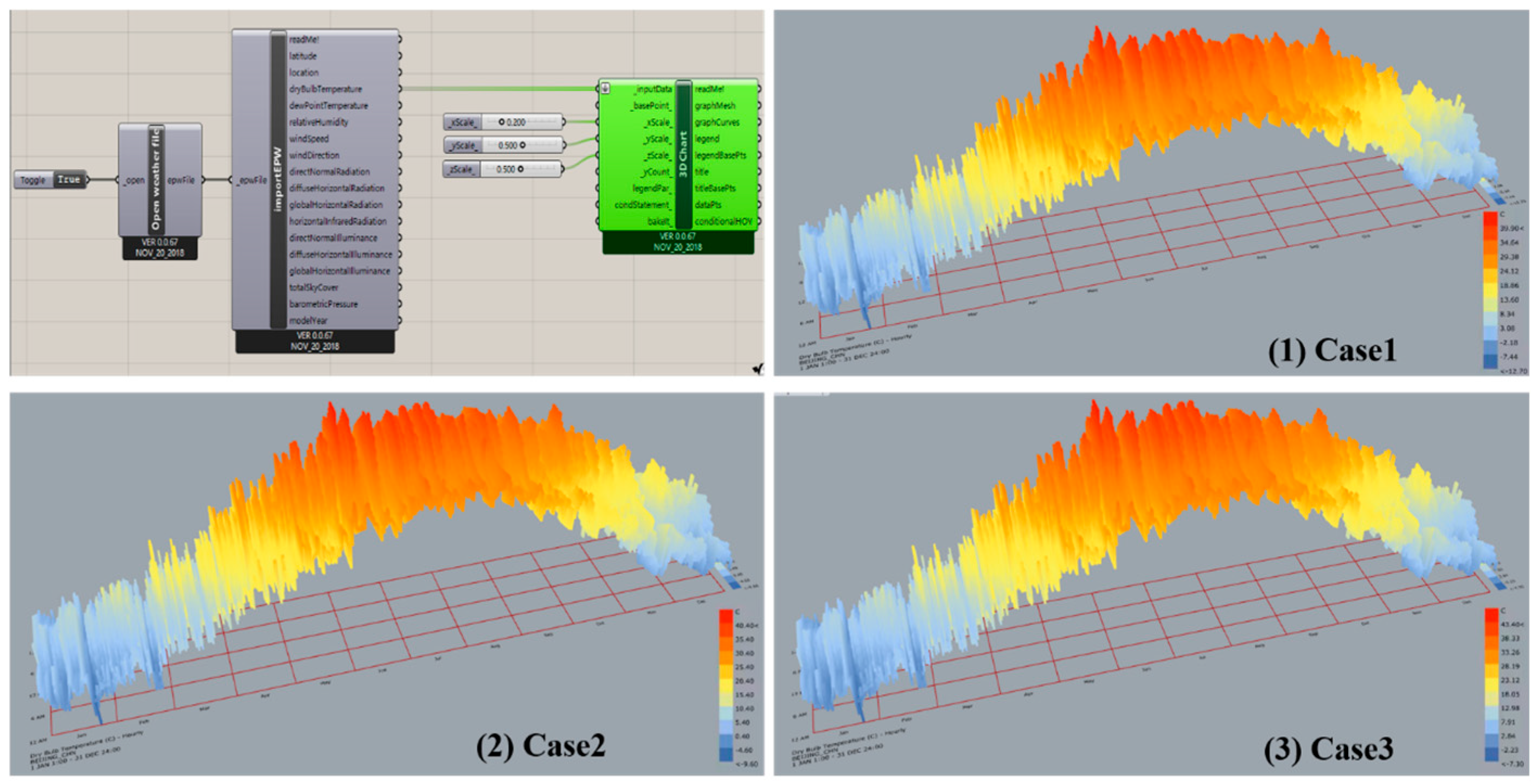
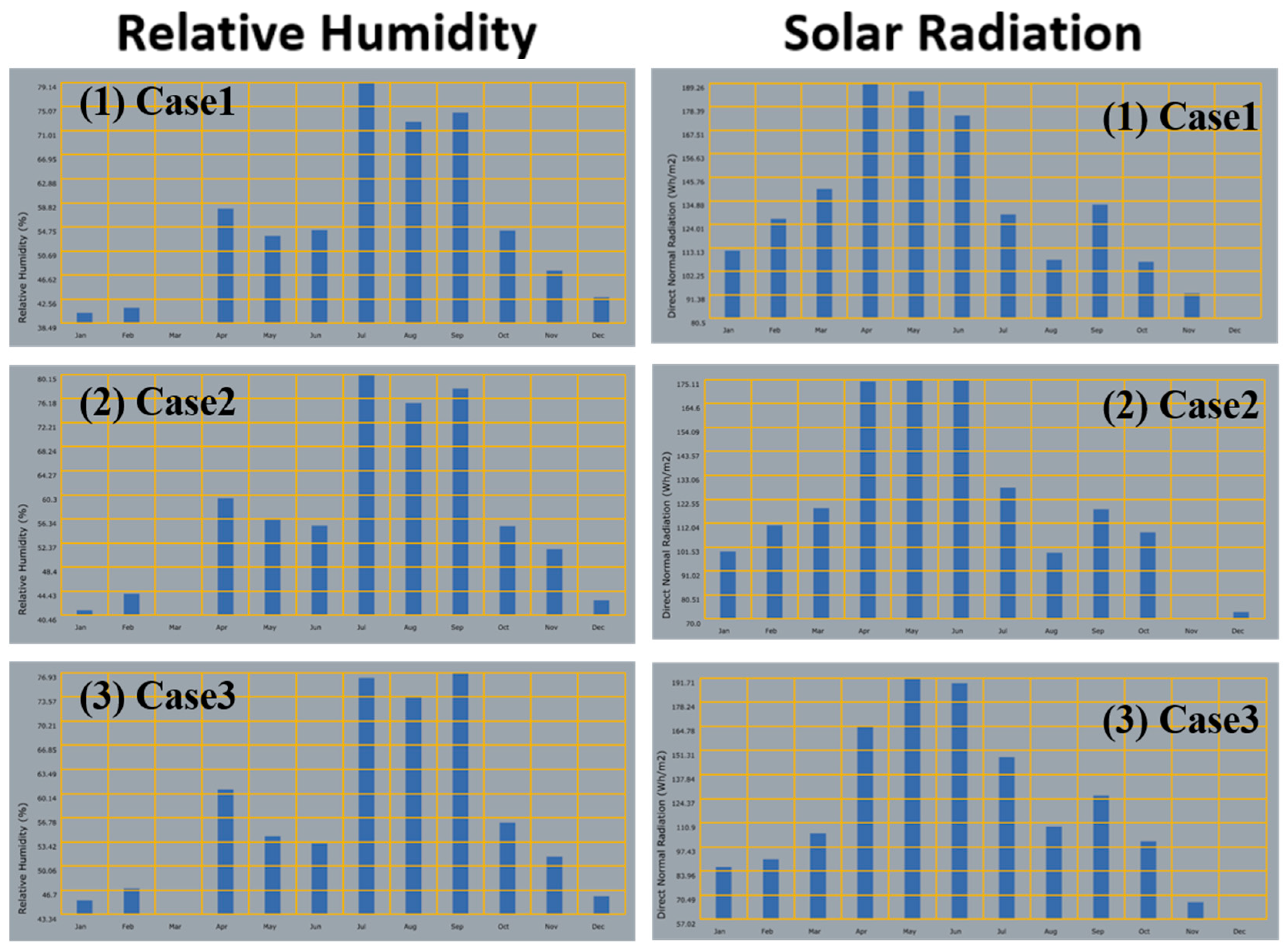
The study establishes three macro climate scenarios: Case 1 represents the current baseline scenario (2020s), while Case 2 and Case 3 correspond to future climate scenarios at the mid-life (2050s) and end-of-life (2080s) stages of the building, respectively. Utilizing hourly meteorological data, annual hourly datasets suitable for building performance simulation were constructed. Visualization analysis of key meteorological parameters under the three scenarios in Tianjin was conducted through the Rhino-Grasshopper-Ladybug platform. Figure 10 demonstrates a persistent upward trend in hourly outdoor dry-bulb temperature under climate change progression. Figure 11 further compares the monthly average relative humidity and direct solar radiation variations, revealing that relative humidity generally exhibits a declining trend, though with monthly variations—showing steady increases during January–April, September, and November–December, while May, June–August, and October display an initial rise followed by decline; direct solar irradiance changes are more complex, with continuous decreases during January–March; overall decline in April; sustained increase in June; initial decline followed by rise in May, July–September and November; and an initial rise followed by decline in October and December. Overall, solar direct irradiance demonstrates more pronounced fluctuations compared to temperature and humidity variations. In summary, as the climate evolves, key meteorological parameters exhibit increasingly diversified and complex changing patterns, with solar radiation conditions showing particularly significant variability.

2.3.2. Uncertainty Analysis Method

This study introduces an uncertainty analysis methodology to evaluate the differential performance of BIPV buildings under baseline and future climate scenarios. By calculating the coefficient of variation (δ), we objectively quantify the uncertainty impacts induced by climate change on BIPV building performance [35]. This approach systematically assesses whether, and to what extent, the actual building performance may deviate from its initial optimal design targets under the dual drivers of climate evolution and technological advancement, thereby providing critical decision support for developing forward-looking and highly adaptive building design solutions.

$$\mathsf{\delta }={\displaystyle \frac{\mathsf{\epsilon }-\mathsf{ϵ}}{\mathsf{ϵ}}}\times 100\%$$

(10)

where $\mathsf{\epsilon }$ and $\mathsf{ϵ}$ represent the BIPV building performance under future climate change scenarios and the baseline scenario, respectively. The building performance specifically refers to GWP (global warming potential), EPV (electricity production volume), FI (flexibility index), and LCC (life cycle cost).

2.4. Stochastic Generation Model for BIPV Building Integrated Performance

2.4.1. Probabilistic Distribution Model of Design Variables

A probabilistic model (also referred to as a statistical model) is a mathematical construct that describes relationships between random variables, typically characterizing mutually non-deterministic probabilistic interactions among one or more stochastic variables. Probability density functions are employed to quantify the likelihood of an uncertain variable approximating its design value. Commonly utilized probability distributions include uniform, triangular, normal, and t-distributions [36]. The selection of probability distributions for passive design variables varies according to research objectives. When evaluating existing building performance, thermophysical parameters of building envelopes may be appropriately modeled using normal distributions. Conversely, during the architectural design phase aimed at identifying effective solutions, uniform distributions are generally recommended [37]. Discrete probability distributions are applied to describe uncertain time-series variables influenced by human behavior, such as window ventilation operations and shading adjustments. This study implements discrete distributions to characterize three distinct types of photovoltaic windows and deterministic occupancy patterns. The quantitative models established for design parameters are systematically presented in

Table 12. Sampling range of input parameters.

	Input Variable Name	Tag	Probability Distribution	Unit	Sampling Boundary
X1	Orientation	@@orientation@@	Uniform	°	[0,180]
X2	Wall Insulation	@@north wall u@@	Uniform	W/(m2K)	[0.15,0.45]
X3		@@sourth wall u@@
X4		@@west wall u@@
X5		@@east wall u@@
X6		@@wall density@@	Uniform	kg/m3	[500,2500]
X7		@@specific heat@@	Uniform	J/(kg K)	[1000,2500]
X8	Surface Heat Absorption Coefficient	@@roof absolute@@	Uniform	/	[0.1,0.9]
X9		@@wall absolute@@		/	[0.1,0.9]
X10	Window-to-Wall Ratio PV1	@@WWR north@@	Uniform	/	[0.2,0.3]
X11		@@WWR south@@			[0.2,0.5]
X12		@@WWR west@@			[0.2,0.35]
X13		@@WWR east@@			[0.2,0.35]
X14	Shading Angle PV2	@@overhang degree@@	Uniform	°	[0,90]
X15	Photovoltaic Window PV3	@@visible transmission@@	Discrete	/	{0.07,0.177;0.327}
X16		@@PV SHGC@@	Discrete	/	{0.129;0.186;0.271}
X17		@@PV generator@@	Discrete	%	{9.91,7.73,6.04}
X18	Window Insulation	@@north window u@@	Uniform	W/(m2K)	[1.32,1.76]
X19		@@south window u@@
X20		@@west window u@@
X21		@@east window u@@
X22		@@SHGC@@	Uniform	/	[0.25,0.55]
X23	Roof Insulation	@@roof u@@	Uniform	W/(m2K)	[0.1,0.25]
X24		@@roof density@@	Uniform	kg/m3	[500,2500]
X25		@@roof specific heat@@	Uniform	J/(kg K)	[800,2000]
X26	Internal Wall Insulation	@@interior furnishings@@	Uniform	W/(m2K)	[0.3,0.5]
X27	Air Change Rate	@@ACH@@	Uniform	1/hr	[0.1,0.6]
X28	Equipment Power Density	@@equipment density@@	Uniform	W/m2	[2,8]
X29	Lighting Power Density	@@lighting density@@	Uniform	W/m2	[3,7]
X30	Occupancy	@@people occupation@@	Discrete	person	{1,2,3,4}

.

2.4.2. Monte Carlo Simulation

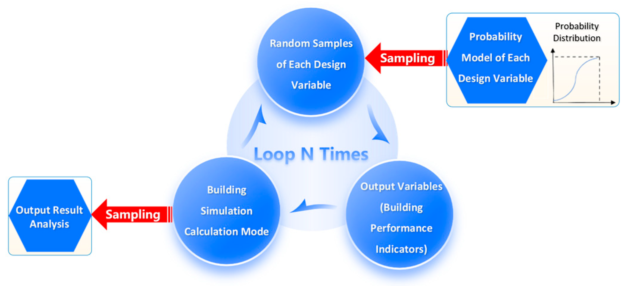
Uncertainty in the architectural design phase arises from limitations in information accessibility and computational tools. To analyze the impact of static uncertain parameters on the comprehensive performance of building-integrated photovoltaics, appropriate uncertainty analysis methods are required. Based on the category of uncertain information being processed, these methods can be classified into interval mathematics, grey theory, fuzzy theory, probabilistic analysis, and rough set theory, with probabilistic analysis being the most widely adopted approach in building design [38]. Probabilistic analysis utilizes the distribution functions of random variables as its foundation, quantifying the uncertainty of input parameters with known distributions or distributions inferred from available information. The quantification results manifest as probability distributions of output variables [38]. In this study, probabilistic analysis is employed to establish relationships between stochastic building performance samples generated from uncertain static design parameters. The Monte Carlo method, also referred to as stochastic simulation, represents a general numerical approach grounded in probability and statistical theory. The specific procedural workflow is illustrated in Figure 12.

To ensure the reliability of uncertainty quantification results, Monte Carlo simulations typically require a sufficiently large number of sampling iterations. Simple random sampling often necessitates an increased sample size due to the clustering tendency of sampled points, consequently escalating computational demands and prolonging processing duration. The implementation of Latin Hypercube Sampling effectively mitigates these limitations by providing improved stratification with reduced sample requirements.

2.5. Sensitivity Analysis Method

2.5.1. Correlation Analysis Method

Prior to conducting global sensitivity analysis (GSA), this study performed preliminary correlation analysis using SPSS Statistics (version 29.0) to identify potential association patterns between input variables and output responses. This preliminary assessment aims to reveal potential linear or nonlinear relationships among variables, thereby informing the selection of appropriate global sensitivity analysis methodologies. Commonly employed correlation analysis techniques in SPSS include the chi-square test, Spearman’s rank correlation coefficient, and Pearson correlation coefficient [39].

For correlation analysis between two continuous variables, the most commonly used metric is the Pearson correlation coefficient, which is in the range of [−1, 1]. Values closer to |1| indicate stronger linear relationships between variables [40]. Pearson correlation analysis is a parametric method that requires variables to exhibit linear correlation trends and approximately follow a bivariate normal distribution. However, this method is sensitive to outliers, as extreme values may significantly distort analytical results. In contrast, Spearman’s rank correlation coefficient does not depend on the specific distributional form of the original variables, offering broader applicability as a nonparametric statistical approach, though generally with lower statistical power compared to the Pearson method.

Considering the data characteristics and analytical objectives of this study, the Pearson correlation coefficient was selected for preliminary assessment of inter-parameter correlations. This analysis was conducted separately on datasets generated through both Latin Hypercube Sampling (LHS) and random sampling strategies, enabling systematic examination of variable correlation structure consistency across different sampling methodologies and establishing a foundation for subsequent sensitivity analysis.

2.5.2. Global Sensitivity Analysis Method

Global sensitivity analysis serves as a critical methodology for identifying key input parameters in complex models and quantifying their contribution to output uncertainty. The primary approaches can be categorized into four groups: variance-based methods, metamodeling techniques, screening methods, and regression-based analyses [41]. In this study, to comprehensively and accurately assess parameter sensitivity within the building energy model, we systematically compared the characteristics of different methodologies and ultimately selected the variance-based approach as the core analytical framework.

Among various methodologies, variance-based approaches (such as FAST and Sobol methods) demonstrate distinctive advantages due to their model-free nature, requiring no presumptive functional forms and thus being particularly suitable for highly nonlinear, non-additive complex systems. Specifically, the classical FAST method efficiently computes main effects of parameters but exhibits limitations in capturing interaction effects among variables [41]. In contrast, the Sobol method employs sophisticated variance decomposition techniques to comprehensively separate both main effects and interaction effects of parameters, thereby providing a more complete sensitivity profile [41]. Whereas regression-based methods (utilizing coefficients such as SRC and PCC), despite their computational efficiency and widespread application in building energy analysis, typically rely on assumptions of linearity or monotonicity, consequently limiting the completeness of analytical results when addressing complex nonlinear responses [41].

Based on these considerations, the Sobol method was selected as the core analytical framework due to its theoretical completeness in addressing nonlinear and interaction effects, demonstrating superior suitability for the complex system analysis scenario in this study. The implementation of this method builds upon variance decomposition principles, enabling precise quantification of each input parameter’s contribution (including interaction effects) to the total output variance, thereby facilitating quantitative identification and systematic sensitivity ranking of key parameters. Through this approach, a number of sensitivity indices ranging from 0 to 1 are computed, where higher values indicate stronger parameter influence on model outputs. These indices are systematically classified according to the threshold ranges established in

Table 13. Value range of correlation coefficients [42]. Reproduced with permission from Dongdong Ge, Zhendong Zhang, Xiangdong Kong, and Zhiping Wan, from Applied Sciences, published by MDPI, 2022.

Absolute Value of Correlation Coefficient	Correlation Strength
0.8~1.0	Very Strong Correlation
0.6~0.8	Strong Correlation
0.4~0.6	Moderately Strong Correlation
0.2~0.4	Weak Correlation
0.0~0.2	Very Weak or No Correlation

, allowing efficient identification of the most influential variables driving output uncertainty.

Finally, it should be noted that all computational tasks in this study were performed on a desktop workstation equipped with an Intel Core i7-10700K CPU @ 3.80 GHz, 32 GB RAM, and 1 TB SSD storage. The operating system used was Windows 11 64-bit Professional Edition. The Monte Carlo simulation was configured with 1000 sampling iterations, with each complete BIPV building performance simulation (including energy consumption, power generation, carbon emissions, and economic calculations) taking approximately 45 s on average, resulting in a total computation time of about 12.5 h. The Sobol sensitivity analysis was conducted based on the Monte Carlo sampling results, requiring an additional computation time of approximately 2 h. All computational tasks were executed using single-core serial processing to ensure consistency and reproducibility of the results.

3. Results

3.1. Results of Input Parameter Correlation Analysis

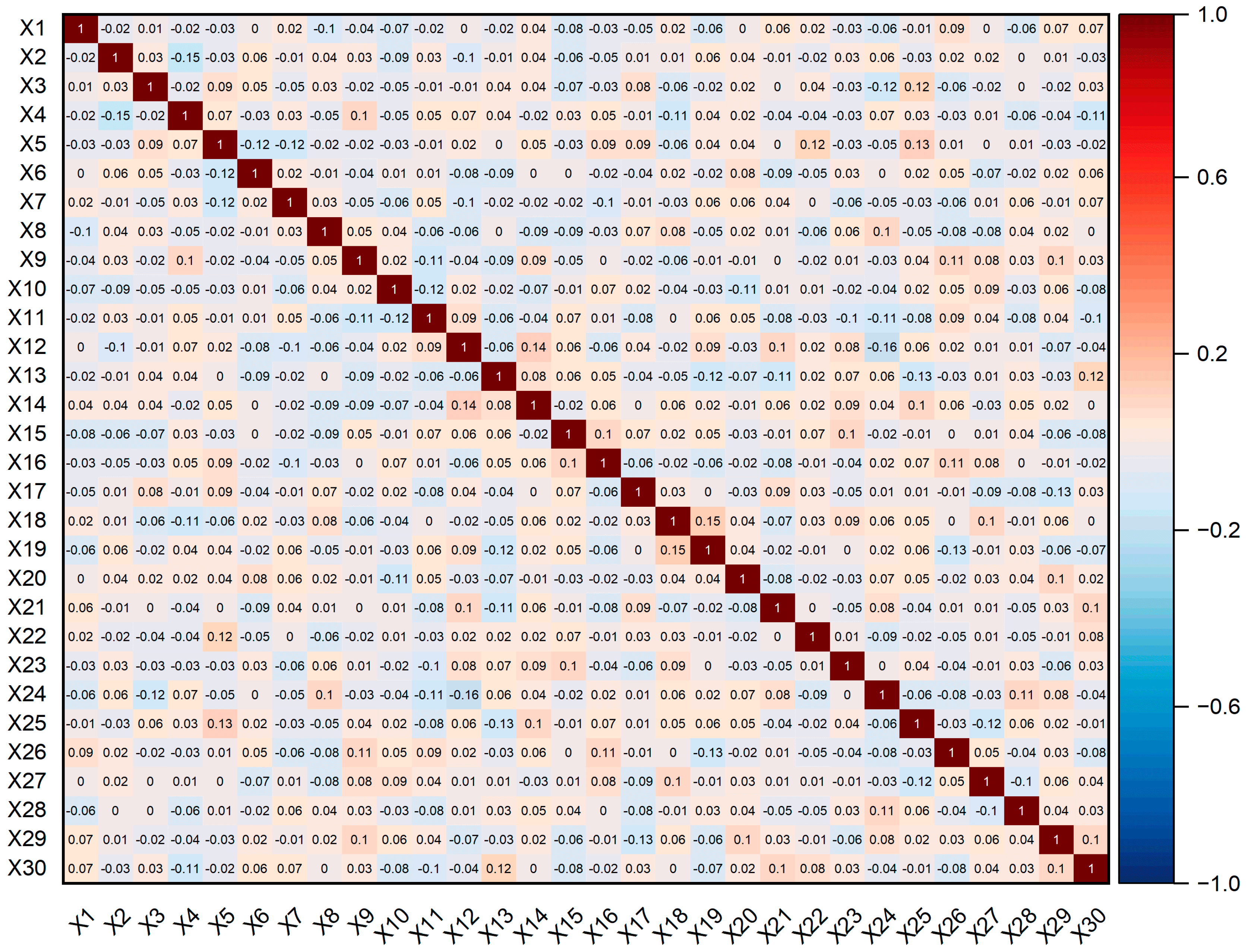
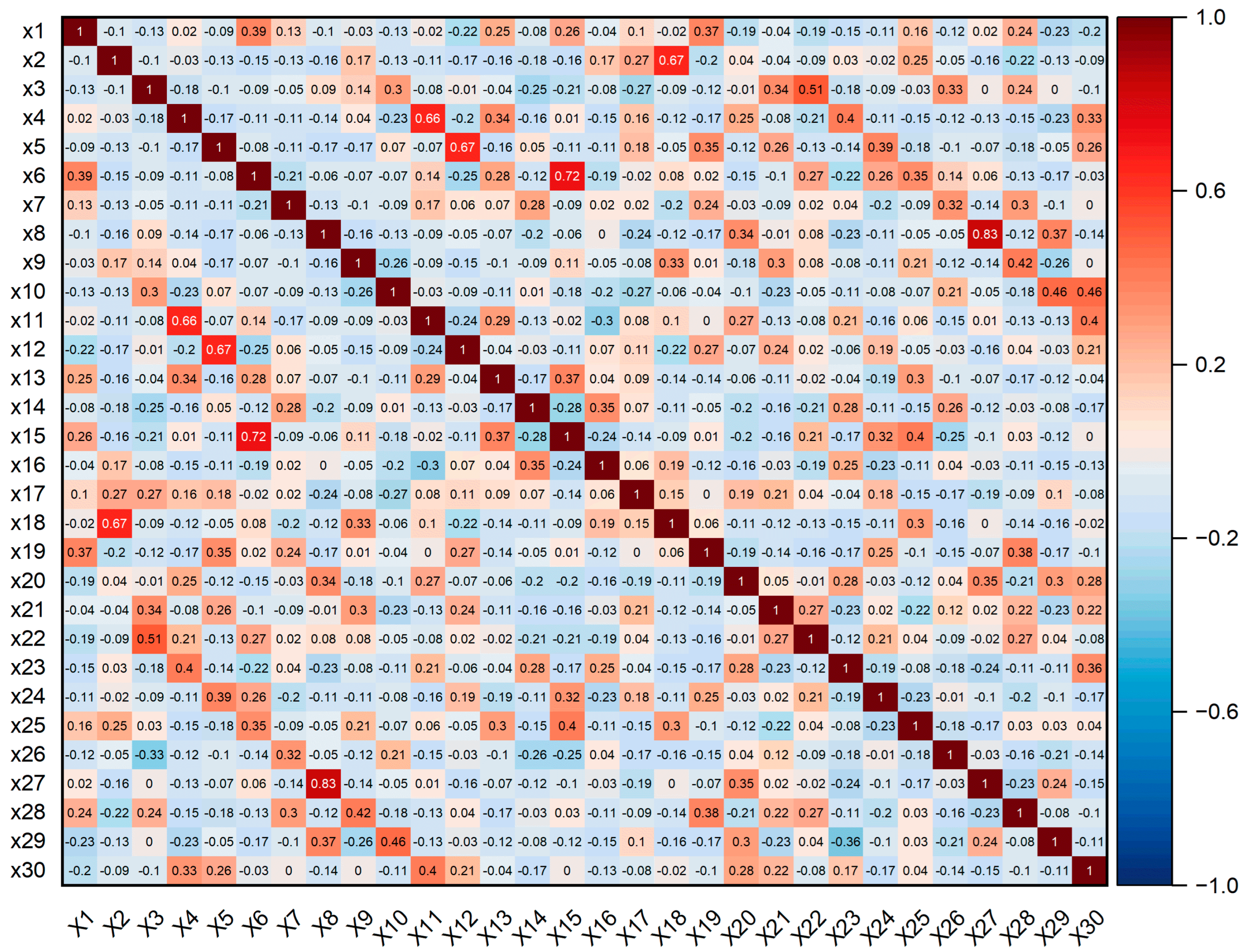
Figure 13 and Figure 14 present the correlation analysis results among input variables under Latin Hypercube Sampling (LHS) and random sampling conditions, respectively. Comprehensive analysis demonstrates that LHS significantly outperforms random sampling in controlling inter-variable correlations, rendering it more suitable for subsequent global sensitivity analysis.

Specifically, under Latin Hypercube Sampling (LHS) conditions (Figure 13), the Pearson correlation coefficients between input variables predominantly range from −0.17 to 0.15, with all absolute coefficient values remaining below 0.2. These results indicate only negligible correlations among variables, essentially satisfying the independence assumption required for global sensitivity analysis. In contrast, under random sampling conditions (Figure 14), the correlation coefficients demonstrate a wider distribution, primarily spanning −0.2 to 0.4, with several notably elevated coefficients observed. These substantial correlations reveal that random sampling fails to effectively control inter-variable dependencies, and its inherent correlation structure may potentially interfere with subsequent sensitivity analysis, even leading to misinterpretation of parameter influences.

In summary, Latin Hypercube Sampling (LHS) effectively suppresses spurious correlations introduced by the sampling process, ensuring fundamental independence among variables and thereby establishing a more reliable data foundation for sensitivity analysis. Consequently, subsequent analyses in this study will primarily utilize LHS-generated data to ensure the robustness and reliability of conclusions.

In summary, this study employs Latin Hypercube Sampling (LHS) to control inter-variable correlations, a method selected based on its established authority in the field of uncertainty analysis. The seminal work of McKay et al. [43] clearly indicates that LHS outperforms simple random sampling in terms of covering the input variable space and ensuring the statistical properties of outputs. The computational results of this study (Figure 13 and Figure 14) validate the effectiveness of this method in the current context, as it effectively suppresses spurious correlations introduced by the sampling process, ensures fundamental independence among variables, and provides a more reliable data foundation for sensitivity analysis. Therefore, all subsequent analyses are based on LHS-sampled data to ensure the robustness and reliability of the research conclusions.

3.2. Parameter Sensitivity Analysis Results

Based on the Sobol sensitivity analysis method, first-order sensitivity indices measure the independent contribution of individual input variables to the variance of the output, reflecting their isolated impact on the model output. In contrast, total-order indices comprehensively account for the interactions between the variable and others, capturing its overall influence on the system output under coupled conditions. This study systematically presents the specific numerical results of the first-order and total-order indices for each variable in Appendix A.2 and Appendix A.3, respectively. Preliminary analysis reveals non-negligible interactions among the input variables, which cannot be fully captured by first-order indices alone. Relying solely on first-order indices may lead to an underestimation of variable influence. Therefore, this study primarily uses the total-order sensitivity index as the basis for determining variable significance. Regarding the determination of the significance threshold for total-order indices, traditional approaches often rely on subjective experience or predefined fixed criteria. To enhance objectivity, this study adopts the arithmetic mean of the absolute values of all variables’ total-order indices as the discrimination threshold. Variables exceeding this threshold are considered to have a significant impact on the output, while those below are deemed non-significant.

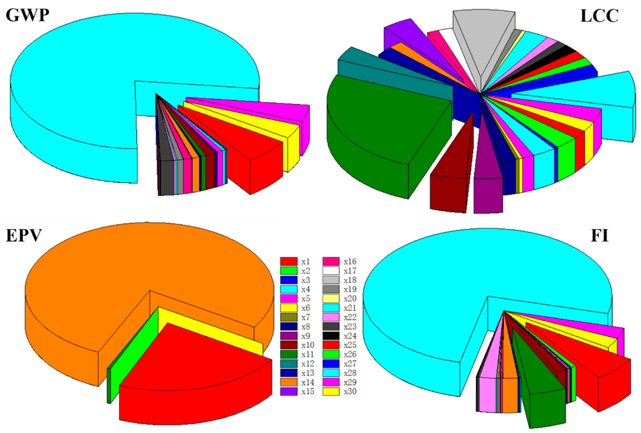
Based on the total-order sensitivity index contribution pie chart presented in Figure 15, the following variables are identified as exerting significant influence on the comprehensive performance of building-integrated photovoltaics (including energy consumption, indoor comfort, and power generation benefits): X1 (building orientation), X9 (wall thermal absorptance), X10 (north window-to-wall ratio), X11 (south window-to-wall ratio), X12 (west window-to-wall ratio), X14 (photovoltaic shading angle), X15 (photovoltaic window visible transmittance), X18 (north window insulation level), X28 (equipment power density), X29 (lighting power density), and X30 (occupancy density). These parameters collectively demonstrate critical impacts on system behavior through complex intervariable interactions. In summary, employing Sobol total-order sensitivity analysis, this study not only identifies key parameters with predominant influence on building integrated performance under multivariate interaction scenarios, but also reveals potential mechanisms of synergistic or antagonistic effects among variables. These analytical outcomes provide crucial foundations for subsequent BIPV performance optimization, parameter adjustment strategies, and uncertainty management, thereby facilitating more precise resource allocation and system control during both design and operational phases.

Comparing the aforementioned sensitivity analysis results with existing studies reveals both shared patterns and distinct characteristics. Consistent with our finding that photovoltaic shading angle is a key parameter, Sadatifar et al. [12] also identified it as one of the core variables for achieving the synergistic optimization of “power generation-energy saving-comfort” in their multi-objective research, which validates the effectiveness of our model in identifying such critical design parameters. However, whereas Chen et al. [11] focused more on reducing carbon emissions through building form and envelope optimization, and Sadatifar et al. [12] concentrated on balancing power generation, energy efficiency, and comfort, this study introduces an energy flexibility index to further reveal the significant impact of equipment and lighting power density on this emerging metric. This finding addresses the limitations of traditional analytical frameworks that primarily focus on building performance itself, providing more specific parametric guidance for grid-interactive BIPV building design.

3.3. Uncertain Impacts of Climate Change on BIPV Building Performance

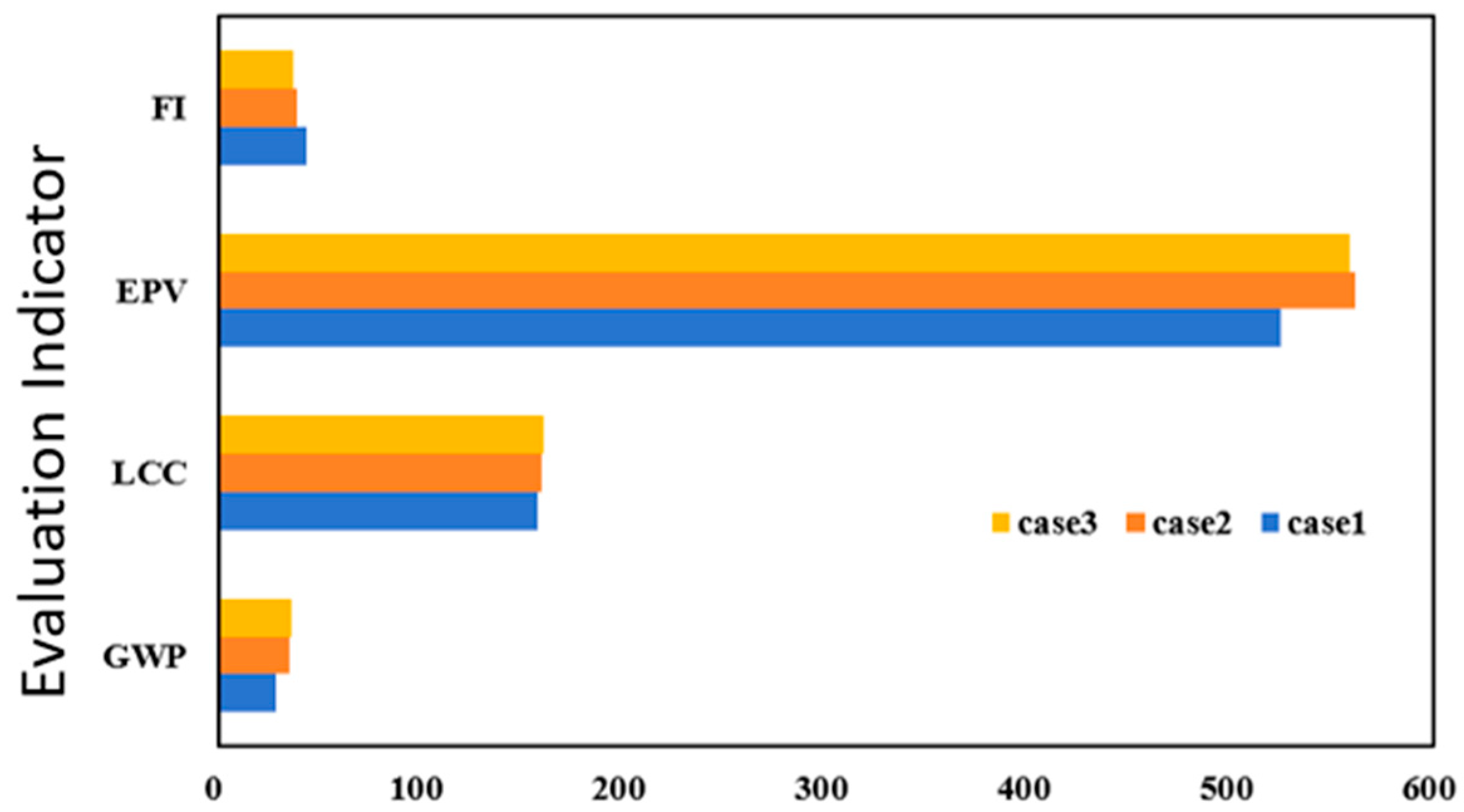
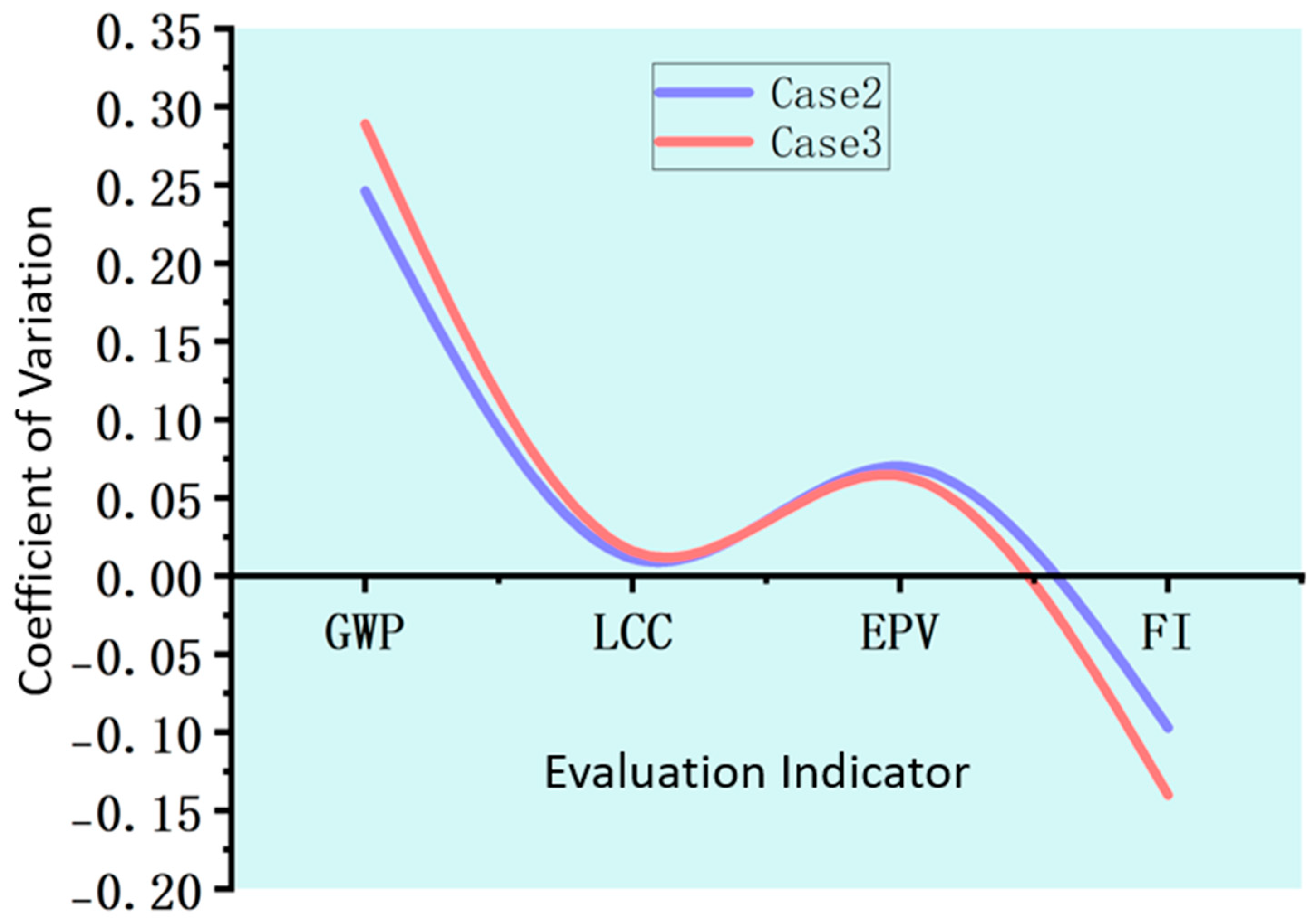
Through performance simulations of BIPV buildings under Case 1 (baseline scenario), Case 2 (2050s climate scenario), and Case 3 (2080s climate scenario), this study reveals the evolving trends of building performance under different future climate scenarios, considering global climate change impacts, as illustrated in Figure 16. The results demonstrate that with intensifying climate change, both carbon emissions and life cycle costs of BIPV buildings show increasing trends, while energy flexibility gradually declines, indicating persistent challenges to overall building performance in the future. However, regarding power generation performance, due to variations in direct solar radiation conditions, BIPV buildings exhibit the highest generation potential during the mid-building life cycle (Case 2), suggesting possible enhancements in photovoltaic conversion efficiency during specific climate phases.

This study reveals the evolving patterns of BIPV performance under climate change, which aligns with existing research while highlighting the advantages of our methodology in long-term risk assessment. Similar to our finding that BIPV power generation potential increases under mid-term climate conditions due to changes in solar radiation, Tang et al. [18] also emphasized the decisive influence of solar radiation conditions on the power generation potential of BIPV at the urban scale. However, many studies aimed at optimizing BIPV system performance, such as Xu et al.’s [19] parametric analysis of high-rise residential buildings in Hong Kong, typically base their evaluations on static or historical climate conditions. While such studies can effectively assess system performance during specific periods, they fail to capture long-term climate evolution trends driven by global warming and the associated risks of extreme events. Wang et al.’s [21] research on the increasing frequency of extreme windless and low-sunlight events and their impact on rising electricity costs directly warns of the systemic risks posed by ignoring year-to-year climate variations. In contrast, by incorporating future climate scenarios and an uncertainty analysis framework, this study quantifies the potential deviations in performance indicators over the long term, providing a more forward-looking perspective for evaluating the robustness and climate adaptability of BIPV systems throughout their life cycle.

Collectively, although climate change adversely affects building energy consumption, carbon emissions, and economic performance, photovoltaic technology demonstrates potential for more efficient energy harvesting under certain future climate conditions. Therefore, actively advancing photovoltaic technology applications and promoting widespread BIPV implementation will represent crucial development pathways for addressing climate challenges and facilitating building decarbonization transitions.

Figure 17 and

Table 14. Robustness evaluation indicators for different future scenarios considering climate change [31]. Reproduced with permission from Shilei Lu, Hongcheng Zhu, Quanyi Lin, Yongjun Sun, Shengying Huang, and Ran Wang, from Journal of Building Engineering, published by Elsevier, 2025.

$\mathsf{\delta }$	GWP	LCC	EPV	FI
Case 2	0.246	0.011	0.070	−0.097
Case 3	0.289	0.016	0.064	−0.140

present robustness evaluation indicators for different future scenarios considering climate change. The results indicate that the building sector in future high-renewable energy power systems will face significant climate adaptation challenges. Key metrics, including carbon emission intensity and energy flexibility, exhibit substantial fluctuations across different climate pathways, reflecting their high sensitivity and exposure to climate change. These findings further reveal the particularly pronounced impact of climate constraints on the carbon footprint during building operational phases.

To address these challenges, the following pathways should be actively promoted. At the technical level, climate-responsive design strategies should be integrated, including enhanced thermal inertia of building envelopes, adoption of adjustable shading and natural ventilation systems, and development of integrated photovoltaic–storage–direct current–flexibility (PSDF) energy systems. At the policy level, building carbon accounting methodologies and low-carbon performance incentive mechanisms should be refined to shift the focus from “energy consumption control” to “carbon emission management.” At the system coordination level, leveraging smart grid technologies and demand-side response mechanisms should expand buildings’ potential as flexible loads, transforming them from mere energy consumers into proactive “prosumers.”

In conclusion, climate adaptation must be deeply integrated throughout the entire building design and operational life cycle. Through systematic innovation in technology, policy, and mechanisms, the climate resilience of the building sector can be effectively enhanced, achieving synergistic advancement of green low-carbon transition and systemic security.

3.4. Life Cycle Economic and Reliability Analysis

Based on the aforementioned life cycle cost (LCC) model and cost parameter analysis, the impact of climate change on the economic sustainability of BIPV buildings cannot be overlooked. Simulation results (see Figure 17) indicate that as climate change intensifies, the life cycle cost of BIPV buildings shows a significant upward trend: Case 2 (2050s) increases by 1.1% compared to the baseline scenario, while Case 3 (2080s) rises further to 1.6%. This cost escalation primarily stems from three factors: increased cooling energy costs due to prolonged air conditioning operation caused by rising temperatures, higher maintenance costs resulting from accelerated equipment aging due to frequent extreme weather events, and efficiency degradation caused by the accelerated performance decline of photovoltaic materials in high-temperature environments.

The long-term maintenance and reliability of BIPV systems are crucial to ensuring their economic sustainability. According to the operational and maintenance cost data in Table 11, the annual maintenance cost of the photovoltaic system is 21,898 ¥, and the inverter replacement cost is 3120.5 ¥ per year. In the context of climate change, these costs may increase significantly. Extreme high temperatures can accelerate the aging of component materials, frequent extreme weather events may raise the risk of physical damage, and temperature fluctuations can affect the stability of electronic equipment—all of which pose challenges to the long-term reliability of the system. Therefore, it is necessary to establish a preventive maintenance system and select equipment with stronger climate adaptability to enhance system reliability.

Beyond techno-economic factors, the widespread adoption of BIPV technology faces multiple challenges in architectural design and regulatory constraints. From an architectural design perspective, integrating photovoltaic facades, shading systems, and windows requires balancing aesthetics, structural safety, and energy efficiency. Building codes impose technical requirements for fire prevention, waterproofing, and structural strength, which limit the design flexibility of BIPV systems. On the policy and regulatory front, although the national government has set a target for photovoltaic coverage in new buildings by 2025, local implementation rules and standards remain underdeveloped. This is particularly evident in the lack of unified technical standards and approval guidelines for BIPV retrofitting in existing buildings. Furthermore, ambiguities in grid connection policies—such as technical requirements for integration, feed-in tariff subsidies, and electricity trading mechanisms—increase policy-related investment risks for projects.

Finally, from a broader environmental sustainability perspective, while this study primarily focuses on carbon emissions during the operational phase, a comprehensive assessment of BIPV’s environmental benefits requires consideration of its cumulative environmental impacts throughout the entire life cycle. The manufacturing process of photovoltaic components involves high energy consumption and certain carbon emissions. Although power generation during the operational phase can offset these emissions, it takes a longer time to achieve true carbon neutrality. Additionally, the rare metals and toxic substances contained in the components may cause pollution during disposal, necessitating the establishment of a robust recycling system. Future research should develop more comprehensive life cycle assessment models for BIPV to provide a scientific basis for technology selection and policy formulation.

4. Conclusions

Building-integrated photovoltaics (BIPVs), as a pivotal technology for enhancing renewable energy utilization in buildings, currently face challenges, including the lack of integrated design models, unidimensional performance analysis, and insufficient consideration of climate change factors. To address these limitations, this study proposes a comprehensive performance analysis methodology for BIPV systems that incorporates global climate change impacts. The methodology is developed through four key components: (1) establishing an integrated BIPV simulation model for photovoltaic curtain walls, shading systems, and roofs by coupling EnergyPlus, Optics6, and WINDOW 7.7; (2) constructing a comprehensive performance evaluation framework encompassing four dimensions: global warming potential (GWP) of carbon emissions, electricity generation, energy flexibility, and economic costs; (3) generating hourly meteorological data under future climate scenarios, covering both mid-term (2050s) and long-term (2080s) building life cycle stages using the CCWorldWeatherGen tool; and (4) implementing Monte Carlo simulations to generate comprehensive BIPV performance datasets across variable combinations, followed by sensitivity and uncertainty analyses to identify key influencing factors and quantify climate change impacts on various performance indicators. The main conclusions are summarized as follows:

• The sensitivity analysis of design parameters reveals that variables exerting significant influence on the comprehensive performance of building-integrated photovoltaics (including energy consumption, indoor comfort, and power generation benefits) include: building orientation, wall thermal absorptance, north window-to-wall ratio, south window-to-wall ratio, west window-to-wall ratio, photovoltaic shading angle, photovoltaic window visible transmittance, north window insulation level, equipment power density, lighting power density, and occupancy density. Specifically, equipment power density and lighting power density demonstrate the most pronounced combined effects on carbon emissions and flexibility index. Variations in building envelope thermal performance exhibit greater impact on life cycle costs than on carbon emissions. Photovoltaic shading shows more responsive power generation performance compared to photovoltaic curtain walls and windows. Furthermore, the east wall insulation level, photovoltaic window visible transmittance, and solar heat gain coefficient present non-negligible influences on building economic costs.
• The uncertainty analysis of climate change impacts demonstrates that with intensifying climate change, both carbon emissions and life cycle costs progressively increase while energy flexibility continuously declines, indicating sustained pressure on overall system performance. However, under specific mid-term climate conditions, BIPV systems exhibit enhanced power generation potential due to altered solar radiation patterns, suggesting possible improvements in photovoltaic energy conversion efficiency in future scenarios. To address climate challenges, it is imperative to integrate climate-adaptive design strategies with advanced energy systems such as integrated photovoltaics–storage-direct current–flexibility (PSDF) configurations, while simultaneously promoting policy mechanism transformations. Consequently, actively advancing BIPV technology implementation and embedding climate resilience throughout the building life cycle represent crucial pathways for achieving building decarbonization and enhancing systemic climate adaptation capacity.

The study has limitations: its methodology relies on static assumptions and struggles to capture real-world dynamics, while its data and case studies are context-specific, limiting the generalizability of the findings. Future work should integrate dynamic simulations and diverse data to validate the framework, alongside exploring the integration of smart technologies to enhance the adaptability of BIPV design.

References

1. Anjum, T.; Alam, M.M.; Hossain, I.; Gomaa, M.; Kumar, L. Methods, technologies and challenges of building integrated photovoltaic thermal (BIPV/T) systems to achieve net-zero in high rise buildings: A systematic review. J. Build. Eng. 2025, 114, 114284. [Google Scholar] [CrossRef]
2. Assoa, Y.B.; Thony, P.; Messaoudi, P.; Schmitt, E.; Bizzini, O.; Gelibert, S.; Therme, D.; Rudy, J.; Chabuel, F. Study of a building integrated bifacial photovoltaic facade. Sol. Energy 2021, 227, 497–515. [Google Scholar] [CrossRef]
3. Liu, L.X.; Zhang, X.Y.; Cheng, Q. Optimization design of a new polyhedral photovoltaic curtain wall for different climates in China. Sustain. Energy Technol. 2024, 72, 104078. [Google Scholar] [CrossRef]
4. Huang, S.F.; Wang, M.; Zou, B.; Wang, S.H.; Xiong, Y.; Fu, G.H.; Sun, Q.H.; Dou, S.; Peng, J.Q. Structural optimization of CdTe photovoltaic window based on climate adaptability. Energy Build. 2025, 343, 115926. [Google Scholar] [CrossRef]
5. Li, J.Y.; Wu, J.M.; Xu, H.P. Impact of photovoltaic energy-saving window on building heating load. J. Build. Eng. 2025, 108, 112853. [Google Scholar] [CrossRef]
6. Li, X.; Peng, J.Q.; Li, N.P.; Wu, Y.P.; Fang, Y.P.; Li, T.; Wang, M.; Wang, C.L. Optimal design of photovoltaic shading systems for multi-story buildings. J. Clean. Prod. 2019, 220, 1024–1038. [Google Scholar] [CrossRef]
7. Ye, Y.X.; Zhu, R.; Yan, J.Y.; Lu, L.; Wong, M.S.; Luo, W.; Chen, M.; Zhang, F.; You, L.L.; Wang, Y.F.; et al. Planning the installation of building-integrated photovoltaic shading devices: A GIS-based spatiotemporal analysis and optimization approach. Renew. Energy 2023, 216, 119084. [Google Scholar] [CrossRef]
8. El-Nagar, D.H.; Emam, M.; El-Betar, A.A.; Nada, S.A. Combining active and passive cooling techniques for maximizing power generation and thermal utilization of photovoltaic panels. Renew. Energy 2025, 250, 123310. [Google Scholar] [CrossRef]
9. Benaddi, F.Z.; Boukhattem, L.; Tabares-Velasco, P.C. Multi-objective optimization of building envelope components based on economic, environmental, and thermal comfort criteria. Energy Build. 2024, 309, 113909. [Google Scholar] [CrossRef]
10. Wijeratne, W.M.P.U.; Samarasinghalage, T.I.; Yang, R.J.; Wakefield, R. Multi-objective optimisation for building integrated photovoltaics (BIPV) roof projects in early design phase. Appl. Energy 2022, 309, 118479. [Google Scholar] [CrossRef]
11. Chen, Z.S.; Cui, Y.Q.; Cai, H.B.; Zheng, H.C.; Ning, Q.; Ding, X. Multi-objective optimization of photovoltaic facades in prefabricated academic buildings using transfer learning and genetic algorithms. Energy 2025, 328, 136470. [Google Scholar] [CrossRef]
12. Sadatifar, S.; Johlin, E. Multi-objective optimization of building integrated photovoltaic solar shades. Sol. Energy 2022, 242, 191–200. [Google Scholar] [CrossRef]
13. Bakmohammadi, P.; Narjabadifam, N.; Jamshidi, M.; Guel, M. A holistic framework to optimize embedding PV systems into building façades. Appl. Energy 2025, 382, 125288. [Google Scholar] [CrossRef]
14. Cai, S.H.; Gou, Z.H. Defining the energy role of buildings as flexumers: A review of definitions, technologies, and applications. Energy Build. 2024, 303, 113821. [Google Scholar] [CrossRef]
15. Hassan, A.A.; El-Rayes, K. Optimal use of renewable energy technologies during building schematic design phase. Appl. Energy 2024, 353, 122006. [Google Scholar] [CrossRef]
16. Jhumka, H.; Yang, S.L.; Gorse, C.; Wilkinson, S.; Yang, R.; He, B.J.; Prasad, D.; Fiorito, F. Assessing heat transfer characteristics of building envelope deployed BIPV and resultant building energy consumption in a tropical climate. Energy Build. 2023, 298, 113540. [Google Scholar] [CrossRef]
17. Wang, M.; Zhao, X.; Li, S.H.; Yang, Z.R.; Liu, K.K.; Wen, Z.H.; Li, Y.H.; Peng, J.Q. Analysis of energy performance and load matching characteristics of various building integrated photovoltaic (BIPV) systems in office building. J. Build. Eng. 2024, 96, 110313. [Google Scholar] [CrossRef]
18. Tang, H.D.; Chai, X.K.; Chen, J.Y.; Wan, Y.; Wang, Y.Q.; Wan, W.; Li, C.Y. Assessment of BIPV power generation potential at the city scale based on local climate zones: Combining physical simulation, machine learning and 3D building models. Renew. Energy 2025, 244, 122688. [Google Scholar] [CrossRef]
19. Xu, K.Y.; Song, S.H.; Xiang, C.Y. Parametric design for combined solar facades for high-rise residential buildings. Sustain. Energy Technol. 2025, 74, 104167. [Google Scholar] [CrossRef]
20. Zou, W.W.; Wang, Y.; Tian, E.Z.; Wei, J.Z.; Peng, J.Q.; Mo, J.H. A New Dynamic and Vertical Photovoltaic Integrated Building Envelope for High-Rise Glaze-Facade Buildings. Engineering 2024, 39, 194–203. [Google Scholar] [CrossRef]
21. Wang, L.C.; Liu, Y.W.; Zhao, L.; Lu, X.; Huang, L.D.; Jin, Y.N.; Davis, S.J.; Aghakouchak, A.; Huang, X.; Zhu, T.; et al. Unraveling climate change-induced compound low-solar-low-wind extremes in China. Natl. Sci. Rev. 2025, 12, nwae424. [Google Scholar] [CrossRef]
22. Gomes, R.; Ferreira, A.; Azevedo, L.; Neto, R.C.; Aelenei, L.; Silva, C. Retrofit measures evaluation considering thermal comfort using building energy simulation: Two Lisbon households. Adv. Build. Energy Res. 2021, 15, 291–314. [Google Scholar] [CrossRef]
23. Chen, X.P.; Cai, Y.X.; Xiao, X.B.; Zheng, Y.Z.; Yang, A.Q. Solar Energy Compensation for Building Energy Saving with Thermal Comfort in a Cold Climate. Electronics 2022, 11, 491. [Google Scholar] [CrossRef]
24. Gasparella, A.; Crawley, D.B.; Pernigotto, G.; Prada, A.; Lawrie, L.K. Extreme weather data in building performance simulation. Build. Simul. Conf. Pr. 2022, 17, 894–901. [Google Scholar] [CrossRef]
25. Wang, R.; Lu, S.L.; Feng, W. Impact of adjustment strategies on building design process in different climates oriented by multiple performance. Appl. Energy 2020, 266, 114822. [Google Scholar] [CrossRef]
26. Deru, M.; Field, K.; Studer, D.; Benne, K.; Griffith, B.; Torcellini, P.; Liu, B.; Halverson, M.; Winiarski, D.; Rosenberg, M.; et al. U.S. Department of Energy Commercial Reference Building Models of the National Building Stock; National Renewable Energy Laboratory: Colorado, CO, USA, 2011.
27. Curcija, C.; Vidanovic, S.; Hart, R.; Jonsson, J.; Powles, R.; Mitchell, R. WINDOW Technical Documentation; Lawrence Berkeley National Laboratory: Berkeley, CA, USA, 2018.
28. Laboratory, L.B.N. Optics Downloads. Available online: https://windows.lbl.gov/optics-downloads (accessed on 23 October 2025).
29. Blair, N.; Dobos, A.P.; Freeman, J.; Neises, T.; Wagner, M.; Ferguson, T.; Gilman, P.; Janzou, S. System Advisor Model, SAM 2014.1.14: General Description; National Renewable Energy Laboratory: Colorado, CO, USA, 2014.
30. SolarWorld. Sunmodule SW 250 Poly/Version 2.0 and 2.5 Frame; SolarWorld: Bonn, Germany, 2012. [Google Scholar]
31. Lu, S.L.; Zhu, H.C.; Lin, Q.Y.; Sun, Y.J.; Huang, S.Y.; Wang, R. Coupling RDA-RPR-NSGAII optimization design method for comprehensive performance of Building Integrated Photovoltaics. J. Build. Eng. 2025, 101, 111869. [Google Scholar] [CrossRef]
32. Barman, S.; Chowdhury, A.; Mathur, S.; Mathur, J. Assessment of the efficiency of window integrated CdTe based semi-transparent photovoltaic module. Sustain. Cities Soc. 2018, 37, 250–262. [Google Scholar] [CrossRef]
33. Jentsch, M.F.; James, P.A.B.; Bahaj, A.S. CCWorldWeatherGen Software: Manual for CCWorldWeatherGen Climate Change World Weather File Generator; University of Southampton: Southampton, UK, 2012. [Google Scholar]
34. Wang, R.; Lu, S.L.; Zhai, X.; Feng, W. The energy performance and passive survivability of high thermal insulation buildings in future climate scenarios. Build. Simul China 2022, 15, 1209–1225. [Google Scholar] [CrossRef]
35. Morgan, M.G.; Henrion, M. Uncertainty: A Guide to Dealing with Uncertainty in Quantitative Risk and Policy Analysis; Cambridge University Press: Cambridge, UK, 1990. [Google Scholar]
36. Devore, J.L. Probability and Statistics for Engineering and the Sciences; Cengage Learning: Independence, KY, USA, 2016. [Google Scholar]
37. Spitz, C.; Mora, L.; Wurtz, E.; Jay, A. Practical application of uncertainty analysis and sensitivity analysis on an experimental house. Energy Build. 2012, 55, 459–470. [Google Scholar] [CrossRef]
38. Tian, W.; Heo, Y.; de Wilde, P.; Li, Z.Y.; Yan, D.; Park, C.S.; Feng, X.H.; Augenbroe, G. A review of uncertainty analysis in building energy assessment. Renew. Sust. Energy Rev. 2018, 93, 285–301. [Google Scholar] [CrossRef]
39. Wang, J.; Yang, H. The Comprehensive Utilization of Correlation Coefficient Information in the Empirical Study. Stat. Appl. 2014, 3, 193–202. [Google Scholar] [CrossRef]
40. Su, Y. A New Robust Estimation Method of Pearson Correlation Coefficient. Adv. Appl. Math. 2024, 13, 4591–4600. [Google Scholar] [CrossRef]
41. Chen, W.; Tu, H.; Peng, C.; Hou, Y. Comment on Sensitivity Analysis Methods for Environmental Models. Environ. Sci. 2017, 38, 4889–4897. [Google Scholar] [CrossRef]
42. Ge, D.D.; Zhang, Z.D.; Kong, X.D.; Wan, Z.P. Extreme Learning Machine Using Bat Optimization Algorithm for Estimating State of Health of Lithium-Ion Batteries. Appl. Sci. 2022, 12, 1398. [Google Scholar] [CrossRef]
43. McKay, M.D.; Beckman, R.J.; Conover, W.J. A Comparison of Three Methods for Selecting Values of Input Variables in the Analysis of Output From a Computer Code. Technometrics 2000, 42, 55–61. [Google Scholar] [CrossRef]
Figure 1. Technology roadmap.
Buildings 15 04463 g001
Figure 2. Prototype building: high-rise apartment: (a) southwest perspective; (b) southeast perspective; (c) top view.
Buildings 15 04463 g002
Figure 3. Office temperature setpoint.
Buildings 15 04463 g003
Figure 4. Schedule.
Buildings 15 04463 g004
Figure 5. Hourly room occupancy rate.
Buildings 15 04463 g005
Figure 6. (a) PV roof construction; (b) Schem’gram of off-grid photovoltaic system power generation.
Buildings 15 04463 g006
Figure 7. GSE photovoltaic panel configuration schematic.
Buildings 15 04463 g007
Figure 8. STPV semi-transparent photovoltaic façade construction.
Buildings 15 04463 g008
Figure 9. Semi-transparent photovoltaic window construction.
Buildings 15 04463 g009
Figure 10. Three-dimensional hourly outdoor dry-bulb temperature under different climate scenarios.
Buildings 15 04463 g010
Figure 11. Monthly average relative humidity and direct solar radiation under different climate scenarios.
Buildings 15 04463 g011
Figure 12. Flowchart of sampling quantification using the Monte Carlo method.
Buildings 15 04463 g012
Figure 13. Correlation analysis of input variables under LHS.
Buildings 15 04463 g013
Figure 14. Correlation analysis of input variables under random sampling.
Buildings 15 04463 g014
Figure 15. Sobol sensitivity contribution plot.
Buildings 15 04463 g015
Figure 16. Future performance variation patterns of BIPV buildings considering climate change.
Buildings 15 04463 g016
Figure 17. Robustness evaluation indicators for different future scenarios considering climate change.
Buildings 15 04463 g017