Article

Prediction of Excavation-Induced Displacement Using Interpretable and SSA-Enhanced XGBoost Model

1
Huadu District Transportation Bureau, Guangzhou 510800, China
2
Guangdong Sheng Xiang Traffic Engineering Inspection Co., Ltd., Guangzhou 511400, China
3
Guangdong Architectural Design and Research Institute Group Co., Ltd., Guangzhou 510010, China
4
School of Civil Engineering and Transportation, Guangzhou University, Guangzhou 510006, China
5
COBD Holdings (Guangzhou) Co., Ltd., Guangzhou 510000, China
*
Authors to whom correspondence should be addressed.
Buildings 2025, 15(23), 4372; https://doi.org/10.3390/buildings15234372 (registering DOI)
Submission received: 28 October 2025 / Revised: 21 November 2025 / Accepted: 26 November 2025 / Published: 2 December 2025

Abstract

During the construction of deep foundation pits, closely monitoring the deformation of the foundation pit retaining structure is of vital importance for ensuring the stability and safety of the foundation pit and reducing the risk of structural damage caused by foundation pit deformation. While theoretical and numerical methods exist for displacement prediction, their practical application is often hindered by the complex, non-linear nature of soil behavior and the numerous influencing parameters involved, making direct calculation methods challenging for real-time prediction and control. To address this, this study proposes a novel and interpretable machine learning framework for modeling both vertical and horizontal displacements in foundation pit engineering. Six widely used machine learning algorithms—Decision Tree (DT), Random Forest (RF), Extremely Randomized Trees (ET), K-Nearest Neighbors (KNN), Extreme Gradient Boosting (XGB), and Light Gradient Boosting Machine (LGBM)—were developed and compared. To improve model performance, the Sparrow Search Algorithm (SSA) was employed for hyperparameter optimization, leading to the creation of hybrid models such as SSA-XGB and SSA-LGBM. The SSA-optimized XGBoost (SSA-XGB) model achieved superior performance, with R2 values of 0.988 and 0.990 for vertical and horizontal displacement prediction, respectively, alongside the lowest RMSE (0.785 and 5.684) and MAE (0.562 and 2.427). Notably, the study also found that hyperparameter tuning does not consistently enhance model performance; in some cases, simpler baseline models such as unoptimized ET performed better in noisy environments. Furthermore, SHAP-based interpretability analysis revealed a strong mutual dependency between vertical and horizontal displacements: horizontal displacement was the most influential feature in predicting vertical displacement, and vice versa. Overall, the proposed SSA-XGB model offers a reliable, cost-effective, and interpretable tool for excavation-induced displacement prediction.

1. Introduction

With the rapid advancement of urbanization, the development of underground space has become a critical strategy to alleviate land scarcity in China’s major cities [1]. This trend is epitomized by the proliferation of deep, large-scale foundation pit projects for subway systems and underground complexes [2,3]. These excavations are typically situated in densely populated urban areas, where geological conditions are complex and variable [4,5], and the surrounding environment is highly sensitive to ground movements [6,7]. Even minor miscalculations in deformation control can lead to catastrophic consequences, including damage to adjacent structures, utility pipelines, and even personal injury [8,9]. Therefore, the accurate prediction of displacement induced by excavation is paramount for ensuring construction safety and mitigating engineering risks [10].
Traditionally, the prediction of excavation-induced displacement has relied on classical methods, broadly categorized into three groups: empirical formulas, numerical simulations, and analytical models. Empirical formulas, often derived from specific case histories, provide a quick estimation but lack universal applicability and accuracy due to their oversimplification of complex soil-structure interactions [11,12]. Analytical models, based on simplified assumptions of soil mechanics, offer valuable theoretical insights but struggle to capture the full three-dimensional, nonlinear, and time-dependent nature of deep excavation processes [13,14]. Numerical methods, particularly the Finite Element Method (FEM), have been the cornerstone of geotechnical analysis for decades [15,16]. Studies by [17,18] demonstrated the capability of FEM to simulate wall deflections and ground settlements. Advanced constitutive models, such as the Hardening Soil model, have been incorporated to better represent soil behavior [19,20].
However, the reliability of these classical solutions is heavily contingent upon the accurate determination of soil parameters, which are inherently heterogeneous and difficult to obtain [21,22]. Furthermore, the modeling of construction sequences (e.g., strut installation, dewatering) and complex boundary conditions introduces significant uncertainties [23,24]. The computational cost of conducting high-fidelity, probabilistic numerical analyses for real-time decision-making is often prohibitive [25,26]. These limitations have prompted the exploration of data-driven approaches as a complementary or alternative paradigm.
In recent years, machine learning (ML) has emerged as a powerful tool for tackling nonlinear and high-dimensional problems in geotechnical engineering [27,28]. Its application to foundation pit displacement prediction has gained considerable momentum. For instance, Zhang et al. [29] employed Artificial Neural Networks (ANNs) for dynamic forecasting of ground settlement, while Che Mamat et al. [30] utilized Support Vector Machines (SVM) with various kernel functions to predict maximum surface settlement. Other studies have explored tree-based models; Zhou et al. [31] applied Random Forest (RF) for safety risk prediction, and Bui et al. [32] used a hybrid Decision Tree model for slope failure analysis, demonstrating the versatility of ensemble methods. Li et al. [33] further advanced the field by applying a nonparametric Bayesian model to predict the lateral displacement of bridge piles from adjacent excavations.
Despite these promising developments, a critical gap persists between the application of standard ML models and the delivery of a robust, practical solution. First, the performance of ML models is notoriously sensitive to their hyperparameter configurations [34,35]. Manual tuning is inefficient and often suboptimal, leading to models that may be overfitted or underfitted [36]. While some studies have begun to integrate optimization algorithms like Genetic Algorithm (GA) and Particle Swarm Optimization (PSO) with ML models [37,38], the application of the recent Sparrow Search Algorithm (SSA)—known for its strong global search capability and convergence speed [39,40]—remains largely unexplored in this specific context.
Second, many existing ML studies operate as “black boxes,” providing predictions without engineering insights [41,42]. This lack of interpretability hinders their adoption by practitioners who require an understanding of the underlying physical mechanisms to trust and act upon model outputs. Although methods like SHAP (SHapley Additive exPlanations) have been introduced in related geotechnical fields [43,44], their systematic use for explaining the complex coupling between vertical and horizontal displacements in foundation pits is not yet commonplace.
To address the identified research gaps, this study develops a novel and interpretable machine learning framework that integrates the predictive power of advanced algorithms, the optimization capability of SSA, and the explanatory power of SHAP. The research aims to systematically develop and compare six mainstream ML models for predicting vertical and horizontal displacements in deep excavation engineering; then enhance these models by employing SSA for automatic hyperparameter optimization, constructing hybrid models such as SSA-XGB; through rigorous comparative analysis, quantitatively demonstrate their performance improvement over both unoptimized models and classical approaches reported in the literature; and utilize SHAP to demystify the model decision-making process, quantifying feature contributions and revealing underlying physical mechanisms, particularly the coupling between displacement directions. This comprehensive approach not only advances the application of ML in deep excavation engineering but also strives to deliver a reliable, cost-effective, and transparent predictive tool that overcomes the core limitations of both traditional methods and existing data-driven models.

2. Materials and Methods

2.1. Database Description and Analysis

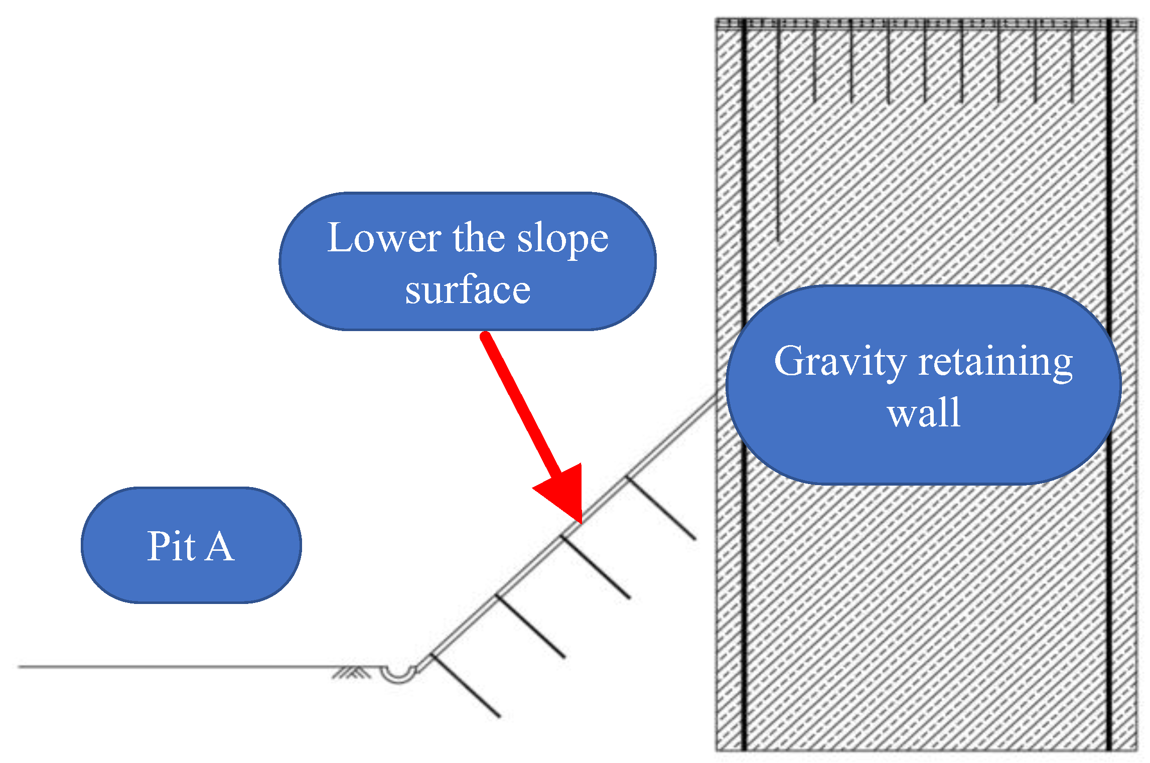
The data utilized in this study were obtained from the Phase II foundation pit project of Plot 027, Shangyong, Pazhou, Guangzhou (hereinafter referred to as “Pit A”). Situated in central Haizhu District, Guangzhou, Pit A lies to the west of Guangzhou Avenue and to the south of Yijing Road. The site is characterized by flat topography with minimal relief, featuring an absolute ground elevation of approximately 5.8–6.7 m. The excavation depth of Pit A ranges from 10.7 m to 11.6 m, with a total support perimeter measuring approximately 555 m. The construction employed a benched excavation method, supported by a lattice-type cement-mixed pile gravity retaining wall system, and was assigned a safety grade of Level 2. The general layout of the foundation pit is presented in Figure 1, and a typical cross-section of the support system is provided in Figure 2.
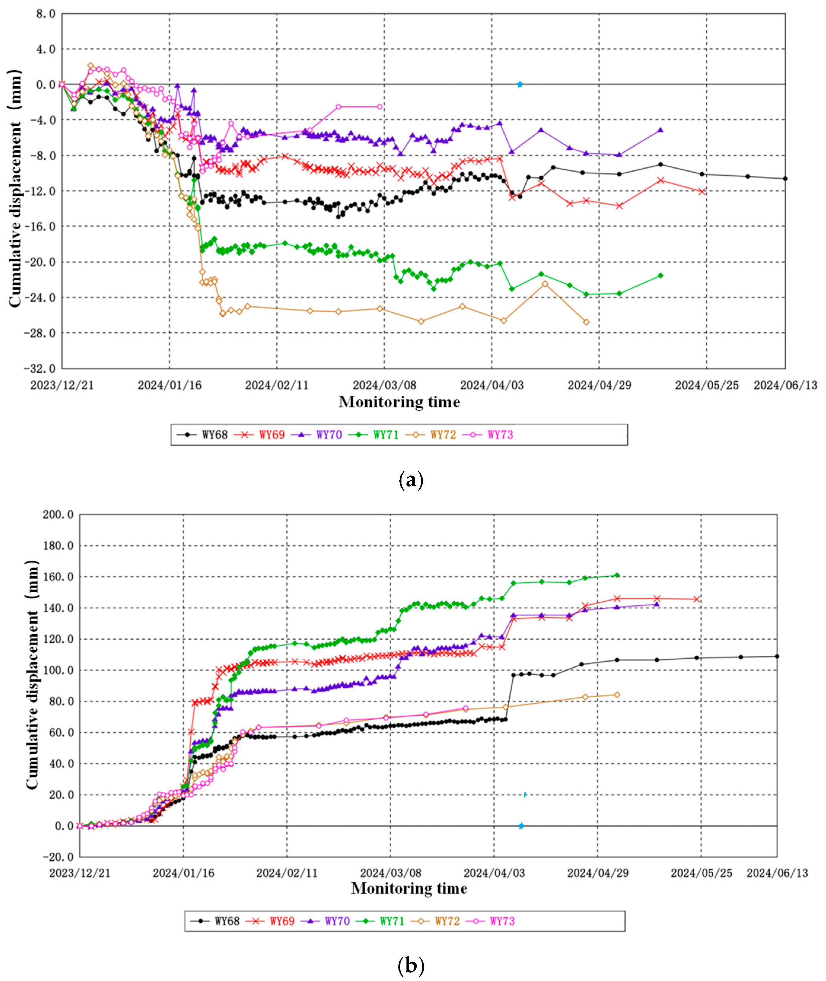
According to the detailed geotechnical investigation report for Pit A, the strata within the excavation range, from top to bottom, are primarily composed of plain fill, silty clay, silty clay, and residual silty clay. The surface fill and muddy silt layers are relatively thin, indicating favorable geological conditions. During the excavation of Pit A, various monitoring points including surface monitoring points, structural monitoring points, and stress monitoring points were installed along the perimeter. Monitoring was conducted once per day, with the frequency increased during earth excavation, heavy rainfall, or upon detection of abnormal deformations. The data used in this study include hydrogeological parameters of the construction area, excavation depth, groundwater level, as well as vertical and lateral displacements of the retaining structure. Detailed displacement data of the retaining structure can be found in Figure 3b.

2.2. Machine Learning Methods

2.2.1. Machine Learning Model

To predict the lateral displacement of the retaining structure, six common and effective machine learning models were selected to evaluate their predictive capabilities.
Decision Tree (DT) [20] is a recursively structured model based on feature partitioning. It constructs a tree-like architecture to divide the input space into multiple sub-regions for classification or regression tasks. The fundamental idea involves selecting the optimal feature as the splitting node and partitioning the samples according to specific criteria (e.g., information gain, Gini index) until a stopping condition is met. A typical decision rule is given by Equation (1).
f ( x ) = m = 1 M   c m I ( x R m )
where R m denotes the m-th region, c m is its corresponding output value, and I ( ) represents the indicator function.
Random Forest (RF) [21] is an ensemble learning method that combines multiple decision trees to reduce variance and enhance generalization capability. During the training phase, each tree is trained on bootstrap-sampled data (out-of-bag), and node splitting is performed only on a randomly selected subset of features, thereby promoting model diversity. The final output is based on an averaging strategy (for regression) as shown in Equation (2).
f ^ R F ( x ) = 1 T t = 1 T   f t ( x )
where T represents the number of trees, and f t ( x ) denotes the prediction result of the t-th tree.
K-Nearest Neighbors (KNN) [22] is a lazy learning algorithm that requires no explicit training process. The fundamental idea is: for a given test sample, compute its distance to all training samples, select the K nearest neighbors with the smallest distances, and predict the output based on voting or weighted averaging of the labels of these neighbors.
Support Vector Machine (SVM) [23] aims to find an optimal hyperplane in the feature space to achieve maximum-margin classification, which is inherently a convex optimization problem.
XGBoost [24] is an enhanced gradient boosting decision tree (GBDT) algorithm, featuring advantages such as regularization control, pruning, and parallel computing. The model constructs new trees sequentially to fit the residuals, continuously optimizing the objective function as shown in Equation (3):
L ( t ) = i = 1 n   l ( y i , y ^ i ( t 1 ) + f t ( x i ) ) + Ω ( f t )
where L ( t ) denotes the overall objective function at the t-th iteration, n is the total number of samples, y i is the true label value of the i-th sample, y ^ i ( t 1 ) is the predicted value of the i-th sample from the previous t 1 iteration, f t ( x i ) is the prediction of the t-th tree for sample x i , l ( ) is the loss function, and Ω f t is the regularization term.
LightGBM [25] is an efficient tree model based on the gradient boosting framework. It adopts a leaf-wise growth strategy and a histogram-based feature splitting algorithm, significantly improving training speed and memory efficiency. Compared to the level-wise growth approach of traditional GBDT, LightGBM is more capable of capturing complex nonlinear features.

2.2.2. SSA Optimization Algorithm

The Sparrow Search Algorithm (SSA) is a swarm intelligence optimization algorithm inspired by the foraging and anti-predation behaviors of sparrow populations. It achieves global optimization by simulating the cooperation and competition mechanisms among three roles in the sparrow population: finders, followers, and vigilantes.
Implementation steps of the algorithm:
Step 1: Initialize the sparrow population’s position information and fitness function, as well as the initial values of parameters such as the number of iterations N required by the algorithm, the number of individuals in the sparrow population n, the number of finders P D , the number of early-warning individuals S D , the safety threshold S T , and the early-warning value R 2 .
Step 2: Start cyclic iteration.
Step 3: Sort the population to obtain the current best sparrow position and fitness information.
Step 4: Update the positions of the finders.
X i , j t + 1 = X i , j t · e x p i · N           i f   R 2 < S T X i , j t + Q · L                                 i f   R 2 S T
where t is the number of iterations that have been performed, j = 1,2 , 3 , d . X i j is a high-dimensional array representing the position of the individual with serial number i in each dimension. Q represents a random value simulating the population position, and this value follows a normal distribution. L is a 1 × d unit row vector, and is any value between 0 and 1. N is the maximum number of iterations. R 2 0,1 and S T 0.5,1.0 .
Step 5: Update the positions of the joiners.
X i , j t + 1 = Q · e x p X w o r s t X i , j t i 2                     i f   i > n / 2 X p t + 1 + X i , j t X p t + 1 · A + · L     o t h e r w i s e
where X p t + 1 is the best position occupied by the discoverer in the current generation, and X w o r s t is the worst foraging location in the sparrow population, i.e., the position of the sparrow with the lowest fitness. A represents a 1 × d matrix with random values of 1 and −1, and A + = A t A A T 1 .
Step 6: Anti-predation, update the position of the sparrow population.
X i , j t + 1 = X b e s t t + β · X i , j t X b e s t t                             i f   f 1 > f b e s t X i , j t + K · X i , j t X w o r s t t f i f w o r s t + ε             i f   f 1 = f b e s t
where β is a random number that follows a normal distribution, and its function is to control the interval of position updates. K is a random number between [−1,1], and f i is the fitness value of each sparrow in this iteration. ε is a non-zero value to prevent the denominator from being zero.
Step 7: Update the historical optimal fitness.
Step 8: cyclically execute steps 3 to 7 until the current number of iterations reaches N , then end the loop. Output the highest fitness and its corresponding individual position.
The Sparrow Search Algorithm is used to optimize the initial weights and thresholds of the model. The optimization algorithm program obtains the fitness of SSA by calculating the M S E of the training data and test data, and the fitness is set as:
f i t n e s s = a r g m i n m s e T r a i n + m s e T e s t
where m s e T r a i n and m s e T e s t represent the predicted mean square errors obtained from the training and testing processes, respectively. A lower fitness indicates that the finally obtained network has a better prediction effect on the dataset.

2.2.3. SHAP-Based Explainable Analysis of Machine Learning Model Performance Evaluation

SHAP (SHapley Additive exPlanations) is a game theory-based model interpretation method used to explain predictions made by machine learning models. By quantifying the contribution of each feature to the model’s prediction, it helps elucidate the decision-making logic of the model. SHAP treats all micro-level parameters as “contributors,” with its core idea being to compute the marginal contribution of each micro-level parameter to the macro-level parameters, thereby providing visual explanations of the model’s predictions from both global and local perspectives. The equation for calculating the Shapley value, derived from cooperative game theory, is given by Equation (8).
φ i = S { x 1 , . . . , x M x i }   | S | ! M | S | 1 ! M ! ( f ( S { x i } ) f ( S ) )
where x i represents the input features, M is the total number of features, and S is the combination of all possible feature subsets excluded x i .

2.2.4. Performance Evaluation of Machine Learning Models

In this study, three measurement indicators are used to evaluate the proposed model: the coefficient of determination ( R 2 ), root mean square error ( R M S E ), and mean absolute error ( M A E ). These three indicators are defined as follows:
M A E = 1 k i = 1 k y i a y i p
R M S E = 1 k i = 1 k ( y i a y i p ) 2
R 2 = 1 i = 1 k y i a y i p 2 i = 1 k y i a y i a 2
where k is the total number of samples; y i p , y i a and y i a are predicted value, true value and average of the true value, respectively.
Smaller M A E and R M S E values indicate higher prediction accuracy of the model. The value of R 2 ranges from 0 to 1, and the closer it is to 1, the higher the prediction accuracy.

2.3. Data Partitioning and Modeling Workflow

2.3.1. Data Partitioning

To construct a complete dataset suitable for machine learning, the authors adopted a linear interpolation approach to address the “blank-day” issue commonly observed in real engineering monitoring records. First, all raw monitoring data were aligned according to their recording dates, and piecewise linear interpolation was applied between two adjacent measured values to fill in the missing dates within each interval. It should be noted that interpolation was performed only within the time span covered by actual measurements, without any extrapolation beyond the earliest or latest monitoring date, thereby avoiding the introduction of unrealistic artificial trends. After interpolation, a total of 83 data samples were obtained, with each sample containing the following variables: excavation depth S _ 1 (m), groundwater level S _ 2 (m), vertical displacement of the retaining structure Y _ 1 (mm), and horizontal displacement of the retaining structure X _ 1 (mm). Linear interpolation effectively captures the generally smooth and gradually nonlinear deformation characteristics during the excavation process, and it is a commonly used and rational simplification method in geotechnical monitoring and analysis. It provides an approximate representation of continuous deformation while mitigating the influence of uneven monitoring intervals.
Before model training, all input and output variables were normalized using Min–Max scaling, mapping them into the [0, 1] interval. The normalization formula is as follows:
x = x x m i n x m a x x m i n
where x is the original variable value, x is the normalized value, x m i n and x m a x denote the minimum and maximum values of the variable within the training set, respectively.
After obtaining the normalized prediction x p r e d from the model, the following denormalization formula is applied to map it back to its actual physical scale, ensuring that engineering quantities such as displacement retain their real units:
x p r e d = x p r e d ( x m a x x m i n ) + x m i n

2.3.2. Modeling Workflow

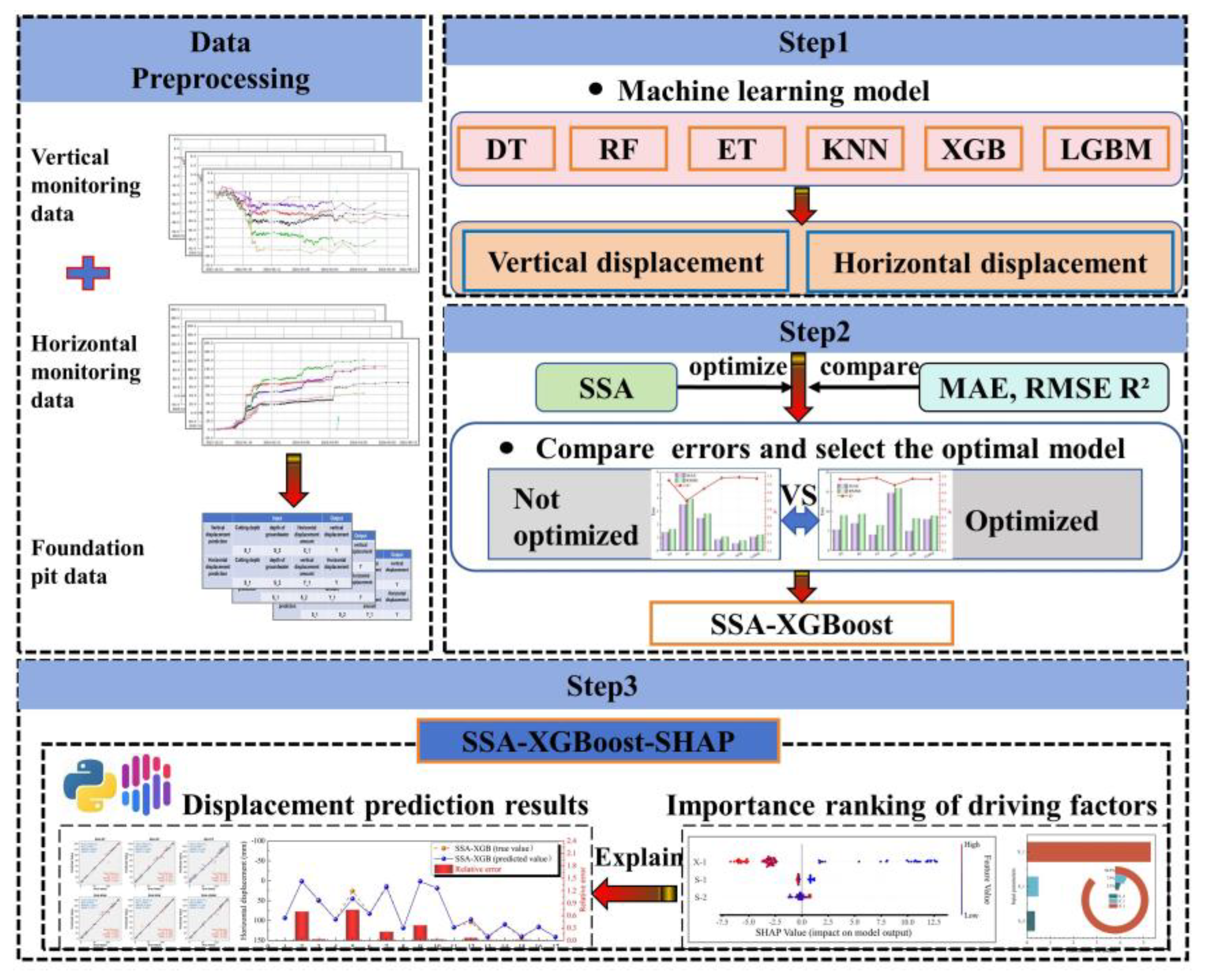
To achieve accurate prediction of shallow foundation settlement, this study proposes an interpretable machine learning (ML)-based approach. Each step of the proposed workflow is designed to enhance both the predictive accuracy and interpretability of the model—from data preparation and hyperparameter optimization to model evaluation and feature attribution analysis. As illustrated in Figure 4, the methodology integrates conventional ML algorithms, intelligent optimization techniques, and advanced explainable AI tools to construct a robust predictive framework. The process is summarized as follows:
Step 1: Real-world settlement data were obtained through field monitoring of a deep excavation project. The dataset was partitioned into two disjoint subsets: a training set and a testing set. The training data were used for model development, with prediction tasks focusing separately on vertical displacement ( Y _ 1 ) and horizontal displacement ( X _ 1 ). For vertical displacement prediction, the input features included excavation depth ( S _ 1 ), groundwater level ( S _ 2 ), and the observed horizontal displacement ( X _ 1 ). Conversely, for horizontal displacement prediction, the observed vertical displacement ( Y _ 1 ) was included as a key input feature. This design reflects the coupled behavior of vertical and horizontal deformations during soil-structure interaction, improving model performance while avoiding feature redundancy. Following the data partitioning strategy suggested by Nguyen et al. [45], the dataset was split in an 80%:20%, which has been shown to yield optimal training/testing performance for ML models.
Step 2: Six baseline ML models—DT, RF, ET, KNN, XGB, and LightGBM—were employed to predict both vertical and horizontal displacements. To further enhance model performance and convergence, the SSA was utilized to optimize the hyperparameters of each model. The integration of SSA with individual models led to the formation of hybrid models: SSA-DT, SSA-RF, SSA-ET, SSA-KNN, SSA-XGB, and SSA-LGBM. Comparative evaluations based on RMSE, MAE, and R2 were conducted to identify the best-performing model.
Step 3: To enhance interpretability, the SHAP method was applied to the optimal model. This allowed for a comprehensive interpretation of model predictions and facilitated a better understanding of how individual input variables influenced foundation settlement. By translating the “black-box” prediction process into intuitive and visualizable insights, SHAP enabled transparent decision-making and revealed the underlying engineering mechanisms.

3. Results

This study employed six distinct machine learning models—DT, RF, ET, KNN, XGB, and LGBM—to predict ground displacement during excavation, including both vertical and horizontal displacements. To improve the prediction accuracy and generalization ability of these models, the SSA was adopted to optimize their key hyperparameters, resulting in six hybrid models: SSA-DT, SSA-RF, SSA-ET, SSA-KNN, SSA-XGB, and SSA-LGBM. To evaluate model performance, three statistical metrics were used: the R2 to assess goodness-of-fit, the RMSE to quantify prediction deviations, and the MAE to measure the average prediction error. The results provide a comprehensive comparison of model performance, demonstrating both the relative strengths of each model and the effectiveness of SSA optimization in enhancing predictive capability for excavation-induced displacement. These findings offer meaningful insights for future applications in geotechnical displacement modeling.

3.1. Prediction Results of Displacement

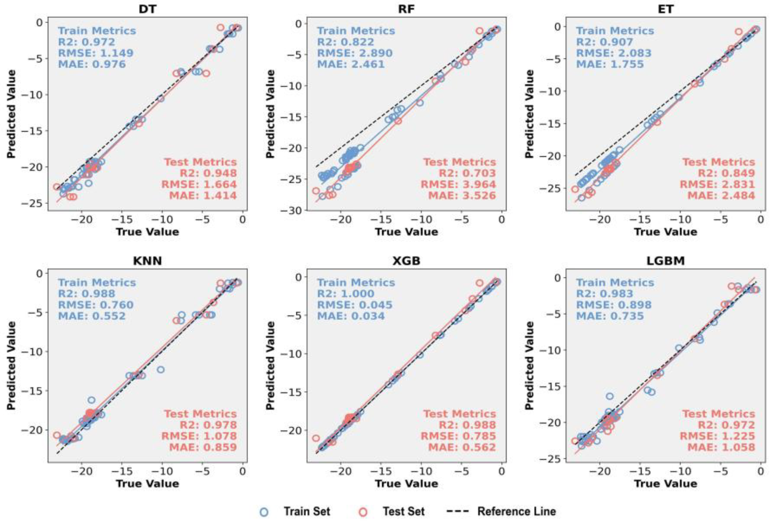
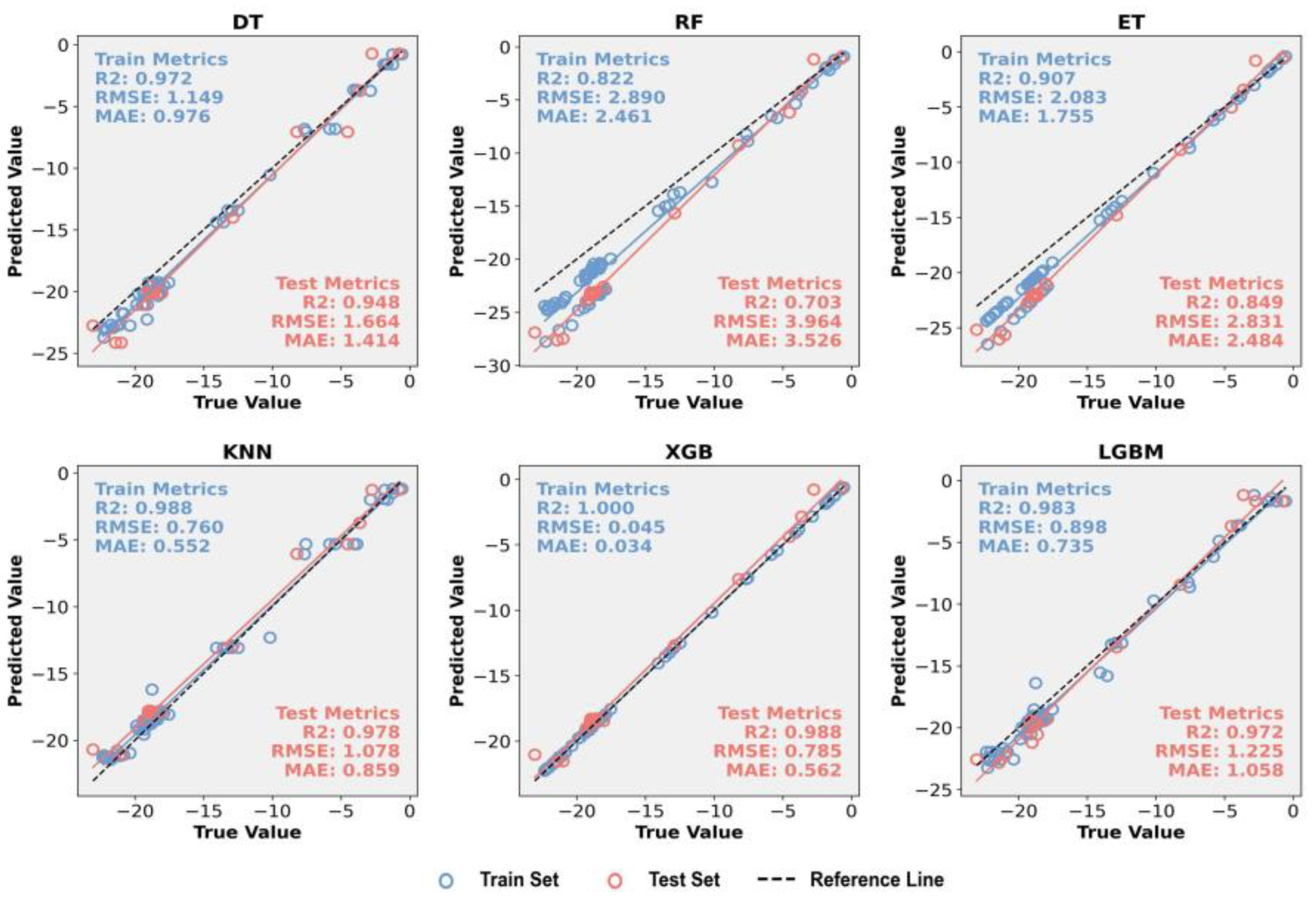
This section presents the prediction performance of six unoptimized machine learning models for vertical displacement in excavations. In the Figure 5, the dotted line is Ideal fitting line ( y = x ), the solid red is regression line for test data, the solid blue is regression line for training data (the same below). The XGB model demonstrates the highest predictive accuracy among the unoptimized models for vertical displacement prediction, achieving a perfect fit on the training set ( R 2 = 1.000) and excellent generalization on the testing set ( R 2 = 0.988). It also achieves the lowest error metrics among all models, with R M S E and M A E values of 0.045 and 0.034 on the training set, and 0.785 and 0.562 on the testing set, respectively. This indicates strong fitting capacity and robust generalization. KNN and LGBM also perform reasonably well. In contrast, RF and ET models show relatively lower predictive accuracy, particularly RF, which yields the lowest testing R 2 (0.703) and the highest errors.
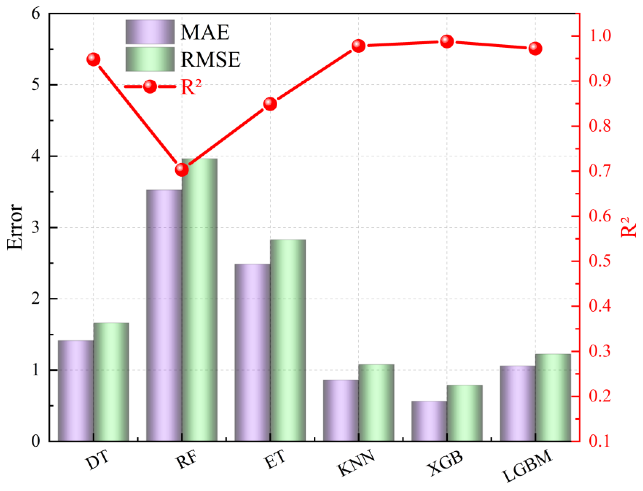
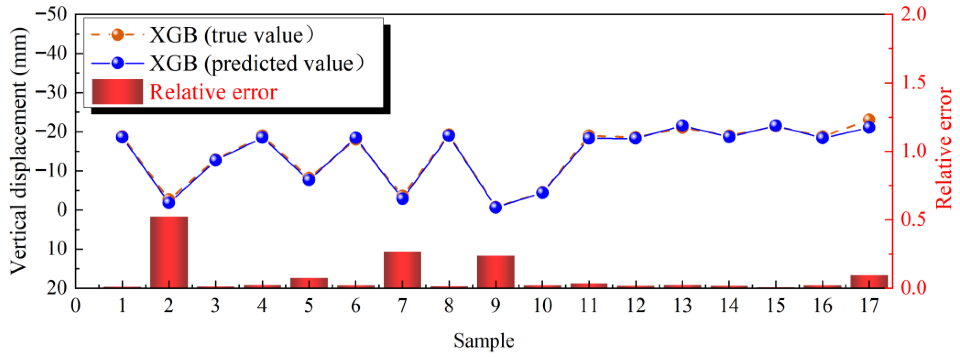
Figure 6 and Table 1 provide a direct comparison of error metrics across all models. The XGB model clearly achieves the lowest R M S E and M A E , confirming its superior accuracy and robustness. Figure 7 shows the predicted versus actual vertical displacements for 17 testing samples using the XGB model, along with their relative errors. The predicted values closely follow the actual values, and most samples exhibit relative errors below 10%, indicating stable and reliable predictions. This highlights the model’s potential for practical geotechnical applications.
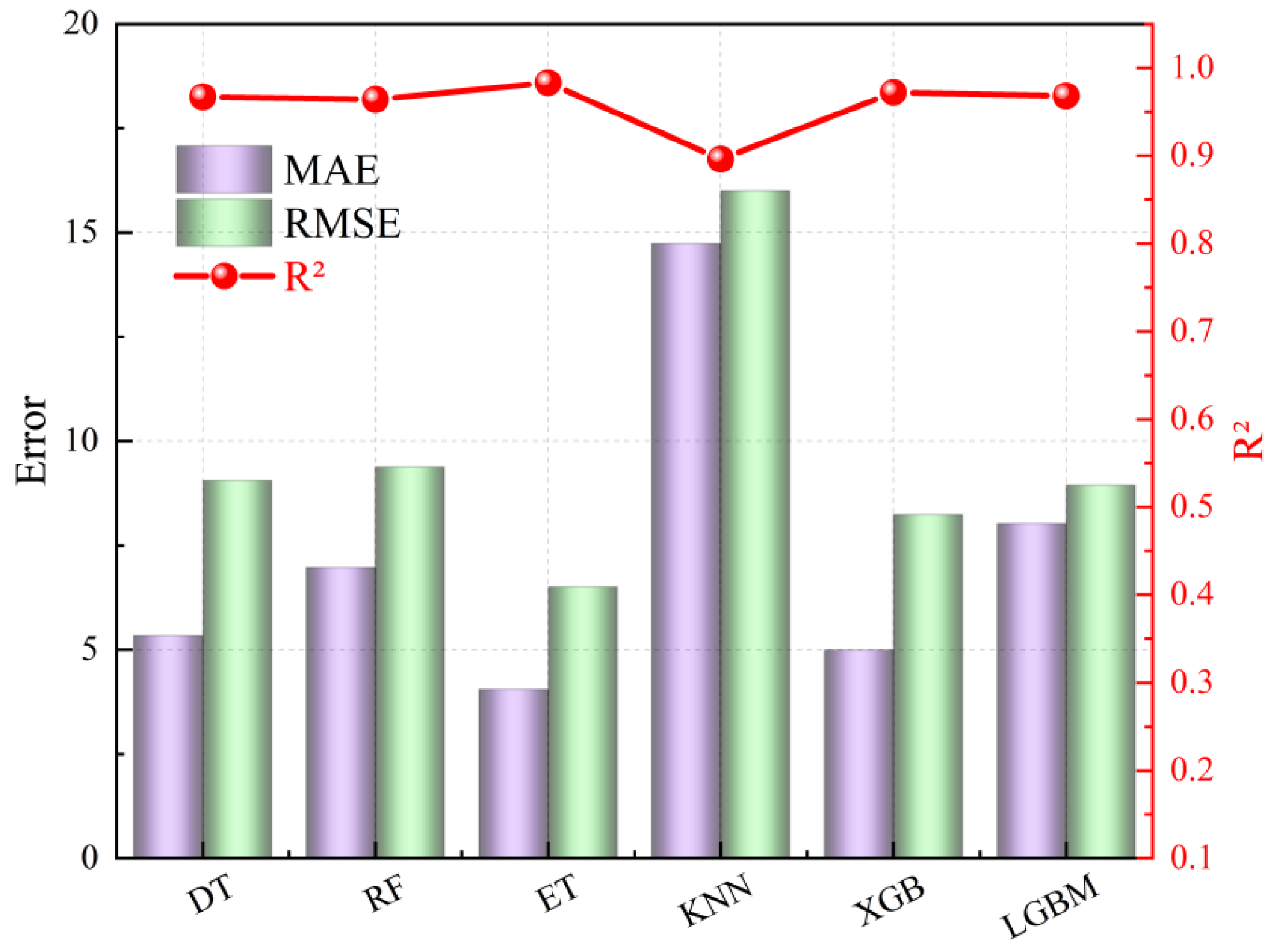
In addition, Figure 8 presents the prediction performance of six unoptimized models for horizontal displacement during excavation. As shown in Figure 8, the ET model achieves outstanding accuracy, with perfect fitting on the training set ( R 2 = 1.000, R M S E = 0.002, M A E = 0.001) and excellent generalization on the testing set ( R 2 = 0.983, R M S E = 6.508, M A E = 4.046). The DT and XGB models also perform well, with test R 2 values of 0.967 and 0.972, respectively. In contrast, the KNN model exhibits the poorest predictive performance, with a testing R 2 of only 0.896 and significantly higher R M S E (16.002) and M A E (14.736), indicating limited capability in capturing feature interactions.
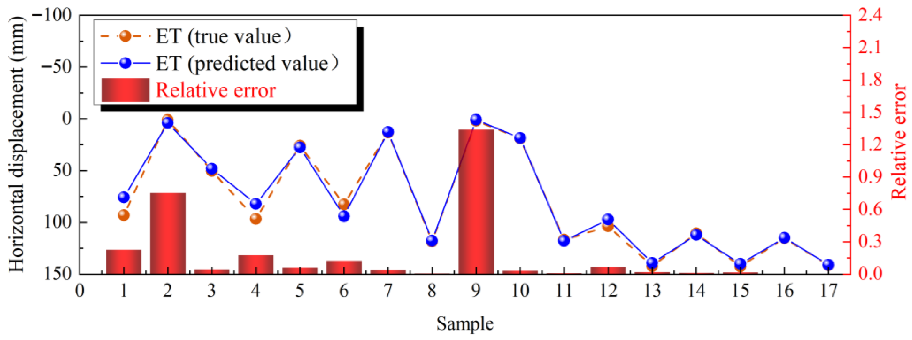
Figure 9 and Table 2 further visualize the prediction errors across models. The ET model demonstrates the highest M A E and R M S E values, confirming its superior prediction accuracy and robustness. Meanwhile, the KNN model shows the lowest prediction errors, reflecting its relatively poor stability. Figure 10 illustrates the ET model’s predictions versus actual horizontal displacements on 17 testing samples. Overall, the predicted values align well with the true values, and most samples exhibit low relative errors. Although larger deviations are observed for certain samples (e.g., Sample 2 and Sample 9), the majority show high accuracy, suggesting that the ET model is highly effective in modeling excavation-induced horizontal displacement.

3.2. Displacement Prediction Results of SSA-Optimized Models

To improve the accuracy and generalization ability of foundation pit displacement prediction, this study employs six mainstream machine learning models: DT, RF, ET, KNN, XGB, and LGBM. The SSA was introduced to automatically optimize the key hyperparameters of each model. By comparing the predictive performance of the original models and their optimized hybrid counterparts (SSA-DT, SSA-RF, SSA-ET, SSA-KNN, SSA-XGB, SSA-LGBM), the enhancement effect of hyperparameter tuning on model accuracy was systematically evaluated.
During the optimization process, SSA was applied to search and adjust the core hyperparameters that significantly influence the performance of each model. The selected parameters were determined based on empirical rules and preliminary experimental analysis. Among these parameters, L 2 regularization penalizes excessively large leaf weights, thereby suppressing overfitting to local fluctuations or noise in the monitoring data. In this study, the L 2 regularization parameter is set to 1.0. The main hyperparameters optimized by SSA for each model, along with their final values, are listed in Table 3.
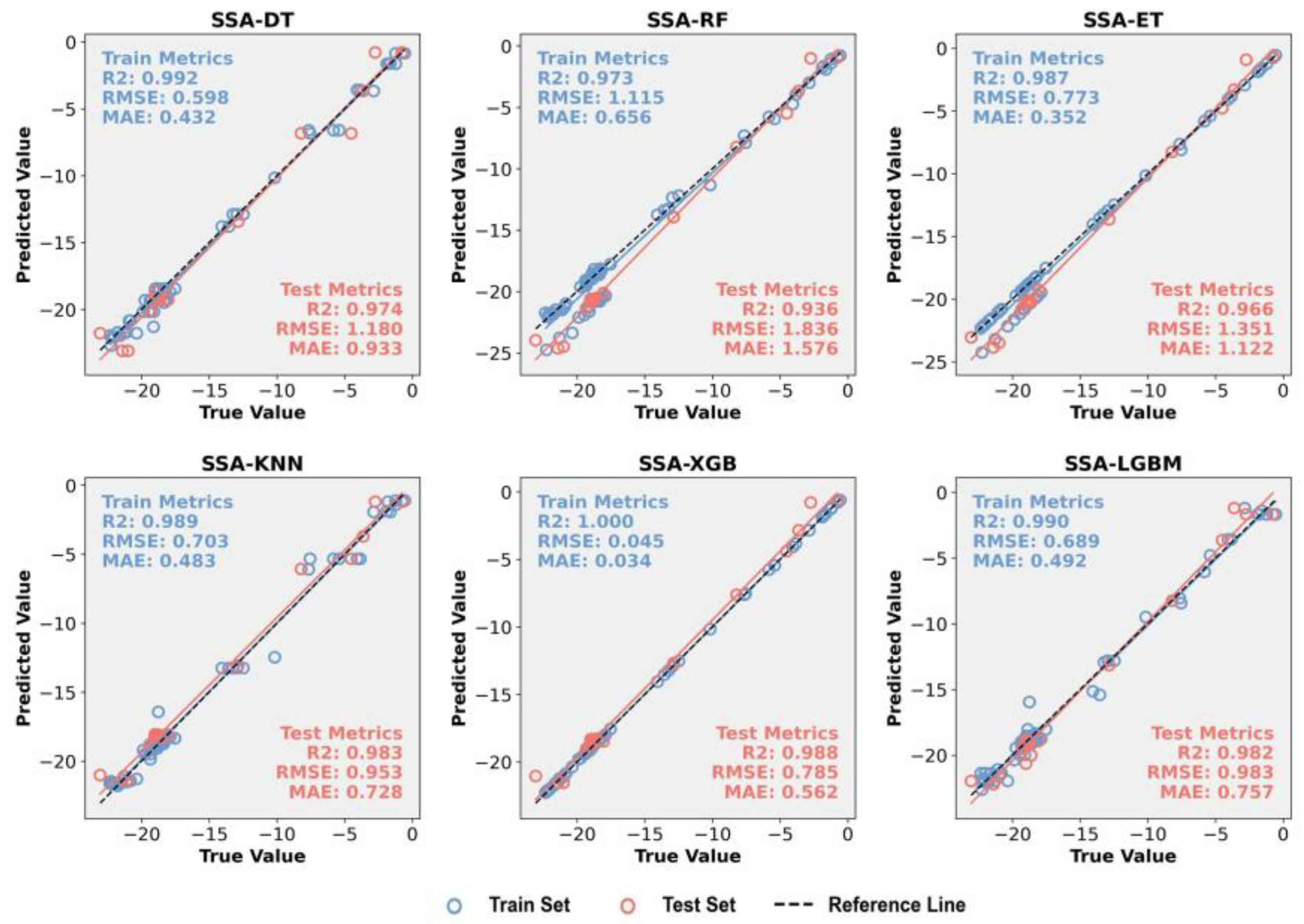
The predicted results of vertical displacement using the SSA-optimized models are shown in Figure 11, Figure 12 and Figure 13. As shown in Figure 11, all SSA-optimized models exhibit improved predictive accuracy compared to their unoptimized counterparts. Notably, the SSA-XGB model achieves outstanding performance, with perfect fitting on the training set ( R 2 = 1.000) and strong generalization on the test set ( R 2 = 0.988). Its error metrics are the lowest among all models— R M S E of 0.045 and M A E of 0.034 on the training set, and R M S E of 0.785 and M A E of 0.562 on the test set—indicating excellent prediction capability and model stability. SSA-KNN, SSA-LGBM, and SSA-ET also perform well, with significant improvements over their unoptimized versions. Although SSA-RF still show relatively higher errors, their prediction accuracy is also enhanced after optimization.
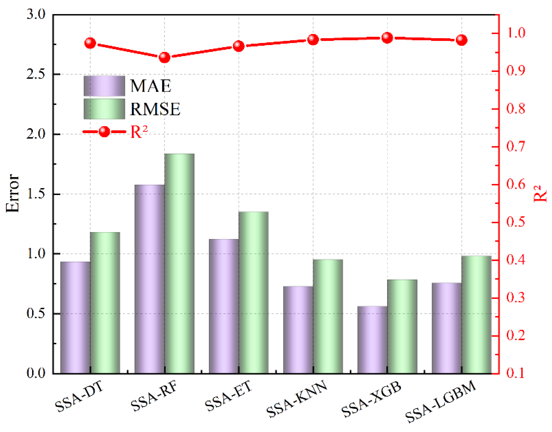
Figure 12 and Table 4 further illustrate the comparative performance using bar charts of R M S E and M A E on the test set. The SSA-XGB model demonstrates the lowest error values, confirming its superior robustness and precision. SSA-KNN and SSA-LGBM also show stable and reliable performance.
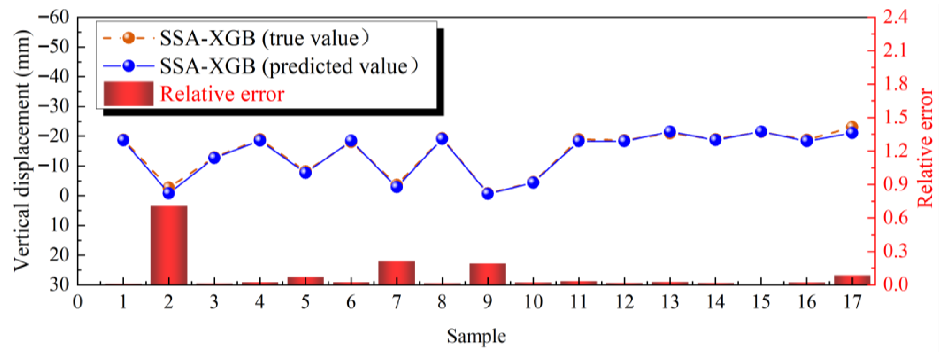
Figure 13 analyzes the detailed prediction results of the SSA-XGB model on 17 testing samples. The predicted displacement closely follows the actual values, with smooth and consistent trends. Except for a few cases (e.g., Sample 2) with slightly higher relative error, most samples exhibit minimal deviation, demonstrating the effectiveness of SSA in enhancing model reliability.
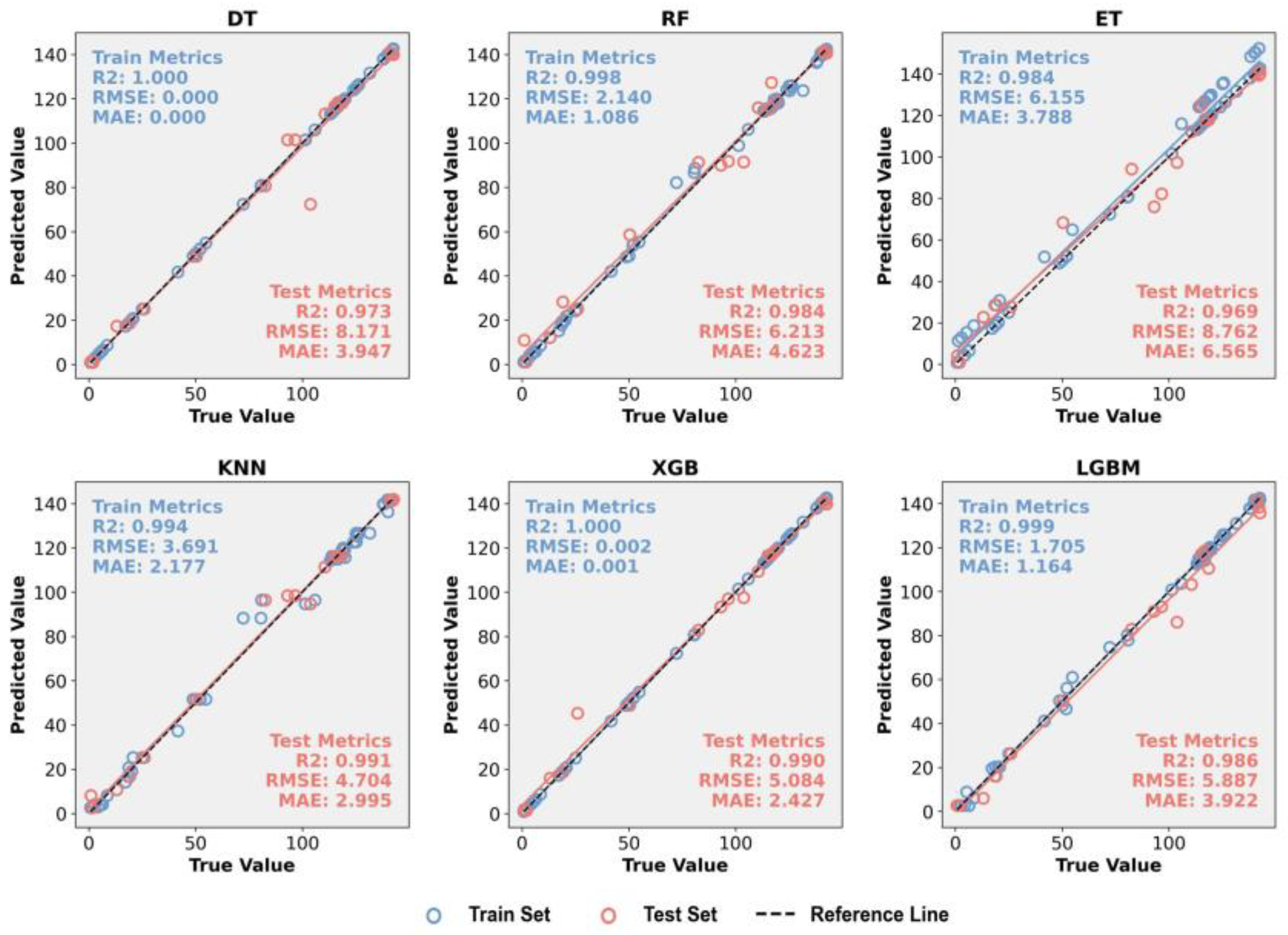
The predicted results of horizontal displacement using the SSA-optimized models are shown in Figure 14, Figure 15 and Figure 16. As shown in Figure 14, most SSA-optimized models exhibit considerable improvements in predictive performance. The SSA-XGB model achieves excellent results, with perfect training accuracy ( R 2 = 1.000) and a high testing R 2 of 0.990. It also attains relatively low error metrics on the test set ( R M S E = 5.084, M A E = 2.427). Although SSA-KNN and SSA-DT also show high R 2 values, their error values remain slightly higher (e.g., SSA-DT: R M S E = 8.171, M A E = 3.947). The SSA-ET and SSA-LGBM models show relatively larger prediction deviations in some cases, indicating limitations in capturing extreme or fluctuating data.
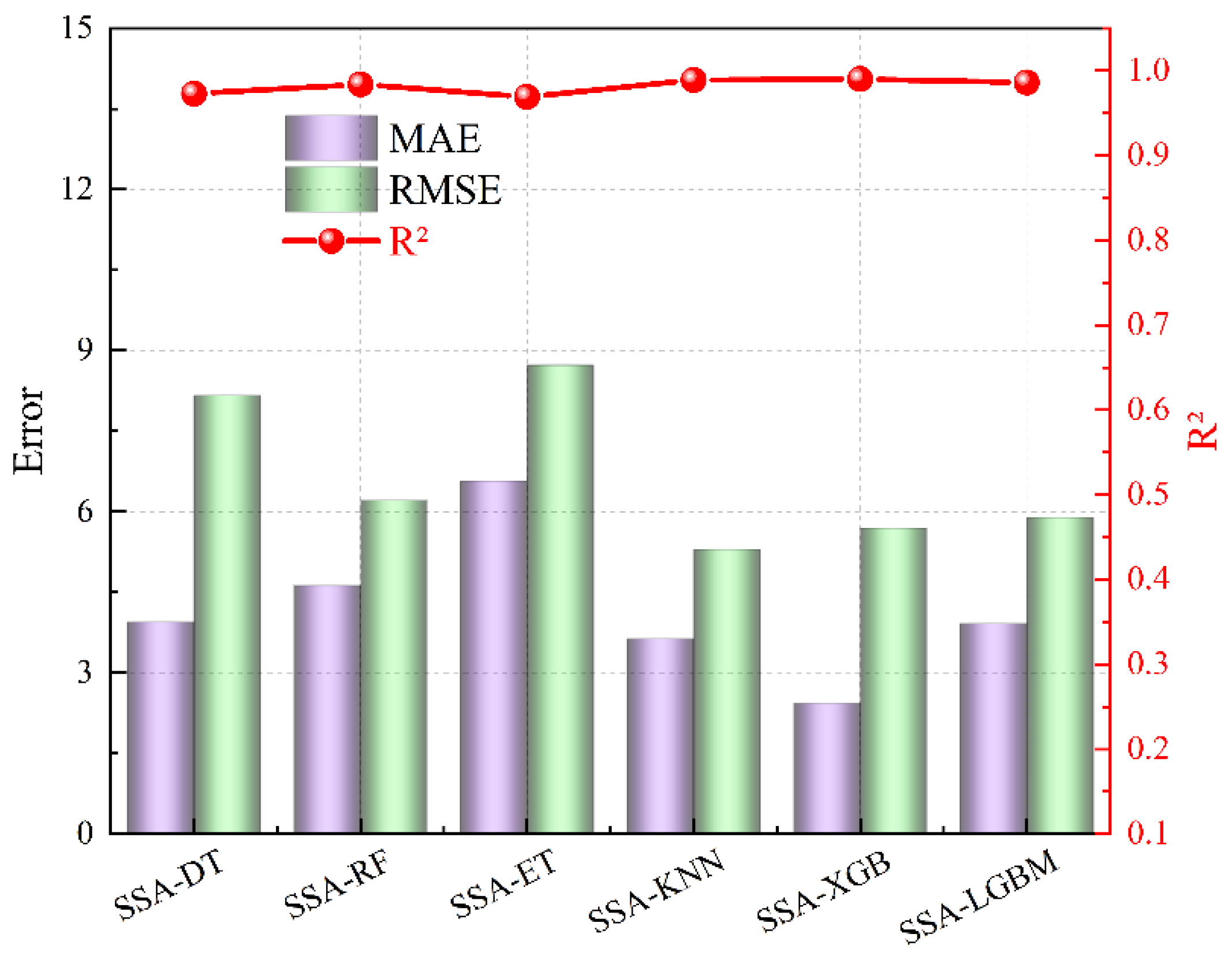
Figure 15 and Table 5 further highlight the performance differences using bar plots of R M S E and M A E . The SSA-XGB model outperforms all others with the lowest error values. Additionally, all models maintain R 2 values above 0.98, indicating reliable generalization after SSA-based optimization.
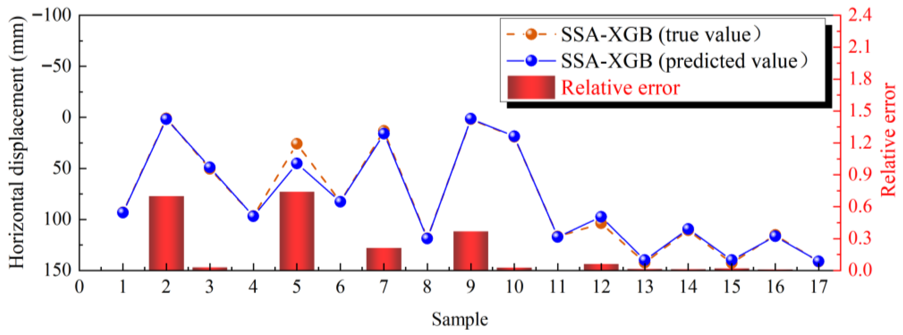
Figure 16 analyzes the SSA-XGB model’s performance across 17 test samples. The predicted values closely match the true values for most samples, with minimal relative errors observed particularly from Sample 6 to Sample 17. Slightly larger deviations occur at Sample 2 and Sample 5, but the overall predictive performance remains stable and robust. These results confirm the SSA-XGB model’s capability to accurately model horizontal displacement under complex geotechnical conditions.

3.3. SHAP-Based Interpretability Analysis

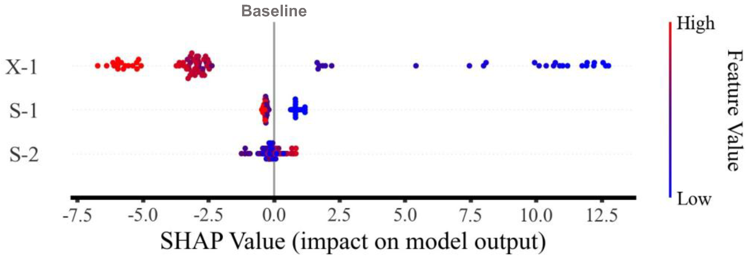
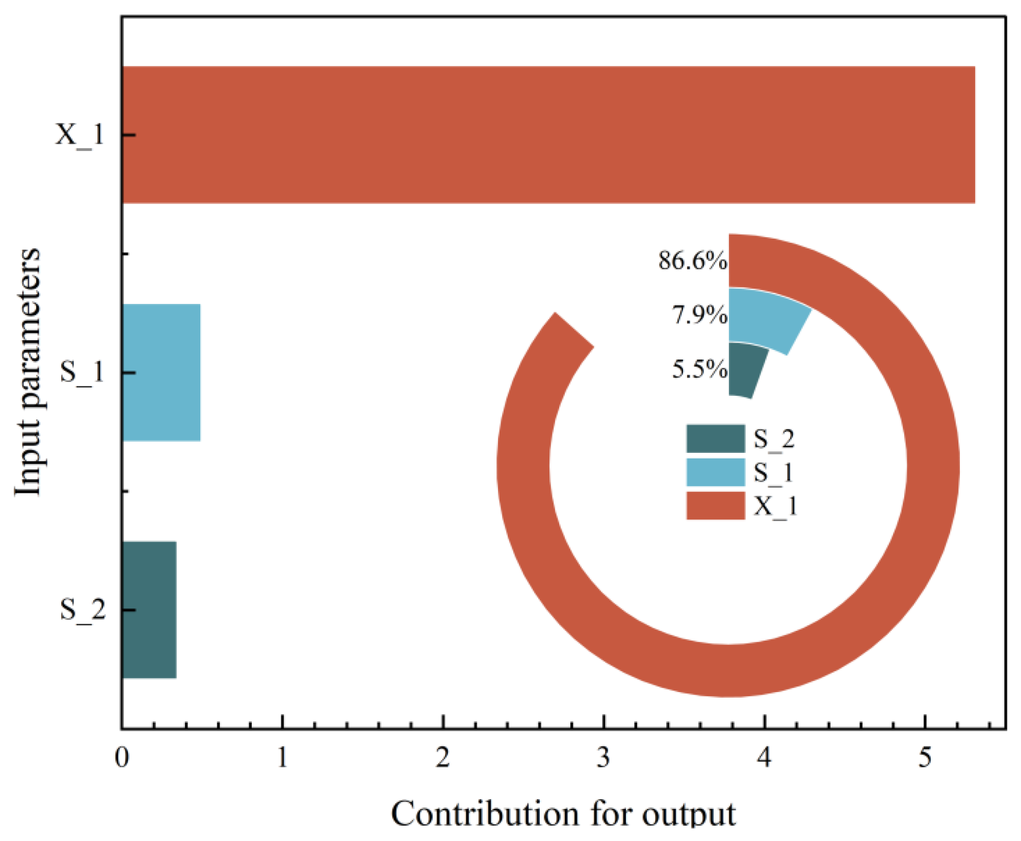
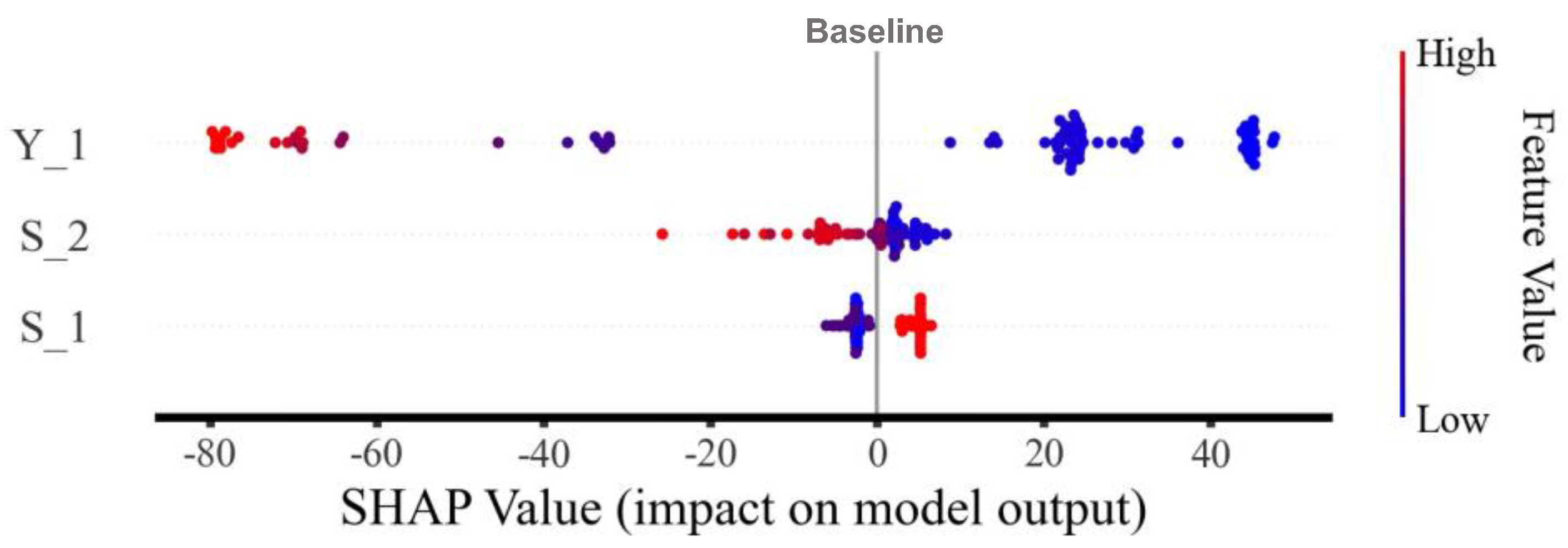
Figure 17, Figure 18, Figure 19 and Figure 20 present the feature importance analysis results for foundation pit displacement prediction using the SSA-XGB model. Figure 17 displays the SHAP values of the SSA-XGB model, illustrating the influence of each input feature on the model output. On the x-axis, the SHAP value indicates the extent to which each feature affects the predicted displacement: positive values suggest an increase in predicted settlement, while negative values indicate a decrease. Feature importance is visualized using a color gradient from blue (low feature values) to red (high feature values), showing how each feature’s magnitude contributes to model prediction.
As shown in Figure 18, the SHAP summary plot reveals that horizontal displacement ( X _ 1 ) has the most significant impact on the predicted vertical displacement. The SHAP value distribution indicates that higher values of X _ 1 correspond to more positive SHAP values, suggesting a strong positive contribution to vertical displacement prediction. This means that when the mid-height displacement of the retaining wall increases, the unloading of the soil behind the wall becomes more significant, leading to greater vertical settlement of the overlying soil. Similar trends have been reported in field observations and numerical back-analyses of deep excavations in soft clay, where larger wall deflections are associated with larger ground surface settlements [46]. In contrast, the SHAP values of excavation depth ( S _ 1 ) and groundwater level ( S _ 2 ) are mostly concentrated around zero, indicating a relatively minor influence on the prediction outcome, which is consistent with studies showing that, for a given project, ground surface settlement outside the excavation is mainly controlled by the magnitude of wall lateral displacement rather than small variations in groundwater level or excavation depth at a single stage [47].
As shown in Figure 19, the SHAP summary plot indicates that vertical displacement ( Y _ 1 ) is the most influential input variable for horizontal displacement prediction. The SHAP values of Y _ 1 exhibit a wide range of both positive and negative impacts: high values (shown in red) generally contribute significantly to increased prediction outputs, whereas low values (shown in blue) tend to suppress the model output. This suggests a strong co-evolutionary relationship between vertical and horizontal deformations. The occurrence of vertical settlement usually implies a reduction in soil stiffness and a change in the principal stress path, while the soil arching effect behind the retaining wall is weakened accordingly, making the wall more prone to additional horizontal displacement under the same external load. This coupled “vertical deformation–horizontal deformation” mechanism has been observed in excavation monitoring studies and database analyses, where the evolution of ground settlement profiles is closely linked to the pattern of wall deflection [46,48]. In contrast, the SHAP value distributions for excavation depth ( S _ 1 ) and groundwater level ( S _ 2 ) are more narrowly centered around zero, indicating relatively weak contributions to the model output.
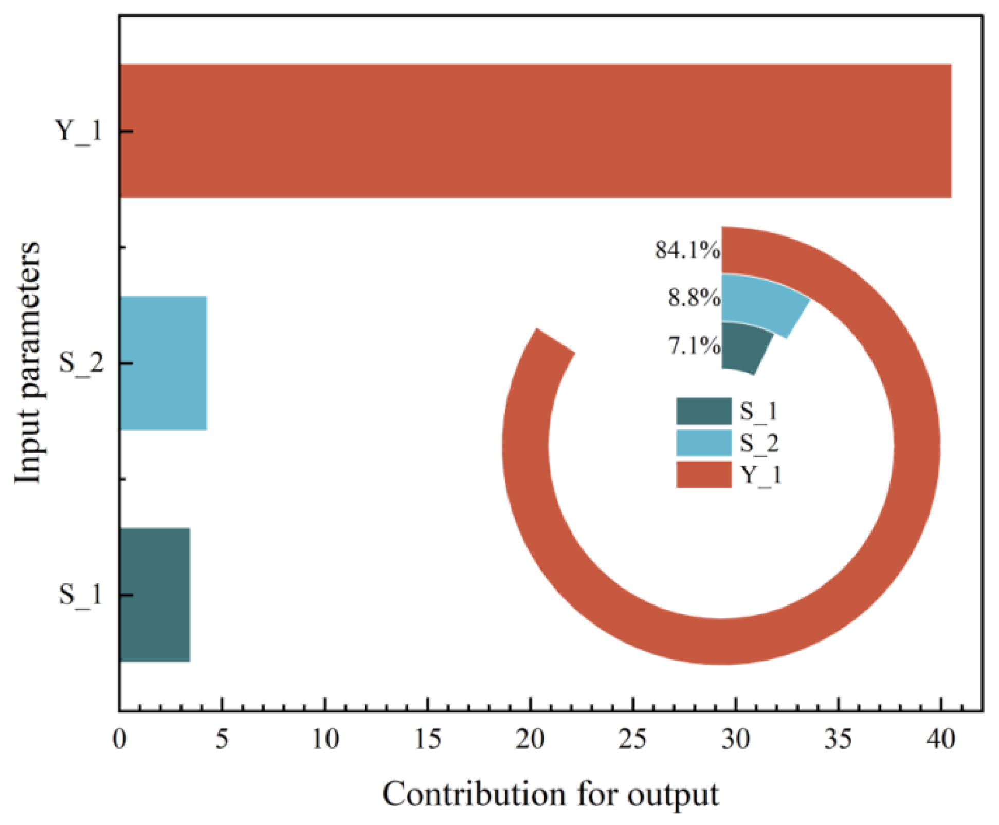
Figure 20 presents the quantitative analysis of input feature importance. The results show that vertical displacement ( Y _ 1 ) accounts for 84.1% of the model’s total contribution, which is significantly higher than that of groundwater level ( S _ 2 , 8.8%) and excavation depth ( S _ 1 , 7.1%). From an engineering perspective, this is because significant non-uniform unloading exists during excavation, and the deformation mode of the retaining structure together with progressive soil stiffness degradation governs the spatial distribution of earth pressure [49]. This distribution of contribution highlights that horizontal deformation during excavation is highly dependent on the response mechanism of vertical deformation, which may be associated with stress redistribution induced by excavation disturbance. In comparison, static geological factors such as S _ 1 and S _ 2 have limited explanatory power for horizontal displacement prediction when deformation feedback is absent, reflecting the complexity and dynamic nature of subsurface responses.

4. Discussion

The results presented in Section 3 demonstrate the effectiveness of the proposed SSA-XGB model in predicting both vertical and horizontal displacements during foundation pit excavation. This section provides a comprehensive discussion of these findings, focusing on model performance, the impact of hyperparameter optimization, the interpretability of predictions, and the practical implications for geotechnical engineering.
The results of this study demonstrate the effectiveness of the SSA-XGB model in predicting excavation-induced displacements, achieving R 2 values of 0.988 and 0.990 for vertical and horizontal displacements, respectively. These outcomes are notably superior to those reported in several recent studies. For instance, Zhang et al. [29] applied artificial neural networks to predict ground settlement but achieved lower accuracy ( R 2 ≈ 0.92–0.95) under similar geotechnical conditions. Similarly, Che Mamat [30] used SVM models for maximum surface settlement prediction but encountered limitations in handling nonlinear inter However, it is noteworthy that hyperparameter optimization did not uniformly improve all models. For instance, the unoptimized ET model outperformed its SSA-optimized counterpart in predicting horizontal displacement. This suggests that in noisy or data-limited environments, simpler models may sometimes generalize better due to their inherent structural simplicity and lower sensitivity to parameter variations. This finding echoes the observations of [36], who noted that excessive tuning could lead to overfitting in certain scenarios.
The SHAP-based interpretability analysis revealed a strong mutual dependency between vertical and horizontal displacements. Horizontal displacement ( X _ 1 ) was the most influential feature in predicting vertical displacement, while vertical displacement ( Y _ 1 ) was the dominant factor in predicting horizontal displacement. This bidirectional coupling reflects the complex soil-structure interaction during excavation, where stress redistribution and deformation mechanisms are inherently linked. Such insights are consistent with classical geotechnical theories [4,5] and underscore the importance of considering multi-directional displacement feedback in predictive modeling.
From a practical standpoint, the high contribution of displacement feedback features ( X _ 1 and Y _ 1 ) over static factors like excavation depth ( S _ 1 ) and groundwater level ( S _ 2 ) suggests that real-time monitoring data play a crucial role in accurate displacement prediction. This supports the shift from passive monitoring to proactive intelligent control in modern geotechnical engineering. The SSA-XGB model, with its high accuracy and interpretability, offers a reliable tool for early warning systems and risk management in deep excavation projects.
In summary, the proposed SSA-XGB model not only achieves high predictive accuracy but also offers transparent and interpretable outputs, making it a valuable asset for intelligent decision-making in foundation pit engineering. actions among multiple influencing factors.

5. Conclusions

This study presents a scientifically novel and interpretable machine learning framework for predicting excavation-induced displacements, integrating the Sparrow Search Algorithm (SSA) with the XGBoost model to enhance both predictive accuracy and model transparency. The main scientific contributions and quantitative findings are summarized as follows:
(1) The SSA-XGB hybrid model achieved the highest prediction accuracy among all tested models, with R2 = 0.988 for vertical displacement and R 2 = 0.990 for horizontal displacement. The corresponding error metrics were also the lowest ( R M S E = 0.785, M A E = 0.562 for vertical; R M S E = 5.684, M A E = 2.427 for horizontal), demonstrating the model’s robustness and generalization capability under complex geotechnical conditions.
(2) A key scientific novelty lies in the integration of SSA for hyperparameter optimization, which systematically enhanced the performance of most baseline models. However, it was also found that hyperparameter tuning does not universally improve performance; in some cases (e.g., ET models), the unoptimized versions performed better, highlighting the context-dependent nature of model optimization.
(3) Through SHAP-based interpretability analysis, the study quantitatively revealed a strong coupling between vertical and horizontal displacements. Horizontal displacement ( X _ 1 ) was the most influential feature in predicting vertical displacement, while vertical displacement ( Y _ 1 ) contributed 84.1% of the total feature importance in horizontal displacement prediction. This mutual dependency provides new insights into the coupled deformation mechanisms in excavation engineering.
Future research will focus on extending the proposed model to multi-output prediction tasks while explicitly incorporating temporal effects. In addition, integrating physical knowledge with data-driven machine learning approaches may help overcome the limitations in model generalization caused by the scarcity of monitoring data.

Author Contributions

Conceptualization, G.Y.; Methodology, G.Y. and F.Z.; Software, A.Y. and Q.F.; Validation, D.G.; Visualization, F.Z. and D.G.; Formal analysis, G.Y. and D.G.; Investigation, F.Z.; Resources, G.Y. and Z.H.; Data curation, A.Y. and Q.F.; Supervision, Q.F. and Z.H.; Writing—original draft, G.Y. and Q.F.; Writing—review & editing, Q.F. and Z.H.; Project administration, Q.F. and Z.H. All authors have read and agreed to the published version of the manuscript.

Funding

This research received no external funding. The APC was funded by [Z.H.].

Data Availability Statement

The original contributions presented in the study are included in the article, further inquiries can be directed to the corresponding authors.

Conflicts of Interest

Author Fan Zhang employed by the Guangdong Sheng Xiang Traffic Engineering Inspection Co., Ltd. Author Dianta Guo employed by the Guangdong Architectural Design and Research Institute Group Co., Ltd. Author Zhiwei He employed by the COBD Holdings (Guangzhou) Co., Ltd. The remaining authors declare that the research was conducted in the absence of any commercial or financial relationships that could be construed as potential conflicts of interest.

References

  1. Zhang, J.; Wang, H.; Huang, H.W.; Chen, Z. A Systematic Review of Urban Underground Space Development in China. Tunn. Undergr. Space Technol. 2023, 131, 104785. [Google Scholar] [CrossRef]
  2. Liu, J.; Li, T.; Yang, H. Challenges and Countermeasures of Deep Excavation in Soft Soil Areas of Coastal Cities. J. Perform. Constr. Facil. 2022, 36, 04022045. [Google Scholar] [CrossRef]
  3. Wang, Z.; Wang, L.; Li, L.; Wang, J. Deformation Characteristics of a 30-m Deep Excavation in Soft Clay. Comput. Geotech. 2021, 134, 104100. [Google Scholar] [CrossRef]
  4. Li, D.; Liao, F.; Wang, L.; Lin, J.; Wang, J. Multi-Stage and Multi-Parameter Influence Analysis of Deep Foundation Pit Excavation on Surrounding Environment. Buildings 2024, 14, 297. [Google Scholar] [CrossRef]
  5. Zhang, W.; Huang, Z.; Zhang, J.; Zhang, R.; Ma, S. Multifactor Uncertainty Analysis of Construction Risk for Deep Foundation Pits. Appl. Sci. 2022, 12, 8122. [Google Scholar] [CrossRef]
  6. Ou, C.Y. Deep Excavation: Theory and Practice; CRC Press: Boca Raton, FL, USA, 2014. [Google Scholar]
  7. Finno, R.J.; Blackburn, J.T.; Roboski, J.F. Three-Dimensional Effects for Supported Excavations in Clay. J. Geotech. Geoenviron. Eng. 2007, 133, 30–36. [Google Scholar] [CrossRef]
  8. Schuster, M.; Kung, G.T.C.; Juang, C.H.; Hashash, Y.M.A. Simplified Model for Evaluating Damage Potential of Buildings Adjacent to a Braced Excavation. J. Geotech. Geoenviron. Eng. 2009, 135, 1823–1835. [Google Scholar] [CrossRef]
  9. Liu, Y.; Zhang, D.; Huang, Z. A Probabilistic Risk Assessment Framework for Building Damage Induced by Adjacent Excavations. Reliab. Eng. Syst. Saf. 2023, 237, 109367. [Google Scholar] [CrossRef]
  10. Peck, R.B. Deep Excavations and Tunneling in Soft Ground. In Proceedings of the 7th International Conference on Soil Mechanics and Foundation Engineering, Mexico City, Mexico, 25–29 August 1969; pp. 225–290. [Google Scholar]
  11. Clough, G.W.; O’Rourke, T.D. Construction Induced Movements of Insitu Walls. In Design and Performance of Earth Retaining Structures; ASCE: Reston, VA, USA, 1990; pp. 439–470. [Google Scholar]
  12. Hsieh, P.G.; Ou, C.Y. Shape of Ground Surface Settlement Profiles Caused by Excavation. Can. Geotech. J. 1998, 35, 1004–1017. [Google Scholar] [CrossRef]
  13. Poulos, H.G.; Chen, L.T.; Hull, T.S. Model Tests on Single Piles Subjected to Lateral Soil Movement. Soils Found. 1995, 35, 85–92. [Google Scholar] [CrossRef]
  14. Xu, Z.; Wang, W.; Wang, J. Analytical Solution for Braced Excavation Deformation Considering Soil Stress History. Int. J. Geomech. 2022, 22, 04021280. [Google Scholar] [CrossRef]
  15. Brinkgreve, R.B.J.; Swolfs, W.M.; Engin, E. PLAXIS 2015; PLAXIS bv: Delft, The Netherlands, 2015. [Google Scholar]
  16. Potts, D.M.; Zdravkovic, L. Finite Element Analysis in Geotechnical Engineering: Theory; Thomas Telford: London, UK, 1999. [Google Scholar]
  17. Goh, A.T.C.; Kulhawy, F.H. Reliability Assessment of Basement Wall Movements Using Finite Element Method. J. Geotech. Geoenviron. Eng. 2005, 131, 1319–1331. [Google Scholar] [CrossRef]
  18. Kung, G.T.C.; Hsiao, E.C.L.; Schuster, M.; Juang, C.H. A Neural Network Approach to Estimating Deflection of Diaphragm Walls Induced by Excavation in Clays. Comput. Geotech. 2007, 34, 385–396. [Google Scholar] [CrossRef]
  19. Benz, T. Small-Strain Stiffness of Soils and Its Numerical Consequences; Universität Stuttgart: Stuttgart, Germany, 2007. [Google Scholar]
  20. Tschuchnigg, F.; Schweiger, H.F. The Embedded Pile Concept—Verification of an Efficient Tool for Modelling Deep Excavations. Comput. Geotech. 2015, 63, 244–253. [Google Scholar] [CrossRef]
  21. Phoon, K.K.; Kulhawy, F.H. Characterization of Geotechnical Variability. Can. Geotech. J. 1999, 36, 612–624. [Google Scholar] [CrossRef]
  22. Cao, Z.; Wang, Y.; Li, D. Bayesian Model Comparison and Characterization of Undrained Shear Strength for Clays. Eng. Geol. 2016, 203, 137–144. [Google Scholar] [CrossRef]
  23. Schweiger, H.F. Results from Numerical Benchmark Exercises in Geotechnics. In Proceedings of the 5th International Symposium on Numerical Models in Geomechanics, Davos, Switzerland, 6–8 September 1995; Balkema: Rotterdam, The Netherlands, 1992; pp. 225–232. [Google Scholar]
  24. Do, N.A.; Dias, D.; Oreste, P.; Djeran-Maigre, I. Three-Dimensional Numerical Simulation for a Deep Excavation in Soft Soil. Geomech. Eng. 2014, 7, 155–181. [Google Scholar]
  25. Juang, C.H.; Wang, L.; Liu, Z.; Ravichandran, N.; Huang, H.; Zhang, J. Robust Geotechnical Design of Drilled Shafts in Sand: A Bayesian Perspective. J. Geotech. Geoenviron. Eng. 2013, 139, 2000–2010. [Google Scholar] [CrossRef]
  26. Wang, L.; Hwang, J.H.; Luo, Z.; Juang, C.H.; Xiao, J. Probabilistic Back Analysis of Braced Excavation Based on Multivariate Adaptive Regression Splines. J. Comput. Civ. Eng. 2015, 29, 04014036. [Google Scholar] [CrossRef]
  27. Shahin, M.A. A Review of Artificial Intelligence Applications in Shallow Foundations. Int. J. Geosynth. Ground Eng. 2015, 1, 13. [Google Scholar] [CrossRef]
  28. Zhang, W.; Wu, C.; Li, Y.; Wang, L.; Samui, P. Assessment of Pile Drivability Using Random Forest Regression and Multivariate Adaptive Regression Splines. Georisk 2021, 15, 27–40. [Google Scholar] [CrossRef]
  29. Zhang, Z.; Xu, R.; Wu, X.; Wang, J. ANN-Based Dynamic Prediction of Daily Ground Settlement of Foundation Pit Considering Time-Dependent Influence Factors. Appl. Sci. 2022, 12, 6324. [Google Scholar] [CrossRef]
  30. Che Mamat, R.; Ramli, A.; Che Omar, M.B.H.; Samad, A.; Sulaiman, S.A. Application of Machine Learning for Predicting Ground Surface Settlement beneath Road Embankments. Int. J. Nonlinear Anal. Appl. 2021, 12, 1025–1034. [Google Scholar] [CrossRef]
  31. Zhou, Y.; Li, S.; Zhou, C.; Luo, H. Intelligent Approach Based on Random Forest for Safety Risk Prediction of Deep Foundation Pit in Subway Stations. J. Comput. Civ. Eng. 2019, 33, 05018004. [Google Scholar] [CrossRef]
  32. Bui, X.-N.; Nguyen, H.; Choi, Y.; Nguyen-Thoi, T.; Zhou, J.; Dou, J. Prediction of Slope Failure in Open-Pit Mines Using a Novel Hybrid Artificial Intelligence Model Based on Decision Tree and Evolution Algorithm. Sci. Rep. 2020, 10, 9939. [Google Scholar] [CrossRef]
  33. Li, B.; Xue, J.; Wang, Y.; Yang, M.; Guo, X.; Wang, J.; Zhang, Y. The Use of Machine Learning Models for Predicting Maximum Bridge Pile Lateral Displacements Caused by Excavation of Adjacent Foundation Pit. J. Eng. Res. 2025, Online First. [Google Scholar] [CrossRef]
  34. Yang, L.; Shami, A. On Hyperparameter Optimization of Machine Learning Algorithms: Theory and Practice. Neurocomputing 2020, 415, 295–316. [Google Scholar] [CrossRef]
  35. Feurer, M.; Hutter, F. Hyperparameter Optimization. In Automated Machine Learning: The Springer Series on Challenges in Machine Learning; Springer: Cham, Switzerland, 2019; pp. 3–33. [Google Scholar] [CrossRef]
  36. Chen, G.; Yan, Z.; Teng, S.; Cui, F.; Bassir, D. A Bridge Vibration Measurement Method by UAVs Based on CNNs and Bayesian Optimization. J. Appl. Comput. Mech. 2023, 9, 749–762. [Google Scholar] [CrossRef]
  37. Zhang, W.G.; Goh, A.T.C. Multivariate Adaptive Regression Splines and Neural Network Models for Prediction of Load and Moment Capacity of Circular Foundations. Eng. Geol. 2016, 209, 95–103. [Google Scholar] [CrossRef]
  38. Xue, X.; Xiao, M. Deformation Evaluation on Surrounding Rocks of Underground Caverns Based on PSO-LSSVM. Tunn. Undergr. Space Technol. 2017, 69, 171–181. [Google Scholar] [CrossRef]
  39. Xue, J.; Shen, B. A Novel Swarm Intelligence Optimization Approach: Sparrow Search Algorithm. Syst. Sci. Control Eng. 2020, 8, 22–34. [Google Scholar] [CrossRef]
  40. Wang, Y.; Gao, Y.; Zhang, K.; Zhuang, M.-L.; Xu, R.; Yan, X.; Wang, Y. Inversion Analysis for Thermal Parameters of Mass Concrete Based on the Sparrow Search Algorithm Improved by Mixed Strategies. Buildings 2024, 14, 3273. [Google Scholar] [CrossRef]
  41. Gunning, D.; Stefik, M.; Choi, J.; Miller, T.; Stumpf, S.; Yang, G.Z. XAI—Explainable Artificial Intelligence. Sci. Robot. 2019, 4, eaay7120. [Google Scholar] [CrossRef]
  42. Roscher, R.; Bohn, B.; Duarte, M.F.; Garcke, J. Explainable Machine Learning for Scientific Insights and Discoveries. IEEE Access 2020, 8, 42200–42216. [Google Scholar] [CrossRef]
  43. Zhang, J.; Ma, X.; Zhang, J.; Sun, D.; Zhou, X.; Mi, C.; Wen, H. Insights into Geospatial Heterogeneity of Landslide Susceptibility Based on the SHAP-XGBoost Model. J. Environ. Manag. 2023, 332, 117357. [Google Scholar] [CrossRef]
  44. Wang, H.; Zhang, L.; Yin, K.; Luo, H.; Li, J. Landslide Identification Using Machine Learning. Geosci. Front. 2020, 11, 1883–1897. [Google Scholar] [CrossRef]
  45. Nguyen, X.C.; Nguyen, T.T.H.; La, D.D.; Kumar, G.; Rene, E.R.; Nguyen, D.D.; Chang, S.W.; Chung, W.J.; Nguyen, X.H.; Nguyen, V.K. Development of Machine Learning-Based Models to Forecast Solid Waste Generation in Residential Areas: A Case Study from Vietnam. Resour. Conserv. Recycl. 2021, 167, 105381. [Google Scholar] [CrossRef]
  46. Wang, Z.W.; Ng, C.W.W.; Liu, G.B. Characteristics of Wall Deflections and Ground Surface Settlements in Shanghai. Can. Geotech. J. 2005, 42, 1243–1254. [Google Scholar] [CrossRef]
  47. Liyanapathirana, D.S.; Nishanthan, R. Influence of Deep Excavation Induced Ground Movements on Adjacent Piles. Tunn. Undergr. Space Technol. 2016, 52, 168–181. [Google Scholar] [CrossRef]
  48. Ou, C.Y.; Hsieh, P.G.; Chiou, D.C. Characteristics of Ground Surface Settlement during Excavation. Can. Geotech. J. 1993, 30, 758–767. [Google Scholar] [CrossRef]
  49. Finno, R.J.; Roboski, J.F. Three-Dimensional Responses of a Tied-Back Excavation through Clay. J. Geotech. Geoenviron. Eng. 2005, 131, 273–282. [Google Scholar] [CrossRef]
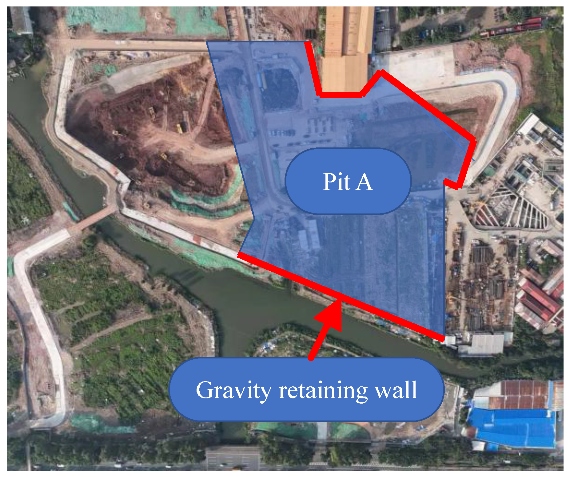
Figure 1. General layout plan of the foundation pit.
Buildings 15 04372 g001
Figure 2. Sectional view of foundation pit support.
Buildings 15 04372 g002
Figure 3. Foundation pit displacement monitoring. (a) Vertical displacement and (b) Lateral displacement.
Buildings 15 04372 g003
Figure 4. ML-based methodology for predicting foundation pit displacement.
Buildings 15 04372 g004
Figure 5. Prediction results of vertical displacement.
Buildings 15 04372 g005
Figure 6. Prediction accuracy of different models (vertical displacement).
Buildings 15 04372 g006
Figure 7. Vertical displacement prediction results using XGB.
Buildings 15 04372 g007
Figure 8. Fitting performance of horizontal displacement prediction.
Buildings 15 04372 g008
Figure 9. Prediction accuracy of different models (horizontal displacement).
Buildings 15 04372 g009
Figure 10. Horizontal displacement prediction results using ET.
Buildings 15 04372 g010
Figure 11. Vertical displacement prediction results (after SSA optimization).
Buildings 15 04372 g011
Figure 12. Prediction accuracy of different models after SSA optimization (vertical displacement).
Buildings 15 04372 g012
Figure 13. Vertical displacement prediction results using SSA-XGB.
Buildings 15 04372 g013
Figure 14. Fitting performance of horizontal displacement prediction (after SSA optimization).
Buildings 15 04372 g014
Figure 15. Prediction accuracy of different models after SSA optimization (horizontal displacement).
Buildings 15 04372 g015
Figure 16. Horizontal displacement prediction results using SSA-XGB.
Buildings 15 04372 g016
Figure 17. SHAP summary plot of feature impacts (vertical displacement).
Buildings 15 04372 g017
Figure 18. SHAP feature importance ranking (vertical displacement).
Buildings 15 04372 g018
Figure 19. SHAP summary plot of feature impacts (horizontal displacement).
Buildings 15 04372 g019
Figure 20. SHAP feature importance ranking (horizontal displacement).
Buildings 15 04372 g020
Table 1. Prediction errors of the vertical displacement test set.
DTRFETKNNXGBLGBM
R20.9480.7030.8490.9780.9880.972
RMSE1.6643.9642.8311.0780.7851.225
MAE1.4143.5262.4840.8590.5621.058
Table 2. Prediction errors of the horizontal displacement test set.
DTRFETKNNXGBLGBM
R20.9670.9640.9830.8960.9720.968
RMSE9.0509.3706.50816.0028.2398.941
MAE5.3356.9714.04614.7364.9868.022
Table 3. Core hyperparameters optimized for each model.
ModelParameter NameParameter MeaningValue
DTmax_depthmaximum tree depth8
min_samples_leafminimum number of samples per leaf2
min_samples_splitminimum samples to split a node4
RFn_estimatorsnumber of estimators200
max_depthmaximum tree depth10
min_samples_splitminimum number of samples to split a node4
ETn_estimatorsnumber of estimators250
max_depthmaximum tree depth12
min_samples_splitminimum number of samples to split a node10
KNNn_neighborsnumber of neighbors7
weightstype of weightsdistance
leaf_sizeleaf size of the tree30
XGBn_estimatorsnumber of estimators300
learning_ratelearning rate0.05
max_depthmaximum tree depth6
reg_lambdaL2 regularization1.0
LGBMn_estimatorsnumber of estimators1000
learning_ratelearning rate0.06
max_depthmaximum depth10
num_leavesnumber of leaves64
bagging_fractionsubsample rate per iteration0.9
lambda_l2L2 regularization1.0
Table 4. Prediction errors of the vertical displacement test set using SSA-XGB.
SSA-DTSSA-RFSSA-ETSSA-KNNSSA-XGBSSA-LGBM
R20.9740.9360.9660.9830.9880.982
RMSE1.1801.8361.3510.9530.7850.983
MAE0.9331.5761.1220.7280.5620.757
Table 5. Prediction errors of the horizontal displacement test set using SSA-XGB.
SSA-DTSSA-RFSSA-ETSSA-KNNSSA-XGBSSA-LGBM
R20.9730.9840.9690.9890.9900.986
RMSE8.1716.2138.7265.2945.6845.887
MAE3.9474.6236.5653.6382.4273.922
Disclaimer/Publisher’s Note: The statements, opinions and data contained in all publications are solely those of the individual author(s) and contributor(s) and not of MDPI and/or the editor(s). MDPI and/or the editor(s) disclaim responsibility for any injury to people or property resulting from any ideas, methods, instructions or products referred to in the content.