Research on Intelligent Identification Model of Cable Damage of Sea Crossing Cable-Stayed Bridge Based on Deep Learning

Abstract

To accurately evaluate the health condition of the cables of a cross-sea cable-stayed bridge under typhoon effects and to improve the efficiency of damage identification, an accurate bridge damage identification method combining convolutional neural network (CNN) and Bidirectional Long Short-Term Memory (BiLSTM) is proposed. A numerical model of the cable-stayed bridge was first established in ANSYS. Based on the monitoring data of Super Typhoon Mujigae, a three-dimensional fluctuating wind field was generated by harmonic synthesis. Through transient analysis, the static and dynamic responses of the cable-stayed bridge under typhoon loads were analyzed, and the critical cable locations most susceptible to damage were identified. Subsequently, the acceleration signals of the structural damage states under typhoon were extracted, and the damage-sensitive features were obtained through the Hilbert transform. Finally, an intelligent damage identification model for cable-stayed bridges was established by combining CNN and BiLSTM, and the identification results were compared with those obtained using CNN and BiLSTM individually. The results indicate that the neural network model combining CNN and BiLSTM performs significantly better than either CNN or BiLSTM alone in predicting both the location and degree of damage. Compared with the standalone CNN and BiLSTM models, the proposed hybrid CNN–BiLSTM network improves the accuracy of damage-location identification by 1.6% and 2.42%, respectively, and achieves an overall damage-degree identification accuracy exceeding 98%. The findings of this study provide theoretical and practical support for the intelligent operation and maintenance of cable-stayed bridges in coastal regions. The proposed approach is expected to serve as a valuable reference for evaluating large-span bridge structures under extreme wind conditions.

1. Introduction

Cable stays are critical load-bearing components in cable-stayed bridges, and their condition directly affects overall structural stability and safety. During long-term service, cables are subjected to combined effects of external loads, environmental corrosion, and extreme weather events such as typhoons. These factors may lead to material degradation and structural damage, thereby threatening the safe operation of bridges. Therefore, research on damage identification and timely health monitoring of stay cables is of great scientific and engineering significance.

Bridge damage identification is typically performed using static test data (e.g., stress, displacement) [1,2] and dynamic test data (e.g., frequency, mode shape) [3,4,5] to determine whether, where, and to what extent the structure has been damaged. In particular, dynamic fingerprint-based methods enable real-time monitoring and efficient detection, providing distinct advantages and widespread applicability [6]. Based on feature characteristics, dynamic fingerprints are generally categorized into four types: direct modal parameter-based features [7,8], modal parameter function-based features [9,10], curvature-based features [11,12], and non-modal vibration signal features [13,14,15]. Chang et al. [16] demonstrated through field tests on a steel truss bridge that multiple modal frequencies and Modal Assurance Criterion/Coordinate Modal Assurance Criterion (MAC/COMAC) values could effectively detect damage presence and severity. Mekjavi et al. [17] proposed a frequency-change-based method, and experiments on concrete and steel bridges confirmed its capability to locate and quantify damage even under stiffness degradation.

Traditional modal analysis-based approaches, however, have been shown to exhibit limited sensitivity to minor or localized damage and high susceptibility to noise and environmental variations, often leading to false or inaccurate results. To overcome these limitations, signal analysis techniques have been employed to extract damage-sensitive features from dynamic response data. For example, Mostafa et al. [18] used instantaneous frequency extracted by Wavelet Synchrosqueezed Transform (WSST) for vehicle–bridge interaction analysis, achieving higher accuracy than resonance frequency-based indicators. Ahmadi et al. [19] applied a Bern–Jordan time–frequency distribution with a novel damage index (C-index), enabling early-stage damage localization with high precision.

In recent years, deep learning techniques have been increasingly applied to bridge damage identification, as they can construct nonlinear mappings between damage-sensitive features and structural states. Convolutional neural networks (CNNs) have been widely adopted for damage classification and localization due to their effectiveness in vibration feature extraction [20,21,22,23]. To overcome the limitations of single-scale feature recognition, hybrid deep learning frameworks integrating CNNs and Long Short-Term Memory (LSTM) networks have been developed to capture both spatial and temporal features. Zhou et al. [24] compared four types of input features for CNN-based seismic damage identification. Fu et al. [25] utilized a CNN–LSTM framework, achieving 94% localization accuracy and 8.0% average relative error. Shan et al. [26] proposed a multi-scale CNN–LSTM model using improved modal decomposition and Hilbert transform, while Nguyen-Ngoc et al. [27] developed a 1D CNN–LSTM–SAX (Symbolic Aggregate approXimation) hybrid model to enhance temporal learning and improve recognition accuracy.

Conventional modal analysis is effective for global damage detection but exhibits limited sensitivity to early-stage or localized damage and is highly influenced by ambient temperature, traffic loads, and boundary condition variations. Signal-based methods, employing wavelet transform, Hilbert–Huang transform, and other time–frequency analysis tools, have enhanced the extraction of damage-sensitive features. However, their reliability still depends heavily on manually designed indicators and remains vulnerable to measurement noise and environmental interference. In contrast, deep learning techniques have demonstrated strong capability in capturing spatial–temporal features from structural responses, significantly improving the accuracy, automation, and adaptability of damage identification. Despite these advances, most studies have limited attention to cable-stayed bridges operating in extreme environments such as typhoons. To bridge these gaps, this study proposes an intelligent damage identification framework for stay cables under typhoon-induced excitations. In the proposed approach, instantaneous frequency features are extracted through the Hilbert–Huang transform (HHT) to capture damage-sensitive characteristics of the cable responses. These features are then combined with a neural network model to construct a nonlinear mapping between the dynamic behavior and damage states, enabling accurate, robust, and efficient identification of cable damage under complex aerodynamic and structural coupling conditions.

2. Structural Dynamic Response of Cable-Stayed Bridges Under Typhoon

2.1. Project Overview

The Zhanjiang Bay Bridge is a double tower double cable plane hybrid beam structure, using a five-span continuous semi-floating system with spans of 60 m, 120 m, 480 m, 120 m, and 60 m, respectively. The whole bridge is 840 m long. The main beam is a reinforced concrete structure. The main beam is a composite of steel and concrete, with concrete beams positioned at both ends of the span and a steel box beam in the middle. The cable bent tower is a reinforced concrete construction, with a height of 155.1 m above the supporting platform and 113.8 m above the bridge deck. The double cable surface fan-shaped arrangement in the cable space is made of low relaxation high-strength epoxy coated steel strands with a diameter of 15.24 mm, a strength of Ry = 1860 Mpa, and covered with HDPE protective layer. The horizontal spacing between the two cable surfaces on the bridge deck is 27.7 m, the cable spacing of the inclined cable on the longitudinal steel box beam is 16 m, and the cable spacing on the side span concrete beam section is 8 m. There are 112 cables for the whole bridge, with 56 cables on one side. The cable numbers are defined from east to west, with the left-side cables sequentially labeled J14 to J1 and S1 to S14 and the right-side cables labeled S′14′ to S1′ and J1′ to J14′. The cable-stayed bridge’s general layout is illustrated in Figure 1.

2.2. Model Building

Firstly, a 3D model of the cable-stayed bridge is created in ANSYS. The main beam, bridge tower, and piers are modeled using Beam4 spatial beam elements, and rigid arm extensions are used to connect the main beam to the cables. The cable is simulated using a rod element Link10, and the prestressing of the cable is achieved by setting the initial strain. The anchorage points of the diagonal cables are the natural nodes of the beam elements, and the beam element nodes and cable nodes are connected by rigid connecting rods. The upper dead load of the bridge is discretized into additional nodal masses on a finite number of nodes, the torsional stiffness of the main beam, bridge tower, and pier is simulated using the mass moment of inertia, and structural mass is applied on the nodes using mass element MASS21. The main tower is constructed from reinforced concrete, and the bridge tower is divided into 7 sections for simulation based on the bridge’s geometric data. The main beam, bridge tower, and piers are modeled with constraints that match the actual design of the bridge. The material parameters for each component are detailed in

Table 1. Material parameters of each part.

Structural Component	Material	Poisson’s Ratio	Density (kg/m3)	Elastic Modulus (Pa)
Steel box girder	Q345qc steel	0.3	7850	2.0 × 1011
Concrete main beam	C50 concrete	0.1667	2550	3.5 × 1010
Cable bent tower	C50 concrete	0.1667	2600	3.55 × 1010
Deck pavement	asphalt concrete	0.25	2300	1.5 × 109
Cable	Φ15.24 mm steel strand	0.3	7870	1.95 × 1011
Cable bent tower base, side piers, and auxiliary Pier Shaft	C40 concrete	0.2	2550	3.3 × 1010

and the finite element model is shown in Figure 2.

To validate the effectiveness of the finite element model, the bridge frequencies obtained from finite element calculations are compared with the experimentally measured frequencies [28], as shown in

Table 2. Comparison between calculated frequency and measured frequency of cable-stayed bridge.

Frequency/Hz
Serial No.	Measured Value	Calculated Value	Error	Mode Description
1	0.352	0.336	4.5%	first-order symmetrical vertical bend
2	0.3711	0.364	1.9%	first-order symmetrical horizontal bend
3	0.4490	0.452	0.6%	first-order antisymmetric vertical bend
4	0.6836	0.654	4.3%	first-order antisymmetric horizontal bend
5	1.0160	1.099	8.1%	main beam torsion

. It can be observed from Table 2 that the overall difference between the calculated and measured frequencies is relatively small. However, as the frequency order increases, the error between the structural frequencies of the computational model and the measured frequencies also increases. This discrepancy is primarily attributed to the fact that higher-order modes are associated with local vibrational characteristics of the structure, and the current model exhibits certain inaccuracies in simulating local details of the actual bridge. For vertical, lateral, and torsional directions, the errors between the calculated and measured values remain within an acceptable range. It can be concluded that the numerical model of the cable-stayed bridge established in this study is effective.

2.3. Dynamic Response Analysis of Cable-Stayed Bridge Under Typhoon

In the simulation process of fluctuating wind speed time histories, the components of cable-stayed bridges are first discretized, and wind loads are applied to each bridge node. When simulating spatially varying wind speeds, the wind field is modeled as a random vector process at discrete spatial locations, where the wind speed at each point comprises components in three directions: along-wind, across-wind, and vertical. Based on the structural characteristics of the cable-stayed bridges, the wind field is simplified into four independent one-dimensional multivariate random wind fields for simulation, including the transverse direction of the main girder, the vertical direction of the main girder, the transverse direction of the west tower, and the transverse direction of the east tower. The target wind spectrum models for wind field simulation employ the Kaimal spectrum and Panofsky spectrum recommended by specifications as the wind speed spectra at the bridge site. Based on the theory developed by Shinouzuka and Deodatis [18], transverse and vertical fluctuating wind speed time histories are generated for 58 simulation points acting on the main girder, while transverse fluctuating wind speed time histories are generated for 42 simulation points acting on the two bridge towers located on the east and west banks. Wind speed simulation points on the main beam are positioned at the anchorage locations between the cables and main girder, rather than being equally spaced. Wind speed simulation points on the bridge towers are distributed at equal 10 m intervals.

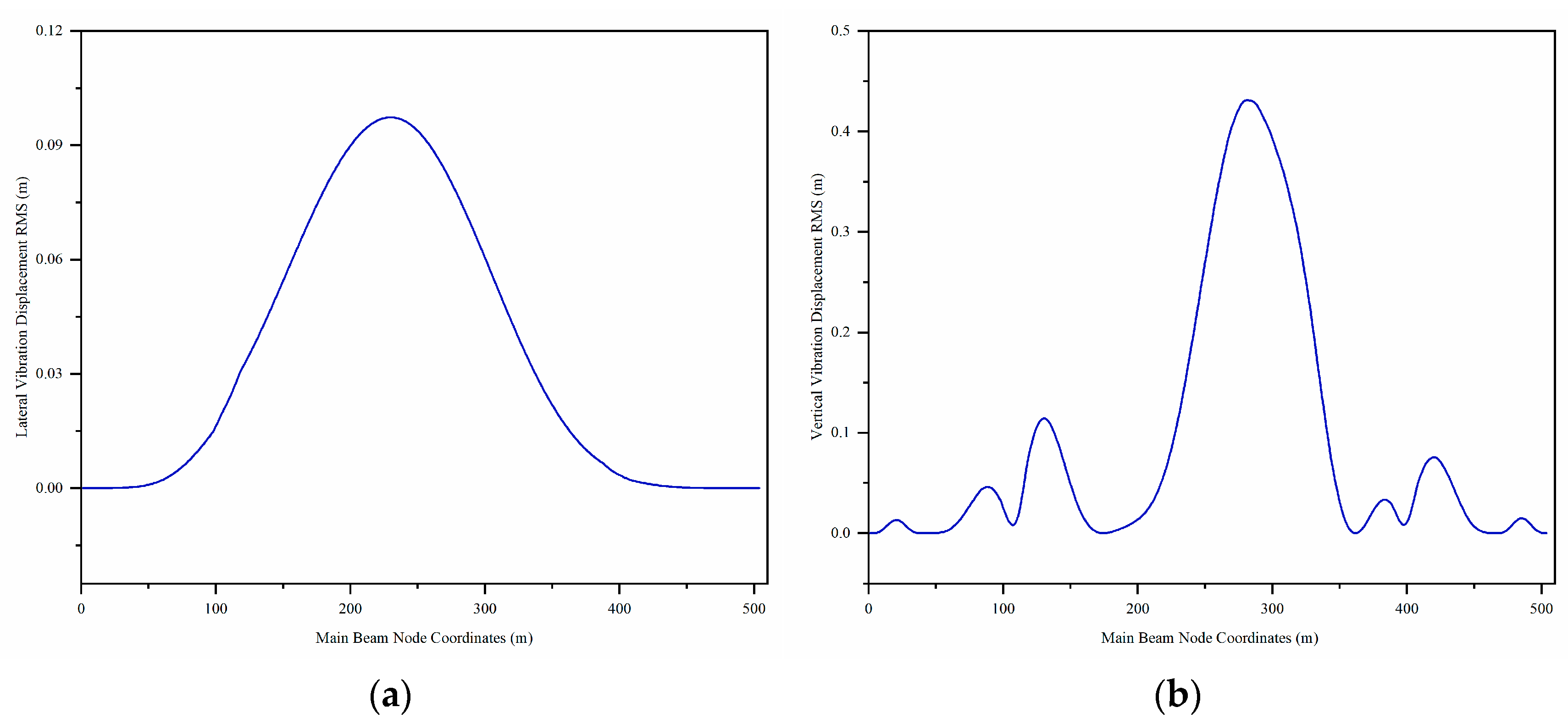
Based on meteorological observations and specialized wind studies, the average wind speed of Typhoon “Mujigae” at the site is 50 m/s. The bridge deck wind field is numerically simulated using MATLAB 2024, with a span of L = 840 m, beam height z = 50 m, ground roughness coefficient 0.12, and average wind speed at beam height U(z) = 50 m/s. In the simulation, all action points corresponded to finite element nodes, resulting in 158 wind speed time-history points. The converted buffeting force time histories and static wind loads are applied to the finite element model in ANSYS 2019 using transient dynamic analysis, yielding the bridge’s time-history response under typhoon. Displacements are generated in along-wind, cross-wind, and vertical directions. Root-mean-square (RMS) values of displacement are calculated for each node to quantitatively evaluate positional behavior. Figure 3 shows that RMS values of along-wind and vertical displacements along the main beam are approximately symmetric, decreasing from mid-span toward the supports. Peak RMS values occur at mid-span, indicating that the dynamic response is most pronounced in this region.

3. Introduction to Neural Networks

3.1. CNN

Deep learning is a machine learning approach inspired by biological neurons that mimics the neural network structure of the human brain to address complex problems. The essence of deep learning involves building network architectures with multiple layers of nonlinear processing units (neurons), which automatically extract features from raw data and facilitate learning. The deep learning model is illustrated in Figure 4.

Neural networks feature a multi-layered architecture consisting of input layers, hidden layers, and output layers, where each layer contains multiple neurons. Raw data is received by the input layer, features are extracted through the hidden layers, and prediction results are generated by the output layer. Computations are performed throughout the network using two trainable parameters: weights and biases. The training process is based on the backpropagation algorithm: forward propagation is first conducted to compute the output, the loss function is then employed to measure the error, gradients are subsequently calculated, and finally an optimizer (such as gradient descent or Adam) is used to update parameters for loss minimization. Common neural network architectures include CNN, recurrent neural networks (RNN), and Transformers (utilizing self-attention mechanisms). In this study, CNN, Bi-LSTM (a variant of RNN), and the combined CNN-BiLSTM architecture are adopted as damage identification models.

CNN represents a type of deep feedforward neural network that incorporates convolutional computations with deep hierarchical structures, serving as one of the fundamental algorithms in deep learning. Through its hierarchical architecture of convolutional layers, pooling layers, and fully connected layers, local features are automatically extracted from input data, information is progressively compressed, redundancy is reduced, and generalization capability is enhanced.

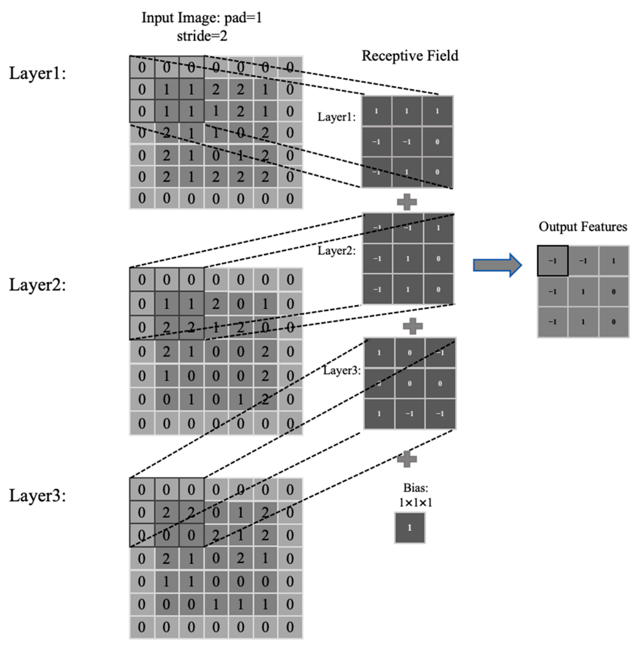
Convolutional layers are employed to extract local features from input data and comprise multiple convolutional kernels. Each kernel slides across the input data and performs convolution operations within corresponding regions to extract features. The operational process of convolutional kernels is shown in Figure 5. Parameters of convolutional layers include kernel size, stride, and padding, which collectively determine the dimensions of output feature maps produced by the convolutional layer. The expression is given as follows:

$$\mathrm{f}\left(\mathrm{x}\right)=\sum _{\mathrm{ij}}^{\mathrm{n}}{\mathsf{\theta }}_{\mathrm{ij}}·{\mathrm{x}}_{\mathrm{ij}}+\mathrm{b}$$

(1)

where f(x) represents the output feature value, denotes the weight value of the convolutional kernel at row i and column j, represents the input value at row i and column j, b is the bias term.

Since samples in actual training processes are often nonlinear while input features extracted through convolution operations remain linear, nonlinear activation functions are introduced to enhance model training effectiveness. Commonly employed activation functions include the Sigmoid function, tanh function, and ReLU function. The pooling layer functions to compress feature maps, extract primary features, and reduce the computational complexity of networks. Typical pooling approaches include average pooling and max pooling. Through pooling operations, feature maps can be sampled to decrease parameter quantities and enhance training efficiency. The fully connected layer is typically positioned at the end of convolutional neural networks and serves to map features extracted by preceding convolution and pooling layers to specific task outputs such as classification or regression. The formula can be expressed as follows:

$$\mathrm{f}\left(\mathrm{x}\right)=\mathrm{W}·\mathrm{x}+\mathrm{b}$$

(2)

where x is the input to the fully connected layer, W represents the weight matrix, and b denotes the bias term.

3.2. BiLSTM

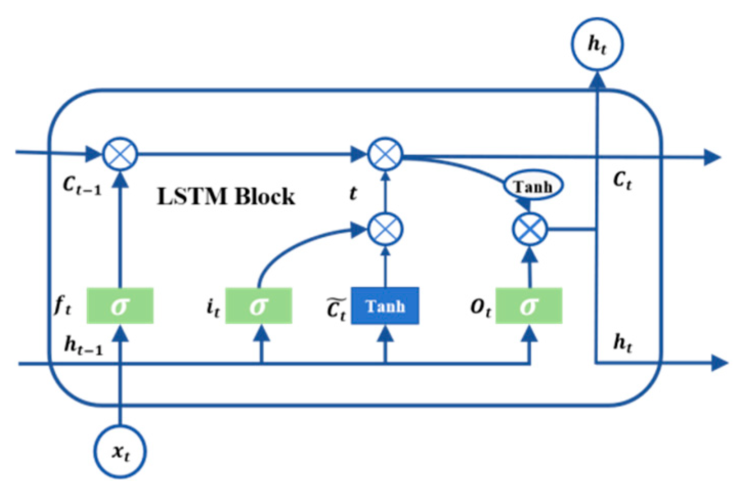
In 1997, LSTM was proposed by Hochreiter and Schmidhuber, addressing the long-term dependency issues inherent in RNNs through the incorporation of forget gates, input gates, and output gates. The architectural structure of the LSTM neural network model is illustrated in Figure 6.

Traditional LSTM networks can only utilize historical information, which may limit their feature extraction capabilities and subsequently affect prediction accuracy. BiLSTM effectively combines past and future information by simultaneously training both forward and backward LSTM units, thereby enhancing feature extraction while avoiding issues such as gradient vanishing or gradient explosion.

(1)

The forget gate controls the proportion of information retained from the previous memory cell state. This gate is updated by combining the output from the preceding time step with the current input through a sigmoid function.

$${\mathrm{f}}_{\mathrm{t}}=\mathsf{\sigma }({\mathrm{w}}_{\mathrm{f}}·\left[{\mathrm{h}}_{\mathrm{t}-1},\mathrm{x}\right]+{\mathrm{b}}_{\mathrm{f}})$$

(3)

(2)

The input gate controls the input to the cell state at the current time step, filtering out irrelevant and redundant information. The output from the first component of the input gate at time t determines what proportion of new information should be written into the memory cell state: the candidate and current memory cell states are represented, respectively.

$$i_t=\sigma (w_i·\left[h_{t-1},x_t\right]+b_i)$$

(4)

$$\widetilde{C_t}=tan\mathrm{h}(w_c·\left[h_{t-1},x_t\right]+b_c)$$

(5)

$$C_t=f_t·C_{t-1}+i_i·\widetilde{C_t}$$

(6)

(3)

The output gate determines how much information from the memory cell gets transmitted to the hidden state. After being filtered through the forget gate and input gate, the output signal state is selectively determined. The resulting hidden state represents the current time step, serving both as the LSTM’s output and as input for the subsequent time step.

$$o_t=\sigma (w_o·\left[h_{t-1},x_t\right]+b_o)$$

(7)

$$h_t=o_t·tan\mathrm{h}(C_t)$$

(8)

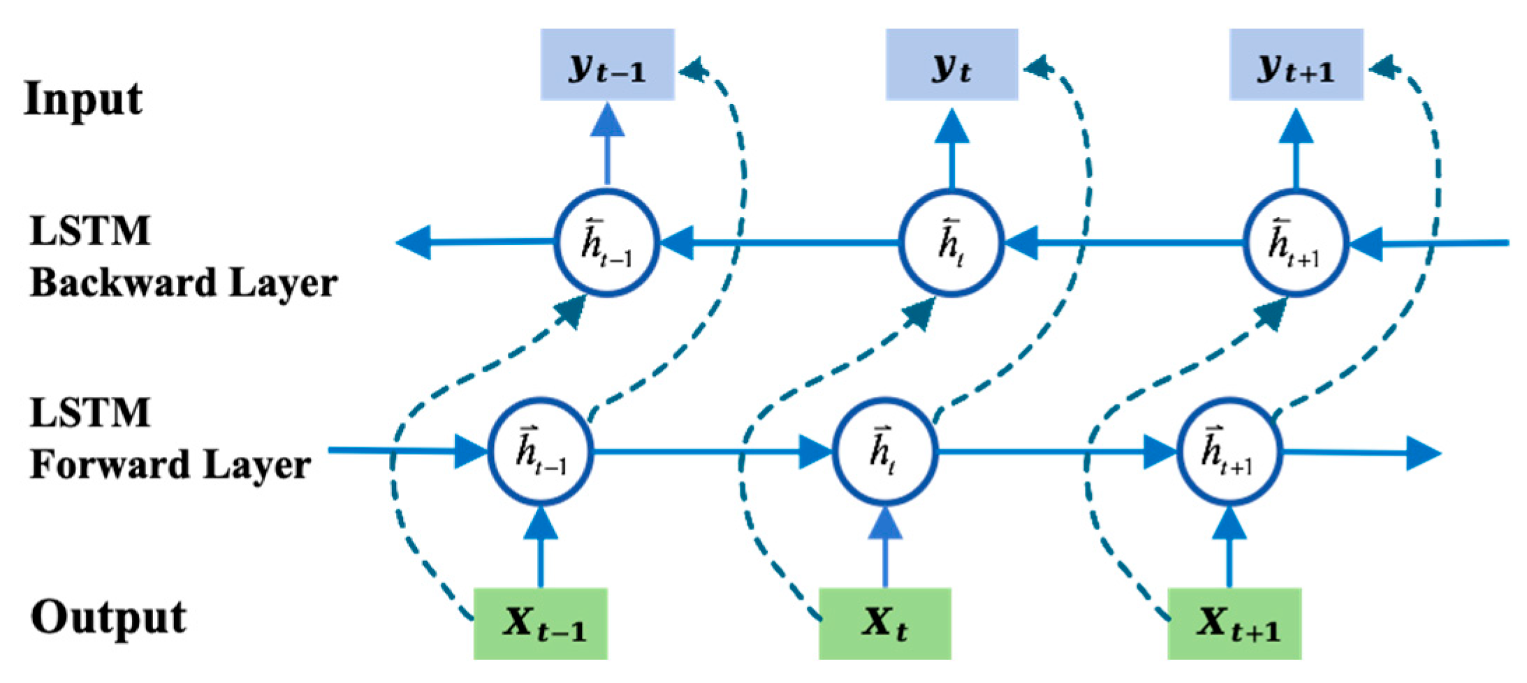
BiLSTM consists of layers operating in two transmission directions: a forward layer that processes information sequentially along the time series, and a backward layer that processes information in reverse chronological order. This architecture enables comprehensive extraction of both historical and future contextual information from time series data. The structure is illustrated in Figure 7. The forward layer processes the sequence chronologically to encode historical information, while the backward layer processes the sequence in reverse to encode future information. The output layer combines the bidirectional hidden states to produce the final output, with the mathematical expression given as follows:

$${\overrightarrow{h}}_t=LSTM(x_t,{\overrightarrow{h}}_{t-1})$$

(9)

$${\overleftarrow{h}}_t=LSTM(x_t,{\overleftarrow{h}}_{t-1})$$

(10)

$$y_t=\overrightarrow{W}{\overrightarrow{h}}_t+\overleftarrow{W}{\overleftarrow{h}}_t+b_y$$

(11)

3.3. CNN-BiLSTM

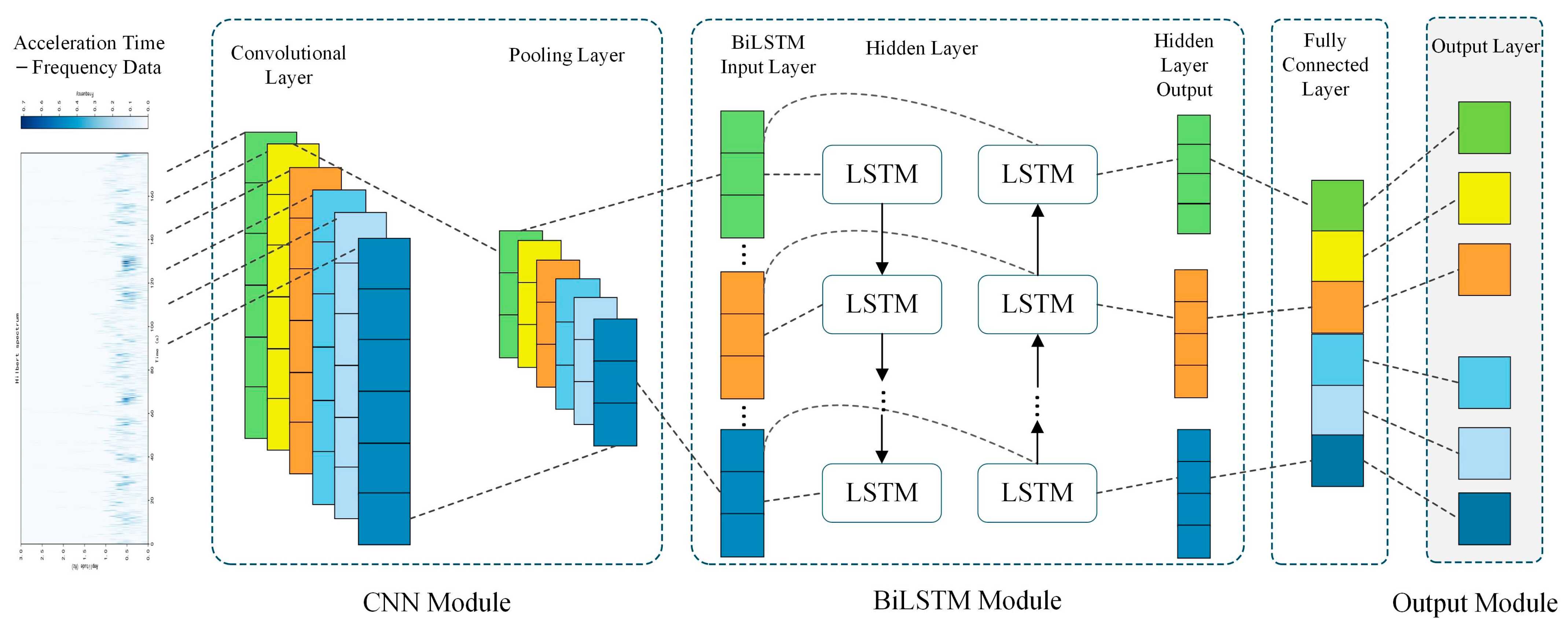
Single-scale feature extraction methods often exhibit limitations in accurately identifying structural damage. To improve identification accuracy and robustness, a hybrid convolutional neural network–bidirectional long short-term memory (CNN–BiLSTM) model is developed to identify cable damage in cable-stayed bridges under typhoon-induced dynamic loading. This hybrid framework combines the strengths of both architectures: the CNN component excels at local feature extraction and spatial pattern recognition, while the BiLSTM component is specialized in capturing temporal dependencies and dynamic sequential information.

Input layer: for the i-th cable damage scenario, the response indicators from all measurement points of the structure are treated as a time-dependent multivariate sequence $f(x_1,x_{21},\text{…},x_n,t)$. Before feeding the data into the prediction model, normalization is applied to eliminate magnitude differences among samples and enhance training stability.

Feature-extraction layer (CNN part): the CNN module employs two-dimensional convolutional kernels that slide over the input data to extract local temporal–spatial patterns of structural responses. Through successive convolution and max-pooling operations, the CNN transforms the raw acceleration data into high-dimensional feature maps that represent damage-sensitive characteristics. The convolution kernels effectively capture local disturbances and pattern variations in the signals, yielding robust feature sequences that characterize the nonlinear vibration behavior of stay cables.

Temporal-modeling layer (BiLSTM part): the feature matrices generated by the CNN are then passed to the BiLSTM network for sequential modeling. The BiLSTM processes the feature sequences in both forward and backward directions, thereby integrating past and future temporal information. This bidirectional transmission mechanism enables the model to capture long-term dependencies and contextual correlations within non-stationary vibration signals, significantly enhancing its capability to describe the continuous and temporally dependent dynamic responses of stay cables under typhoon excitation.

Output layer: the output from the BiLSTM is fed through fully connected layers to produce the final prediction vector representing the damage-degree factors for each structural element. For instance, when Cable 14 experiences 10% damage, the output vector becomes (0, 0, 0, …, 0.1), where 0 denotes undamaged elements and 0.1 represents the corresponding damage degree factor. The final regression or classification layer determines both the location and severity of structural damage.

Through the synergistic combination of CNN-based spatial feature extraction and BiLSTM-based temporal dependency modeling, the CNN–BiLSTM framework fully exploits potential features of acceleration signals in both the time-frequency and time-series domains, thereby achieving accurate and reliable identification of cable damage states in cable-stayed bridges. The process flow of this identification method is illustrated in Figure 8.

4. Train the Model Based on the Damage Sample Library

4.1. Construction of Damage Sample Library

Due to the symmetrical distribution of geometric information of cable-stayed bridge, the east bank side of cable-stayed bridge is selected for analysis in this paper. The locations of cables most vulnerable to damage under typhoon are determined through analysis of main beam displacement and cable stress variations. A numerical simulation is conducted using a time step of 0.1 s for 600 s time history analysis, yielding 6000 sets of time history data for each cable. The root-mean-square (RMS) values of each cable force are calculated based on the 6000 sets of cable force data, as presented in Figure 9. Figure 9a reveals that the RMS of cable stress exhibits a positive correlation with the RMS of main beam-anchorage node displacement. The bank of the cable-stayed bridge is divided into three areas (R1, R2, R3) by three piers. It can be seen from Figure 9b that under the typhoon, in R3 area, the main beam has a large displacement in the middle of the span, and the stress amplitude of the cables (S14, S13 and S12) near the middle of the span is greater than that of other locations. In this area, cables S14, S13 and S12 are more prone to damage. In R2 area, the displacement at the main beam node 87–97 (corresponding to the cable numbers J1 and J2) is locally the largest, and the stress amplitude of the cable is also relatively large in this area, where the cables J1 and J2 are more prone to damage. In R1 area, due to the influence of support constraints, the displacement in this area is small. So, it is mainly analyzed from the change in stress. In this area, the stress changes evenly, and the longest side span cable J14 changes the most, in R1 area, cable J14 is the most vulnerable to damage. Through analysis of main beam displacement and cable stress changes, this paper determines that the six cables that are most prone to damage under the typhoon load are S14, S13 and S12 in R3 area, J2 and J1 in R2 area, and J14 in R1 area.

Damage is simulated by reducing the elastic modulus of the cables, with damage severity classified into six levels: undamaged, 10%, 20%, 30%, 40%, and 50%. The damage configurations are established as single damage and double damage scenarios. Under typhoon conditions with wind speeds of 50 m/s, acceleration response signals are extracted from the anchorage nodes connecting six vulnerable cables to the main beam. For each working condition, 300 s samples are collected using an integration time step of 0.1 s, resulting in 10 data points per second. A total of 406 vertical acceleration response data points are obtained as the initial dataset. Figure 10 presents the acceleration time history responses for cable S14 under both undamaged conditions and 50% damage severity. As shown in Figure 10, the acceleration response signals demonstrate minimal variation between damaged and undamaged states, which complicates the extraction of damage characteristics for certain cables. Additionally, the vibration response signals exhibit pronounced non-stationary behavior, necessitating enhanced decomposition accuracy of structural dynamic response signals to identify features with greater sensitivity to bridge damage.

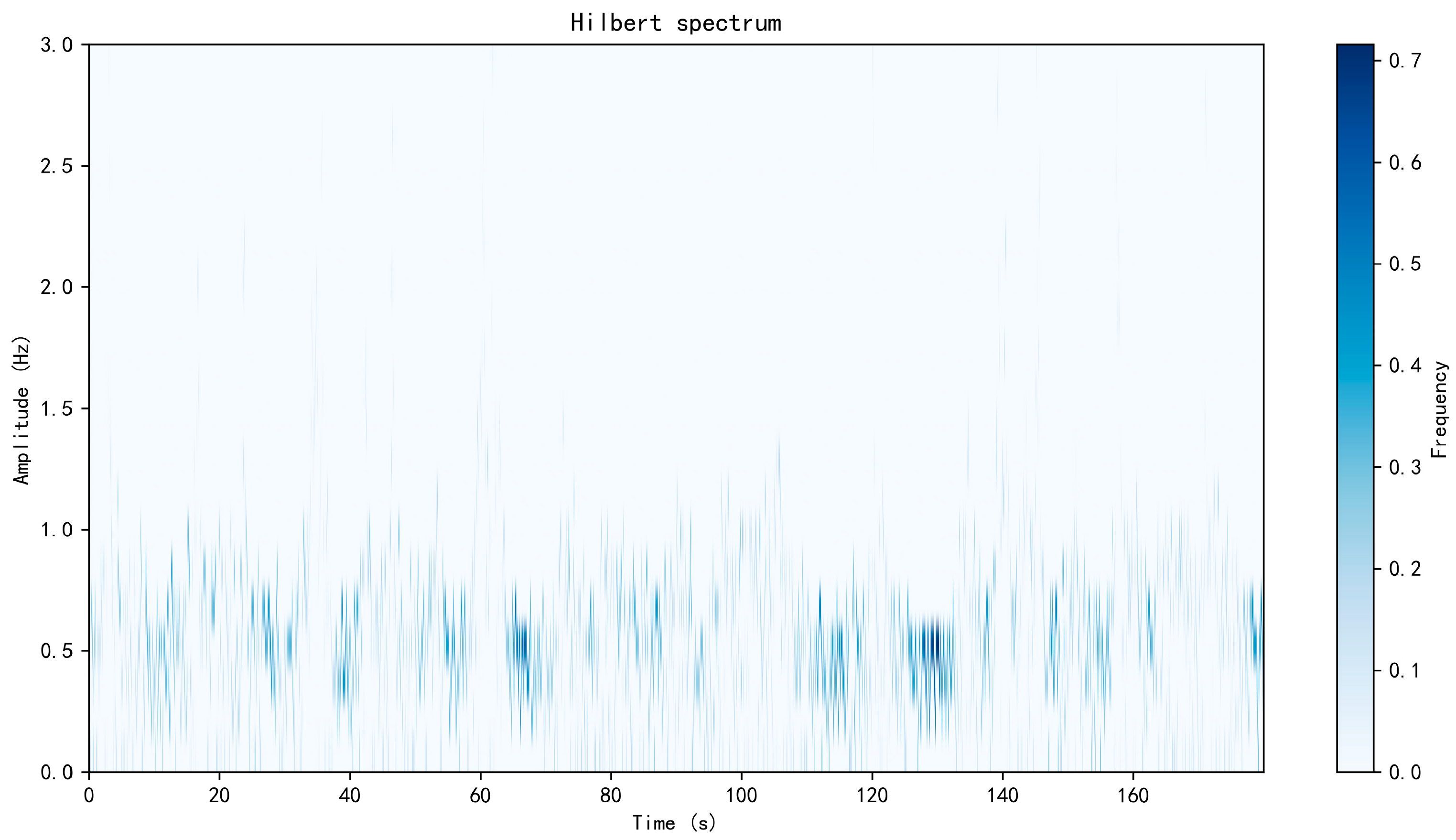
The Hilbert time–frequency spectrum reveals the relationship between signal time, instantaneous frequency, and amplitude, showing how signal amplitude changes with frequency across the entire frequency range. When structural damage develops, vibration signal variations are reflected in the time–frequency plane. The Hilbert transform effectively addresses the challenge of extracting damage-sensitive features from signals in both time and frequency domains encountered in conventional damage diagnosis. Therefore, this study employs the Hilbert transform to extract sensitive features from acceleration signals. Using the vertical acceleration at measuring point S14 of the cable-stayed bridges cable under typhoon conditions with 0° wind attack angle as an example, Python 3.13 programming is applied to perform the Hilbert transform, yielding two time-varying vectors—instantaneous frequency and instantaneous energy rate—along with characteristic parameters including the Hilbert time–frequency spectrum. The frequency spectrum of cable S14 is generated through the Hilbert transform, as presented in Figure 11. The amplitude distribution of the Hilbert time–frequency spectrum across the time–frequency plane reveals changes in the dynamic response characteristics of cable stays under various structural conditions, allowing the neural network to capture distinctive data patterns associated with different structural states.

Acceleration signal data are extracted from the dynamic response of cable-to-main beam anchorage node structures and divided into training and testing sets at an 8:2 ratio. The Hilbert transform is employed to convert one-dimensional vibration signals into two-dimensional time-frequency images. The output dimensions are adjusted and damage category labels are assigned to facilitate subsequent training and testing procedures. Data preprocessing and model training are performed sequentially following these steps:

(1)

Normalization is applied to the sample database to eliminate dimensional differences and enhance training convergence efficiency.

(2)

The normalized training set is fed into the neural network to conduct model training and cross-validation.

(3)

SmoothL1Loss is chosen as the loss function during training to achieve a balance between regression accuracy and stability.

(4)

Steps (2) and (3) are repeated until the predetermined number of training epochs is achieved, at which point the training process is concluded.

4.2. CNN Model Training Results

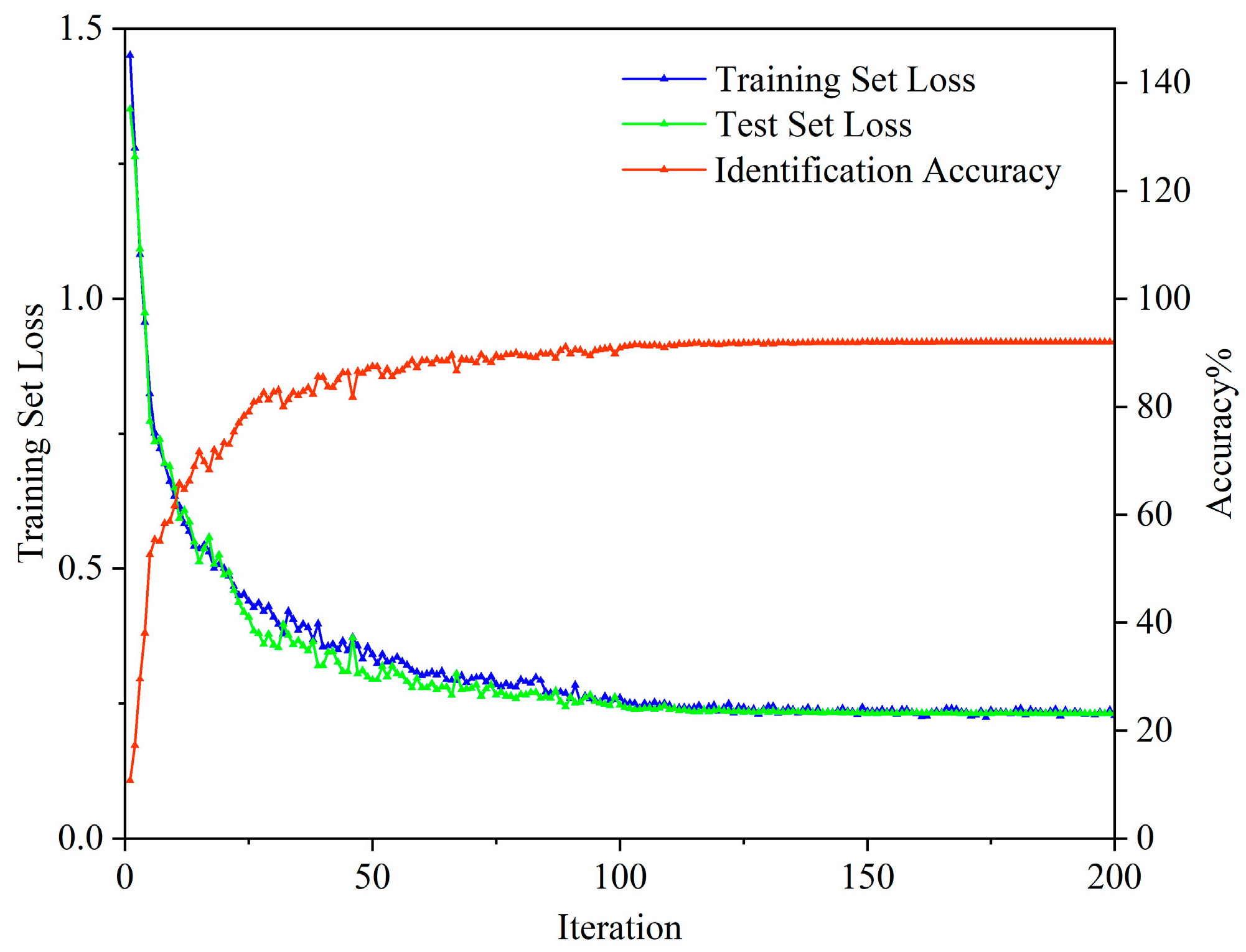
In the CNN model, The input tensor x has dimensions of 1799 × 406 × 6, where 1799 represents the time steps, 406 denotes the number of samples, and 6 corresponds to the number of monitored cable locations. The output tensor y has dimensions of 406 × 6, representing the predicted damage degree factors for the six target cables. The convolutional part of the network consists of a single convolution layer with a kernel size of 3, stride of 3, and padding of 1. The Rectified Linear Unit (ReLU) activation function is adopted to introduce nonlinearity and prevent gradient vanishing. A max-pooling layer is applied to downsample the feature maps with a pooling window of 2 × 2 and a stride of 2, effectively reducing computational complexity while retaining the most representative features. An initial learning rate of 0.001 is adopted, combined with the Adam optimizer’s dynamic learning rate optimization strategy, which enhanced training stability and prevented gradient oscillation during early training stages. The hyperparameters of the CNN model are shown in

Table 3. The hyperparameters of the CNN model.

Layer	Parameter Description	Value
Input layer	Input tensor dimension	1799 × 406 × 6
Output layer	Output tensor dimension	406 × 6
Convolution layer	Kernel size/Stride/Padding	3/3/1
	Activation function	ReLU
Fully connected layers	FC1: Input → Output	256 × 112 → 512
	FC2: Input → Output	512 → 256
	FC3: Input → Output	256 → 6
Loss function	-	Smooth L1 Loss
Learning rate	-	0.001–0.0005

.

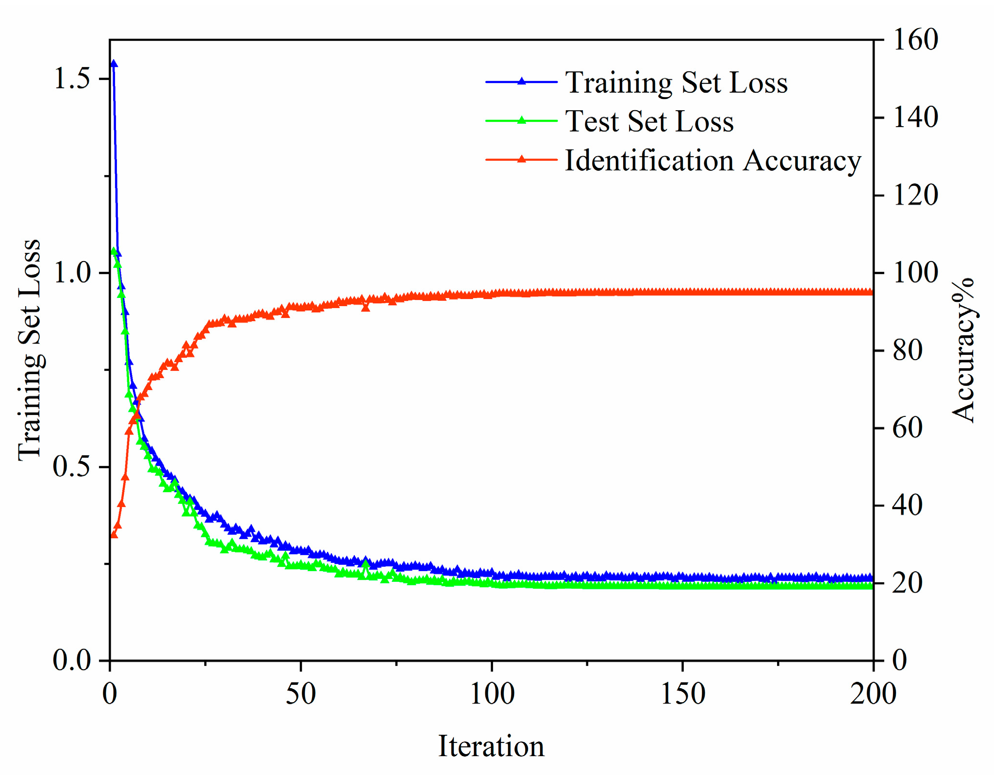
At the data level, 324 randomly selected damage conditions from 406 available damage scenarios were fed into the model, comprising a total of 538,200 damage data points. Following 100 training iterations, the loss function stabilized, indicating that the model had reached convergence. Following the completion of 200 training epochs, a prediction accuracy of 92% is achieved by the model on the independent test set. The accuracy curves for damage identification and loss values during the training and validation phases are presented in Figure 12.

4.3. BiLSTM Model Training Results

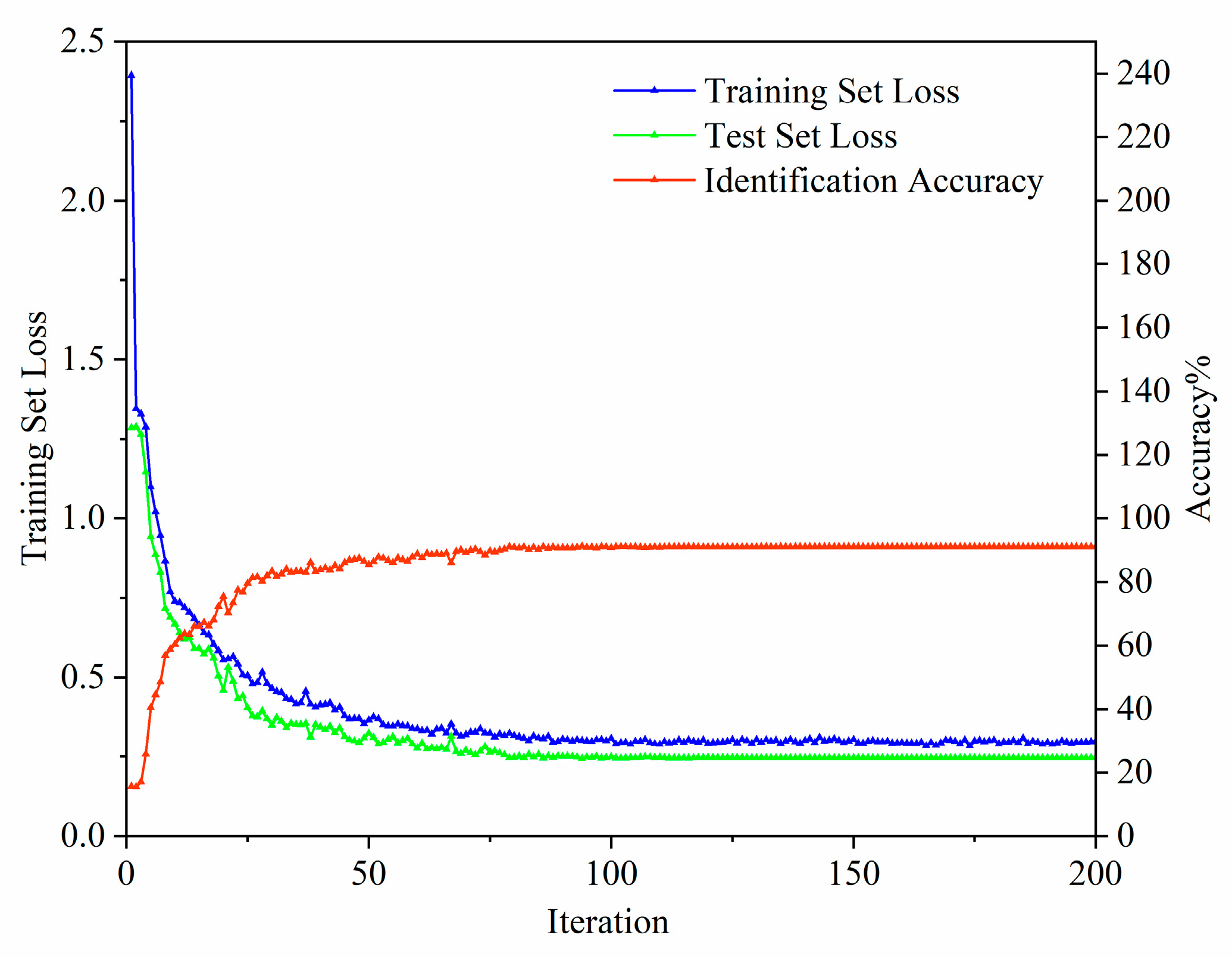
The BiLSTM model architecture consists of an input layer, two bidirectional LSTM layers, a fully connected layer, a softmax layer, and a final classification layer. The input layer dimension is defined as 6, corresponding to the number of monitored cable features. Each BiLSTM layer is composed of 256 hidden neurons, and two such layers are stacked to enhance the depth of feature extraction and representation capability. The Sigmoid and tanh activation functions are alternately applied to regulate nonlinear transformations and to prevent gradient vanishing. The outputs from the BiLSTM layers are transmitted to a fully connected layer for feature mapping, followed by a softmax layer that generates probability distributions for each operating condition. The final classification layer provides the corresponding damage state for each sample. The Smooth L1 Loss function is employed to improve robustness against outliers, and the learning rate is maintained consistent with that of the CNN model, decreasing adaptively from 0.001 to 0.0005. The model is trained for 200 epochs to ensure a fair comparison with the CNN and CNN–BiLSTM networks under identical optimization conditions. The hyperparameters of the BiLSTM model are shown in

Table 4. The hyperparameters of the BiLSTM model.

Layer	Parameter Description	Value
Input layer	Input dimension	6
Output layer	Number of BiLSTM layers	2
Hidden layers	Hidden units per layer	256
	Activation function	Sigmoid/tanh
Fully connected layers	Feature mapping to output	256 → 6
Loss function	-	Smooth L1 Loss
Learning rate	-	0.001–0.0005

.

Training results demonstrated that the BiLSTM model achieved approximately 92.9% prediction accuracy on the test set. The damage identification accuracy and loss value curves of the BiLSTM model during the training and validation processes are presented in Figure 13.

4.4. The Training Results of the Hybrid CNN-BiLSTM Model

A hybrid CNN–BiLSTM model is developed by integrating the spatial feature extraction capability of CNN with the temporal sequence learning advantage of BiLSTM. The front-end consists of three convolutional layers, and the back-end incorporates two bidirectional BiLSTM layers to capture temporal dependencies in the extracted feature sequences. The input feature space is constructed from the Hilbert-transformed time–frequency features derived from the acceleration responses of six monitored cable anchorage nodes. The corresponding input tensor has dimensions of 1799 × 406 × 6, representing time steps, sample number, and monitored cables, respectively. In the CNN component, 32 convolutional filters (kernel size = 3, stride = 3, padding = 1) are used, followed by ReLU activation and a 2 × 2 max-pooling layer for dimensionality reduction. The extracted spatial features are flattened and passed to the BiLSTM layers, each containing 256 hidden units, where bidirectional temporal dependencies are modeled. The output layer maps the learned temporal features to a six-dimensional vector corresponding to the damage-degree factors of the six target cables. The model is trained using Smooth L1 Loss and optimized by the Adam algorithm with a learning rate ranging from 0.001 to 0.0005. This configuration enables the model to achieve early convergence at approximately the 80th training epoch while improving accuracy to around 95%. The damage identification accuracy and loss values throughout the training process are presented in Figure 14.

4.5. Comparison and Analysis of Results

After training completion, a confusion matrix is employed to statistically analyze 492 predicted values from 82 damage conditions in the test set, with the resulting confusion matrix presented in Figure 15. Performance indicators for each neural network are calculated and are shown in

Table 5. Performance indexes of structural damage identification model.

Model	Accuracy (%)	Precision (%)	Recall (%)	F1 Score (%)
CNN	95.77	92.55	94.30	93.42
BiLSTM	94.96	92.9	91.14	92.01
CNN-BiLSTM	97.38	95.57	96.18	95.87

. Figure 15 reveals that CNN, BiLSTM, and the combined CNN-BiLSTM exhibit different recognition accuracies. Specifically, CNN misclassified 21 data samples, while BiLSTM misclassified 26 data samples, demonstrating relatively low recognition accuracy. The combined CNN-BiLSTM model misclassified only 13 data samples, showing recognition errors significantly lower than those of the individual CNN or BiLSTM models.

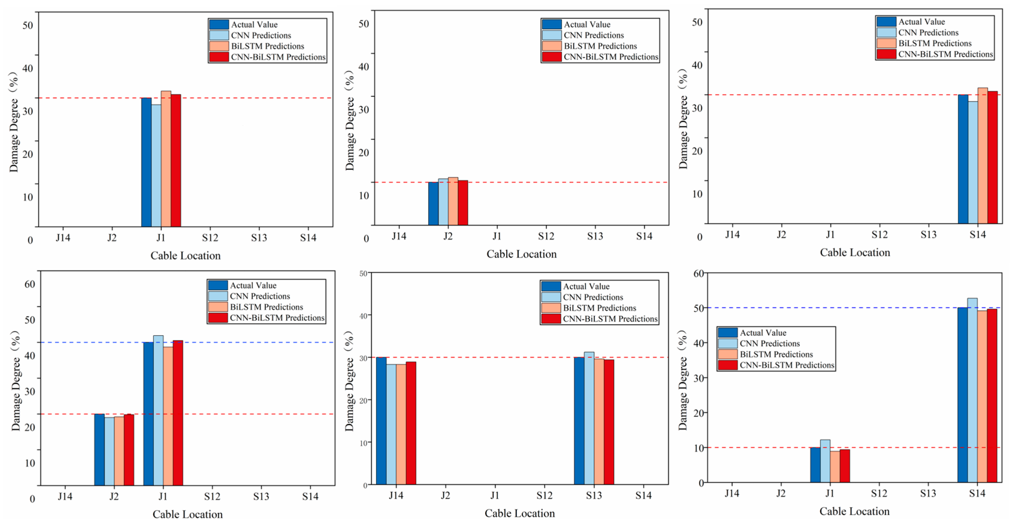
The results indicate that the CNN model achieved 95.77% accuracy for damage location identification, while the BiLSTM model achieved 94.96% accuracy for damage location identification. The combined CNN-BiLSTM model demonstrated superior performance with 97.38% accuracy for damage location identification. The proposed model achieves higher accuracy for damage location identification compared to the other two models. Based on the accuracy rates and confusion matrix results, the combined CNN-BiLSTM neural network model shows superior performance in predicting damage locations compared to individual CNN or BiLSTM models, while also providing relatively precise assessments of damage severity in affected cables. Analysis of the test dataset revealed that cases where damage locations are not identified were primarily concentrated under 10% damage conditions, with the maximum damage degree for cables incorrectly classified as undamaged reaching 13%. Figure 16 presents the recognition accuracy of three neural network models across different damage degree. The results demonstrate that the combined CNN-BiLSTM model exhibits superior recognition accuracy for both single and double damage scenarios when compared to standalone CNN or BiLSTM models.

Due to the uncertainty of wind-induced vibrations and interference from environmental noise, the model has a small probability of misjudgment. However, when compared with traditional methods, the model still demonstrates the advantages of being fast, efficient, and highly sensitive to minor damage. Therefore, it can be concluded that this approach can serve as an intelligent and effective method for diagnosing cable damage in cross-sea cable-stayed bridges.

5. Conclusions

Based on acceleration data obtained from a finite element model of cable-stayed bridges subjected to typhoon loading, a deep-learning-based framework combining CNN and bidirectional BiLSTM is developed to identify cable damage in a large-span cable-stayed bridge under typhoon-induced excitation. The main conclusions of this study are as follows:

(1)

Under typhoon loading, greater dynamic responses are observed in the cables located at the mid-span and side-span of the bridge, and these cables are therefore considered more prone to damage.

(2)

Damage-sensitive features such as instantaneous frequency and energy are effectively extracted from acceleration signals through the Hilbert transform. These parameters are found to capture the nonlinear and non-stationary characteristics of vibration responses under strong wind excitations, providing a more reliable basis for subsequent damage identification.

(3)

A structural damage identification approach combining CNN and BiLSTM networks is proposed. The combined neural network is shown to achieve an average accuracy of 92.01% for damage location identification across various working conditions, representing improvements of 1.6% and 2.42% compared with standalone CNN and BiLSTM networks, respectively. The average accuracy for damage degree identification under different conditions exceeds 98%. Therefore, the CNN–BiLSTM-based method is considered to significantly enhance the effectiveness of structural damage detection.

This study is conducted by integrating physical simulation, time–frequency analysis, and hybrid deep learning to improve the precision, reliability, and applicability of bridge health monitoring in marine environments. The findings are expected to provide valuable insights for real-time structural health monitoring, intelligent operation, and preventive maintenance under extreme wind conditions. However, this study has certain limitations. The present findings are based on a numerical model under a fixed 0° wind attack angle, and certain practical aspects, such as varying wind directions, environmental noise, and measurement uncertainty, were not fully encompassed. To address these aspects and enhance the model’s practical readiness, future work will systematically investigate its performance across a range of wind attack angles. We will also incorporate measured field data, explore transfer learning to improve model adaptability to real-world conditions, and pursue integration with real-time monitoring systems for continuous condition assessment.

References

1. Hua, X.G.; Ni, Y.Q.; Chen, Z.Q.; Ko, J.M. Structural Damage Detection of Cable-Stayed Bridges Using Changes in Cable Forces and Model Updating. J. Struct. Eng. 2009, 135, 1093–1106. [Google Scholar] [CrossRef]
2. Song, J.; Gu, C.; Su, H.; Gu, H.; Huang, X. Observed displacement data-based identification method of structural damage in concrete dam. Eng. Fail. Anal. 2016, 66, 202–211. [Google Scholar] [CrossRef]
3. Farahani, R.V.; Penumadu, D. Damage identification of a full-scale five-girder bridge using time-series analysis of vibration data. Eng. Struct. 2016, 115, 129–139. [Google Scholar] [CrossRef]
4. Zhang, Y.; Zhu, J. Damage identification for bridge structures based on correlation of the bridge dynamic responses under vehicle load. Structures 2021, 33, 68–76. [Google Scholar] [CrossRef]
5. Sarwar, M.Z.; Cantero, D. Deep autoencoder architecture for bridge damage assessment using responses from several vehicles. Eng. Struct. 2021, 246, 113064. [Google Scholar] [CrossRef]
6. Feng, D.M.; Feng, M.Q. Computer vision for SHM of civil infrastructure: From dynamic response measurement to damage detection-A review. Eng. Struct. 2018, 156, 105–117. [Google Scholar] [CrossRef]
7. Zhang, Y.; Tan, X.; Li, G.; Dong, J.; Guo, J.; Liu, F. Bridge Structure Damage Identification Based on Dynamic Characteristics. Coatings 2022, 12, 313. [Google Scholar] [CrossRef]
8. Abedin, M.; Mehrabi, A.B. Bridge damage identification through frequency changes. In Proceedings of the Sensors and Smart Structures Technologies for Civil, Mechanical, and Aerospace Systems 2021, Online, 22–27 March 2021. [Google Scholar]
9. Nick, H.; Aziminejad, A.; Hosseini, M.H.; Laknejadi, K. Damage identification in steel girder bridges using modal strain energy-based damage index method and artificial neural network. Eng. Fail. Anal. 2021, 119, 105010. [Google Scholar] [CrossRef]
10. Zhan, P.; Qin, X.; Zhang, Q.; Sun, Y. Damage identification in beam-like structure using strain FRF-based damage index and artificial neural network. Mech. Adv. Mater. Struct. 2023, 30, 2458–2476. [Google Scholar] [CrossRef]
11. He, M.; Yang, T.; Du, Y. Nondestructive identification of composite beams damage based on the curvature mode difference. Compos. Struct. 2017, 176, 178–186. [Google Scholar] [CrossRef]
12. Nguyen, D.H.; Wahab, M.A. Damage detection in slab structures based on two-dimensional curvature mode shape method and Faster R-CNN. Adv. Eng. Softw. 2023, 176, 103371. [Google Scholar] [CrossRef]
13. Wu, J.; Li, H.; Ye, F.; Ma, K. Damage identification of bridge structure based on frequency domain decomposition and strain mode. J. Vibroeng. 2019, 21, 2096–2105. [Google Scholar] [CrossRef]
14. Shandiz, S.K. Application of variational mode decomposition in vibration-based bridge damage detection. Proc. Inst. Civ. Eng. —Bridge Eng. 2024, 178, 277–299. [Google Scholar] [CrossRef]
15. Ahmadi, H.R.; Mahdavi, N.; Bayat, M. A novel damage identification method based on short time Fourier transform and a new efficient index. Structures 2021, 33, 3605–3614. [Google Scholar] [CrossRef]
16. Chang, K.C.; Kim, C.W. Modal-parameter identification and vibration-based damage detection of a damaged steel truss bridge. Eng. Struct. 2016, 122, 156–173. [Google Scholar] [CrossRef]
17. Mekjavi, I.; Damjanovi, D. Damage Assessment in Bridges Based on Measured Natural Frequencies. Int. J. Struct. Stab. Dyn. 2016, 17, 1750022. [Google Scholar] [CrossRef]
18. Mostafa, N.; Di Maio, D.; Loendersloot, R.; Tinga, T. Railway bridge damage detection based on extraction of instantaneous frequency by Wavelet Synchrosqueezed Transform. Adv. Bridg. Eng. 2022, 3, 12. [Google Scholar] [CrossRef]
19. Ahmadi, H.R.; Momeni, K.; Jasemnejad, Y. A new algorithm and damage index for detection damage in steel girders of bridge decks using time-frequency domain and matching methods. Structures 2024, 61, 106035. [Google Scholar] [CrossRef]
20. He, H.-x.; Zheng, J.-c.; Liao, L.-c.; Chen, Y.-j. Damage identification based on convolutional neural network and recurrence graph for beam bridge. Struct. Health Monit. 2020, 20, 1392–1408. [Google Scholar] [CrossRef]
21. Yang, S.; Huang, Y. Damage identification method of prestressed concrete beam bridge based on convolutional neural network. Neural Comput. Appl. 2021, 33, 535–545. [Google Scholar] [CrossRef]
22. Wang, C.; Ansari, F.; Wu, B.; Li, S.; Morgese, M.; Zhou, J. LSTM approach for condition assessment of suspension bridges based on time-series deflection and temperature data. Adv. Struct. Eng. 2022, 25, 3450–3463. [Google Scholar] [CrossRef]
23. Yin, X.; Yang, Y.; Huang, Z.; Yan, W. Bridge Damage Identification Based on LSTM Network and Contact Point Response. Int. J. Struct. Stab. Dyn. 2025, 25, 2450268. [Google Scholar] [CrossRef]
24. Zhou, X.; Zhao, Y.; Khan, I.; Cao, L. Comparative Study on CNN-based Bridge Seismic Damage Identification Using Various Features. KSCE J. Civ. Eng. 2024, 28, 5618–5627. [Google Scholar] [CrossRef]
25. Fu, L.; Tang, Q.; Gao, P.; Xin, J.; Zhou, J. Damage Identification of Long-Span Bridges Using the Hybrid of Convolutional Neural Network and Long Short-Term Memory Network. Algorithms 2021, 14, 180. [Google Scholar] [CrossRef]
26. Shan, D.; Sun, R.; Tan, K. Damage identification for Cable-Stayed model bridges on shaking Table based on joint CNN & LSTM with Multi-Channel and Multi-Scale. Measurement 2025, 245, 116572. [Google Scholar]
27. Nguyen-Ngoc, L.; Tran-Ngoc, H.; Le-Xuan, T.; Nguyen, C.-T.; De Roeck, G.; Bui-Tien, T.; Wahab, M.A. A two-step approach for damage identification in bridge structure using convolutional Long Short-Term Memory with augmented time-series data. Adv. Eng. Softw. 2024, 198, 103795. [Google Scholar] [CrossRef]
28. Wu, X.Y.; Yan, Q.S. Modal Analysis of Vibration Test for Zhanjiang Bay Bridge. In Proceedings of the 5th National Civil Engineering Postgraduate Academic Forum, Guangzhou, China, 12–14 December 2008. [Google Scholar]
Figure 1. General layout of the cable-stayed bridge.
Buildings 15 03849 g001
Figure 2. Finite Element Model of Cable-stayed Bridge.
Buildings 15 03849 g002
Figure 3. (a) RMS of vertical buffeting displacement; (b) RMS of Lateral buffeting displacement.
Buildings 15 03849 g003
Figure 4. Deep learning model.
Buildings 15 03849 g004
Figure 5. Schematic diagram of the convolution kernel operation process.
Buildings 15 03849 g005
Figure 6. Structure of LSTM Neural Network Model.
Buildings 15 03849 g006
Figure 7. Structure of BiLSTM Neural Network Model.
Buildings 15 03849 g007
Figure 8. CNN&BiLSTM neural network model structure.
Buildings 15 03849 g008
Figure 9. (a) RMS of cable tension; (b) Stress variation value.
Buildings 15 03849 g009
Figure 10. S14 no damage and damage 50% acceleration time history.
Buildings 15 03849 g010
Figure 11. Hilbert time–frequency spectrum of cable S14 under 50% damage.
Buildings 15 03849 g011
Figure 12. Damage identification accuracy and loss value curve of CNN.
Buildings 15 03849 g012
Figure 13. Damage identification accuracy and loss value curve of BiLSTM.
Buildings 15 03849 g013
Figure 14. Damage identification accuracy and loss value curve of CNN & BiLSTM.
Buildings 15 03849 g014
Figure 15. Confusion matrix of verification results.
Buildings 15 03849 g015
Figure 16. Damage degree identification results of three deep neural networks.
Buildings 15 03849 g016