Prediction of FRP–Concrete Bond Strength Using a Genetic Neural Network Algorithm

Abstract

The bond strength at the interface between fiber-reinforced polymer (FRP) composites and concrete is a critical factor affecting the mechanical performance of strengthened structures. To investigate this behavior, a comprehensive database of 1032 single-shear test results was compiled. A genetic algorithm-optimized backpropagation (GA-BP) neural network was developed using six input parameters: concrete width and compressive strength, and the FRP plate’s width, elastic modulus, thickness, and effective bond length. The optimized network, with a 6-13-1 architecture, achieved the highest prediction accuracy, with R² = 0.93 and MAPE as low as 15.96%, outperforming all benchmark models. Eight existing bond strength prediction models were evaluated against the experimental data, revealing that models incorporating effective bond length achieved up to 35% lower prediction error than those that did not. A univariate sensitivity analysis showed that concrete compressive strength was the most influential parameter, with a normalized sensitivity coefficient of 0.325. The final trained weights and biases can be directly applied to similar prediction tasks without retraining. These results demonstrate the proposed model’s high accuracy, generalizability, and interpretability, offering a practical and efficient tool for evaluating FRP–concrete bond performance and supporting the design and rehabilitation of strengthened structures.

1. Introduction

Fiber-reinforced polymer (FRP) composites are characterized by high strength, low weight, fatigue resistance, and corrosion resistance. In recent years, they have been widely used in engineering applications. The use of externally bonded FRP sheets to enhance the mechanical performance of reinforced concrete (RC) structures has become a common strengthening technique [1,2]. This involves bonding FRP plates (including sheets) to the surface of concrete at locations requiring reinforcement, primarily to resist shear and tensile forces. The bond strength at the interface between FRP and concrete plays a critical role in determining the mechanical performance of strengthened structural members [3,4]. While many previous studies have focused on the overall performance of reinforced components [5,6,7], it is the bond behavior at the FRP–concrete interface that often determines the success and effectiveness of the reinforcement system in practical applications [8].

Extensive research has been conducted by scholars both domestically and internationally on the bond behavior between composite materials and concrete [9,10]. A commonly used method involves bonding FRP composites to concrete members using epoxy resin and conducting single-shear or double-shear tests to evaluate the bond strength. Numerous models have been proposed to predict the FRP–concrete bond strength and bond–slip behavior. For instance, Tanaka [11], Yoshizawa [12], among others, proposed bond strength models based on the average bond stress at the interface. Subsequent studies found that the effective bond length significantly influences the interface bond strength between FRP and concrete [13,14,15,16]. Accordingly, semi-empirical models based on effective bond length have been developed. Compared with models that do not consider effective bond length, these models exhibit higher prediction accuracy. However, most of these models are based on limited experimental data and may be affected by the complex interplay of unknown variables or experimental errors, which limits their predictive accuracy for bond strength at the FRP–concrete interface.

However, these traditional analytical models are often based on limited datasets and empirical relationships, making the computational process cumbersome and time-consuming [10,17]. With the development of computational intelligence technologies, data-driven methods have gradually emerged as effective alternatives to these traditional models, providing more accurate predictions at lower computational costs. In the field of machine learning (ML), supervised learning techniques have been widely applied, predicting the FRP–concrete bond strength as well as solving structural engineering problems [17,18], particularly for predicting the FRP–concrete bond strength. Numerous studies have attempted to estimate the FRP–concrete bond strength using different ML algorithms. For instance, Aghabalaei Baghaei and Hadigheh [18] employed Decision Trees (DTs), Support Vector Machines (SVMs), Artificial Neural Networks (ANNs), Linear Regression (LR), Ridge Regression, and Lasso to assess FRP-CBS under varying moisture conditions and sustained loading. In another study by Aghabalaei Baghaei and Hadigheh [19], various environmental factors such as temperature and duration were considered in predicting FRP-CBS using an ANN, Multiple Linear Regression (MLR), and Adaptive Neuro-Fuzzy Inference Systems (ANFISs). Again, the ANN model demonstrated superior accuracy, with high R² values and low MAE and RMSE. Although existing ML models have shown promising predictive capabilities, they are mostly limited to a small number of environmental conditions. In addition to the aforementioned technical challenges, the application of FRP materials in cold-region tunnel engineering presents new environmental and structural considerations. In cold climates, where freeze–thaw cycles, low temperatures, and potential moisture ingress are prevalent, the durability and interfacial bonding performance of FRP–concrete systems can be significantly affected. These environmental stresses may alter the adhesive properties and degrade the integrity of the bond, potentially compromising the long-term effectiveness of the reinforcement. Therefore, it is crucial to improve the predictive accuracy of bond strength models under varying environmental conditions, especially for critical infrastructure such as tunnels in cold regions [20,21,22,23,24].

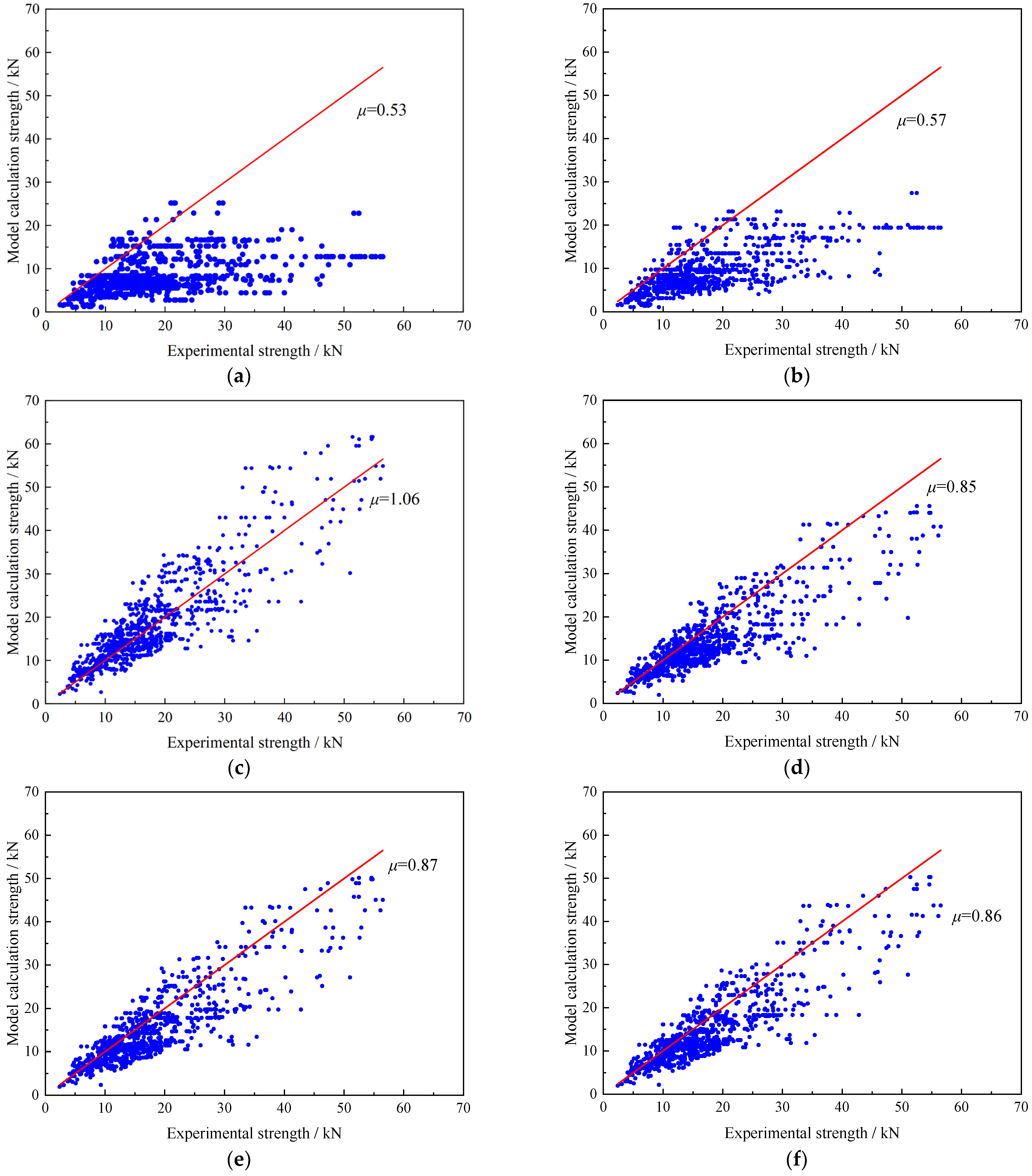
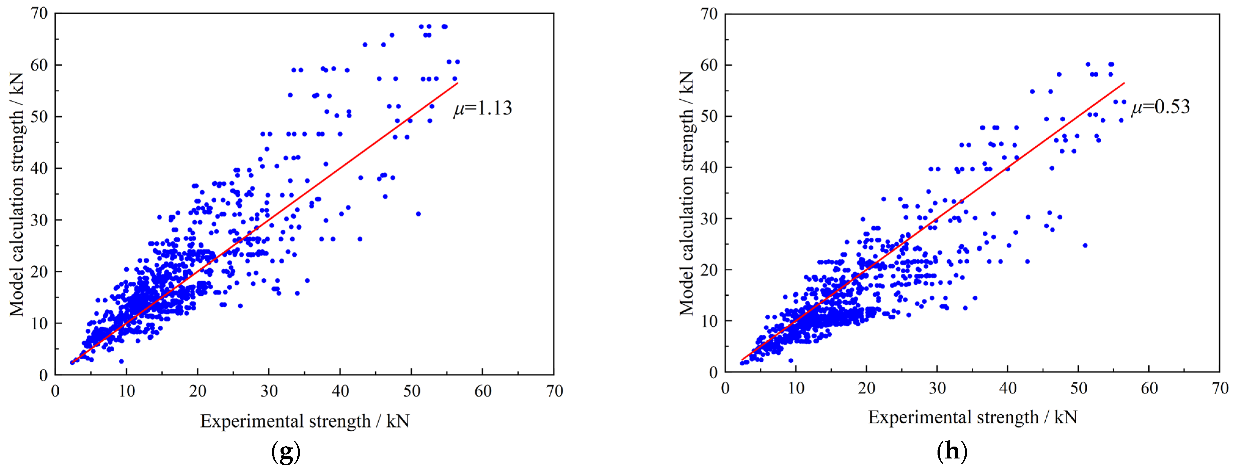
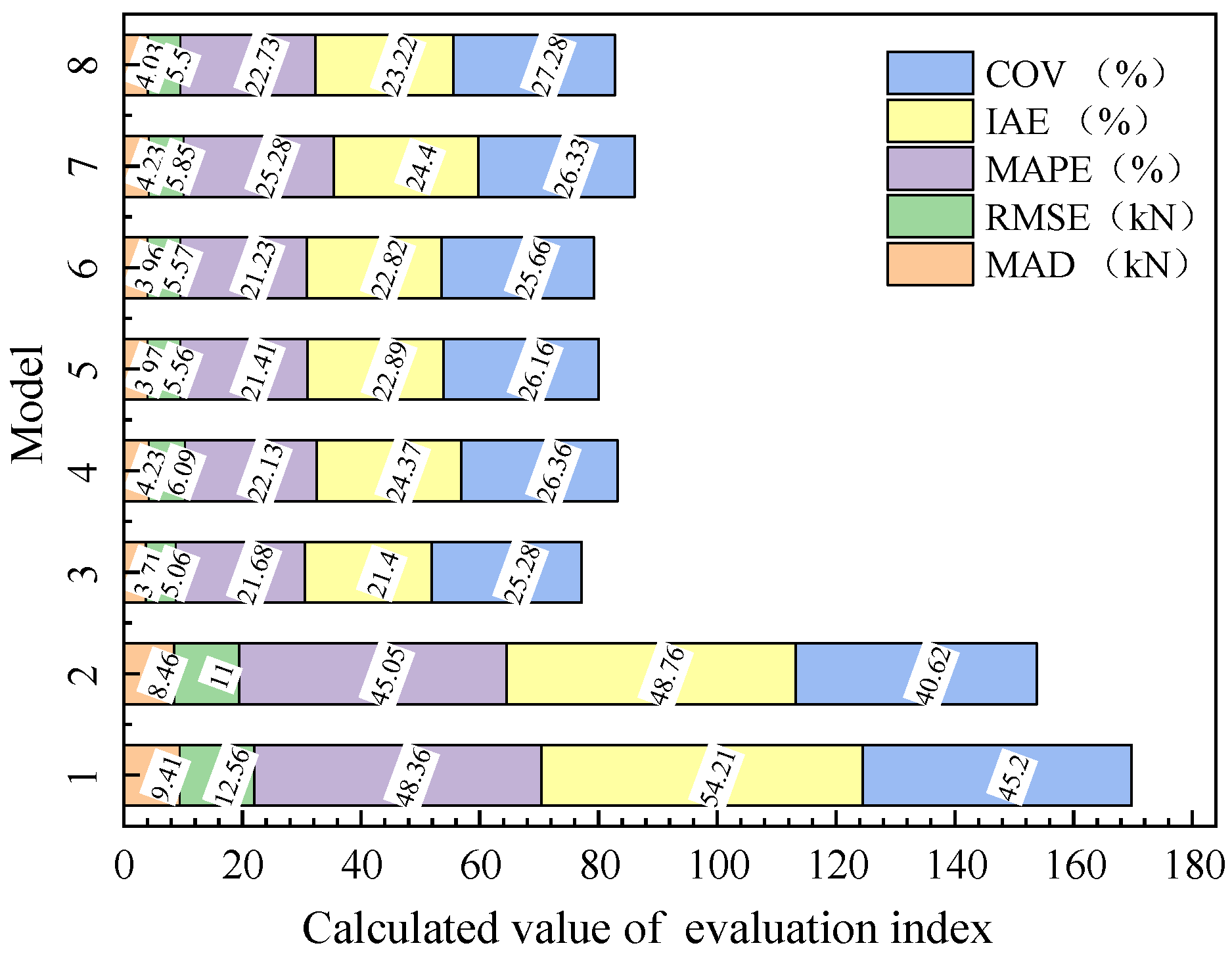
In this study, a total of 1032 FRP–concrete bond strength test data points were collected to establish a single-shear database. Eight existing bond strength models were also reviewed, and their corresponding bond strength values were computed. Given the limitations of conventional neural networks, such as slow convergence and insufficient prediction accuracy—both heavily influenced by the choice of initial weights and thresholds—a genetic algorithm (GA) was adopted to optimize the BP neural network. A GA-based BP neural network model was then developed to predict the bond strength of the collected test data. The predictions obtained from the genetic neural network model were evaluated against the computed results from the eight existing models. Both prediction accuracy and sensitivity analysis were conducted.

2. Collection of Experimental Data and Existing Analytical Models

2.1. Collection of Experimental Data

As illustrated in Figure 1, in a typical single-shear test, an FRP plate was bonded to the surface of a concrete specimen using epoxy resin. The concrete was restrained, and a tensile force was applied to the FRP plate until debonding occurred, from which the corresponding bond strength was derived. Due to material heterogeneity and geometric discontinuities, considerable variability was observed in the experimental results, necessitating a large dataset to enhance the reliability of FRP–concrete bond strength models. In this study, a total of 1032 single-shear test datasets were compiled from existing literature sources [2,3,4,5,6,25,26,27,28,29,30,31,32,33,34,35,36,37,38,39,40,41,42,43] to serve as training and testing inputs for the genetic neural network. Based on the collected data, the primary factors influencing FRP–concrete bond strength included the pull out force (P), the width of the concrete member (b_c), the axial compressive strength of the concrete cylinder (f_c^′), and the width (b_f), elastic modulus (E_f), thickness (t_f), and bond length (L_f) of the FRP plate. In these models, once the bond length exceeded a certain threshold, defined as the effective bond length, the bond strength no longer increased with further extension of the bonded area. The tensile strength of the concrete was calculated using the empirical formula specified in the Chinese code GB 50010-2010 [44], expressed as f_t = 0.395(f_c^′)^0.55.

The ranges of all influencing parameters and their corresponding bond strength values are summarized in

Table 1. Ranges of input parameters and corresponding bond strength values.

Input Parameters	Min	Max
bc (mm)	80	500
fc′ (MPa)	8	75.5
bf (mm)	10	150
Ef (GPa)	18	425.1
tf (mm)	0.083	4
Lf (mm)	29	400
P (kN)	2.4	56.5

Notes: Min and Max are the minimum and maximum values of each influencing factor and bond strength in the collected 1032 test data.

.

2.2. Existing Bond Strength Models

Eight representative models for predicting FRP–concrete bond strength are presented in

Table 2. Existing bond strength calculation model.

ID	Model	Effective Bonding Length	Bond Strength
1	Tanaka [11]	/	$P_{\mathrm{u}}={\tau }_{\mathrm{a}}{b}_{\mathrm{f}}L, {\tau }_{\mathrm{a}}=6.13-\ln L$
2	Yoshizawa [12]	/	$P_{\mathrm{u}}={\tau }_{\mathrm{a}}{b}_{\mathrm{f}}L, {\tau }_{\mathrm{a}}=5.88L^{-0.669}$
3	Neubauer and Rostasy [13]	$L_{\mathrm{e}}=\sqrt{{\displaystyle \frac{E_{\mathrm{f}}{t}_{\mathrm{f}}}{2f_{\mathrm{t}}}}}$	$\begin{array}{l}{P}_{\mathrm{u}}=\left\{\begin{array}{ll}0.64{\kappa }_{\mathrm{w}}{b}_{\mathrm{f}}\sqrt{f_{\mathrm{t}}{E}_{\mathrm{f}}{t}_{\mathrm{f}}}& L\ge L_{\mathrm{e}}\\ 0.64{\kappa }_{\mathrm{w}}{b}_{\mathrm{f}}\sqrt{f_{\mathrm{t}}{E}_{\mathrm{f}}{t}_{\mathrm{f}}}{\displaystyle \frac{L}{L_{\mathrm{e}}}}\left(2-{\displaystyle \frac{L}{L_{\mathrm{e}}}}\right)& L<L_{\mathrm{e}}\end{array}\right.\\ k_{\mathrm{w}}=\sqrt{1.125{\displaystyle \frac{2-b_{\mathrm{f}}/b_{\mathrm{c}}}{1+b_{\mathrm{f}}/400}}}\end{array}$
4	Seracino et al. [16]	$L_{\mathrm{e}}={\displaystyle \frac{\pi }{2\sqrt{{\tau }_{\mathrm{f}}{L}_{\mathrm{per}}/({\delta }_{\mathrm{f}}{E}_{\mathrm{f}}{A}_{\mathrm{f}})}}}$	$\begin{array}{l}{P}_{\mathrm{u}}=\left\{\begin{array}{ll}0.85{\left({\displaystyle \frac{1}{b_{\mathrm{f}}}}\right)}^{0.25}{\left(f_{\mathrm{c}}^{\prime }\right)}^{0.33}\sqrt{L_{\mathrm{per}}{E}_{\mathrm{f}}{A}_{\mathrm{f}}}& L_{\mathrm{f}}\ge L_{\mathrm{e}}\\ 0.85{\displaystyle \frac{L_{\mathrm{f}}}{L_{\mathrm{e}}}}{\left({\displaystyle \frac{1}{b_{\mathrm{f}}}}\right)}^{0.25}{\left(f_{\mathrm{c}}^{\prime }\right)}^{0.33}\sqrt{L_{\mathrm{per}}{E}_{\mathrm{f}}{A}_{\mathrm{f}}}& L_{\mathrm{f}}<L_{\mathrm{e}}\end{array}\right.\\ {\tau }_{\mathrm{f}}=\left(0.802+0.078{\displaystyle \frac{1}{b_{\mathrm{f}}}}\right){\left(f_{\mathrm{c}}^{\prime }\right)}^{0.5}\\ L_{\mathrm{per}}=2+b_{\mathrm{f}}, {\delta }_{\mathrm{f}}={\displaystyle \frac{0.976}{{\tau }_{\mathrm{f}}}}{\left({\displaystyle \frac{1}{b_{\mathrm{f}}}}\right)}^{0.526}{\left(f_{\mathrm{c}}\right)}^{0.6}\end{array}$
5	Matthys [15]	$L_{\mathrm{e}}=\sqrt{{\displaystyle \frac{E_{\mathrm{f}}{t}_{\mathrm{t}}}{2f_{\mathrm{t}}}}}$	$\begin{array}{l}{P}_{\mathrm{u}}=\left\{\begin{array}{ll}0.576k_{\mathrm{b}}{b}_{\mathrm{f}}\sqrt{f_{\mathrm{t}}{E}_{\mathrm{f}}{t}_{\mathrm{f}}}& L\ge L_{\mathrm{e}}\\ 0.576{\displaystyle \frac{L}{L_{\mathrm{e}}}}\left(2-{\displaystyle \frac{L}{L_{\mathrm{e}}}}\right)k_{\mathrm{b}}{b}_{\mathrm{f}}\sqrt{f_{\mathrm{t}}{E}_{\mathrm{f}}{t}_{\mathrm{f}}}& L<L_{\mathrm{e}}\end{array}\right.\\ k_{\mathrm{b}}=1.06\sqrt{{\displaystyle \frac{2-\left(b_{\mathrm{f}}/b_{\mathrm{c}}\right)}{1+\left(b_{\mathrm{f}}/b_{\mathrm{c}}\right)}}}\ge 1\end{array}$
6	Chen and Teng [14]	$L_{\mathrm{e}}=\sqrt{{\displaystyle \frac{E_{\mathrm{f}}{t}_{\mathrm{f}}}{\sqrt{f_{\mathrm{c}}^{\prime }}}}}$	$\begin{array}{l}{P}_{\mathrm{u}}=\left\{\begin{array}{ll}0.427b_{\mathrm{f}}{L}_{\mathrm{e}}{\beta }_{\mathrm{w}}\sqrt{f_{\mathrm{c}}}& L\ge L_{\mathrm{e}}\\ 0.427b_{\mathrm{f}}{L}_{\mathrm{e}}{\beta }_{\mathrm{w}}\sqrt{f_{\mathrm{c}}}\sin {\displaystyle \frac{\pi L}{2L_{\mathrm{e}}}}& L<L_{\mathrm{e}}\end{array}\right.\\ {\beta }_{\mathrm{w}}=\sqrt{{\displaystyle \frac{2-b_{\mathrm{f}}/b_{\mathrm{c}}}{1+b_{\mathrm{f}}/b_{\mathrm{c}}}}}\end{array}$
7	Monti et al. [42]	$L_{\mathrm{e}}=\sqrt{{\displaystyle \frac{E_{\mathrm{f}}{t}_{\mathrm{f}}}{\sqrt{4{\tau }_{\max }}}}}$	$\begin{array}{l}{P}_{\mathrm{u}}=\left\{\begin{array}{ll}{b}_{\mathrm{f}}\sqrt{{\displaystyle \frac{E_{\mathrm{f}}{t}_{\mathrm{f}}{\tau }_{\max }}{3}}}& L\ge L_{\mathrm{e}}\\ b_{\mathrm{f}}\sqrt{{\displaystyle \frac{E_{\mathrm{f}}{t}_{\mathrm{f}}{\tau }_{\max }}{3}}}\sin {\displaystyle \frac{\pi L}{2L_{\mathrm{e}}}}& L<L_{\mathrm{e}}\end{array}\right.\\ {\tau }_{\max }=1.8k_{\mathrm{b}}{f}_{\mathrm{t}}, k_{\mathrm{b}}=\sqrt{1.5{\displaystyle \frac{2-b_{\mathrm{f}}/b_{\mathrm{c}}}{1+b_{\mathrm{f}}/100}}}\end{array}$
8	Kanakubo et al. [43]	$L_{\mathrm{e}}=0.7\sqrt{{\displaystyle \frac{E_{\mathrm{f}}{t}_{\mathrm{f}}}{f_{\mathrm{c}}^{\prime 0.2}}}}$	$P_{\mathrm{u}}=\left\{\begin{array}{ll}1.1f_{\mathrm{c}}^{\prime 0.2}{b}_{\mathrm{f}}{L}_{\mathrm{e}}& L>L_{\mathrm{e}}\\ \left[0.7\cos \left({\displaystyle \frac{L}{L_{\mathrm{e}}}}\right)\pi +1.8\right]f_{\mathrm{c}}^{\prime 0.2}{b}_{\mathrm{f}}L& L<L_{\mathrm{e}}\end{array}\right.$

. The parameters considered in these models are largely consistent with those listed in Table 1. However, it is important to note that in these models, once the bond length exceeds a certain threshold—defined as the effective bond length—the bond strength no longer increases with further extension of the bonded area. The models proposed by Tanaka [11] and Yoshizawa [12] do not account for the effect of the effective bond length. In contrast, the remaining models explicitly incorporate the concept of effective bond length into their formulations.

Using the models listed in Table 2, predictions of bond strength were performed based on the collected dataset. The predicted values from each model were then compared to the experimental values, and a scatter plot illustrating the correlation between experimental and predicted bond strengths is presented in Figure 2. The mean ratio of predicted to experimental values (μ) was used to evaluate model performance, with values closer to 1 indicating higher accuracy. The results show that models ignoring the bond length effect generally yielded lower prediction accuracy, whereas the model proposed by Neubauer and Rostasy [13] achieved a mean ratio of 1.06, indicating relatively high predictive precision.

2.3. Error Analysis

The calculated values of various evaluation metrics comparing the collected experimental data with the predicted results from existing models are presented in Figure 3. The accuracy of each model’s prediction was assessed based on several statistical indicators: mean absolute deviation (MAD), root mean square error (RMSE), mean absolute percentage error (MAPE), and integral of absolute error (IAE). In addition, the dispersion of model predictions was evaluated using the coefficient of variation (CoV). Specifically, MAD represented the average of the absolute deviations between individual observations and their arithmetic mean; RMSE was the square root of the average squared difference between the predicted and actual values; MAPE was a percentage-based transformation of MAD, providing an intuitive sense of prediction accuracy; IAE evaluated the prediction by quantifying the cumulative error area; and CoV, defined as the ratio of the standard deviation to the mean of the predicted values, allowed for comparison across models by eliminating the influence of units and scale.

$$MAD={\displaystyle \frac{1}{n}}{\displaystyle \sum _{i=1}^n\left|{\mathrm{Test}}_i\right.}-\left.{\mathrm{Train}}_i\right|$$

(1)

$$RMSE=\sqrt{{\displaystyle \frac{{\displaystyle \sum _{i=1}^n\left|{\mathrm{Test}}_i\right.-{\left.{\mathrm{Train}}_i\right|}^2}}{n}}}$$

(2)

$$MAPE={\displaystyle \frac{1}{n}}{\displaystyle \sum _{i=1}^n\left|\left.\frac{{\mathrm{Test}}_i-{\mathrm{Train}}_i}{{\mathrm{Test}}_i}\right|\right.}\times 100\%$$

(3)

$$IAE={\displaystyle \sum _{i=1}^n\frac{\left|\left.{\mathrm{Train}}_i-{\mathrm{Test}}_i\right|\right.}{{\displaystyle \sum _{i=1}^n\left|\left.{\mathrm{Test}}_i\right|\right.}}}$$

(4)

$$CoV={\displaystyle \frac{\sqrt{\frac{1}{n}{\displaystyle \sum _{i=1}^n{\left(\frac{{\mathrm{Train}}_i}{{\mathrm{Test}}_i}-\mu \right)}^2}}}{\mu }}$$

(5)

where Test_i denotes the i-th experimental bond strength; Train_i denotes the corresponding predicted value; and μ represents the mean ratio of predicted to experimental values.

As shown in Figure 3, the performance metrics of the models proposed by Tanaka [11] and Yoshizawa [12] were generally found to be inferior to those of the other six models. This was primarily attributed to the fact that these two models did not account for the effective bond length, a factor that has been demonstrated to significantly influence FRP– concrete bond strength. Among the remaining models, the predictions generated by the models of Neubauer and Rostasy [13] and Chen and Teng [14] exhibited the highest accuracy. All associated evaluation indicators yielded lower error values compared to the other models, indicating superior predictive reliability and consistency.

3. Genetic Neural Network Algorithm

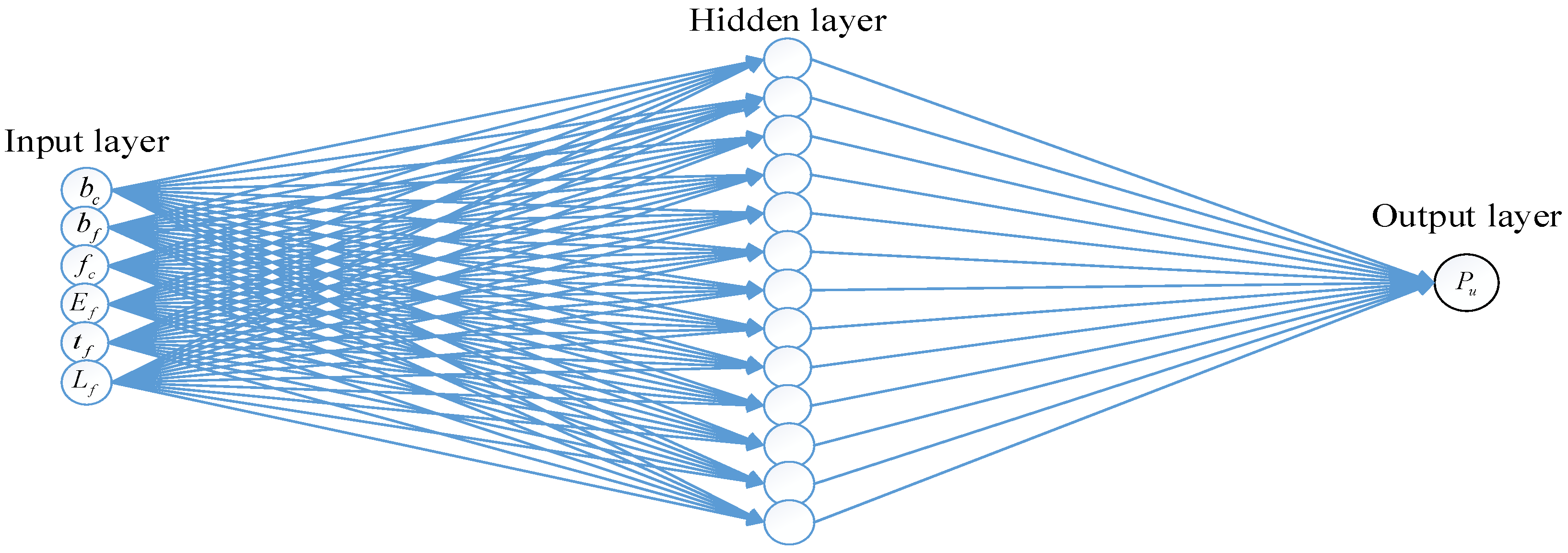
The fundamental principles of the genetic algorithm-optimized backpropagation (GA-BP) neural network are illustrated as Figure 4. The flowchart enclosed within the black box represented the basic framework of the neural network, while the left section outlined the core procedures of the genetic algorithm. The topological structure of the neural network is presented in Figure 5, which consists of three layers: an input layer, a hidden layer, and an output layer. The input layer receives six key parameters that influence the FRP–concrete bond strength. The hidden layer serves as an intermediary to map inputs to outputs, and the output layer generates the predicted bond strength values. The activation function used between the hidden and output layers is a linear (purelin) function, appropriate for regression tasks involving continuous bond strength prediction. The dataset comprising 1032 single-shear test samples was randomly divided into 700 training samples and 332 testing samples (approximately 68% and 32%, respectively). Random sampling was employed due to the continuous nature of the output variable.

The connections between layers were governed by transfer functions, connection weights, and thresholds. The hyperbolic tangent sigmoid function (tansig), as defined in Equation (6), was adopted as the transfer function between the input and hidden layers. The connections between layers were governed by transfer functions, connection weights, and thresholds.

$$\tan \mathrm{sig}\left(n\right)=2/\left[1+\exp \left(-2\ast n\right)\right]-1$$

(6)

The mathematical formulations used to compute the outputs of the hidden and output layers are given in Equations (7) and (8), respectively. S_j denotes the value of the hidden neuron; x_i and y_t represent the actual and predicted outputs, respectively; W_ij and V_ij are the connection weights from the input to the hidden layer and from the hidden to the output layer, respectively; θ_j and γ_t are the biases associated with the hidden and output layers; and f and g represent the activation functions used in each layer. The number of neurons (n₂) in the hidden layer was determined using an empirical formula, i.e., n₂ = 2n₁ + 1, where n₁ denotes the number of output neurons, respectively. The selected configuration is widely adopted in previous studies as a practical approach to balancing model complexity and generalization capability [45,46]. To enhance training efficiency and reduce computational error, the input data were normalized using the mapminmax function.

$$S_{\mathrm{j}}=f\left({\displaystyle \sum _{\mathrm{i}}^n{x}_{\mathrm{i}}{w}_{\mathrm{ij}}-{\theta }_{\mathrm{j}}}\right)$$

(7)

$$y_{\mathrm{t}}=g\left({\displaystyle \sum _{\mathrm{i}}^p{S}_{\mathrm{i}}{v}_{\mathrm{ij}}-{\gamma }_{\mathrm{t}}}\right)$$

(8)

The initial weights and thresholds of the neural network were found to significantly affect training performance. To determine optimal initial parameters, a genetic algorithm was utilized for global optimization. Based on the defined network topology, the number of parameters requiring optimization was calculated. Specifically, the number of weights between the input and hidden layers was n₁ × n₂ = 78, and the number of corresponding biases was n₂ = 13. From the hidden layer to the output layer, the number of weights was n_2*1 = 13, with one additional bias. Therefore, the total number of parameters to be optimized by the genetic algorithm, including all weights and biases, was 105.

The genetic algorithm enhanced both the convergence rate and prediction accuracy of the neural network by optimizing its initial weights and thresholds. Key components of the genetic algorithm included population initialization, fitness evaluation, selection, crossover, and mutation. Each weight or threshold was encoded using a 10-bit binary string, resulting in a chromosome length of 1050 bits. The objective function was defined as the norm of the error between predicted and actual outputs. A rank-based fitness assignment method was adopted, with the fitness calculated as FitnV = ranking(obj), where obj is the objective function value. Selection was carried out using a stochastic tournament method, and crossover was implemented using a single-point approach. The specific parameters used in the genetic algorithm are summarized in

Table 3. Genetic algorithm parameters.

Number of Population	Genetic Algebra	Crossover Probability	Mutation Probability	Generation Gap
100	100	0.7	0.01	0.95

.

4. Data Training and Result Analysis

4.1. Data Training

Based on the modeling approach discussed in Section 2.1, four distinct input variable combinations were selected to assess the prediction performance of the GA-BP neural network. These combinations were used to construct neural networks with different input configurations for comparative analysis. Group 1 employed a six-node input layer with the parameters of b_c, f_c′, b_f, E_f, t_f and L_f. Group 2 used a five-node input layer with the parameters of b_c, f_c′, b_f, (E_f×t_f)^1/2 and L_f. Group 3 also used a five-node input layer with the parameters of b_c, f_c′, E_f, t_f and L_f×b_f. Group 4 adopted a five-node input layer consisting of f_c′, b_f/b_c, E_f, t_f, L_f. All five-node configurations were trained using a hidden layer containing 11 neurons.

Each of the four input configurations underwent a training process using 700 sets of experimental data, where the optimized weights and thresholds obtained from training were subsequently used to predict all 1032 entries in the experimental dataset. The fitness function employed in the genetic algorithm was defined as the Euclidean norm of the prediction error. A rank-based fitness assignment strategy was applied, and the algorithm was terminated either after 100 generations or when the fitness improvement over 10 generations was less than 10⁻⁶. These stopping criteria ensured a balance between convergence stability and computational efficiency. The scatter plots comparing predicted values with experimental results for the four configurations are presented in Figure 6, and the corresponding evaluation metrics are summarized in

Table 4. Evaluation index of each group’s predicted value and test value.

Group	MAD/kN	RMSE/kN	MAPE/%	IAE/%	COV/%
1	2.38	3.25	15.96	13.71	22.22
2	3.05	3.97	20.77	17.61	26.12
3	3.12	4.19	22.94	17.97	35.06
4	4.02	5.49	28.57	23.16	36.84

. To assess potential overfitting, performance metrics were compared between the training and test datasets. The minimal variation observed (e.g., MAD and MAPE in Table 4) indicates strong generalization capability of the model.

4.2. Result Analysis

As shown in Table 4, among all input configurations, the six-node input layer yields the most accurate predictions, with the lowest values across all evaluation metrics. The mean ratio between predicted and experimental bond strengths using the GA-BP neural network is 1.04, indicating the highest predictive precision. Therefore, the GA-BP neural network model with a six-node input layer was selected for final prediction.

The evaluation metrics of the selected GA-BP neural network model with those of the Chen and Teng model and the Neubauer and Rostasy model are shown in Figure 7. “Train” refers to the predictions generated from the first GA-BP neural network model configuration (six-node input), while “C-T” and “N-R” correspond to predictions based on the Chen and Teng and Neubauer and Rostasy models, respectively. The results clearly show that the GA-PA predicted bond strengths exhibit significantly higher accuracy compared to the existing empirical models.

The final optimized weights and thresholds of the GA-BP neural network are listed in

Table 5. Weights and thresholds of genetic neural network.

	IW	LW	b1	b2
Model6-13-1	$\left[\begin{array}{cccccc}0.153& 0.158& 0.345& 0.105& 0.170& -0.489\\ -0.184& -0.484& 0.181& -0.344& 0.298& 0.273\\ 0.191& 0.063& 0.230& 0.196& -0.161& 0.328\\ -0.480& 0.179& 0.238& 0.291& 0.086& -0.163\\ 0.440& 0.314& 0.439& 0.031& 0.196& -0.032\\ -0.330& -0.458& 0.232& 0.329& -0.283& 0.255\\ -0.336& 0.009& -0.328& -0.234& 0.495& 0.161\\ 0.378& 0.485& 0.180& -0.184& -0.341& 0.269\\ 0.071& -0.328& 0.270& -0.251& -0.013& 0.434\\ 0.216& -0.456& 0.378& 0.415& -0.381& 0.363\\ -0.102& 0.106& 0.415& 0.145& -0.077& -0.158\\ 0.212& -0.355& 0.064& -0.320& -0.451& 0.303\\ 0.243& -0.310& 0.372& 0.288& 0.311& -0.239\end{array}\right]$	${\left[\begin{array}{c}0.194 \\ 0.387 \\ 0.088 \\ 0.437 \\ 0.127 \\ 0.263 \\ -0.229 \\ 0.076 \\ -0.424 \\ 0.283 \\ -0.314 \\ -0.270 \\ -0.295 \end{array}\right]}^T$	$\left[\begin{array}{c}-0.387 \\ -0.117 \\ -0.455 \\ -0.075 \\ 0.158 \\ 0.266 \\ 0.332 \\ -0.340 \\ -0.212 \\ 0.263 \\ -0.070 \\ 0.158 \\ -0.365 \end{array}\right]$	$\left[-0.173 \right]$

Notes: IW is the weight from the input layer to the hidden layer; LW is the weight from the hidden layer to the output layer; b₁ is the threshold of the hidden layer neuron; b₂ is the threshold of the output layer neuron.

. The Model_6-13-1 parameters correspond to a neural network with 6 input neurons, 13 hidden neurons, and 1 output neuron. The symbol IW denotes the weight matrix from the input layer to the hidden layer, LW represents the weights from the hidden layer to the output layer, and b₁ and b₂ are the biases for the hidden and output layers, respectively. With these optimized parameters, the network can directly generate predictions without retraining, thus improving computational efficiency.

As shown in Figure 8 and Figure 9, the predicted bond strength values obtained from the GA-BP neural network model versus the experimental values for all 1032 specimens, illustrating the model’s high consistency with experimental data. As shown in Figure 10, it further explores the relationships between the ratio of predicted to experimental values and each of the six input parameters. In these plots, the closer the vertical axis values are to 1, the smaller the prediction deviation and the higher the computational accuracy.

As shown in Figure 10a, the greatest dispersion in predicted values occurred when the width of the concrete member was 100 mm. As the width increased, the dispersion gradually decreased. In Figure 10b, excluding some isolated data points, the highest dispersion was found when the FRP plate width was approximately 45 mm, followed by relatively large dispersion at 100 mm; in contrast, lower dispersion was observed at other widths. According to Figure 10c, the dispersion in predicted values was greatest when the elastic modulus of the FRP plate was 225 GPa, while relatively low dispersion was found under other modulus values. As indicated in Figure 10d, when isolated data points were excluded, the highest dispersion occurred at a concrete compressive strength of 36 MPa. From Figure 10e, it was found that relatively large dispersion appeared when the FRP bond lengths were 100 mm, 150 mm, 200 mm, and 300 mm, while dispersion at other lengths was smaller. As illustrated in Figure 10f, the dispersion in predicted values decreased with increasing FRP plate thickness. The highest dispersion was observed when the thickness ranged from 0.1 mm to 0.2 mm.

Although some prediction errors remained relatively large due to experimental uncertainties, training errors, and inherent limitations of the genetic neural network itself, the proposed model still demonstrated higher accuracy compared to existing bond strength models. This was evidenced by smaller evaluation metric values, indicating that the genetic neural network achieved superior predictive performance for FRP–concrete bond strength.

5. Sensitivity Analysis of Influencing Factors

Sensitivity analysis aims to identify key influential variables among multiple uncertain factors that significantly affect the evaluation metric. In this study, the bond strength was selected as the evaluation indicator, and the six influencing parameters are considered uncertain factors. Sensitivity coefficients are calculated to assess the impact of each factor on the bond strength predicted by different models. The model whose sensitivity response aligns best with experimental data was identified as the optimal one. The sensitivity coefficient S_AF [47,48,49] was calculated as follows:

$$S_{\mathrm{AF}}={\displaystyle \frac{\Delta A/A}{\Delta F/F}}$$

(9)

where A represents the evaluation index; F denotes the uncertain factors; and ΔA and ΔF represent the variations in the evaluation index and the uncertain factor, respectively.

When S_AF < 0, it indicated that the evaluation index was inversely proportional to the uncertain factor. Conversely, when S_AF > 0, a direct proportional relationship was implied. Moreover, a larger absolute value of S_AF suggested a greater sensitivity of the evaluation index to the corresponding uncertain factor. Sensitivity analysis can be categorized into single-factor and multi-factor analyses. In this study, a single-factor sensitivity analysis was adopted. Specifically, six uncertain factors (b_c. f_c′, b_f, E_f, t_f, and L_f) were considered individually to evaluate their influence on the bond strength.

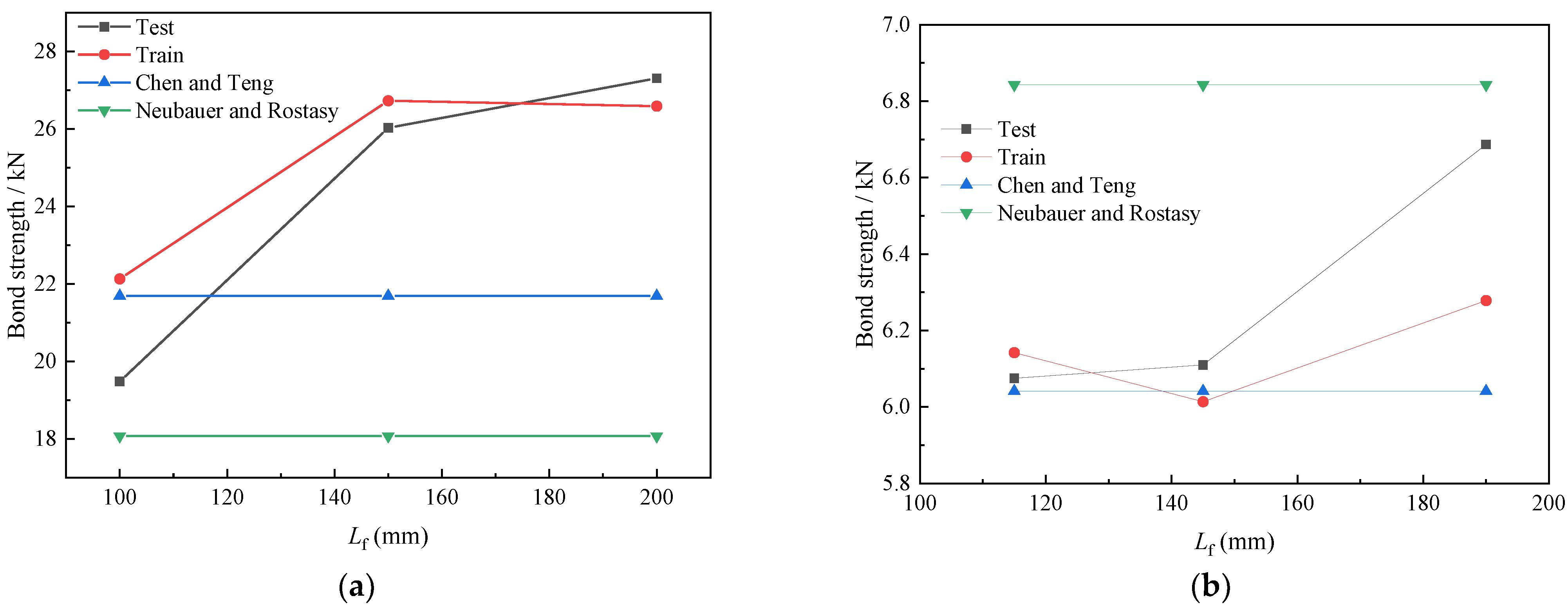
From the 1032 sets of single-shear experimental data, 14 representative samples were selected for analysis. Each influencing parameter’s sensitivity coefficient was computed by averaging the results from two different datasets. As shown in

Table 6. Test data of bond length and bond strength.

Group	bc (mm)	fc′ (MPa)	bf (mm)	Ef (GPa)	tf (mm)	Lf (mm)	Test/kN	Train/kN	C-T/kN	N-R/kN
1	200	40.1	100	240	0.1178	100	19.48	22.13	18.07	21.69
1	200	40.1	100	240	0.1178	150	26.03	26.73	18.07	21.69
1	200	40.1	100	240	0.1178	200	27.31	26.59	18.07	21.69
2	150	23.28	25	256	0.165	115	6.08	6.14	6.04	6.84
2	150	23.28	25	256	0.165	145	6.11	6.01	6.04	6.84
2	150	23.28	25	256	0.165	190	6.69	6.28	6.04	6.84

, the experimental data for cases where the FRP bond length exceeded the effective bond length was predicted by the models. Figure 10b and Figure 11a illustrate the first and second sets of data from Table 6, respectively. Sensitivity analysis was conducted using experimental bond strengths, GA-BP neural network predictions, C-T model values, and (N-R) model values. For samples with multiple experimental values, the average was used for comparison.

When the FRP bond length exceeded the model’s effective length, the averaged sensitivity coefficients obtained from Figure 10b and Figure 11a were 0.278 for experimental values, 0.118 for GA-BP neural network predictions, and 0 for both the C-T and N-R models, indicating insensitivity to bond length in these two traditional models beyond the effective threshold. Similar calculations were conducted for all influencing factors, with the results summarized in

Table 7. Sensitivity coefficient and optimal model.

Group	bc (mm)	fc′ (MPa)	bf (mm)	Ef (GPa)	tf (mm)
bc (mm)	Train	0.105	0.170	0.530	0.310
fc’ (MPa)	C-T	0.125	0.242	0.225	0.248
bf (mm)	N-R	0.795	0.325	0.490	0.590
Ef (GPa)	Train	0.100	0.135	0.440	0.440
tf (mm)	C-T,N-R	0.384	0.222	0.361	0.361
Lf > Le(mm)	Train	0.278	0.118	0.000	0.000
Lf < Le(mm)	Train	0.354	0.313	0.742	0.621

.

The sensitivity coefficients of the genetic neural network predictions for bond strength were found to align more closely with the experimental data compared to other models. The predicted values obtained using the genetic algorithm demonstrated superior performance in the sensitivity analysis.

The relatively low sensitivity coefficient of FRP thickness (t_f) suggests that, within the tested range, variations in thickness have a limited impact on bond strength prediction. This may be attributed to the fact that once the adhesive shear capacity is sufficiently mobilized, further increases in thickness no longer enhance load transfer efficiency. Thus, t_f may be considered a secondary factor, allowing potential simplification in future parametric models. From an experimental design perspective, identifying such low-sensitivity parameters enables researchers to focus resources on more impactful variables, such as f_c′ or b_f, when designing bond tests or strengthening systems. Moreover, the high sensitivity of parameters such as f_c′, b_f, and L_f can be interpreted in terms of physical mechanisms. f_c′ governs the substrate cracking resistance and the initiation of interfacial failure. b_f influences the stress distribution along the interface and may affect the bond shear area. L_f, particularly when below the effective bond length, plays a key role in mobilizing adhesive strength prior to debonding. These connections between data-driven sensitivity analysis and the underlying bond-slip behavior enhance the physical interpretability of the model.

6. Conclusions

(i)

Among the existing models for predicting the bond strength between FRP plates and concrete, those incorporating the concept of effective bond length demonstrated significantly better performance, with prediction errors reduced by up to 35% compared to models that did not include this factor.

(ii)

The optimized neural network architecture, consisting of a 6-node input layer, a 13-node hidden layer, and a 1-node output layer, achieved the highest prediction accuracy. This model yielded a coefficient of determination R² = 0.93, outperforming all benchmark models. The final trained weights and biases can be directly applied to similar prediction tasks, eliminating the need for retraining.

(iii)

A univariate sensitivity analysis using the genetic neural network model revealed that the most influential parameter on bond strength was concrete compressive strength, with a normalized sensitivity coefficient of 0.325. This confirms the model’s ability to capture the influence of key uncertain factors more effectively than traditional approaches.