Article

An Image-Based Concrete-Crack-Width Measurement Method Using Skeleton Pruning and the Edge-OrthoBoundary Algorithm

1
School of Infrastructure Engineering, Dalian University of Technology, Dalian 116024, China
2
China Railway 19th Bureau Group Co., Ltd., Beijing 100176, China
3
China Railway 19th Bureau Group Rail Transit Engineering Co., Ltd., Beijing 101300, China
*
Author to whom correspondence should be addressed.
Buildings 2025, 15(14), 2489; https://doi.org/10.3390/buildings15142489
Submission received: 23 June 2025 / Revised: 9 July 2025 / Accepted: 12 July 2025 / Published: 16 July 2025

Abstract

The accurate measurement of a crack width in concrete infrastructure is essential for structural safety assessment and maintenance. However, existing image-based methods either suffer from overestimation in complex geometries or are computationally inefficient. This paper proposes a novel hybrid approach combining a fast skeleton-pruning algorithm and a crack-width measurement technique called edge-OrthoBoundary (EOB). The skeleton-pruning algorithm prunes the skeleton, viewed as the longest branch in a tree structure, using a depth-first search (DFS) approach. Additionally, an intersection removal algorithm based on dilation replaces the midpoint circle algorithm to segment the crack skeleton into computable parts. The EOB method combines the OrthoBoundary and edge shortest distance (ESD) techniques, effectively correcting the propagation direction of the skeleton points while accounting for their width. The validation of real cracks shows the skeleton-pruning algorithm’s effectiveness, eliminating the need for a specified threshold and reducing time complexity. Experimental results with both actual and synthetic cracks demonstrate that the EOB method achieves the smallest RMS, MAE, and R values, confirming its accuracy and stability compared to the orthogonal projection (OP), OrthoBoundary, and ESD methods.

1. Introduction

Concrete is a widely used material in transportation infrastructure. Due to variations in the load-bearing characteristics of its constituent parts, concrete has a low tensile strength. This makes it susceptible to surface cracks when subjected to mechanical loads, chemical reactions, and environmental factors [1]. These cracks represent the initial stage of concrete distress, leading to spalling, water leakage and steel corrosion. The accurate and rapid detection and measurement of these cracks can lead to surface repairs, pressure grouting, filling, and concrete injection being undertaken, thereby enhancing the safety and durability of concrete structures [2]. Presently, the transportation infrastructure is undergoing a period of maintenance and updating. As existing facilities age and technology advances, the focus has shifted to extending the service life, ensuring functionality, and improving efficiency. This period necessitates a systematic assessment, and the repair, renovation, and reinforcement of existing infrastructure in order to adapt to changing demands and standards. As is demonstrated by the available data, by the year 2020, China had a requirement for the repair of 5.14 million kilometers of roads (representing 90.0% of the total mileage) [3]. A comparable situation could be expected in the United States, where it is estimated that over 618,000 bridges are in need of repair [4]. Conversely, the prevailing approach to concrete crack inspection, characterized by a surge in demand, predominantly relies on manual visual checks. This method is inherently time-consuming and subject to inter-technique variability, impeding the capacity to address the demands arising from the large-scale, expeditious testing of transportation infrastructure. Consequently, there is an imperative demand to develop a rapid and precise method for detecting and measuring cracks.
With the development of image processing technology, many intelligent algorithms have been applied to crack detection. Mohan et al. [5] provided a comprehensive overview of a range of operators and algorithms that are extensively utilized in the field of structural crack detection. These encompass morphological methods such as corrosion and expansion [6], wavelet transforms, Hough transforms [7], Sobel operators, and Canny operators. In environments with insufficient lighting, complex backgrounds, and high noise levels, traditional algorithms are deficient in their precision [8]. Conversely, deep-learning-based algorithms, such as FCN [9], UNET [10], Mask R-CNN [11], DeepLab V3+ [12], CNN [13], DSS-MobileNetV3 [14], and YOLOv8 [15] have demonstrated the capacity to attain high levels of accuracy, which could be classified into four categories: classification, object detection, segmentation, and feature detection [16]. The previously mentioned algorithms have been demonstrated to possess the capability of accurately generating binary images of cracks and backgrounds. However, it should be noted that the intelligent detection algorithms are only capable of localizing the cracks and do not assess their severity [17].
To assess the severity of cracks, further processing of the segmented images is necessary. Among the characteristics of cracks, such as the length, width, and depth, the width is a key indicator that largely determines the severity of a crack [18]. The challenge in crack-width measurement in images lies in the lack of a clear definition. Currently, the mainstream algorithms for calculating crack width can be divided into two methods: one calculates the average scale of the entire crack, while the other computes the width of the crack point by point [18]. The former method calculates the average crack width, which is the area of the crack divided by its length [19]. The primary benefit of this method is its relatively modest computational demand; furthermore, it is capable of producing reliable estimates when the crack boundaries are parallel and the curvature is negligible. In the study of Shan et al. [20], the crack width was assessed using the minimum distance between two sides of crack edge. Yang et al. [9] calculated the mean crack width in road surfaces and building walls under the assumption of no distortion in damage images, utilizing the number of pixels in the crack skeleton as the length of the crack. In a similar vein, Oliveira et al. [19] employed the same calculation method to estimate the width of road surface cracks, resulting in an overestimation of the actual length of the crack skeleton, thereby leading to a smaller crack width. Ji et al. [12] calculated the sum of the Euclidean distances between skeleton points as the length of the crack, obtaining the average width of cracks in asphalt pavements. In the study of Mohammad et al. [21], they hypothesized that a segment of the crack was associated with a strip kernel. They defined the width as the ratio of the intersection area of the crack segment and the strip kernel to the length along the tangent. It is evident that the irregularity of the crack boundaries results in the average width approximating an underestimation of the severity of the cracks.
To enhance the accuracy of crack-width measurement, certain studies have adopted a point-by-point calculation method for crack-width determination [17,18,22]. A mainstream method first extracts the skeleton of the crack and then defines the crack width at a specific point based on the tangential direction or distance of the skeleton points. Liu et al. [23] focused on soil cracks, searching for the minimum Euclidean distance to the nearest boundary points on both sides of the skeleton points as the width at the specific point. Kim et al. [24] and Shan et al. [20] adopted similar algorithms, but the issue with this method is its inability to handle cracks with a high curvature, which can lead to an underestimation of the crack width [17]. Qiu et al. [22] used a principal component analysis (PCA) to calculate the tangential direction of the skeleton points, then projected the vectors formed by the contour points and skeleton points onto an orthogonal basis of the tangential direction to find the two points with the maximum and minimum projection coefficients, using the Euclidean distance between these two points as the crack width. Li et al. [18] proposed an OrthoBoundary algorithm based on the crack boundary and skeleton direction. This algorithm corrected the direction of the skeleton points through the local direction of boundary points. Kim et al. [11] utilized a comparable algorithm; however, it is susceptible to shifts in crack pixels and is influenced by the discrete nature of boundary pixels, which can result in an overestimation of the crack width. Weng et al. [25] developed a novel methodology for measuring crack widths. This approach is predicated on the hypothesis that a small section of a crack exhibits parallel contours. The width of the crack segment is thus defined by the distance shifted on both sides of the enhanced crack edge image from the skeleton of the crack segment. Tang et al. [10] considered the relationship between the slope characteristics at the macro-scale of the crack and the micro-neighborhood features. They proposed a methodology for defining the normals of the skeleton points, with the distance between the normal and the intersection with the boundary defined as the crack width at that point. However, this algorithm is not suitable for crossing cracks. In their seminal paper, Ong et al. [17] proposed a hybrid algorithm that represents a significant improvement on previous methods. This algorithm is based on two fundamental projection techniques: the shortest projection method and the orthogonal projection method. The algorithm takes into account the orthogonal direction of the skeleton points and the constraints of the shortest distance, thereby addressing the issue effectively.
Researchers have also proposed algorithms for calculating a crack width point by point from one boundary of the crack. Zheng et al. [26] calculated the minimum distance from points on one boundary to the other boundary, using the maximum distance among these minimum distances as the maximum width of the crack. Lee et al. [27] estimated the maximum width of cracks in tunnel linings and railway sleepers by calculating the number of pixels that were perpendicular to the crack direction, which provides the shortest distance along the length of the crack. Flah et al. [13] classified cracks in a dichotomous manner, categorizing them into two distinct groups: horizontal and vertical. The maximum boundary distance was calculated based on the height (for vertical cracks) or width (for horizontal cracks) of the images. It is evident that, despite their relative simplicity, these algorithms have the potential to engender substantial deviations, which is a consequence of the simplification of the crack direction at a solitary point. Luo et al. [28] concentrated on the analysis of concrete cracks, employing a finite state machine (FSM) to ascertain the initial and ascending points of the crack, thereby facilitating the determination of its width. However, this algorithm is incapable of handling cracks with non-parallel boundaries in actual scenarios. Wang et al. [29] defined the crack width using Laplace’s equation as a curve similar to the electron trajectory of a capacitor, thereby achieving precise measurements of road surface crack widths. However, it is not suitable for measuring the width of concrete cracks.
It is clear that a point-by-point calculation method for crack-width determination is the mainstream method. However, another problem is that the skeleton extracted by thinning algorithms often contain spurious branches due to the jagged boundaries of cracks, necessitating the use of skeleton-pruning algorithms. Tang et al. [10] employed the eight-neighborhood method for pruning the skeleton, which is only applicable to non-intersecting cracks. Payab et al. [30] defined the points in the upper left and lower right corners of the crack skeleton as endpoints, converting skeleton points into a graph to search for and establish main cracks, pruning portions of non-main cracks based on a length threshold (5% of the length or width); this method is only suitable for non-intersecting cracks. Zhao et al. [31] proposed a method for generating crack-width cloud maps, calculating vector directions of multiple pixels near the bending points in the skeleton points, fitting the generated vectors, and selecting the two vectors with the smallest angles as the main trunk. However, this method tends to retain too much noise for cracks with a large curvature.
To address the above issues, a hybrid method for concrete crack-width measurement in images is proposed. In order to enhance the accuracy of crack-width measurement, this method proposes a fast and effective crack-skeleton-pruning algorithm based on the tree data structure and combines the OrthoBoundary and edge shortest distance (ESD) methods. The remainder of this paper is organized as follows: The “Review of Existing Methods” section introduces the principles of the traditional crack-width measurement methods. The “Methodology” section covers the basic principles of the method, including crack-skeleton extraction, intersection removal, skeleton pruning, and crack-width measurement. The “Experiment validation” section describes the real and synthetic crack measurement experiment for validation, and the “Conclusions” section summarizes the main findings of this research.

2. Review of Existing Methods

2.1. The Orthogonal Projection Method

The orthogonal projection (OP) method proposed by Qiu et al. [22] locates two points closet to the orthogonal vector, as depicted in Figure 1a. First, the crack boundary points are obtained using Canny edge detector. Then, the propagation direction vector of a local region around the skeleton point is determined using the PCA algorithm, with a constant kernel size of five. Once the propagation direction vector has been identified, the orthogonal basis vector can be determined. Next, the projection coefficients of the crack boundary points onto the orthogonal basis vector are calculated and the two corresponding boundary points, which represent the maximum and minimum values, are identified. Finally, the crack width is defined as the Euclidean distance between the two boundary points.

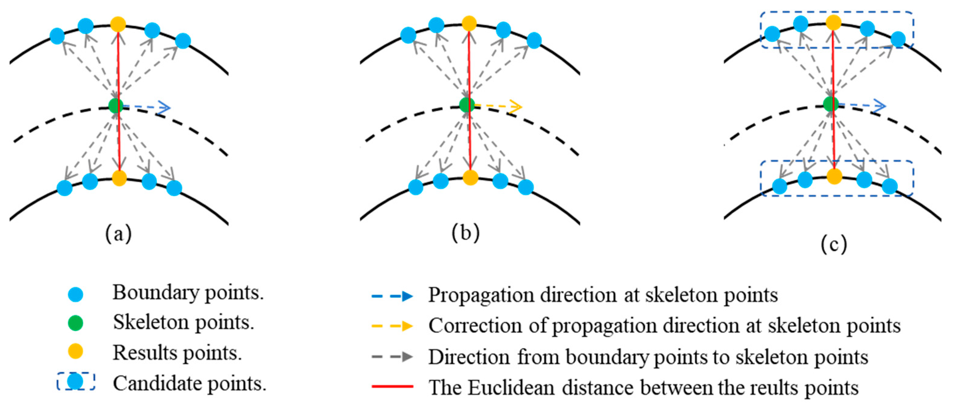
2.2. The OrthoBoundary Method

The OrthoBoundary method proposed by Li et al. [18] is an improvement over the OP method, as shown in Figure 1b. Based on the two boundary points obtained from the OP method, the OrthoBoundary method further optimizes the results. The OrthoBoundary method uses the PCA algorithm to calculate the propagation direction vectors of these two boundary points, converts them into angles in the global coordinate system, and computes the average angle with the propagation direction angle of the skeleton point, which serves as the new propagation direction for the skeleton point. The remaining parts of the OrthoBoundary method are repeated to obtain the two boundary points, and their Euclidean distance is defined as the crack width.

2.3. The Edge Shortest Distance Method

The edge shortest distance (ESD) method proposed by Ong et al. [17] is another improvement over the OP method, as depicted in Figure 1c. Unlike the OP method, the ESD method first obtains the projection coefficients of the unit direction vectors of the crack boundary and skeleton points. It then establishes two thresholds to filter the crack boundary points on both sides. This method defines the shortest Euclidean distance between these points as the crack width. Liu et al. [32] proposed a similar method, which is based on principles similar to those of the ESD method.
In scenarios where multiple cracks exist along the orthogonal direction of the crack-skeleton point, or where the crack exhibits substantial curvature, the OP method tends to produce overestimated results. Although the OrthoBoundary method offers further refinement of the orthogonal direction at the skeleton point, it remains constrained by the OP method’s inherent sensitivity to pixel shift. In contrast, the ESD method does not yield overestimated results due to pixel shifts; rather, its outcomes are contingent upon the propagation direction of the crack-skeleton point. Consequently, the accurate determination and adjustment of this propagation direction are particularly critical for the crack-width measurement.
Figure 1. Principle of existing crack-width measurement methods: (a) OP, (b) OrthoBoundary, and (c) ESD.
Buildings 15 02489 g001

3. Methodology

Figure 2 presents the overall workflow of the proposed method. The process begins with a crack image, from which the crack skeleton is extracted to represent the centerline of the crack using the medial axis transform (MAT). Next, computable crack segments are identified to ensure that only valid and measurable portions of the crack are considered. These segments are then refined through skeleton pruning to eliminate noise and redundant branches. Finally, the crack width is computed based on the pruned skeleton using the edge-OrthoBoundary (EOB) algorithm, enabling the accurate measurement of the crack width from image data.
When collecting crack images, the resolution and shooting distance should meet the requirements for crack detection accuracy while minimizing computation. Based on the thin lens model, the shooting distance u is determined by the following equation [33]:
u = f × 1   + w r w p × p c
where f represents the focal length; w r and w p denote the minimum detectable width in millimeters and in pixels, respectively; and p c is the camera sensor’s resolution in pixels per millimeter.

3.1. Crack-Skeleton Extraction

The crack skeleton is the fundamental structure of crack spots, representing the span of the crack. Two methods for image skeletonization are the medial axis transform (MAT) [34] and the Zhang–Suen algorithm [35], each with distinct characteristics and applicable scenarios. The MAT algorithm is reliant on the geometric properties of the image, thereby providing a more accurate medial axis representation. It is typically employed in conjunction with distance transformations to ascertain distances from skeleton points to the original boundary. Conversely, the Zhang–Suen algorithm exhibits reduced computational complexity, conserves resources, and facilitates the refinement of the crack skeleton. In this regard, we utilize the MAT algorithm for the accurate extraction of the crack skeleton.
As is shown in Figure 3, the MAT algorithm is initiated by the identification of all maximum disks on the segmented image. A maximum disk is defined as a disk that is at a tangent to the boundary at a minimum of two points, with these points not lying within any other disks, as shown in Figure 3b. The centers of these disks are the crack-skeleton points obtained by the MAT algorithm, as is depicted in Figure 3c.

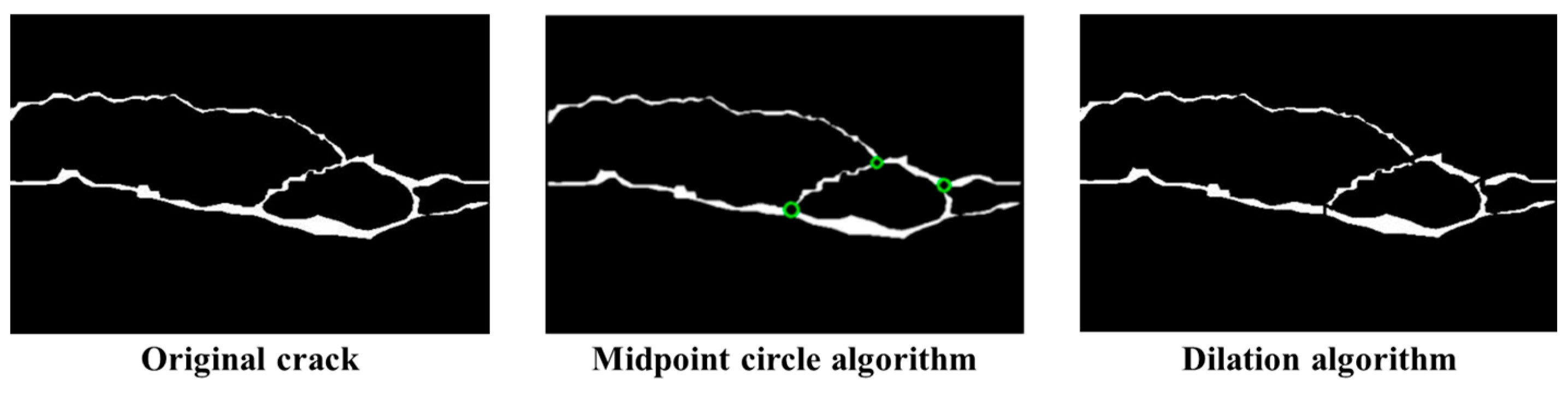
3.2. Intersection Removal

Two issues still need to be addressed after crack-skeleton extraction. Firstly, for a specific skeleton point, the crack width is the gap between the crack surface and the normal material surface, and it should be measured vertically along the span of the crack skeleton. Therefore, there is a lack of measurement definition for the crack width at the intersections of the crack skeleton. It is necessary to remove these intersection points and break them into linear segments. Secondly, due to the jagged boundaries of a crack, the skeleton often contains spurious branches that cannot describe the crack skeleton’s shape but affect the accuracy of the subsequent width measurement.
Previous studies have generally approached these two issues as follows: in the first place, the discrete skeleton evolution (DSE) algorithm developed by Bai et al. [36] is used to trim off the spurious branches; then, the pruned crack skeleton is converted into a graph defined by nodes and edges. The node degrees are then calculated to identify the intersection points (where the node degree is greater than two), after which the midpoint circle algorithm is employed to eliminate the pixels surrounding the intersection points. This process converts a single crack into several computable line segments. However, the DSE algorithm requires the specification of thresholds based on image size and crack width. This can easily lead to under-trimming or over-trimming [17]. It also involves a significant computational load, with the trimming step accounting for the majority of the computational time of the entire width-quantification algorithm [30]. To address these issues, in this paper, we propose a fast and effective crack-skeleton-pruning algorithm based on the graph that contains two parts: intersection removal and skeleton pruning.
As for the segmented binary image, the skeleton S 1 is extracted using the Zhang–Suen algorithm to accelerate the computing speed and reduce spurious branches. After that, the crack boundary B1 is obtained by the Canny edge detector. Then, the jagged boundaries of cracks are eliminated using the cross-shaped dilation function, and the number of iterations for the dilation function is determined through function K, which can be written as follows:
K ( S n ) = | S 1 S n | | S 1 |
where S n denotes the skeleton of the dilated crack. This paper set the condition for K ( S n ) as greater than 0.95 to balance between removing the jagged boundaries and preserving the original skeleton, and the result of this is S * :
S * = S n   |   K ( S n )   >   0 . 95
The skeleton S * is viewed as a graph defined by its nodes and edges. The degree D p i of the skeleton point p i is calculated using the eight-neighborhood method, thus facilitating the end nodes N e ,   intermediate   nodes   N m , and edge points E c :
p i     N e ,   if   D ( p i ) = 1 p i     E c ,   if   D ( p i ) = 2 p i     N cm ,   if   D ( p i )   >   2
where N e represents the end node (the green blocks in Figure 4), E c represents the candidate edge points, and N cm represents the candidate intermediate nodes.
After that, the density-based spatial clustering of applications with noise (DBSCAN) algorithm [37] is employed to cluster N cm into a number of nodes subsets N cm i (the blocks surrounded by the red dashed box in Figure 4). The maximum permissible distance between sample points within the neighborhood is specified as 2 , and the minimum number of samples required for a core point is stipulated as one. For each subset of intermediate nodes N cm i , repeat the following steps: find an adjacent point in E c , move it to set E’, then find an adjacent point in E c that is connected to E’, and continue moving points to E’ until there are no adjacent points left in E c . Next, search for adjacent points in   N e and N cm   to move them to E’, which are the cutting points (the yellow blocks in Figure 4), and move them into E’ until there are no adjacent points left. The result will be the edges E i j (the blue blocks in Figure 4). After repeating the above operations for N cm i , the intermediate nodes N m i will be obtained (the red blocks in Figure 4).
For the cutting points, repeat the following steps: First, as is shown in Figure 5, PCA is used to find the propagation direction θ of a local region at the cutting point, where the kernel size is 5 × 5, and the local region are represented by their local (x, y) coordinates.
θ = tan 1 μ x x μ y y + μ x x μ y y 2 4 μ x y 2 2 μ x y
where μ x x = i N x i x ¯ 2 N + 1 12 , μ y y = i N y i y ¯ 2 N + 1 12 , and μ x y = i N x i y i N .
Next, a one-pixel wide line is drawn at the intersection of the original crack boundary B1 (not the dilated one) with the normal of the cutting point and its opposite direction. After the above steps, the crack skeleton is turned into pieces, which can be viewed as transforming from a graph containing cycles into trees in the view of the data structure.

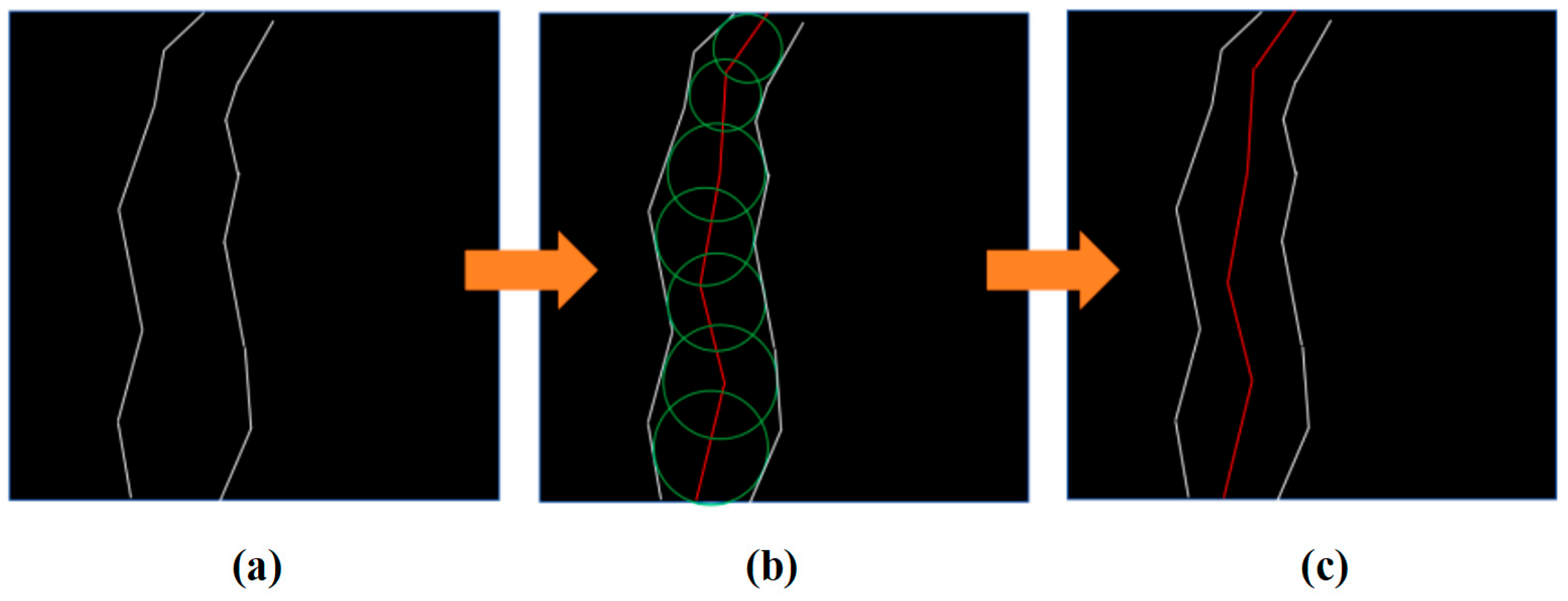
3.3. Skeleton Pruning

Crack-skeleton pruning is carried out to remove unnecessary branches while preserving the supporting structural elements. Thus, this paper defines the crack skeleton as the maximum diameter, or the farthest distance between nodes in the tree structure, which turns the skeleton pruning into the tree’s maximum diameter calculation.
The crack skeleton is extracted using the MAT algorithm and converted into a tree structure. The length l of the edge E i j is determined by the sum of the distance d n   between each pair of points:
d n = x n 1 x n + 2 1 y n 1 y n ,   i f x n 1 x n > y n 1 y n y n 1 y n + 2 1 x n 1 x n ,   i f x n 1 x n y n 1 y n
l = d n
The tree’s maximum diameter is calculated using the depth-first search (DFS) algorithm twice. The DFS algorithm starts from a source node and explores adjacent nodes as deeply as possible until it encounters an endpoint or runs out of unvisited nodes; then, it backtracks to the previous node to continue exploring other paths, which does not require a threshold. Here, the path formed by the tree’s nodes and edges represents the pruned crack skeleton and the crack’s length l s u m is equal to the sum of its edges l n .
l s u m = l n
The overall progress is summarized in Figure 6. For a crack instance, the unpruned skeleton consisting of nodes (red points) and edges (black lines) is viewed as a tree structure. The DFS algorithm calculates the maximum diameter of the tree, which is the crack skeleton after the ‘spurious branches’ have been removed. The skeleton pruning supports the entire span of the crack, yielding a favorable outcome.

3.4. Crack-Width Measurement

This paper proposes a hybrid method, namely the edge-OrthoBoundary (EOB) algorithm, which combines the ESD method and the OB method to measure the crack width, as depicted in Figure 7. For a certain skeleton point p i , its propagation directional angle θ is determined by Equation (5), which in turn yields the unit vector O. For points in the boundary point set B0, the candidate unit vector C i is determined by p i , and the projection coefficient of C i onto O is calculated.
P r o i = O C i
Next, two extreme values,   P r m a x and   P r m i n , can be obtained, and the sets of points that satisfy the following conditions are found as D 1 and D 2 :
D 1 = B [ P P r m a x > 0.999 ]
D 2 = B [ P P r m i n > 0.999 ]
The two points that are closest in distance between D 1 and D 2 are found, and their propagation directional angles θ 1 and θ 2 are calculated by the PCA algorithm. The correction of the propagation directional angle θ is obtained.
θ = θ + θ 1 + θ 2 / 3
After that, Equations (9)–(11) with the corrected propagation direction angle θ are repeated, and the distance between the two points with the closet distance is defined as the crack width.

4. Experiment Validation

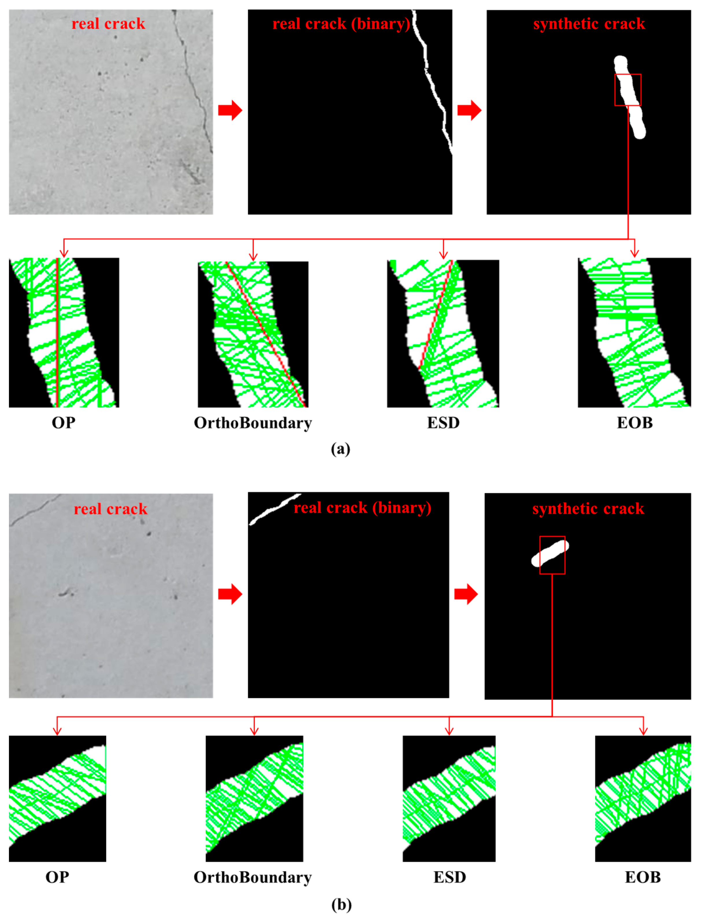
4.1. Real Crack Measurement

In this section, a visual comparison is made between several crack-width measurement methods in real crack-measurement tasks. The CrackForest dataset, comprising 329 crack images with a resolution of 480 × 320 pixels, was employed in this study [38]. The cracks were divided into two categories for discussion: namely cracks with a simple morphology and cracks with multiple intersections.
As for cracks with a simple morphology, there is no need for intersection removal. A comparison of our skeleton-pruning algorithm and the DSE algorithm in two instances (for an oblique crack and horizontal crack) is shown in Figure 8. The threshold for the DSE algorithm is 0.005, which is consistent with the recommendation provided in Li’s study [18]. The DSE algorithm failed the skeleton pruning, as some spurious skeleton branches were retained (see green lines). The pruning results of our algorithm are satisfactory, as the pruned skeleton fitted well with the crack without spurious branches. From the perspective of time complexity, the time complexity of the DSE algorithm is O(n2), while the time complexity of our algorithm is O(n), making it more time-efficient.
As is illustrated in Figure 9, the visual comparison of the width measurement of cracks with a simple morphology is demonstrated using the OP, OrthoBoundary, ESD, and EOB methods, where green lines represent the measured width results. It is evident that the results from the OP and OrthoBoundary methods are overestimated for the crack with a large curvature. However, compared to the results of the OP method, the OB method has fewer unreasonable estimates, demonstrating the effectiveness of its improvements. The width measurements obtained from the ESD and EOB methods are reliable and very close, as both take into account the size and direction of the crack width. As is illustrated in the corners (see red box), the results from the EOB method are more reasonable in terms of direction and size when compared to the ESD method. This is due to the fact that the EOB method corrects the local direction of the crack-skeleton points based on the crack boundary points.
As for the cracks with multiple intersections, a comparison of the midpoint circle algorithm and our intersection removal algorithm is presented in Figure 10. The dilation algorithm successfully eliminates the intersections and breaks them into simple linear segments. This algorithm achieves equivalent results to the midpoint circle algorithm used by Ong et el. [17], but it retains more of the original crack, which is very important in terms of crack quantification and is appropriate for the case where the crack width is only one or two pixels.
Figure 11 depicts the width measurement results of cracks with multiple intersections, where the green lines represent the measured crack width. Both the OP and OrthoBoundary method yield erroneous measurements in the region of a high crack curvature. This is attributable to the method’s sole consideration of direction, resulting in the erroneous identification of boundaries. The error estimation of the OrthoBoundary method is less than that of the OP method, indicating its effectiveness in terms of improvement. Both the ESD method and the EOB method improve its measurement by considering the size factor. In terms of detail, the EOB method has been shown to be superior to the ESD method, as its span is more reasonable, as demonstrated in the red box, due to the boundary-based correction of the crack-width propagation direction.

4.2. Synthetic Crack Measurement

There are ambiguities caused by subjectivity in crack-width measurement manually. Consequently, we generated fitted cracks based on the real crack skeleton to facilitate a comparison of the methods. The real crack skeletons were obtained using the MAT method from 15 pictures of a concrete crack dataset in our previous research [39], where the picture size is 256 × 256 pixels. The cracks in these images were all concrete wall cracks captured under good lighting conditions, including 13 single cracks and 2 intersection cracks, as shown in Figure 12.
The subsequent step involves the delineation of circles with known diameters at the crack-skeleton points. It is imperative to note that the diameter is considered to be the crack width at that particular point p j . The formation of a fitted crack is achieved by centering all circles at the skeleton points, and is placed at the center of a picture sized by 500. All of the pixels of these circles centered at the skeleton points consist of a synthetic crack. The entire process can be seen as the reverse of crack-skeleton extraction.
The OP, OrthoBoundary, ESD, and EOB methods were tested on 15 synthetic cracks with 5941 measured points, with the crack widths ranging from 2 to 30 pixels simulating different widths and filming heights. The results are shown in Table 1. The statistical metrics employed for the quantification of these algorithms included the root mean square error (RMS), mean absolute error (MAE), and Pearson product-moment correlation coefficient (R). The RMS is used to evaluated the accuracy and precision of these algorithms, calculated as shown in Equation (13). The MAE is another metric measuring the accuracy of these methods, calculated as shown in Equation (14), that has low sensitivity to outliers. R can reflect the consistency between the ground truth and the results, which could be calculated by Equation (15).
R M S = 1 n i = 1 n R e i G i 2
M A E = 1 n i = 1 n R e i G i
R = i = 1 n R e i R e ¯ G i G ¯ i = 1 n R e i R e ¯ 2 i = 1 n G i G ¯ 2
where R e i represents the crack-width measurement results of each synthetic crack, R e ¯ represents the mean value of the results, G i represents the crack-width-measurement ground truth of each synthetic crack, G ¯ represents the mean value of the ground truth, and n represents the total number of the synthetic cracks.
The metrics for these methods are summarized in Table 2, and the detailed comparison of these methods is shown in Figure 13. The OP method has the biggest RMS and MAE, and the smallest R. This is caused by its sole consideration of the propagation direction of the skeleton points, with huge overestimation (red line) at the curvatures, as shown in Figure 13a. For the same reason, the OrthoBoundary method also yields overestimates, but it shows some improvements compared to the OP method, presenting more reasonable estimations with smaller RMS and MAE values. The ESD and EOB methods both have acceptable results with a rather small error and high consistency. However, the ESD method still has a small degree of overestimation (red line), as shown in Figure 13a. This is caused by crack’s jagged boundaries. The EOB method outperforms the ESD method by adding the consideration about the boundary points’ prorogation direction, as shown in Figure 13a. When the crack boundary is parallel and has gentle curvatures, all of these methods produce acceptable results, as shown in Figure 13b. In a word, the EOB method performed best with the test images based on the direction and size factors.

5. Conclusions

This paper presents a fast and accurate method for crack-width measurement from images. In addressing the issues of the computation time and the unreasonable removal of branches from the crack skeleton due to the necessity of a specified threshold in the DSE algorithm, this paper proposes a skeleton-pruning algorithm. The skeleton is viewed as the longest branch in the tree data structure and is pruned using the DFS algorithm. In addition, an intersection removal algorithm using the dilation function is proposed in place of the midpoint circle algorithm to break the crack skeleton into computable segments. This paper also presents the EOB method, which combines the OrthoBoundary method and the ESD method. The EOB algorithm simultaneously corrects the propagation direction of the skeleton points and takes into account their width.
The validation of the proposed skeleton-pruning algorithm using real cracks demonstrates its efficacy, obviating the necessity for the specification of a threshold, and exhibiting reduced time complexity. The proposed intersection removal algorithm yields results similar to the midpoint circle algorithm, yet it demonstrates a greater propensity to retain crack pixels. The experimental findings on both actual and synthetic cracks demonstrate that the EOB method exhibits the smallest RMS, MAE, and R when compared to the OP, OB, and ESD methods. This validates the efficacy of the method in terms of accuracy and stability.
The limitation of this method is that the selection of result points during the crack-width measurement relies on a threshold, which affects the accuracy of the results due to the influence of the crack width. In the future, algorithms that do not require a threshold could be developed by judging the relationships between crack boundaries.

Author Contributions

Conceptualization and methodology, C.L. and H.Q.; software, C.L.; validation, Y.T. and H.Q.; formal analysis, H.Z.; investigation, Y.T. and S.P.; resources, J.L. and W.L.; data curation, C.L.; writing—original draft preparation, C.L.; writing—review and editing, H.Q.; supervision, Y.T.; funding acquisition, S.P. All authors have read and agreed to the published version of the manuscript.

Funding

This research was funded by the Central Guidance on Local Science and Technology Development Fund of Liaoning Province (Grant No. 2023JH6/100100054).

Data Availability Statement

The raw data supporting the conclusions of this article will be made available by the authors on request.

Conflicts of Interest

Jinbo Liu and Wenjiang Luo were employed by the company China Railway 19th Bureau Group Rail Transit Engineering Co. The remaining authors declare that the research was conducted in the absence of any commercial or financial relationships that could be construed as a potential conflict of interest.

References

  1. Tao, X.W.; Liu, H.K.; Li, J.; Yu, P.D.; Zhang, J.F. Analysis of Filled Soil-Induced Pier Offset and Cracking in a Highway Bridge and Retrofitting Scheme Development: A Case Study. Buildings 2025, 15, 1929. [Google Scholar] [CrossRef]
  2. Jiang, L.; Han, Q.Q.; Wang, W.J.; Zhang, Y.; Lu, W.; Li, Z. A sugar-coated microbial agent for self-healing cracks in concrete. J. Build. Eng. 2023, 66, 105890. [Google Scholar] [CrossRef]
  3. Ministry of Transport of the People’s Republic of China. Statistical Bulletin on the Development of Transportation Industry 2020. 2020. Available online: https://xxgk.mot.gov.cn/2020/jigou/zhghs/202105/t20210517_3593412.html (accessed on 10 June 2025).
  4. ARTBA. Bridge Conditions Report 2021; ARTBA: Washington, DC, USA, 2021. [Google Scholar]
  5. Arun, M.; Sumathi, P. Crack detection using image processing: A critical review and analysis. Alex. Eng. J. 2018, 57, 787–798. [Google Scholar] [CrossRef]
  6. Yamaguchi, T.; Hashimoto, S. Practical image measurement of crack width for real concrete structure. Electron. Commun. Jpn. 2009, 92, 1–12. [Google Scholar] [CrossRef]
  7. Sohn, H.-G.; Lim, Y.-M.; Yun, K.-H.; Kim, G.-H. Monitoring Crack Changes in Concrete Structures. Comput. Aided Civ. Infrastruct. Eng. 2005, 20, 52–61. [Google Scholar] [CrossRef]
  8. Fan, C.; Ding, Y.; Liu, X.; Yang, K. A review of crack research in concrete structures based on data-driven and intelligent algorithms. Structures 2025, 75, 108800. [Google Scholar] [CrossRef]
  9. Yang, X.C.; Li, H.; Yu, Y.T.; Luo, X.C.; Huang, T.; Yang, X. Automatic Pixel-Level Crack Detection and Measurement Using Fully Convolutional Network. Comput. Aided Civ. Infrastruct. Eng. 2018, 33, 1090–1109. [Google Scholar] [CrossRef]
  10. Tang, Y.C.; Huang, Z.F.; Chen, Z.; Chen, M.Y.; Zhou, H.; Zhang, H.X.; Sun, J.B. Novel visual crack width measurement based on backbone double-scale features for improved detection automation. Eng. Struct. 2023, 274, 115158. [Google Scholar] [CrossRef]
  11. Kim, B.; Cho, S. Image-based concrete crack assessment using mask and region-based convolutional neural network. Struct. Control. Health Monit. 2019, 26, e2381. [Google Scholar] [CrossRef]
  12. Ji, A.K.; Xue, X.L.; Wang, Y.N.; Luo, X.W.; Ru, X.W. An integrated approach to automatic pixel-level crack detection and quantification of asphalt pavement. Autom. Constr. 2020, 114, 103176. [Google Scholar] [CrossRef]
  13. Flah, M.; Suleiman, A.R.; Nehdi, M.L. Classification and quantification of cracks in concrete structures using deep learning image-based techniques. Cem. Concr. Compos. 2020, 114, 103781. [Google Scholar] [CrossRef]
  14. Li, H.; Cheng, Y.; Zhang, Q.; Chen, L. DSS-MobileNetV3: An Efficient Dynamic-State-Space- Enhanced Network for Concrete Crack Segmentation. Buildings 2025, 15, 1905. [Google Scholar] [CrossRef]
  15. Zhang, Y.; Liu, J.; Zhao, Y.; Xu, J.; Wu, W. Crack detection on concrete composite slab using you only look once version 8 based lightweight system. J. Build. Eng. 2025, 108, 112974. [Google Scholar] [CrossRef]
  16. Mario, V.; Cardellicchio, A.; Ruggieri, S.; Nettis, A.; Renò, V.; Uva, G. Artificial intelligence in structural health management of existing bridges. Autom. Constr. 2024, 167, 105719. [Google Scholar] [CrossRef]
  17. Ong, J.C.H.; Ismadi, M.-Z.P.; Wang, X. A hybrid method for pavement crack width measurement. Measurement 2022, 197, 111260. [Google Scholar] [CrossRef]
  18. Li, Z.; Miao, Y.; Torbaghan, M.E.; Zhang, H.F.; Zhang, J.P. Semi-automatic crack width measurement using an OrthoBoundary algorithm. Autom. Constr. 2024, 158, 105251. [Google Scholar] [CrossRef]
  19. Oliveira, H.; Correia, P.L. Automatic Road Crack Detection and Characterization. IEEE Trans. Intell. Transp. Syst. 2013, 14, 155–168. [Google Scholar] [CrossRef]
  20. Shan, B.; Zheng, S.; Ou, J. A stereovision-based crack width detection approach for concrete surface assessment. KSCE J. Civ. Eng. 2016, 20, 803–812. [Google Scholar] [CrossRef]
  21. Jahanshahi, M.R.; Masri, S.F. A new methodology for non-contact accurate crack width measurement through photogrammetry for automated structural safety evaluation. Smart Mater. Struct. 2013, 22, 035019. [Google Scholar] [CrossRef]
  22. Qiu, S.; Wang, W.J.; Wang, S.F.; Wang, K.C. Methodology for accurate AASHTO PP67-10–based cracking quantification using 1-mm 3D pavement images. J. Comput. Civ. Eng. 2017, 31, 04016056. [Google Scholar] [CrossRef]
  23. Chun, L.; Tang, C.S.; Shi, B.; Suo, W.B. Automatic quantification of crack patterns by image processing. Comput. Geosci. 2013, 57, 77–80. [Google Scholar] [CrossRef]
  24. Kim, H.; Lee, J.; Ahn, E.; Cho, S.; Shin, M.; Sim, S.-H. Concrete Crack Identification Using a UAV Incorporating Hybrid Image Processing. Sensors 2017, 17, 2052. [Google Scholar] [CrossRef] [PubMed]
  25. Weng, X.X.; Huang, Y.C.; Wang, W.Z. Segment-based pavement crack quantification. Autom. Constr. 2019, 105, 102819. [Google Scholar] [CrossRef]
  26. Zheng, Y.; Gao, Y.Q.; Lu, S.U.; Mosalam, K.M. Multistage semisupervised active learning framework for crack identification, segmentation, and measurement of bridges. Comput. Aided Civ. Infrastruct. Eng. 2022, 37, 1089–1108. [Google Scholar] [CrossRef]
  27. Lee, J.S.; Hwang, S.H.; Choi, I.Y.; Choi, Y. Estimation of crack width based on shape-sensitive kernels and semantic segmentation. Struct. Control. Health Monit. 2020, 27, e2504. [Google Scholar] [CrossRef]
  28. Luo, Q.J.; Zhen, G.B.; Guo, T.Q. A fast adaptive crack detection algorithm based on a double-edge extraction operator of FSM. Constr. Build. Mater. 2019, 204, 244–254. [Google Scholar] [CrossRef]
  29. Wang, W.J.; Zhang, A.; Wang, K.C.P.; Braham, A.F.; Qiu, S. Pavement Crack Width Measurement Based on Laplace’s Equation for Continuity and Unambiguity. Comput. Aided Civ. Infrastruct. Eng. 2018, 33, 110–123. [Google Scholar] [CrossRef]
  30. Payab, M.; Abbasina, R.; Khanzadi, M. A Brief Review and a New Graph-Based Image Analysis for Concrete Crack Quantification. Arch. Comput. Methods Eng. 2019, 26, 347–365. [Google Scholar] [CrossRef]
  31. Zhao, S.Z.; Kang, F.; Li, J.J. Intelligent segmentation method for blurred cracks and 3D mapping of width nephograms in concrete dams using UAV photogrammetry. Autom. Constr. 2024, 157, 105145. [Google Scholar] [CrossRef]
  32. Liu, Y.; Zhou, T.; Hong, Y.; Pu, Q.H.; Wen, X.G. Neighborhood shortest distance method for concrete crack width detection in images. Eng. Struct. 2025, 326, 119519. [Google Scholar] [CrossRef]
  33. Liu, Y.-F.; Nie, X.; Fan, J.-S.; Liu, X.-G. Image-based crack assessment of bridge piers using unmanned aerial vehicles and three-dimensional scene reconstruction. Comput. Aided Civ. Infrastruct. Eng. 2020, 35, 511–529. [Google Scholar] [CrossRef]
  34. Blum, H.; Nagel, R.N. Shape description using weighted symmetric axis features. Pattern Recognit. 1978, 10, 167–180. [Google Scholar] [CrossRef]
  35. Zhang, T.Y.; Suen, C.Y. A fast parallel algorithm for thinning digital patterns. Commun. ACM 1984, 27, 236–239. [Google Scholar] [CrossRef]
  36. Bai, X.; Latecki, L.J. Discrete Skeleton Evolution. In Proceedings of the Energy Minimization Methods in Computer Vision and Pattern Recognition, Ezhou, China, 27–29 August 2007; Springer: Berlin/Heidelberg, Germany, 2007; pp. 362–374. [Google Scholar]
  37. Ester, M.; Kriegel, H.-P.; Sander, J.; Xu, X. A density-based algorithm for discovering clusters in large spatial databases with noise. In Proceedings of the Second International Conference on Knowledge Discovery and Data Mining, Portland, OR, USA, 2–4 August 1996; pp. 226–231. [Google Scholar]
  38. Shi, Y.; Cui, L.; Qi, Z.; Meng, F.; Chen, Z. Automatic road crack detection using random structured forests. IEEE Trans. Intell. Transp. Syst. 2016, 17, 3434–3445. [Google Scholar] [CrossRef]
  39. Qin, H.; Li, C.; Pan, S.; Wang, Q.; Liu, Y. Three-Dimensional Crack Quantification Using Fused LiDAR Data and Optical Images. J. Comput. Civ. Eng. 2025, 39, 04025045. [Google Scholar] [CrossRef]
Figure 2. Flowchart of the proposed method.
Buildings 15 02489 g002
Figure 3. Crack-skeleton extraction using MAT: (a) segmented image, (b) maximum disks, (c) crack skeleton.
Buildings 15 02489 g003
Figure 4. Crack skeleton transformed into a graph.
Buildings 15 02489 g004
Figure 5. Crack propagation direction determination using PCA algorithm.
Buildings 15 02489 g005
Figure 6. Tree-based maximum diameter crack-skeleton-pruning algorithm.
Buildings 15 02489 g006
Figure 7. Principle of crack-width measurement method: EOB.
Buildings 15 02489 g007
Figure 8. Comparison of skeleton-pruning algorithms.
Buildings 15 02489 g008
Figure 9. Visual comparison of width-measurement algorithms of cracks with simple morphology.
Buildings 15 02489 g009
Figure 10. Visual comparison of intersection removal algorithms.
Buildings 15 02489 g010
Figure 11. Visual comparison of width-measurement algorithms for cracks with multiple intersections.
Buildings 15 02489 g011
Figure 12. Crack images used for width measurement with different algorithms.
Buildings 15 02489 g012
Figure 13. Detailed comparison of synthetic-crack-width measurement results: (a) test on crack with jagged boundaries; (b) test on crack with parallel boundaries.
Buildings 15 02489 g013
Table 1. Results of crack-width measurements for the synthetic cracks.
Crack
No.
Actual Width
(Pixel)
OP
(Pixel)
Relative
Error (%)
OrthoBoundary
(Pixel)
Relative
Error (%)
ESD
(Pixel)
Relative
Error (%)
EOB
(Pixel)
Relative
Error (%)
1223.351067.5%12.21510.5%2.178.5%2.115.5%
245.9147.8%9.50137.5%3.92−2.0%4.164.0%
3620.60243.3%18.43207.2%7.7529.2%7.1619.3%
4820.57157.1%17.56119.5%8.425.3%8.8410.5%
51022.41124.1%15.7357.3%13.5835.8%12.7827.8%
61234.95191.3%24.39103.3%15.0225.2%14.5221.0%
71440.49189.2%27.5296.6%18.5132.2%16.7619.7%
81632.25101.6%24.7654.8%17.7911.2%17.529.5%
91834.2390.2%39.11117.3%20.1612.0%20.8515.8%
102028.6243.1%44.84124.2%21.145.7%22.9014.5%
112255.19150.9%36.4865.8%27.5325.1%25.4815.8%
122445.6390.1%43.6882.0%25.205.0%25.536.4%
132630.2116.2%37.5744.5%26.401.5%27.003.8%
142830.328.3%30.8510.2%27.53−1.7%29.134.0%
153044.3047.7%40.4134.7%34.9816.6%31.083.6%
Table 2. Comparison of metrics for synthetic-crack-width measurement.
MethodRMS (Pixel)MAE (Pixel)R
OP17.5315.270.68
OrthoBoundary13.5112.200.87
ESD2.732.080.98
EOB2.001.720.99
Disclaimer/Publisher’s Note: The statements, opinions and data contained in all publications are solely those of the individual author(s) and contributor(s) and not of MDPI and/or the editor(s). MDPI and/or the editor(s) disclaim responsibility for any injury to people or property resulting from any ideas, methods, instructions or products referred to in the content.

