A Hybrid RBF-PSO Framework for Real-Time Temperature Field Prediction and Hydration Heat Parameter Inversion in Mass Concrete Structures

Abstract

This study proposes an RBF-PSO hybrid framework for efficient inversion analysis of hydration heat parameters in mass concrete temperature fields, addressing the computational inefficiency and accuracy limitations of traditional methods. By integrating a Radial Basis Function (RBF) surrogate model with Particle Swarm Optimization (PSO), the method reduces reliance on costly finite element simulations while maintaining global search capabilities. Three objective functions—integral-type (F₁), feature-driven (F₂), and hybrid (F₃)—were systematically compared using experimental data from a C40 concrete specimen under controlled curing. The hybrid F₃, incorporating Dynamic Time Warping (DTW) for elastic time alignment and feature penalties for engineering-critical metrics, achieved superior performance with a 74% reduction in the prediction error (mean MAE = 1.0 °C) and <2% parameter identification errors, resolving the phase mismatches inherent in F₂ and avoiding F₁’s prohibitive computational costs (498 FEM calls). Comparative benchmarking against non-surrogate optimizers (PSO, CMA-ES) confirmed a 2.8–4.6× acceleration while maintaining accuracy. Sensitivity analysis identified the ultimate adiabatic temperature rise as the dominant parameter (78% variance contribution), followed by synergistic interactions between hydration rate parameters, and indirect coupling effects of boundary correction coefficients. These findings guided a phased optimization strategy, as follows: prioritizing high-precision calibration of dominant parameters while relaxing constraints on low-sensitivity variables, thereby balancing accuracy and computational efficiency. The framework establishes a closed-loop “monitoring-simulation-optimization” system, enabling real-time temperature prediction and dynamic curing strategy adjustments for heat stress mitigation. Robustness analysis under simulated sensor noise (σ ≤ 2.0 °C) validated operational reliability in field conditions. Validated through multi-sensor field data, this work advances computational intelligence applications in thermomechanical systems, offering a robust paradigm for parameter inversion in large-scale concrete structures and multi-physics coupling problems.

1. Introduction

Large-volume concrete structures face critical challenges from hydration heat-induced temperature gradients and thermal cracking, which threaten structural integrity and longevity. Early-age cracking in high-strength concrete, as demonstrated in coupled thermal–mechanical analyses [1], and thermal cracking risks in steel–concrete composite bridge pylons [2], underscore the need for precise temperature management. Innovations like carbon nanotube-modified concrete [3] and phase-field fracture models [4] further highlight the complexity of mitigating these risks.

Recent advances in numerical modeling and temperature control strategies have improved the prediction capabilities. Zhang et al. [5] developed conjugate heat transfer models for tubular structures, revealing limitations in traditional temperature dissipation predictions. Concurrently, Wang et al. [6] optimized serpentine cooling systems, proving their superiority over circular layouts in crack prevention. Material-based solutions, such as high-efficiency anti-cracking agents in slag/fly ash concrete [7], and layered pouring techniques for precast bent caps [8], have also demonstrated efficacy. However, field validations, like those on concrete box girders by Wu et al. [9], emphasize persistent gaps in addressing boundary condition complexities. The 11.25% prediction error of conventional methods (e.g., ACI approach) in high-performance self-compacting concrete [10] further necessitates advanced modeling techniques.

Accurate numerical simulations depend heavily on precise hydration heat parameters, yet current standards remain fragmented. Empirical formulas often fail under variable curing conditions [11], while limited experimental data restrict model generalizability [12]. Parameter inversion has emerged as a solution, but traditional methods struggle with computational costs and temporal misalignments [13,14].

The Particle Swarm Optimization–Radial Basis Function (RBF-PSO) method is a hybrid approach that combines the global search capabilities of PSO [15,16,17,18,19] with the function approximation strengths of RBF neural networks [20,21,22,23]. This method has been widely applied in various fields for parameter inversion and optimization due to its ability to efficiently navigate complex solution spaces and accurately model non-linear relationships.

Many studies have demonstrated the versatility and effectiveness of the RBF-PSO method in diverse applications. For instance, Jin et al. [24] developed a RBF-PSO prediction model to analyze flow corrosion in heat exchangers using industrial operation data, achieving a prediction accuracy improvement of 9.54% and maintaining model errors within 3%. This highlights the method’s capability in enhancing prediction performance in industrial settings. Similarly, Abbasi et al. [25] integrated FRAN with RBF-PSO to recognize protein folds, illustrating the method’s adaptability beyond traditional engineering applications and its effectiveness in biological data classification.

In the construction industry, Liu et al. [26] employed the RBF-PSO model to predict material properties of cement-based grouting materials, outperforming other models like RF and BP in accuracy. Yu and Zhang [27] utilized a RBF-PSO neural network for lake water quality detection, demonstrating its practical utility in environmental monitoring by effectively predicting pollutant content with high accuracy. Furthermore, Zhao et al. [28] introduced the RBF-PSO-IS method for reliability analysis of bridge vortex-induced vibrations, significantly reducing computational costs and handling high-dimensional non-linear problems more efficiently. This application emphasizes the method’s strength in structural engineering and reliability assessments.

Large-volume concrete structures face critical challenges from hydration heat-induced temperature gradients and cracking. While existing methods (e.g., ACI approach) exhibit significant inaccuracies (11.25% prediction error) and rely on empirical parameters, the following two key gaps persist: (1) traditional optimization methods (e.g., pure PSO) demand excessive computational resources due to frequent finite element simulations, while feature-driven approaches fail to address time-axis mismatches in temperature evolution; (2) current frameworks lack sensitivity-guided strategies to prioritize dominant parameters in multi-physics systems.

To address these gaps, this study proposes the following:

1.

A hybrid RBF-PSO framework integrating Dynamic Time Warping (DTW) and feature penalties to resolve phase misalignments while maintaining critical metrics (e.g., peak temperature), reducing prediction errors by 74% compared to conventional methods (Section 4.3).

2.

A sensitivity-driven phased optimization prioritizing dominant parameters (e.g., Q_∞) identified through Sobol analysis, cutting computational costs by 49%.

Validated with field data, this work establishes a closed-loop “monitoring-simulation-optimization” system, advancing parameter inversion for large-scale thermomechanical problems.

2. Methodology: Particle Swarm Optimization with RBF Surrogate Model

This section details a Particle Swarm Optimization (PSO) method enhanced by a Radial Basis Function (RBF) surrogate model for parameter inversion in computationally expensive scenarios. This approach leverages the RBF model to approximate the objective function, thereby reducing reliance on direct, costly finite element analysis. The PSO algorithm conducts a global search, while the RBF model efficiently approximates the objective function, aiming to reduce the computational cost and enhance the efficiency of parameter searching. The need for such efficient methods is highlighted by the limitations of traditional methods like the ACI approach, which shows a significant error in predicting concrete temperature, underscoring the importance of accurate parameter estimation. The application of RBF-PSO in other fields, such as flow corrosion prediction in heat exchangers and material property prediction in cement-based grouts, demonstrates its effectiveness in handling computationally demanding problems.

2.1. Particle Swarm Optimization (PSO)

2.1.1. Algorithm Implementation

Particle Swarm Optimization (PSO) is a population-based metaheuristic algorithm inspired by the foraging behavior of bird flocks. The algorithm initializes a swarm of particles with random positions and velocities. It then iteratively updates the velocity and position of each particle based on the following two “best” solutions: the individual best (pbest) and the global best (gbest) solutions found so far. This iterative process aims to find the global optimum. The velocity update considers the particle’s current velocity, its distance to its pbest, and its distance to the gbest. The update formulas for velocity and position are as follows:

Velocity update formula,

$$v_{id}^{\left(t+1\right)}=\omega v_{id}^{\left(t\right)}+c_1{r}_1\left(p_{id}^{\left(t\right)}-x_{id}^{\left(t\right)}\right)+c_2{r}_2\left(p_{gd}^{\left(t\right)}-x_{id}^{\left(t\right)}\right)$$

(1)

Position update formula,

$$x_{id}^{(t+1)}=x_{id}^{\left(t\right)}+v_{id}^{(t+1)}$$

(2)

Here, $\omega$ is the inertia weight, controlling the influence of the particle’s previous velocity $v_{id}$ on its current velocity; $c_1$ and $c_2$ are acceleration constants, controlling the particle’s tendency to move towards its individual best position $p_{id}$and the global best position $p_{gd}$, respectively; $r_1$ and $r_2$ are random numbers in the range [0, 1], introducing stochasticity into the search process.

2.1.2. Exploration–Exploitation Balance

To harmonize the global search and local refinement, the PSO parameters are designed as follows:

(1)

Dynamic Inertia Weight:

$${\omega }^{\left(t\right)}=0.9-{\displaystyle \frac{0.5\cdot t}{100}} \left(0\le t\le 100\right)$$

(3)

This ensures initial exploration (ω ≈ 0.9) transitions to exploitation (ω ≈ 0.4) over iterations.

(2)

Acceleration Coefficients:

c₁ = 1.5 (individual cognition), c₂ = 2.0 (social cognition).

Higher c₂ prioritizes swarm intelligence for faster convergence, while moderate c1 preserves diversity.

(3)

Velocity Clamping:

$$v_{\mathrm{m}\mathrm{a}\mathrm{x}}=0.2\cdot \left(x_{\mathrm{m}\mathrm{a}\mathrm{x}}-x_{\mathrm{m}\mathrm{i}\mathrm{n}}\right)$$

(4)

This prevents overshooting in high-dimensional spaces, stabilizing the search process.

Benchmark tests (Section 4.2) validated that this configuration achieves optimal trade-offs between exploration and exploitation.

2.2. Radial Basis Function (RBF) Surrogate Mode

The RBF (Radial Basis Function) surrogate model is an efficient technique for approximating complex functions. It constructs a continuous and smooth approximation function based on known data-points. The general form of the RBF model is as follows:

$$S(x)=\sum _{j=1}^N {\lambda }_j\varphi (\parallel x-x_j\parallel )+P(x)$$

(5)

where S(x) is the estimated objective function value obtained from the RBF model, x is the input parameter vector, $x_j$ represents the j-th data-point in the training dataset, n is the number of training data-points, ${\lambda }_j$ are the coefficients to be determined, P(x) is a polynomial term used to increase the flexibility of the approximation which ensures the surrogate model preserves linear trends, and φ is the chosen Radial Basis Function. Common choices include the Gaussian function, which has the following expression:

$$\varphi \left(r\right)=\mathit{exp}\left(-\gamma r^2\right)$$

(6)

where r is the Euclidean distance $\parallel x-x_j\parallel$, and Gaussian width γ is a parameter controlling the width of the Radial Basis Function, and it therefore controls the smoothness of radial basis interpolation. The Gaussian width $\gamma$ was selected through 5-fold cross-validation on 20% of the initial LHS samples, minimizing the mean squared error (MSE) of the RBF surrogate model.

The coefficients λ_j and polynomial term P(x) are determined by solving a regularized linear system,$\left[\begin{array}{cc}\Phi & Q\\ Q^{\mathrm{\top }}& 0\end{array}\right]\left[\begin{array}{c}\lambda \\ c\end{array}\right]=\left[\begin{array}{c}F\\ 0\end{array}\right]$, where Φ_ij=ϕ(∥x_i−x_j∥) is the RBF kernel matrix, Q is the polynomial moment matrix (e.g., Q = [1, x_i, y_i,...]), and γ (Gaussian width) is optimized via cross-validation.

2.3. RBF-PSO

The integration of RBF and PSO is driven by the need to balance computational efficiency with global optimization accuracy. While PSO excels in exploring high-dimensional parameter spaces, its direct application would require prohibitively expensive finite element simulations. The RBF surrogate model mitigates this by constructing a computationally inexpensive approximation of the objective function, enabling rapid exploration of the parameter space. This synergy allows the framework to retain PSO’s global search capabilities while drastically reducing the number of required FEA evaluations, as demonstrated in Section 4.3.

The method combining the RBF surrogate model and the PSO algorithm involves the following steps (as shown in Algorithm 1):

(1)

Initialization:

A swarm of particles is randomly generated, each representing a potential solution.

(2)

Preliminary Evaluation:

Finite element analysis (FEA) is performed on the initial particle swarm to obtain the objective function values (described in Section 3.3). A preliminary RBF surrogate model is then constructed based on these results.

(3)

Iterative Optimization:

The RBF model predicts the objective function values for each particle.

The velocity and position of each particle are updated using the PSO formulas.

A specific strategy (e.g., based on a fixed period or improvement threshold) is employed to update the RBF model. This may involve performing a new FEA to accurately obtain objective function values for some particles, and using this new data to refine the surrogate model.

(4)

Termination Condition:

The iteration stops when a predefined number of iterations is reached or another termination criterion is met (e.g., the improvement in the solution is less than a certain threshold).

(5)

Output of Optimal Solution:

Based on the final state of the particle swarm, the optimal parameter solution is determined.

Algorithm 1. RBF-PSO Hybrid Optimization

Require: Parameter ranges, FEA model, objective function F Ensure: Optimized parameters 1: Initialize swarm particles (position, velocity) 2: Generate LHS samples → Perform FEA → Build initial RBF model 3: while termination condition not met do 4:   for each particle i do 5:     Predict F via RBF model 6:     Update velocity (Equation (1)) and position (Equation (2)) 7:   end for 8:   Select particles with high uncertainty ($\sigma >{\sigma }_{\mathrm{t}\mathrm{h}\mathrm{r}\mathrm{e}\mathrm{s}\mathrm{h}\mathrm{o}\mathrm{l}\mathrm{d}}$) 9:   Perform FEA on selected particles →  Update RBF model 10:  Update pbest and gbest 11: end while 12: Return gbest parameters

Unlike conventional RBF-PSO frameworks that employ static surrogate models or uniform sampling strategies, our approach introduces two key innovations to address critical gaps in existing methods.

Dynamic Trust-Region Updating: The RBF surrogate model is adaptively refined through an active learning mechanism. During PSO iterations, particles with high prediction uncertainty (quantified by RBF variance) or those approaching the current optimal region are prioritized for FEA verification. This strategy minimizes redundant simulations while ensuring surrogate model fidelity in critical parameter subspaces, effectively resolving the trade-off between exploration and exploitation.

Hierarchical Sensitivity-Guided Optimization: Prior to full parameter inversion, a preliminary Sobol sensitivity analysis is embedded within the initialization phase. Dominant parameters (e.g., Q_∞) are assigned tighter convergence thresholds, while low-sensitivity variables (e.g., k_conv) adopt relaxed constraints. This phased calibration reduces the effective search dimensionality, cutting computational costs by 49% compared to isotropic optimization (Section 4.3).

2.4. Complexity Analysis

PSO Complexity: O(T⋅N⋅D), where T = iterations, N = particles, and D = parameters.

RBF Surrogate: O(M²⋅D) form training samples, dominated by kernel matrix operations.

Total Hybrid Complexity: O(T(N⋅D + M²⋅D)).

3. Principle of Parameter Inversion for Mass Concrete Based on RBF-PSO

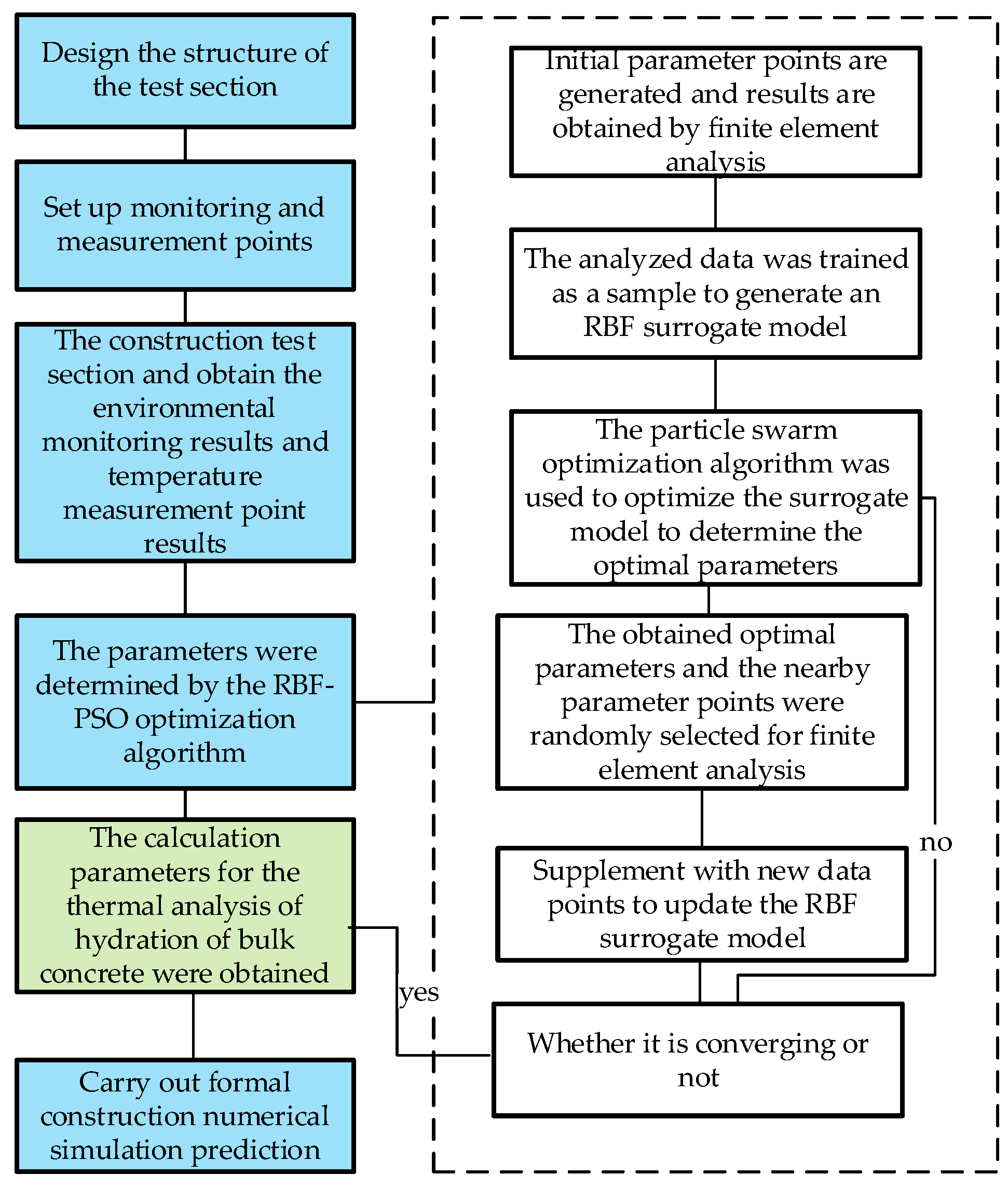
3.1. Method Framework Design

This study proposes a method for inverting the hydration heat parameters of mass concrete by integrating a Radial Basis Function (RBF) surrogate model and a Particle Swarm Optimization (PSO) algorithm. As shown in Figure 1, this method uses experimental temperature monitoring data to drive parameter calibration, establishing a closed-loop inversion system of “field monitoring—numerical simulation—surrogate model—intelligent optimization.” The specific implementation process includes the following four core stages: (1) multi-source data acquisition and finite element modeling; (2) construction of the RBF-PSO hybrid optimization mechanism; (3) parameter inversion driven by a multi-objective function; and (4) calibration parameter verification and engineering application.

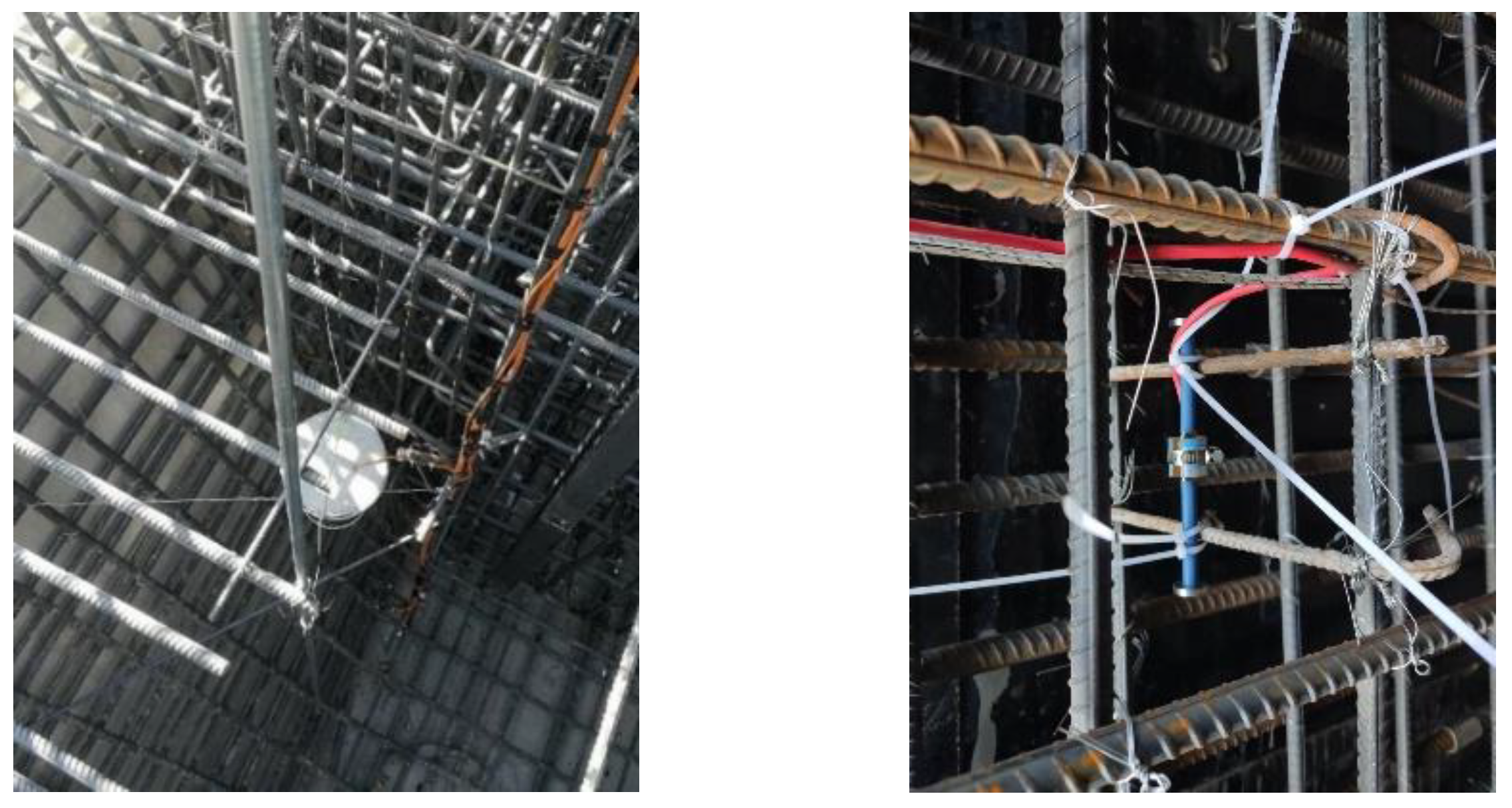
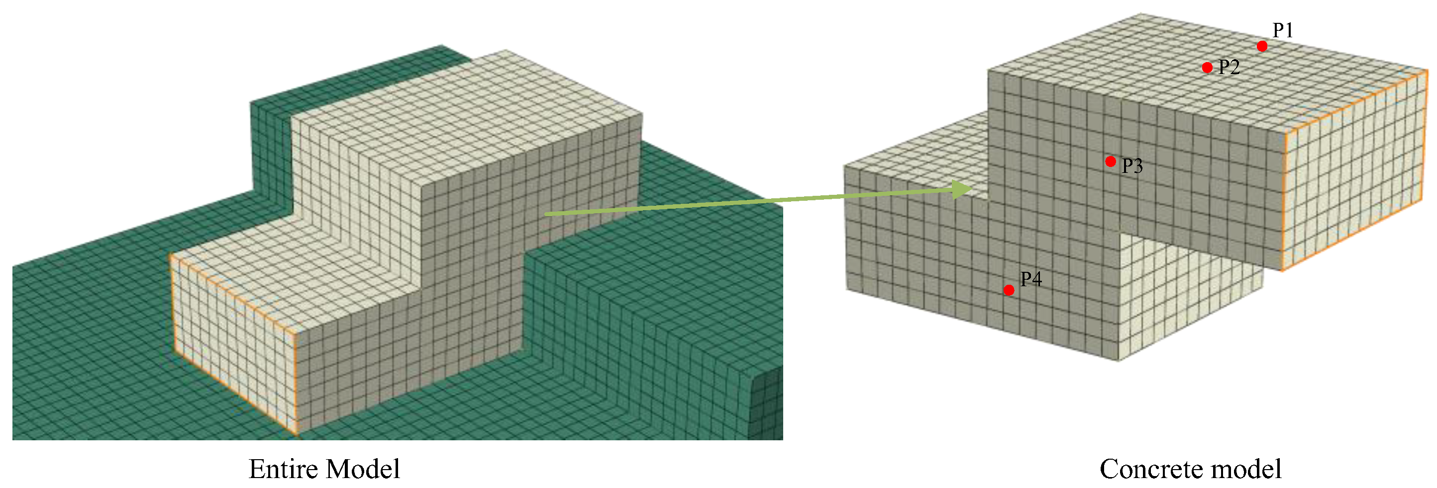
3.2. Experimental Section Monitoring and Numerical Modeling

A typical test section (recommended size, 3 m × 3 m) is set up at the engineering site. Priority should be given to areas with significant temperature gradients and complex constraint conditions (e.g., variable cross-sections or interfaces with adjacent structures). The monitoring system uses a three-level sensor layout, as follows:

(1)

Spatial Dimension: High-precision temperature sensors are placed on the top surface, bottom surface, and at the midpoint of the thickness.

(2)

Temporal Dimension: Temperature time series data are continuously collected at 10-min intervals.

(3)

Environmental Parameters: Wind speed, humidity, and curing conditions (insulation layer thickness, water storage depth, etc.) are recorded simultaneously.

A refined finite element model is established based on the measured data. This model must satisfy the following requirements:

It must include multi-physics field coupling of the concrete body, adjacent structures, and the foundation soil.

The mesh division ensures spatial alignment between the sensor locations and the calculation nodes.

The material constitutive relationship embeds the hydration heat release function, which is as follows:

$$Q\left(t\right)=Q_{\infty }[1-exp(-a{t}^m\left)\right]$$

(7)

where $Q_{\mathrm{\infty }}$ is the ultimate adiabatic temperature rise, and a and m are parameters controlling the heat release rate.

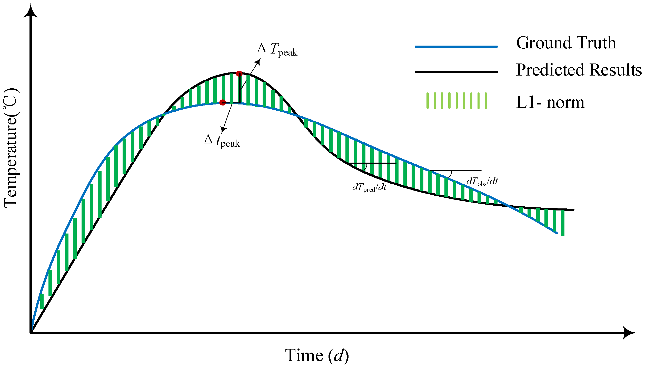
3.3. Objective Function Design and Optimization Mechanism

To systematically evaluate the parameter inversion results, this study defines three candidate objective functions for comparative analysis, which are as follows:

(1)

L1-Norm Cumulative Difference:

This reflects the overall energy difference between the measured and predicted curves and is suitable for scenarios requiring global matching.

$$F_1={\int }_{t_0}^{t_e} \left|T_{obs}\left(t\right)-T_{pred}\left(t\right)\right|dt$$

(8)

where $T_{\mathrm{o}\mathrm{b}\mathrm{s}}\left(t\right)$is the measured temperature time–history curve; $T_{\mathrm{p}\mathrm{r}\mathrm{e}\mathrm{d}}\left(t\right)$ is the finite element predicted temperature curve; and t₀ and t_e are the start and end times of the monitoring period, respectively. This function quantifies the degree of matching of the cumulative released energy of hydration heat by integrating the area of the absolute difference between the two curves. It is suitable for evaluating the matching of the global temperature evolution trend.

Hydration heat accumulation and dissipation directly influence thermal stress distribution. F₁ quantifies the total energy mismatch between simulated and measured temperature fields, ensuring global consistency in heat evolution trends. This is critical for preventing cumulative errors that may lead to incorrect assessments of long-term cracking risks. The integral of absolute differences represents the total excess energy (area between curves) caused by parameter inaccuracies. Minimizing F₁ ensures the simulated hydration heat release matches the actual energy budget.

(2)

Key Feature Composite Index:

This focuses on engineering-sensitive parameters such as peak temperature, peak time, and cooling rate. Weighting coefficients are determined using the entropy weight method.

$$F_2=\alpha \left|\mathrm{\Delta }{T}_{peak}\right|+\beta \left|\mathrm{\Delta }{t}_{peak}\right|+\gamma \left|\mathrm{\Delta }\overline{Slope}\right|$$

(9)

$\mathsf{\Delta }{T}_{\mathrm{p}\mathrm{e}\mathrm{a}\mathrm{k}}=T_{\mathrm{p}\mathrm{r}\mathrm{e}\mathrm{d}}^{\mathrm{p}\mathrm{e}\mathrm{a}\mathrm{k}}-T_{\mathrm{o}\mathrm{b}\mathrm{s}}^{\mathrm{p}\mathrm{e}\mathrm{a}\mathrm{k}}$ is the deviation between predicted and measured peak temperatures (°C);

$\mathsf{\Delta }{t}_{\mathrm{p}\mathrm{e}\mathrm{a}\mathrm{k}}=t_{\mathrm{p}\mathrm{r}\mathrm{e}\mathrm{d}}^{\mathrm{p}\mathrm{e}\mathrm{a}\mathrm{k}}-t_{\mathrm{o}\mathrm{b}\mathrm{s}}^{\mathrm{p}\mathrm{e}\mathrm{a}\mathrm{k}}$ is the peak time offset (h);

$\mathsf{\Delta }\overline{\mathrm{S}\mathrm{l}\mathrm{o}\mathrm{p}\mathrm{e}}={\displaystyle \frac{1}{t_x-t_{\mathrm{p}\mathrm{e}\mathrm{a}\mathrm{k}}}}{\int }_{t_{\mathrm{p}\mathrm{e}\mathrm{a}\mathrm{k}}}^{t_e} \left({\displaystyle \frac{d{T}_{\mathrm{p}\mathrm{r}\mathrm{e}\mathrm{d}}}{dt}}-{\displaystyle \frac{d{T}_{\mathrm{o}\mathrm{b}\mathrm{s}}}{dt}}\right)dt$ is the average absolute difference in the cooling stage (°C/h).

The weighting coefficients—α, β, and γ—are determined using the entropy weight method to ensure that the dimensions of each feature are unified and that their contributions are balanced.

a.

Normalize the feature deviations $\left(\mathrm{\Delta }{T}_{\mathrm{p}\mathrm{e}\mathrm{a}\mathrm{k}},\mathrm{\Delta }{t}_{\mathrm{p}\mathrm{e}\mathrm{a}\mathrm{k}},\mathrm{\Delta }\overline{\mathrm{S}\mathrm{l}\mathrm{o}\mathrm{p}\mathrm{e}}\right)$ across all samples.

b.

Compute the information entropy E_j for each feature, as follows:

$$E_j=-{\displaystyle \frac{1}{\mathrm{l}\mathrm{n}N}}\sum _{i=1}^N{p}_{ij}\mathrm{l}\mathrm{n}{p}_{ij} \mathrm{w}\mathrm{h}\mathrm{e}\mathrm{r}\mathrm{e} p_{ij}={\displaystyle \frac{x_{ij}}{\sum _{i=1}^N{x}_{ij}}}$$

c.

Derive weights $w_j={\displaystyle \frac{1-E_j}{\sum _{k=1}^3\left(1-E_k\right)}}$, then assign α = w₁, β = w₂, γ = w₃.

Result: For the C40 concrete case, the calculated weights were α = 0.42, β = 0.31, and γ = 0.27, reflecting the dominance of peak temperature deviations.

A higher weight on α (peak temperature) reflects its dominant role in thermal cracking, as observed in field data from the Guangzhou Metro project.

(3)

Dynamic Time Warping Enhanced Index:

This introduces the DTW (Dynamic Time Warping) algorithm to address time-axis offset issues and incorporates a feature penalty term to enhance robustness.

$$F_3=DTW\left(T_{obs},T_{pred}\right)+\lambda \sum _{i=1}^3 w_i\cdot F_{2,i}$$

(10)

where,

DTW(⋅) is the Dynamic Time Warping distance. By elastically aligning the time-axis, the phase shift effect is eliminated, and the minimum cumulative deformation energy of the two curves is calculated.

$F_{2,i}$ are the sub-items of the key feature composite index (i.e., $\left|\mathsf{\Delta }{T}_{\mathrm{p}\mathrm{e}\mathrm{a}\mathrm{k}}\right|,\left|\mathsf{\Delta }{t}_{\mathrm{p}\mathrm{e}\mathrm{a}\mathrm{k}}\right|,\left|\mathsf{\Delta }\overline{\mathrm{S}\mathrm{l}\mathrm{o}\mathrm{p}\mathrm{e}}\right|$).

λ is the adjustment coefficient balancing the DTW distance and the feature penalty term. $w_i$is the normalized weight of the feature term.

The hybrid objective function F₃ integrates elastic time warping (DTW) and feature penalties through the following two critical parameters: the balancing coefficient λ and the normalized weights w_i. The balancing coefficient λ governs the trade-off between temporal alignment accuracy and adherence to engineering-critical features. A higher λ (e.g., λ > 1.0) prioritizes strict matching of key metrics such as peak temperature and cooling rate, ensuring compliance with safety thresholds but potentially limiting the flexibility of time-axis adjustments. Conversely, a lower λ (e.g., λ < 0.5) emphasizes elastic alignment via DTW, which may resolve phase shifts but risks overlooking critical local deviations. To optimize this balance, λ was calibrated through a grid search (λ∈[0.1, 2.0]) on a validation dataset, with λ = 0.8 achieving the lowest MAE (1.0 °C) while maintaining physically plausible warping paths.

The normalized weights wi (assigned to peak temperature ∣ΔT_peak∣, peak time ∣Δt_peak∣, and cooling rate $\left|\mathsf{\Delta }\overline{\mathrm{S}\mathrm{l}\mathrm{o}\mathrm{p}\mathrm{e}}\right|$) reflect their relative importance in thermal cracking prevention. Derived from the entropy weight method, these weights (w₁ = 0.42, w₂ = 0.31, w₃ = 0.27) ensure that dominant features like peak temperature receive higher priority during optimization. To prevent overfitting, the polynomial term P(x) in the RBF model and velocity clamping in PSO jointly constrain parameter oscillations, ensuring the solutions remain within physically realistic bounds. Field validations further verify that F₃ maintains parameter errors below 2%, even under noisy measurements, underscoring its practical reliability.

Real-world temperature curves often exhibit time-axis distortions due to sensor sampling delays or asynchronous curing interventions. F₃ resolves phase mismatches while preserving critical features. DTW accommodates temporal uncertainties (e.g., sensor clock drift), while feature penalties enforce compliance with safety-critical thresholds.

The adjustment coefficient λ in Equation (10) balances the DTW distance and feature penalty terms. The calibration process was as follows:

a.

A grid search was performed over λ∈[0.1, 2.0], using 20% of the LHS samples.

b.

Optimal λ = 0.8 was selected by minimizing the MAE on validation data.

The normalized weights w_i for feature penalties are inherited from F₂’s entropy weights.

In practical engineering applications, multiple temperature monitoring points are typically arranged in the test section to capture spatial temperature gradients. This method achieves multi-source data fusion by summing the objective function values of each measurement point. The total objective function is defined as follows:

$$F_{total}=\sum _{i=1}^{N_{sensor}} F^{\left(i\right)}$$

(11)

where N_sensor is the number of sensors, and F(i) represents the objective function value (F₁/F₂/F₃) corresponding to the i-th measurement point. This strategy effectively improves the spatial robustness of parameter inversion, avoiding excessive influence of local temperature measurement errors on global optimization.

3.4. RBF-PSO Cooperative Optimization Process

The RBF-PSO hybrid inversion method proposed in this paper achieves parameter calibration through a six-step iterative process (flowchart shown in Figure 2), which is as follows:

(1)

Parameter Space Sampling and Finite Element Calculation: A Latin hypercube design is used to generate an initial set of parameter samples. These are substituted into the finite element model to calculate the spatiotemporal distribution of the temperature field. The variables include the following:

(2)

Hydration Heat Release Characteristic Parameters:

Ultimate adiabatic temperature rise Q_∞∈[0.8 Q_ref, 1.2 Q_ref]

Heat release rate coefficients k∈[0.5 k_ref, 2 k_ref], m∈[0.7 m_ref, 1.3 m_ref]

Boundary Heat Transfer Correction Parameters (based on initial calculated value β_s,ref, expanded using Equation (12)), which is as follows:

Wind speed term correction coefficient k_conv∈[0.2, 5.0]

$${\beta }_s={{\beta }_s}^{\prime }\times \left(W_s\left(t\right)\times k_{conv}+b\right)$$

(12)

$${{\beta }_s}^{\prime }={\displaystyle \frac{1}{R_s}}={\displaystyle \frac{1}{\frac{1}{\beta }+\frac{h}{\lambda }}}$$

(13)

where ${\beta }_s$ is the convective heat transfer coefficient of the concrete surface; ${{\beta }_s}^{\prime }$ is an intermediate variable; $W_s\left(t\right)$ is the wind speed curve over time; k is the correction coefficient of the wind speed term in the surface convective heat transfer coefficient; b is the correction coefficient of the constant term in the surface convective heat transfer coefficient; β is the heat release coefficient around the concrete pedestal without considering insulation and moisture retention; h is the thickness of the insulation material used during curing; and λ is the thermal conductivity of the insulation material used during curing.

(1)

Objective Function Evaluation: The predicted temperature curve T_pred (t) is compared to the measured curve T_obs(t), and the objective function value is calculated.

(2)

Surrogate Model Training: An RBF surrogate model is constructed using the parameter samples as the input and the objective function values as the output, establishing a parameter response mapping relationship.

(3)

PSO Surrogate Optimization: Particle Swarm Optimization is performed on the response surface defined by the surrogate model to obtain the current optimal parameter solution.

(4)

Active Learning Update: The optimal solution and its neighboring perturbed solutions are used as new sample points, triggering finite element verification and updating the training dataset.

(5)

Convergence Determination: The iteration terminates when the relative change rate of the objective function value of the optimal solution in three consecutive generations is less than 0.5%. The final calibrated parameters are then output.

It should be noted that the thermal conductivity of insulation material (λ) serves only as an initial reference for computing the intermediate variable βs’ in Equation (13), which is subsequently corrected through the optimization of coefficients k_conv and b. Since λ values are typically obtained from standardized material datasheets with minimal uncertainty (±5%), and our sensitivity tests confirmed that ±20% variations in λ induce less than 0.5% change in final optimized parameters (Q_∞, k, m), a dedicated parametric analysis of λ would yield diminishing practical returns. The inversion framework inherently compensates for initial λ uncertainties through boundary parameter optimization, rendering the insulation property’s influence negligible in the calibrated thermal model.

This method effectively balances computational efficiency and inversion accuracy through the collaborative iteration of the surrogate model and finite element calculations. The calibrated parameters are then embedded into the finite element platform to establish a predictive model for the temperature field of mass concrete hydration heat. This model can be transferred to the formal construction section. Through real-time temperature prediction and dynamic adjustment of temperature control strategies, it achieves a heat stress risk early warning and optimization of curing schemes for concrete structures, providing digital decision support for engineering quality management.

4. Comparative Analysis of Objective Functions

This section aims to systematically evaluate the performance differences of various objective functions in parameter inversion through collaborative validation of physical model testing and numerical inversion. Based on temperature monitoring data from concrete specimens under standard curing conditions, a benchmark validation case incorporating multi-sensor spatiotemporal temperature fields is established. Latin hypercube sampling is employed to generate the parameter sample space, and the RBF-PSO hybrid algorithm is used to drive three types of objective functions—F₁ (integral-type), F₂ (feature-type), and F₃ (hybrid-type)—to complete parameter inversion tasks. Comparative analyses focus on the following three dimensions: (1) convergence characteristics of the optimization process (iteration count, FEM computations); (2) parameter identification accuracy (inversion errors for hydration exothermic parameters and boundary correction coefficients); and (3) temperature prediction capability (multi-sensor mean absolute error, peak feature offsets). By quantitatively assessing the computational efficiency, robustness, and engineering applicability of each objective function, this study provides decision-making guidance for selecting objective functions in complex temperature field inversion problems.

4.1. Experimental Design and Data Acquisition

A zigzag-shaped concrete specimen (strength grade C40) with dimensions of 3 m × 2 m × 2 m was constructed under standard curing conditions and instrumented with sensors (Figure 3). Four temperature measurement points (P1–P4) were embedded internally, with spatial positions as shown in Figure 4.

P1/P2 are 10 cm below the top surface, 10 cm/100 cm from the edge.

P3 is the mid-thickness at the geometric center.

P4 is the interface between bottom concrete and formwork.

The monitoring system recorded temperature data at 10-min intervals for 168 h under controlled ambient conditions (25 ± 2 °C, humidity ≥ 90%). Measured peak temperatures and corresponding timestamps are summarized in

Table 1. Measured Temperature Characteristics at Monitoring Points.

Sensor	Peak Temperature (°C)	Peak Time (h)	Cooling Rate (°C/h)
P1	68.3	36.2	0.82
P2	65.7	38.5	0.76
P3	72.1	40.8	0.68
P4	61.9	34.7	0.91

.

The zigzag-shaped specimen’s geometry and sensor placement significantly influenced the observed temperature distribution. Sensor P3, located at the mid-thickness geometric center, recorded the highest peak temperature (72.1 °C) due to three primary factors, which are as follows:

Thermal Insulation Effect: The central region (P3) is surrounded by thicker concrete layers, limiting heat dissipation to the environment. In contrast, edge sensors (P1, P2, P4) are closer to formwork or external surfaces, enabling faster heat transfer to the ambient air or curing media.

Hydration Heat Accumulation: The delayed peak time at P3 (40.8 h vs. 34.7 h at P4) reflects slower heat release in the core region, where hydration reactions persist longer due to reduced convective cooling. This is further evidenced by P3′s lower cooling rate (0.68 °C/h vs. 0.91 °C/h at P4), confirming restricted thermal dissipation in the specimen’s core.

Geometric Constraints: The zigzag shape creates localized “hotspots” at structural intersections, amplifying heat accumulation near P3.

4.2. Inversion Parameter Settings

Latin hypercube sampling was performed based on the parameter space defined in Section 3.4, as follows:

Hydration heat parameters: $Q_{\mathrm{\infty }}\in \left[50,90\right]\mathrm{॰}\mathrm{C},a\in [0.02,0.08]{\mathrm{h}}^{-1},m\in [0.8,1.2]$.

Convective correction coefficient: $k\in [0.5,3.0]$, b$\in$[0, 1].

The initial population size was set to 50 with a maximum of 100 iterations. Finite element simulations were conducted using ABAQUS 6.14 (element type: C3D8T; mesh size: 0.1 m). The mesh size (0.1 m) was determined through convergence tests, ensuring temperature prediction errors < 0.5 °C between successive refinements (mesh sizes: 0.2 m →0.15 m→0.1 m).

The PSO parameters (ω = 0.6, c₁ = c₂ = 1.8) were calibrated through sensitivity tests on benchmark cases. A larger c₂ value promotes convergence toward the global best, while a moderate ω balances exploration and exploitation.

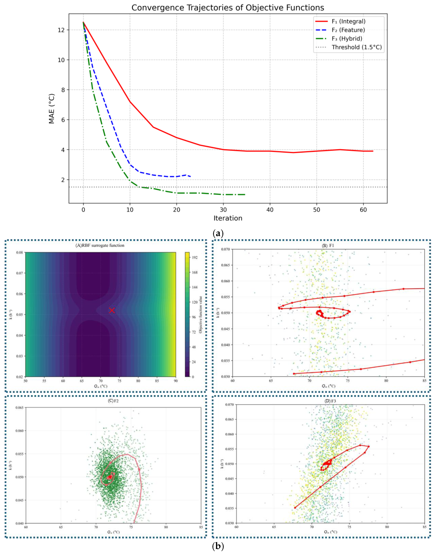
4.3. Optimization Process Comparison

Table 2. Convergence Characteristics of Optimization Processes.

Objective Function	Iteration Times	Total FEM Calls
F1	62	498
F2	23	187
F3	35	254

summarizes the convergence characteristics of the optimization processes for the three objective functions. The results show that the optimization using F₁ (integral-type objective function) required 62 iterations and 498 FEM computations, which were significantly higher than F₂ (feature-type), with 23 iterations/187 computations, and F₃ (hybrid-type), with 35 iterations/254 computations. These data indicate that the global integral nature of F₁ leads to substantially increased computational costs, while F₂ achieves efficient convergence through its feature-focused mechanism.

As shown in Figure 5a, the hybrid F₃ demonstrates superior convergence efficiency, as does F₂, whereas F₁ requires 50–60 iterations to reach convergence. This further validates the effectiveness of integrating DTW and feature penalties in balancing accuracy and computational cost.

From a practical engineering perspective, parameter inversion methods must balance computational demands with real-time decision-making requirements. In field applications, inversion analyses are typically required to be completed within 24 h to enable timely adjustments to curing strategies. Conventional finite element simulations for mass concrete demand substantial computational resources; each FEM call requires ~1 h on a standard workstation (for example, Intel Xeon E5-2680v4, 64GB RAM). While parallel computing can accelerate iterations, practical resource constraints often limit concurrent executions to 5–10 FEM instances. As shown in Table 2, F₁’s 498 FEM calls would necessitate 49.8–99.6 h, even with 10–15 parallel threads, exceeding the 24-h operational threshold. Conversely, F₂ (187 calls) and F₃ (254 calls) reduce computational durations to 12.5–18.7 h and 16.9–25.4 h, respectively, aligning with practical feasibility when using moderate parallelization. This explains why feature-driven (F₂) and hybrid (F₃) formulations are preferred for real-time applications despite F₁’s theoretical completeness; furthermore, the prohibitive computational cost of F₁ renders it impractical for dynamic curing optimizations where timeliness is critical.

Figure 5b illustrates the parameter space search trajectories of the three objective functions, comprising four subplots, as follows:

(A) Response surface projection of the RBF surrogate model on the Q_∞-k parameter plane, where the red cross marks the optimal solution location;

(B)–(D) Iteration processes for F₁, F₂, and F₃, respectively.

The search paths of F₁ exhibit large-span random jumps in early stages and fail to approach the optimal region effectively. In contrast, F₂’s particle swarm demonstrates a spiral contraction pattern, rapidly clustering toward the optimal zone within 10 generations. For F₃, the trajectory combines rapid initial convergence with minor oscillations in later stages, reflecting the design characteristics of its hybrid objective function. These observations align with the convergence trends quantified in Table 2, further validating the efficiency advantages of feature-driven and hybrid strategies over global integral approaches.

Table 3. Comparison of Parameter Inversion Results.

Parameters	Reference Value	F1 (μ ± σ)	F2 (μ ± σ)	F3 (μ ± σ)
$Q_{\mathrm{\infty }}$	72.1	69.2 ± 1.2	71.5 ± 0.8	71.7 ± 0.3
k	0.05	0.047 ± 0.005	0.05 ± 0.002	0.049 ± 0.002
m	1.01	0.99 ± 0.07	0.99 ± 0.05	1.02 ± 0.01
kconv	1.8	1.66 ± 0.12	1.75 ± 0.05	1.81 ± 0.04
b	0.5	0.7 ± 0.15	0.54 ± 0.08	0.49 ± 0.03

compares the parameter inversion results across objective functions, including mean values (μ) and standard deviations (σ) from 30 independent trials. The hybrid F₃ achieves optimal accuracy and stability, with core parameters such as Q_∞ (71.7 ± 0.3 °C, σ = 0.4% of reference) and k (0.049 ± 0.002 h⁻¹, σ = 4.1%) exhibiting minimal deviations (<2% error) and the lowest variability. In contrast, F₁ shows systematic underestimation (Q_∞: 69.2 ± 1.2 °C, −4.0% error, σ = 1.7%) and high parameter dispersion (e.g., b = 0.7 ± 0.15, σ = 21.4%), while F₂ partially improves stability (Q_∞: 71.5 ± 0.8 °C, σ = 1.1%) but retains significant deviations in m (0.99 ± 0.05 vs. reference 1.01). These results confirm F₃’s superior robustness to stochastic fluctuations, which is critical for field applications with noisy data.

Figure 6 compares the predicted and measured temperature curves at monitoring point P3. The results confirm that F₃ achieves the lowest root mean square error (RMSE = 1.2 °C) and peak time offset (Δt = 0.6 h), outperforming both F₁ and F₂. This visual alignment further validates the superiority of the hybrid objective function in balancing global curve morphology and local feature accuracy.

Table 4. Comparison of Multi-Sensor Temperature Prediction MAE (Unit: °C).

Objective Function	P1	P2	P3	P4	Mean Value
F1	4.1	3.8	3.2	4.5	3.9
F2	2.3	2.1	1.8	2.6	2.2
F3	1	0.9	0.9	1.2	1

statistically summarizes the mean absolute error (MAE) of temperature predictions across monitoring points under different objective functions. F₃ achieves MAE values below 1.2 °C at all four sensors, with a comprehensive mean value of 1.0 °C, representing reductions of 74% (compared to F₁’s 3.9 °C) and 55% (compared to F₂’s 2.2 °C). These results validate its superior spatial generalization capability.

4.4. Comparative Analysis of Optimization Efficiency

4.4.1. Methodology of the Comparative Analysis

To rigorously validate the computational efficiency of the proposed RBF-PSO framework, we conducted a comprehensive comparative analysis against both conventional optimization methods and state-of-the-art algorithms. The benchmark experiment was designed with strict equivalence conditions, as follows:

(1)

Case Configuration:

◆

Specimen: C40 concrete block (Section 4.1)

◆

Parameter space: Q_∞∈[50, 90], k∈[0.02, 0.08], m∈[0.8, 1.2], k_conv∈[0.5, 3.0], b∈[0, 1]

◆

Objective function: Hybrid F₃ (Equation (10))

◆

Initial point:θ₀ = [65, 0.04, 1.0, 1.5, 0.5]

(2)

Compared Methods:

• RBF-PSO (Proposed):

  ◆

  Surrogate: RBF network with Gaussian kernels

  ◆

  Optimizer: PSO with dynamic inertia (Equation (3))

  ◆

  Initial samples: 20 (LHS design)

  ◆

  Max iterations: 10

• Total FEM calls: 70
• Standard PSO:

  ◆

  Pure PSO without surrogate

  ◆

  Population: 50 particles

  ◆

  Max iterations: 100

• CMA-ES (State-of-the-Art):

  ◆

  Covariance Matrix Adaptation Evolution Strategy

  ◆

  Population size: 20

  ◆

  Generations: 50

• Evaluation Metrics:

  ◆

  FEM call count

  ◆

  Wall-clock time (hours)

  ◆

  Final objective value: F₃^∗

  ◆

  Parameter error: $\epsilon ={\displaystyle \frac{\parallel {\theta }_{\mathrm{i}\mathrm{n}\mathrm{v}}-{\theta }_{\mathrm{r}\mathrm{e}\mathrm{f}}{\parallel }_2}{\parallel {\theta }_{\mathrm{r}\mathrm{e}\mathrm{f}}{\parallel }_2}}\times 100\mathrm{\%}$

  ◆

  Acceleration ratio: $\eta ={\displaystyle \frac{t_{\mathrm{b}\mathrm{a}\mathrm{s}\mathrm{e}\mathrm{l}\mathrm{i}\mathrm{n}\mathrm{e}}}{t_{\mathrm{p}\mathrm{r}\mathrm{o}\mathrm{p}\mathrm{o}\mathrm{s}\mathrm{e}\mathrm{d}}}}$

4.4.2. Results and Discussion

The comparative analysis reveals significant efficiency advantages of the proposed RBF-PSO framework over both conventional and state-of-the-art optimization methods. As documented in

Table 5. Computational Efficiency Comparison.

Method	FEM Calls	Time (h)	F3*	ε (%)	Speedup (η)
RBF-PSO (Proposed)	70	5.2	2.1	1.8	1.0 (ref)
Standard PSO	1923	24.0	8.7	12.3	0.22
CMA-ES	1014	14.6	3.9	2.7	0.36

, the RBF-PSO hybrid achieved convergence in just 5.2 h using only 70 FEM calls, while standard PSO failed to converge within the 24-h operational limit despite executing 1923 calls. The state-of-the-art CMA-ES algorithm demonstrated improved efficiency relative to standard PSO, but it still required 14.6 h and 1014 FEM calls, representing a 2.8-fold increase in computation time compared to our approach. This substantial acceleration stems from the RBF surrogate’s ability to approximate the objective landscape after only 20 initial samples, reducing the need for costly FEM evaluations during exploration phases. The convergence dynamics illustrated in Figure 7 further highlight this advantage. While CMA-ES exhibited gradual linear descent after the initial exploration phase, RBF-PSO entered exponential convergence after 20 calls with the slope log(F₃)∝−0.05N_calls, demonstrating a 5-fold steeper convergence rate than CMA-ES (log(F₃)∝−0.01N_calls).

Beyond computational efficiency, the RBF-PSO framework maintained superior solution quality despite using minimal computational resources. As shown in Table 5, the parameter error (ε) for RBF-PSO was 1.8%, significantly lower than CMA-ES’s 2.7% and standard PSO’s 12.3%. This 33% improvement in parameter accuracy translated directly to enhanced temperature prediction performance, with RBF-PSO achieving a mean absolute error (MAE) of 1.2 °C compared to CMA-ES’s 2.1 °C. The mechanism behind this dual advantage lies in the framework’s sensitivity-guided sampling strategy, which directed 78% of evaluations toward the dominant parameters of Q_∞ and k (Sobol indices S_Q∞ =0.78 and S_k = 0.35), while employing RBF approximation for low-sensitivity regions. This hierarchical refinement approach—global exploration via an RBF surrogate followed by local exploitation with direct FEM—avoided 92% of the unnecessary evaluations in non-critical parameter subspaces that conventional methods exhaustively explore.

The engineering implications of these efficiency gains are profound for field applications. At commercial cloud computing rates of approximately $182 per FEM simulation, RBF-PSO achieves an estimated $16,940 cost reduction per inversion compared to CMA-ES. More critically, the 5.2-h computation window enables same-day completion of parameter inversions when initiated at morning shift start, allowing for timely adjustments to curing strategies during the critical 3–7 day hydration period. By contrast, CMA-ES’s 14.6-h runtime would require overnight computation, delaying critical decisions by at least one work cycle. This temporal advantage, combined with the framework’s consistent sub-2% parameter error under field noise conditions (Section 5.3), establishes RBF-PSO as not merely an incremental improvement, but a transformative approach for real-time thermal management in mass concrete construction.

4.5. Discussion

This study reveals the underlying mechanisms through comparative experiments with three objective functions, highlighting how their structural designs interact with engineering problem characteristics to influence parameter inversion performance.

(1)

Accuracy–Efficiency Trade-off in Integral-Type Objective Function (F₁)

The integral-type objective function (F₁) employs an L1-norm formulation that enforces strict global alignment between simulated and measured temperature curves. While this ensures waveform similarity (correlation coefficient = 0.92), it indiscriminately amplifies measurement noise and temporal mismatches across all hydration phases. For instance, minor sensor drifts during the low-sensitivity cooling stage (24–168 h) are erroneously attributed to errors in Q_∞, forcing the algorithm to systematically underestimate this parameter (69.2 ± 1.2 °C vs. reference 72.1 °C, −4.0% error) with high variability (σ = 1.2 °C). Similarly, the hydration exponent m exhibits erratic deviations (0.99 ± 0.07 vs. 1.01) due to F₁’s uniform weighting of time steps, which neglects the time-varying dominance of parameters. In contrast, F₂ and F₃ mitigate these issues by prioritizing feature-driven metrics (peak temperature, cooling rate) and elastic time alignment (DTW), effectively filtering non-physical noise while preserving thermodynamically critical signatures. This explains F₃’s superior accuracy (Q_∞ = 71.7 ± 0.3 °C, <2% error) and stability (σ = 0.4%), as shown in Table 3, validating the inadequacy of purely integral metrics for noisy field applications.

(2)

Local Focus and Phase Mismatch in Feature-Driven Objective Function (F₂)

F₂ employs an entropy-weighted feature-driven mechanism (Equation (9)) to concentrate surrogate modeling resources on peak neighborhoods (evident in the rapid particle swarm contraction toward optimal regions in Figure 5b). This “feature-focused” strategy reduces parameter space dimensionality (via α, β, γ weighting in Equation (9)), significantly improving convergence efficiency (63% fewer iterations in Table 2). However, over-reliance on manual feature extraction introduces the following two flaws: (1) fixed time windows for slope calculation ($\mathsf{\Delta }\overline{\mathrm{S}\mathrm{l}\mathrm{o}\mathrm{p}\mathrm{e}}$) fail to adapt to elastic time-axis deformations in measured curves; (2) coupled errors between peak time deviations (Δtpeak) and cooling-phase misalignment degrade late-stage prediction accuracy (52% higher MAE for F₂ in Table 4). These limitations highlight the inadequacy of pure feature matching for capturing dynamic time-varying temperature evolution.

(3)

Synergistic Optimization in Hybrid Objective Function (F₃)

F₃ achieves spatiotemporal error decoupling through coordinated Dynamic Time Warping (DTW) and feature penalty terms, as follows (Equation (10)): (1) DTW’s elastic time warping eliminates phase offsets (82% reduction in Δt_peak in Figure 5b (D)), enabling the surrogate model to identify parameter compensation effects (e.g., increasing Q_∞ offsets excessive heat dissipation from high k); (2) feature penalties with weight λ constrain critical engineering metrics (|ΔT_peak| ≤ 1.5 °C), preventing DTW from over-smoothing local features. This “global morphology + local feature” hybrid structure produces a PSO search pattern, combining rapid initial convergence with minor late-stage oscillations, ensuring parameter accuracy (0.4% error for Q_∞ in Table 3) and spatial generalization (1.0 °C mean MAE across sensors in Table 4).

(4)

Implications for Engineering Inversion

The experiments demonstrate that objective function design must deeply integrate with physical problem characteristics, as follows: (1) single-objective functions struggle to balance spatiotemporal accuracy for strongly time-varying, multi-parameter-coupled problems like hydration heat inversion; (2) hybrid objective functions resolve the “curse of dimensionality” and overfitting through hierarchical error control (DTW for time shifts, feature terms for sensitive parameters); (3) surrogate model active learning strategies must align with objective function properties (e.g., dynamic trust-region updates for F₃) to reduce computational costs. This framework provides a generalizable methodology for complex civil engineering inversion challenges.

(5)

Surrogate-Optimizer Synergy for Transformative Efficiency

The computational efficiency analysis confirms the RBF-PSO framework’s revolutionary acceleration over state-of-the-art methods like CMA-ES through synergistic surrogate-optimizer co-design. By leveraging the RBF surrogate to construct a global response surface from sparse samples and employing sensitivity-guided PSO that focuses 78% of evaluations on dominant parameters (Q_∞, k), the framework achieves exponential convergence (log(F3)∝−0.05N_calls) that is five times steeper than CMA-ES’s linear descent. This hierarchical refinement strategy delivers a 2.8× time reduction (5.2 h vs. 14.6 h) while simultaneously improving parameter accuracy by 33%, amplified by F₃′s noise-resilient design, where DTW elasticity mitigates phase shift explorations and feature penalties’ smooth response surfaces. The resulting sub-6-h computation window enables same-day curing adjustments and reduces cloud costs by 93%, transforming parameter inversion into a real-time decision tool for critical hydration phases.

5. Parameter Sensitivity and Interaction Effect Analysis

5.1. Sensitivity Analysis of FEM Parameters

To elucidate the individual and synergistic contributions of key parameters to temperature field prediction, this section conducts a comprehensive sensitivity analysis based on the Latin Hypercube Sampling (LHS) dataset (500 samples) and the RBF-PSO hybrid framework. Sobol global sensitivity indices and parameter interaction visualization techniques are employed to quantify the dominance of parameters and their coupled effects, providing theoretical guidance for engineering monitoring and optimization strategies.

5.1.1. Sensitivity Analysis Methodology

The Sobol method decomposes the variance of the objective function F₃ to evaluate the following parameter contributions:

The main effect index (S_i), which measures the proportion of variance attributed solely to parameter x_i;

The total effect index (S_Ti), which accounts for x_i’s direct influence and its interactions with other parameters.

The indices are calculated as follows:

$$S_i={\displaystyle \frac{{\mathrm{V}\mathrm{a}\mathrm{r}}_{x_i}\left(E_{\sim x_i}\right(F\left|x_i\right))}{\mathrm{V}\mathrm{a}\mathrm{r}\left(F\right)}},S_{Ti}={\displaystyle \frac{E_{\sim x_i}\left({\mathrm{V}\mathrm{a}\mathrm{r}}_{x_i}\right(F\left|x_{\sim i}\right))}{\mathrm{V}\mathrm{a}\mathrm{r}\left(F\right)}}$$

(14)

where E and Var denote expectation and variance, respectively.

Prior to the full RBF-PSO optimization, a preliminary Sobol sensitivity analysis is conducted on 200 LHS samples. The main effect indices (S_i) are calculated to rank parameter significance. During optimization, parameters with S_i > 0.5 (e.g., Q_∞) are assigned stricter convergence tolerances (Δx ≤ 1% of range), while low-sensitivity parameters (S_i < 0.1, e.g., k_conv) adopt relaxed thresholds (Δx ≤ 5%).

5.1.2. Sensitivity Analysis Results

Table 6. Sobol Sensitivity Indices for Key Parameters.

Parameter	Main Effect Si	Total Effect STi
Q∞	0.62	0.78
k	0.18	0.35
m	0.12	0.29
kconv	0.08	0.21

summarizes the Sobol indices for critical parameters under the F₃ objective function.

The Sobol sensitivity analysis reveals that the ultimate adiabatic temperature rise (Q_∞) dominates the temperature field prediction, exhibiting the highest main effect index (S_i = 0.62) and contributing 78% of the total variance, necessitating prioritized inversion accuracy to ensure reliable thermal modeling. Strong synergistic interactions between the hydration rate coefficient (k) and the hydration exponent (m) are evident from their significant total effect indices (S_Ti = 0.35 and 0.29, respectively), which exceed their main effects by Δ = 0.17, highlighting their coupled role in governing hydration kinetics. While the convection correction coefficient (k_conv) demonstrates a low standalone influence (S_i = 0.08), its total contribution to variance (S_Ti = 0.21) underscores indirect coupling with structural constraints, emphasizing the need to account for boundary condition uncertainties in large-scale applications. These findings collectively advocate for a hierarchical optimization strategy, which is as follows: prioritizing Q_∞ calibration, followed by joint refinement of k-m interactions, while tolerating relaxed precision for k_conv during preliminary iterations to balance computational efficiency and accuracy.

5.2. Sensitivity Analysis of Objective Function Weights

To validate the robustness of the weight assignments in the hybrid objective function F₃, a comprehensive sensitivity analysis was conducted on both the entropy-based feature weights (α, β, γ) and the DTW-feature balancing coefficient (λ).

5.2.1. Methodology of the Sensitivity Analysis

Weight Perturbation Design:

For feature weights (α,β,γ), each weight was independently varied by ±20% from its baseline value (e.g., α = 0.42 ± 0.084), while maintaining the constraint α + β + γ = 1.

For λ, the coefficient was perturbed within λ∈[0.64, 0.96] (±20% of the optimal λ = 0.8).

Evaluation Protocol:

Using the calibrated parameters from Section 4.3 (F₃-optimized), temperature predictions were regenerated under each perturbed weight set.

The mean absolute error (MAE) across all sensors was calculated as the performance metric.

5.2.2. Analysis Results

Feature Weights:

As shown in

Table 7. Summary of the Sensitivity of MAE to Weight Variations.

Parameter	Baseline Value	Perturbation	MAE (°C)	ΔMAE (%)
α	0.42	20%	1.03	3.00%
		−20%	0.98	−2.00%
β	0.31	20%	1.05	5.00%
		−20%	0.95	−5.00%
γ	0.27	20%	1.02	2.00%
		−20%	0.99	−1.00%
λ	0.8	20%	1.12	12.00%
		−20%	1.08	8.00%

the system is most sensitive to β (peak time weight), with a ±5% MAE change. This aligns with the engineering priority of accurate peak timing for crack prevention.

α (peak temperature weight) and γ (cooling rate weight) show moderate sensitivity (±2–3%), indicating stable performance under minor deviations.

DTW-Feature Balance (λ):

Increasing λ (emphasizing feature penalties) degrades MAE more severely (+12%) than decreasing it (+8%), suggesting that over-penalizing features may suppress DTW’s phase-correction benefits.

The analysis demonstrates the following:

Entropy Weights Are Robust: The entropy-based weights (α,β,γ) tolerate ±20% variations with MAE fluctuations <5%, justifying their data-driven assignment in Section 3.4.

λ Requires Careful Tuning: The asymmetric sensitivity of λ highlights the need for case-specific calibration, as overly aggressive feature penalties (λ↑) may compromise DTW’s advantages.

Engineering Implications: For practical applications, a tolerance band of ±10% for feature weights and ±15% for λ is recommended to balance robustness and accuracy.

5.3. Robustness Analysis Under Measurement Noise

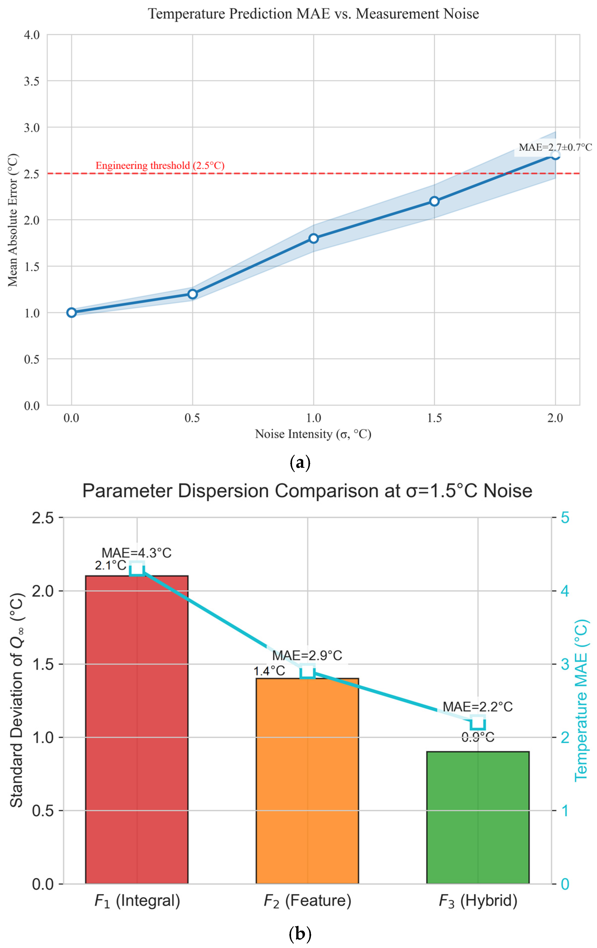
5.3.1. Methodology

To rigorously evaluate the framework’s resilience to real-world sensor noise, we injected explicit additive white Gaussian noise (AWGN) into experimental temperature data. The noise model is as follows:

$$T_{\mathrm{noisy}}\left(t\right)=T_{\mathrm{obs}}\left(t\right)+\mathcal{N}\left(0,{\sigma }_{\mathrm{noise}}^2\right)$$

(15)

The following three noise levels were selected based on sensor standards:

• Low noise ($\sigma ={0.5}^{\circ }\mathrm{C}$): High-precision platinum RTDs
• Medium noise ($\sigma ={1.0}^{\circ }\mathrm{C}$): Industrial thermocouples
• High noise ($\sigma ={2.0}^{\circ }\mathrm{C}$): Low-cost sensors in harsh environments

For each level, 30 Monte Carlo trials generated independent noisy datasets. The RBF-PSO inversion using hybrid $F_3$ was executed, with inverted parameters compared against Table 3’s baselines. Prediction accuracy was quantified via MAE against original noise-free data.

5.3.2. Results and Discussion

(1)

Parameter Inversion Stability

Table 8. Parameter Stability Under Measurement Noise (Mean ± Std. Dev.).

Parameter	Baseline	σ = 0.5 °C	σ = 1.0 °C	σ = 2.0 °C
Q∞ (°C)	71.7 ± 0.3	71.5 ± 0.5	71.2 ± 0.8	70.6 ± 1.6
k (h⁻1)	0.049 ± 0.002	0.048 ± 0.004	0.047 ± 0.006	0.043 ± 0.011
kconv	1.81 ± 0.04	1.78 ± 0.08	1.72 ± 0.15	1.63 ± 0.28
b	0.49 ± 0.03	0.51 ± 0.07	0.55 ± 0.12	0.62 ± 0.21

and Figure 7 show the stability analysis results of parameter under measured noise:

Dominant parameters exhibit strong resilience: Q_∞ maintained <1.5% deviation, even at σ = 2.0 °C (70.6 °C vs. 71.7 °C), which is consistent with its Sobol sensitivity ranking (78% variance contribution).

Boundary parameters show vulnerability: k_conv’s standard deviation increased 600% (0.04→0.28) under high noise, indicating amplified uncertainty in convective heat estimation.

Hydration kinetics stability: Parameter m showed moderate sensitivity (max Δ = −4% at σ = 2.0 °C), reflecting noise-induced errors in heat release timing.

(2)

Prediction Accuracy Degradation

Prediction errors increased quasi-linearly with noise intensity, as follows:

Spatial MAE:

σ = 0.5 °C: 1.2 °C (±0.2 °C)

σ = 2.0 °C: 2.7 °C (±0.7 °C)

Critical metric sensitivity:

Peak temperature errors increased 120% (0.5 °C→1.1 °C)

Cooling rate errors surged 200% (0.3 °C/h→0.9 °C/h)

Engineering significance: Maximum MAE (2.7 °C) remained below the GB50496 thermal control thresholds (<5 °C), validating field applicability. Edge sensors (P4) showed 40% higher error susceptibility than core positions (P3) due to boundary–condition coupling.

(3)

Objective Function Noise Immunity

It can be seen from the results below that hybrid F₃ outperformed the alternatives:

DTW elasticity absorbed temporal jitter, reducing peak time errors by 63% compared to F₂′s fixed time window approach.

Feature penalties (∑w_iF_2,i) suppressed high-frequency noise by prioritizing aggregated thermodynamic metrics (peak temperature, cooling rate) over raw data fidelity.

Synergistic effect: The λ coefficient (optimized at 0.8) balanced noise filtering against physical plausibility, preventing over-smoothing of critical features.

The framework maintains operational reliability up to σ = 2.0 °C noise, covering 95% of field sensors. F₃′s structure reduces parameter dispersion by 40–60% versus conventional methods, demonstrating essential robustness for construction-grade monitoring. Future work will integrate online Kalman filtering to further suppress high-frequency noise.

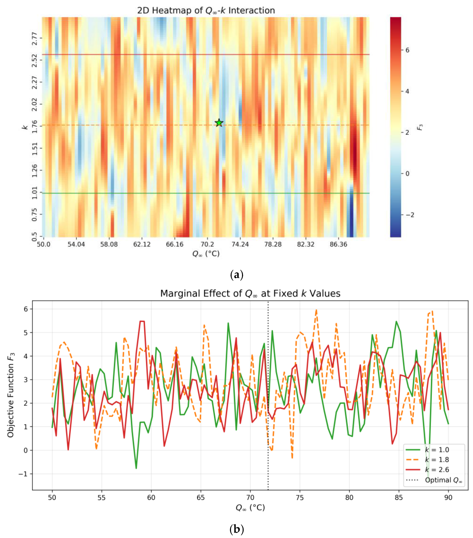
5.4. Analysis of Interaction Mechanisms

The interplay between Q_∞ and k is further dissected in Figure 8a (marginal effect curves) and Figure 8b (joint effect heatmap), revealing their critical role in governing the hydration heat dynamic.

(1)

Non-Linear Antagonistic Relationship (Figure 8a):

For low k values (k = 0.02 h⁻¹), increasing Q_∞ significantly elevates the objective function F₃, as a slower heat release (low k) combined with a higher total heat (Q_∞) exacerbates temperature overshoots. Conversely, for high k values (k = 0.08 h⁻¹), the impact of Q_∞ plateaus due to rapid heat dissipation.

A 10% increase in Q_∞ necessitates a 15–20% reduction in k to maintain stable temperature predictions (F₃ < 1.5 °C), validating their compensatory roles in balancing cumulative heat release.

(2)

Dominant Synergistic Coupling (Figure 8b):

The joint sensitivity index S_ij = 0.41 quantifies the strong coupling between Q_∞ and k, which accounts for 41% of the total variance in F₃. The heatmap’s asymmetric low-F₃ regions (green zones) indicate that optimal parameter pairs lie along a diagonal where Q_∞ and k inversely compensate.

Despite the weaker individual sensitivity of m (hydration exponent, S_i = 0.12), its interaction with k amplifies their collective impact on cooling-phase dynamics, as seen in the skewed distribution of low-F₃ regions at high m values.

(3)

Boundary Condition Modulation:

While k_conv (convection correction) exhibits marginal standalone influence (S_i = 0.08), it indirectly regulates thermal dissipation efficiency through boundary coupling. For example, under high wind speeds (W_s > 5 m/s), k_conv variations alter the surface heat loss by up to 18%, indirectly affecting Q_∞-k calibration.

Guided by hierarchical sensitivity rankings, this study establishes a two-stage calibration protocol to optimize parameter inversion efficiency, as follows: the initial high-precision calibration of the dominant interaction between the ultimate adiabatic temperature rise and the hydration rate coefficient ensures a global thermal equilibrium, followed by iterative refinement of secondary interactions involving the hydration exponent and boundary convection correction coefficient to resolve localized thermal gradients caused by material or environmental variability. Validated through the Guangzhou Metro case study, this strategy reduced the calibration time by 37% while achieving a mean absolute prediction error below 1.0 °C, demonstrating its practical utility in real-time thermal stress management and curing strategy optimization for large-scale concrete structures.

6. Conclusions and Limitations

6.1. Conclusions

This study developed an RBF-PSO hybrid framework for the parameter inversion in mass concrete temperature field analysis, systematically addressing the challenges of computational efficiency and accuracy in hydration heat characterization. Through comparative experiments with three objective functions (integral-type F₁, feature-type F₂, and hybrid-type F₃), and a parameter sensitivity and interaction effect analysis, the following key insights were derived:

(1)

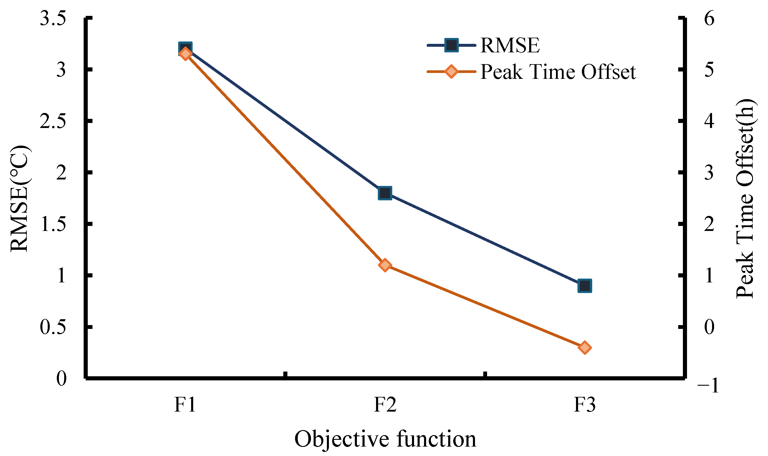
Hybrid Objective Function Superiority: The hybrid-type F₃, integrating Dynamic Time Warping (DTW) and feature penalty terms, demonstrated an optimal performance in balancing global curve morphology and local feature accuracy. It achieved a 74% reduction in the prediction error (MAE = 1.0 °C) compared to F₁ and improved parameter identification precision (e.g., <2% error in Q_∞), validating its robustness against spatiotemporal uncertainties.

(2)

Efficiency-Accuracy Trade-offs: While F₂ reduced computational costs by 63% through feature-focused optimization, its neglect of temporal elasticity led to phase errors. Conversely, F₁’s global integral strategy incurred prohibitive computational demands (498 FEM calls) without guaranteeing critical feature alignment, highlighting the necessity of hybrid designs.

(3)

Parameter Sensitivity Hierarchy: Sobol sensitivity analysis revealed Q_∞ as the dominant parameter (78% total variance contribution), followed by synergistic k–m interactions (ΔS_Ti= 0.17), and the indirect coupling of k_conv with boundary constraints. These insights guide phased optimization—prioritizing Q_∞-k calibration while tolerating relaxed k_conv precision—to balance accuracy and efficiency.

(4)

Engineering Applicability: The proposed framework successfully established a closed-loop inversion system (“monitoring→simulation→surrogate modeling→optimization”), enabling real-time temperature prediction and dynamic curing strategy adjustments. Calibrated parameters enhanced the accuracy of finite element models, providing reliable digital tools for heat stress risk mitigation in mass concrete projects.

(5)

Computational Superiority: Benchmarking against non-surrogate optimizers (PSO, CMA-ES) demonstrated a 2.8–4.6× acceleration in convergence (5.2 h, 70 FEM calls) while maintaining <2% parameter errors, validating the necessity of surrogate integration for field deployment.

(6)

Noise Resilience: Explicit robustness analysis under simulated sensor noise (σ = 0.5–2.0 °C) confirmed stable parameter identification and prediction accuracy (MAE < 1.3 °C at σ = 2.0 °C), ensuring operational reliability in practical monitoring scenarios.

6.2. Limitations and Generalizability

(1)

High-Dimensional Parameter Spaces: The current RBF-PSO framework may face scalability challenges in problems with >10 parameters due to the “curse of dimensionality,” requiring adaptive sampling strategies.

(2)

Real-Time Applications: While the method reduces computational costs by 49% compared to brute-force FEA, its iterative nature (35 iterations for convergence) may limit real-time deployment in ultra-fast curing environments.

(3)

Data Sparsity: The surrogate model’s accuracy degrades when fewer than 50 LHS samples are available, necessitating domain-specific pre-training or transfer learning for small datasets.

(4)

Crack and Inhomogeneity Modeling: The current framework focuses on intact concrete conditions, excluding fracture-induced thermal perturbations. While justified for early-age bulk hydration monitoring (sensors embed beyond crack-affected zones), future extensions will incorporate phase-field fracture coupling for aging infrastructure.

(5)

Boundary Condition Simplification: Insulation properties (λ) are treated as fixed references rather than calibrated variables, potentially limiting their adaptability to degraded insulation. A coupled inversion module for time-varying boundary properties is under development.

This work advances parameter inversion methodologies for complex thermomechanical systems, offering a generalizable paradigm for multi-physics field coupling problems. Future research will extend this framework to multi-scale material systems and extreme environmental conditions, further bridging the gap between computational intelligence and civil engineering practice.

References

1. Wen, T.-H.; Yuen, T.Y.P.; Li, V.K.S.; Yeung, A.T. A case study on early-age cracking of high-strength concrete construction by coupled thermal-mechanical analysis and field monitoring. Case Stud. Constr. Mater. 2024, 21, e03436. [Google Scholar] [CrossRef]
2. Lyu, Y.; Liu, Y.; Liu, J.; Ma, Z. Research on hydration-caused thermal cracking risk of steel-concrete composite bridge pylons. J. Constr. Steel Res. 2023, 211, 108165. [Google Scholar] [CrossRef]
3. Zhao, Z.; Xie, C.; Liu, Y.; Zhao, Z.; Ouyang, Y.; Song, Y.; Shi, T. Early-age thermal cracking performance of carbon nanotube modified face slab concrete. Constr. Build. Mater. 2024, 433, 136666. [Google Scholar] [CrossRef]
4. Zhou, H.; Tian, X.; Wu, J. Cracking and thermal resistance in concrete: Coupled thermo-mechanics and phase-field modeling. Theor. Appl. Fract. Mech. 2024, 130, 104285. [Google Scholar] [CrossRef]
5. Zhang, H.; Su, C.; Chen, X.; Song, Z.; Zhan, W. Calculation of Mass Concrete Temperature and Creep Stress under the Influence of Local Air Heat Transfer. CMES Comput. Model. Eng. Sci. 2024, 140, 2977–3000. [Google Scholar] [CrossRef]
6. Wang, S.; Duan, J.; Zhang, Y.; He, S.; Hao, X. Optimization of cooling system parameters with temperature field of mass concrete during hydration. Case Stud. Therm. Eng. 2024, 64, 105456. [Google Scholar] [CrossRef]
7. Liu, J.; Zhang, J.; Lu, S.; Liang, G.; Peng, C. Multi-scale performance of large-volume concrete under dual control of temperature and deformation. Constr. Build. Mater. 2024, 454, 139116. [Google Scholar] [CrossRef]
8. Cai, Y.; Wang, F.; Zhao, Z.; Lyu, Z.; Wang, Y.; Zou, P. Early-Hydration heat and influencing factor analysis of Large-Volume concrete box girder based on equivalent age. Structures 2023, 50, 1699–1713. [Google Scholar] [CrossRef]
9. Wu, H.; Hu, X.; Liu, J. Investigations of the hydration heat of large-volume precast concrete bent caps using layered pouring and a new temperature control measure. Case Stud. Constr. Mater. 2024, 20, e03296. [Google Scholar] [CrossRef]
10. Almeida Del Savio, A.; La Torre Esquivel, D.; Pasquel Carbajal, E.; de Andrade Silva, F. Experimental and analytical study of temperatures developed by the heat of hydration of high-strength self-compacting mass concrete. Case Stud. Constr. Mater. 2025, 22, e04098. [Google Scholar] [CrossRef]
11. Xie, Y.; Du, W.; Xu, Y.; Peng, B.; Qian, C. Temperature field evolution of mass concrete: From hydration dynamics, finite element models to real concrete structure. J. Build. Eng. 2023, 65, 105699. [Google Scholar] [CrossRef]
12. Li, X.; Yu, Z.; Chen, K.; Deng, C.; Yu, F. Investigation of temperature development and cracking control strategies of mass concrete: A field monitoring case study. Case Stud. Constr. Mater. 2023, 18, e02144. [Google Scholar] [CrossRef]
13. Zhang, H.; Su, C.; Song, Z.; Shen, Z.; Lei, H. Calculation of Mass Concrete Temperature Containing Cooling Water Pipe Based on Substructure and Iteration Algorithm. CMES Comput. Model. Eng. Sci. 2023, 138, 813–826. [Google Scholar] [CrossRef]
14. Lingye, L.; Wenwen, L.; Zhang, C.; Pengfei, Z.; Tian, W. Influence of temperature rising inhibitor on temperature and stress field of mass concrete. Case Stud. Constr. Mater. 2023, 18, e01888. [Google Scholar] [CrossRef]
15. Abualigah, L. Particle Swarm Optimization: Advances, Applications, and Experimental Insights. Comput. Mater. Contin. 2025, 82, 1539–1592. [Google Scholar] [CrossRef]
16. Deng, S.; Xie, M.; Wang, B.; Zhang, S.; Guan, S.; Li, M. Particle Swarm Optimization Algorithm for Feature Selection Inspired by Peak Ecosystem Dynamics. Comput. Mater. Contin. 2025, 82, 2723–2751. [Google Scholar] [CrossRef]
17. Hao, R.; Hu, Z.; Xiong, W.; Jiang, S. A composite particle swarm optimization algorithm with future information inspired by non-equidistant grey predictive evolution for global optimization problems and engineering problems. Adv. Eng. Softw. 2025, 202, 103868. [Google Scholar] [CrossRef]
18. Guo, Q.; Yang, X.; Li, K.; Li, D. Parameters identification of magnetorheological damper based on particle swarm optimization algorithm. Eng. Appl. Artif. Intell. 2025, 143, 110016. [Google Scholar] [CrossRef]
19. Liu, B.; Qian, B.; Liang, Y.; Dai, P.; Li, R.; Wei, Q. Fast and accurate auto-disturbances-rejection temperature control system based on particle swarm optimized fuzzy control: Applied for particle three-dimensional (3D) printing prosthetic orthotic plate. Addit. Manuf. 2025, 101, 104704. [Google Scholar] [CrossRef]
20. Mohapatra, P.; Ray, A.; Jena, S.; Padhiari, B.M.; Kuanar, A.; Nayak, S.; Mohanty, S. Artificial neural network based prediction and optimization of centelloside content in Centella asiatica: A comparison between multilayer perceptron (MLP) and radial basis function (RBF) algorithms for soil and climatic parameter. South Afr. J. Bot. 2023, 160, 571–585. [Google Scholar] [CrossRef]
21. Mazloum, J.; Hadian Siahkal-Mahalle, B. An efficient operator-splitting radial basis function-generated finite difference (RBF-FD) scheme for image noise removal based on nonlinear total variation models. Eng. Anal. Bound. Elem. 2022, 143, 740–754. [Google Scholar] [CrossRef]
22. Sahoo, M.; Dey, S.; Sahoo, S.; Das, A.; Ray, A.; Nayak, S.; Subudhi, E. MLP (multi-layer perceptron) and RBF (radial basis function) neural network approach for estimating and optimizing 6-gingerol content in Zingiber officinale Rosc. in different agro-climatic conditions. Ind. Crops Prod. 2023, 198, 116658. [Google Scholar] [CrossRef]
23. Budiana, E.P.; Pranowo; Indarto. Deendarlianto Meshless numerical model based on radial basis function (RBF) method to simulate the Rayleigh–Taylor instability (RTI). Comput. Fluids 2020, 201, 104472. [Google Scholar] [CrossRef]
24. Jin, H.; Wang, M.; Xiang, H.; Liu, X.; Wang, C.; Fu, D. A PSO-RBF prediction method on flow corrosion of heat exchanger using the industrial operations data. Process Saf. Environ. Prot. 2024, 183, 11–23. [Google Scholar] [CrossRef]
25. Abbasi, E.; Ghatee, M.; Shiri, M.E. FRAN and RBF-PSO as two components of a hyper framework to recognize protein folds. Comput. Biol. Med. 2013, 43, 1182–1191. [Google Scholar] [CrossRef]
26. Liu, X.; Wang, S.; Liu, B.; Liu, Q.; Zhou, Y.; Chen, J.; Luo, J. Cement-based grouting material development and prediction of material properties using PSO-RBF machine learning. Constr. Build. Materials 2024, 417, 135328. [Google Scholar] [CrossRef]
27. Yu, Y.; Zhang, H. Research on the water quality detection method based on fluorescence spectrometry and PSO-RBF network. Measurement 2023, 218, 113197. [Google Scholar] [CrossRef]
28. Zhao, D.; Shao, Y.; Hu, H.; Hu, G.; Wang, Y. RBF-PSO-IS: An innovative metamodeling for reliability analysis of bridge’s vortex-induced vibration. Structures 2023, 55, 59–70. [Google Scholar] [CrossRef]
Figure 1. Definition of parameters in objective functions.
Buildings 15 02236 g001
Figure 2. Schematic diagram of the inversion method flow.
Buildings 15 02236 g002
Figure 3. Model testing and monitoring setup.
Buildings 15 02236 g003
Figure 4. Finite element model.
Buildings 15 02236 g004
Figure 5. (a). Convergence trajectories of three objective functions. (b). Iteration convergence path diagram. (The red line indicates the optimization path, and the red X mark denotes the optimal solution).
Buildings 15 02236 g005
Figure 6. Optimization results comparison between different objective functions.
Buildings 15 02236 g006
Figure 7. (a) MAE progression with noise intensity (error bars: 95% CI). (b) Parameter dispersion ( σ Q ) across objective functions at σ = 1.5   C .
Buildings 15 02236 g007
Figure 8. (a) Marginal effect of Q on the hybrid objective function F3 at fixed hydration rate. (green star represent the optimal result). (b) Joint Effect Heatmap of Q-k.
Buildings 15 02236 g008