


Predictive Models with Applicable Graphical User Interface (GUI) for the Compressive Performance of Quaternary Blended Plastic-Derived Sustainable Mortar

Abstract
1. Introduction
2. Methodology
2.1. Data Collection
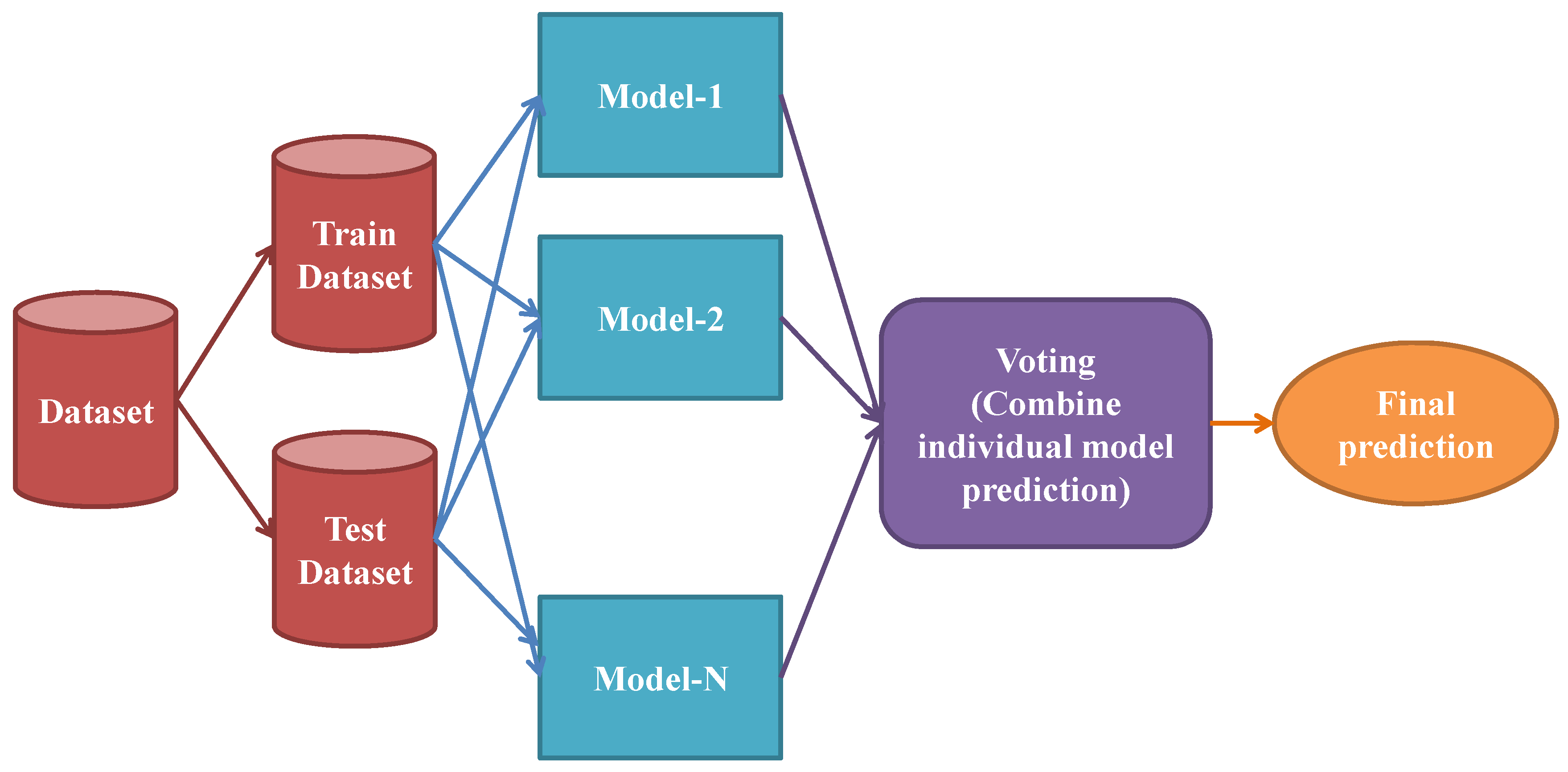
2.2. Machine Learning Modeling
2.2.1. SVM Algorithm
2.2.2. AdaBoost Regressor-ABR
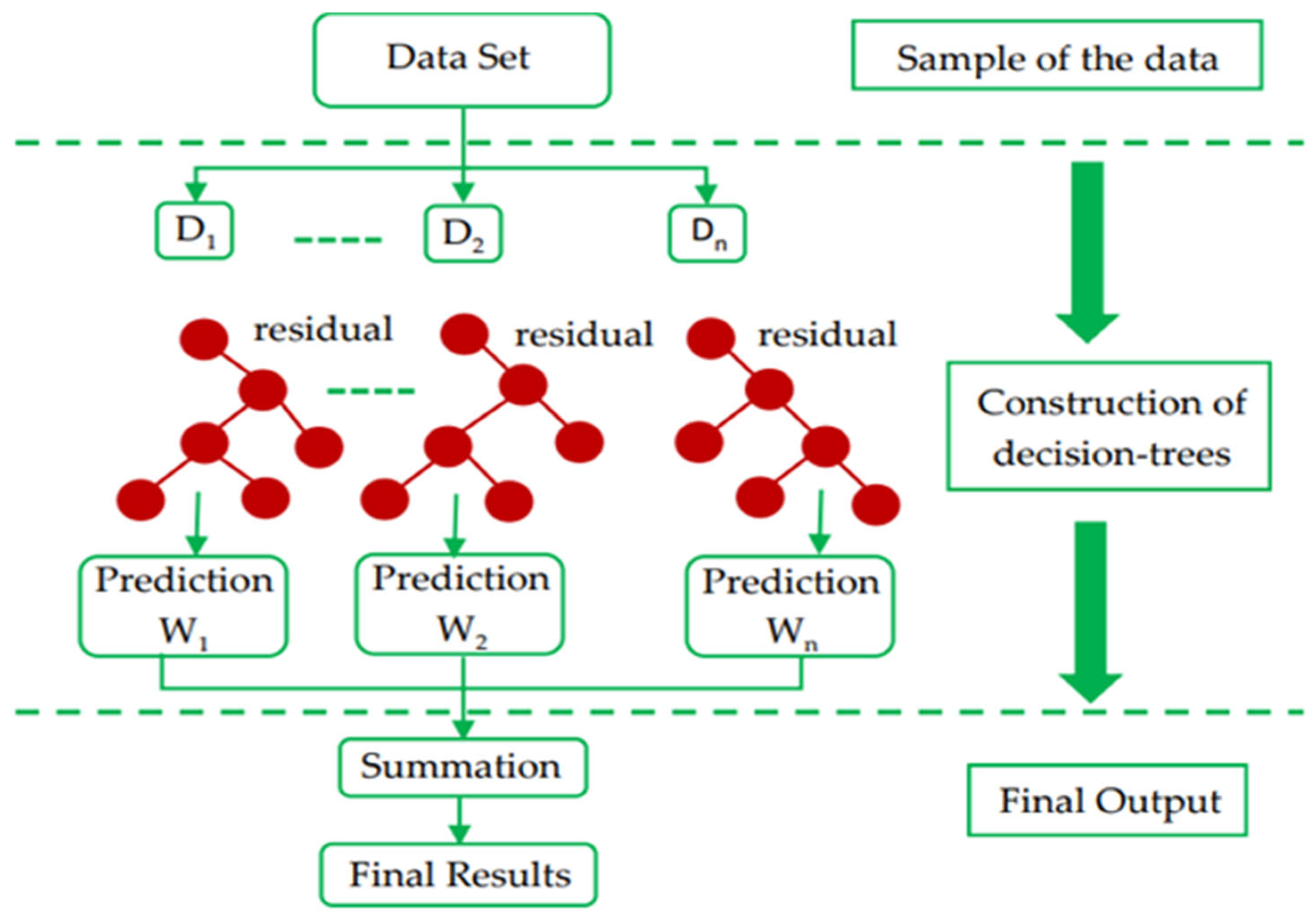
2.2.3. Extreme Gradient Boosting-XGB
2.3. Validation of Models
3. Analysis and Interpretation of Model Results
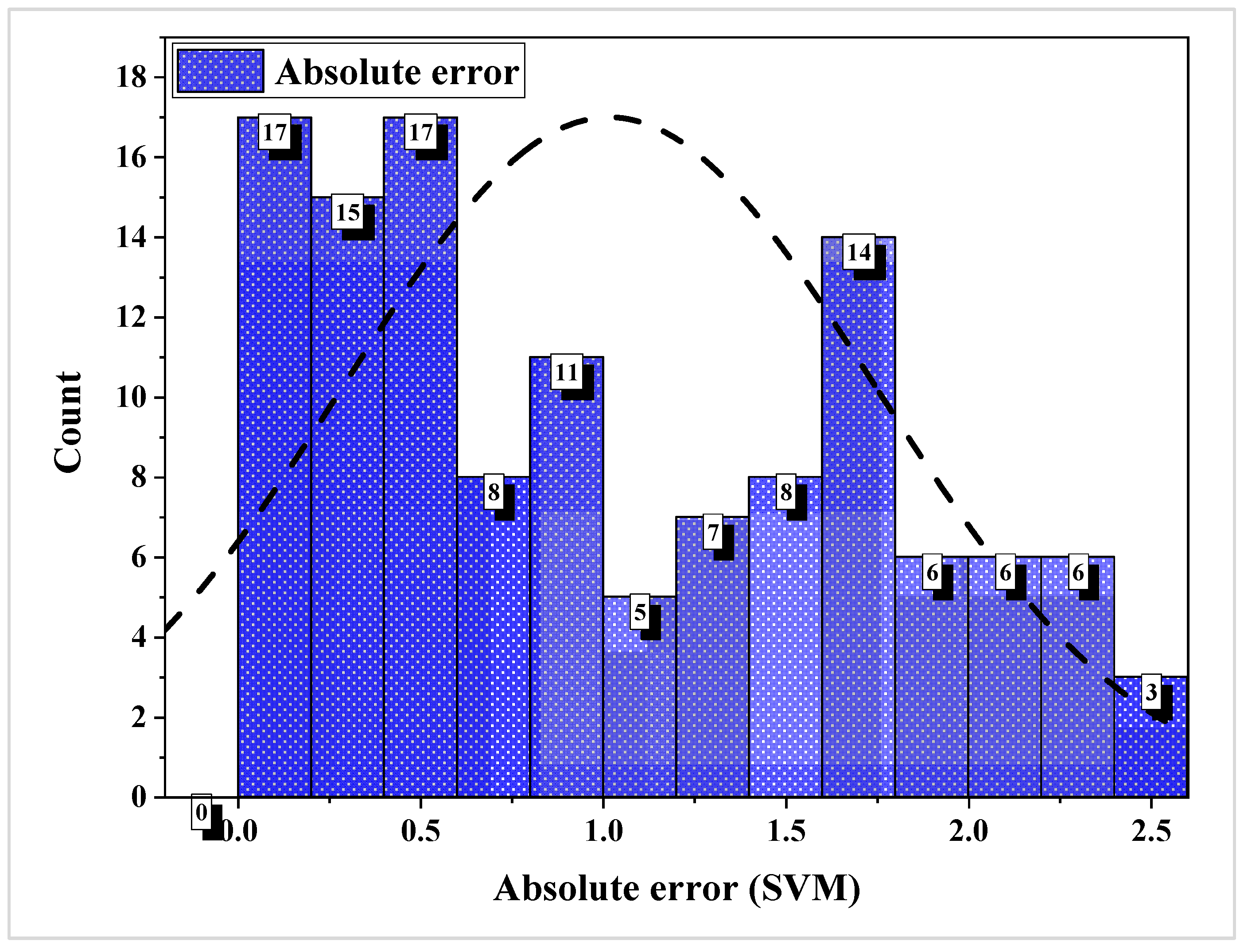
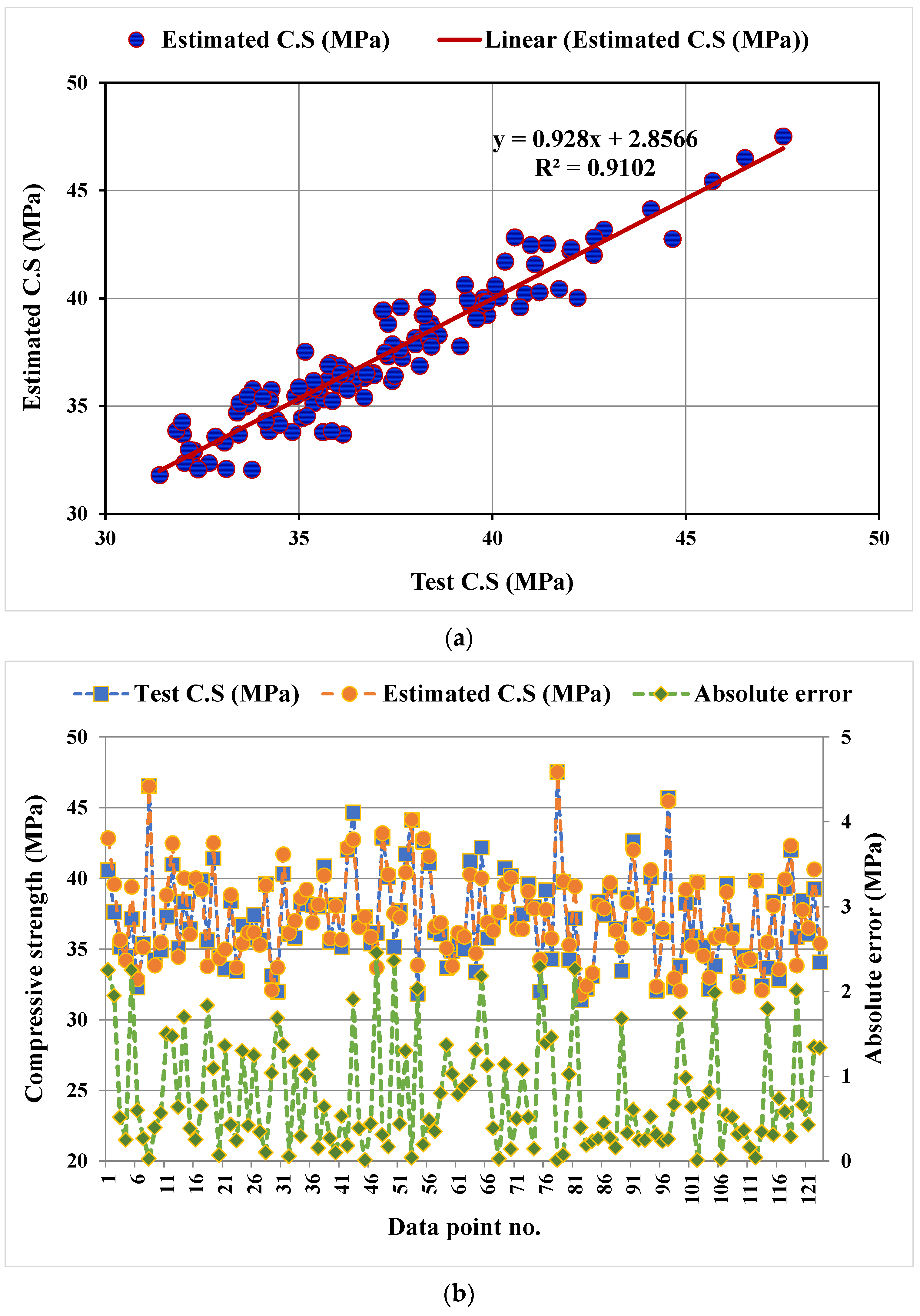
3.1. C.S-SVM Model
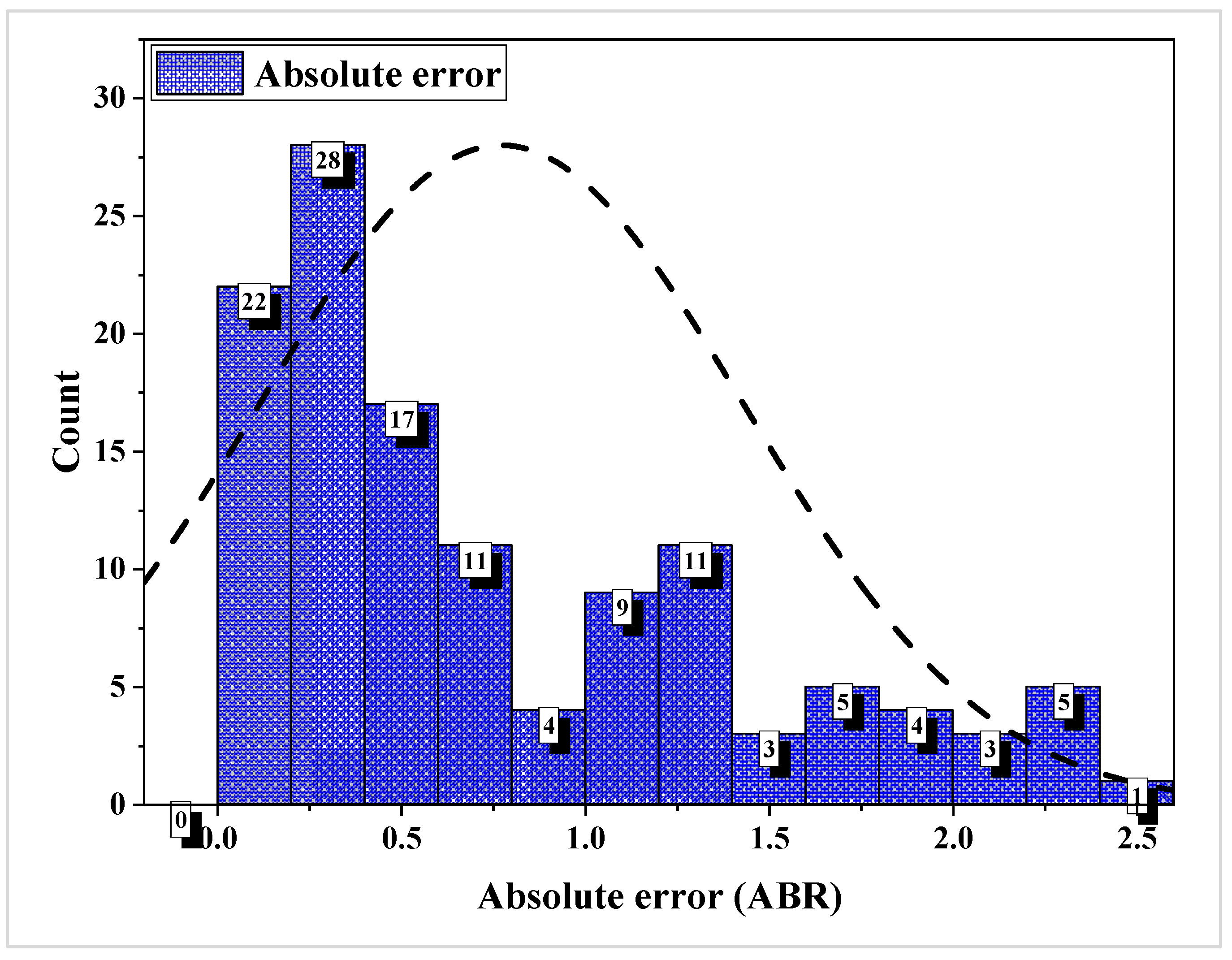
3.2. C.S-ABR Model
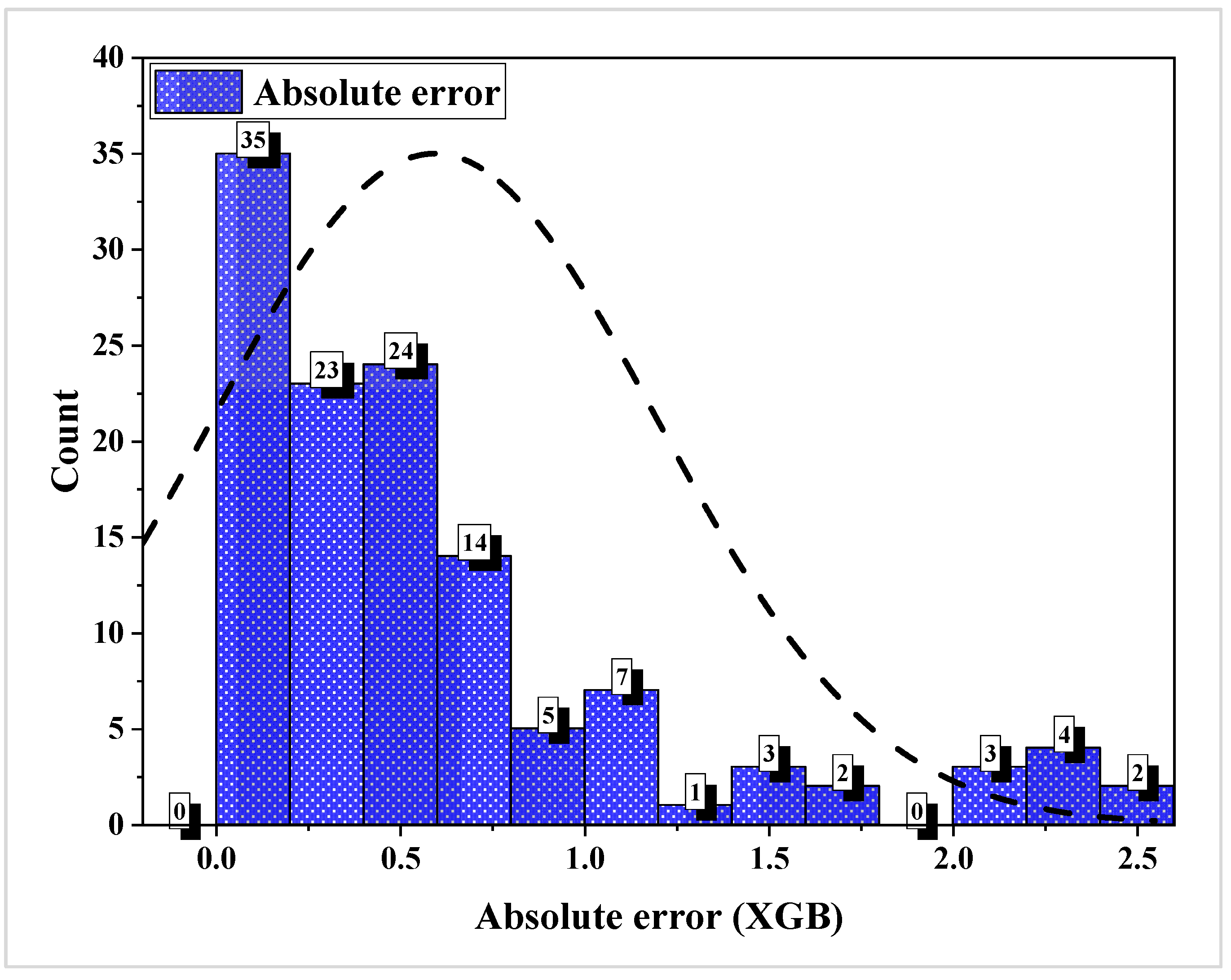
3.3. C.S-XGB Model
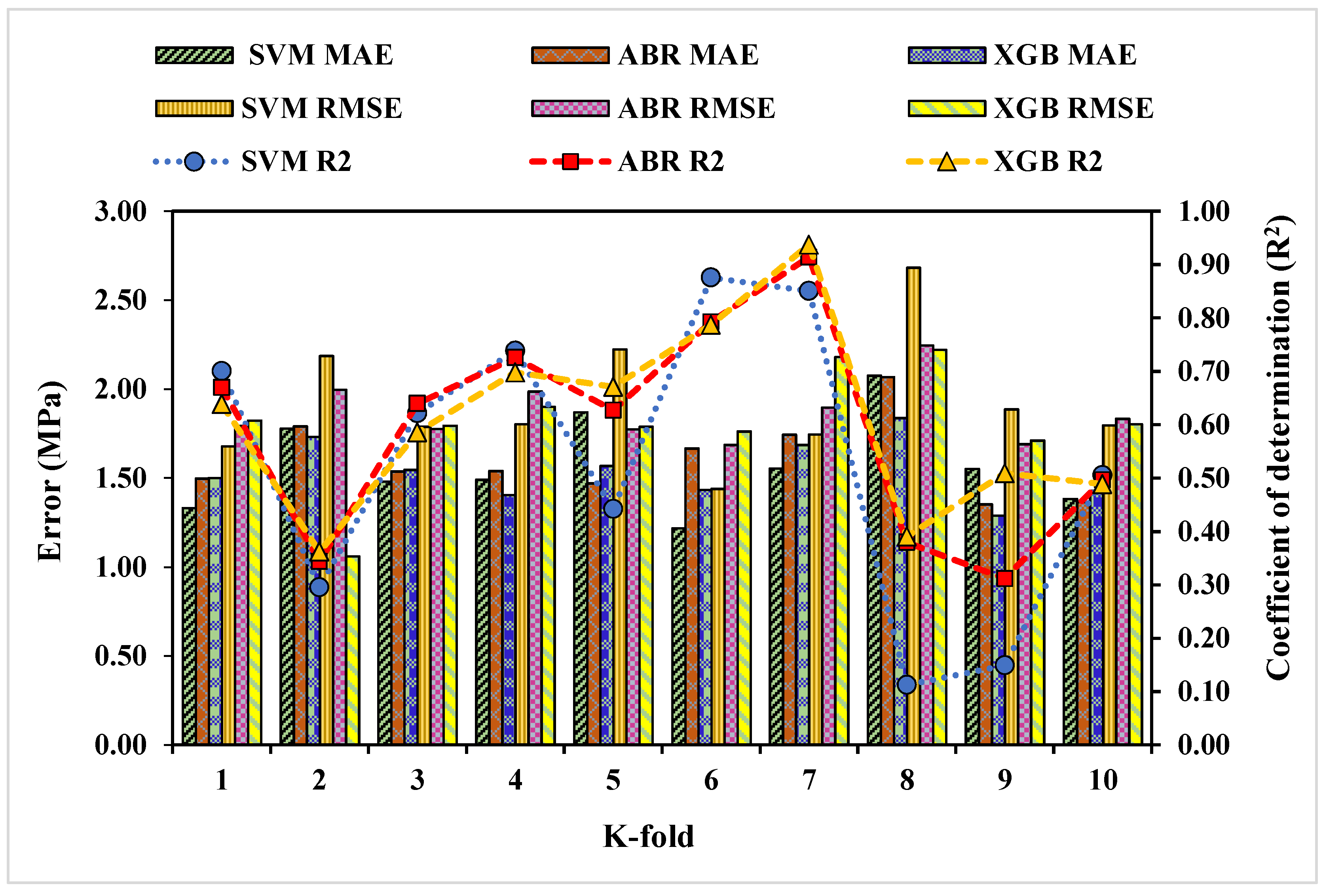
3.4. Model’s Validation Using Statistical and K-Fold Analysis
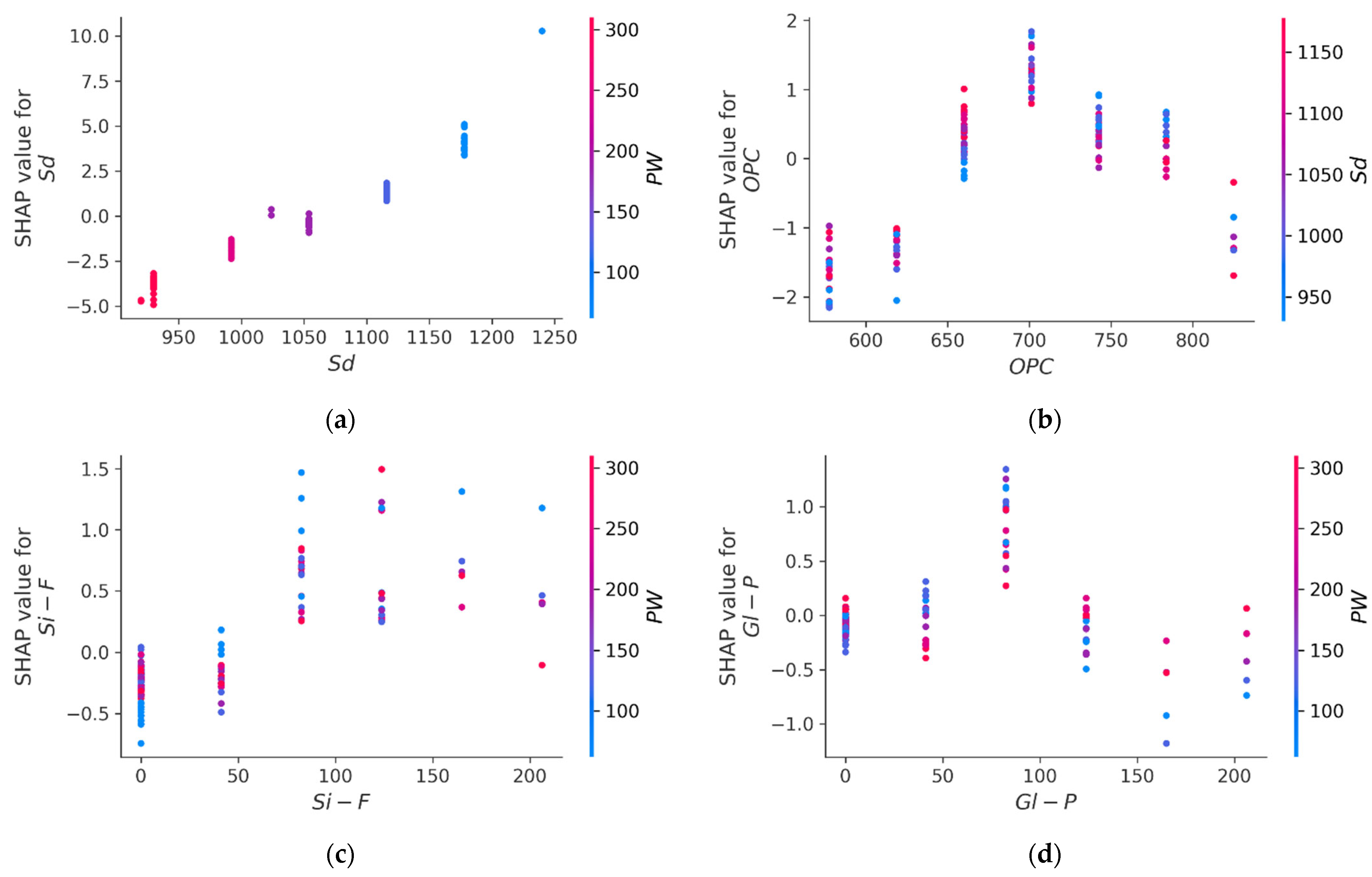
3.5. SHAP Analysis
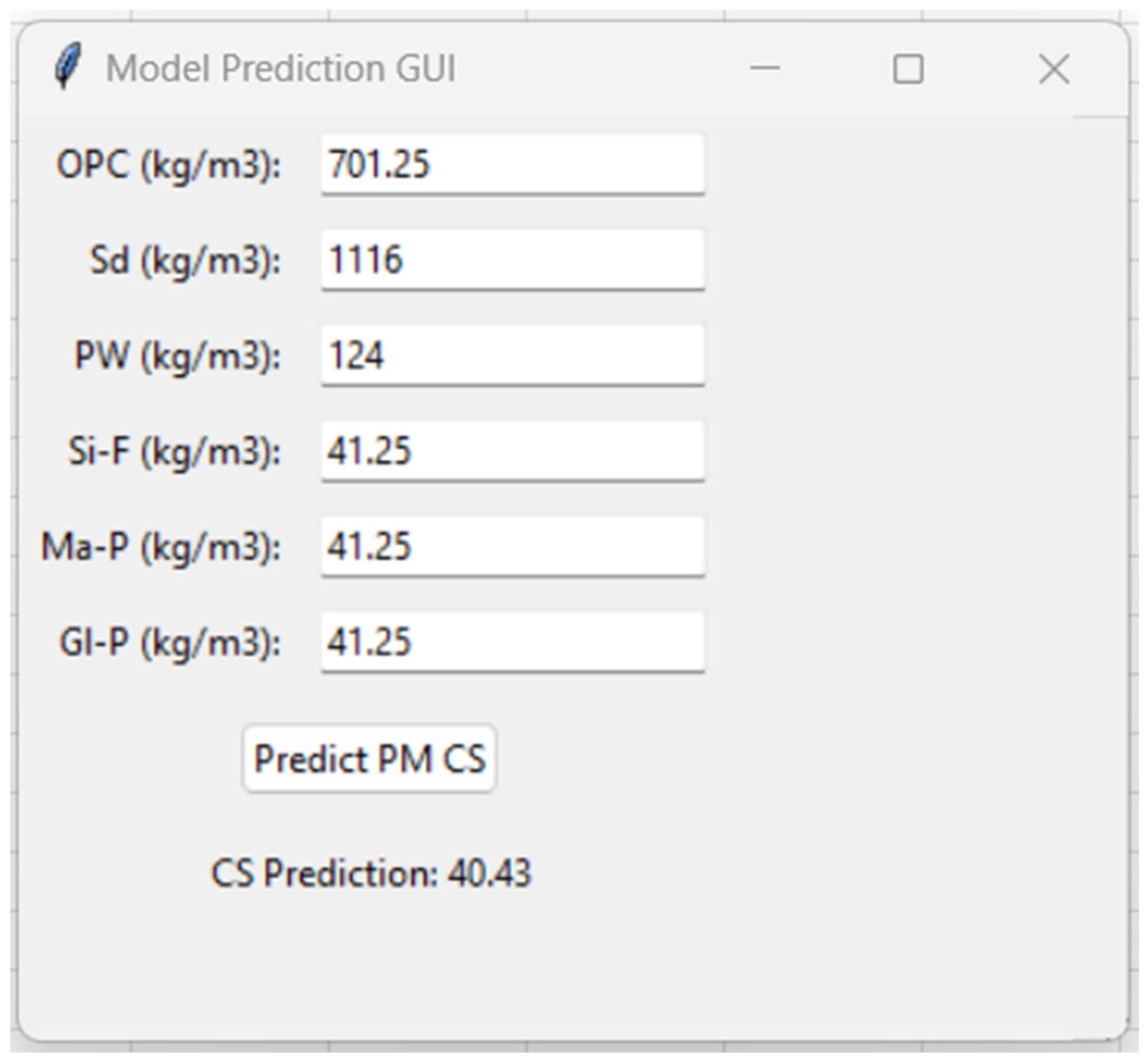
3.6. Graphical User Interface for PMMs Strength
4. Discussions
5. Conclusions
- The XGB method outperformed the ABR and SVM approaches in accurately estimating the C.S of PMMs (R2 = 0.940), while the other two methods achieved R2 values of 0.91 and 0.87, respectively.
- The average difference between the test and forecasted C.S (errors) for the SVM, ABR, and XGB techniques was 1.016 MPa, 0.772 MPa, and 0.592 MPa, respectively. Although the XGB method demonstrated superior accuracy in predicting PMM’s strength, the error levels validated the accuracy of the SVM and ABR models as presented.
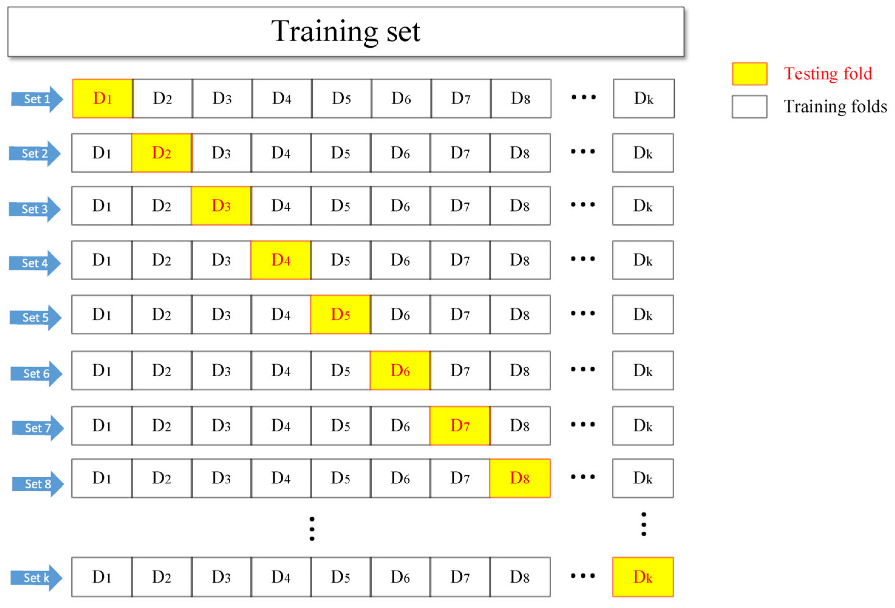
- The effectiveness of the built models was confirmed by statistical and K-fold tests. Improved R2, fewer mistakes, and greater efficiency all point to ML models being accurate. For the C.S prediction, the SVM model had a root mean square error (MAPE) of 2.80%, the ABR model of 2.10%, and the XGB model of 1.60%. According to the MAPE values, the XGB model performed better in predicting the C.S of PMMs.
- The SHAP study found that the PMM’s strength was positively correlated with Sd, OPC, and Si-F, the three primary raw materials and factors. While PW had no effect throughout, Ma-P and Gl-P had a good effect on PMMs strength at the outset but a negative effect as their content increased.
- The created graphical user interface (GUI) is a crucial instrument for predicting the C.S of PMMs, providing a rapid, precise, and intuitive solution that enhances material optimization and encourages sustainable construction practices.
Author Contributions
Funding
Institutional Review Board Statement
Informed Consent Statement
Data Availability Statement
Conflicts of Interest
Correction Statement
Abbreviations
| ABRs | AdaBoost regressors |
| C.S | Compressive strength |
| CBMs | Cement-based materials |
| Gl-P | Glass powder |
| GUI | Graphical user interface |
| Ma-P | Marble powder |
| ML | Machine learning |
| OPC | Ordinary Portland cement |
| PMMs | Plastic-based mortar mixes |
| PW | Plastic |
| R | Pearson correlation |
| R2 | Coefficient of determination |
| SCMs | Supplementary cementitious materials |
| Sd | Sand |
| SHAP | SHapley Additive exPlanations |
| Si-F | Silica fume |
| SVM | Support vector machines pot |
| XGB | Extreme gradient boosting |
Appendix A

| OPC (kg/m3) | Sd (kg/m3) | PW (kg/m3) | Si-F (kg/m3) | Ma-P (kg/m3) | Gl-P (kg/m3) | C.S (MPa) |
|---|---|---|---|---|---|---|
| 825 | 1240 | 0 | 0 | 0 | 0 | 49.29 |
| 825 | 1240 | 0 | 0 | 0 | 0 | 45.7 |
| 825 | 1240 | 0 | 0 | 0 | 0 | 47.2 |
| 825 | 1178 | 62 | 0 | 0 | 0 | 37.13 |
| 825 | 1178 | 62 | 0 | 0 | 0 | 38.2 |
| 825 | 1178 | 62 | 0 | 0 | 0 | 39.87 |
| 825 | 1116 | 124 | 0 | 0 | 0 | 35.38 |
| 825 | 1116 | 124 | 0 | 0 | 0 | 37.41 |
| 825 | 1116 | 124 | 0 | 0 | 0 | 38.01 |
| 825 | 1054 | 186 | 0 | 0 | 0 | 32.49 |
| 825 | 1054 | 186 | 0 | 0 | 0 | 38.37 |
| 825 | 1054 | 186 | 0 | 0 | 0 | 36.14 |
| 825 | 992 | 248 | 0 | 0 | 0 | 36.21 |
| 825 | 992 | 248 | 0 | 0 | 0 | 31.84 |
| 825 | 992 | 248 | 0 | 0 | 0 | 35.07 |
| 825 | 930 | 310 | 0 | 0 | 0 | 33.45 |
| 825 | 930 | 310 | 0 | 0 | 0 | 35.03 |
| 825 | 930 | 310 | 0 | 0 | 0 | 29.95 |
| 783.75 | 1178 | 62 | 41.25 | 0 | 0 | 44.32 |
| 783.75 | 1178 | 62 | 41.25 | 0 | 0 | 40.21 |
| 783.75 | 1178 | 62 | 41.25 | 0 | 0 | 42.02 |
| 742.5 | 1178 | 62 | 82.5 | 0 | 0 | 43.35 |
| 742.5 | 1178 | 62 | 82.5 | 0 | 0 | 46.53 |
| 742.5 | 1178 | 62 | 82.5 | 0 | 0 | 42.01 |
| 701.25 | 1178 | 62 | 123.75 | 0 | 0 | 42.91 |
| 701.25 | 1178 | 62 | 123.75 | 0 | 0 | 44.68 |
| 701.25 | 1178 | 62 | 123.75 | 0 | 0 | 47.52 |
| 660 | 1178 | 62 | 165 | 0 | 0 | 43.69 |
| 660 | 1178 | 62 | 165 | 0 | 0 | 46.39 |
| 660 | 1178 | 62 | 165 | 0 | 0 | 44.31 |
| 618.75 | 1178 | 62 | 206.25 | 0 | 0 | 46.05 |
| 618.75 | 1178 | 62 | 206.25 | 0 | 0 | 44.21 |
| 618.75 | 1178 | 62 | 206.25 | 0 | 0 | 41.64 |
| 783.75 | 1116 | 124 | 41.25 | 0 | 0 | 38.63 |
| 783.75 | 1116 | 124 | 41.25 | 0 | 0 | 35.48 |
| 783.75 | 1116 | 124 | 41.25 | 0 | 0 | 40.26 |
| 742.5 | 1116 | 124 | 82.5 | 0 | 0 | 42.17 |
| 742.5 | 1116 | 124 | 82.5 | 0 | 0 | 39.36 |
| 742.5 | 1116 | 124 | 82.5 | 0 | 0 | 36.75 |
| 701.25 | 1116 | 124 | 123.75 | 0 | 0 | 43.56 |
| 701.25 | 1116 | 124 | 123.75 | 0 | 0 | 38.83 |
| 701.25 | 1116 | 124 | 123.75 | 0 | 0 | 42.62 |
| 660 | 1116 | 124 | 165 | 0 | 0 | 38.54 |
| 660 | 1116 | 124 | 165 | 0 | 0 | 40.65 |
| 660 | 1116 | 124 | 165 | 0 | 0 | 41.79 |
| 618.75 | 1116 | 124 | 206.25 | 0 | 0 | 38.41 |
| 618.75 | 1116 | 124 | 206.25 | 0 | 0 | 39.79 |
| 618.75 | 1116 | 124 | 206.25 | 0 | 0 | 34.75 |
| 783.75 | 1054 | 186 | 41.25 | 0 | 0 | 38.46 |
| 783.75 | 1054 | 186 | 41.25 | 0 | 0 | 37.77 |
| 783.75 | 1054 | 186 | 41.25 | 0 | 0 | 34.76 |
| 742.5 | 1054 | 186 | 82.5 | 0 | 0 | 39.74 |
| 742.5 | 1054 | 186 | 82.5 | 0 | 0 | 37.18 |
| 742.5 | 1054 | 186 | 82.5 | 0 | 0 | 38.03 |
| 701.25 | 1054 | 186 | 123.75 | 0 | 0 | 39.77 |
| 701.25 | 1054 | 186 | 123.75 | 0 | 0 | 38.32 |
| 701.25 | 1054 | 186 | 123.75 | 0 | 0 | 42.2 |
| 660 | 1054 | 186 | 165 | 0 | 0 | 40.91 |
| 660 | 1054 | 186 | 165 | 0 | 0 | 36.23 |
| 660 | 1054 | 186 | 165 | 0 | 0 | 37.31 |
| 618.75 | 1054 | 186 | 206.25 | 0 | 0 | 36.42 |
| 618.75 | 1054 | 186 | 206.25 | 0 | 0 | 37.11 |
| 618.75 | 1054 | 186 | 206.25 | 0 | 0 | 35.13 |
| 783.75 | 992 | 248 | 41.25 | 0 | 0 | 36.45 |
| 783.75 | 992 | 248 | 41.25 | 0 | 0 | 36.68 |
| 783.75 | 992 | 248 | 41.25 | 0 | 0 | 34.14 |
| 742.5 | 992 | 248 | 82.5 | 0 | 0 | 38.96 |
| 742.5 | 992 | 248 | 82.5 | 0 | 0 | 37.42 |
| 742.5 | 992 | 248 | 82.5 | 0 | 0 | 35.15 |
| 701.25 | 992 | 248 | 123.75 | 0 | 0 | 38.5 |
| 701.25 | 992 | 248 | 123.75 | 0 | 0 | 37.61 |
| 701.25 | 992 | 248 | 123.75 | 0 | 0 | 40.94 |
| 660 | 992 | 248 | 165 | 0 | 0 | 32.87 |
| 660 | 992 | 248 | 165 | 0 | 0 | 36.29 |
| 660 | 992 | 248 | 165 | 0 | 0 | 37.48 |
| 618.75 | 992 | 248 | 206.25 | 0 | 0 | 34.23 |
| 618.75 | 992 | 248 | 206.25 | 0 | 0 | 35.85 |
| 618.75 | 992 | 248 | 206.25 | 0 | 0 | 33.12 |
| 783.75 | 930 | 310 | 41.25 | 0 | 0 | 33.62 |
| 783.75 | 930 | 310 | 41.25 | 0 | 0 | 35.53 |
| 783.75 | 930 | 310 | 41.25 | 0 | 0 | 33.2 |
| 742.5 | 930 | 310 | 82.5 | 0 | 0 | 33.81 |
| 742.5 | 930 | 310 | 82.5 | 0 | 0 | 35.39 |
| 742.5 | 930 | 310 | 82.5 | 0 | 0 | 38.2 |
| 701.25 | 930 | 310 | 123.75 | 0 | 0 | 39.31 |
| 701.25 | 930 | 310 | 123.75 | 0 | 0 | 36.78 |
| 701.25 | 930 | 310 | 123.75 | 0 | 0 | 35.88 |
| 660 | 930 | 310 | 165 | 0 | 0 | 32.47 |
| 660 | 930 | 310 | 165 | 0 | 0 | 34.49 |
| 660 | 930 | 310 | 165 | 0 | 0 | 31.98 |
| 618.75 | 930 | 310 | 206.25 | 0 | 0 | 33.12 |
| 618.75 | 930 | 310 | 206.25 | 0 | 0 | 31.25 |
| 618.75 | 930 | 310 | 206.25 | 0 | 0 | 29.65 |
| 783.75 | 1178 | 62 | 0 | 41.25 | 0 | 41.21 |
| 783.75 | 1178 | 62 | 0 | 41.25 | 0 | 40.09 |
| 783.75 | 1178 | 62 | 0 | 41.25 | 0 | 38.25 |
| 742.5 | 1178 | 62 | 0 | 82.5 | 0 | 39.58 |
| 742.5 | 1178 | 62 | 0 | 82.5 | 0 | 41.73 |
| 742.5 | 1178 | 62 | 0 | 82.5 | 0 | 42 |
| 701.25 | 1178 | 62 | 0 | 123.75 | 0 | 43.23 |
| 701.25 | 1178 | 62 | 0 | 123.75 | 0 | 44.1 |
| 701.25 | 1178 | 62 | 0 | 123.75 | 0 | 39.12 |
| 660 | 1178 | 62 | 0 | 165 | 0 | 42.62 |
| 660 | 1178 | 62 | 0 | 165 | 0 | 39.17 |
| 660 | 1178 | 62 | 0 | 165 | 0 | 38.43 |
| 618.75 | 1178 | 62 | 0 | 206.25 | 0 | 37.57 |
| 618.75 | 1178 | 62 | 0 | 206.25 | 0 | 39.17 |
| 618.75 | 1178 | 62 | 0 | 206.25 | 0 | 40.11 |
| 783.75 | 1116 | 124 | 0 | 41.25 | 0 | 38.28 |
| 783.75 | 1116 | 124 | 0 | 41.25 | 0 | 39.69 |
| 783.75 | 1116 | 124 | 0 | 41.25 | 0 | 35.82 |
| 742.5 | 1116 | 124 | 0 | 82.5 | 0 | 38.89 |
| 742.5 | 1116 | 124 | 0 | 82.5 | 0 | 37.38 |
| 742.5 | 1116 | 124 | 0 | 82.5 | 0 | 40.85 |
| 701.25 | 1116 | 124 | 0 | 123.75 | 0 | 41.15 |
| 701.25 | 1116 | 124 | 0 | 123.75 | 0 | 40.86 |
| 701.25 | 1116 | 124 | 0 | 123.75 | 0 | 38.77 |
| 660 | 1116 | 124 | 0 | 165 | 0 | 37.58 |
| 660 | 1116 | 124 | 0 | 165 | 0 | 39.54 |
| 660 | 1116 | 124 | 0 | 165 | 0 | 38.51 |
| 618.75 | 1116 | 124 | 0 | 206.25 | 0 | 37.72 |
| 618.75 | 1116 | 124 | 0 | 206.25 | 0 | 38.2 |
| 618.75 | 1116 | 124 | 0 | 206.25 | 0 | 35.16 |
| 783.75 | 1054 | 186 | 0 | 41.25 | 0 | 37.52 |
| 783.75 | 1054 | 186 | 0 | 41.25 | 0 | 36.24 |
| 783.75 | 1054 | 186 | 0 | 41.25 | 0 | 34.25 |
| 742.5 | 1054 | 186 | 0 | 82.5 | 0 | 36.75 |
| 742.5 | 1054 | 186 | 0 | 82.5 | 0 | 35.78 |
| 742.5 | 1054 | 186 | 0 | 82.5 | 0 | 38.23 |
| 701.25 | 1054 | 186 | 0 | 123.75 | 0 | 38.79 |
| 701.25 | 1054 | 186 | 0 | 123.75 | 0 | 39.33 |
| 701.25 | 1054 | 186 | 0 | 123.75 | 0 | 36.19 |
| 660 | 1054 | 186 | 0 | 165 | 0 | 35.65 |
| 660 | 1054 | 186 | 0 | 165 | 0 | 34.9 |
| 660 | 1054 | 186 | 0 | 165 | 0 | 37.3 |
| 618.75 | 1054 | 186 | 0 | 206.25 | 0 | 33.79 |
| 618.75 | 1054 | 186 | 0 | 206.25 | 0 | 34.46 |
| 618.75 | 1054 | 186 | 0 | 206.25 | 0 | 37.35 |
| 783.75 | 992 | 248 | 0 | 41.25 | 0 | 37.02 |
| 783.75 | 992 | 248 | 0 | 41.25 | 0 | 34.72 |
| 783.75 | 992 | 248 | 0 | 41.25 | 0 | 34.25 |
| 742.5 | 992 | 248 | 0 | 82.5 | 0 | 34.29 |
| 742.5 | 992 | 248 | 0 | 82.5 | 0 | 36.26 |
| 742.5 | 992 | 248 | 0 | 82.5 | 0 | 37.8 |
| 701.25 | 992 | 248 | 0 | 123.75 | 0 | 37.61 |
| 701.25 | 992 | 248 | 0 | 123.75 | 0 | 38.34 |
| 701.25 | 992 | 248 | 0 | 123.75 | 0 | 35.12 |
| 660 | 992 | 248 | 0 | 165 | 0 | 37.92 |
| 660 | 992 | 248 | 0 | 165 | 0 | 34.86 |
| 660 | 992 | 248 | 0 | 165 | 0 | 33.14 |
| 618.75 | 992 | 248 | 0 | 206.25 | 0 | 34.83 |
| 618.75 | 992 | 248 | 0 | 206.25 | 0 | 35.4 |
| 618.75 | 992 | 248 | 0 | 206.25 | 0 | 32.49 |
| 783.75 | 930 | 310 | 0 | 41.25 | 0 | 35.62 |
| 783.75 | 930 | 310 | 0 | 41.25 | 0 | 33.32 |
| 783.75 | 930 | 310 | 0 | 41.25 | 0 | 31.4 |
| 742.5 | 930 | 310 | 0 | 82.5 | 0 | 35.07 |
| 742.5 | 930 | 310 | 0 | 82.5 | 0 | 32 |
| 742.5 | 930 | 310 | 0 | 82.5 | 0 | 36.14 |
| 701.25 | 930 | 310 | 0 | 123.75 | 0 | 37.67 |
| 701.25 | 930 | 310 | 0 | 123.75 | 0 | 34.47 |
| 701.25 | 930 | 310 | 0 | 123.75 | 0 | 33.78 |
| 660 | 930 | 310 | 0 | 165 | 0 | 28.56 |
| 660 | 930 | 310 | 0 | 165 | 0 | 32.69 |
| 660 | 930 | 310 | 0 | 165 | 0 | 32.08 |
| 618.75 | 930 | 310 | 0 | 206.25 | 0 | 31.66 |
| 618.75 | 930 | 310 | 0 | 206.25 | 0 | 29.42 |
| 618.75 | 930 | 310 | 0 | 206.25 | 0 | 34.91 |
| 783.75 | 1178 | 62 | 0 | 0 | 41.25 | 39.6 |
| 783.75 | 1178 | 62 | 0 | 0 | 41.25 | 42.23 |
| 783.75 | 1178 | 62 | 0 | 0 | 41.25 | 40.68 |
| 742.5 | 1178 | 62 | 0 | 0 | 82.5 | 42.89 |
| 742.5 | 1178 | 62 | 0 | 0 | 82.5 | 44.05 |
| 742.5 | 1178 | 62 | 0 | 0 | 82.5 | 41.2 |
| 701.25 | 1178 | 62 | 0 | 0 | 123.75 | 43.54 |
| 701.25 | 1178 | 62 | 0 | 0 | 123.75 | 41.42 |
| 701.25 | 1178 | 62 | 0 | 0 | 123.75 | 39.61 |
| 660 | 1178 | 62 | 0 | 0 | 165 | 38.91 |
| 660 | 1178 | 62 | 0 | 0 | 165 | 39.87 |
| 660 | 1178 | 62 | 0 | 0 | 165 | 41.73 |
| 618.75 | 1178 | 62 | 0 | 0 | 206.25 | 37 |
| 618.75 | 1178 | 62 | 0 | 0 | 206.25 | 41.78 |
| 618.75 | 1178 | 62 | 0 | 0 | 206.25 | 37.54 |
| 783.75 | 1116 | 124 | 0 | 0 | 41.25 | 40.15 |
| 783.75 | 1116 | 124 | 0 | 0 | 41.25 | 38.48 |
| 783.75 | 1116 | 124 | 0 | 0 | 41.25 | 36.14 |
| 742.5 | 1116 | 124 | 0 | 0 | 82.5 | 41.29 |
| 742.5 | 1116 | 124 | 0 | 0 | 82.5 | 42.53 |
| 742.5 | 1116 | 124 | 0 | 0 | 82.5 | 38.81 |
| 701.25 | 1116 | 124 | 0 | 0 | 123.75 | 40.39 |
| 701.25 | 1116 | 124 | 0 | 0 | 123.75 | 39.62 |
| 701.25 | 1116 | 124 | 0 | 0 | 123.75 | 38.29 |
| 660 | 1116 | 124 | 0 | 0 | 165 | 35.48 |
| 660 | 1116 | 124 | 0 | 0 | 165 | 37.73 |
| 660 | 1116 | 124 | 0 | 0 | 165 | 38.42 |
| 618.75 | 1116 | 124 | 0 | 0 | 206.25 | 34.91 |
| 618.75 | 1116 | 124 | 0 | 0 | 206.25 | 35.87 |
| 618.75 | 1116 | 124 | 0 | 0 | 206.25 | 38.98 |
| 783.75 | 1054 | 186 | 0 | 0 | 41.25 | 37.45 |
| 783.75 | 1054 | 186 | 0 | 0 | 41.25 | 38.92 |
| 783.75 | 1054 | 186 | 0 | 0 | 41.25 | 35.26 |
| 742.5 | 1054 | 186 | 0 | 0 | 82.5 | 36.74 |
| 742.5 | 1054 | 186 | 0 | 0 | 82.5 | 37.68 |
| 742.5 | 1054 | 186 | 0 | 0 | 82.5 | 41.26 |
| 701.25 | 1054 | 186 | 0 | 0 | 123.75 | 37.67 |
| 701.25 | 1054 | 186 | 0 | 0 | 123.75 | 35.38 |
| 701.25 | 1054 | 186 | 0 | 0 | 123.75 | 38.45 |
| 660 | 1054 | 186 | 0 | 0 | 165 | 35.34 |
| 660 | 1054 | 186 | 0 | 0 | 165 | 36.28 |
| 660 | 1054 | 186 | 0 | 0 | 165 | 38.83 |
| 618.75 | 1054 | 186 | 0 | 0 | 206.25 | 37.2 |
| 618.75 | 1054 | 186 | 0 | 0 | 206.25 | 35.21 |
| 618.75 | 1054 | 186 | 0 | 0 | 206.25 | 33.88 |
| 783.75 | 992 | 248 | 0 | 0 | 41.25 | 34.69 |
| 783.75 | 992 | 248 | 0 | 0 | 41.25 | 35.74 |
| 783.75 | 992 | 248 | 0 | 0 | 41.25 | 37.27 |
| 742.5 | 992 | 248 | 0 | 0 | 82.5 | 39.6 |
| 742.5 | 992 | 248 | 0 | 0 | 82.5 | 36.64 |
| 742.5 | 992 | 248 | 0 | 0 | 82.5 | 35.82 |
| 701.25 | 992 | 248 | 0 | 0 | 123.75 | 35.78 |
| 701.25 | 992 | 248 | 0 | 0 | 123.75 | 35.58 |
| 701.25 | 992 | 248 | 0 | 0 | 123.75 | 38.6 |
| 660 | 992 | 248 | 0 | 0 | 165 | 34.79 |
| 660 | 992 | 248 | 0 | 0 | 165 | 35.64 |
| 660 | 992 | 248 | 0 | 0 | 165 | 37.08 |
| 618.75 | 992 | 248 | 0 | 0 | 206.25 | 33.57 |
| 618.75 | 992 | 248 | 0 | 0 | 206.25 | 35 |
| 618.75 | 992 | 248 | 0 | 0 | 206.25 | 34.73 |
| 783.75 | 930 | 310 | 0 | 0 | 41.25 | 35.82 |
| 783.75 | 930 | 310 | 0 | 0 | 41.25 | 32.28 |
| 783.75 | 930 | 310 | 0 | 0 | 41.25 | 33.83 |
| 742.5 | 930 | 310 | 0 | 0 | 82.5 | 33.68 |
| 742.5 | 930 | 310 | 0 | 0 | 82.5 | 35.63 |
| 742.5 | 930 | 310 | 0 | 0 | 82.5 | 36.93 |
| 701.25 | 930 | 310 | 0 | 0 | 123.75 | 36.69 |
| 701.25 | 930 | 310 | 0 | 0 | 123.75 | 34.06 |
| 701.25 | 930 | 310 | 0 | 0 | 123.75 | 32.21 |
| 660 | 930 | 310 | 0 | 0 | 165 | 31.32 |
| 660 | 930 | 310 | 0 | 0 | 165 | 33.4 |
| 660 | 930 | 310 | 0 | 0 | 165 | 35.38 |
| 618.75 | 930 | 310 | 0 | 0 | 206.25 | 31.41 |
| 618.75 | 930 | 310 | 0 | 0 | 206.25 | 32.84 |
| 618.75 | 930 | 310 | 0 | 0 | 206.25 | 34.24 |
| 742.5 | 1178 | 62 | 41.25 | 41.25 | 0 | 42.95 |
| 742.5 | 1178 | 62 | 41.25 | 41.25 | 0 | 40.36 |
| 742.5 | 1178 | 62 | 41.25 | 41.25 | 0 | 40.22 |
| 660 | 1178 | 62 | 82.5 | 82.5 | 0 | 41 |
| 660 | 1178 | 62 | 82.5 | 82.5 | 0 | 44.17 |
| 660 | 1178 | 62 | 82.5 | 82.5 | 0 | 43.7 |
| 577.5 | 1178 | 62 | 123.75 | 123.75 | 0 | 41.37 |
| 577.5 | 1178 | 62 | 123.75 | 123.75 | 0 | 39.26 |
| 577.5 | 1178 | 62 | 123.75 | 123.75 | 0 | 37.32 |
| 742.5 | 1116 | 124 | 41.25 | 41.25 | 0 | 36.08 |
| 742.5 | 1116 | 124 | 41.25 | 41.25 | 0 | 36.75 |
| 742.5 | 1116 | 124 | 41.25 | 41.25 | 0 | 38.54 |
| 660 | 1116 | 124 | 82.5 | 82.5 | 0 | 40.08 |
| 660 | 1116 | 124 | 82.5 | 82.5 | 0 | 41 |
| 660 | 1116 | 124 | 82.5 | 82.5 | 0 | 38.72 |
| 577.5 | 1116 | 124 | 123.75 | 123.75 | 0 | 35.71 |
| 577.5 | 1116 | 124 | 123.75 | 123.75 | 0 | 37.54 |
| 577.5 | 1116 | 124 | 123.75 | 123.75 | 0 | 39.63 |
| 742.5 | 1054 | 186 | 41.25 | 41.25 | 0 | 36.09 |
| 742.5 | 1054 | 186 | 41.25 | 41.25 | 0 | 38.82 |
| 742.5 | 1054 | 186 | 41.25 | 41.25 | 0 | 34.5 |
| 660 | 1054 | 186 | 82.5 | 82.5 | 0 | 36.92 |
| 660 | 1054 | 186 | 82.5 | 82.5 | 0 | 37.04 |
| 660 | 1054 | 186 | 82.5 | 82.5 | 0 | 40.2 |
| 577.5 | 1054 | 186 | 123.75 | 123.75 | 0 | 37.54 |
| 577.5 | 1054 | 186 | 123.75 | 123.75 | 0 | 36.01 |
| 577.5 | 1054 | 186 | 123.75 | 123.75 | 0 | 33.58 |
| 742.5 | 992 | 248 | 41.25 | 41.25 | 0 | 33.71 |
| 742.5 | 992 | 248 | 41.25 | 41.25 | 0 | 34.17 |
| 742.5 | 992 | 248 | 41.25 | 41.25 | 0 | 36.94 |
| 660 | 992 | 248 | 82.5 | 82.5 | 0 | 37.2 |
| 660 | 992 | 248 | 82.5 | 82.5 | 0 | 34.44 |
| 660 | 992 | 248 | 82.5 | 82.5 | 0 | 36.1 |
| 577.5 | 992 | 248 | 123.75 | 123.75 | 0 | 31.83 |
| 577.5 | 992 | 248 | 123.75 | 123.75 | 0 | 32.66 |
| 577.5 | 992 | 248 | 123.75 | 123.75 | 0 | 34.91 |
| 742.5 | 930 | 310 | 41.25 | 41.25 | 0 | 32.85 |
| 742.5 | 930 | 310 | 41.25 | 41.25 | 0 | 30.87 |
| 742.5 | 930 | 310 | 41.25 | 41.25 | 0 | 35.6 |
| 660 | 930 | 310 | 82.5 | 82.5 | 0 | 33.88 |
| 660 | 930 | 310 | 82.5 | 82.5 | 0 | 35.93 |
| 660 | 930 | 310 | 82.5 | 82.5 | 0 | 32.65 |
| 577.5 | 930 | 310 | 123.75 | 123.75 | 0 | 30.12 |
| 577.5 | 930 | 310 | 123.75 | 123.75 | 0 | 33.65 |
| 577.5 | 930 | 310 | 123.75 | 123.75 | 0 | 32.84 |
| 742.5 | 1178 | 62 | 0 | 41.25 | 41.25 | 42.62 |
| 742.5 | 1178 | 62 | 0 | 41.25 | 41.25 | 42.04 |
| 742.5 | 1178 | 62 | 0 | 41.25 | 41.25 | 39.7 |
| 660 | 1178 | 62 | 0 | 82.5 | 82.5 | 44.72 |
| 660 | 1178 | 62 | 0 | 82.5 | 82.5 | 42.24 |
| 660 | 1178 | 62 | 0 | 82.5 | 82.5 | 40.58 |
| 577.5 | 1178 | 62 | 0 | 123.75 | 123.75 | 38.38 |
| 577.5 | 1178 | 62 | 0 | 123.75 | 123.75 | 40.91 |
| 577.5 | 1178 | 62 | 0 | 123.75 | 123.75 | 41.5 |
| 742.5 | 1116 | 124 | 0 | 41.25 | 41.25 | 40.72 |
| 742.5 | 1116 | 124 | 0 | 41.25 | 41.25 | 41.1 |
| 742.5 | 1116 | 124 | 0 | 41.25 | 41.25 | 37.63 |
| 660 | 1116 | 124 | 0 | 82.5 | 82.5 | 39.75 |
| 660 | 1116 | 124 | 0 | 82.5 | 82.5 | 39.86 |
| 660 | 1116 | 124 | 0 | 82.5 | 82.5 | 42.63 |
| 577.5 | 1116 | 124 | 0 | 123.75 | 123.75 | 39.72 |
| 577.5 | 1116 | 124 | 0 | 123.75 | 123.75 | 36.78 |
| 577.5 | 1116 | 124 | 0 | 123.75 | 123.75 | 37.3 |
| 742.5 | 1054 | 186 | 0 | 41.25 | 41.25 | 36.37 |
| 742.5 | 1054 | 186 | 0 | 41.25 | 41.25 | 38.09 |
| 742.5 | 1054 | 186 | 0 | 41.25 | 41.25 | 35.24 |
| 660 | 1054 | 186 | 0 | 82.5 | 82.5 | 40.19 |
| 660 | 1054 | 186 | 0 | 82.5 | 82.5 | 38.01 |
| 660 | 1054 | 186 | 0 | 82.5 | 82.5 | 37.42 |
| 577.5 | 1054 | 186 | 0 | 123.75 | 123.75 | 34.79 |
| 577.5 | 1054 | 186 | 0 | 123.75 | 123.75 | 35.51 |
| 577.5 | 1054 | 186 | 0 | 123.75 | 123.75 | 38.67 |
| 742.5 | 992 | 248 | 0 | 41.25 | 41.25 | 36.58 |
| 742.5 | 992 | 248 | 0 | 41.25 | 41.25 | 35.91 |
| 742.5 | 992 | 248 | 0 | 41.25 | 41.25 | 33.08 |
| 660 | 992 | 248 | 0 | 82.5 | 82.5 | 34.51 |
| 660 | 992 | 248 | 0 | 82.5 | 82.5 | 36.45 |
| 660 | 992 | 248 | 0 | 82.5 | 82.5 | 38.1 |
| 577.5 | 992 | 248 | 0 | 123.75 | 123.75 | 33.52 |
| 577.5 | 992 | 248 | 0 | 123.75 | 123.75 | 34.18 |
| 577.5 | 992 | 248 | 0 | 123.75 | 123.75 | 34.61 |
| 742.5 | 930 | 310 | 0 | 41.25 | 41.25 | 32 |
| 742.5 | 930 | 310 | 0 | 41.25 | 41.25 | 32.87 |
| 742.5 | 930 | 310 | 0 | 41.25 | 41.25 | 35.21 |
| 660 | 930 | 310 | 0 | 82.5 | 82.5 | 35.45 |
| 660 | 930 | 310 | 0 | 82.5 | 82.5 | 35.73 |
| 660 | 930 | 310 | 0 | 82.5 | 82.5 | 32.28 |
| 577.5 | 930 | 310 | 0 | 123.75 | 123.75 | 34.42 |
| 577.5 | 930 | 310 | 0 | 123.75 | 123.75 | 32.67 |
| 577.5 | 930 | 310 | 0 | 123.75 | 123.75 | 29.7 |
| 742.5 | 1178 | 62 | 41.25 | 0 | 41.25 | 41 |
| 742.5 | 1178 | 62 | 41.25 | 0 | 41.25 | 43.5 |
| 742.5 | 1178 | 62 | 41.25 | 0 | 41.25 | 39.64 |
| 660 | 1178 | 62 | 82.5 | 0 | 82.5 | 42.04 |
| 660 | 1178 | 62 | 82.5 | 0 | 82.5 | 42.5 |
| 660 | 1178 | 62 | 82.5 | 0 | 82.5 | 46.64 |
| 577.5 | 1178 | 62 | 123.75 | 0 | 123.75 | 40.37 |
| 577.5 | 1178 | 62 | 123.75 | 0 | 123.75 | 40.18 |
| 577.5 | 1178 | 62 | 123.75 | 0 | 123.75 | 38.14 |
| 742.5 | 1116 | 124 | 41.25 | 0 | 41.25 | 37.92 |
| 742.5 | 1116 | 124 | 41.25 | 0 | 41.25 | 38.61 |
| 742.5 | 1116 | 124 | 41.25 | 0 | 41.25 | 41.22 |
| 660 | 1116 | 124 | 82.5 | 0 | 82.5 | 39.41 |
| 660 | 1116 | 124 | 82.5 | 0 | 82.5 | 42.01 |
| 660 | 1116 | 124 | 82.5 | 0 | 82.5 | 43.93 |
| 577.5 | 1116 | 124 | 123.75 | 0 | 123.75 | 37.23 |
| 577.5 | 1116 | 124 | 123.75 | 0 | 123.75 | 39.41 |
| 577.5 | 1116 | 124 | 123.75 | 0 | 123.75 | 35.28 |
| 742.5 | 1054 | 186 | 41.25 | 0 | 41.25 | 35.41 |
| 742.5 | 1054 | 186 | 41.25 | 0 | 41.25 | 36.05 |
| 742.5 | 1054 | 186 | 41.25 | 0 | 41.25 | 38.68 |
| 660 | 1054 | 186 | 82.5 | 0 | 82.5 | 40.89 |
| 660 | 1054 | 186 | 82.5 | 0 | 82.5 | 40.31 |
| 660 | 1054 | 186 | 82.5 | 0 | 82.5 | 37.15 |
| 577.5 | 1054 | 186 | 123.75 | 0 | 123.75 | 35.76 |
| 577.5 | 1054 | 186 | 123.75 | 0 | 123.75 | 33.97 |
| 577.5 | 1054 | 186 | 123.75 | 0 | 123.75 | 37.23 |
| 742.5 | 992 | 248 | 41.25 | 0 | 41.25 | 35.48 |
| 742.5 | 992 | 248 | 41.25 | 0 | 41.25 | 37.17 |
| 742.5 | 992 | 248 | 41.25 | 0 | 41.25 | 33.66 |
| 660 | 992 | 248 | 82.5 | 0 | 82.5 | 37.09 |
| 660 | 992 | 248 | 82.5 | 0 | 82.5 | 38.83 |
| 660 | 992 | 248 | 82.5 | 0 | 82.5 | 37.19 |
| 577.5 | 992 | 248 | 123.75 | 0 | 123.75 | 32.4 |
| 577.5 | 992 | 248 | 123.75 | 0 | 123.75 | 33.69 |
| 577.5 | 992 | 248 | 123.75 | 0 | 123.75 | 35.53 |
| 742.5 | 930 | 310 | 41.25 | 0 | 41.25 | 34.91 |
| 742.5 | 930 | 310 | 41.25 | 0 | 41.25 | 33.25 |
| 742.5 | 930 | 310 | 41.25 | 0 | 41.25 | 32.96 |
| 660 | 930 | 310 | 82.5 | 0 | 82.5 | 33.34 |
| 660 | 930 | 310 | 82.5 | 0 | 82.5 | 33.47 |
| 660 | 930 | 310 | 82.5 | 0 | 82.5 | 36.91 |
| 577.5 | 930 | 310 | 123.75 | 0 | 123.75 | 33.97 |
| 577.5 | 930 | 310 | 123.75 | 0 | 123.75 | 31.08 |
| 577.5 | 930 | 310 | 123.75 | 0 | 123.75 | 31.64 |
| 701.25 | 1178 | 62 | 41.25 | 41.25 | 41.25 | 44 |
| 701.25 | 1178 | 62 | 41.25 | 41.25 | 41.25 | 44.66 |
| 701.25 | 1178 | 62 | 41.25 | 41.25 | 41.25 | 40.94 |
| 577.5 | 1178 | 62 | 82.5 | 82.5 | 82.5 | 39.43 |
| 577.5 | 1178 | 62 | 82.5 | 82.5 | 82.5 | 40.33 |
| 577.5 | 1178 | 62 | 82.5 | 82.5 | 82.5 | 41.75 |
| 701.25 | 1116 | 124 | 41.25 | 41.25 | 41.25 | 42 |
| 701.25 | 1116 | 124 | 41.25 | 41.25 | 41.25 | 39.29 |
| 701.25 | 1116 | 124 | 41.25 | 41.25 | 41.25 | 40.84 |
| 577.5 | 1116 | 124 | 82.5 | 82.5 | 82.5 | 37.09 |
| 577.5 | 1116 | 124 | 82.5 | 82.5 | 82.5 | 38.24 |
| 577.5 | 1116 | 124 | 82.5 | 82.5 | 82.5 | 40.08 |
| 701.25 | 1024 | 186 | 41.25 | 41.25 | 41.25 | 37.74 |
| 701.25 | 1024 | 186 | 41.25 | 41.25 | 41.25 | 36.91 |
| 701.25 | 1024 | 186 | 41.25 | 41.25 | 41.25 | 40.38 |
| 577.5 | 1024 | 186 | 82.5 | 82.5 | 82.5 | 36.03 |
| 577.5 | 1024 | 186 | 82.5 | 82.5 | 82.5 | 34.66 |
| 577.5 | 1024 | 186 | 82.5 | 82.5 | 82.5 | 38.48 |
| 701.25 | 992 | 248 | 41.25 | 41.25 | 41.25 | 35 |
| 701.25 | 992 | 248 | 41.25 | 41.25 | 41.25 | 34.82 |
| 701.25 | 992 | 248 | 41.25 | 41.25 | 41.25 | 38.12 |
| 577.5 | 992 | 248 | 82.5 | 82.5 | 82.5 | 36.39 |
| 577.5 | 992 | 248 | 82.5 | 82.5 | 82.5 | 34.73 |
| 577.5 | 992 | 248 | 82.5 | 82.5 | 82.5 | 32.16 |
| 701.25 | 920 | 310 | 41.25 | 41.25 | 41.25 | 32.24 |
| 701.25 | 920 | 310 | 41.25 | 41.25 | 41.25 | 32.05 |
| 701.25 | 920 | 310 | 41.25 | 41.25 | 41.25 | 35.23 |
| 577.5 | 920 | 310 | 82.5 | 82.5 | 82.5 | 32.59 |
| 577.5 | 920 | 310 | 82.5 | 82.5 | 82.5 | 32.64 |
| 577.5 | 920 | 310 | 82.5 | 82.5 | 82.5 | 29.71 |
References
- Kang, S.; Zhao, Y.; Wang, W.; Zhang, T.; Chen, T.; Yi, H.; Rao, F.; Song, S. Removal of methylene blue from water with montmorillonite nanosheets/chitosan hydrogels as adsorbent. Appl. Surf. Sci. 2018, 448, 203–211. [Google Scholar] [CrossRef]
- Wang, W.; Zhao, Y.; Bai, H.; Zhang, T.; Ibarra-Galvan, V.; Song, S. Methylene blue removal from water using the hydrogel beads of poly (vinyl alcohol)-sodium alginate-chitosan-montmorillonite. Carbohydr. Polym. 2018, 198, 518–528. [Google Scholar] [CrossRef] [PubMed]
- Alharthai, M.; Onyelowe, K.C.; Ali, T.; Qureshi, M.Z.; Rezzoug, A.; Deifalla, A.; Alharthi, K. Enhancing concrete strength and durability through incorporation of rice husk ash and high recycled aggregate. Case Stud. Constr. Mater. 2025, 22, e04152. [Google Scholar] [CrossRef]
- Li, X.; Ling, T.-C.; Mo, K.H. Functions and impacts of plastic/rubber wastes as eco-friendly aggregate in concrete—A review. Constr. Build. Mater. 2020, 240, 117869. [Google Scholar] [CrossRef]
- Ismail, Z.Z.; Al-Hashmi, E.A. Use of waste plastic in concrete mixture as aggregate replacement. Waste Manag. 2008, 28, 2041–2047. [Google Scholar] [CrossRef]
- Tafheem, Z.; Rakib, R.I.; Esharuhullah, M.D.; Alam, S.M.R.; Islam, M.M. Experimental investigation on the properties of concrete containing post-consumer plastic waste as coarse aggregate replacement. J. Mater. Eng. Struct. 2018, 5, 23–31. [Google Scholar]
- Thorneycroft, J.; Orr, J.; Savoikar, P.; Ball, R.J. Performance of structural concrete with recycled plastic waste as a partial replacement for sand. Constr. Build. Mater. 2018, 161, 63–69. [Google Scholar] [CrossRef]
- Saxena, R.; Siddique, S.; Gupta, T.; Sharma, R.K.; Chaudhary, S. Impact resistance and energy absorption capacity of concrete containing plastic waste. Constr. Build. Mater. 2018, 176, 415–421. [Google Scholar] [CrossRef]
- Asif, U.; Javed, M.F.; Alyami, M.; Hammad, A.W.A. Performance evaluation of concrete made with plastic waste using multi-expression programming. Mater. Today Commun. 2024, 39, 108789. [Google Scholar] [CrossRef]
- Asif, U.; Javed, M.F.; Alsekait, D.M.; Aslam, F.; Elminaam, D.S.A. Data-driven evolutionary programming for evaluating the mechanical properties of concrete containing plastic waste. Case Stud. Constr. Mater. 2024, 21, e03763. [Google Scholar] [CrossRef]
- Mehta, A.; Ashish, D.K. Silica fume and waste glass in cement concrete production: A review. J. Build. Eng. 2020, 29, 100888. [Google Scholar] [CrossRef]
- Khodabakhshian, A.; Ghalehnovi, M.; De Brito, J.; Shamsabadi, E.A. Durability performance of structural concrete containing silica fume and marble industry waste powder. J. Clean. Prod. 2018, 170, 42–60. [Google Scholar] [CrossRef]
- Barham, W.S.; Albiss, B.; Latayfeh, O. Influence of magnetic field treated water on the compressive strength and bond strength of concrete containing silica fume. J. Build. Eng. 2021, 33, 101544. [Google Scholar] [CrossRef]
- Ashish, D.K. Concrete made with waste marble powder and supplementary cementitious material for sustainable development. J. Clean. Prod. 2019, 211, 716–729. [Google Scholar] [CrossRef]
- Khan, M.; McNally, C. A holistic review on the contribution of civil engineers for driving sustainable concrete construction in the built environment. Dev. Built Environ. 2023, 16, 100273. [Google Scholar] [CrossRef]
- Shanmugasundaram, N.; Praveenkumar, S. Influence of supplementary cementitious materials, curing conditions and mixing ratios on fresh and mechanical properties of engineered cementitious composites—A review. Constr. Build. Mater. 2021, 309, 125038. [Google Scholar] [CrossRef]
- Gupta, S.; Chaudhary, S. State of the art review on supplementary cementitious materials in India–I: An overview of legal perspective, governing organizations, and development patterns. J. Clean. Prod. 2020, 261, 121203. [Google Scholar] [CrossRef]
- Sandanayake, M.; Bouras, Y.; Haigh, R.; Vrcelj, Z. Current sustainable trends of using waste materials in concrete—A decade review. Sustainability 2020, 12, 9622. [Google Scholar] [CrossRef]
- Singh, G.V.P.B.; Subramaniam, K.V.L. Production and characterization of low-energy Portland composite cement from post-industrial waste. J. Clean. Prod. 2019, 239, 118024. [Google Scholar] [CrossRef]
- Khan, M.; Rehman, A.; Ali, M. Efficiency of silica-fume content in plain and natural fiber reinforced concrete for concrete road. Constr. Build. Mater. 2020, 244, 118382. [Google Scholar] [CrossRef]
- Khan, M.; Cao, M.; Hussain, A.; Chu, S.H. Effect of silica-fume content on performance of CaCO3 whisker and basalt fiber at matrix interface in cement-based composites. Constr. Build. Mater. 2021, 300, 124046. [Google Scholar] [CrossRef]
- Bouchelil, L.; Jafar, S.B.S.; Khanzadeh Moradllo, M. Evaluating the performance of internally cured limestone calcined clay concrete mixtures. J. Sustain. Cem.-Based Mater. 2025, 14, 198–208. [Google Scholar] [CrossRef]
- Lou, Y.; Khan, K.; Amin, M.N.; Ahmad, W.; Deifalla, A.F.; Ahmad, A. Performance characteristics of cementitious composites modified with silica fume: A systematic review. Case Stud. Constr. Mater. 2023, 18, e01753. [Google Scholar] [CrossRef]
- Khan, K.; Ahmad, W.; Amin, M.N.; Rafiq, M.I.; Arab, A.M.A.; Alabdullah, I.A.; Alabduljabbar, H.; Mohamed, A. Evaluating the effectiveness of waste glass powder for the compressive strength improvement of cement mortar using experimental and machine learning methods. Heliyon 2023, 9, e16288. [Google Scholar] [CrossRef]
- Ashish, D.K. Feasibility of waste marble powder in concrete as partial substitution of cement and sand amalgam for sustainable growth. J. Build. Eng. 2018, 15, 236–242. [Google Scholar] [CrossRef]
- Siddique, R. Utilization of silica fume in concrete: Review of hardened properties. Resour. Conserv. Recycl. 2011, 55, 923–932. [Google Scholar] [CrossRef]
- Sun, M.; Bennett, T.; Visintin, P. Plastic and early-age shrinkage of ultra-high performance concrete (UHPC): Experimental study of the effect of water to binder ratios, silica fume dosages under controlled curing conditions. Case Stud. Constr. Mater. 2022, 16, e00948. [Google Scholar] [CrossRef]
- Nochaiya, T.; Suriwong, T.; Julphunthong, P. Acidic corrosion-abrasion resistance of concrete containing fly ash and silica fume for use as concrete floors in pig farm. Case Stud. Constr. Mater. 2022, 16, e01010. [Google Scholar] [CrossRef]
- Mokhtari, S.; Madhkhan, M. The performance effect of PEG-silica fume as shape-stabilized phase change materials on mechanical and thermal properties of lightweight concrete panels. Case Stud. Constr. Mater. 2022, 17, e01298. [Google Scholar] [CrossRef]
- Sarıdemir, M. Effect of silica fume and ground pumice on compressive strength and modulus of elasticity of high strength concrete. Constr. Build. Mater. 2013, 49, 484–489. [Google Scholar] [CrossRef]
- Qin, D.; Hu, Y.; Li, X. Waste Glass Utilization in Cement-Based Materials for Sustainable Construction: A Review. Crystals 2021, 11, 710. [Google Scholar] [CrossRef]
- Meena, A.; Singh, R. Comparative Study of Waste Glass Powder as Pozzolanic Material in Concrete. Ph.D. Thesis, 2012. Available online: https://www.academia.edu/ (accessed on 5 May 2024).
- Mohajerani, A.; Vajna, J.; Cheung, T.H.H.; Kurmus, H.; Arulrajah, A.; Horpibulsuk, S. Practical recycling applications of crushed waste glass in construction materials: A review. Constr. Build. Mater. 2017, 156, 443–467. [Google Scholar] [CrossRef]
- Aliabdo, A.A.; Abd Elmoaty, M.; Aboshama, A.Y. Utilization of waste glass powder in the production of cement and concrete. Constr. Build. Mater. 2016, 124, 866–877. [Google Scholar] [CrossRef]
- Prakash, B.; Saravanan, T.J.; Kabeer, K.I.S.A.; Bisht, K. Exploring the potential of waste marble powder as a sustainable substitute to cement in cement-based composites: A review. Constr. Build. Mater. 2023, 401, 132887. [Google Scholar] [CrossRef]
- Yuan, X.; Tian, Y.; Ahmad, W.; Ahmad, A.; Usanova, K.I.; Mohamed, A.M.; Khallaf, R. Machine Learning Prediction Models to Evaluate the Strength of Recycled Aggregate Concrete. Materials 2022, 15, 2823. [Google Scholar] [CrossRef] [PubMed]
- Ali, T.; Onyelowe, K.C.; Mahmood, M.S.; Qureshi, M.Z.; Kahla, N.B.; Rezzoug, A.; Deifalla, A. Advanced and hybrid machine learning techniques for predicting compressive strength in palm oil fuel ash-modified concrete with SHAP analysis. Sci. Rep. 2025, 15, 4997. [Google Scholar] [CrossRef] [PubMed]
- Chang, Q.; Zhao, C.; AlAteah, A.H.; Alinsaif, S.; Sufian, M.; Ahmad, A. AI-powered optimization of engineered cementitious composites properties and CO2 emissions for sustainable construction. Case Stud. Constr. Mater. 2025, 22, e04405. [Google Scholar] [CrossRef]
- Singh, N.; Kumar, P.; Goyal, P. Reviewing the behaviour of high volume fly ash based self compacting concrete. J. Build. Eng. 2019, 26, 100882. [Google Scholar] [CrossRef]
- Althoey, F. Compressive strength reduction of cement pastes exposed to sodium chloride solutions: Secondary ettringite formation. Constr. Build. Mater. 2021, 299, 123965. [Google Scholar] [CrossRef]
- Awoyera, P.O. Nonlinear finite element analysis of steel fibre-reinforced concrete beam under static loading. J. Eng. Sci. Technol. 2016, 11, 1669–1677. [Google Scholar]
- Huang, J.; Zhang, J.; Li, X.; Qiao, Y.; Zhang, R.; Kumar, G.S. Investigating the effects of ensemble and weight optimization approaches on neural networks’ performance to estimate the dynamic modulus of asphalt concrete. Road Mater. Pavement Des. 2023, 24, 1939–1959. [Google Scholar] [CrossRef]
- Ahmad, W.; Veeraghantla, V.S.S.C.S.; Byrne, A. Advancing Sustainable Concrete Using Biochar: Experimental and Modelling Study for Mechanical Strength Evaluation. Sustainability 2025, 17, 2516. [Google Scholar] [CrossRef]
- Amin, M.N.; Ahmad, W.; Khan, K.; Al-Hashem, M.N.; Deifalla, A.F.; Ahmad, A. Testing and modeling methods to experiment the flexural performance of cement mortar modified with eggshell powder. Case Stud. Constr. Mater. 2023, 18, e01759. [Google Scholar] [CrossRef]
- Emad, W.; Mohammed, A.S.; Kurda, R.; Ghafor, K.; Cavaleri, L.; Qaidi, S.M.A.; Hassan, A.M.T.; Asteris, P.G. Prediction of concrete materials compressive strength using surrogate models. In Structures; Elsevier: Amsterdam, The Netherlands, 2022; pp. 1243–1267. [Google Scholar]
- Asteris, P.G.; Roussis, P.C.; Douvika, M.G. Feed-forward neural network prediction of the mechanical properties of sandcrete materials. Sensors 2017, 17, 1344. [Google Scholar] [CrossRef]
- Arif, M.; Jan, F.; Rezzoug, A.; Afridi, M.A.; Luqman, M.; Khan, W.A.; Kujawa, M.; Alabduljabbar, H.; Khan, M. Data-driven models for predicting compressive strength of 3D-printed fiber-reinforced concrete using interpretable machine learning algorithms. Case Stud. Constr. Mater. 2024, 21, e03935. [Google Scholar] [CrossRef]
- Javed, M.F.; Amin, M.N.; Shah, M.I.; Khan, K.; Iftikhar, B.; Farooq, F.; Aslam, F.; Alyousef, R.; Alabduljabbar, H. Applications of gene expression programming and regression techniques for estimating compressive strength of bagasse ash based concrete. Crystals 2020, 10, 737. [Google Scholar] [CrossRef]
- Marani, A.; Jamali, A.; Nehdi, M.L. Predicting ultra-high-performance concrete compressive strength using tabular generative adversarial networks. Materials 2020, 13, 4757. [Google Scholar] [CrossRef]
- Marani, A.; Nehdi, M.L. Machine learning prediction of compressive strength for phase change materials integrated cementitious composites. Constr. Build. Mater. 2020, 265, 120286. [Google Scholar] [CrossRef]
- Nunez, I.; Marani, A.; Nehdi, M.L. Mixture optimization of recycled aggregate concrete using hybrid machine learning model. Materials 2020, 13, 4331. [Google Scholar] [CrossRef]
- Zhang, J.; Huang, Y.; Aslani, F.; Ma, G.; Nener, B. A hybrid intelligent system for designing optimal proportions of recycled aggregate concrete. J. Clean. Prod. 2020, 273, 122922. [Google Scholar] [CrossRef]
- Zhang, J.; Li, D.; Wang, Y. Toward intelligent construction: Prediction of mechanical properties of manufactured-sand concrete using tree-based models. J. Clean. Prod. 2020, 258, 120665. [Google Scholar] [CrossRef]
- Wahab, S.; Salami, B.A.; Danish, H.; Nisar, S.; AlAteah, A.H.; Alsubeai, A. A hybrid machine learning approach for predicting fiber-reinforced polymer-concrete interface bond strength. Eng. Appl. Artif. Intell. 2025, 148, 110458. [Google Scholar] [CrossRef]
- Rajasekar, A.; Arunachalam, K.; Kottaisamy, M. Assessment of strength and durability characteristics of copper slag incorporated ultra high strength concrete. J. Clean. Prod. 2019, 208, 402–414. [Google Scholar] [CrossRef]
- Naseri, H.; Jahanbakhsh, H.; Hosseini, P.; Nejad, F.M. Designing sustainable concrete mixture by developing a new machine learning technique. J. Clean. Prod. 2020, 258, 120578. [Google Scholar] [CrossRef]
- Young, B.A.; Hall, A.; Pilon, L.; Gupta, P.; Sant, G. Can the compressive strength of concrete be estimated from knowledge of the mixture proportions?: New insights from statistical analysis and machine learning methods. Cem. Concr. Res. 2019, 115, 379–388. [Google Scholar] [CrossRef]
- Yun, M.; Li, X.; Amin, M.N.; Khan, Z.; Al-Naghi, A.A.A.; Latifee, E.R.; Nazar, S. Experimenting the effectiveness of waste materials in improving the compressive strength of plastic-based mortar. Case Stud. Constr. Mater. 2024, 21, e03543. [Google Scholar] [CrossRef]
- Iqbal, M.F.; Liu, Q.-f.; Azim, I.; Zhu, X.; Yang, J.; Javed, M.F.; Rauf, M. Prediction of mechanical properties of green concrete incorporating waste foundry sand based on gene expression programming. J. Hazard. Mater. 2020, 384, 121322. [Google Scholar] [CrossRef]
- Egidi, G.; Edwards, M.; Cividino, S.; Gambella, F.; Salvati, L. Exploring non-linear relationships among redundant variables through non-parametric principal component analysis: An empirical analysis with land-use data. Reg. Stat. 2021, 11, 25–41. [Google Scholar] [CrossRef]
- Lee, B.C.; Brooks, D.M. Accurate and efficient regression modeling for microarchitectural performance and power prediction. ACM SIGOPS Oper. Syst. Rev. 2006, 40, 185–194. [Google Scholar] [CrossRef]
- Wang, D.; Peng, J.; Yu, Q.; Chen, Y.; Yu, H. Support Vector Machine Algorithm for Automatically Identifying Depositional Microfacies Using Well Logs. Sustainability 2019, 11, 1919. [Google Scholar] [CrossRef]
- Suthaharan, S. Support vector machine. In Machine Learning Models and Algorithms for Big Data Classification: Thinking with Examples for Effective Learning; Springer: Boston, MA, USA, 2016; pp. 207–235. [Google Scholar]
- Ribeiro, M.H.D.M.; dos Santos Coelho, L. Ensemble approach based on bagging, boosting and stacking for short-term prediction in agribusiness time series. Appl. Soft Comput. 2020, 86, 105837. [Google Scholar] [CrossRef]
- Ahmad, A.; Ahmad, W.; Chaiyasarn, K.; Ostrowski, K.A.; Aslam, F.; Zajdel, P.; Joyklad, P. Prediction of Geopolymer Concrete Compressive Strength Using Novel Machine Learning Algorithms. Polymers 2021, 13, 3389. [Google Scholar] [CrossRef] [PubMed]
- Yeh, I.C. Prediction of strength of fly ash and slag concrete by the use of artificial neural networks. J. Chin. Inst. Civ. Hydraul. Eng. 2003, 15, 659–663. [Google Scholar]
- Friedman, J.H. Greedy function approximation: A gradient boosting machine. Ann. Stat. 2001, 29, 1189–1232. [Google Scholar] [CrossRef]
- Amjad, M.; Ahmad, I.; Ahmad, M.; Wróblewski, P.; Kamiński, P.; Amjad, U. Prediction of pile bearing capacity using XGBoost algorithm: Modeling and performance evaluation. Appl. Sci. 2022, 12, 2126. [Google Scholar] [CrossRef]
- Farooq, F.; Ahmed, W.; Akbar, A.; Aslam, F.; Alyousef, R. Predictive modeling for sustainable high-performance concrete from industrial wastes: A comparison and optimization of models using ensemble learners. J. Clean. Prod. 2021, 292, 126032. [Google Scholar] [CrossRef]
- Asif, U.; Javed, M.F.; Abuhussain, M.; Ali, M.; Khan, W.A.; Mohamed, A. Predicting the mechanical properties of plastic concrete: An optimization method by using genetic programming and ensemble learners. Case Stud. Constr. Mater. 2024, 20, e03135. [Google Scholar] [CrossRef]
- Ahmad, A.; Chaiyasarn, K.; Farooq, F.; Ahmad, W.; Suparp, S.; Aslam, F. Compressive Strength Prediction via Gene Expression Programming (GEP) and Artificial Neural Network (ANN) for Concrete Containing RCA. Buildings 2021, 11, 324. [Google Scholar] [CrossRef]
- Alade, I.O.; Bagudu, A.; Oyehan, T.A.; Abd Rahman, M.A.; Saleh, T.A.; Olatunji, S.O. Estimating the refractive index of oxygenated and deoxygenated hemoglobin using genetic algorithm–support vector regression model. Comput. Methods Programs Biomed. 2018, 163, 135–142. [Google Scholar] [CrossRef]
- Zhang, W.; Zhang, R.; Wu, C.; Goh, A.T.C.; Lacasse, S.; Liu, Z.; Liu, H. State-of-the-art review of soft computing applications in underground excavations. Geosci. Front. 2020, 11, 1095–1106. [Google Scholar] [CrossRef]
- Alavi, A.H.; Gandomi, A.H.; Nejad, H.C.; Mollahasani, A.; Rashed, A. Design equations for prediction of pressuremeter soil deformation moduli utilizing expression programming systems. Neural Comput. Appl. 2013, 23, 1771–1786. [Google Scholar] [CrossRef]
- Kisi, O.; Shiri, J.; Tombul, M. Modeling rainfall-runoff process using soft computing techniques. Comput. Geosci. 2013, 51, 108–117. [Google Scholar] [CrossRef]
- Alade, I.O.; Abd Rahman, M.A.; Saleh, T.A. Modeling and prediction of the specific heat capacity of Al2O3/water nanofluids using hybrid genetic algorithm/support vector regression model. Nano-Struct. Nano-Objects 2019, 17, 103–111. [Google Scholar] [CrossRef]
- Shahin, M.A. Use of evolutionary computing for modelling some complex problems in geotechnical engineering. Geomech. Geoeng. 2015, 10, 109–125. [Google Scholar] [CrossRef]
- Band, S.S.; Heggy, E.; Bateni, S.M.; Karami, H.; Rabiee, M.; Samadianfard, S.; Chau, K.-W.; Mosavi, A. Groundwater level prediction in arid areas using wavelet analysis and Gaussian process regression. Eng. Appl. Comput. Fluid Mech. 2021, 15, 1147–1158. [Google Scholar] [CrossRef]
- Taylor, K.E. Summarizing multiple aspects of model performance in a single diagram. J. Geophys. Res. Atmos. 2001, 106, 7183–7192. [Google Scholar] [CrossRef]
- Lyu, Z.; Yu, Y.; Samali, B.; Rashidi, M.; Mohammadi, M.; Nguyen, T.N.; Nguyen, A. Back-propagation neural network optimized by K-fold cross-validation for prediction of torsional strength of reinforced Concrete beam. Materials 2022, 15, 1477. [Google Scholar] [CrossRef]
- Naqi, A.; Jang, J.G. Recent progress in green cement technology utilizing low-carbon emission fuels and raw materials: A review. Sustainability 2019, 11, 537. [Google Scholar] [CrossRef]
- Valente, M.; Sambucci, M.; Chougan, M.; Ghaffar, S.H. Reducing the emission of climate-altering substances in cementitious materials: A comparison between alkali-activated materials and Portland cement-based composites incorporating recycled tire rubber. J. Clean. Prod. 2022, 333, 130013. [Google Scholar] [CrossRef]
- Khan, K.; Ahmad, W.; Amin, M.N.; Ahmad, A.; Nazar, S.; Al-Faiad, M.A. Assessment of artificial intelligence strategies to estimate the strength of geopolymer composites and influence of input parameters. Polymers 2022, 14, 2509. [Google Scholar] [CrossRef]
- Alyami, M.; Ullah, I.; AlAteah, A.H.; Alsubeai, A.; Alahmari, T.S.; Farooq, F.; Alabduljabbar, H. Machine learning models for predicting the compressive strength of cement-based mortar materials: Hyper tuning and optimization. Structures 2025, 71, 107931. [Google Scholar] [CrossRef]


| Statistical Parameters | OPC (kg/m3) | Sd (kg/m3) | PW (kg/m3) | Si-F (kg/m3) | Ma-P (kg/m3) | Gl-P (kg/m3) | C.S (MPa) |
|---|---|---|---|---|---|---|---|
| Mean | 688.51 | 1054.78 | 184.63 | 45.50 | 45.50 | 45.50 | 37.40 |
| Standard Error | 3.51 | 4.42 | 4.40 | 2.91 | 2.91 | 2.91 | 0.18 |
| Median | 701.25 | 1054.00 | 186.00 | 0.00 | 0.00 | 0.00 | 37.22 |
| Mode | 742.50 | 1178.00 | 62.00 | 0.00 | 0.00 | 0.00 | 34.91 |
| Standard Deviation | 70.92 | 89.20 | 88.90 | 58.68 | 58.68 | 58.68 | 3.55 |
| Sample Variance | 5029.80 | 7955.92 | 7903.35 | 3443.58 | 3443.58 | 3443.58 | 12.58 |
| Kurtosis | −0.96 | −1.26 | −1.26 | 0.30 | 0.30 | 0.30 | −0.01 |
| Skewness | 0.00 | 0.03 | −0.02 | 1.13 | 1.13 | 1.13 | 0.32 |
| Range | 247.50 | 320.00 | 310.00 | 206.25 | 206.25 | 206.25 | 20.73 |
| Minimum | 577.50 | 920.00 | 0.00 | 0.00 | 0.00 | 0.00 | 28.56 |
| Maximum | 825.00 | 1240.00 | 310.00 | 206.25 | 206.25 | 206.25 | 49.29 |
| Sum | 280,912.50 | 430,350.00 | 75,330.00 | 18,562.50 | 18,562.50 | 18,562.50 | 15,257.74 |
| Count | 408.00 | 408.00 | 408.00 | 408.00 | 408.00 | 408.00 | 408.00 |
| ML Technique | MAE (MPa) | R | RMSE (MPa) | MAPE (%) | NSE |
|---|---|---|---|---|---|
| SVM | 1.017 | 0.933 | 1.248 | 2.80 | 0.859 |
| ABR | 0.773 | 0.954 | 1.014 | 2.10 | 0.907 |
| XGB | 0.593 | 0.970 | 0.843 | 1.60 | 0.936 |
| K-Fold | SVM | ABR | XGB | ||||||
|---|---|---|---|---|---|---|---|---|---|
| MAE | RMSE | R2 | MAE | RMSE | R2 | MAE | RMSE | R2 | |
| 1 | 1.33 | 1.68 | 0.70 | 1.50 | 1.79 | 0.67 | 1.50 | 1.82 | 0.64 |
| 2 | 1.78 | 2.19 | 0.30 | 1.79 | 2.00 | 0.34 | 1.73 | 1.06 | 0.36 |
| 3 | 1.48 | 1.79 | 0.62 | 1.54 | 1.78 | 0.64 | 1.55 | 1.79 | 0.59 |
| 4 | 1.49 | 1.80 | 0.74 | 1.54 | 1.99 | 0.73 | 1.40 | 1.90 | 0.70 |
| 5 | 1.87 | 2.22 | 0.44 | 1.47 | 1.77 | 0.63 | 1.57 | 1.79 | 0.67 |
| 6 | 1.22 | 1.44 | 0.88 | 1.67 | 1.69 | 0.79 | 1.43 | 1.76 | 0.79 |
| 7 | 1.55 | 1.74 | 0.85 | 1.74 | 1.90 | 0.91 | 1.69 | 2.18 | 0.94 |
| 8 | 2.08 | 2.68 | 0.11 | 2.07 | 2.24 | 0.38 | 1.84 | 2.22 | 0.39 |
| 9 | 1.55 | 1.89 | 0.15 | 1.35 | 1.69 | 0.31 | 1.29 | 1.71 | 0.51 |
| 10 | 1.38 | 1.80 | 0.51 | 1.37 | 1.83 | 0.50 | 1.43 | 1.80 | 0.49 |
Disclaimer/Publisher’s Note: The statements, opinions and data contained in all publications are solely those of the individual author(s) and contributor(s) and not of MDPI and/or the editor(s). MDPI and/or the editor(s) disclaim responsibility for any injury to people or property resulting from any ideas, methods, instructions or products referred to in the content. |
© 2025 by the authors. Licensee MDPI, Basel, Switzerland. This article is an open access article distributed under the terms and conditions of the Creative Commons Attribution (CC BY) license (https://creativecommons.org/licenses/by/4.0/).
Share and Cite
Rezzoug, A.; Elabbasy, A.A.A.; Alqurashi, M.; AlAteah, A.H. Predictive Models with Applicable Graphical User Interface (GUI) for the Compressive Performance of Quaternary Blended Plastic-Derived Sustainable Mortar. Buildings 2025, 15, 1932. https://doi.org/10.3390/buildings15111932
Rezzoug A, Elabbasy AAA, Alqurashi M, AlAteah AH. Predictive Models with Applicable Graphical User Interface (GUI) for the Compressive Performance of Quaternary Blended Plastic-Derived Sustainable Mortar. Buildings. 2025; 15(11):1932. https://doi.org/10.3390/buildings15111932
Chicago/Turabian StyleRezzoug, Aïssa, Ahmed A. Abdou Elabbasy, Muwaffaq Alqurashi, and Ali H. AlAteah. 2025. "Predictive Models with Applicable Graphical User Interface (GUI) for the Compressive Performance of Quaternary Blended Plastic-Derived Sustainable Mortar" Buildings 15, no. 11: 1932. https://doi.org/10.3390/buildings15111932
APA StyleRezzoug, A., Elabbasy, A. A. A., Alqurashi, M., & AlAteah, A. H. (2025). Predictive Models with Applicable Graphical User Interface (GUI) for the Compressive Performance of Quaternary Blended Plastic-Derived Sustainable Mortar. Buildings, 15(11), 1932. https://doi.org/10.3390/buildings15111932