A Deformation-Based Peridynamic Model: Theory and Application

Abstract

This study presents a peridynamic model formulated using the micromodulus function and bond deformation. The model is derived by establishing energy equivalence between a modified virtual internal bond (VIB) and a peridynamic bond. To address surface effects in peridynamics, a stress-based correction method utilizing nodal stress is introduced, enhancing the model’s numerical accuracy. The model was implemented using an in-house Cython code and validated through the following numerical examples: a plate under traction, a plate with a hole under displacement boundary conditions, a uniaxial compression test on granite with a deformation-based mixed-mode bond failure criterion, and a comparison with an existing strain-based peridynamic model. For the plate under traction, the deformation-based method performed similarly to the strain-based model in the loading direction and better in the unloaded direction. The stress concentration obtained from the proposed model (240 MPa) near the hole in the rectangular plate simulation differed from FEM (252 MPa) by 4.7%. The granite test predicted a UCS of 111.88 MPa and a Young’s modulus of 20.67 GPa, with errors of 0.1% and 1.57%, respectively, compared to the experimental data.

1. Introduction

Peridynamics [1] is a non-local continuum theory that replaces traditional differential equations in classical continuum mechanics with integro-differential equations [2]. In peridynamics (hereafter referred to as PD), displacements are obtained without spatial derivatives, enabling the definition of fracture as a result of deformation and the determination and growth of cracks without additional rules [3]. Particles in PD interact with each other within a finite range called the horizon, similar to interactions in molecular dynamics. PD can be categorized into bond-based PD (BBPD) and state-based PD. The bond-based formulation, first proposed by Silling [1], represents the original form of PD. However, this approach imposes inherent limitations, notably restricting the Poisson’s ratio to 1/4 for 3D and plane-strain problems, and to 1/3 for plane-stress conditions. To address these constraints, Silling et al. [4] proposed a more general framework known as “state-based PD”, which is built on the concept of PD states. In the state-based approach, the force between nodes does not depend solely on the deformation of bonds but also on the deformation state of all other bonds connected to these nodes [5]. In this regard, BBPD is similar to two-body interactions, while state-based peridynamics resembles multi-body interactions [6]. Although the state-based PD framework allows for modeling a broader range of materials, this added capability comes at the expense of increased computational cost [7]. Due to its relative simplicity and lower computational demand, BBPD remains the most commonly used approach, accounting for nearly 90% of simulations in the field of peridynamics [8].

In the original micro-elastic BBPD framework, the interaction between material points is governed by a bond stiffness parameter, commonly referred to as the bond constant or micro-elastic constant (c). The micro-elastic constant is obtained from the micromodulus function (C) and is expressed as $c=C/\xi$, where $\xi$ denotes the bond length [8]. In this study, PD equations (and their variants) that incorporate the micro-elastic constant and bond strain, defined as the ratio of bond deformation to the original bond length, are referred to as strain-based BBPD models. The inherent limitation of Poisson’s ratio in traditional strain-based BBPD models has prompted the development of modified versions to broaden their applicability to a wider range of materials. Gerstle et al. [9] proposed the micropolar PD model by incorporating moment density and introducing multiple micro-elastic constants. This eliminated the Poisson’s ratio restriction characteristic of the original BBPD. Similarly, the conjugate BBPD model was introduced by formulating bond force density based on the normal strain between two PD nodes and the rotational angle of a pair of conjugate bonds [10]. Later, the conjugate PD model was expanded to perform 3D simulations [11]. Likewise, Huang et al. [12] introduced tangential stiffness and developed a uni-bond-dual-parameter model to address the limitations of strain-based PD. The original BBPD formulation was limited to simulating bond failure under tension [13,14,15]. An increasing number of studies have since expanded the framework to incorporate more comprehensive failure mechanisms. These include bond failure under compression [16,17,18,19] and shear-induced bond failure [10,20,21,22]. Likewise, studies have incorporated the effects of long-range nonlocal interactions in strain-based BBPD through the introduction of spatially varying attenuation functions. These include exponential [23], triangular [23], and Gaussian functions [24]. Strain-based BBPD has been applied to investigate the mechanical behavior of various materials, including rock and rock-like materials [13,14,18], concrete [9], and glass [25], among others.

Studies in the field of BBPD have largely focused on strain-based BBPD, such as model refinement, failure criterion development, and performance analysis. To the best of the authors’ knowledge, existing BBPD studies predominantly utilize strain-based formulations. However, limited attention has been given to peridynamic models formulated directly from the micromodulus function. To address this research gap, we introduce a deformation-based peridynamic model derived from the micromodulus function and bond deformations, aiming to explore its potential in real-world applications. This allows for a PD formulation without the need to modify the micromodulus function, as is typically required in the widely used strain-based approach. Although strain-based models are also bond-based formulations, there are significant differences in how the PD model is developed when using bond deformations. These differences include the calibration of the micromodulus function and the definition of bond failure criteria. Furthermore, this study introduces a novel failure criterion suitable for the proposed deformation-based PD model, capable of capturing bond failure in both the normal and tangential directions.

In bond-based peridynamics (BBPD), the parameter defining PD interactions is calculated, assuming that the points are located within the bulk material and have a properly defined horizon. However, near a free surface, the neighborhood of particles is incomplete, which introduces errors in the behavior of the particles when applying bulk-calculated parameters. This softer response near the free surface is termed the “skin effect”. This effect can compromise the accuracy of a PD model. Several correction methods have been proposed to mitigate skin effects in BBPD, including the volume correction method [26], energy-based method [26,27], force density-based method [28], force normalization method [29], fictitious node-based method [30], and position-aware PD [31]. A comprehensive study of surface correction factors in PD is presented in [32]. To address the known limitations caused by surface effects in PD, we propose a stress-based correction method to improve numerical accuracy. The proposed correction technique holds physical significance in the field of PD, as the method of stress computation used in the correction procedure is also applicable to the evaluation of the stress tensor in PD simulations.

The specific objectives of this study include formulating and implementing deformation-based BBPD and validating it against benchmark problems. The study is structured as follows. In Section 2, the PD equations are formulated by ensuring equivalence between the virtual internal bond (VIB) and a PD bond, and mixed-mode failure criteria are derived for a PD bond. The proposed stress-based correction factor is also introduced in this section. In Section 3, numerical examples are presented to verify the effectiveness of the proposed correction factor, PD constitutive model, and failure criteria. Discussions are provided in Section 4. Finally, in Section 5, the conclusions of the study are provided.

2. Materials and Methods: Deformation-Based PD Formulation

This section briefly reviews the fundamentals of bond-based peridynamics (PD) and introduces the proposed deformation-based PD formulation. A mixed-mode bond failure criterion is derived, followed by a detailed discussion of the stress-based surface correction method.

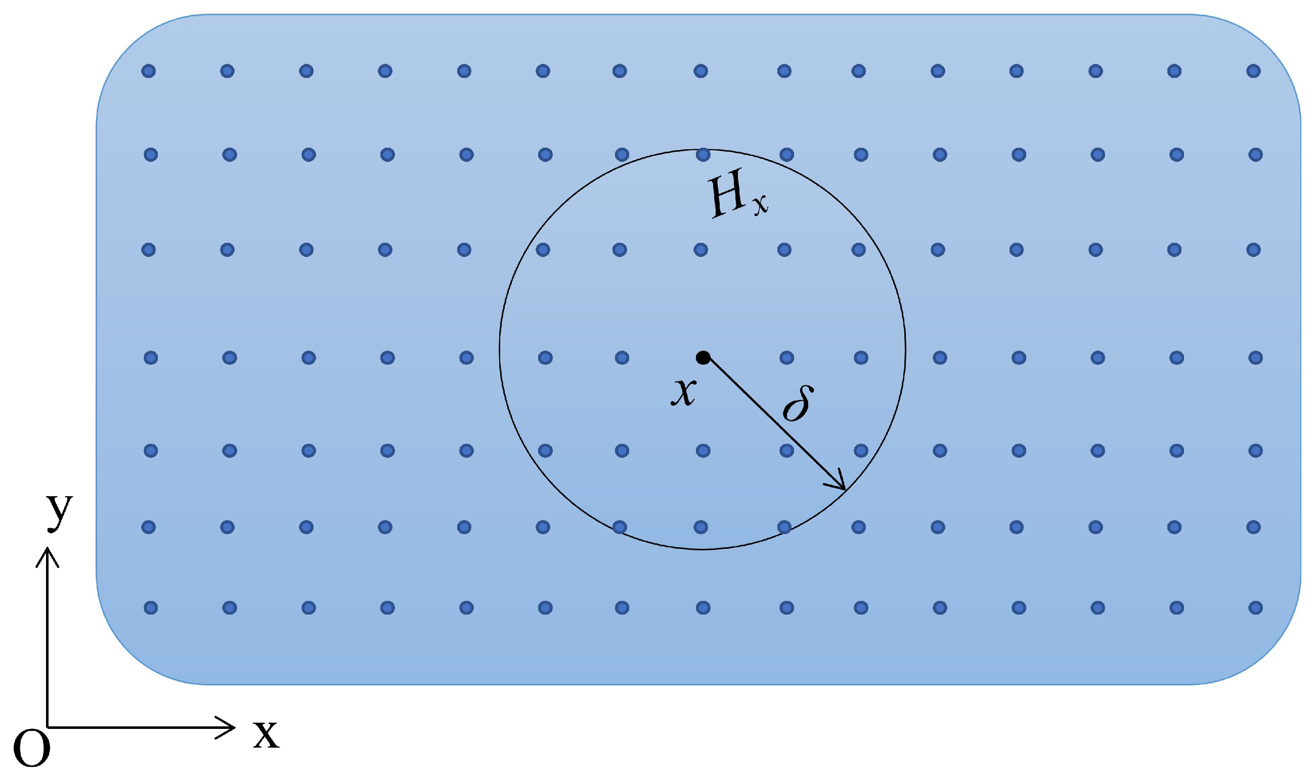
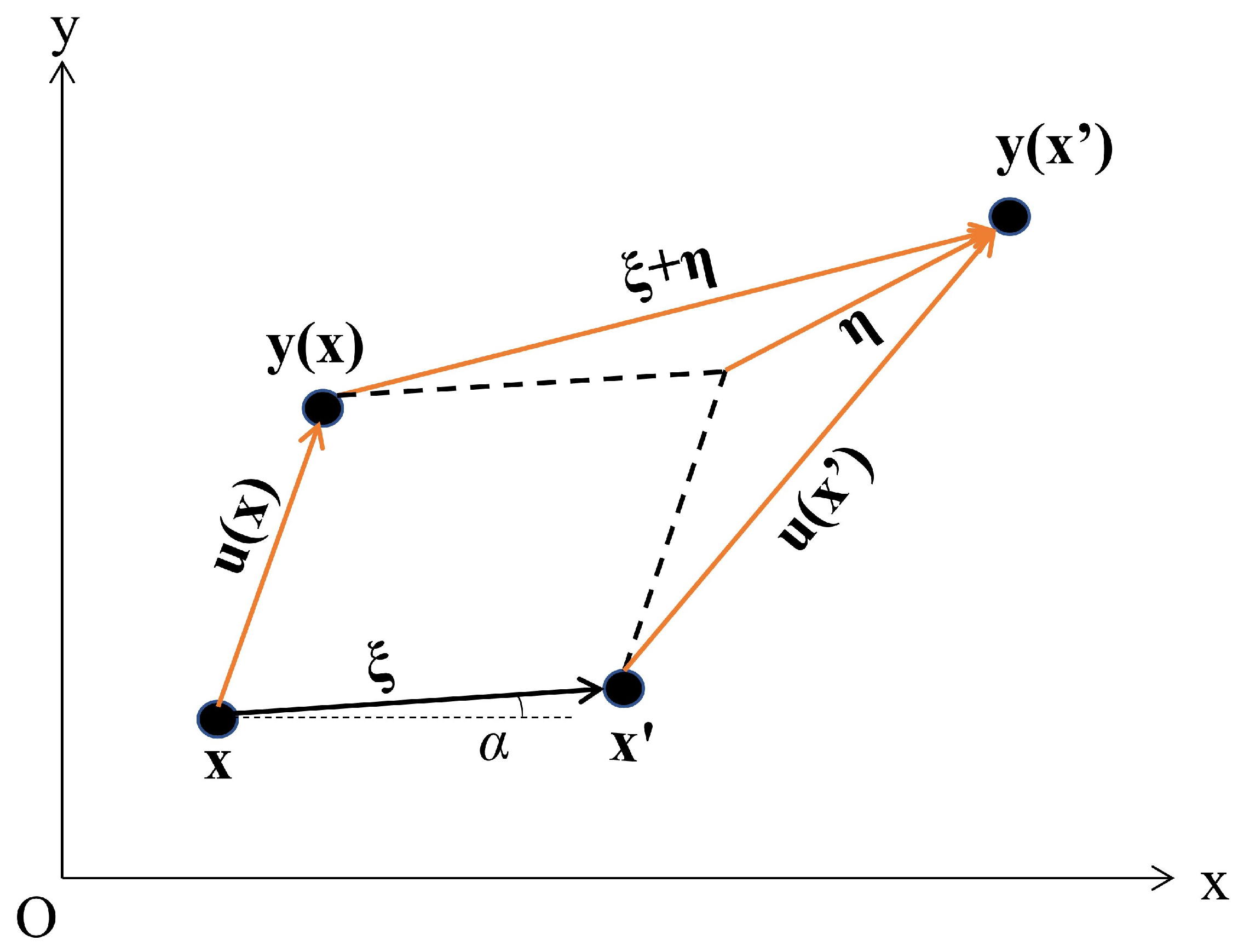
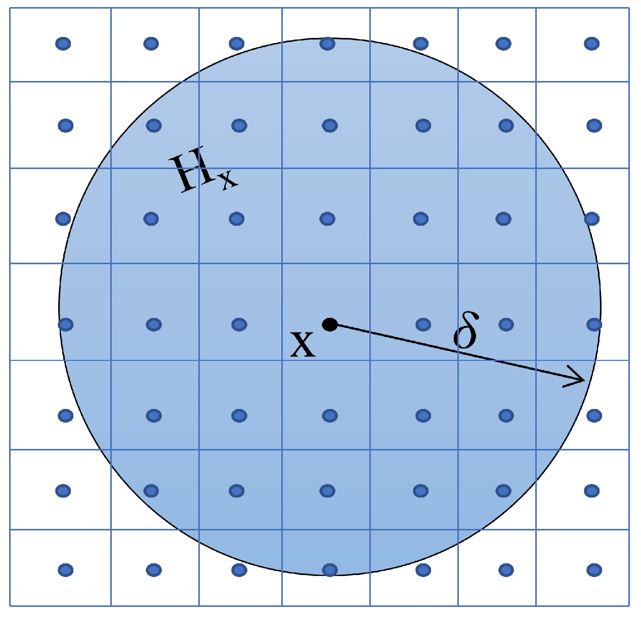
2.1. A Brief Introduction to PD

In PD, each node x interacts with its neighboring nodes within a zone of influence, referred to as the horizon, denoted by $H_x$. The most commonly used horizon is a sphere in a 3D model and a disk with thickness H and radius $\delta$ in a 2D model, as shown in Figure 1. In BBPD, the interaction between two particles connected by a bond is described by [8,26]:

$$\begin{array}{cc}\hfill \rho \ddot{\mathbf{u}}(\mathbf{x},t)d{V}_x& ={\int }_{H_x}\mathbf{f}(\mathbf{u}\left({\mathbf{x}}^{\prime }\right)-\mathbf{u}\left(\mathbf{x}\right),{\mathbf{x}}^{\prime }-\mathbf{x},t)d{V}_{x^{\prime }}d{V}_x\hfill \\ \hfill & +\mathbf{b}(\mathbf{x},t)d{V}_x\hfill \end{array}$$

(1)

where ${\mathbf{x}}^{\prime }-\mathbf{x}$ is the relative position between the particles before deformation, $\mathbf{u}\left({\mathbf{x}}^{\prime }\right)-\mathbf{u}\left(\mathbf{x}\right)$ is the relative displacement of the particles after deformation, $\rho$ is the density of the node, $\mathbf{f}(\mathbf{u}\left({\mathbf{x}}^{\prime }\right)-\mathbf{u}\left(\mathbf{x}\right),{\mathbf{x}}^{\prime }-\mathbf{x},t)$ is the bond force density, and $\mathbf{b}(\mathbf{x},t)$ is the external force per unit volume acting on the element x. $V_x$ and $V_{x^{\prime }}$ are the volumes of the interacting nodes x and $x^{\prime }$, respectively. $H_x$ is the horizon of node x, which defines the range of interaction between node x and other nodes in the system. The body force density can be expressed in terms of the relative positions of the nodes before and after deformation as follows:

$$\mathbf{f}(\mathbf{u}\left({\mathbf{x}}^{\prime }\right)-\mathbf{u}\left(\mathbf{x}\right),{\mathbf{x}}^{\prime }-\mathbf{x},t)=\left\{\begin{array}{cc}Ce\mathbf{K}\hfill & \mathrm{if}{x}^{\prime }\in H_x\hfill \\ 0\hfill & \mathrm{if}{x}^{\prime }\notin H_x\hfill \end{array}\right.$$

(2)

where C is a micromodulus function related to the elastic properties of the material, $e=|\mathbf{y}\left({\mathbf{x}}^{\prime }\right)-\mathbf{y}\left(\mathbf{x}\right)|-|{\mathbf{x}}^{\prime }-\mathbf{x}|$ is defined as the bond deformation of the interacting nodes. The term $\mathbf{y}\left({\mathbf{x}}^{\prime }\right)-\mathbf{y}\left(\mathbf{x}\right)$ represents the relative position of particles after displacement, and $\mathbf{K}$ is the unit vector of the nodes after deformation given by $\mathbf{K}={\displaystyle \frac{\mathbf{y}\left({\mathbf{x}}^{\prime }\right)-\mathbf{y}\left(\mathbf{x}\right)}{|\mathbf{y}\left({\mathbf{x}}^{\prime }\right)-\mathbf{y}\left(\mathbf{x}\right)|}}$. In classical deformation-based BBPD, the bond force is determined by a single micromodulus function, denoted as C. This micromodulus function is derived by matching the strain energy in classical continuum mechanics with the strain energy of a node in PD. However, this approach of using a single micromodulus parameter restricts the Poisson’s ratio to a value of 1/4 for 3D and plane-strain conditions, and 1/3 for plane-stress conditions.

If we denote the relative displacement vector between the particles connected by a bond as $\mathit{\eta }=\mathbf{u}\left({\mathbf{x}}^{\prime }\right)-\mathbf{u}\left(\mathbf{x}\right)$, and the initial position vector between the particles as $\mathit{\xi }$, then the relative position vector between the particles after displacement is given by $\mathit{\xi }+\mathit{\eta }$. The interaction between two particles in PD is illustrated in Figure 2. The energy density associated with each bond in the traditional BBPD model is given by the following:

$$w={\displaystyle \frac{1}{2}}C{e}^2$$

(3)

and the force density is expressed as follows:

$${\displaystyle \frac{\delta w}{\delta \eta }}=\mathbf{f}(\mathit{\eta },\mathit{\xi },t)=Ce\mathbf{K}$$

(4)

where $e=|\mathit{\xi }+\mathit{\eta }|-\left|\mathit{\xi }\right|$ and K = ${\displaystyle \frac{\mathit{\xi }+\mathit{\eta }}{\left|\mathit{\xi }+\mathit{\eta }\right|}}$

2.2. Virtual Internal Bond Method

Peridynamics employs an approach where the continuous solid is discretized into numerous distinct nodes distributed across the defined domain, each occupying specific positions and volumes. This discretization facilitates the use of an energy equation derived from the virtual internal bond (VIB) method [33]. In the VIB method, the derivations of elongation and rotational energies of the bonds are independent of the strain term, making the method well-suited for deformation-based PD.

In the virtual internal bond (VIB) model, the solid is conceptualized as comprising an extensive array of discrete mass particles at the microscopic scale, emphasizing a granular representation of the material’s structure and behavior within the framework of the model. Initially developed by considering the radial displacement of the virtual bonds and used successfully for the study of cracks [33], it was later expanded to consider the rotation of the virtual bonds [34,35], which eliminated the restriction of Poisson’s ratio suffered by the older approach. The particles in modified VIB are allowed to both elongate radially and rotate along an axis, as shown in Figure 3. The energy potential of a bond in modified VIB is given by the following:

$$U={\displaystyle \frac{1}{2}}{C}_l{l}^2+{\displaystyle \frac{1}{2}}{C}_r{\theta }_1^2+{\displaystyle \frac{1}{2}}{C}_r{\theta }_2^2+{\displaystyle \frac{1}{2}}{C}_r{\theta }_3^2$$

(5)

where $C_l$ is the elongation stiffness, $C_r$ is the rotational stiffness of the bonds, l is the radial elongation of the bond, and ${\theta }_1$, ${\theta }_2$, and ${\theta }_3$ are the rotation angles of the bonds along the x, y, and z axes, respectively. However, in this study, we shall focus on 2D models (Figure 3b) only.

We can reformulate the above equation to consider the tangential displacement for small angular rotations along the axes. If ${\gamma }_1$ represents the tangential displacement along the x-axis and ${\gamma }_2$ represents the tangential displacement along the y-axis corresponding to ${\theta }_1$ and ${\theta }_2$, respectively, we can write the following:

$${\gamma }_1={\theta }_1\ast \xi ,{\gamma }_2={\theta }_2\ast \xi$$

(6)

In Equation (6), $\xi$ is the length of the bond. We can modify the energy equation of the bonds to incorporate the tangential displacement and tangential stiffness as follows:

$$U={\displaystyle \frac{1}{2}}{C}_l{l}^2+{\displaystyle \frac{1}{2}}{C}_t{\gamma }_1^2+{\displaystyle \frac{1}{2}}{C}_t{\gamma }_2^2$$

(7)

We replace $C_r$ with $C_t$ to account for the tangential displacement stiffness ($C_r$ is the rotational stiffness). The elongation of a normal bond is written as follows:

$$l=\xi {\lambda }_i{ϵ}_{ij}{\lambda }_j$$

(8)

The angle of rotation of a bond along the coordinate axes is written as follows:

$$\begin{array}{c}\hfill \left\{\begin{array}{cc}\hfill {\theta }_1& ={\lambda }_i{ϵ}_{ij}{\omega }_j^{\prime },\hfill \\ \hfill {\theta }_2& ={\lambda }_i{ϵ}_{ij}{\omega }_j^{″}.\hfill \end{array}\right.\end{array}$$

(9)

Thus, Equation (6) can be modified as follows:

$$\begin{array}{c}\hfill \left\{\begin{array}{c}\hfill {\gamma }_1=\xi {\lambda }_i{ϵ}_{ij}{\omega }_j^{\prime },\\ \hfill {\gamma }_2=\xi {\lambda }_i{ϵ}_{ij}{\omega }_j^{\prime \prime }\end{array}\right.\end{array}$$

(10)

In Equations (8) and (9), $\lambda =\{cos\alpha ,sin\alpha \}$ denotes the orientation of the bond connecting two nodes, and $\omega$ is a unit vector perpendicular to $\lambda$. The corresponding values are given by ${\omega }^{\prime }=\{{sin}^2\alpha ,-sin\alpha cos\alpha \}$ and ${\omega }^{″}=\{-sin\alpha cos\alpha ,{cos}^2\alpha \}$. For the computation of $\omega$, readers are referred to Zhang and Ge [34]. Here, $\alpha$ represents the angle made by the bond with the x-axis (Figure 2), and ${ϵ}_{ij}$ denotes the strain tensor. Substituting Equations (8) and (10) into Equation (7), the strain energy of a bond in the modified VIB method can be obtained.

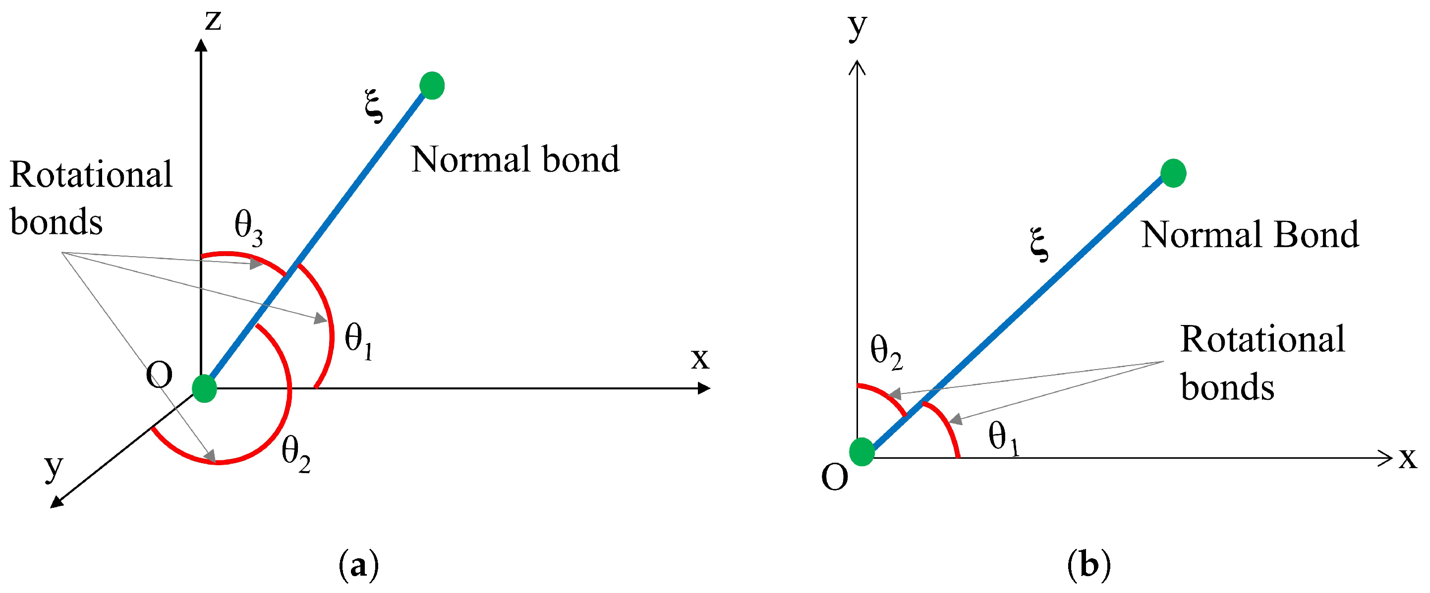
2.3. Two Parameter PD

The pairwise interaction between nodes in the traditional approach only considers the effect of bond strain in the radial direction. In the modified deformation-based BBPD method, the tangential displacement component is also included when considering the interaction of nodes. Thus, interacting nodes exhibit stiffness in both the normal and tangential directions, similar to bonds in VIB, as shown in Figure 4. If we denote the normal stiffness by $C_l$ and the tangential stiffness by $C_t$, we can modify Equations (3) and (4) to account for the contributions of both normal and tangential displacements as follows:

$$\begin{array}{c}\hfill w={\displaystyle \frac{1}{2}}{C}_l{\eta }_l^2+{\displaystyle \frac{1}{2}}{C}_t{\eta }_t^2\end{array}$$

(11)

$$\begin{array}{c}\hfill \mathbf{f}(\mathit{\eta },\mathit{\xi },t)=C_l{\eta }_l\overrightarrow{e_l}+C_t{\eta }_t\overrightarrow{e_t}\end{array}$$

(12)

where ${\eta }_l$ and ${\eta }_t$ denote the projections of the relative displacement vector ($\mathit{\eta }$) in the normal and tangential directions of the original bond vector, and $\overrightarrow{e_l}$ and $\overrightarrow{e_t}$ denote the unit vectors in the normal and tangential directions, respectively. The unit vectors $\overrightarrow{e_l}={\displaystyle \frac{\mathit{\xi }}{\left|\mathit{\xi }\right|}}$ and $\overrightarrow{e_t}$ are oriented such that $\overrightarrow{e_t}·\overrightarrow{e_l}=0$.

If $U_p$ denotes the energy density of a PD bond, we can write the total strain energy density for a PD particle as follows:

$$U_{peri}={\displaystyle \frac{1}{2}}{\int }_{H_x}{U}_{p}d{V}_{x^{\prime }}$$

(13)

For a 2D domain with thickness H, using Equation (7) as the energy density of PD nodes ($U_p=U$), the strain energy density can be expanded as follows:

$$\begin{array}{cc}\hfill U_{peri}& ={\displaystyle \frac{H}{2}}{\int }_0^{2\pi }{\int }_0^{\delta }U\xi d\xi d\alpha \hfill \\ \hfill & =H{\delta }^4\left({\displaystyle \frac{3\pi C_l{ϵ}_{11}^2}{64}}+{\displaystyle \frac{\pi C_l{ϵ}_{11}{ϵ}_{22}}{32}}+{\displaystyle \frac{\pi C_l{ϵ}_{12}^2}{16}}+{\displaystyle \frac{3\pi C_l{ϵ}_{22}^2}{64}}+{\displaystyle \frac{\pi C_t{ϵ}_{11}^2}{64}}-{\displaystyle \frac{\pi C_t{ϵ}_{11}{ϵ}_{22}}{32}}\right.\hfill \\ \hfill & +\left.{\displaystyle \frac{\pi C_t{ϵ}_{12}^2}{16}}+{\displaystyle \frac{\pi C_t{ϵ}_{22}^2}{64}}\right)\hfill \end{array}$$

(14)

The strain energy density obtained from classical continuum mechanics is written for the plane-stress condition and the plane-strain condition as [36]:

$$\begin{array}{c}\hfill \begin{array}{cc}\hfill U_{ccm}^{stress}=& {\displaystyle \frac{E}{2(1-{\mu }^2)}}({ϵ}_{11}^2+{ϵ}_{22}^2)+{\displaystyle \frac{E\mu }{1-{\mu }^2}}{ϵ}_{11}{ϵ}_{22}+{\displaystyle \frac{E(1-\mu )}{2(1-{\mu }^2)}}{ϵ}_{12}^2\hfill \end{array}\end{array}$$

(15)

$$\begin{array}{c}\hfill \begin{array}{cc}\hfill U_{ccm}^{strain}=& {\displaystyle \frac{E(1-\mu )}{2(1+\mu )(1-2\mu )}}({ϵ}_{11}^2+{ϵ}_{22}^2)+{\displaystyle \frac{E\mu }{(1+\mu )(1-2\mu )}}{ϵ}_{11}{ϵ}_{22}+{\displaystyle \frac{E}{2(1+\mu )}}{ϵ}_{12}^2\hfill \end{array}\end{array}$$

(16)

Equating the coefficients of ${ϵ}_{11}^2$, ${ϵ}_{22}^2$, and ${ϵ}_{11}{ϵ}_{22}$ from Equations (14)–(16), we can obtain the values of $C_l$ and $C_t$ for plane-stress and plane-strain conditions, respectively. For the plane-stress condition, we have the following:

$$\begin{array}{c}\hfill \left\{\begin{array}{cc}\hfill C_l& ={\displaystyle \frac{8E(1+\mu )}{\pi (1-{\mu }^2){\delta }^{4}H}},\hfill \\ \hfill C_t& ={\displaystyle \frac{8E(1-3\mu )}{\pi (1-{\mu }^2){\delta }^{4}H}}.\hfill \end{array}\right.\end{array}$$

(17)

For the plane-strain condition, we have the following:

$$\begin{array}{c}\hfill \left\{\begin{array}{cc}\hfill C_l& ={\displaystyle \frac{8E}{\pi (1+\mu )(1-2\mu ){\delta }^{4}H}},\hfill \\ \hfill C_t& ={\displaystyle \frac{8E(1-4\mu )}{\pi (1+\mu )(1-2\mu ){\delta }^{4}H}}.\hfill \end{array}\right.\end{array}$$

(18)

It is important to note that the stiffness coefficients are consistent and invariant regardless of the specific combinations of strains being equated. From Equations (17) and (18), it is evident that the limiting value of Poisson’s ratio in the plane-stress condition is ≤1/3, and it is ≤1/4 in the plane-strain condition.

Failure Criteria

In strain-based BBPD, the failure criteria are typically defined in terms of critical normal and tangential strains, enabling the modeling of bond failure under tension, compression, and shear. However, the peridynamic equations employed in our study use bond deformation instead of bond strain. Therefore, it is crucial to establish failure criteria based on bond deformation. Under 2D conditions, the fracture energy of a material (G) can be related to the critical energy density ($u_c$) as follows [37]:

$$G=2{\int }_0^{\delta }{\int }_z^{\delta }{\int }_0^{co{s}^{-1}\left({\displaystyle \frac{z}{\xi }}\right)}{u}_c\xi d\theta d\xi$$

(19)

To include the failure of bonds due to the bond strains in the normal direction and tangential direction, Feng and Zhou [20] defined the critical bond strain in the normal direction utilizing mode-I critical fracture energy and the critical bond strain in the tangential direction utilizing mode-II fracture energy, which are written as follows:

$$\begin{array}{cc}\hfill G_I(1-C_{s1})& =2{\int }_0^{\delta }{\int }_z^{\delta }{\int }_0^{{cos}^{-1}\left({\displaystyle \frac{z}{\xi }}\right)}{u}_I\xi d\theta d\xi dz\hfill \\ \hfill \Rightarrow G_I(1-C_{s1})& =2{\int }_0^{\delta }{\int }_z^{\delta }{\int }_0^{{cos}^{-1}\left({\displaystyle \frac{z}{\xi }}\right)}{\displaystyle \frac{1}{2}}{\eta }_{ltc}^2{C}_l\xi d\theta d\xi dz\hfill \end{array}$$

(20)

$$\begin{array}{cc}\hfill G_{II}\left(C_{s2}\right)& =2{\int }_0^{\delta }{\int }_z^{\delta }{\int }_0^{{cos}^{-1}\left({\displaystyle \frac{z}{\xi }}\right)}{u}_{II}\xi d\theta d\xi dz\hfill \\ \hfill \Rightarrow G_{II}\left(C_{s2}\right)& =2{\int }_0^{\delta }{\int }_z^{\delta }{\int }_0^{{cos}^{-1}\left({\displaystyle \frac{z}{\xi }}\right)}{\displaystyle \frac{1}{2}}{\eta }_{ttc}^2{C}_t\xi d\theta d\xi dz\hfill \end{array}$$

(21)

where $C_{s1}$ is the ratio of bond shear energy to total strain energy in the case of tensile deformation of bonds, $C_{s2}$ is the ratio of bond shear energy to total strain energy in the case of shear deformation of the bonds, $u_I$ is the bond energy density considering only tensile deformation, and $u_{II}$ is the bond energy density considering only tangential deformation.

When the bond undergoes only tensile deformation and shear deformation, the elongations and the rotation of the bonds are given by Equations (8) and (9), respectively, and are written as follows:

$$\begin{array}{c}\hfill \left\{\begin{array}{cc}\hfill l& ={ϵ}_t\xi {cos}^2\alpha ,\hfill \\ \hfill {\gamma }_1& ={ϵ}_t\xi {sin}^2\alpha cos\alpha ,\hfill \\ \hfill {\gamma }_2& =-{ϵ}_t\xi sin\alpha {cos}^2\alpha \hfill \end{array}\right.\end{array}$$

(22)

$$\begin{array}{c}\hfill \left\{\begin{array}{cc}\hfill l& ={ϵ}_s\xi sin\alpha cos\alpha ,\hfill \\ \hfill {\gamma }_1& ={ϵ}_s\xi {sin}^3\alpha ,\hfill \\ \hfill {\gamma }_2& =-{ϵ}_s\xi sin\alpha {cos}^2\alpha \hfill \end{array}\right.\end{array}$$

(23)

In Equations (22) and (23), ${ϵ}_t$, and ${ϵ}_s$ represent the tensile and shear strain, respectively, and $\alpha$ denotes the angle made by the bond with the x-axis.

The total energy of a PD particle under tensile deformation is given by substituting Equation (22) in Equation (13), which is written as follows:

$$\begin{array}{c}\hfill U_{T1}={\displaystyle \frac{\pi {\delta }^4{ϵ}_t^2}{64}}\left(3C_l+C_t\right)\end{array}$$

(24)

The shear energy of the particle is given by the following:

$$\begin{array}{c}\hfill U_{s1}={\displaystyle \frac{\pi {\delta }^4{ϵ}_t^2}{64}}·C_t\end{array}$$

(25)

We obtain $C_{s1}$ from Equations (24) and (25) for the plane-stress condition as follows:

$$\begin{array}{cc}\hfill C_{s1}& ={\displaystyle \frac{1}{(3\ast C_l/C_t)+1}}\hfill \\ \hfill \Rightarrow C_{s1}& ={\displaystyle \frac{1-3\mu }{4}}\hfill \end{array}$$

(26)

Similarly, the total energy of a PD particle under shear deformation can be obtained from Equations (13) and (23):

$$\begin{array}{c}\hfill U_{T2}={\displaystyle \frac{\pi {\delta }^4{ϵ}_t^2}{64}}\left(C_l+3C_t\right)\end{array}$$

(27)

The shear energy of the particle is given by the following:

$$\begin{array}{c}\hfill U_{s1}={\displaystyle \frac{3\pi {\delta }^4{ϵ}_t^2}{64}}·C_t\end{array}$$

(28)

We obtain $C_{s2}$ from Equations (27) and (28) for the plane-stress condition as follows:

$$\begin{array}{cc}\hfill C_{s2}& ={\displaystyle \frac{1}{(C_l/3\ast C_t)+1}}\hfill \\ \hfill \Rightarrow C_{s2}& ={\displaystyle \frac{3(1-3\mu )}{4(1-2\mu )}}\hfill \end{array}$$

(29)

For Equation (20), the value of $z/\xi \le 1$ and $z/\delta \le 1$. Thus, the equation can be written as follows:

$$\begin{array}{cc}\hfill G_I(1-C_{s1})& =C_l{\eta }_{ltc}^2{\int }_0^{\delta }{\int }_z^{\delta }\xi {cos}^{-1}\left({\displaystyle \frac{z}{\xi }}\right)d\xi dz\hfill \\ \hfill \Rightarrow G_I(1-C_{s1})& =C_l{\eta }_{ltc}^2{\int }_0^{\delta }{\displaystyle \frac{{\delta }^2{cos}^{-1}\left(\frac{z}{\delta }\right)}{2}}-{\displaystyle \frac{z\sqrt{{\delta }^2-z^2}}{2}}dz\hfill \\ \hfill \Rightarrow G_I(1-C_{s1})& ={\displaystyle \frac{C_l{\delta }^3{\eta }_{ltc}^2}{3}}\hfill \end{array}$$

(30)

Similarly, Equation (21) can be written for the case of shear deformation as follows:

$$\begin{array}{cc}\hfill G_{II}\left(C_{s2}\right)& ={\displaystyle \frac{C_t{\delta }^3{\eta }_{ttc}^2}{3}}\hfill \end{array}$$

(31)

Thus, the critical values for tensile deformation (${\eta }_{ltc}$) and tangential displacement (${\eta }_{ttc}$) in Equations (30) and (31) can be expressed with the help of Equations (26) and (29), respectively, as follows:

$$\begin{array}{c}\hfill {\eta }_{ltc}=\sqrt{{\displaystyle \frac{9G_I(1+\mu )}{4{\delta }^{3}H{C}_l}}},{\eta }_{ttc}=\sqrt{{\displaystyle \frac{9G_{II}(1-3\mu )}{4{\delta }^{3}H{C}_t(1-2\mu )}}}\end{array}$$

(32)

Similarly, by employing Mohr–Coulomb criteria to account for the critical deformation in compression, the critical compressive deformation is written as follows:

$$\begin{array}{c}\hfill {\eta }_{lcc}={\displaystyle \frac{(1+sin\beta )}{(1-sin\beta )}}{\eta }_{ltc}\end{array}$$

(33)

where $\beta$ is the friction angle of the material.

To define bond failure in tension, compression, and shear, a history-based scalar function $\varphi$ is introduced, and failure is defined as follows:

$$\begin{array}{cc}\hfill {\varphi }_l& =\left\{\begin{array}{cc}1\hfill & \hfill \mathrm{if}{\eta }_{lcc}\le {\eta }_l\le {\eta }_{ltc}\\ 0\hfill & \hfill \mathrm{otherwise}\end{array}\right.\hfill \end{array}$$

(34)

$$\begin{array}{cc}\hfill {\varphi }_t& =\left\{\begin{array}{cc}1\hfill & \hfill \mathrm{if}|{\eta }_t|\le {\eta }_{ttc}\\ 0\hfill & \hfill \mathrm{otherwise}\end{array}\right.\hfill \end{array}$$

(35)

Equation (34) describes failure in the normal direction, while Equation (35) describes failure in the tangential direction for each bond in the domain. The local damage in the normal direction ($D_l$), tangential direction ($D_t$), and the total damage ($D_T$) of a node is written as follows:

$$\begin{array}{c}\hfill D_l={\displaystyle \frac{{\sum }_{i=1}^n{\varphi }_l\ast \mathsf{\Delta }{V}_{x^{\prime }}}{{\sum }_{i=1}^n\mathsf{\Delta }{V}_{x^{\prime }}}}\end{array}$$

(36)

$$\begin{array}{c}\hfill D_t={\displaystyle \frac{{\sum }_{i=1}^n{\varphi }_t\ast \mathsf{\Delta }{V}_{x^{\prime }}}{{\sum }_{i=1}^n\mathsf{\Delta }{V}_{x^{\prime }}}}\end{array}$$

(37)

$$\begin{array}{c}\hfill D_T=(D_l+D_t)/2\end{array}$$

(38)

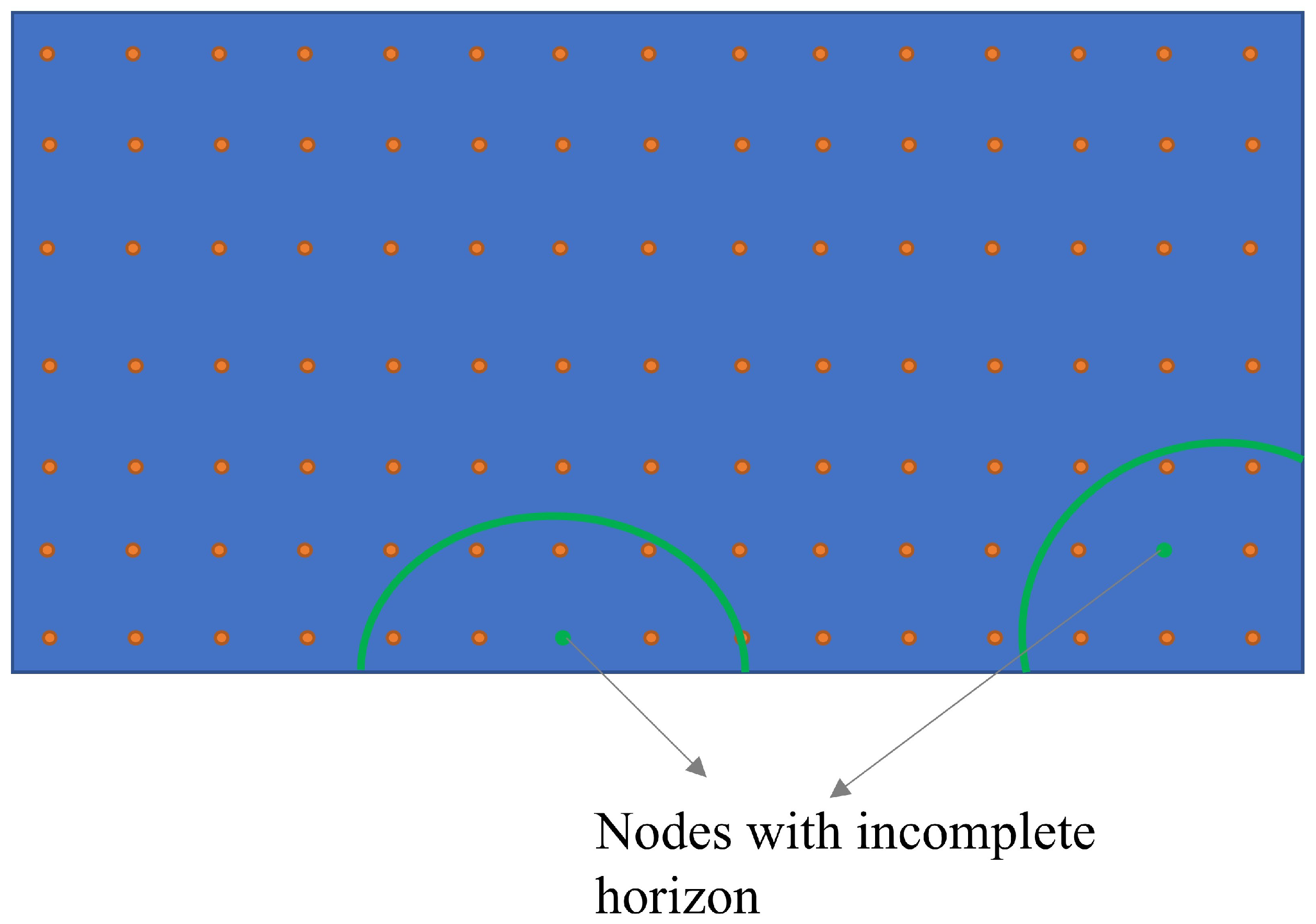
2.4. Stress-Based Correction Factor

In the calculations performed in earlier sections to obtain the strain energy density of a PD particle, a particle within the bulk is considered, where the horizon $\left(H_x\right)$ is properly defined. However, for particles at the edge of the body, as shown in Figure 5, the particles do not have a complete neighborhood. This makes the assumption of a complete horizon invalid, resulting in a softer material response for particles near the free boundary. As a result, numerical errors arise due to incomplete neighborhoods at the boundary or near-boundary nodes. To address this issue, we introduce a novel stress-based correction method in this study.

Since PD is considered an upscaling of molecular dynamics [38], Li et al. [39] showed that the PD stress tensor at a given node can be computed using the virial theorem. This quantity is referred to as the nodal stress throughout this text, which is given as follows:

$$\sigma \left(j\right)={\displaystyle \frac{1}{2V_j}}\sum _{i\ne j}^{N_j}{\xi }_{ij}\otimes F_{ij}$$

(39)

here, $V_j$ is the volume of the node, and ${\xi }_{ij}$ denotes the initial relative position vector, $F_{ij}=f(\eta ,\xi ,t)V_j$.

The correction factor is computed by correcting the stress of a node in a finite domain with a reference from an infinite domain [28]. The correction is based on the assumption that, for a given isotropic solid under elastic conditions, the stress at a particular node in a domain should be the same as the stress experienced by a node in an infinite domain, regardless of the node’s position. To obtain this, uniaxial tension is first applied in the x-direction and then in the y-direction independently. When uniaxial tension is applied in the x-direction with a constant gradient of ${\displaystyle \frac{\delta u}{{\delta }_x}}$, the corresponding displacement field can be written in the following form:

$$\mathbf{u}\left(\mathbf{x}\right)={\left[\begin{array}{cc}{\displaystyle \frac{\delta u}{\delta x}}& -\mu {\displaystyle \frac{\delta u}{\delta x}}\end{array}\right]}^T$$

(40)

From Equation (39), we can obtain the stress in the x direction for node j as follows:

$${\sigma }_{xx}\left(j\right)={\left({\displaystyle \frac{1}{2V_j}}\sum _{i\ne j}^{N_j}{\xi }_{ij}\otimes F_{ij}\right)}_{xx}$$

(41)

If we adopt a similar procedure to apply a constant gradient of ${\displaystyle \frac{\delta v}{\delta y}}$ and obtain the corresponding displacement field, we can write stress in the y-direction as follows:

$${\sigma }_{yy}\left(j\right)={\left({\displaystyle \frac{1}{2V_j}}\sum _{i\ne j}^{N_j}{\xi }_{ij}\otimes F_{ij}\right)}_{yy}$$

(42)

With this, for each node in the domain, we have stress in the x-direction and stress in the y-direction, respectively. This is written as follows:

$$\sigma \left(j\right)=\left[\begin{array}{cc}{\sigma }_{xxj}& {\sigma }_{yyj}\end{array}\right]$$

(43)

In Equation (43), shear stress is neglected because no shear strain is applied within the domain.

In a hypothetical domain with the same material properties as that of the domain under study, depicted in Figure 6, the central node in the figure is surrounded by other points such that the node has a complete horizon. Consequently, this point does not exhibit any directional dependence, allowing for the application of uniaxial tension in only one direction. The stress acting on this node is assumed by dividing the infinite domain into cubic subdomains. The stress acting on this domain is denoted as ${\sigma }_{\infty }$. The effect of the size of the subdomain on the computation of ${\sigma }_{\infty }$ is studied. To elucidate the effect of discretizing the infinite domain on the accuracy of stress computation, subdomains of varying sizes are considered. The material being tested has an elastic modulus of 200 GPa, a density of 7580 ${\mathrm{kg}/\mathrm{m}}^3$, and a strain of 0.001 is applied. It is shown in Figure 7 that the stress of a node in the infinite domain approaches the value given by continuum mechanics when fine discretization is employed. In this study, we apply discretization to ensure that the ideal stress closely matches the analytical value.

Since pairwise interaction is considered in PD, we should obtain the stress correction factor for each bond by considering the contribution of each node in the interacting bonds. If we determine the geometric mean stress for each particle i and j, and write the mean values as follows:

$$\sigma \left(ij\right)=\left[\begin{array}{cc}{\sigma }_{xxij}& {\sigma }_{yyij}\end{array}\right]$$

(44)

We can write the scale factor by considering ellipsoidal variation [28]. For an individual bond, the scale factor is written as follows:

$${\sigma }^{\prime }\left(ij\right)=\left[\begin{array}{cc}{\sigma }_{xxij}^{\prime }& {\sigma }_{yyij}^{\prime }\end{array}\right]$$

(45)

where ${\sigma }_{xxij}^{\prime }={\sigma }_{\infty }/{\sigma }_{xxij}$ and ${\sigma }_{yyij}^{\prime }={\sigma }_{\infty }/{\sigma }_{yyij}$. The bond correction factor for the bond connecting materials i and j is written as follows:

$$k_{ij}={\left({\left({\displaystyle \frac{{\xi }_x}{{\sigma }_{xxij}^{\prime }}}\right)}^2+{\left({\displaystyle \frac{{\xi }_y}{{\sigma }_{yyij}^{\prime }}}\right)}^2\right)}^{-0.5}$$

(46)

where ${\xi }_x$ and ${\xi }_y$ are the x and y components of the initial position vectors of the nodes i and j.

The force density obtained from Equation (12) should be multiplied by the computed factor $k_{ij}$ to obtain the corrected results. The computation of $k_{ij}$ is an iterative process. In this study, computations are repeated 21 times for each bond to obtain the correction factor.

3. Numerical Experiment and Results

In this section, we first present the formulation and implementation of the proposed model using the Cython programming language, followed by the results obtained from the simulations. Where applicable, these results are compared with analytical solutions to assess the accuracy and validity of the model.

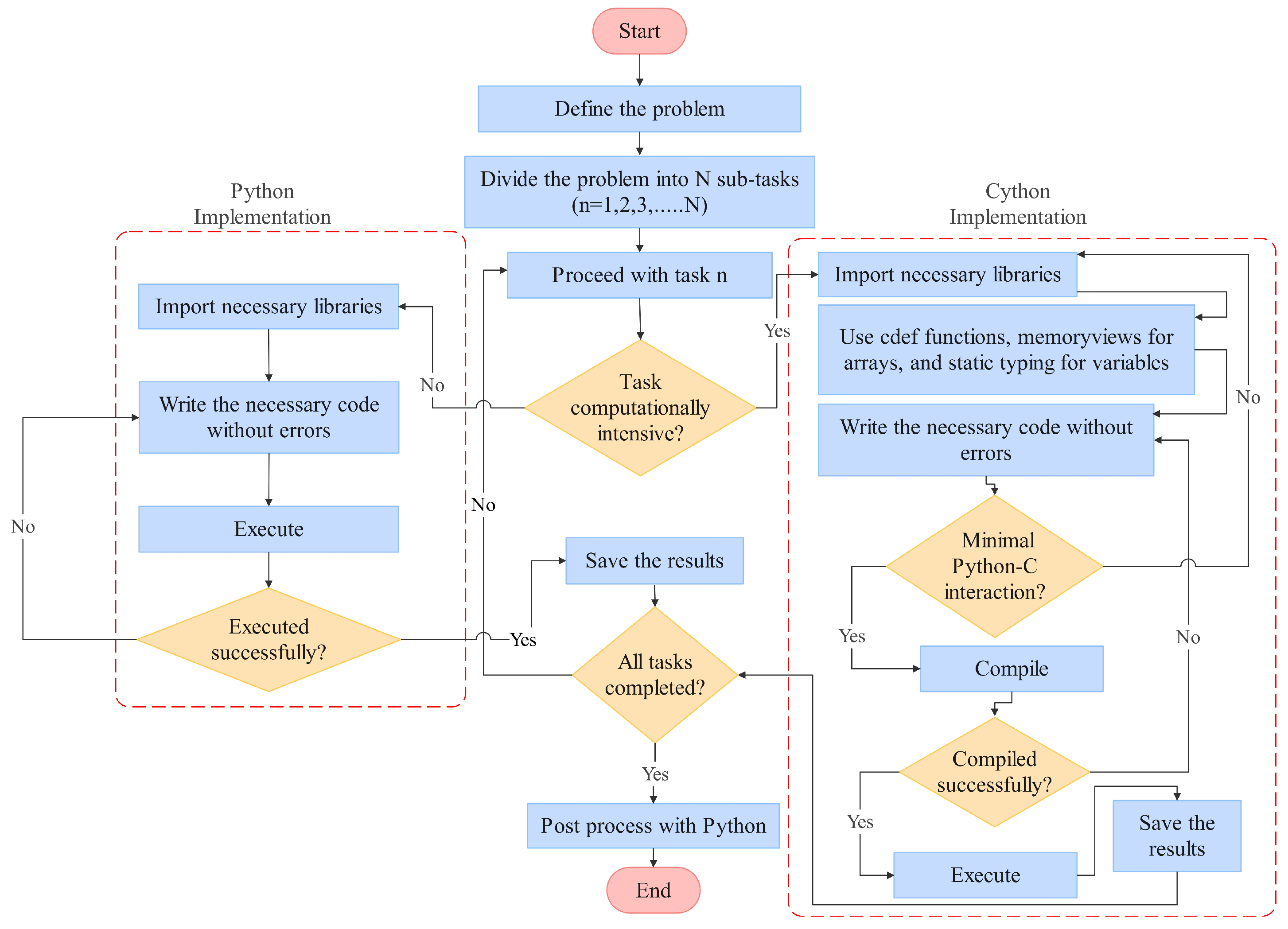
3.1. Implementation of Cython

As a general-purpose language, Python is well known for its clear and concise syntax, making code easier to write, read, and maintain, and the programs written in Python are shorter in length than those written in C/C++ or Java code [40]. It has gained widespread adoption in recent years across various fields such as scientific visualization, data analysis, web development, and machine learning due to its extensive libraries and strong community support. However, in terms of numerical computational performance, this language lags behind popular programming languages used for numerical computations like FORTRAN, C/C++ [41].

Cython allows Python code to achieve near-C-level performance with only minimal modifications. Unlike standard Python, which is executed in real time by the interpreter, Cython code is pre-compiled. This pre-compilation step enables Cython to bypass the overhead of the Python interpreter, allowing performance-critical parts of the code to run at C-like speeds with relatively minor changes to the original Python syntax. This preserves the readability of the code while gaining the decent speed necessary for PD simulations. A flowchart illustrating the implementation of Cython in this study is provided in Figure 8.

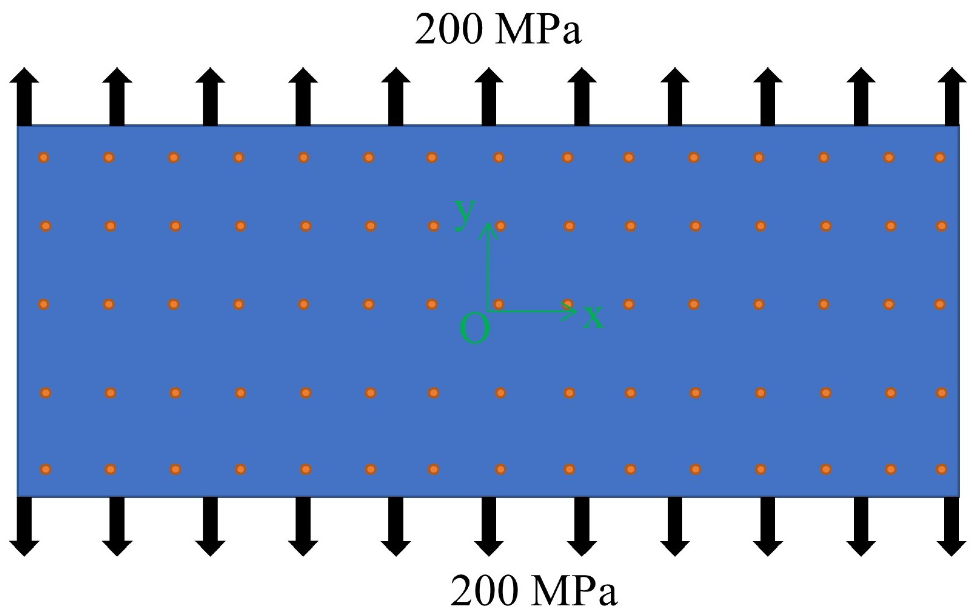
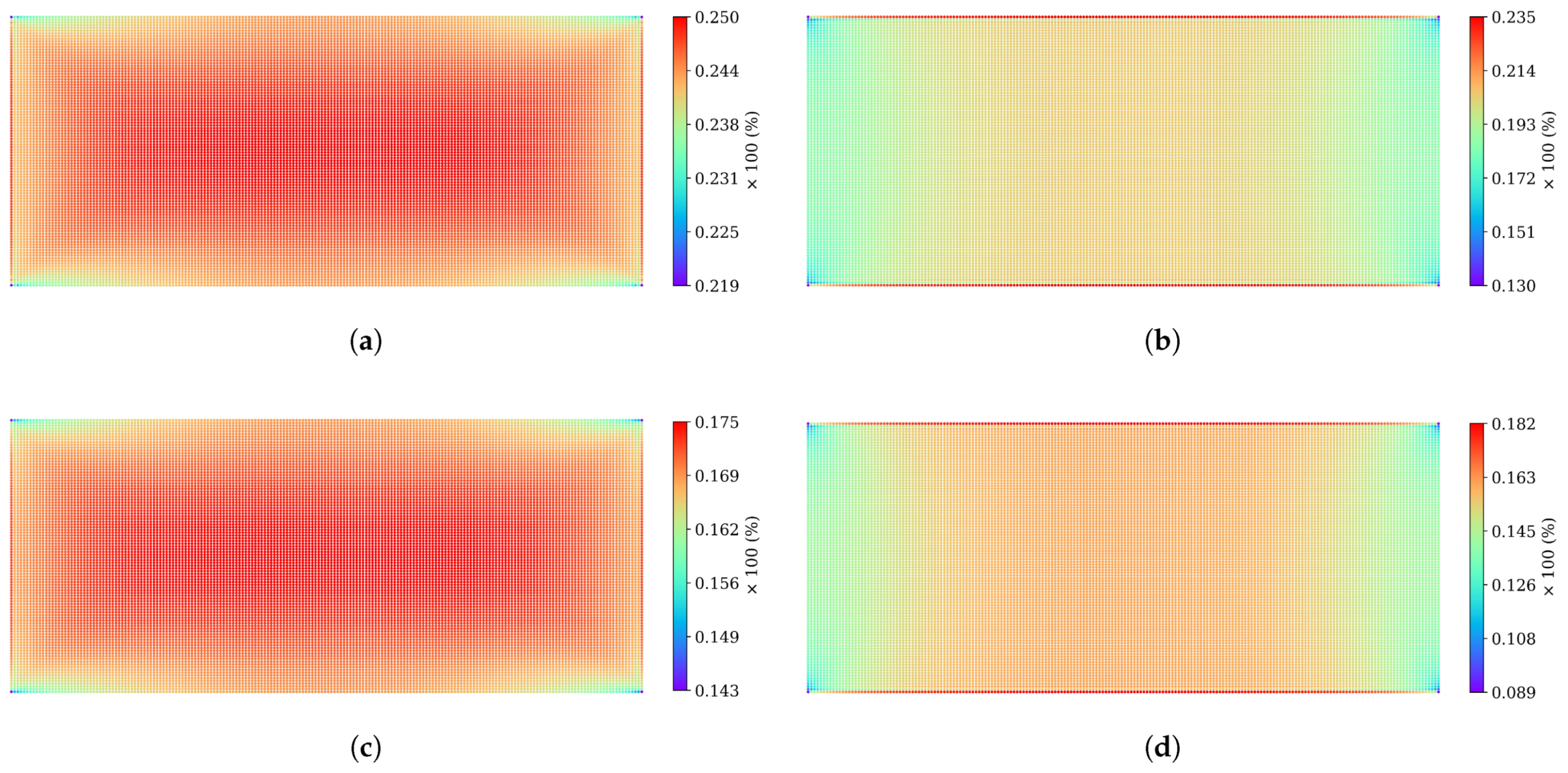
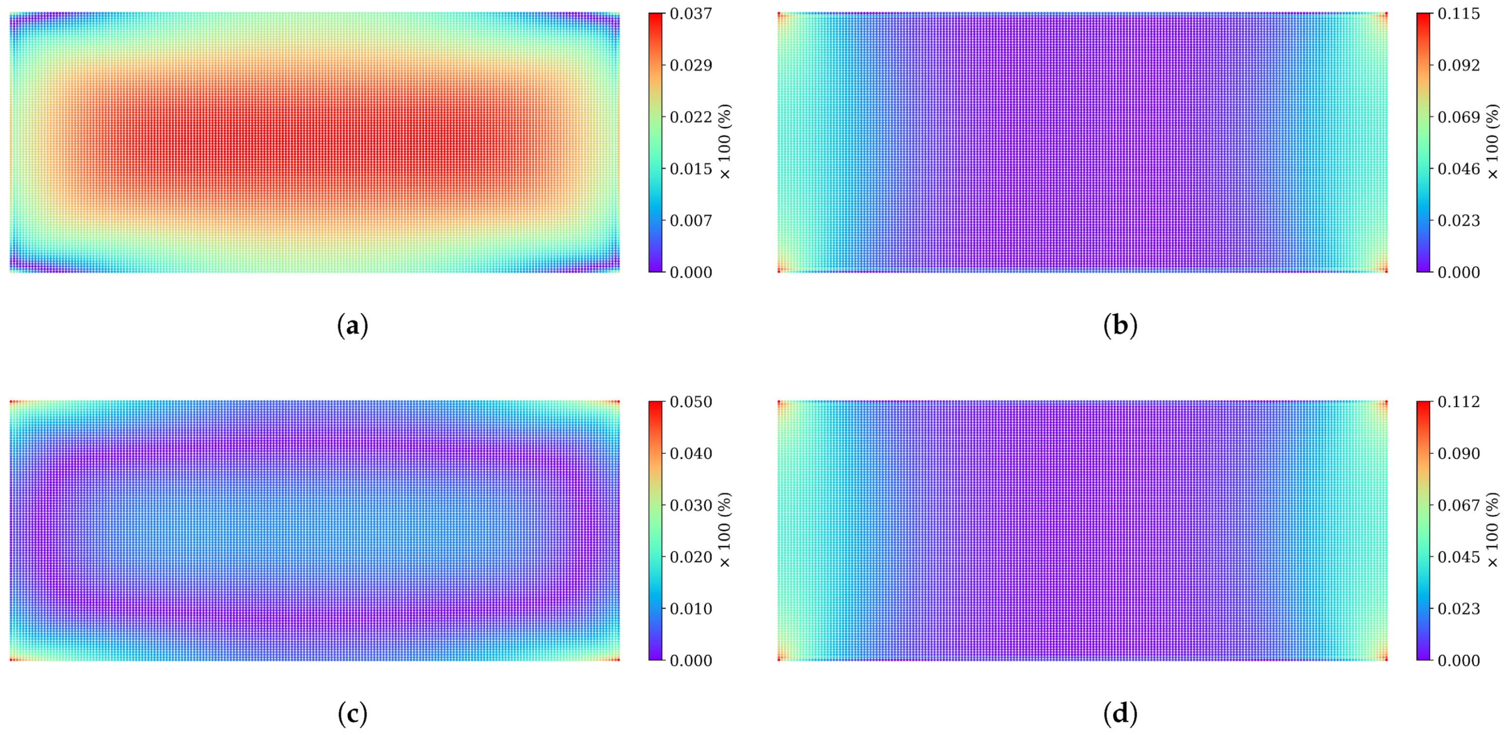
3.2. 2D Plate Under Uniaxial Loading

The simulation was performed on a 2D rectangular plate subjected to uniaxial tensile loading, as depicted in Figure 9, to address the linear elastic problem without bond failure. The proposed model was then used to numerically predict the effective Poisson’s ratio. The plate has dimensions of 0.5 m in height and 1 m in width, a Young’s modulus of 200 GPa, and a variable Poisson’s ratio to illustrate its influence on the effectiveness of the proposed method. A tensile stress of ${\sigma }_{yy}=200\mathrm{MPa}$ is applied to the top and bottom of the rectangular plate. The steady-state solutions are obtained using the adaptive dynamic relaxation technique [42]. In PD, one of the important parameters governing the accuracy of the model and the computational time of the model is the horizon. Several experiments have been conducted to determine the appropriate horizon size of a PD model [13,14,43]. In most cases, a horizon size of 3–5 times the size of a node is preferred. In our study, the rectangular plate was discretized into 20,000 nodes with a node spacing ($\mathsf{\Delta }x$) of 5 mm and a horizon of 3$\mathsf{\Delta }x$. Each simulation was iterated 2000 times to obtain a steady solution.

Loading is applied along the y-axis, and if $\mu$ is the Poisson’s ratio of the material currently being studied, the analytical solution for the nodal displacement of a rectangular plate is given by the following:

$$u_x={ϵ}_{yy}\ast \mu \ast -x,u_y={ϵ}_{yy}\ast y$$

(47)

If we denote the displacement computed from numerical simulations in the x and y directions as $u_x^{\prime }$ and $u_y^{\prime }$, respectively, then the error can be computed as follows:

$$e_x={\displaystyle \frac{|u_x^{\prime }-u_x|}{u_x}},e_y={\displaystyle \frac{|u_y^{\prime }-u_y|}{u_y}}$$

(48)

The analytical displacement values for the rectangular plate are calculated using Equation (47) and compared with the simulation results. Poisson’s ratio and measured maximum displacement errors obtained from the simulations are presented in

Table 1. Comparison of maximum absolute values of errors before and after correction for plane-stress condition.

Poisson’s Ratio	${\mathit{e}}_{\mathit{x}}$ (%)	${\mathit{e}}_{\mathit{y}}$ (%)	Computed Poisson’s Ratio	Remarks
0.0	-	22.074	0.0	Uncorrected
0.0	-	8.482	0.0	Corrected
0.1	23.973	22.674	0.124	Uncorrected
0.1	5.144	7.658	0.104	Corrected
0.2	24.983	23.468	0.249	Uncorrected
0.2	3.680	11.545	0.205	Corrected
0.3	26.611	24.587	0.378	Uncorrected
0.3	7.224	16.532	0.311	Corrected

. To illustrate the distribution of error within the rectangular plate, Figure 10 presents the absolute error values in the x and y displacements for a Poisson’s ratio of 0.1. As shown in the table, the displacement errors in both the x and y directions are notably reduced following the correction procedure. A similar trend is observed for Poisson’s ratio, where the uncorrected PD model overestimates the values. After correction, the estimated Poisson’s ratios were 0, 0.104, 0.205, and 0.311 for the reference values of 0, 0.1, 0.2, and 0.3, respectively. Prior to the correction, the corresponding values were 0, 0.124, 0.249, and 0.378. However, despite significant corrections in the displacement values of PD nodes, higher absolute errors persist at the corners of the rectangle compared to other areas in the domain.

To further illustrate the competency of the proposed method, we compared the accuracy of the proposed method with the existing energy-based correction method and presented the results in Figure 11. The energy density of a node in the energy-based method is given by Equation (11). For the energy-based method, if $w_{xij}$ and $w_{yij}$ represent the geometric mean stress for particles i and j in the x and y directions, and $w_{\infty }$ represents the energy density of the central node in the infinite domain, we can write the scale factor for a bond as follows:

$$w^{\prime }\left(ij\right)=\left[\begin{array}{cc}{w}_{xij}^{\prime }& w_{yij}^{\prime }\end{array}\right]$$

(49)

where $w_{xij}^{\prime }=w_{\infty }/w_{xij}$ and $w_{yij}^{\prime }=w_{\infty }/w_{yij}$. Thus, the correction factor $k_{ij}^{\prime }$ can be obtained:

$$k_{ij}^{\prime }={\left({\left({\displaystyle \frac{{\xi }_x}{w_{xij}^{\prime }}}\right)}^2+{\left({\displaystyle \frac{{\xi }_y}{w_{yij}^{\prime }}}\right)}^2\right)}^{-0.5}$$

(50)

Here, ${\xi }_x$ and ${\xi }_y$ have the same meaning, as provided in Equation (46).

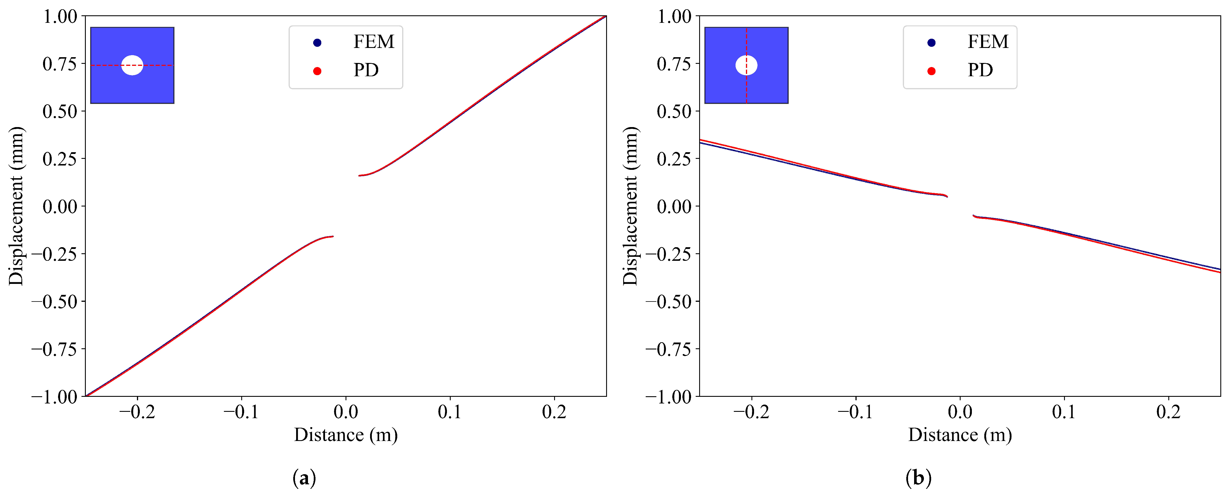
3.3. Rectangular Plate with a Hole

To analyze the accuracy of the model under complex geometry, a rectangular plate with a hole is considered. The dimensions of the plate (Figure 12) are 0.5 m in both length and width, with a hole diameter of 0.025 m. A displacement boundary condition is employed, where the plate is subjected to a tensile displacement of 0.01 m on the left and right edges of the plate. The domain is discretized with material spacing of 0.5 mm ($\mathsf{\Delta }x$) and a horizon of 3 $\mathsf{\Delta }x$. The total number of nodes in the domain is 998,024, and Poisson’s ratio of 1/3 is employed to study how the PD model performs under the limiting case for the plane-stress condition. The accuracy of the proposed PD formulation is assessed through comparison with finite element analysis (FEM) conducted using the open-source software Code_Aster (salome_meca). In the FEM model, the plate is discretized into 4913 nodes and 9332 triangular elements.

The stress distribution near the hole is illustrated in Figure 13. Both the peridynamics (PD) and finite element method (FEM) effectively capture the prominent stress concentration around the hole. The maximum stress near the vicinity of the hole obtained from the PD model was 240 MPa, compared to 252 MPa from the finite element method, indicating good agreement with an error of 4.7% between the two approaches. The displacement of the nodes along the horizontal and the vertical directions along the centerline of the hole is shown in Figure 14. From these figures, it is evident that the PD model performs satisfactorily with good accuracy under complex geometrical conditions.

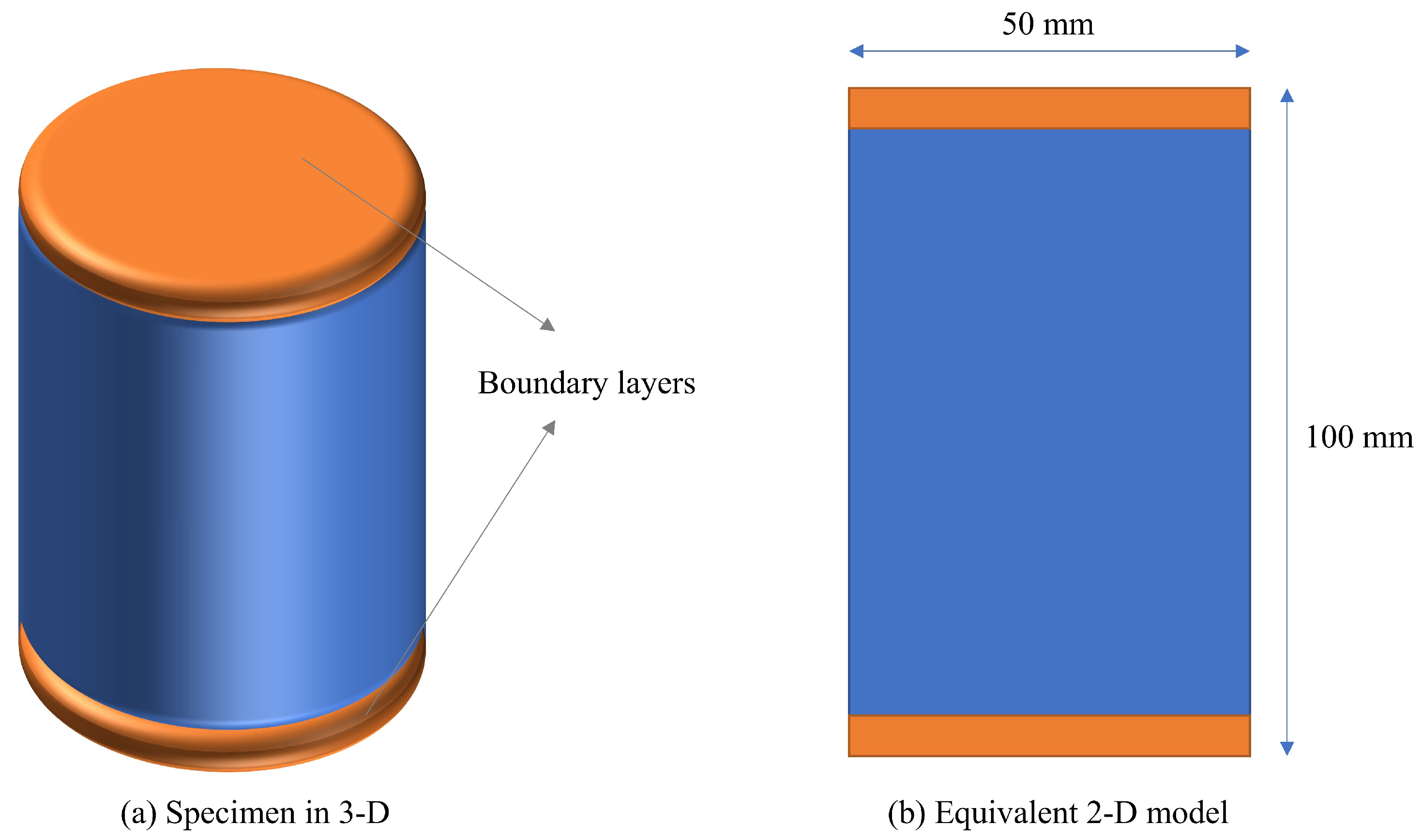
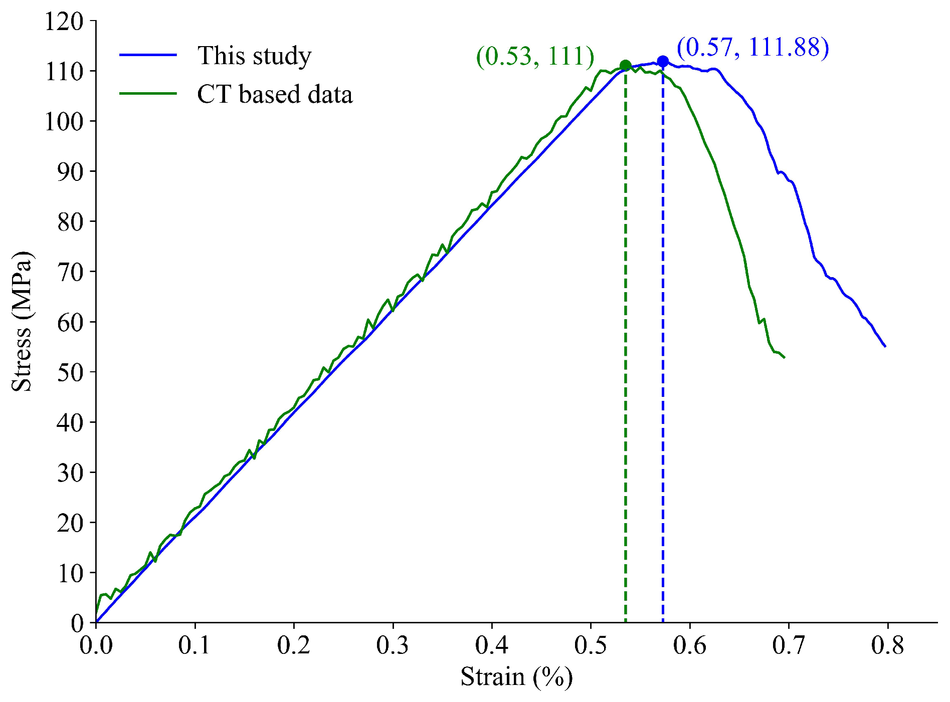
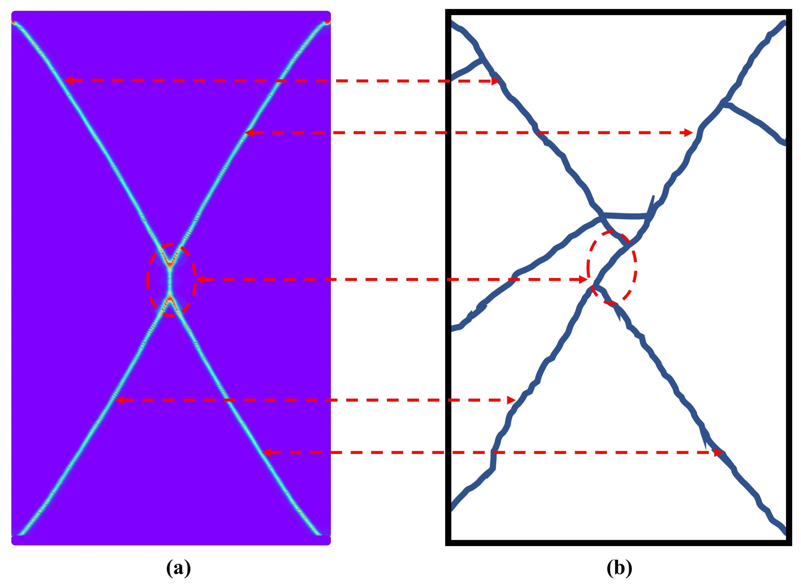
3.4. Uniaxial Compression Test

A uniaxial compressive test is performed and compared with the existing results provided for granite [20]. The material properties of granite are shown in

Table 2. Material properties of granite.

E (GPa)	$\mathit{\rho }$ (kg/m3)	$\mathit{\mu }$	UCS (MPa)	${\mathit{G}}_{\mathit{I}}$ (Jm2)	${\mathit{G}}_{\mathit{II}}$ (Jm2)	$\mathit{\beta }$ (°)
21	2800	0.23	112	93	170	${39}^{\circ }$

. The rectangular specimens have dimensions of 100 mm in height and 50 mm in width. Two boundary layers with a thickness of 3 $\mathsf{\Delta }x$ were formed at the top and bottom of the numerical model, which is shown in Figure 15. The domain is uniformly divided with a material point spacing of $\mathsf{\Delta }x$ = 0.2 mm, and a horizon of 3 $\mathsf{\Delta }x$ is employed. The parameters employed for simulation are shown in

Table 3. Simulation parameters.

Parameters	Values
material spacing	0.0002 m
horizon	0.0006 m
critical tensile deformation $\left({\eta }_{ltc}\right)$	$1.336$ µm
critical compressive deformation $\left({\eta }_{lcc}\right)$	$5.874$ µm
critical tangential deformation $\left({\eta }_{ttc}\right)$	$3.108$ µm
loading rate	${10}^{-7}$ m/s
time step	1 s

.

The stress–strain plot for the simulation is shown in Figure 16. The stress–strain plot obtained in this study closely resembles that obtained in the study by Feng and Zhou [20]. The maximum value of UCS obtained in this study is 111.88 MPa, compared to the experimental value of 112 MPa. Similarly, the value of Young’s modulus of elasticity (E) is 20.67 GPa, compared to the experimental value of 21 GPa. The errors in UCS and E are 0.1% and 1.57%, respectively, when compared to the experimental data. Compared to the CT-based simulation result, the computed UCS in this study is slightly more accurate, as shown in Figure 16. However, the critical strain (the strain corresponding to the peak of the curve) in this study (0.57) is slightly higher than that reported in the experiments (0.53), with an error of 7.5%. It should be noted that, in the 2D study performed by Feng and Zhou [20], the errors in the computation of Young’s modulus and peak strength were reported to deviate from the experimental findings by 4.7% and 3.5%. The model was calibrated from the CT-based data. This suggests that, for the 2D case, deformation-based PD is better suited to characterize Young’s modulus and peak strength of rocks.

The failure process of the specimen is explained with the help of Figure 17. At the time-step of 2000 s, Figure 17a illustrates that tangential bonds at the corners of the specimen fail earlier than the normal bonds. This initial damage at the corners marks the onset of fracture due to the high-stress concentration in these regions. As the simulation progresses, the damage gradually extends from the corners toward the center of the specimen. These damaged zones propagate along diagonal paths moving toward the center of the specimen, forming two intersecting fracture lines. The cracks grow along these diagonals until they meet, producing a characteristic X-shaped failure pattern. This propagation pattern demonstrates how early corner damage controls the overall fracture development under the applied loading. The failure pattern presented in Figure 17b is at a time-step of 3000 s. The X-shaped failure observed here is a common mode under the given test conditions [13,18] and closely matches the failure patterns reported by Feng and Zhou in their CT-based heterogeneous simulations [20]. A comparison between this study and the 2D simulation results from their study is provided in Figure 18. The failure paths in both tests clearly exhibit an X-shaped pattern, with a small bridge forming between the fractures originating from the top and bottom of the specimen, which coalesce at the center.

3.5. Comparison with Existing Method

The current derivation of PD equations (Section 2.3) deviates from the derivation of the original BBPD equations, which are derived considering bond strain. In this study, equations for bond force density and energy density are derived by employing micromodulus and bond deformation. In the prototype micro-elastic (PM) material [8], the term bond constant ‘c’ is used instead of the micromodulus ‘C’. This bond constant is defined as $c=C/\xi$ and is assumed to be proportional to the strain of the bond. The bond force density and bond energy density are computed based on the values of strain rather than using the deformation of the bond. The bond force density for the prototype micro-elastic material is written as follows:

$$\begin{array}{c}\hfill w={\displaystyle \frac{1}{2}}c{s}^2\xi \end{array}$$

(51)

$$\begin{array}{c}\hfill \mathbf{f}(\mathit{\eta },\mathit{\xi },t)=cs\overrightarrow{e}\end{array}$$

(52)

where $s={\displaystyle \frac{|\mathit{\xi }+\mathit{\eta }|-\left|\mathit{\xi }\right|}{\mathit{\xi }}}$ and $\overrightarrow{e}={\displaystyle \frac{\mathit{\xi }+\mathit{\eta }}{|\mathit{\xi }+\mathit{\eta }|}}$

However, this model also suffers from the limitation of a constant value of Poisson’s ratio in both 3D and 2D problems. This has been modified by incorporating the strain of bonds both in normal and tangential directions [12,44]. For plane-stress conditions, the bond constants for normal and tangential directions are written as follows [12]:

$$\begin{array}{c}\hfill c_l={\displaystyle \frac{6E(1+\mu )}{\pi (1-{\mu }^2){\delta }^{3}H}}\\ \hfill c_t={\displaystyle \frac{6E(1-3\mu )}{\pi (1-{\mu }^2){\delta }^{3}H}}\end{array}$$

(53)

The bond strain density and bond force density are obtained as follows:

$$\begin{array}{c}\hfill w={\displaystyle \frac{1}{2}}{c}_l{\left({\displaystyle \frac{{\eta }_l}{\xi }}\right)}^2\xi +{\displaystyle \frac{1}{2}}{c}_t{\left({\displaystyle \frac{{\eta }_t}{\xi }}\right)}^2\xi \end{array}$$

(54)

$$\begin{array}{c}\hfill \mathbf{f}(\mathit{\eta },\mathit{\xi },t)=c_l{\displaystyle \frac{{\eta }_l}{\xi }}\overrightarrow{e_l}+c_t{\displaystyle \frac{{\eta }_t}{\xi }}\overrightarrow{e_t}\end{array}$$

(55)

A comparison is provided between strain-based and deformation-based PD in this section. The problem formulation is the same as that described in Section 3.2. Before applying the corrections, it is evident that the measured errors using deformation are greater than those using strain (

Table 4. Absolute errors (percentage) computed from two different methods.

	Before Correction				After Correction
Poisson’s Ratio	Deformation		Stretch		Deformation		Stretch
	${\mathit{e}}_{\mathit{x}}$	${\mathit{e}}_{\mathit{y}}$	${\mathit{e}}_{\mathit{x}}$	${\mathit{e}}_{\mathit{y}}$	${\mathit{e}}_{\mathit{x}}$	${\mathit{e}}_{\mathit{y}}$	${\mathit{e}}_{\mathit{x}}$	${\mathit{e}}_{\mathit{y}}$
0	-	22.074	-	17.700	-	8.482	-	8.251
0.1	23.973	22.674	17.204	17.924	2.840	9.682	3.667	9.419
0.2	24.983	23.468	17.504	18.193	3.680	11.545	4.984	11.237
0.3	26.611	24.587	18.254	18.568	7.224	16.532	10.111	16.072

). However, after the corrections are applied, the absolute error values for both methods are of similar magnitude in the loading direction ($e_y$), while along the other direction ($e_x$), the deformation-based method better predicts the mechanical response than the strain–strain based method. Displacement errors ($e_x$) observed for the deformation-based approach at Poisson’s ratios of 0.1, 0.2, and 0.3 were 2.840%, 3.680%, and 7.220%, respectively, while the corresponding errors for the strain-based approach were 3.667%, 4.984%, and 10.111%. It can also be observed that the difference in error increased with the increase in Poisson’s ratio. These results indicate that after corrections were applied, the deformation-based PD was more suitable for simulating material behavior. Figure 19 and Figure 20 show the distribution of errors in the rectangular plate before and after correction for a Poisson’s ratio of 0.2 for these two methods.

To further elucidate the competence of these two PD models, the absolute errors of the nodes in the bulk were separately analyzed. Since a horizon of three times the node spacing was used in the study, the last three nodes along both the x and y directions were removed from the analysis. The absolute errors after correction for the nodes in the bulk are listed in

Table 5. Absolute errors (percentage) for nodes only in bulk.

	After Correction
Poisson’s Ratio	Deformation		Stretch
	${\mathit{e}}_{\mathit{x}}$	${\mathit{e}}_{\mathit{y}}$	${\mathit{e}}_{\mathit{x}}$	${\mathit{e}}_{\mathit{y}}$
0.0	-	5.550	-	5.417
0.1	2.840	6.305	2.010	6.142
0.2	3.680	7.421	2.505	7.219
0.3	5.672	10.247	4.7971	9.908

. If we compare the results obtained in Table 4 and Table 5, it is evident that the particles near the boundary are more affected by the skin effect than those in the bulk and govern the maximum absolute error observed in the simulation. Despite applying surface correction, both methods exhibit residual errors in measuring displacements, indicating that some degree of error is unavoidable.

4. Discussion

This study focuses on deformation-based PD formulation and presents the first direct comparison between deformation-based and strain-based BBPD formulations. Furthermore, this paper introduces a calibration procedure for the PD parameters in the deformation-based PD formulation, obtains expressions for the bond failure criterion, and validates the proposed stress-based correction factor and the PD model.

The validation of the proposed model is demonstrated through several numerical examples, including a rectangular plate subjected to traction boundary conditions, a rectangular plate with a hole under displacement boundary conditions, a comparison with an existing strain-based PD model, and a uniaxial compression test on granite incorporating the proposed deformation-based mixed-mode bond failure criterion. These validations confirm the accuracy and robustness of the model in capturing the intended mechanical response under various boundary conditions. Notably, as demonstrated in the rectangular plate with traction boundary conditions, PD equations formulated using bond deformation tend to yield lower values near boundaries after correction compared to the existing strain-based approach (Table 4), suggesting improved accuracy and reliability in capturing boundary effects. Moreover, in the case of a rectangular plate with a central hole, the proposed method accurately captured the mechanical response in the vicinity of the hole. The results were comparable to those obtained from FEM simulations, demonstrating the effectiveness of the proposed approach in modeling stress concentration effects.

Rocks, concrete, mortar, and other materials commonly used in construction exhibit complex fracture behaviors under stress. The proposed bond deformation-based peridynamic approach provides a practical framework to study damage initiation and crack propagation in these brittle materials. By accurately capturing mixed-mode bond failure and evolving fracture processes without extensive calibration, this method enhances the ability to predict material response under various loading conditions. In particular, the uniaxial compression test performed in this study demonstrates the model’s ability to accurately reproduce peak compressive strength values and fracture patterns, consistent with experimental observations. Notably, the deformation-based approach provides better predictions than the strain-based method for both Young’s modulus of elasticity and peak strength in 2D simulations, as evidenced by their close agreement with experimental data and 3D model results. This accuracy is especially valuable given that computational constraints in PD often necessitate the use of 2D simulations.

5. Conclusions

This study adopts a PD simulation approach based on bond deformations for numerical modeling and demonstrates its application in addressing engineering problems. Since the governing equations are derived directly from bond deformation, the formulation avoids the need for modification of the micromodulus function, as required by the strain-based approach. Furthermore, this study introduces suitable bond-failure criteria, which naturally complement the proposed model and support the accurate representation of damage evolution. Likewise, the proposed stress-based surface correction technique effectively eliminates inherent surface effects in the BBPD model. This study can be summarized as follows:

• Individual PD bonds are treated as virtual internal bonds, with equivalent normal and tangential stiffness derived through strain energy equivalence with a classical continuum model. Relationships between these stiffness parameters and traditional elastic constants are established. The resulting PD equations support materials with Poisson’s ratios up to 1/3 for plane-stress conditions and up to 1/4 for plane-strain conditions.
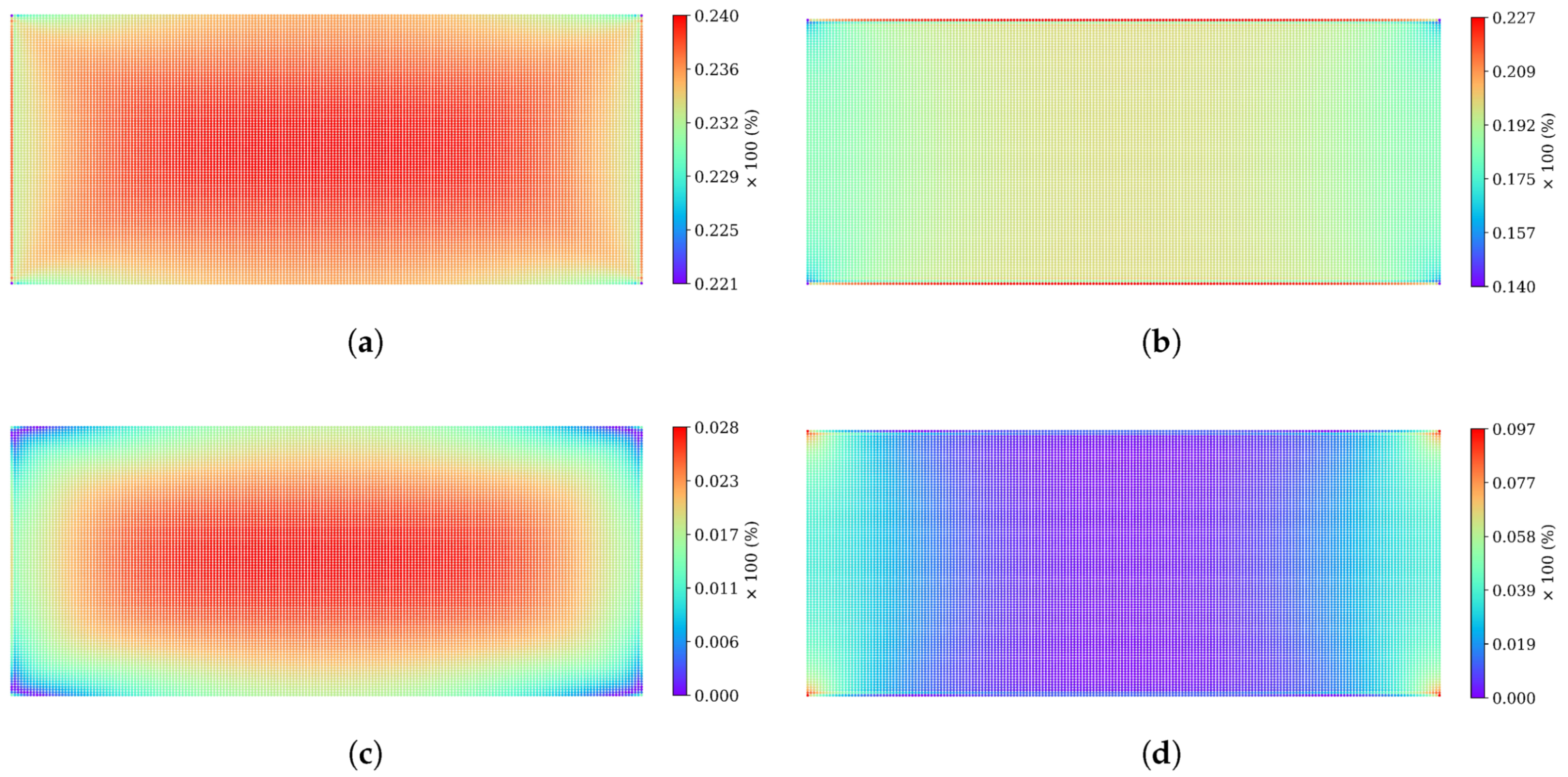
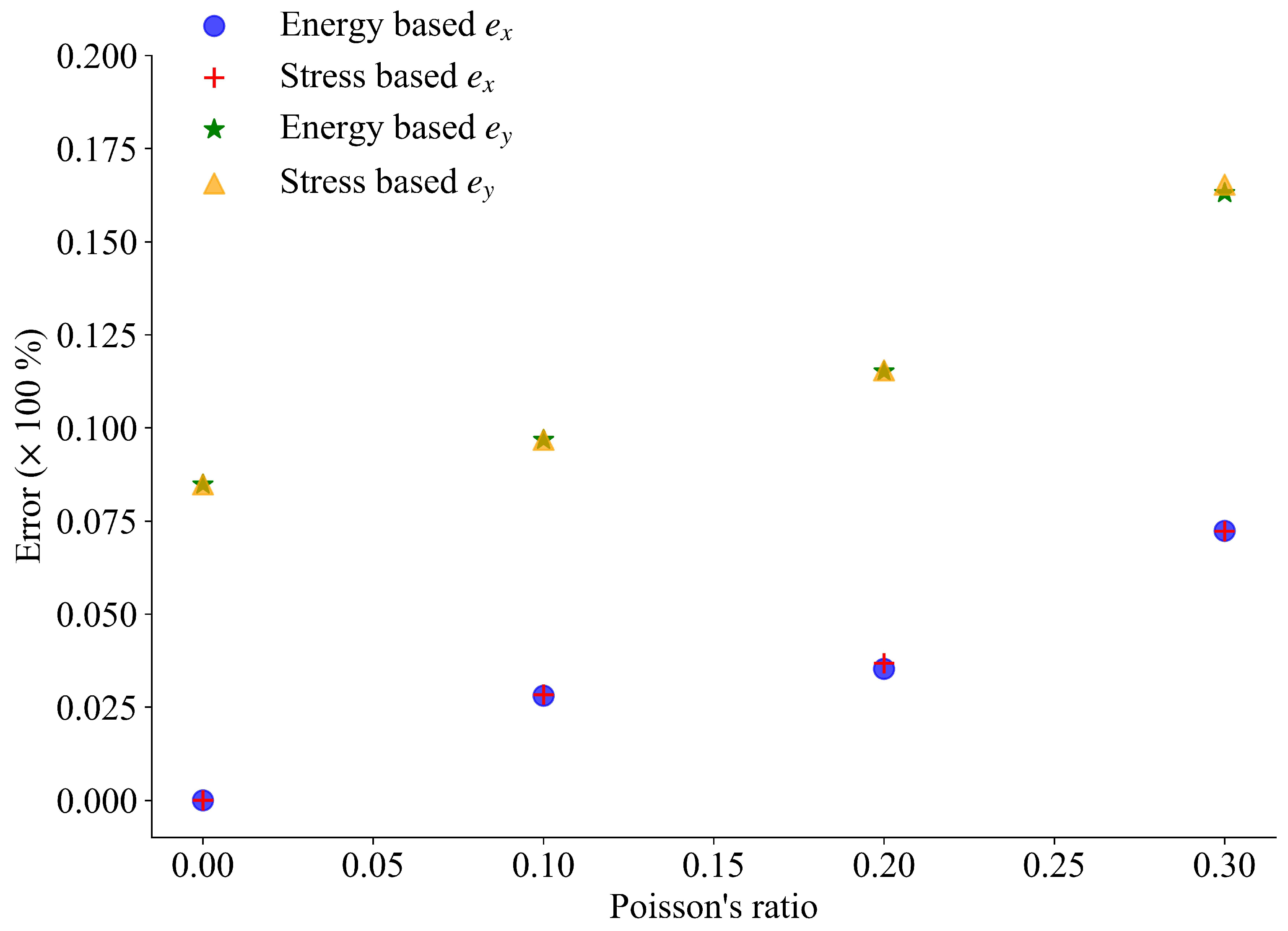
• The proposed stress-based correction method effectively mitigates skin effects. The absolute errors introduced are of the same magnitude as those calculated using the energy-based correction method. The accuracy of node displacement compared to analytical displacements improves as Poisson’s ratio decreases, indicating the correction’s dependence on the sample’s Poisson’s ratio.
• Before correction, PD equations using bond strain conditions yield lower absolute displacement errors along the loading axis compared to those using bond deformation. However, after correction, both methods produce similar errors along this axis. Along the other axis, although the absolute errors are higher before correction for PD equations formulated using bond deformation, they tend to be lower near the boundary after correction compared to those formulated using bond strain conditions. This implies that the PD model developed based on bond deformation could potentially be more effective compared to the model derived from bond strain.
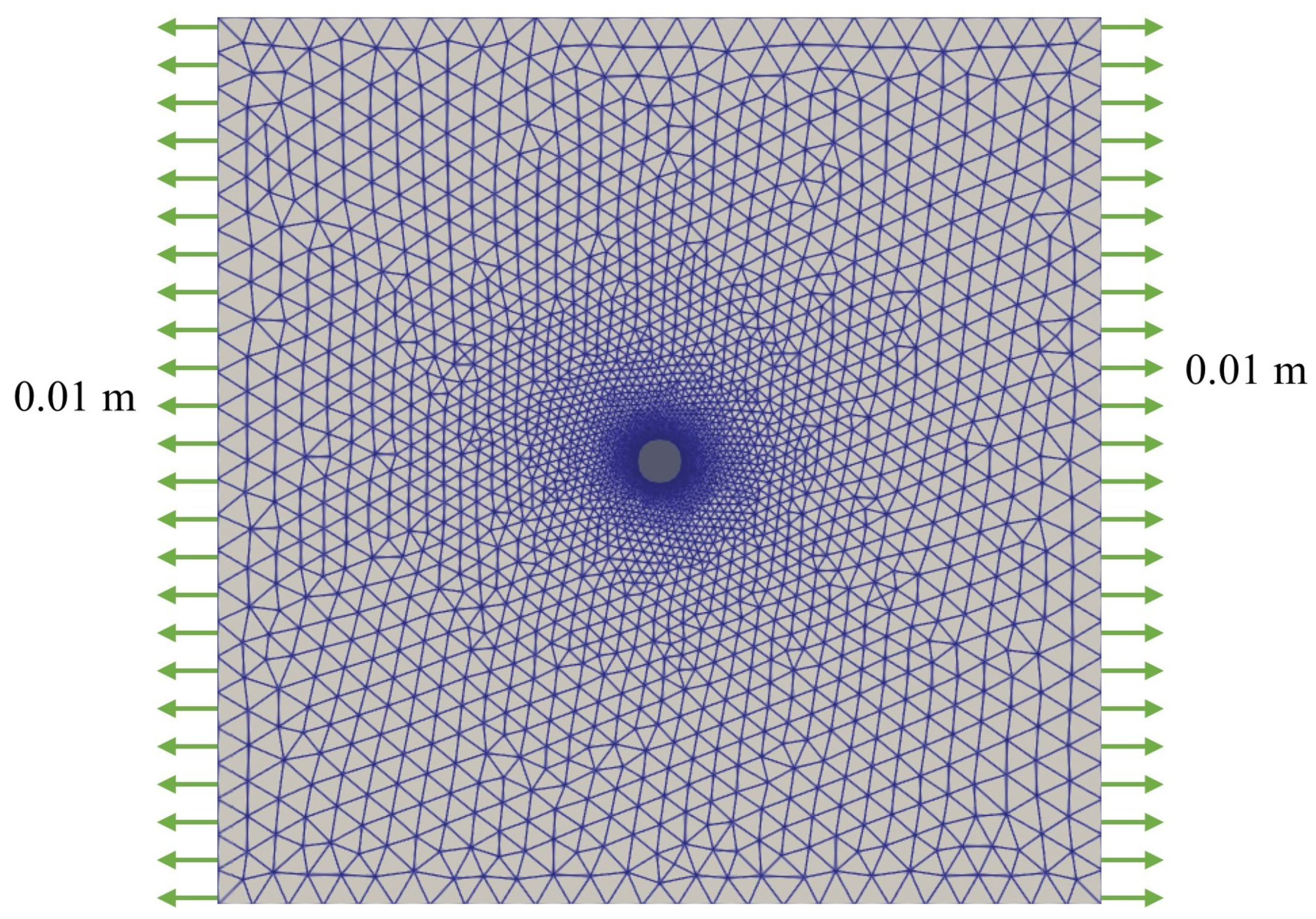
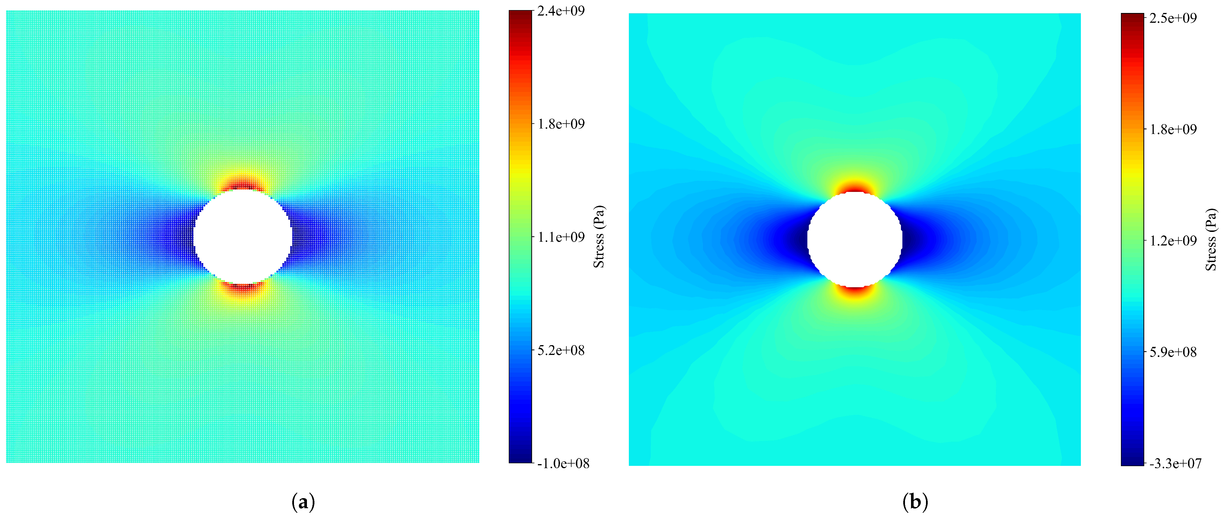
• Deformation-based PD has proven effective in accurately capturing the stress concentration factor, demonstrating its potential for application in modeling complex geometries.
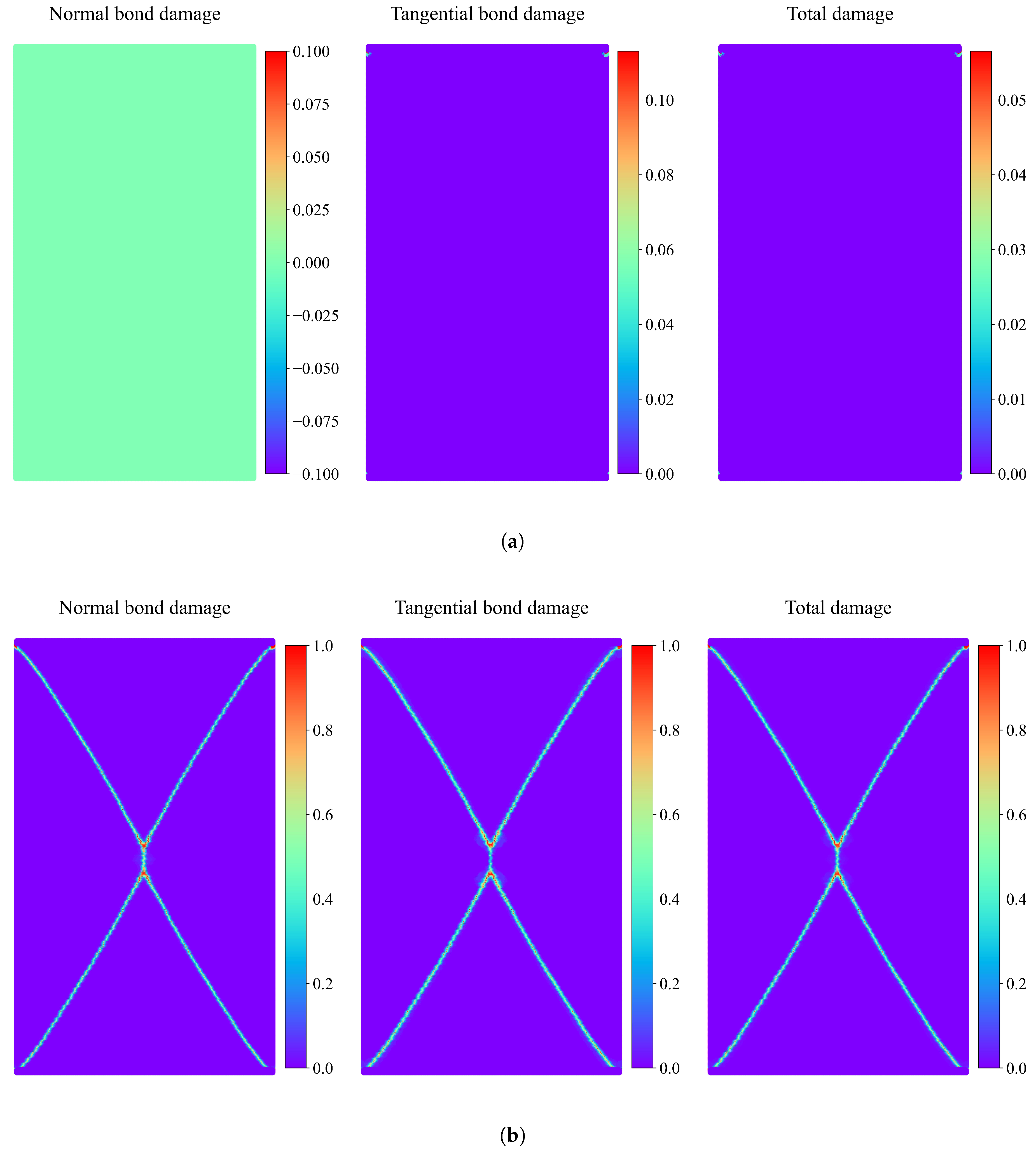
• A mixed-mode failure criterion is derived for deformation-based PD. X-shaped conjugate shear failure is observed in granite specimens, resembling the failure of intact rocks under uniaxial compression testing. Additionally, tangential bond failure occurs before normal bond failure in the uniaxial test.

Although the practical applications of the proposed bond deformation-based peridynamic model have yet to be fully explored, we believe that this approach holds significant potential for improving the simulation of fracture processes, damage evolution, and failure prediction in brittle materials. Despite the promising applicability in real-world engineering, it also has inherent limitations. Future work could involve extending the model to 3D problems, improving the model to incorporate a broader range of Poisson’s ratios to represent materials more accurately, introducing material heterogeneity in the model to simulate realistic materials, and implementing multi-threading strategies to enhance computational efficiency.

References

1. Silling, S.A. Reformulation of elasticity theory for discontinuities and long-range forces. J. Mech. Phys. Solids 2000, 48, 175–209. [Google Scholar] [CrossRef]
2. Silling, S.A.; Askari, E. A meshfree method based on the peridynamic model of solid mechanics. Comput. Struct. 2005, 83, 1526–1535. [Google Scholar] [CrossRef]
3. Ai, D.; Zhao, Y.; Wang, Q.; Li, C. Crack propagation and dynamic properties of coal under SHPB impact loading: Experimental investigation and numerical simulation. Theor. Appl. Fract. Mech. 2020, 105, 102393. [Google Scholar] [CrossRef]
4. Silling, S.A.; Epton, M.; Weckner, O.; Xu, J.; Askari, E. Peridynamic States and Constitutive Modeling. J. Elast. 2007, 88, 151–184. [Google Scholar] [CrossRef]
5. Dimola, N.; Coclite, A.; Fanizza, G.; Politi, T. Bond-based peridynamics, a survey prospecting nonlocal theories of fluid-dynamics. Adv. Contin. Discret. Model. 2022, 2022, 60. [Google Scholar] [CrossRef]
6. Fallah, A.S.; Giannakeas, I.N.; Mella, R.; Wenman, M.R.; Safa, Y.; Bahai, H. On the Computational Derivation of Bond-Based Peridynamic Stress Tensor. J. Peridyn. Nonlocal Model. 2020, 2, 352–378. [Google Scholar] [CrossRef]
7. Battistini, A.; Haynes, T.A.; Jones, L.; Wenman, M.R. Bond-based peridynamics model of 3-point bend tests of ceramic-composite interfaces. J. Am. Ceram. Soc. 2024, 107, 6004–6018. [Google Scholar] [CrossRef]
8. Silling, S.A. Introduction to peridynamics. In Handbook of Peridynamic Modeling; Bobaru, F., Foster, J.T., Geubelle, P.H., Silling, S.A., Eds.; Chapman and Hall/CRC: New York, NY, USA, 2016; pp. 63–98. [Google Scholar]
9. Gerstle, W.; Sau, N.; Silling, S. Peridynamic modeling of concrete structures. Nucl. Eng. Des. 2007, 237, 1250–1258. [Google Scholar] [CrossRef]
10. Wang, Y.; Zhou, X.; Shou, Y. The modeling of crack propagation and coalescence in rocks under uniaxial compression using the novel conjugated bond-based peridynamics. Int. J. Mech. Sci. 2017, 128–129, 614–643. [Google Scholar] [CrossRef]
11. Wang, Y.; Zhou, X.; Wang, Y.; Shou, Y. A 3-D conjugated bond-pair-based peridynamic formulation for initiation and propagation of cracks in brittle solids. Int. J. Solids Struct. 2018, 134, 89–115. [Google Scholar] [CrossRef]
12. Huang, X.; Li, S.; Jin, Y.; Yang, D.; Su, G.; He, X. Analysis on the influence of Poisson’s ratio on brittle fracture by applying uni-bond dual-parameter peridynamic model. Eng. Fract. Mech. 2019, 222, 106685. [Google Scholar] [CrossRef]
13. Gao, C.; Zhou, Z.; Li, L.; Li, Z.; Zhang, D.; Cheng, S. Strength reduction model for jointed rock masses and peridynamics simulation of uniaxial compression testing. Geomech. Geophys. Geo-Energy Geo-Resour. 2021, 7, 1–21. [Google Scholar] [CrossRef]
14. Yang, S.Q.; Yang, Z.; Zhang, P.C.; Tian, W.L. Experiment and peridynamic simulation on cracking behavior of red sandstone containing a single non-straight fissure under uniaxial compression. Theor. Appl. Fract. Mech. 2020, 108, 102637. [Google Scholar] [CrossRef]
15. Ha, Y.D.; Lee, J.; Hong, J.W. Fracturing patterns of rock-like materials in compression captured with peridynamics. Eng. Fract. Mech. 2015, 144, 176–193. [Google Scholar] [CrossRef]
16. Yaghoobi, A.; Chorzepa, M.G. Fracture analysis of fiber reinforced concrete structures in the micropolar peridynamic analysis framework. Eng. Fract. Mech. 2017, 169, 238–250. [Google Scholar] [CrossRef]
17. Du, W.; Fu, X.; Sheng, Q.; Chen, J.; Du, Y.; Zhang, Z. Study on the failure process of rocks with closed fractures under compressive loading using improved bond-based peridynamics. Eng. Fract. Mech. 2020, 240, 107315. [Google Scholar] [CrossRef]
18. Zhou, Z.; Li, Z.; Gao, C.; Zhang, D.; Wang, M.; Wei, C.; Bai, S. Peridynamic micro-elastoplastic constitutive model and its application in the failure analysis of rock masses. Comput. Geotech. 2021, 132, 104037. [Google Scholar] [CrossRef]
19. Li, S.; Lu, H.; Jin, Y.; Sun, P.; Huang, X.; Bie, Z. An improved unibond dual-parameter peridynamic model for fracture analysis of quasi-brittle materials. Int. J. Mech. Sci. 2021, 204, 106571. [Google Scholar] [CrossRef]
20. Feng, K.; Zhou, X.P. Peridynamic simulation of the mechanical responses and fracturing behaviors of granite subjected to uniaxial compression based on CT heterogeneous data. Eng. Comput. 2023, 39, 1–23. [Google Scholar] [CrossRef]
21. Diana, V.; Casolo, S. A bond-based micropolar peridynamic model with shear deformability: Elasticity, failure properties and initial yield domains. Int. J. Solids Struct. 2019, 160, 201–231. [Google Scholar] [CrossRef]
22. Madenci, E.; Barut, A.; Phan, N. Bond-based peridynamics with stretch and rotation kinematics for opening and shearing modes of fracture. J. Peridyn. Nonlocal Model. 2021, 3, 211–254. [Google Scholar] [CrossRef]
23. Chen, Z.; Ju, J.W.; Su, G.; Huang, X.; Li, S.; Zhai, L. Influence of micro-modulus functions on peridynamics simulation of crack propagation and branching in brittle materials. Eng. Fract. Mech. 2019, 216, 106498. [Google Scholar] [CrossRef]
24. Kilic, B.; Madenci, E. Structural stability and failure analysis using peridynamic theory. Int. J. Non-Linear Mech. 2009, 44, 845–854. [Google Scholar] [CrossRef]
25. Kilic, B.; Madenci, E. Prediction of crack paths in a quenched glass plate by using peridynamic theory. Int. J. Fract. 2009, 156, 165–177. [Google Scholar] [CrossRef]
26. Madenci, E.; Oterkus, E. Peridynamic Theory and Its Applications; Springer: New York, NY, USA, 2014. [Google Scholar] [CrossRef]
27. Shen, S.; Yang, Z.; Han, F.; Cui, J.; Zhang, J. Peridynamic modeling with energy-based surface correction for fracture simulation of random porous materials. Theor. Appl. Fract. Mech. 2021, 114, 102987. [Google Scholar] [CrossRef]
28. Kilic, B.; Madenci, E. Coupling of peridynamic theory and the finite element method. J. Mech. Mater. Struct. 2010, 5, 707–733. [Google Scholar] [CrossRef]
29. Macek, R.W.; Silling, S.A. Peridynamics via finite element analysis. Finite Elem. Anal. Des. 2007, 43, 1169–1178. [Google Scholar] [CrossRef]
30. Liu, Y.; Han, F.; Zhang, L. An extended fictitious node method for surface effect correction of bond-based peridynamics. Eng. Anal. Bound. Elem. 2022, 143, 78–94. [Google Scholar] [CrossRef]
31. Mitchell, J.; Silling, S.; Littlewood, D. A position-aware linear solid constitutive model for peridynamics. J. Mech. Mater. Struct. 2015, 10, 539–557. [Google Scholar] [CrossRef]
32. Le, Q.; Bobaru, F. Surface corrections for peridynamic models in elasticity and fracture. Comput. Mech. 2018, 61, 499–518. [Google Scholar] [CrossRef]
33. Gao, H.; Klein, P. Numerical simulation of crack growth in an isotropic solid with randomized internal cohesive bonds. J. Mech. Phys. Solids 1998, 46, 187–218. [Google Scholar] [CrossRef]
34. Zhang, Z.; Ge, X. Micromechanical consideration of tensile crack behavior based on virtual internal bond in contrast to cohesive stress. Theor. Appl. Fract. Mech. 2005, 43, 342–359. [Google Scholar] [CrossRef]
35. Zhennan, Z.; Xiurun, G. Micromechanical modelling of elastic continuum with virtual multi-dimensional internal bonds. Int. J. Numer. Methods Eng. 2006, 65, 135–146. [Google Scholar] [CrossRef]
36. Boresi, A.P.; Chong, K.; Lee, J.D. Elasticity in Engineering Mechanics; John Wiley & Sons: Hoboken, NJ, USA, 2010. [Google Scholar]
37. Ha, Y.D.; Bobaru, F. Characteristics of dynamic brittle fracture captured with peridynamics. Eng. Fract. Mech. 2011, 78, 1156–1168. [Google Scholar] [CrossRef]
38. Seleson, P.; Parks, M.L.; Gunzburger, M.; Lehoucq, R.B. Peridynamics as an upscaling of molecular dynamics. Multiscale Model. Simul. 2009, 8, 204–227. [Google Scholar] [CrossRef]
39. Li, J.; Li, S.; Lai, X.; Liu, L. Peridynamic stress is the static first Piola–Kirchhoff Virial stress. Int. J. Solids Struct. 2022, 241, 111478. [Google Scholar] [CrossRef]
40. Lutz, M. Programming Python: Powerful Object-Oriented Programming; O’Reilly Media, Inc.: Sebastopol, CA, USA, 2010. [Google Scholar]
41. Behnel, S.; Bradshaw, R.; Citro, C.; Dalcin, L.; Seljebotn, D.S.; Smith, K. Cython: The Best of Both Worlds. Comput. Sci. Eng. 2011, 13, 31–39. [Google Scholar] [CrossRef]
42. Sauvé, R.; Metzger, D. Advances in dynamic relaxation techniques for nonlinear finite element analysis. J. Press. Vessel Technol.-Trans. 1995, 117, 170–176. [Google Scholar] [CrossRef]
43. Ha, Y.D.; Bobaru, F. Studies of dynamic crack propagation and crack branching with peridynamics. Int. J. Fract. 2010, 162, 229–244. [Google Scholar] [CrossRef]
44. Zhu, Q.Z.; Ni, T. Peridynamic formulations enriched with bond rotation effects. Int. J. Eng. Sci. 2017, 121, 118–129. [Google Scholar] [CrossRef]
Figure 1. Interaction of a node in a peridynamic framework.
Buildings 15 01931 g001
Figure 2. Interaction between two particles in PD.
Buildings 15 01931 g002
Figure 3. Normal and rotational bonds in modified VIB. (a) 3D, (b) 2D.
Buildings 15 01931 g003
Figure 4. Illustration of normal and tangential displacement between two nodes in PD.
Buildings 15 01931 g004
Figure 5. Incomplete horizon for particles located at the edges of a domain.
Buildings 15 01931 g005
Figure 6. A PD node interacting in a hypothetical infinite subdomain.
Buildings 15 01931 g006
Figure 7. Relation between node density and computed stress for the central node in the infinite domain.
Buildings 15 01931 g007
Figure 8. Flowchart illustrating the implementation procedure for the PD equations used in this study.
Buildings 15 01931 g008
Figure 9. Rectangular plate subjected to uniaxial tensile loading.
Buildings 15 01931 g009
Figure 10. Errors in measurements of u x and u y obtained from the stress-based method (Poisson’s ratio 0.1). (a) e x before correction. (b) e y before correction. (c) e x after correction. (d) e y after correction.
Buildings 15 01931 g010
Figure 11. Comparison of errors between stress-based and energy-based methods ( e x and e y represent maximum errors measured in x and y displacements, respectively).
Buildings 15 01931 g011
Figure 12. The plate with the hole subjected to displacement boundary conditions.
Buildings 15 01931 g012
Figure 13. Stress distribution ( σ x x ) in the vicinity of the hole. (a) PD, (b) FEM.
Buildings 15 01931 g013
Figure 14. Comparison of FEM and PD predictions of displacement along the horizontal and vertical centerlines of the hole. (a) x-displacement along the horizontal centerline, (b) y-displacement along the vertical centerline.
Buildings 15 01931 g014
Figure 15. Dimensions of the granite specimen (with boundary layers) used for the uniaxial compression test.
Buildings 15 01931 g015
Figure 16. The stress–strain curve for the tested granite specimen (CT-based data for the 3D simulation were reproduced from Feng and Zhou [20].
Buildings 15 01931 g016
Figure 17. Evolution of damage and final failure pattern of the specimen. (a) Evolution of bond failures in the specimen, showing that tangential bonds fail earlier than normal bonds. (b) Final failure pattern of the specimen.
Buildings 15 01931 g017
Figure 18. Comparison between the final failure pattern in this study and the reference study. (a) This study, (b) the reference study (the schematic diagram is reproduced from Feng and Zhou [20]).
Buildings 15 01931 g018
Figure 19. Errors in measurements of u x and u y before correction (Poisson’s ratio 0.2). (a) e x obtained from bond deformation; (b) e y obtained from bond deformation; (c) e x obtained from the bond stretch; (d) e y obtained from the bond stretch.
Buildings 15 01931 g019
Figure 20. Errors in measurements of u x and u y after correction (Poisson’s ratio 0.2). (a) e x obtained from bond deformation; (b) e y obtained from bond deformation; (c) e x obtained from the bond stretch; (d) e y obtained from the bond stretch.
Buildings 15 01931 g020