Article

Two-Scale Physics-Informed Neural Networks for Structural Dynamics Parameter Inversion: Numerical and Experimental Validation on T-Shaped Tower Health Monitoring

by
Xinpeng Liu
1,2,
Xuemei Zhang
1,
Yongli Zhong
1,2,
Zhitao Yan
1,2,3,* and
Yu Hong
1,*
1
School of Civil and Hydraulic Engineering, Chongqing University of Science and Technology, Chongqing 401331, China
2
Chongqing Key Laboratory of Disaster Prevention and Reduction in Power Transmission Engineering, Chongqing 401331, China
3
Chongqing Industry and Trade Polytechnic, Chongqing 401331, China
*
Authors to whom correspondence should be addressed.
Buildings 2025, 15(11), 1876; https://doi.org/10.3390/buildings15111876
Submission received: 17 April 2025 / Revised: 23 May 2025 / Accepted: 27 May 2025 / Published: 29 May 2025

Abstract

We present a two-scale physics-informed neural network (TSPINN) algorithm to address structural parameter inversion problems involving small parameters. The algorithm’s core mechanism directly embeds small parameters into the neural network architecture. By constructing a two-scale neural network architecture, this approach enables the simultaneous analysis of structural dynamic responses and local parameter perturbation effects, which effectively addresses challenges posed by high-frequency oscillations and parameter sensitivity. Numerical experiments demonstrate that TSPINNs significantly improve prediction accuracy and convergence speed compared to conventional physics-informed neural networks (PINNs) and maintain robustness in high-stiffness scenarios. The T-shaped tower shaking table test results confirm that the model’s identification errors for stiffness reduction coefficients and mass parameters remain below 10% under lower noisy conditions, demonstrating high precision and strong generalization capability for multi-damage scenarios and random load excitations.

1. Introduction

Structural health monitoring constitutes the cornerstone of modern engineering safety, providing a framework for lifecycle management of critical infrastructure such as bridges and aerospace systems. Parameter inversion constitutes the methodological foundation of this approach, enabling damage identification and condition assessment through inverse analysis of key dynamic parameters such as stiffness and damping ratios. Conventional numerical methods and data-driven models often encounter dimensionality disasters and ill-posed equations, resulting in significant accuracy degradation and efficiency loss under complex operational conditions and noise interference. In recent years, deep learning technology has significantly advanced parameter identification techniques by integrating physical laws with data-driven paradigms, particularly in structural damage assessment and dynamic load recognition.
The development of structural parameter inversion methods has witnessed a significant evolution from traditional analytical models to contemporary data-driven approaches. While early methodologies demonstrated effectiveness in specific scenarios, their limitations are increasingly revealed when applied to complex engineering applications.
Conventional structural parameter identification approaches rely on analytical solutions and optimization algorithms but face significant challenges in complex engineering applications. In the context of noise sensitivity, while the two-stage Bayesian inversion framework proposed by Yuen et al. [1] enhances computational efficiency through modal screening, the method’s dependence on prior distributions leads to substantial recognition errors in non-Gaussian noise environments [2]. Lai et al. [3] achieved 80% parameter dimension reduction through L1 regularization in their sparse identification system, though constrained by predefined candidate function libraries, particularly for novel material parameter identification. Furthermore, these methods face challenges in time-varying parameter analysis: Banerjee et al. [4] demonstrated that the auto-regularization pseudo-time advancing method shows poor convergence and requires more iteration during material softening parameter identification.
To address traditional methods’ limitations, deep learning technology has advanced structural health monitoring applications. Nadith [5] pioneered the application of autoencoder models to steel frame damage identification, effectively addressing high-dimensional nonlinear feature extraction through layer-wise pre-training coupled with global fine-tuning strategies. For microscopic damage detection, constructed by Guo et al. [6] developed the SE-U-Net model with attention mechanisms, achieving 98.48% accuracy in pixel-level concrete microcracks identification. Hu et al. [7] proposed a complex exponential signal decomposition method that achieves the simultaneous identification of damping ratios and stiffness coefficients with relative errors within 5%, though limited by low-frequency dense mode resolution, with errors increasing to 15% during the identification of frequency-similar parameters due to spectral overlap. Bao et al. [8] developed a transfer learning framework for bridge elastic modulus identification using finite element simulation data, though its accuracy markedly decreases for time-varying parameters. However, the multi-source excitation identification method’s error escalates significantly with increasing excitation sources [9]. Shu et al. [10] integrated the learning without forgetting (LWF) method into ResNet-34 architecture, creating the Continuous learning damage recognition model (CLDRM) that effectively mitigates catastrophic forgetting in traditional models.
Lu et al. [11] proposed DeepONet for solving nonlinear PDE via operator learning, while the Fourier neural operator (FNO) proposed by Li et al. [12] significantly enhanced high-dimensional flow field simulation efficiency. Xu et al. [13] applied transfer learning to address structural inversion problems across varying load scenarios, and Penwarden [14] implemented meta-learning to optimize parameter initialization in physics-informed neural networks (PINNs). Nevertheless, data-driven approaches like LordNet (Shi et al. [15]) require extensive simulation data and exhibit limited generalizability. Wang et al. [16,17] demonstrated that insufficient training data in long-term dynamic simulations cause significant accuracy degradation, highlighting the urgent need to improve interpretability and extrapolation capability through embedded physical laws.
Physics-informed neural networks (PINNs) proposed by Raissi et al. [18,19] enable unified solutions for forward/inverse problems through the synergistic integration of physical laws with automatic differentiation [20]. The paradigm’s core innovation involves embedding partial differential equation residuals into loss function [21,22,23,24,25,26], providing both data efficiency and physical consistency while overcoming the curse of dimensionality and eliminating mesh generation requirements [27], thereby establishing a foundational methodology for subsequent research.
The physics-informed neural network (PINN) methodology continues to evolve, driving interdisciplinary applications through the integration of data-driven models with physical priors. This integration has enabled transformative developments across civil engineering [28,29,30,31], fluid mechanics [32,33,34,35,36,37,38,39,40], biomedicine [41,42], and energy systems [43,44]. In parameter inversion studies: Rucker et al. [45] developed physics-informed deep learning for fault friction parameter identification; Liu et al. [46] integrated physical principles with data-driven strategies for moving load characterization; Nagao et al. [47] applied physics-informed machine learning to quantify reservoir connectivity parameters (transmissibility, permeability distribution, regional connectivity coefficients); and Wang et al. [48] established a mesh-based PINN framework (M-PINN) for the inverse analysis of material properties and boundary conditions in linear elasticity problems.
Despite well-established applications of physics-informed neural networks (PINNs), persistent challenges remain in engineering systems with multi-scale characteristics and extreme parameter ranges. Jin et al. [49] tackled multi-scale challenges through asymptotic-preserving neural networks (APNN) using explicit asymptotic expansions; however, this method introduces computational complexity and solution variability stemming from decomposition strategies and truncation term selection. This work introduces a two-scale physics-informed neural network (TSPINN) that integrates small-scale parameters as embedded network inputs, enabling implicit multi-scale feature learning while maintaining implementation simplicity. Through four numerical validation cases, we systematically evaluate TSPINNs’ accuracy and robustness, with particular focus on damage parameter inversion performance under minor parametric variations using a T-shaped tower structure. This approach ultimately seeks to transcend traditional method limitations and deliver an efficient intelligent solution for structural health monitoring.
The main contributions of this paper are summarized as follows:
(1)
In the network architecture, introducing scale parameters at the input layer breaks the limitation of single scale, achieving the decoupling of two-scale features and the fusion of cross-scale information.
(2)
At the level of physical modeling, we define the stiffness-to-mass ratio as a characteristic scale parameter, construct scale auxiliary variables, establish a universal scale correlation mechanism, and break through the limitations of traditional methods.
(3)
The proposed TSPINN framework integrates finite element principles with two-scale physics-informed learning to achieve damage localization and stiffness/mass quantification of T-shaped tower structures under dynamic excitation. By incorporating finite element principles, it addresses the limitations of traditional physics-informed neural networks in scenarios involving small parameters and single partial differential equations, demonstrating superior performance in complex structural contexts.
The paper is organized as follows: Section 2 details the architecture of two-scale physics-informed neural networks (TSPINNs), with numerical validations across four benchmark cases demonstrating method accuracy. Section 3 presents engineering applications through T-shaped tower case studies. First, forward analysis validates the algorithm’s mechanical response prediction capability. Second, experimentally acquired dynamic responses from shaking table tests are utilized for parameter inversion within the TSPINN framework, conducting systematic verification of robustness and engineering applicability. Section 4 synthesizes key findings and proposes future research trajectories.

2. Methodology

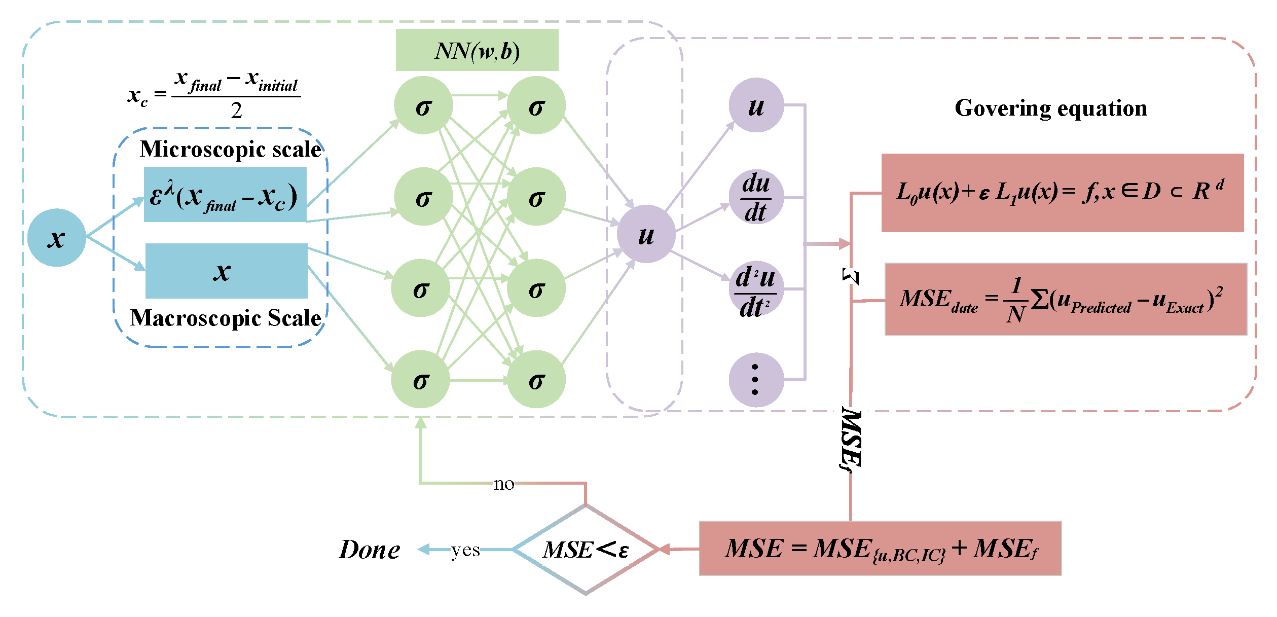
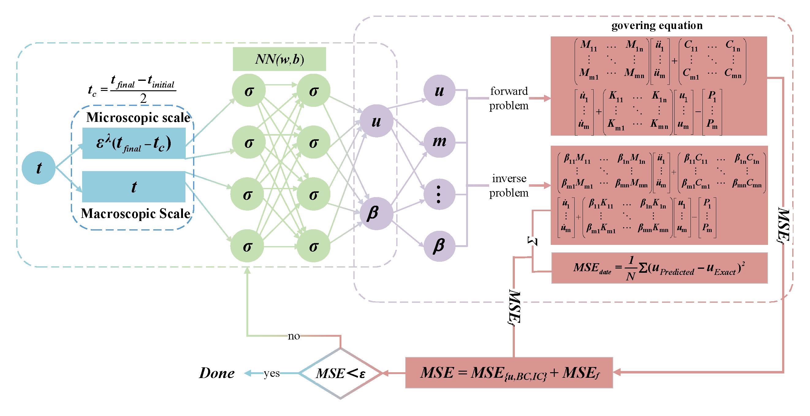
2.1. Two-Scale Physics-Informed Neural Network Principles

Two-scale physics-informed neural networks (TSPINNs) are a deep learning framework designed for partial differential equations (PDEs) with small parameters. The partial differential equations with small parameters are as follows:
L 0 u ( x ) + ε L 1 u ( x ) = f , x D R d
where
  • L 0 is the dominant differential operator, representing the main physical behaviors or macrodynamic characteristics of the system.
  • ε is a dimensionless small parameter ( 0 < ε 1 ), reflecting the relative strength of secondary effects or micro-scale disturbances.
  • L 1 serves as a secondary differential operator (perturbation operator), typically describing microscale corrections induced by viscous, diffusive, or nonlinear effects. Although its overall contribution is suppressed by ε, it may dominate the form of the solution in localized regions such as boundary layers, shock waves, or resonance bands.
  • f is the source term or external forcing term that drives the dynamic response of the system.
To address complex characteristics such as boundary layers, internal layers, and high-frequency oscillations caused by small parameters, the core of TSPINNs lies in directly incorporating small parameters into the neural network to construct a two-scale neural network. The structure of the network is as follows:
u ( x ) = ω ( x ) N ( x , ε λ x x c , ε λ )
The function ω ( x ) serves as a boundary condition adaptation function (such as ω x = 1 or simple functions that satisfy Dirichlet conditions), and the network employs a fully connected architecture with the Tanh activation function.
The input layer of TSPINNs (Figure 1) comprises macro- and micro-scale variables. The macro-scale (primary scale) corresponds to the original partial differential equation variables, capturing the problem’s global behavior, while the micro-scale addresses fine-scale features governed by small parameters, corresponding to high-frequency components present in the solution. At this scale, solution variations exhibit pronounced gradients, experiencing rapid changes within localized spatial domains. The architecture typically incorporates three distinct inputs corresponding to two-scale variables:
(a)
Original input variable (x): the primary variable in the partial differential equation representing the original spatial or temporal variable.
(b)
Scaling variables ( ε λ x x c , ( λ R ) ): The computational domain D is characterized by its centroid x c , and a small parameter ε governing the equation, which serves to resolve multiscale features in the governing equation’s solution profile. Through the strategic coupling of the spatial coordinate x with the scaled variables ε λ x x c , the architecture explicitly targets microscale variations while maintaining macroscale solution fidelity.
(c)
Scale parameter ( ε λ ): This parameter is designed to assist the network in feature capture across different scales, thereby effectively addressing multi-scale issues.
Under the framework of PINNs, the neural network solution is obtained by minimizing the loss function of residuals. The loss function of the considered problem (1) at the continuous level is as follows:
L t o t a l = L r e s i d u a l + L b o u n d a r y + L i n i t i a l + L g r a d i e n t
The respective residual:
L r e s i d u a l = 1 N c i = 1 N c L 0 u ( x i ) + ε L 1 u ( x i ) f ( x i ) 2
L b o u n d a r y = α N b j = 1 N b u ( x j ) g ( x j ) 2
L i n i t i a l = β N o k = 1 N o u ( 0 , x k ) u 0 ( x k ) 2
L g r a d i e n t = α 1 N c i = 1 N c u ( x i ) 2
α 1 , β 0 , α 1 0 , x i i = 1 N c is the configuration point of D within the domain. x j i = 1 N b is the boundary sampling point.
This article employs an ADAM optimizer to train the parameters of the neural network, utilizing a stepwise training approach during the training process. The TSPINN architecture is illustrated in Figure 1, and the algorithm is detailed in Algorithm 1 (Pseudocode for the TSPINN algorithm embedded with physical information) and Algorithm 2 (Pseudocode for the TSPINN algorithm embedded with physical information).
Compared to traditional PINNs, TSPINNs process the input into two components, namely macroscopic and microscopic, thus enhancing the network’s ability to capture solutions at the observational scale.
Algorithm 1: Successive training of two-scale neural networks for PDEs with small parameters
Data: 
Training set, adaptive learning rates, ϵ and other parameters from the PDE
Result: 
Optimized weights and bias of the neural networks
Step 1.
Pick a large ε 0 if ε is small; otherwise set ε 0 = ε . Train optimized weights and bias of the neural networks with the scale 1 and ε 0 1 2 .
Step 2.
Repeat Step 1 once if necessary, e.g., 10 ε is still small.
Step 3.
Compute the gradients of the trained neural networks in Steps 1 & 2 on a different set of sampling points, in addition to training points.
Step 4.
(Adaptive sampling). Find the first few points where the norm of the gradient is large.
Add a few more points.
Step 5.
(Fine-tuning). Use Adam with a smaller learning rate to further optimize the weights and biases.
Step 6.
Stop the process if the iteration attains the maximal epoch number specified.
Algorithm 2: Algorithm embedded with TSPINNs
Input:
Randomly scatter dots in the linear time domain and enter t;
 Introduce scale parameters x , ε λ x f i n a l x c , ε λ ;
Net:
The number of network layers L , the number of neurons m in each hidden layer, the activation function Tanh, and the learning rate α ;
Output: 
the displacement response of the structure;
Step1:
Construct a fully connected neural network and initialize the neural network parameter θ ;
Step2:
Constructed loss function L ( x ) : initial conditional loss and ordinary differential equation loss;
Step3:
Start training;
Step4:
I t m a x > I t or L ( x ) < threshold ϑ :
Calculating Network Loss: M S E = w 0 M S E u , B C , I C + w f M S E f
Calculate the gradient of network parameters: J ( θ 1 , θ 2 θ i θ n ) j
Update network parameters:   θ j = θ j α J ( θ 1 , θ 2 θ i θ n ) θ j
End
 

2.2. Numerical Experiments

In this section, the sensitivity characteristics of small parameter changes to large derivative solutions are investigated through case studies. The computer configuration for network training is an Intel Core i7–13700KF CPU, a RAM of 64 GB (Intel, Mountain View, CA, USA), and a NVIDIA GeForce RTX 4090 GPU (NVIDIA, Santa Clara, CA, USA). The required training times were 1.5 h and 4 h, as shown in Section 2.2 and Section 3, respectively.
Without stating otherwise, we adopt the adaptive learning rate scheduler, the uniform distribution for collocation points, and the tanh activation function, as listed in Table 1.
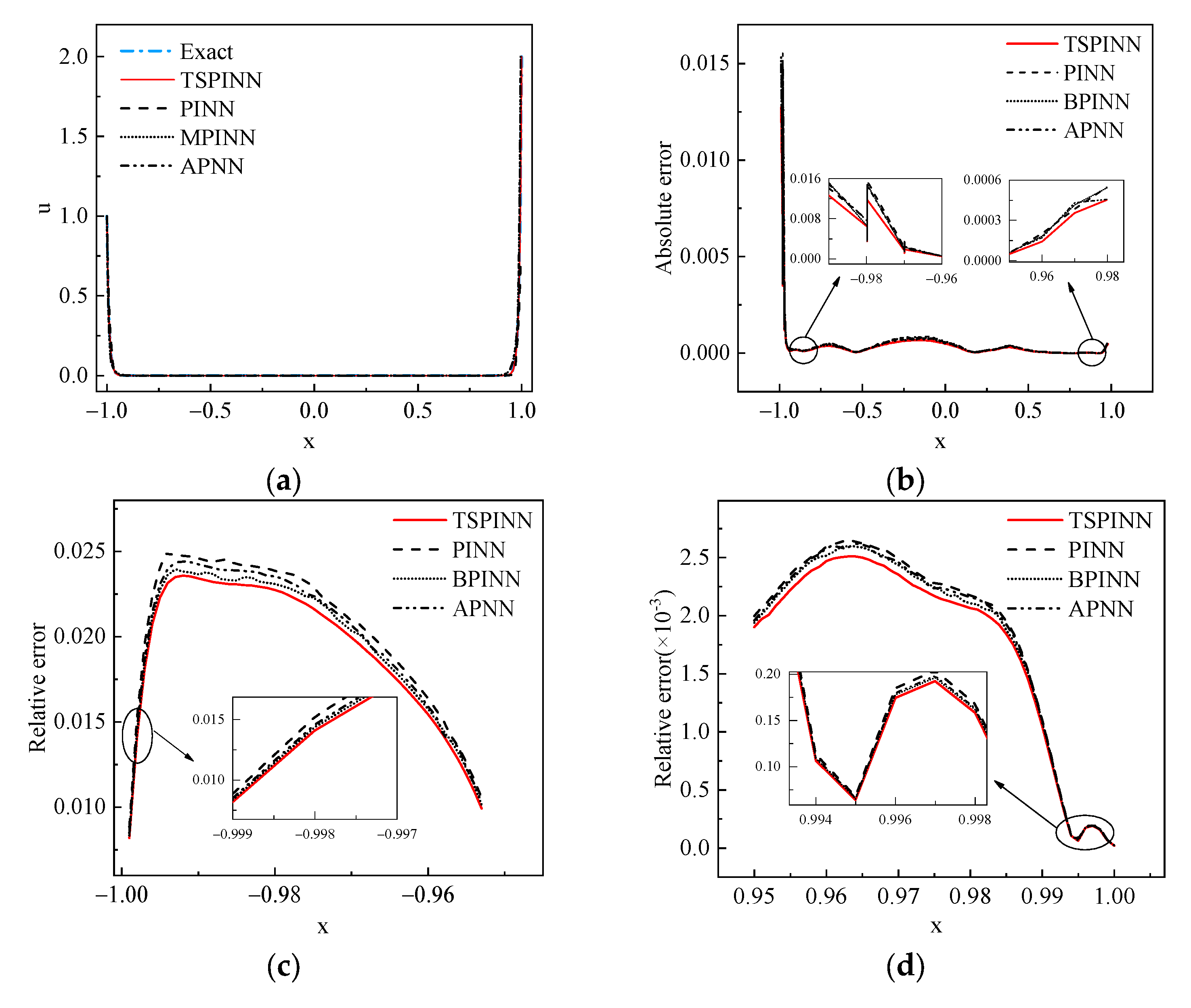
  • Example 1 (1D ODE with one boundary layer):
ε u + 2 u = 3 , u 0 = 0 ,   u 1 = 0
The exact solution to this problem is
u x = 3 2 x exp 2 1 x ε e x p ( 2 / ε ) 1 e x p ( 2 / ε )
The solution has a boundary layer at x = 1 . When ε = 10 2 , the ODE equation is solved using TSPINNs, with the results shown in Figure 2. From Figure 2, it can be observed that compared to other improved PINNs, the solution obtained by TSPINNs closely aligns with the exact solution, where the maximum relative error at the boundary layer x = 1 is only 0.15. In the figure, M-PINN is a mesh-based physics-informed neural network (M-PINN) [48], while APNN is an asymptotic-preserving neural network (APNN) [49].
  • Example 2 (1D ODE with two boundary layer):
ε u x u u = 0 , 1 < x < 1 , u 1 = 1 ,   u 1 = 2
The exact solution to this problem is
exp x 2 1 2 ε E r f x 2 ε + 3 E r f 1 2 ε 2 E r f 1 2 ε , E r f z = 2 π 0 z e x p ( t 2 ) d t
The solution has two boundary layers, at x = ± 1 . Figure 3 shows the results of solving the equations using TSPINNs for   ε = 10 2 . It can be observed from the figure that compared to other improved PINNs, TSPINNs demonstrate good consistency with the exact solution even in the boundary layer, with a relative error not exceeding 0.025 at the left boundary and a maximum relative error lower than 0.0002 in the right boundary layer.
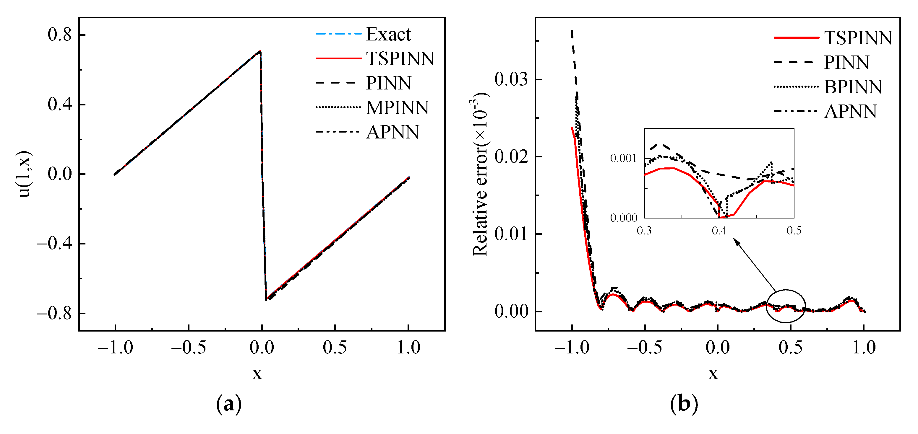
  • Example 3 (1D viscous Burgers’ equation):
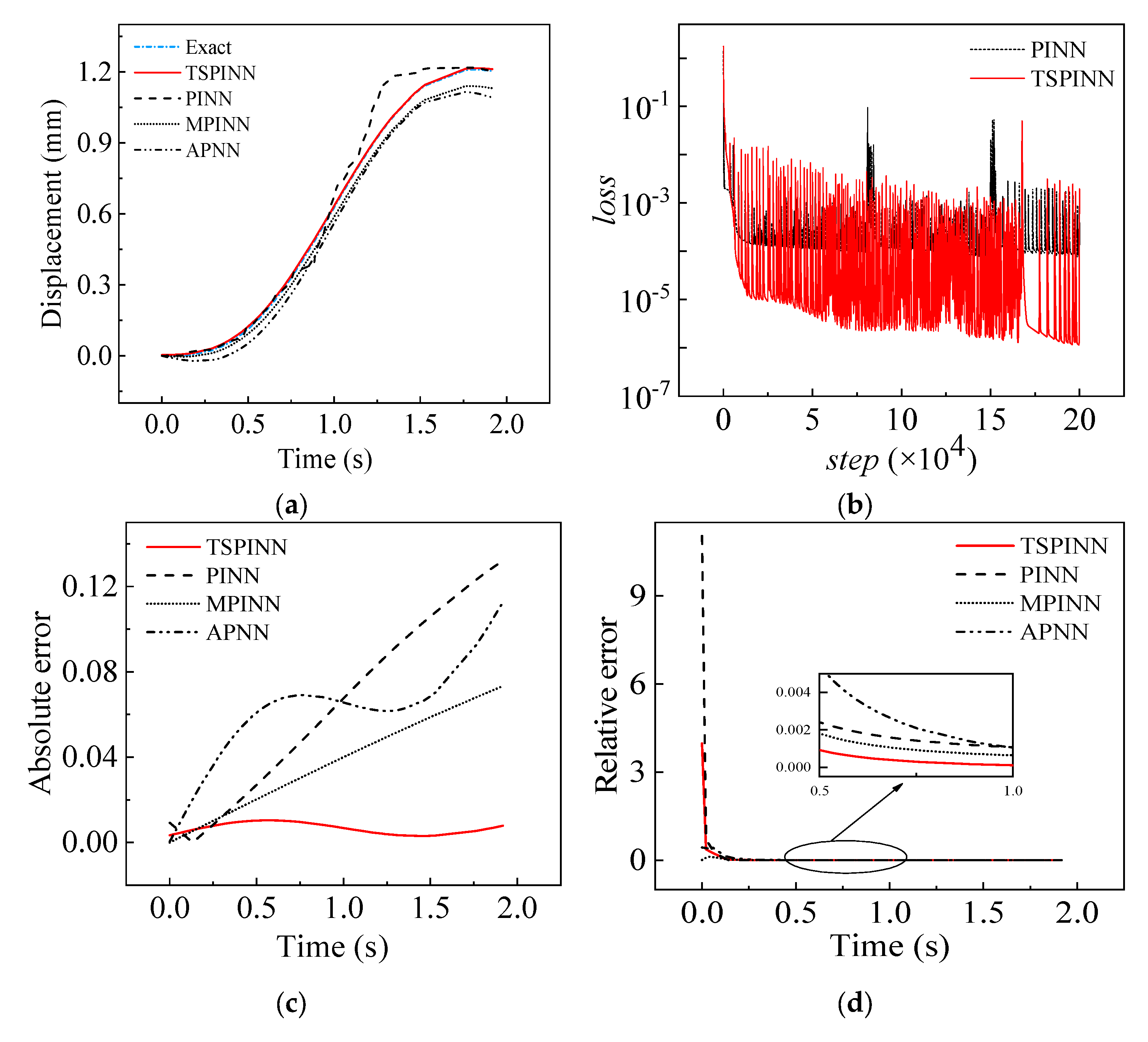
t u + u u x ε u x x = 0
with initial conditions of
u 0 , x = s i n ( π ( x x 0 ) )
and boundary conditions of
u t , 1 = u t , 1 = g ( t )
where g ( t ) is determined from the exact solution:
u x , t = 2 ε x v v , v = e x p ( c o s ( π ( x x 0 2 ε t s ) ) 2 π ε ) e s 2 d s
The TSPINNs that enforces the Dirichlet boundary condition, x 2 1 N x , ε λ x x c , ε λ + g ( t ) , was employed to solve the Burger’s equation under a small viscosity parameter ε .
While ε = 10 3 π , for x 0 = 0 , the inner layer (nearly a shock profile) is located at the center of the domain. According to (11), x 0 = 0 leads to g ( t ) = 0 . When t = 1 , the numerical results in Figure 4. From Figure 4b, the maximal relative error at the final time t = 1 is 2.4%.
  • Example 4 (SDOF):
m u ¨ + k u = 2 s i n ω t , ε = m / k , ω = 3.14 ,   0 < t < 2
In the dynamic response analysis of SDOF structures with ε = 10, as shown in Figure 5, TSPINN predictions exhibit closer agreement with numerical solutions in comparative analysis with other PINN variants, achieving near 85% error reduction. Furthermore, TSPINN demonstrates faster loss convergence, requiring 40% less training time: its loss value reaches 10−6 magnitude, whereas conventional PINN stagnates at 10−3. This comparison demonstrates TSPINN’s dual enhancement in prediction accuracy and training efficiency for rigid modal coupling scenarios.
At ε = 10−2, as shown in Figure 6, TSPINN’s predictions demonstrate strong agreement with numerical solutions, with both absolute and relative error being significantly reduced compared to conventional PINN and its variants. The loss function of TSPINN converges to 10−7, whereas traditional PINN compared to converges at 10−5.
At ε = 10−3, as shown in Figure 7, the predictions of TSPINN are in good agreement with the numerical solutions. The loss function converges to 10−5, representing two orders of magnitude improvement over traditional PINNs (10−3). In this scenario, TSPINN exhibits superior performance: the maximum absolute error of the PINN variants reaches 1.2 × 10⁻⁴, whereas TSPINN maintains an error of only 1 × 10⁻⁵. Although the final convergence value is slightly higher than previous cases (ε = 10 and 10−2), stable convergence efficiency persists, demonstrating the model’s robustness in small parameter regimes.
In summary, traditional PINNs demonstrate numerical pathologies of stiff systems as ε 0 , including oscillatory divergence in derivatives and high-frequency component loss. TSPINNs maintain equilibrium between solution accuracy and numerical stability in large gradient regions through their ε-embedded scale-aware mechanism, exhibiting lower derivative reconstruction error than conventional methods. These results demonstrate the theoretical advantages of the proposed method for rigid modal coupling dynamics.

3. Parameter Inversion

To validate the engineering applicability of TSPINNs for structural dynamic parameter inversion, multi-condition vibration tests were conducted on T-shaped tower structures. Firstly, experimentally measured displacement responses were quantitatively compared with the model predictions to verify the forward modeling precision. Secondly, a parameter inversion framework based on data and physics information was established, and the reliability of TSPINNs was evaluated by the relative error between the inversion results and the theoretical values based on the predefined damage parameters.

3.1. Finite Elements Error

In the theoretical basis of the TSPINNs, the finite elements are assumed to be calibrated with no modeling error. However, finite elements error is inevitable in practice. Therefore, the influence of the finite elements error is investigated here.
Three cases were adopted to simulate finite elements errors. The structural parameters are detailed in Table 2, and a sinusoidal excitation was applied to the midpoint of the tower column; the results of each following condition are shown in Figure 5.
As shown in Figure 8, the number of elements used in the finite element model has a significant impact on the accuracy of the calculation results. Therefore, during the numerical computation of structural response, the finite element method (FEM) was divided into 20 beam elements, resulting in 21 nodes and 60 degrees of freedom. To simplify the computation process, only the planar deformation of the structure is considered during the calculations, and the effect of damping on the structural response is neglected.

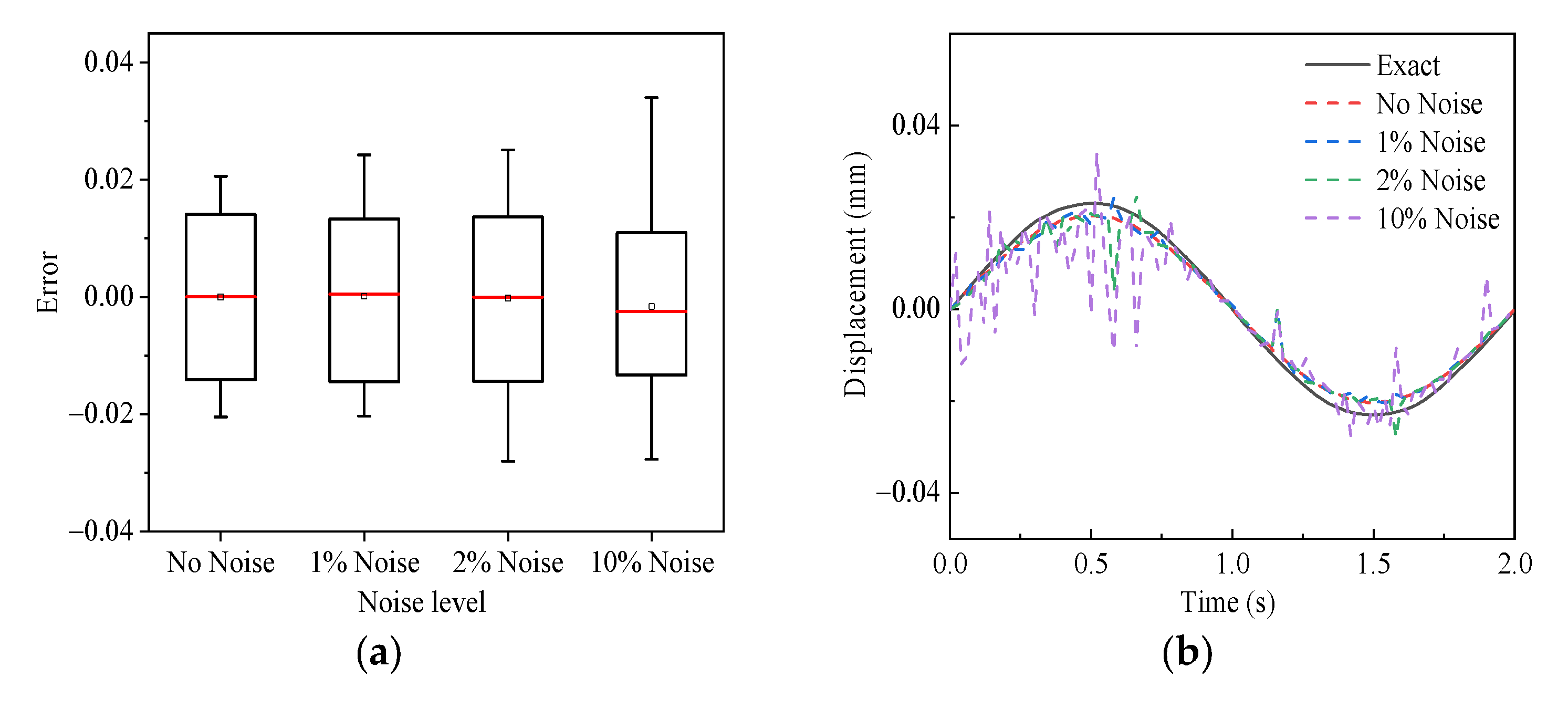
3.2. Observation Noise
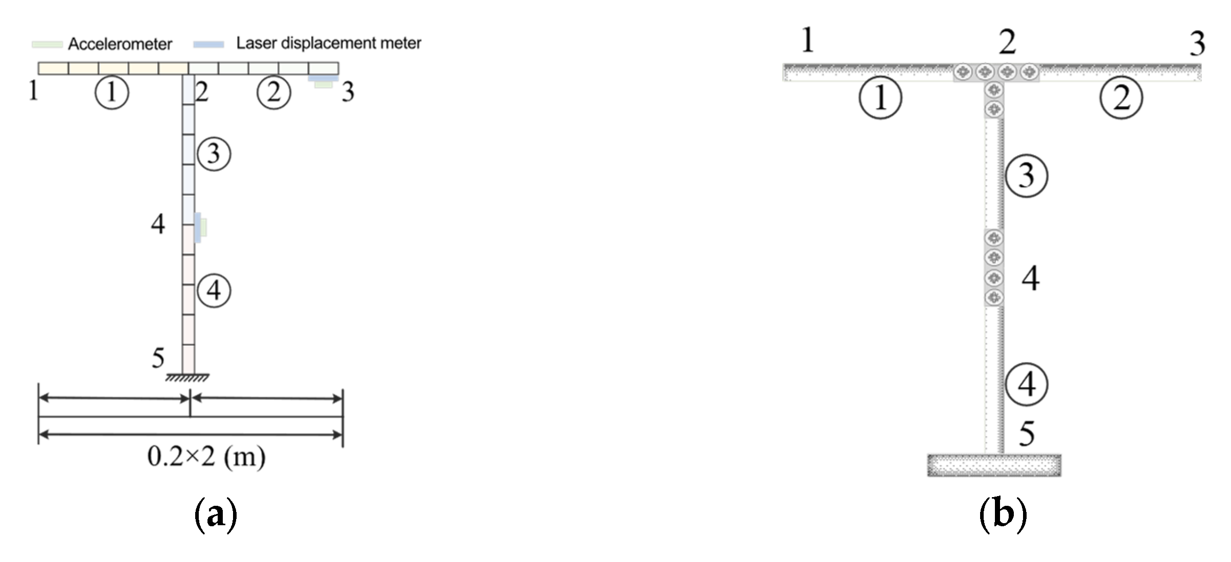
To verify the noise robustness of TSPINNs, Gaussian white noise levels of 1%, 2%, and 10% were added to the structural displacement response solutions (with the noise ratio defined as the ratio of the noise standard deviation to the response standard deviation). The MSPE of TSPINNs’ predicted results is shown in Figure 9. As the noise intensity increases, the recognition error range of TSPINNs tends to expand, and the dispersion of the prediction results also increases, indicating that the model still maintains basic robustness under conventional noise conditions; however, its performance exhibits a significant degradation trend in high-intensity noise scenarios.
M S P E = 100 N % i = 1 N y i y ^ i y i

3.3. Problem Setup

The T-shaped tower structure, a simplified model of transmission towers, is crucial for power transmission as a key supporting system. This paper employs the T-shaped structure to verify the TSPINNs method. Given that the algorithm for complex structures is the same as for simplified ones, the simple structure’s algorithm can be extended to complex cases. Thus, the T-shaped structure is chosen for computational validation.
In the finite element analysis framework, each beam element is discretized into five finite element segments, yielding a total of 20 elements. Structural damage is uniformly conceptualized as member damage, mechanically simulated through cross-sectional area modification of corresponding members. This study strategically adopts TSPINNs to inversely identify critical parameters including mass and stiffness distributions in damaged configurations. The structural geometry and element numbering distribution are visualized in Figure 9.
Calculate the stiffness matrix and mass matrix of the element in the global coordinate system using the stiffness matrix and mass matrix in the standard local coordinate system of the element.
K e = E A / L 0 0 0 12 E I / L 3 6 E I / L 2 0 6 E I / L 2 4 E I / L E A / L 0 0 0 12 E I / L 3 6 E I / L 2 0 6 E I / L 2 2 E I / L E A / L 0 0 0 12 E I / L 3 6 E I / L 2 0 6 E I / L 2 2 E I / L E A / L 0 0 0 12 E I / L 3 6 E I / L 2 0 6 E I / L 2 4 E I / L
M e = ρ A L 420 140 0 0 70 0 0 0 156 22 L 0 54 13 L 0 22 L 4 L 2 0 13 L 3 L 2 70 0 0 140 0 0 0 54 13 L 2 0 156 22 L 0 13 L 3 L 2 0 22 L 4 L 2
The element stiffness matrix and the element mass matrix in the local coordinate system need to be transformed into the global coordinate system form using Formula (16):
K ¯ e = T T K e T M ¯ e = T T M e T
T = c o s α s i n α 0 0 0 0 s i n α c o s α 0 0 0 0 0 0 1 0 0 0 0 0 0 c o s α s i n α 0 0 0 0 s i n α c o s α 0 0 0 0 0 0 1
α is the angle between the x-axis of the planar frame element coordinate system and the positive direction of the x-axis of the overall coordinate system, measured counterclockwise, and T T is the transpose of the transformation matrix.
The finite element model of the T-shaped tower structure was developed using MATLAB R2018a, with the global stiffness matrix K and mass matrix M systematically assembled through direct stiffness method implementation. The governing dynamic equilibrium equation is formulated as
M u ¨ t + C u ˙ t + K u ( t ) = P s i n ω t
u ¨ t = [ u ¨ 1 , u ¨ 2 , , u ¨ 62 , u ¨ 63 ] T
u ˙ t = [ u ˙ 1 , u ˙ 2 , , u ˙ 62 , u ˙ 63 ] T
u t = [ u 1 , u 2 , , u 62 , u 63 ] T
where M denotes the mass matrix, C the damping matrix, K the stiffness matrix, ü(t) the nodal acceleration vector, u(t) the displacement vector, and P s i n ω t the harmonic excitation force vector. Initial conditions are specified as
u 0 = 0 , u ¨ 0 = 0

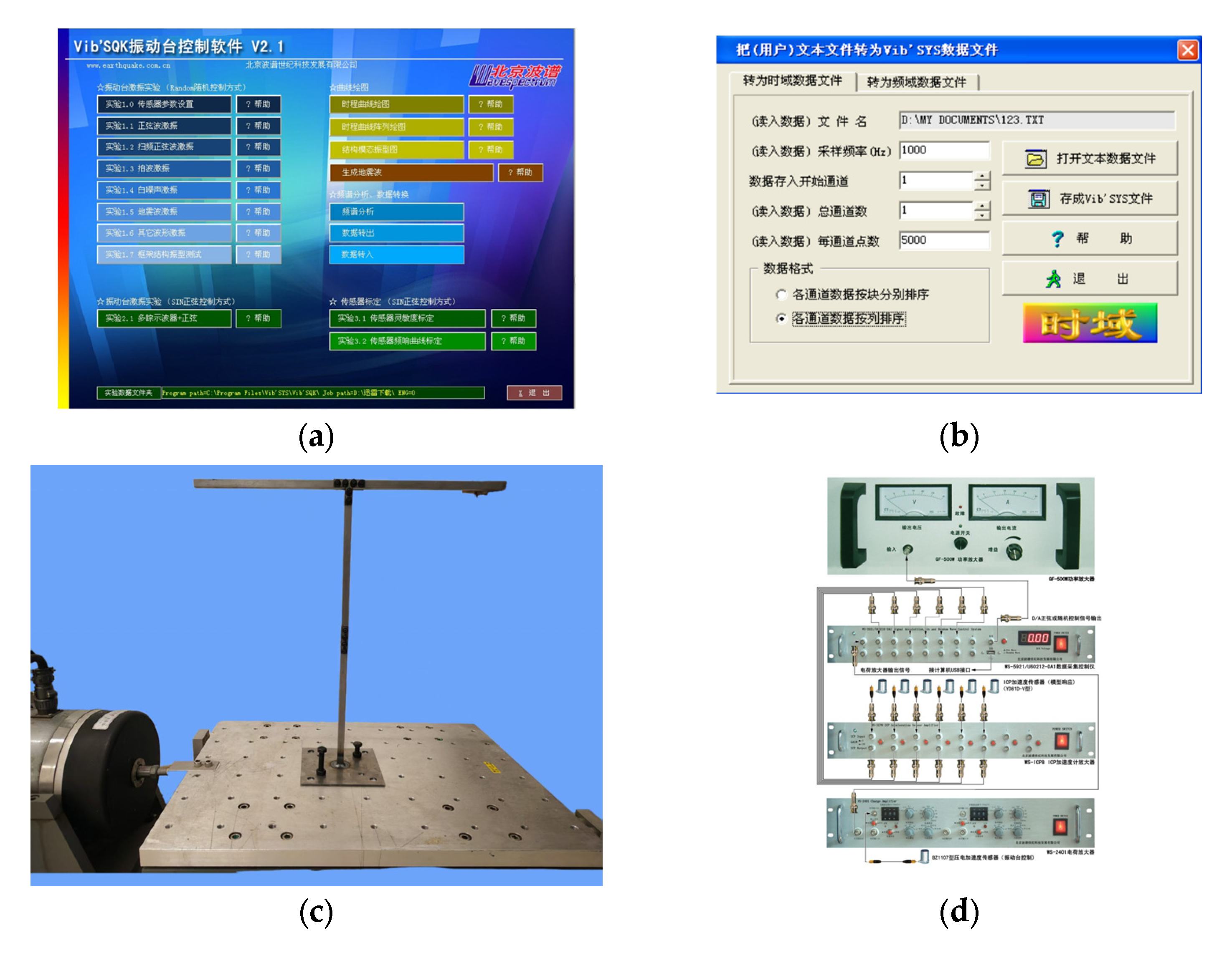
3.4. Experiment Setup

Numerical simulations were conducted for a prototype structure with characteristic pole length of L = 0.2 m, as shown in Figure 10. The complete set of geometric and material parameters is cataloged in Table 3.
As shown in Figure 11, a shaking table was used to simulate multiple types of vibration excitations. The Vib’SQK control system precisely regulates vibration frequency, amplitude, and phase parameters to replicate structural dynamic responses of the tower. The operational workflow comprises three stages:
(1)
The programmable signal generation produces excitation signals.
(2)
Power amplification actuates the electrodynamic shaker.
(3)
Closed-loop feedback enables real-time parameter adjustment while synchronously acquiring response data.
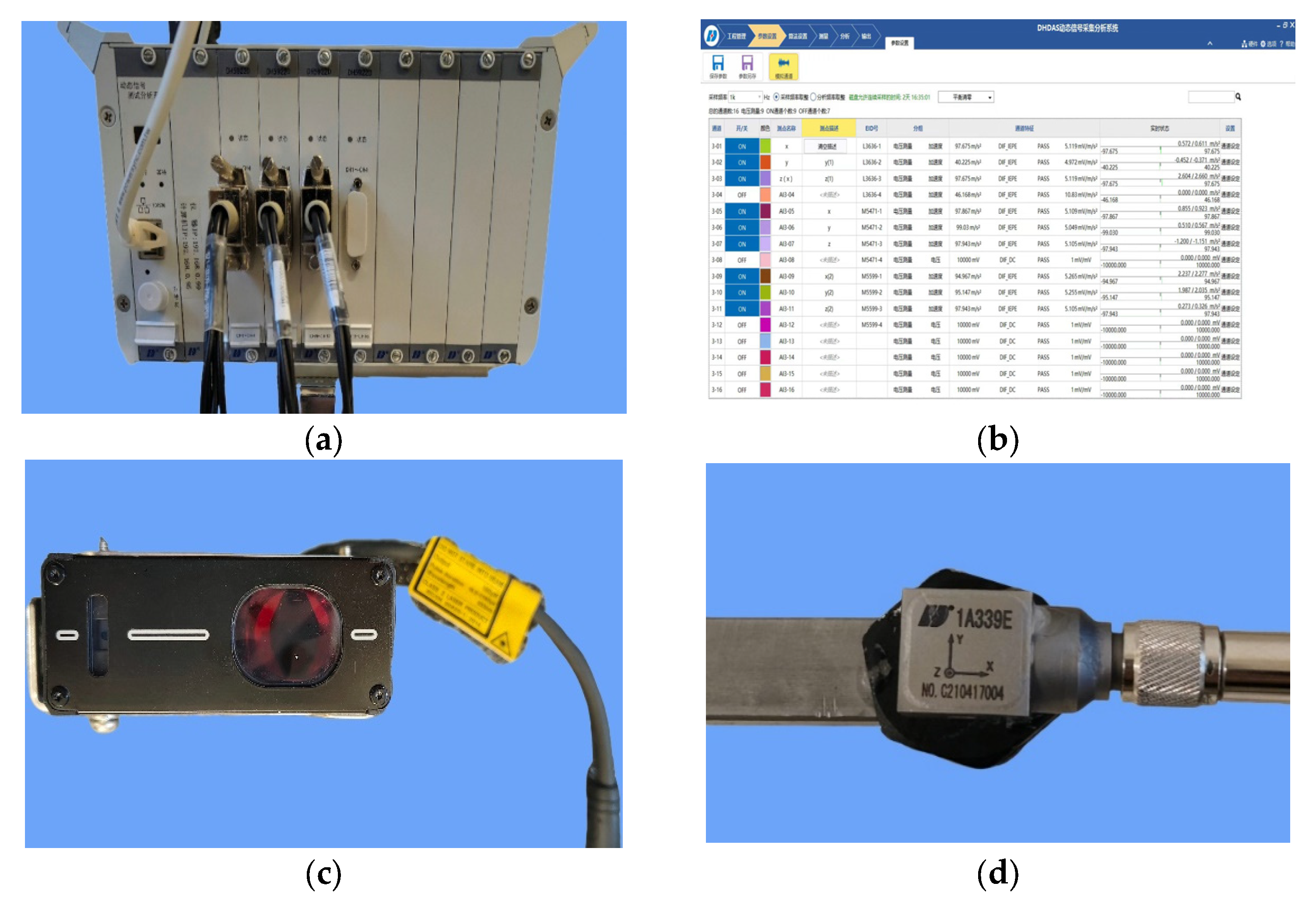
The data acquisition system comprises three parts (Figure 12).
(1)
DH5922D dynamic signal analysis system: Provides 256 kHz/channel synchronous sampling, incorporating signal conditioning and anti-aliasing filter for parallel acquisition of multi-physical signals.
(2)
Keyence laser displacement sensor (LK—H151): Captures spot displacement via laser triangulation with micron-level resolution.
(3)
Donghua test accelerometer (1A339E): Utilizes a mass-spring-piezoelectric sensing system with a linearity error of ≤±1%FS.

3.5. Test Condition

When there is a significant disparity in the norms between the mass matrix (M), stiffness matrix (K), and damping matrix (C) (e.g., K M , ε = M / K 1 ), it results in the occurrence of high-frequency oscillations and boundary layer effects. To address this issue, the TSPINNs method introduced in Section 2.1 is employed to solve structural responses and conduct parameter identification after damage.
As shown in Table 4, the operational conditions are categorized based on damage severity levels of structural members, establishing distinct operational scenarios for analysis. The structural loading is defined as harmonic loading 2000 s i n ( ω t ) N .

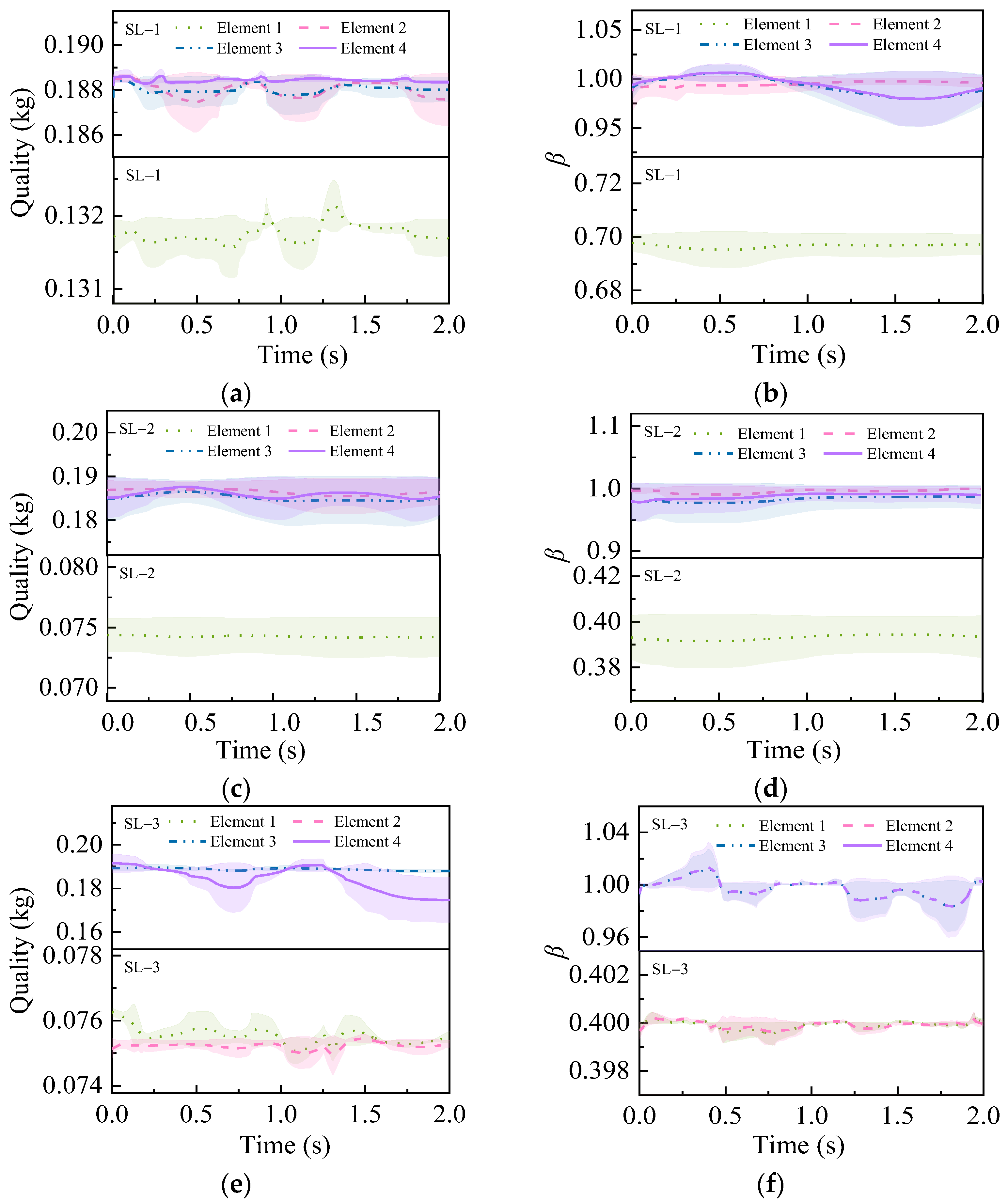
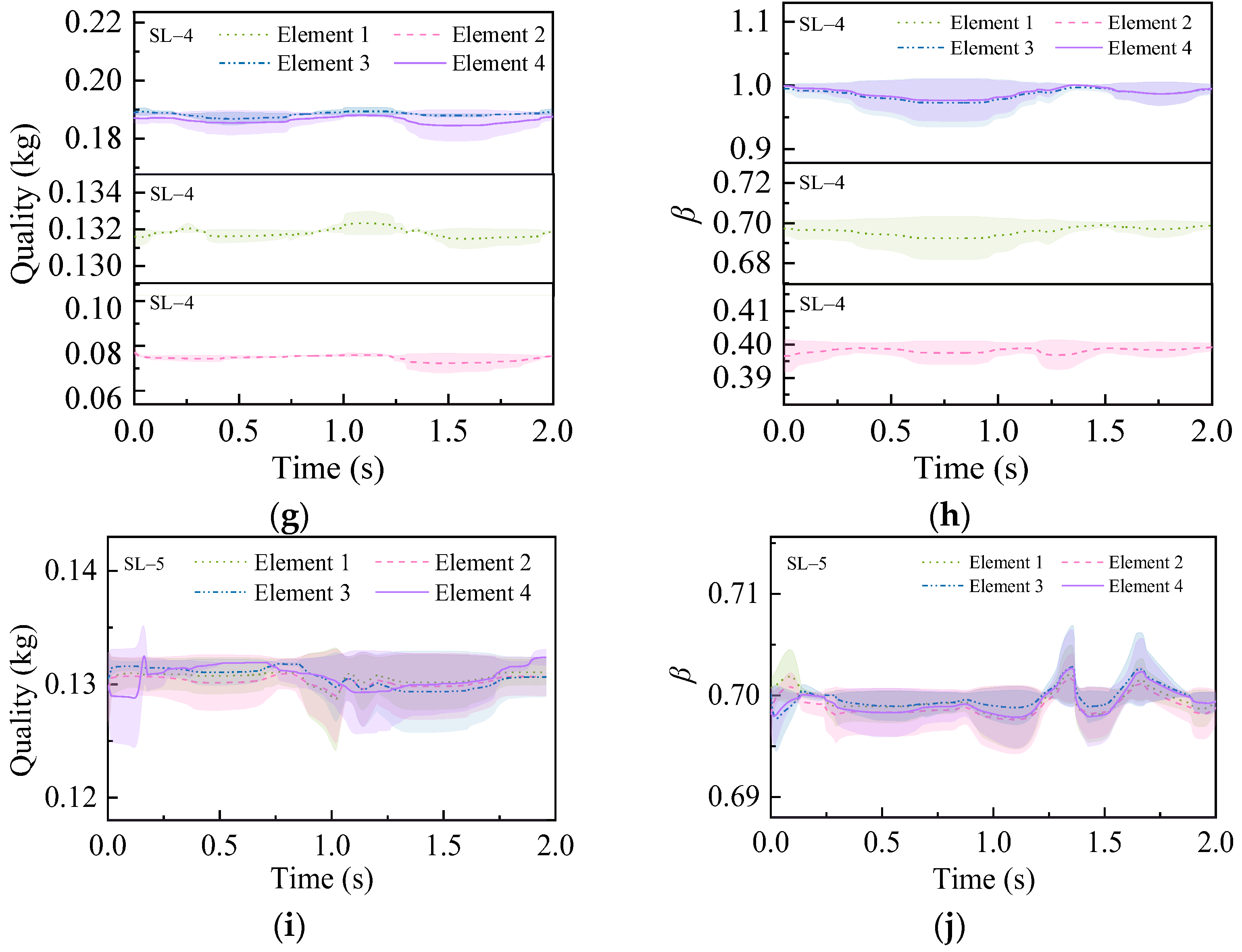
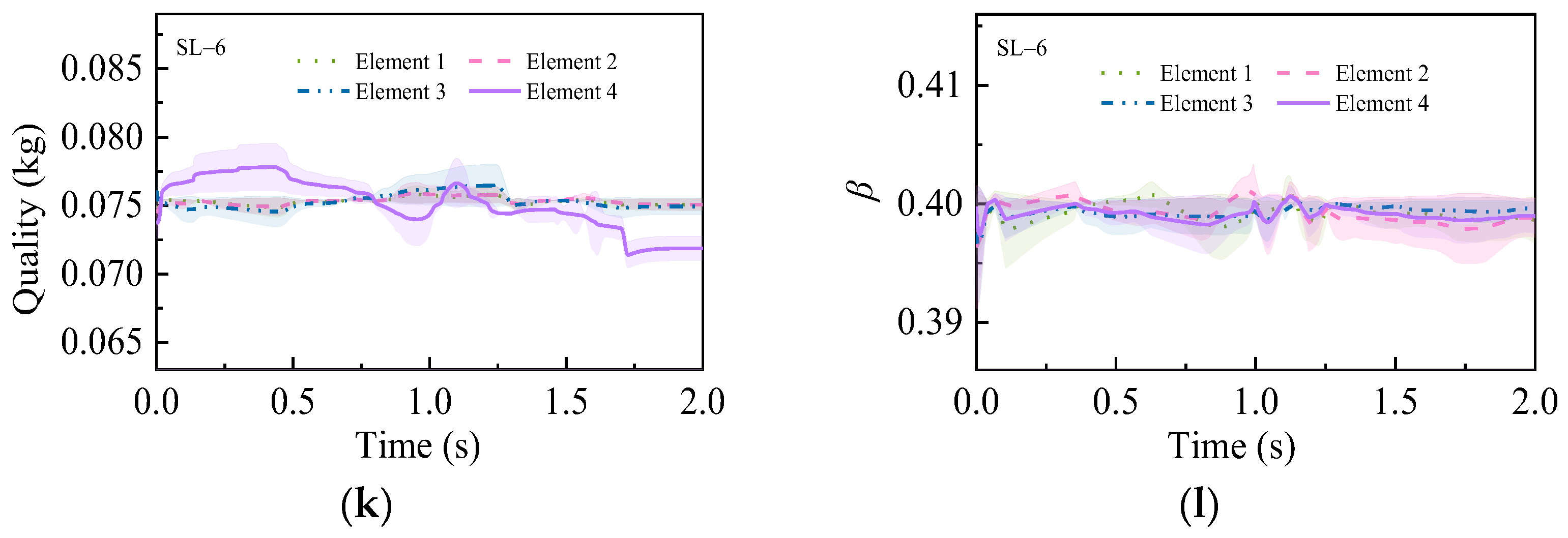
3.6. T-Shaped Tower Structure Structural Parameters Inversion

Taking the simplified T-shaped tower structure as the research object, the network architecture of TSPINNs is shown in Figure 13. The network input layer is composed of t , ε λ t f i n a l t c , ε λ , while the hidden layer applies nonlinear transformations through neural network NN (w, b) with the Tanh activation function. The output layer of the network is adaptively configured based on the problem type: predicting displacement u in forward modeling or simultaneously outputting u and parameters coefficient β in inverse problems.
The loss function combines and the positive problem integrates the initial conditions initial/boundary conditions and PDE residuals for forward problems. Inverse problems additionally incorporate data discrepancies between experimental and predicted values. Parameter optimization via gradient descent continues until the total loss reaches convergence threshold.
In structural parameter identification, intrinsic properties such as mass, stiffness, and damping exhibit dynamic evolution. The stiffness reduction coefficient ( β = K d a m a g e d / K i n t a c t ) as the primary identification metric to quantify structural damage severity. Let β i , i = 1 , , 4 denote stiffness reduction factors for elements 1–4. The comparative analysis of TSPINN-predicted β values enables precise damage localization and severity quantification. For instance, β 1 = 0.9 with   β 2 ~ β 4 = 1 , indicates 10% stiffness loss in Element 1.
To demonstrate the effectiveness and robustness of the TSPINNs algorithm, structural parameters were analyzed based on the experimental data with damage states defined in Table 2. For forward problem validation, SL-1 and SL-2 cases were analyzed.
Figure 14 presents the TSPINN’s performance in SL-1 and SL-2 cases. The predictions of node 1 and 4 demonstrate strong agreement with the experimental values (SL-1 standard deviations: 2.66 × 10⁻⁵–3.58 × 10⁻² for node 1; 4.81 × 10⁻⁷–1.21 × 10⁻² for node 4), revealing that the prediction of tower column midpoint exhibits superior accuracy of the midpoint of the tower column is higher. End-time domain prediction deviations in SL-1 likely stem from stiffness degradation-induced nonlinearities during late vibration phases. Nevertheless, the overall error is still within a controllable range, confirming that TSPINNs effectively capture structural response modes while maintaining stability under nonlinear disturbances.
SL-2 shows increased deviations compared to SL-1 (standard deviations: 4.73 × 10⁻⁵–5.66 × 10⁻² for node 1; 1.25 × 10⁻⁵–2.29 × 10⁻² for node 4). Although the error band widens marginally, the temporal error distribution remains relatively stable, demonstrating that TSPINNs retain reliable learning capability post-severe structural damage.
Figure 15 compares the identification results of TSPINNs with ground true values across operational cases SL-1 to SL-6. Results demonstrate that TSPINNs achieve high identification accuracy for structural stiffness reduction coefficients and mass parameters, with maximum errors controlled within 10% across all cases. Detail analysis reveals the following:
(1)
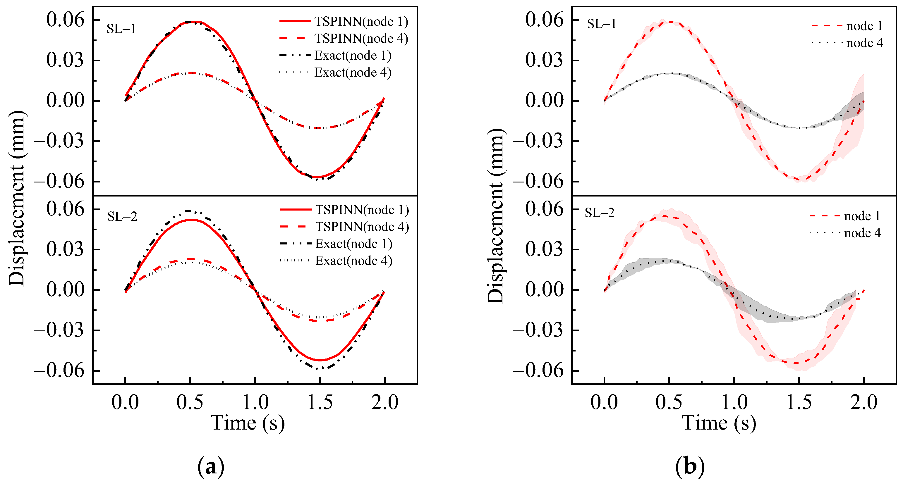
Compared to element 1 and element 2, elements 3 and 4 exhibit slightly increased identification deviations, though remaining within acceptable engineering tolerance ranges.
(2)
With the increase in structural damage severity (SL-1 to SL-2), TSPINNs show more stable identification ability, yielding narrower error bandwidths.
(3)
When comparing structural cases with varying damage severities (SL-3 vs. SL-4) at identical positions, TSPINNs show greater confidence in mass parameter identification for cross-damage-level comparisons than for same-severity cases, with significantly tighter error distributions substantiating this enhanced reliability.
(4)
When all elements are damaged simultaneously (SL-5 to SL-6), TSPINNs maintain a robust performance (peak standard deviation ≤ 1.09 × 10⁻²).
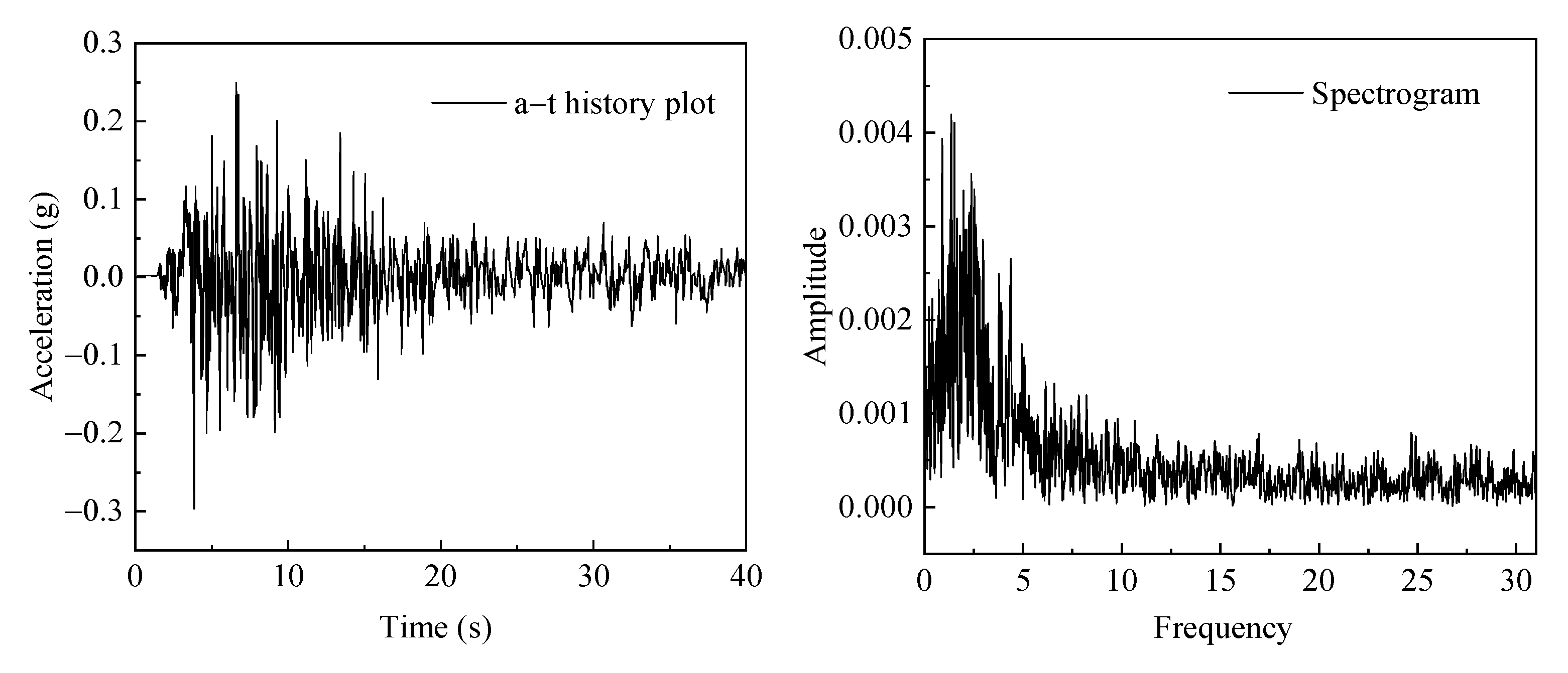
Under random load excitation (Figure 16), the identification performance of TSPINNs was evaluated for SL-7 and SL-8. Figure 17 comparisons reveal the following:
(1)
Load identification errors surge in the 5–10 s interval (peaking at 17%), potentially attributed to nonlinear response abruptions;
(2)
Higher inversion accuracy (mean error < 3%) prevails in other periods.
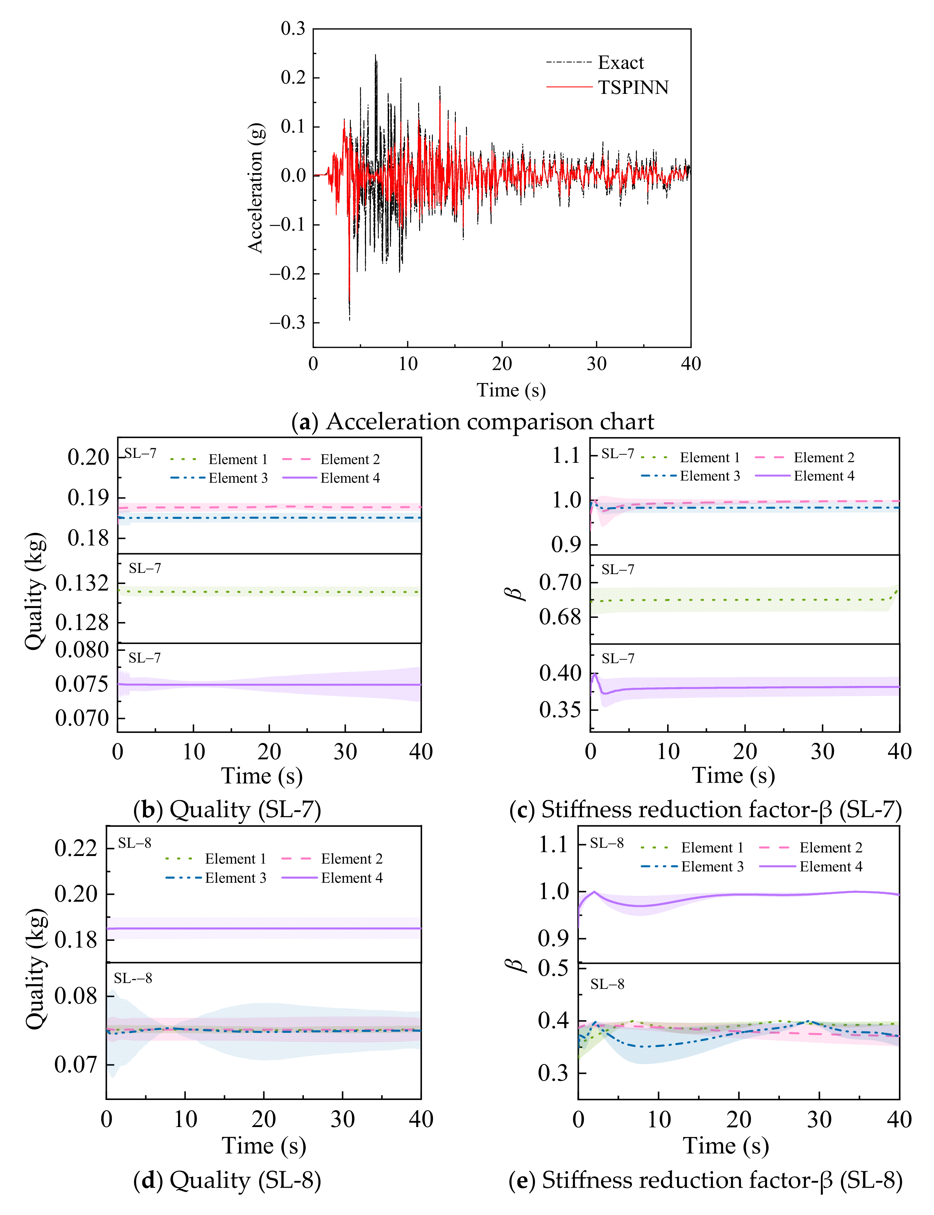
For both SL-7 and SL-8:
(1)
Stiffness reduction coefficient identification achieves a 2.7% mean error;
(2)
Mass parameters identification maintains a 0.46% mean error;
(3)
Error bandwidth fluctuation remains <2%.
These results confirm that TSPINNs deliver accurate and stable identification under stochastic loading conditions.

4. Conclusions

To address safety assessment challenges for T-shaped tower structures prevalent in civil engineering, this study proposes two-scale physics-informed neural networks (TSPINNs), validating its efficacy through theoretical analysis and experimental verification. The main conclusions are as follows:
(1)
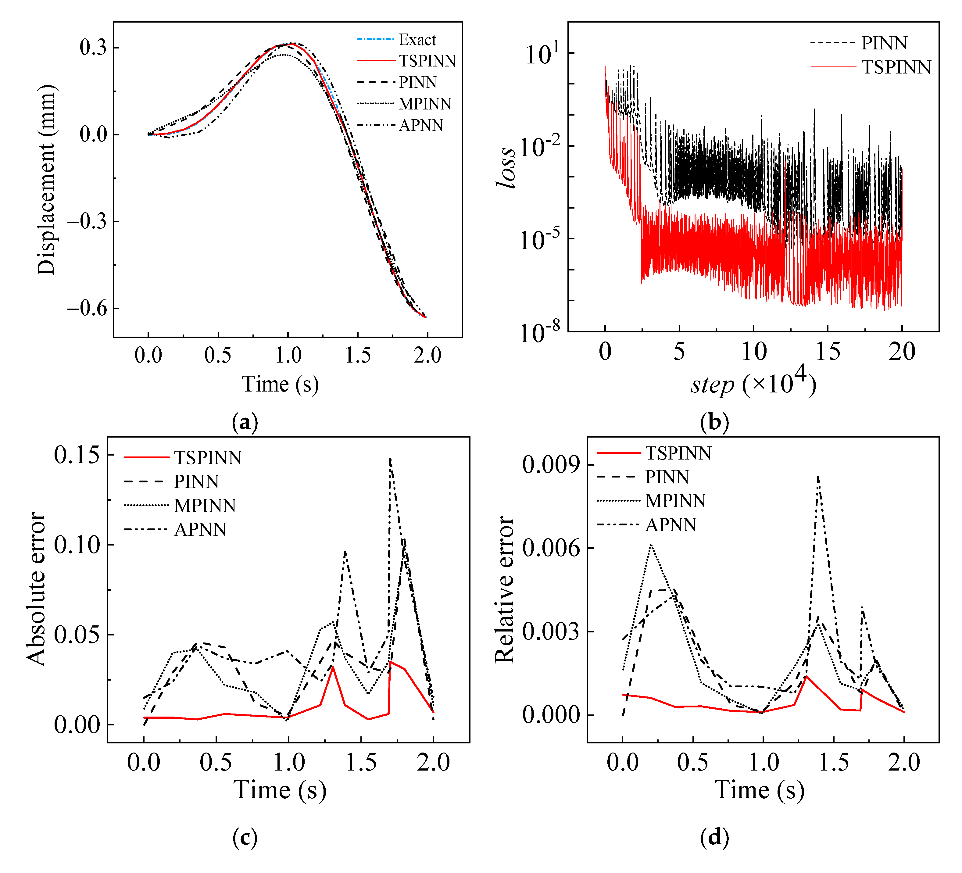
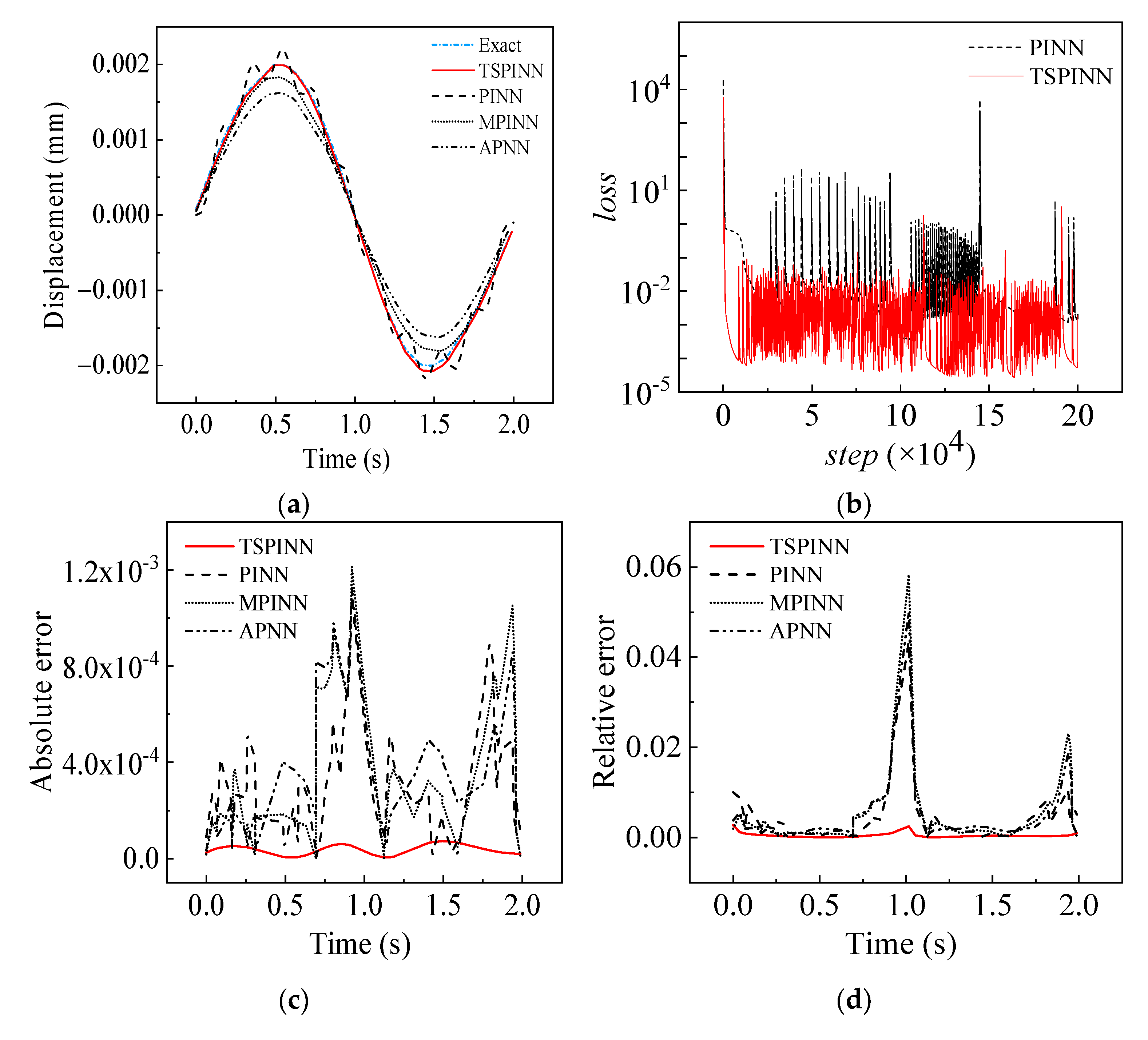
Dynamic response analysis of SDOF demonstrates TSPINNs’ technical superiority in stiff modal coupling scenarios:
  • One to two orders of magnitude improvement in prediction accuracy over conventional PINNs;
  • Accelerated loss function convergence with 2–3 orders of magnitude lower final residuals;
  • Effective mitigation of numerical oscillations in high-gradient regions via ε-parameter scale-aware mechanisms.
(2)
Shaking table test on a T-tower prototype establishes a damage scenario database, revealing the following:
  • Less than 10% average maximum deviation between identified and experimental mass/stiffness parameters;
  • Robust performance under complex damage scenarios.
These results resolve critical limitations in conventional structural health monitoring (SHM), including data acquisition challenges and insufficient identification accuracy. TSPINNs’ multi-scale feature fusion mechanism delivers a theoretical innovation and engineering-feasible solution for the intelligent diagnosis of complex engineering structures.
The proposed method is limited in the following aspects.
(1)
Computational cost: The TSPINN method may incur high computational costs when addressing more complex problems, requiring advanced hardware configurations. Future work should focus on algorithm optimization to reduce computational resource demands and improve efficiency, thereby enhancing the method’s feasibility across diverse computational environments.
(2)
Sensitivity to network hyperparameters: Like many machine learning methods, TSPINNs’ performance is sensitive to hyperparameter selection (e.g., learning rate, network depth, neuron count per layer). Inappropriate hyperparameters may lead to slow training, convergence difficulties, or overfitting, compromising accuracy and generalizability. Future efforts should prioritize systematic hyperparameter tuning strategies to minimize manual intervention and improve model stability and reliability.
(3)
Scalability: The current validation is limited to simplified structures (such as T-shaped towers). More complex geometries (irregular trusses, multi-physical field coupling) require the integration of modular sub-networks or domain decomposition techniques.
(4)
Noise Robustness: Robustness and accuracy are relatively good under low noise conditions; however, performance is significantly affected in high noise scenarios, leading to reduced reliability. It is necessary to integrate denoising (wavelet transforms) and uncertainty quantification (Bayesian framework).
(5)
The capability of the proposed methodology to characterize complex structural parameters under minor damage conditions remains unverified. Given that minor structural degradation necessitates quantitative characterization for establishing TSPINNs’ damage identification viability, subsequent investigations will prioritize the development of systematic quantification frameworks and algorithm robustness enhancement.

Author Contributions

Conceptualization, Y.Z.; Methodology, X.L.; Formal analysis, X.Z.; Investigation, Z.Y.; Writing—review & editing, Y.H. All authors have read and agreed to the published version of the manuscript.

Funding

This research was funded by the China Postdoctoral Science Foundation grant number 2023M734083, the Chongqing Key Laboratory of Disaster Prevention and Reduction in Power Transmission Engineering research project grant number EEMDPM2021207, and the Chongqing University of Science and Technology scientific research project grant number KJDX2024008. The APC was funded by Chongqing University of Science and Technology scientific research project grant number KJDX2024008.

Data Availability Statement

The original contributions presented in this study are included in the article. Further inquiries can be directed to the corresponding authors.

Conflicts of Interest

The authors declare no conflict of interest.

References

  1. Yuen, K.V.; Au, S.K.; Beck, J. Two-Stage structural health monitoring approach for Phase I benchmark studies. J. Eng. Mech. 2004, 130, 16–33. [Google Scholar] [CrossRef]
  2. Yin, T.; Jiang, Q.H.; Yuen, K.V. Vibration-based damage detection for structural connections using incomplete modal data by Bayesian approach and model reduction technique. Eng. Struct. 2017, 132, 260–277. [Google Scholar] [CrossRef]
  3. Lai, Z.; Nagarajaiah, S. Sparse structural system identification method for nonlinear dynamic systems with hysteresis/inelastic behavior. Mech. Syst. Signal Process. 2019, 117, 813–842. [Google Scholar] [CrossRef]
  4. Banerjee, B.; Roy, D.; Vasu, R.M. Self-regularized pseudo time-marching schemes for structural system identification with static measurements: Self-regularized pseudo time-marching schemes. Int. J. Numer. Methods Eng. 2010, 82, 896–916. [Google Scholar] [CrossRef]
  5. Pathirage, C.S.N.; Li, J.; Li, L.; Hao, H.; Liu, W.; Ni, P. Structural damage identification based on autoencoder neural networks and deep learning. Eng. Struct. 2018, 172, 13–28. [Google Scholar] [CrossRef]
  6. Guo, F.; Cui, Q.; Zhang, H.; Wang, Y.; Zhang, H.; Zhu, X.; Chen, J. A new deep learning-based approach for concrete crack identification and damage assessment. Adv. Struct. Eng. 2024, 27, 2303–2318. [Google Scholar] [CrossRef]
  7. Hu, S.L.J.; Yang, W.L.; Li, H.J. Signal decomposition and reconstruction using complex exponential models. Mech. Syst. Signal Process. 2013, 40, 421–438. [Google Scholar]
  8. Bao, N.; Zhang, T.; Huang, R.; Biswal, S.; Su, J.; Wang, Y. A Deep Transfer Learning Network for Structural Condition Identification with Limited Real-World Training Data. Struct. Control Health Monit. 2023, 2023, 18. [Google Scholar] [CrossRef]
  9. He, Z.C.; Zhang, Z.; Li, E. Multi-source random excitation identification for stochastic structures based on matrix perturbation and modified regularization method. Mech. Syst. Signal Process. 2019, 119, 266–292. [Google Scholar] [CrossRef]
  10. Shu, J.; Ding, W.; Zhang, J.; Lin, F.; Duan, Y. Continual-learning-based framework for structural damage recognition. Struct. Control Health Monit. 2022, 29. [Google Scholar] [CrossRef]
  11. Lu, L.; Jin, P.; Pang, G.; Zhang, Z.; Karniadakis, G.E. Learning nonlinear operators via DeepONet based on the universal approximation theorem of operators. Nat. Mach. Intell. 2021, 3, 218–229. [Google Scholar] [CrossRef]
  12. Li, Z.; Kovachki, N.; Azizzadenesheli, K.; Liu, B.; Bhattacharya, K.; Stuart, A.; Anandkumar, A. Fourier Neural Operator for Parametric Partial Differential Equations. In Proceedings of the International Conference on Learning Representations, Vienna, Austria, 3–7 May 2021. [Google Scholar]
  13. Xu, C.; Cao, B.T.; Yuan, Y.; Meschke, G. Transfer learning based physics-informed neural networks for solving inverse problems in engineering structures under different loading scenarios. Comput. Methods Appl. Mech. Eng. 2023, 405, 115852. [Google Scholar] [CrossRef]
  14. Penwarden, M.; Zhe, S.; Narayan, A.; Kirby, R.M. A metalearning approach for Physics-Informed Neural Networks (PINNs): Application to parameterized PDEs. J. Comput. Phys. 2023, 477, 111912. [Google Scholar] [CrossRef]
  15. Shi, W.; Huang, X.; Gao, X.; Wei, X.; Zhang, J.; Bian, J.; Yang, M.; Liu, T.-Y. LordNet: Learning to Solve Parametric Partial Differential Equations without Simulated Data. arXiv 2022, arXiv:2206.09418. [Google Scholar]
  16. Koric, S.; Abueidda, D.W. Data-driven and physics-informed deep learning operators for solution of heat conduction equation with parametric heat source. Int. J. Heat Mass Transf. 2022, 203, 123809. [Google Scholar] [CrossRef]
  17. Wang, S.; Perdikaris, P. Long-time integration of parametric evolution equations with physics-informed DeepONets. J. Comput. Phys. 2022, 475, 111855. [Google Scholar] [CrossRef]
  18. Raissi, M.; Perdikaris, P.; Karniadakis, G.E. Physics-Informed Neural Networks: A Deep Learning Framework for Solving Forward and Inverse Problems Involving Nonlinear Partial Differential Equations. J. Comput. Phys. 2019, 378, 686–707. [Google Scholar] [CrossRef]
  19. Raissi, M.; Perdikaris, P.; Karniadakis, G.E. Physics Informed Deep Learning (Part II): Data-driven Discovery of Nonlinear Partial Differential Equations. arXiv 2017, arXiv:1711.10566. [Google Scholar]
  20. Lu, L.; Meng, X.; Mao, Z.; Karniadakis, G.E. DeepXDE: A deep learning library for solving differential equations. SIAM Rev. 2021, 63, 208–228. [Google Scholar] [CrossRef]
  21. Nabian, M.A.; Meidani, H. A Deep Neural Network Surrogate for High-Dimensional Random Partial Differential Equations. arXiv 2018, arXiv:1806.02957. [Google Scholar]
  22. Zhang, D.; Guo, L.; Karniadakis, G.E. Learning in Modal Space: Solving Time-Dependent Stochastic PDEs Using Physics-Informed Neural Networks. SIAM J. Sci. Comput. 2020, 42, A639–A665. [Google Scholar] [CrossRef]
  23. Zhang, D.; Lu, L.; Guo, L.; Karniadakis, G.E. Quantifying total uncertainty in physics-informed neural networks for solving forward and inverse stochastic problems. J. Comput. Phys. 2019, 397, 108850. [Google Scholar] [CrossRef]
  24. Rahaman, N.; Arpit, D.; Baratin, A.; Draxler, F.; Lin, M.; Hamprecht, F.A.; Bengio, Y.; Courville, A. On the Spectral Bias of Deep Neural Networks. arXiv 2018, arXiv:1806.08734. [Google Scholar]
  25. Basri, R.; Jacobs, D.; Kasten, Y.; Kritchman, S. The Convergence Rate of Neural Networks for Learned Functions of Different Frequencies. arXiv 2019, arXiv:1906.00425. [Google Scholar]
  26. Zhang, T.; Dey, B.; Kakkar, P.; Dasgupta, A.; Chakraborty, A. Frequency-compensated PINNs for Fluid-dynamic Design Problems. arXiv 2020, arXiv:2011.01456. [Google Scholar]
  27. Baydin, A.G.; Pearlmutter, B.A.; Radul, A.A.; Siskind, J.M. Automatic differentiation in machine learning: A survey. J. Mach. Learn. Res. 2018, 18, 1–43. [Google Scholar]
  28. Wang, N.; Chen, Q.; Chen, Z. Reconstruction of nearshore wave fields based on physics-informed neural networks. Coast. Eng. 2022, 176, 104167. [Google Scholar] [CrossRef]
  29. Jeong, H.; Bai, J.; Batuwatta-Gamage, C.; Rathnayaka, C.; Zhou, Y.; Gu, Y. A Physics-Informed Neural Network-based Topology Optimization (PINNTO) framework for structural optimization. Eng. Struct. 2022, 278, 115484. [Google Scholar] [CrossRef]
  30. Luong, K.A.; Le-Duc, T.; Lee, J. Deep reduced-order least-square method—A parallel neural network structure for solving beam problems. Thin-Walled Struct. 2023, 191, 111044. [Google Scholar] [CrossRef]
  31. Niu, J.; Xu, W.; Qiu, H.; Li, S.; Dong, F. 1-D coupled surface flow and transport equations revisited via the physics-informed neural network approach. J. Hydrol. 2023, 625 Pt B, 130048. [Google Scholar] [CrossRef]
  32. Raissi, M.; Yazdani, A.; Karniadakis, G.E. Hidden fluid mechanics: Learning velocity and pressure fields from flow visualizations. Science 2020, 367, 1026–1030. [Google Scholar] [CrossRef] [PubMed]
  33. Cai, S.; Wang, Z.; Fuest, F.; Jeon, Y.J.; Gray, C.; Karniadakis, G.E. Flow over an espresso cup: Inferring 3-D velocity and pressure fields from tomographic background oriented Schlieren via physics-informed neural networks. J. Fluid Mech. 2021, 915, A102. [Google Scholar] [CrossRef]
  34. Karniadakis, G.E.; Cai, S.; Mao, Z.; Wang, Z.; Yin, M. Physics-informed neural networks (PINNs) for fluid mechanics: A review. Acta Mech. Sin. 2021, 37, 1729–1740. [Google Scholar]
  35. Raissi, M.; Wang, Z.; Triantafyllou, M.S.; Karniadakis, G.E. Deep learning of vortex-induced vibrations. J. Fluid Mech. 2018, 861, 119–137. [Google Scholar] [CrossRef]
  36. Wang, R.; Kashinath, K.; Mustafa, M.; Albert, A.; Yu, R. Towards Physics-informed Deep Learning for Turbulent Flow Prediction. In Proceedings of the KDD ’20: The 26th ACM SIGKDD Conference on Knowledge Discovery and Data Mining, Virtual, 6–10 July 2020. [Google Scholar]
  37. Jin, X.; Cai, S.; Li, H.; Karniadakis, G.E. NSFnets (Navier-Stokes flow nets): Physics-informed neural networks for the incompressible Navier-Stokes equations. J. Comput. Phys. 2021, 426, 109951. [Google Scholar] [CrossRef]
  38. Yin, M.; Zheng, X.; Humphrey, J.D.; Karniadakis, G.E. Non-Invasive Inference of Thrombus Material Properties with Physics-Informed Neural Networks. Comput. Methods Appl. Mech. Eng. 2021, 375, 113603. [Google Scholar] [CrossRef]
  39. Hou, X.; Zhou, X.; Liu, Y. Reconstruction of ship propeller wake field based on self-adaptive loss balanced physics-informed neural networks. Ocean Eng. 2024, 309, 118341. [Google Scholar] [CrossRef]
  40. Sitte, M.P.; Doan, N.A.K. Velocity reconstruction in puffing pool fires with physics-informed neural networks. Phys. Fluids 2022, 34, 087124. [Google Scholar] [CrossRef]
  41. Martin, C.H.; Oved, A.; Chowdhury, R.A.; Ullmann, E.; Peters, N.S.; Bharath, A.A.; Varela, M. EP-PINNs: Cardiac Electrophysiology Characterisation Using Physics-Informed Neural Networks. Front. Cardiovasc. Med. 2021, 8, 768419. [Google Scholar] [CrossRef]
  42. Wu, W.; Daneker, M.; Turner, K.T.; Jolley, M.A.; Lu, L. Identifying heterogeneous micromechanical properties of biological tissues via physics-informed neural networks. Small Methods 2024, 9, e2400620. [Google Scholar] [CrossRef]
  43. Hosseini, V.R.; Mehrizi, A.A.; Gungor, A.; Afrouzi, H.H. Application of a physics-informed neural network to solve the steady-state Bratu equation arising from solid biofuel combustion theory. Fuel 2022, 332, 125908. [Google Scholar] [CrossRef]
  44. Taassob, A.; Ranade, R.; Echekki, T. Physics-Informed Neural Networks for Turbulent Combustion: Toward Extracting More Statistics and Closure from Point Multiscalar Measurements. Energy Fuels 2023, 37, 17484–17498. [Google Scholar] [CrossRef]
  45. Rucker, C.; Erickson, B.A. Physics-informed deep learning of rate-and-state fault friction. Comput. Methods Appl. Mech. Eng. 2024, 430, 117211. [Google Scholar] [CrossRef]
  46. Liu, J.; Li, Y.; Sun, L.; Wang, Y.; Luo, L. Physics and data hybrid-driven interpretable deep learning for moving force identification. Eng. Struct. 2025, 329, 119801. [Google Scholar] [CrossRef]
  47. Nagao, M.; Datta-Gupta, A.; Onishi, T.; Sankaran, S. Physics Informed Machine Learning for Reservoir Connectivity Identification and Robust Production Forecasting. SPE J. 2024, 29, 4527–4541. [Google Scholar] [CrossRef]
  48. Wang, L.; Liu, G.; Wang, G.; Zhang, K. M-PINN: A mesh-based physics-informed neural network for linear elastic problems in solid mechanics. Int. J. Numer. Methods Eng. 2024, 125, e7444. [Google Scholar] [CrossRef]
  49. Jin, S.; Ma, Z.; Zhang, T.A. Asymptotic-Preserving Neural Networks for Multiscale Vlasov–Poisson–Fokker–Planck System in the High-Field Regime. J. Sci. Comput. 2024, 99, 61. [Google Scholar] [CrossRef]
Figure 1. Schematic diagram of the TSPINN architecture.
Buildings 15 01876 g001
Figure 2. Numerical results for Example 1 when   ε = 10 2 using N ( x ,   ε λ   x x c ,   ε λ ) ,   α = 1 , α 1 = 0 , and step = 20,000 . Absolute = x x ^ , absolute error = x x ^ , relative error = x x ^ x , x is the true value, and x ^ is the predicted value. (a) Exact and NN solutions; (b) relative error.
Buildings 15 01876 g002
Figure 3. Numerical results for Example 2 when ε = 10 2 using N ( x , ε λ x x c , ε λ ) , α = 1 , α 1 = 0 , and step = 20,000 . (a) Exact and NN solutions; (b) absolute error; (c) relative error around the left boundary layer; (d) relative error around the right boundary layer.
Buildings 15 01876 g003
Figure 4. Numerical results for Example 3 when ε = 10 3 π using N ( x , ε λ x x c , ε λ ) , α = 1 , α 1 = 0 , and step = 20,000 . (a) Exact and NN solutions; (b) relative error.
Buildings 15 01876 g004
Figure 5. Numerical results when ε = 10 using N ( x , ε λ x x c , ε λ ) , step =200,000. (a) Exact and NN solutions when ε = 10; (b) loss when ε = 10; (c) absolute error when ε = 10; (d) relative error when ε = 10.
Buildings 15 01876 g005
Figure 6. Numerical results when ε = 10−2 using N ( x , ε λ x x c , ε λ ) , step = 200,000. (a) Exact and NN solutions when ε = 10−2; (b) loss when ε = 10−2; (c) absolute error when ε = 10−2; (d) relative error when ε = 10−2.
Buildings 15 01876 g006
Figure 7. Numerical results when ε = 10−3 using N ( x , ε λ x x c , ε λ ) , step = 200,000. (a) Exact and NN solutions when ε = 10−3; (b) loss when ε = 10−3; (c) absolute error when ε = 10−3; (d) relative error when ε = 10−3.
Buildings 15 01876 g007
Figure 8. Vibration response analysis diagrams with varying numbers of finite elements. In (a), the blue line represents 4 elements, the red line represents 12 elements, and the black line represents 20 elements. In (b), the red, black, and green colors represent the relative error of the response when using 4 elements and 12 elements, 4 elements and 20 elements, and 12 elements and 20 elements in the finite element analysis, respectively. (a) Displacement; (b) relative error.
Buildings 15 01876 g008
Figure 9. Influence of observation noise (SL-1 node4). (a) MSPEs of the TSPINNS predicted value; (b) predicted values of TSPINNs in different noise levels.
Buildings 15 01876 g009
Figure 10. Schematic diagram of the T-shaped tower structure. (a) Structural simplification model; (b) experimental model. Note: ①–④ are structural member numbers, and 1–5 are structural node numbers. The notation 0.2 × 2 (m) indicates two members, each with a length of 0.2 m.
Buildings 15 01876 g010
Figure 11. Shaking table system: (a) Vib’SQK shaker control software interface. (b) Conversion time domain data file window. (c) Shaking table. (d) Control system wiring diagram.
Buildings 15 01876 g011
Figure 12. Data acquisition system: (a) DH5922D dynamic signal acquisition instrument. (b) Dynamic signal acquisition analysis system. (c) Laser displacement meter amplifier. (d) Accelerometer.
Buildings 15 01876 g012
Figure 13. TSPINN architecture for solving T-shaped tower structure forward and inverse problems.
Buildings 15 01876 g013
Figure 14. Structural displacement time history diagram. (a) Comparison of TSPINNs with exact; (b) error band plot.
Buildings 15 01876 g014
Figure 15. Analysis of parameter identification results, where β is the stiffness reduction factor and m is the mass. (a) Quality (SL-1); (b) stiffness reduction factor-β (SL-1); (c) quality (SL-2); (d) stiffness reduction factor-β (SL-2); (e) quality (SL-3); (f) stiffness reduction factor-β (SL-3); (g) quality (SL-4); (h) stiffness reduction factor-β (SL-4); (i) quality (SL-5); (j) stiffness reduction factor-β (SL-5); (k) quality (SL-6); (l) stiffness reduction factor-β (SL-6).
Buildings 15 01876 g015aBuildings 15 01876 g015bBuildings 15 01876 g015c
Figure 16. Random loads.
Buildings 15 01876 g016
Figure 17. Inversion results of parameters under random loading.
Buildings 15 01876 g017
Table 1. Learning rates scheduler, collocation points distribution, activation function, and network size.
Learning Rates (α)Collocation PointsActivation FunctionNetwork Size
Adaptive learning rateUniform distributionTanh(1, 60, 60, 60, 60, 60, 60, 60, 60, 1)
Table 2. Detailed table of structural parameters.
Section (m2)Length (m)Elastic Modulus (Pa)Density (kg/m3)Force (N)Finite Elements
0.012 × 0.010.152.1 × 10117850 2 s i n   3.14   t 4
0.012 × 0.010.152.1 × 10117850 2 s i n   3.14   t 12
0.012 × 0.010.152.1 × 10117850 2 s i n   3.14   t 20
Table 3. Details of the test specimen.
Section (m2)Length (m)Elastic Modulus (Pa)Density (kg/m3)Shaking Table ExcitationLaser Displacement SensorAccelerometer
Rectangle (0.012×0.01)0.22.1 × 101178502000sin (3.14 t)/Random loadLK-H1511A339E
Table 4. Structural element damage case. (①–④ are structural member numbers, and 1–5 are structural node numbers).
Working ConditionDamage TypesDamaged Structure MembersLevel of DamageDamage Schematic
SL-1Single130%Buildings 15 01876 i001
SL-2Single160%
SL-3Multiple1, 260%
SL-4Multiple1, 230%, 60%
SL-5Multiple1, 2, 3, 430%
SL-6Multiple1, 2, 3, 460%
SL-7Multiple1, 430%, 60%
SL-8Multiple1, 2, 360%
Disclaimer/Publisher’s Note: The statements, opinions and data contained in all publications are solely those of the individual author(s) and contributor(s) and not of MDPI and/or the editor(s). MDPI and/or the editor(s) disclaim responsibility for any injury to people or property resulting from any ideas, methods, instructions or products referred to in the content.

