AI-Based Variable Importance Analysis of Mechanical and ASR Properties in Activated Waste Glass Mortar

Abstract

Waste glass powder (WGP) faces challenges in recycling and regeneration, which is used as a partial substitute for concrete components, with its macro-mechanical properties being investigated. This study aims to elucidate the extent to which various variables affect the unconfined compressive strength (UCS) and alkali–silica reactivity (ASR) of waste glass incorporated concrete. Initially, in the experimental procedure, 291 data points for the UCS and 485 data points for the ASR were obtained from laboratory tests. Subsequently, four machine learning models were introduced, including Gradient Boosting Regressor, Random Forest, Hist Gradient Boosting Regressor, and XGBoost. Their performance was analyzed and compared based on evaluation indexes. The findings reveal that Gradient Boosting Regressor accurately models the actual data distribution, generating reliable synthetic data. Partial dependence plots (PDPs) were used to understand the impact of individual features on glass concrete UCS and ASR, and Shapley additive explanation (SHAP) values were used to analyze the predictive output influenced by the contribution of each feature. The feature interaction effects analyzed through PDP indicate that UCS is highest when WGP is 202.5 kg/m³, and ASR is maximized when WGP is 708.75 kg/m³. The SHAP value analysis results reveal that the “alkali” feature exerts the most pronounced influence on the UCS model predictions. Conversely, in the case of the ASR model, the “curing duration” feature emerges as the primary driver of its predictions.

1. Introduction

The recycling of increasingly discarded materials is now beginning to be applied in the construction industry [1]. According to the United Nations Environment Program, globally, approximately 20 billion tons of waste are produced annually, with glass products accounting for 7% of this total [2]. In 2022, the global glass recycling volume reached approximately 52.95 million tons, showing an increase of around 3.5% compared to 2021 [3]. The global value of glass recycling in 2022 was approximately $3.537 billion, marking an increase of about 10.6% compared to 2021 [4]. Currently, Europe dominates the global glass recycling market, while the Asia-Pacific region is expected to significantly increase its glass recycling, driven by the increasing emphasis on environmental protection [5]. However, the primary method of handling discarded glass is landfilling [6]. The process of recycling and regenerating glass is confronted with significant challenges due to the heterogeneity of glass types, which results in considerable variations in performance outcomes [7]. The main component of glass is silicon dioxide, similar in composition to cement and sand. In recent years, an increasing number of scholars have been using glass as a partial substitute for concrete components, studying the changes in its macroscopic mechanical properties and microstructure, and providing new insights for glass recycling and reuse [8].

Concrete in which glass is used to replace natural aggregates or cement is known as glass concrete. It typically exhibits relatively high compressive strength and durability, making it suitable for structural applications [9]. Researchers are actively engaged in exploring optimal formulations and constituent elements aimed at enhancing the mechanical strength, optical transparency, and overall durability of glass concrete in the realm of academic inquiry [10]. The UCS of concrete serves as the foundation for evaluating the strength and safety of concrete structures. It plays a crucial role in the design, construction, and maintenance of various engineering projects, including building construction and infrastructure. The replacement rate of sand with glass, known as the glass-to-sand ratio, is crucial for the compressive strength of glass concrete. In 2013, when comparing glass concrete to regular concrete, the compressive strength of glass concrete decreases as the glass-to-sand ratio increases. To achieve optimal results when using waste glass as a substitute for fine aggregates, the recommended glass-to-sand ratio is around 10% [11]. When the replacement amount of waste glass is below 25%, there is no significant change in concrete strength. However, when the replacement amount exceeds 25%, there is a noticeable decrease in concrete strength.

Apart from the glass-to-sand ratio, the size of glass aggregate particles also affects compressive strength. The concrete specimens with glass aggregate particles ranging from 1.18 mm to 2.36 mm exhibited higher early strength [12]. Nevertheless, the strength suffered a decline after a fortnight as a consequence of the alkali–silica reaction, necessitating the use of alkali–silica reaction inhibitors [13]. Concrete specimens with glass aggregate particles smaller than 1.18 mm had lower early strength but higher later strength, making them suitable as concrete aggregates [14]. Furthermore, He et al. (2023) [15] discovered that temperatures from 200 °C to 400 °C positively influence the strength development of waste glass-containing concrete. Wang et al. (2019) [16] found through experiments that the color of glass does not significantly impact the compressive strength of glass concrete. The compressive strength of concrete is predominantly affected by two pivotal factors: the ratio of glass to sand and the size of glass aggregate particles.

While these experiments have yielded partial outcomes, their efficacy is circumscribed by the constraints inherent in experimental conditions and the limited scope of trial data. The complex nonlinear relationships among multiple factors have not been fully considered, potentially introducing uncertainties and errors in the predictive outcomes. Therefore, there is an urgent need for a more accurate and interpretable predictive model to delve deeper into the key factors influencing the unrestricted compressive strength of glass concrete. To enhance the efficacy of the design and engineering applications of the predictive model, this endeavor will yield valuable scientific insights.

Machine learning algorithms are a category of algorithms used to automatically learn patterns and rules from data. In recent years, artificial intelligence technology has developed rapidly, and machine learning, as a core branch of artificial intelligence, is capable of learning complex relationships between inputs and outputs in empirical data. It can quickly extract high-dimensional data features, handle non-linear data, and exhibit useful fault tolerance. Advanced ML models, such as neural networks (ANN), support vector regression (SVR), and tree-based models, are now frequently used to accurately predict concrete properties like compressive and flexural strength [17,18]. For instance, Shariati et al. (2021) [19] effectively used ANN and extreme learning machine (ELM) to predict the strength of concrete containing additives, while Feng et al. (2020) [20] leveraged an adaptive boosting algorithm for greater predictive accuracy. Despite the excellent performance exhibited by machine learning algorithms in prior investigations, their inherent black-box nature makes it difficult to explain how the prediction results are influenced by the contribution of each variable.

To address this issue, this article will employ partial dependence plots (PDPs) and Shapley additive explanations (SHAPs) as techniques for analyzing predictive models. These two methods excel in explaining the relationship between features and the output in predictive models. PDP allows us to intuitively observe the impact trend of features on the unrestricted compressive strength and the alkali–silica reaction. On the other hand, the contribution of each feature to the predicted output is provided by SHAP, enabling us to comprehensively understand the basis of model predictions. The combined use of these two techniques allows for evaluating the relationship between a feature and the expected response of each observation, comparing the importance of predictive variables, and investigating the joint influence of these two variables on the prediction results.

This study endeavors to elucidate the comprehensive impact of diverse variables on both the UCS and the ASR of glass concrete. First, four popular ML models were introduced, including Random Forest, Hist Gradient Boosting Regressor, Gradient Boosting Regressor, and XGBoost. Second, PDP will be utilized to understand the effect of individual characteristics on the UCS and ASR of glass concrete. Finally, by calculating SHAP values, the study will identify which features have a positive impact on the prediction of a particular sample and which features negatively affect the prediction results.

2. Experimental Program and Methodologies

2.1. Dataset Collection

The dataset used for machine learning modeling in this study was collected from the laboratory tests (i.e., uniaxial compressive strength and alkali–silica reaction tests). The dataset comprises a range of variables including size and replacement ratio of waste glass powder (WGP), alkali and sodium sulfate ratios, and curing age. A total of 291 and 485 data points were collected for the UCS and ASR datasets, respectively, where the bivariate plot and correlation coefficient heatmap are shown in Figure 1. The correlation coefficient of each variable is low except for curing duration, illustrating the nonexistence of a linear problem between variables and outputs. Although the data diversity in this study is limited (bivariate plots), the prediction and analysis of various variables are reasonable, provided the multicollinearity pattern is similar. The experimental procedures are demonstrated below.

2.2. Materials

The clear waste bottles at a recycling facility were the source of the WGP used in this experiment. Before the crushing procedure, the bottles underwent pretreatment, which involved the removal of labels and contaminants. Afterward, the bottles that had been dried in the air were crushed and ground using a ball mill to produce a powder with an average particle size ranging from 75 µm to 300 µm [21,22,23]. Lastly, the treated WGP was placed in a container that was tightly sealed to preserve its quality. Figure 2 shows that the actual density of the WGP lies between 2.3 and 2.5 t/m³, and its appearance varies with particle sizes of 75 µm and 300 µm.

The commonly used Portland cement is P.O 42.5R, and the ground silica sand has a silicon dioxide content exceeding 96%, which conforms to the ASTM C778 grading. The density of the cement ranges from 3.0 to 3.2 t/m³, and the silica sand has a density of 2.3 t/m³. The cement has a fineness index of 390 m²/kg, and its standard consistency is 27%. The chemical compositions of the cement and WGP, as determined by X-ray Fluorescence Spectrometer (XRF) (PANalytical Axios max, Amelo, The Netherlands), are shown in

Table 1. Chemical compositions of WGP and cement.

Chemical Composition	WGP	Cement
$\mathrm{S}\mathrm{i}{\mathrm{O}}_2$	74.02%	20.10%
${\mathrm{A}\mathrm{l}}_2{\mathrm{O}}_3$	1.40%	4.60%
${\mathrm{F}\mathrm{e}}_2{\mathrm{O}}_3$	0.19%	2.80%
$\mathrm{C}\mathrm{a}\mathrm{O}$	11.25%	63.40%
$\mathrm{M}\mathrm{g}\mathrm{O}$	3.34%	1.30%
${\mathrm{S}\mathrm{O}}_3$	0.33%	2.70%
${\mathrm{N}\mathrm{a}}_2\mathrm{O}$	9.03%	0.60%
${\mathrm{K}}_2\mathrm{O}$	0.29%	-
True density	2.3–2.5 t/m3	3.0–3.2 t/m3
Total chloride	-	0.02%

. WGP consists of 74.02% silica, highlighting its exceptional potential for exhibiting pozzolanic behavior.

2.3. Mix Design and WGP Activation

During this research, various factors were considered, including the size of WGP, the mass ratio of WGP replacement, the quantities of chemical additives, and the duration of the curing process.

Table 2. Variables with all levels used in this experiment.

Variables	Number of Levels	Magnitude
WGP size (μm)	2	75, 300
WGP replacement ratio (%)	4	0, 10, 20, 30
Alkali ratio (%)	4	0, 2, 4, 6
Sodium sulfate ratio (%)	4	0, 2, 4, 6
Curing duration (days)	3	7, 14, 28

provides a summary of the different levels of these variables. Furthermore, a constant water-to-cement ratio of 0.45 was set, along with maintaining an aggregate-to-cement ratio (WGP + sand) of 2.25. The detailed mix proportions were provided in Appendix A, encompassing 50 mortar groups with variations in WGP particle size, replacement content, and chemical activation conditions. Each mix maintained a fixed cement content of 450 kg/m³ and a constant water content of 211.5 kg/m³, with WGP and ground silica sand jointly serving as fine aggregates to ensure an aggregate-to-cement ratio of 2.25. Three levels of WGP replacement were considered—101.25 kg/m³, 202.5 kg/m³, and 303.75 kg/m³—corresponding to 10%, 20%, and 30% by volume. For each WGP level, mortar mixes were further modified by introducing sodium sulfate and/or alkali activators (a 1:1 blend of sodium hydroxide and calcium hydroxide), with dosages ranging from 0 kg/m³ to 27 kg/m³ in 9 kg/m³ increments. Hydrothermal and combined activations were specifically applied to samples that contain 75 µm WGP. The aim is to assess the efficiency of various activation methods. The specific treatment techniques for activation are described as follows:

• Mechanical activation: A ball mill was used to grind waste glass with an average particle size of 300 µm down to 75 µm. It was anticipated that the resulting finer glass powder would exhibit improved pozzolanic performance.
• Chemical activation: For this experiment, the chemical activators employed were sodium sulfate (Na₂SO₄), calcium hydroxide (Ca(OH)₂), and sodium hydroxide (NaOH). Sodium sulfate acted as the salty activator and was used to produce the sodium-sulfate-activated mortar, where it was fully dissolved in the mixing water. Sodium hydroxide and calcium hydroxide were combined in equal proportions by weight to serve as the alkaline activator, referred to as the sodium–calcium hydroxide co-activated mortar; both components were partially dissolved in water before incorporation. Sodium hydroxide and sodium sulfate, being water-soluble, could be readily added through the mixing water in appropriate dosages. In contrast, calcium hydroxide, due to its limited solubility, was dry-blended with WGP prior to mixing with cement and sand, resulting in the calcium-hydroxide-only-activated mortar. The mortar production followed the guidelines outlined in ASTM C305 [24].

2.4. Unconfined Compressive Test

The UCS experiment was conducted to investigate how different activations and their mixed designs affect the mechanical performance of mortar specimens at different curing ages [25]. Cubes measuring 50 × 50 × 50 mm were used as samples, and each mix design had three parallel samples. Immediately after being cast, the specimens were promptly covered with plastic sheets and placed in a room with high humidity for a full day. Subsequently, the molds were taken off, and the specimens were stored in a thermotank for durations of 7, 14, and 28 days. It is vital to promptly conduct the strength test as soon as the sample is removed from the storage tank. To determine the ultimate strengths, a servo-hydraulic testing machine (WAW-300D) was utilized with loading rates set at 0.6 MPa/s.

2.5. Alkali–Silica Reaction

The ASTM C1260 [26,27] standard was used to evaluate the extent of ASR expansion [28]. This was done by assessing the variation in lengthwise measurement of mortar bar specimens. For each mixture, three parallel specimens were produced. The final result was recorded as the average rate of change in the longitudinal direction. The specimens were prismatic in shape, measuring 25 × 25 × 280 mm in dimensions, and had two steel stud gauges positioned at each end, with an effective length of 260 mm, specifically cast for the experiment. According to ASTM C1260 guidelines, the specimens underwent exposure to high temperatures of 80 °C and a NaOH solution with a concentration of 1 N, to expedite the process of ASR. Following the casting process, the molds were immediately moved to a humid chamber where they remained for 24 h to cure. Afterward, the specimens were taken out of the molds and soaked in water at 80 °C for an additional day. It was at this point that the initial length of the bar sample immersed in water was determined. To monitor the expansion of ASR, the bars that were sampled were subsequently immersed in a NaOH solution at 80 degrees. Their lengths were then measured at specific intervals of 2, 4, 7, 10, and 14 days. The duration of each interval was recorded. It is worth noting that the measurements had to be conducted within 155 s of removing the samples from the alkaline solution. To determine the length of the bars and calculate the ASR expansion ratio, a length comparator and a digital indicator were employed. The ASR expansion ratio denoted by Equation (1) was derived from these measurements [29].

$$e={\displaystyle \frac{L_x-L_o}{260}}\times 100\%$$

(1)

2.6. Machine Learning Model Establishment

2.6.1. Gradient Boosting Regressor

Gradient Boosting Regressor (GBR) is a technique for ensemble learning that constructs a predictive model by progressively adding weak learners [30]. The general problem is to learn a functional mapping $y=F(x;\beta )$ from data ${\left\{x_i,y_i\right\}}_{i=1}^n$, where $x$ is the input vector comprising selected mix parameters, $y$ is the target output, and $\beta$ represents the model parameters of $F$. The learning process aims to minimise a differentiable loss function $\varnothing \left(y_i,F\left(x_i;\beta \right)\right)$, typically the squared error for regression tasks, through the following objective:

$${\sum }_{i=1}^n\varnothing \left(y_i,F\left(x_i;\beta \right)\right)$$

(2)

where $\varnothing$ is the differentiable loss function, $n$ is the number of training samples, and ${(x}_i,y_i)$ are the input–output pairs.

In gradient boosting, the function $F\left(x\right)$ is expressed as an additive expansion of weak learners: $F\left(x\right)={\sum }_{m=0}^M{\rho }_{m}f(x;{\tau }_m)$, where $f(x;{\tau }_m)$ is called the weak or base learner with a weight ${\rho }_m$ and a parameter set ${\tau }_m$. Accordingly, ${\left\{{\rho }_m,{\tau }_m\right\}}_{m=1}^M$ compose the whole parameter set $\beta$. They are learnt in a greedy “stage-wise” process: (1) set an initial estimator f₀(x); (2) for each iteration $m\in \left\{\mathrm{1,2},\dots ,M\right\}$, solve $\left({\rho }_m,{\tau }_m\right)={argmin}_{\rho ,\tau }{\sum }_{i=1}^n\varnothing \left(y_i,F_{m-1}\left(x_i\right)+\rho f\left(x_i;\tau \right)\right)$.

GBR approximates the minimisation in two steps. First, it fits a weak learner to the pseudo-residuals, which are defined as the negative gradient of the loss function with respect to the current model prediction:

$$g_{im}=-{\left[{\displaystyle \frac{\partial \varnothing \left(y_i,F\left(x_i\right)\right)}{\partial F\left(x_i\right)}}\right]}_{F\left(x\right)=F_{m-1}\left(x\right)}$$

(3)

where $F_{m-1}$ is the model built up to the previous iteration. The parameters ${\tau }_m$ of the base learner $f\left(x;{\tau }_m\right)$ are obtained by minimising the squared difference between the pseudo-residuals and the model output:

$${\tau }_m=arg\underset{\tau }{\min }\sum _{i=1}^n{\left(g_{im}-f\left(x_i;\tau \right)\right)}^2$$

(4)

Second, it learns $\rho$ by

$${\rho }_m=arg\underset{\rho }{\min }\sum _{i=1}^n\varnothing \left(y_i,F_{m-1}\left(x_i\right)+\rho f\left(x_i;{\tau }_m\right)\right)$$

(5)

Then, it updates $F_m\left(x\right)=F_{m-1}\left(x\right)+{\rho }_{m}f\left(x;{\tau }_m\right)$. In practice, however, shrinkage is often introduced to control overfitting, and the update becomes $F_m\left(x\right)=F_{m-1}\left(x\right)+v{\rho }_{m}f(x;{\tau }_m)$, where $0<v\le 1$. If the regression tree is the weak learner, then the complexity of f(x) depends on parameters related to the tree, such as the size of the tree (or its depth), and the minimum number of samples required in terminal nodes [31]. In addition to utilizing appropriate shrinkage and tree parameters, one could enhance the performance of GBR by implementing subsampling. This means training each base learner on a randomly selected subset of the training data. This approach is referred to as stochastic gradient boosting [30].

GBR differs from parametric models like generalized linear models and neural networks in that it does not make any assumptions about the functional form of F. Instead, GBR uses an additive expansion approach to construct the model [32]. Researchers are afforded greater freedom by employing this nonparametric approach. GBR, by combining predictions from multiple weak learners, typically produces more reliable results compared to a single learner. It has been observed to outperform bagging-based Random Forests in practical applications, likely owing to its emphasis on functional optimization [33]. Nonetheless, for GBR to be applicable, the cost function must be differentiable in relation to F. GBR has been integrated into the widely used R package “gbr” (v2018), which offers support for various regression models.

Huang (1986) [34] proposed a predictive model known as a decision tree. A decision tree is a type of binary tree where the nodes represent feature tests, and the leaves represent predicted values. A decision tree is referred to as a regression tree when its target value is continuous, usually real numbers [35]. Features represent an instance. For instance, in a Wine dataset, alcohol, ash, magnesium, and other factors represent a specific example of an instance [36].

2.6.2. Other Machine Learning Techniques

The ensemble technique known as the Random Forest algorithm can be utilized for both regression and classification tasks. It uses basic decision trees as its base learners and utilizes multiple decision trees to create a model for the given problem [37]. In the Random Forest algorithm, multiple decision trees are trained on different bootstrap samples to reduce variance and improve prediction accuracy. By aggregating the outputs of independently built trees, the model mitigates overfitting and enhances generalization. This ensemble approach leverages diversity among trees to produce more stable and robust predictions than a single decision tree. The technique known as bootstrap aggregating or bagging trains multiple trees concurrently. In this method, a set of training data (X) is used to repeatedly select random samples (with replacement) of training data B times, and decision trees are trained on these samples. These decision trees are built independently of each other and generated in parallel. Once trained, these trees can be utilized to predict unknown samples ($x^{\prime }$) using the following equation:

$$f={\displaystyle \frac{1}{B}}\sum _{b=1}^B{f}_b(x^{\prime })$$

(6)

The Hist Gradient Boosting Regressor technique utilizes faster decision trees for gradient boosting by employing binning or discretization to significantly accelerate the training process of ensemble trees. This implementation of the hist gradient boosting method efficiently operates on input variables. Each tree added to the ensemble aims to rectify forecasted errors using the existing models within the ensemble [38]. The Hist Gradient Boosting Regressor technique is incorporated in conjunction with various other techniques. One instance of its implementation involves the use of scikit-learn, a machine learning library that provides an experimental implementation of gradient boosting, forming the basis for the histogram approach. Specifically, scikit-learn offers the Hist Gradient Boosting Regressor for this purpose [39]. Based on the information provided in the scikit-learn documentation, the Hist Gradient Boosting Regressor implementation in the library demonstrates noticeably improved speed compared to the default GBR implementation.

XGBoost, identified as extreme gradient boosting, is a renowned and powerful method in machine learning employed for creating supervised regression models. XGBoost demonstrates remarkable efficiency and computational effectiveness. It surpasses decision trees in terms of accuracy but lacks their interpretability. Base learners are a necessary component in XGBoost. The process of training and incorporating base learners is used to construct an ensemble learning model for iteratively making predictions. The XGBoost algorithm’s objective function contains both a regularization term and a loss function. This objective function allows for the evaluation of the difference between the predicted values and the target values, thus indicating the level of disparity between the model’s predictions and the actual values [40].

2.6.3. Regression Evaluation Metrics

The statistical measures that are commonly used to evaluate the accuracy of predictive models are root mean squared error (RMSE), mean squared error (MSE), mean absolute error (MAE), and coefficient of determination (R²). They are common metrics that assess the effectiveness of regression models, measuring the degree of difference between model predictions and actual observed values [41,42].

$$RMSE=\sqrt{(\sum {\left(y_i-{\widehat{y}}_i\right)}^2/n)}$$

(7)

$$MSE=\sum {(y_i-{\widehat{y}}_i)}^2/n$$

(8)

$$MAE=\sum |y_i-{\widehat{y}}_i|/n$$

(9)

$$R^2=1-\left(\sum {(y_i-{\widehat{y}}_i)}^2/\sum {(y_i-\overline{y})}^2\right)$$

(10)

where y_i represents the actual observed value, ${\widehat{y}}_i$ represents the model predicted value, n stands for the sample size, and $\overline{y}$ is the average value of actual observed measurements.

2.7. Model Interpretability and Visualization

2.7.1. Partial Dependence Plots (PDPs)

The technique of partial dependence plots is utilized to interpret models that are not easily explained [43]. The expression specifies

$$f{x}_s\left(x_s\right)=E_{x_c}\left[F_{x_s}(x_s,x_c)\right]=\int F_{x_s}(x_s,x_c)dP\left(x_c\right)$$

(11)

where $x$ represents the instances in the dataset, while xs represents the $x_c$ feature for which we seek to determine its impact on the prediction. $F_{x_s}(x_s,x_c)$ represents the other features of the black-box model $F$. $E$ stands for mathematical expectation, and $P$ denotes probability. The partial function $f{x}_s\left(x_s\right)$ demonstrates the correlation between the $x_c$ feature and the predicted targets. The interactive portion relies on a plot that illustrates the interactive effects between two features, D and A, on the predictive outcomes [44]. This is presented using contour lines. Feature D is represented by the x-axis, indicating its range of values. Feature A, on the other hand, is represented by the y-axis, indicating its range of values.

The colors and contours of the contour plot depict how the model’s predicted values change based on features D and A. The variations in color intensity and the shape of the contour lines aid in comprehending the impact of the interaction between these two features on the model’s predictive results. Through this plot, a clear understanding of the interactive effects between features D and A, as well as their influence on the model’s predictions, can be gained. The interactive partial dependence plot serves as a potent visualization tool, facilitating the discovery of intricate relationships between features and enabling a deeper understanding of the model’s predictive capabilities.

2.7.2. Shapley Additive Explanation (SHAP)

SHAP explanations have gained popularity as a method for attributing importance in explainable AI. They utilize game-theoretic concepts to quantify the impact of individual features on the predictions made by a machine learning model [45]. It utilizes game theory’s Shapley values to assess the importance of individual features in an ML model. This method enables the interpretation of the model’s outcomes by measuring the influence of each feature on the results [46]. When fairness is defined by two principles, namely additivity (where the sum of all individual feature contributions equals the final value) and consistency (meaning greater contribution implies greater importance), Shapley values serve as the sole equitable approach to feature attribution [47]. To compute the Shapley values for a specific feature $i$, the average of the marginal contribution can be determined. This involves calculating the model’s output with and without feature $i$ for all subsets S of N while excluding feature i.

$${\phi }_i={\displaystyle \frac{1}{n!}}{\sum }_{s⊑N\backslash \left\{i\right\}}\left|S\right|!\left(n-1-\left|S\right|\right)!\left[f(S\cup \left\{i\right\}-f(S)\right]$$

(12)

where $f$ is the initial prediction model, $S$ is a group of features, $N$ is the collection of all features, $i$ is a particular feature, and $n$ is the overall count of features.

SHAP explains the output of the prediction model, $f\left(x\right)$, for a single observation $x$ This explanation is given by a linear function $g$, which can be expressed in the following way:

$$f\left(x\right)=g\left(x^{\prime }\right)={\phi }_o+{\sum }_{i=1}^M{\phi }_i{x}_i^{\prime }$$

(13)

The simplified input, denoted as $x$’, is related to the instance being explained, denoted as $x$, through a mapping function. The base value, denoted as 0, represents the scenario when all the inputs are absent. There are $M$ simplified input features in total [48].

Presented herein are methodologies for scrutinizing the impact that individual characteristics have on the predictions made by machine learning models. The SHAP summary plot utilizes the SHAP library to compute SHAP values for each feature concerning a specific sample [49]. For instance, in Python (v2018), the “shape” library can be used, and the “shap_values” function can assist in calculating SHAP values [50]. The plot displays how each feature contributes to the final output of the model, aiding in understanding the impact of each feature on a particular sample [51]. The feature importance bar plot of SHAP values can be created by plotting the average absolute SHAP values for each feature [52]. The importance of each feature can be determined by using this chart, which shows the average absolute SHAP values for each feature [53]. The dependence plot between features can be generated using the “dependence_plot” function from the SHAP library to understand how they interact [54]. This chart helps understand the interrelationships between features and how they influence model output.

3. Results and Discussion

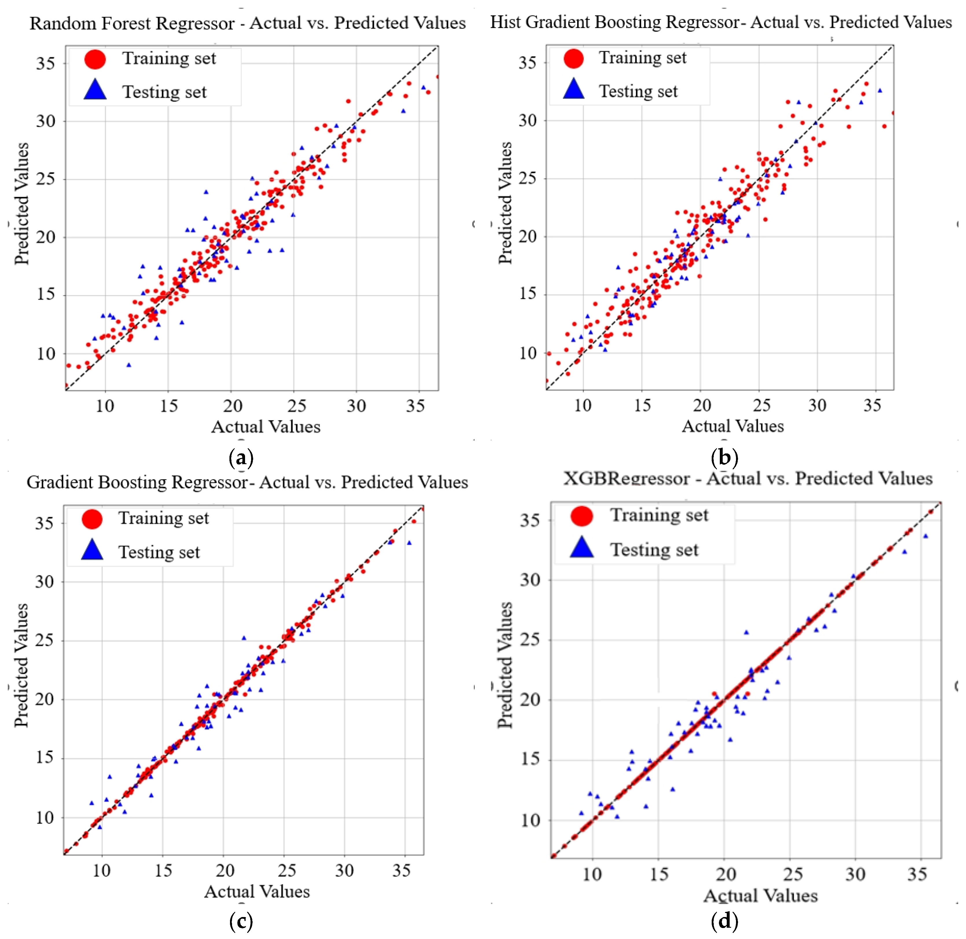
3.1. ML Prediction of UCS Results

In the machine learning training process, hyperparameters are parameters that need to be set before training a model. They cannot be learned during the training process and require manual specification. The selection of hyperparameters is crucial for the performance and training effectiveness of the model, making hyperparameter tuning an essential aspect of machine learning. Among them, “n_estimator” and “max_depth” are two hyperparameters determined later through grid search, with a search range of 1 to 800 for the first and 1 to 20 for the second. The before-and-after settings of hyperparameters for UCS prediction in machine learning models are presented in

Table 3. Results of hyperparameters for UCS prediction.

Model\Hyperparameter	n_estimator (Before/After)	max_depth (Before/After)
Random Forest	100/345	None (no limit)/10
Gradient Boosting Regressor	100/470	3/4
Hist Gradient Boosting Regressor	100 (max_iter)/498	None (no limit)/4
XGBoost	100/119	None (no limit)/4

.

Figure 3 presents a comparison between predicted unconfined compressive strength values and their respective actual values. The actual values are represented on the x-axis, whereas the calculated values are represented on the y-axis. The red dots indicate data points from the training set, the blue triangles represent data points from the test set, and the black dashed line denotes the 45-degree reference line, indicating the scenario where predicted values are equal to actual values [55].

From Figure 3, the data points on each graph closely align with the reference line, indicating a high predictive accuracy for the models. It is observed that both the Random Forest and Hist Gradient Boosting Regressor algorithms exhibit a few test points deviating from the reference line, with this effect being more pronounced in Random Forest. In contrast, Gradient Boosting Regressor and XGBoost demonstrate a better fitting effect.

To quantitatively assess the performance of the ML models, the statistical metrics are illustrated in

Table 4. Specific indicators for each model for UCS prediction.

Variables	Random Forest	Gradient Boosting Regressor	Hist Gradient Boosting Regressor	XGBoost
RMSE	2.4168	1.3085	1.7490	1.5794
MSE	5.8411	1.7121	3.0590	2.4946
MAE	1.9743	1.0320	1.4090	1.2695
R2	0.8176	0.9465	0.9045	0.9221

. This table summarizes the evaluation metrics for four models, reinforcing the conjecture depicted in the diagram. From Table 4, it can be observed that the RMSE of Gradient Boosting Regressor (GBR) is 1.3085, the MSE is 1.7121, the MAE is 1.0320, and the R² is 0.9465. Similar to the visual interpretation presented in Figure 3, the Random Forest, Hist Gradient Boosting Regressor, and XGBoost models exhibit higher values for RMSE, MSE, and MAE, as well as lower values for R². This suggests that their predictive accuracy is lower than that of the GBR model. The superior performance of the GBR is primarily due to its strength in capturing complex, nonlinear interactions among features such as WGP content, alkali dosage, and curing duration. Compared to bagging-based models like Random Forest, GBR builds learners sequentially, allowing error correction at each stage and thus achieving higher predictive accuracy. Its regularisation mechanisms and suitability for small to moderate datasets further enhance its generalisation. In this study, GBR achieved the lowest RMSE (1.3085) and the highest R² (0.9465), confirming its effectiveness for UCS prediction under heterogeneous and weakly correlated input conditions. Consequently, in the pursuit of analytical rigor employing PDP and SHAP methodologies, we leverage Gradient Boosting Regressor.

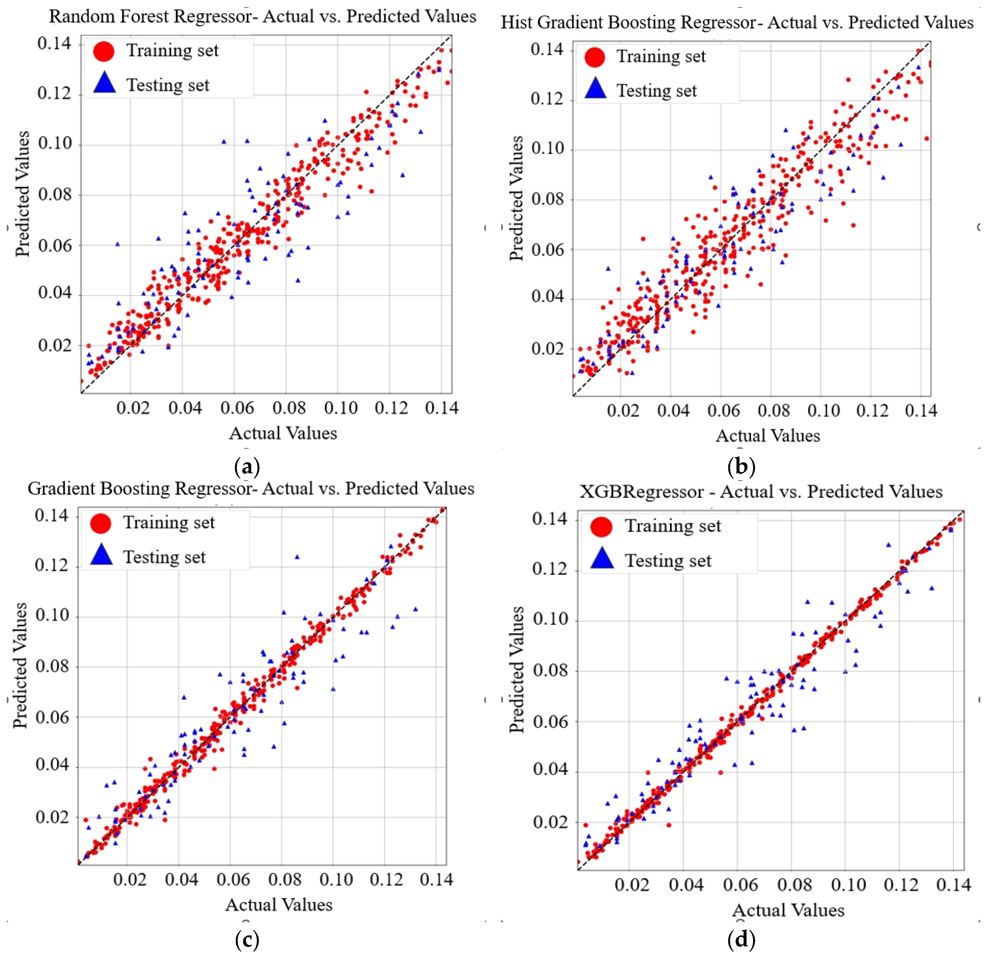
3.2. ML Prediction of ASR Expansion Results

The before-and-after settings of hyperparameters for ASR prediction in machine learning models are presented in

Table 5. Results of hyperparameters for ASR prediction.

Model\Hyperparameter	n_estimator (Before/After)	max_depth (Before/After)
Random Forest	100/116	None (no limit)/13
Gradient Boosting Regressor	100/496	3/4
Hist Gradient Boosting Regressor	100 (max_iter)/646	None (no limit)/8
XGBoost	100/89	None (no limit)/8

.

According to Figure 4, all four graphs can achieve relatively useful predictive results. Among them, the best performers are XGBoost and Gradient Boosting Regressor, as their data points are more closely aligned with the 45-degree reference line. In contrast, Random Forest and Hist Gradient Boosting Regressor are somewhat inferior, as they have some data points that deviate from the reference line.

Table 6. Specific indicators for each model for ASR prediction.

Variables	Random Forest	Gradient Boosting Regressor	Hist Gradient Boosting Regressor	XGBoost
RMSE	0.0166	0.0127	0.0136	0.0101
MSE	0.0003	0.0002	0.0002	0.0001
MAE	0.0134	0.0096	0.0109	0.0080
R2	0.7610	0.8602	0.8396	0.9110

indicates that XGBoost is the best model, with the smallest RMSE, which is 0.0101. The smallest MSE is 0.0001, the minimum MAE is 0.0080, and the R² closest to 1 is 0.9110. The superior performance can be attributed to XGBoost’s ability to effectively model complex nonlinear relationships, which is particularly advantageous given the weak linear correlations observed among the input variables in this study. The ASR dataset involves intricate interactions between features such as curing duration, alkali content, and WGP dosage, which are efficiently captured by XGBoost through its iterative boosting structure and second-order gradient optimisation. Furthermore, the algorithm’s built-in regularisation mechanisms help mitigate overfitting, enhancing its generalisation capability. The model’s robustness performance is further supported by hyperparameter tuning via grid search, allowing parameters to be optimally selected. These characteristics make XGBoost especially well suited for handling the high-dimensional and heterogeneous nature of the ASR dataset, leading to its superior predictive accuracy. Therefore, in the current experiment, XGBoost was used to conduct PDP and SHAP analysis for ASR accordingly.

3.3. Model Interpretability by PDP and SHAP

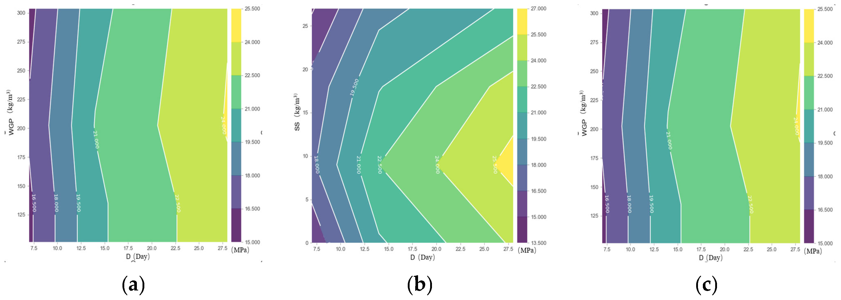
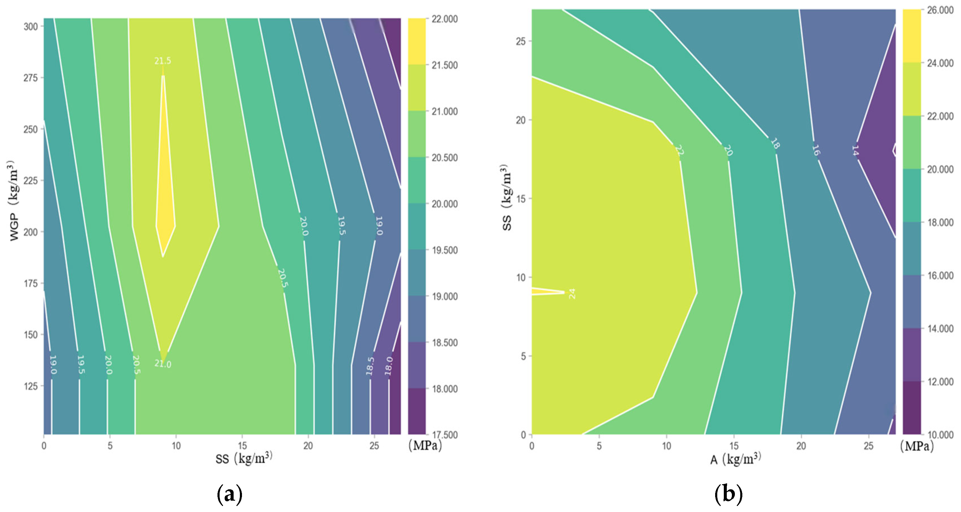
3.3.1. The PDP Explanation Related to the UCS

The contour plots of the obtained PDP reveal evident nonlinear relationships in specific spatial domains. Specifically, the contour profiles display distorted curves rather than straightforward and smooth trends, complicating the interactions within the feature space. Figure 5 depicts the interactive effects of curing duration, alkali, sodium sulfate, and WGP on compressive strength, where the x-axis exhibits the duration and the y-axis illustrates the SS/A/WGP. The duration positively correlates with UCS, regardless of the presence of alkali, sodium sulfate, and WGP. Figure 5a shows that when the curing duration is fixed, UCS slowly decreases as alkali increases. The presence of the alkali additive supplied extra hydroxide ions, increasing the likelihood of the stable structure being disrupted when exposed to high alkali concentrations. Figure 5b indicates a peak in UCS under the combined effect of sodium sulfate and curing duration. In terms of its effectiveness, sodium sulfate can be seen as a result of both alkali stimulation (due to Na⁺) and sulfate stimulation (due to SO4²⁻). In addition to the mentioned alkali activation, the combination of gypsum (CaSO4) with aluminate (C₃A) can form ettringite (AFt) [56]. The moderate content of AFt can boost the density of the mortar and also enhance the initial mechanical strength [57]. Nevertheless, excessive sulfate content invariably results in an overabundance of AFt, leading to a weakened structure and a decrease in the robustness of the mortar [58]. In Figure 5c, it is evident that the variation in WGP yields negligible effects on the unconfined compressive strength.

Figure 6 illustrates the interactive effects of fine aggregate, alkali, sodium sulfate, and WGP on compressive strength. FA is shown along the x-axis, while A/SS/WGP is represented along the y-axis. Figure 6a,b indicates that when either alkali or sodium sulfate remains constant, the variation in fine aggregate does not have a significant effect on compressive strength. The alkali or sodium sulfate content remains invariant, with alterations in compressive strength mainly depending on fine aggregate characteristics and quantity, cementitious material properties, the water–cement ratio, and curing conditions. If these parameters remain consistent across diverse concrete specimens, the variation in compressive strength is expected to be minimal. Figure 6c illustrates that with a gradual increase in the replacement of fine aggregate by waste glass powder, there is an observed trend wherein the compressive strength initially increases, followed by a subsequent decline as WGP content increases and FA content decreases. The optimal replacement ratio is when the amount of WGP is 202.5 kg/m³.

Figure 7 shows the interaction of WGP size, alkali, sodium sulfate, and WGP on compressive strength, with the x-axis being WGP size and the y-axis being A/SS/WGP. Figure 7a–c indicates that as WGP size increases while alkali, sodium sulfate, or WGP remains constant, the compressive strength gradually decreases. Increasing the packing density of smaller reinforcing WGP within the matrix material can result in a more efficient utilization of space, thereby potentially augmenting the material’s compressive strength. This is attributable to the closer stacking arrangement facilitated by the reduced size of WGP. From Figure 7a, there is a clear linear relationship between alkali and WGP size, meaning that as alkali and WGP size increase together, the compressive strength decreases. Adding alkali substances can enhance the compressive strength of composite materials. However, an excessive amount of alkali substances can lead to side effects, such as brittleness or chemical degradation, thereby reducing compressive strength [59]. Figure 7c indicates that a higher proportion of WGP and a smaller WGP size can increase compressive strength [60].

The trends in Figure 6c and Figure 8a are similar, with compressive strength increasing first and then decreasing as WGP replaces sodium sulfate, indicating the presence of an optimal substitution rate. Figure 8b shows that when alkali remains constant, changing sodium sulfate does not significantly affect compressive strength.

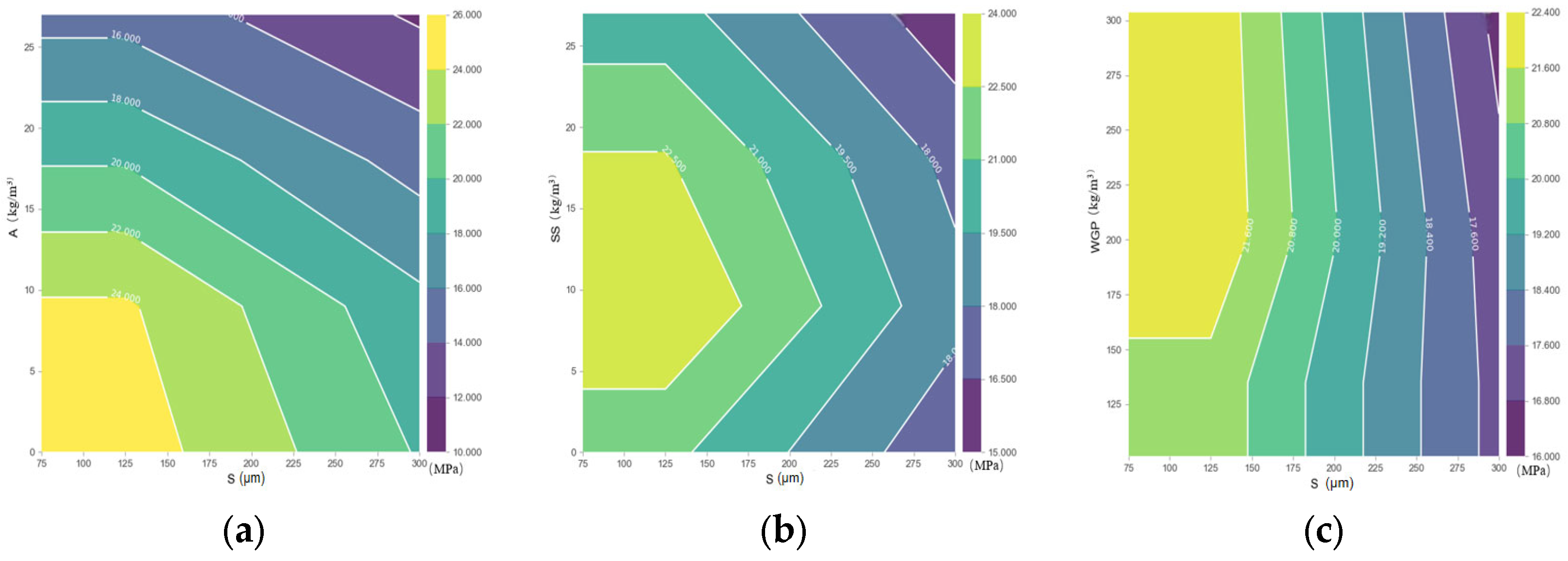
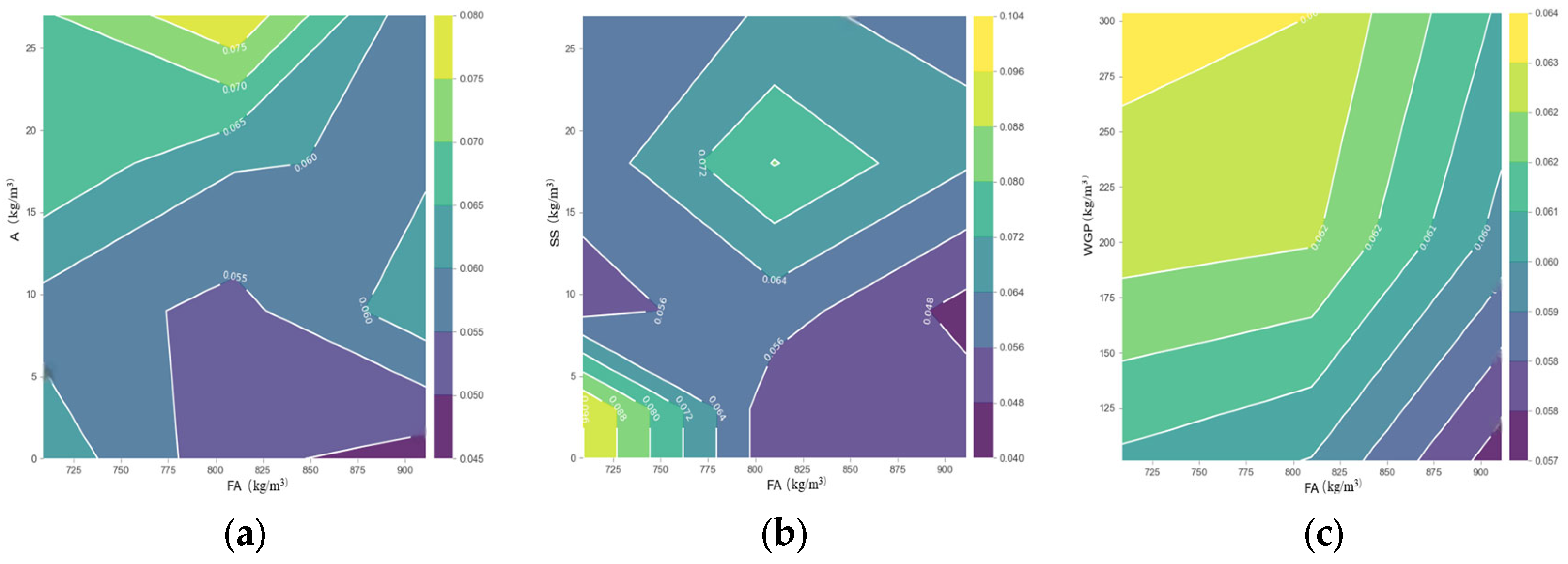
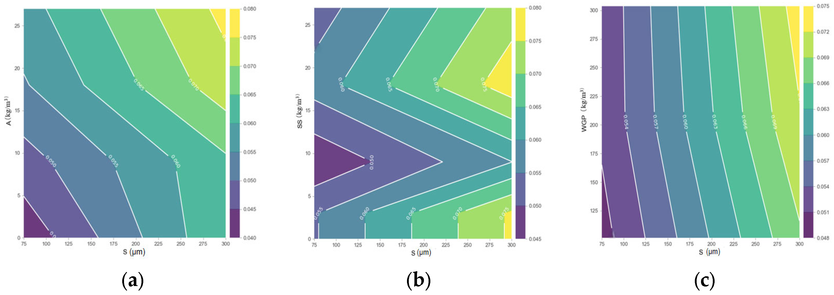
3.3.2. The PDP Explanation Related to the ASR

Figure 9 shows the influence of curing duration, alkali, sodium sulfate, and WGP on ASR, where the x-axis represents curing duration, and the y-axis represents A/SS/WGP. They all exhibit the same trend, with little fluctuation in ASR as alkali, sodium sulfate, or WGP varies when the curing duration remains constant. When alkali, sodium sulfate, or WGP remains constant, ASR increases with an increase in curing duration. Keeping the curing duration constant means that the moisture and temperature conditions in the concrete remain consistent across different experiments. This implies that under a constant curing duration, the effects of alkali, sodium sulfate, WGP, and aggregates on ASR remain relatively constant, resulting in no significant changes in ASR being observed.

The horizontal axis of Figure 10 represents fine aggregate, while the vertical axis represents alkali, sodium sulfate, and WGP, indicating the interactive effects of pairwise factor variations on ASR. Figure 10a indicates that when fine aggregate remains constant, ASR increases with the increase in alkali, reaching its maximum value at an alkali content of 27 kg/m³. Figure 10b indicates that when the fine aggregate is 708.75 kg/m³ and sodium sulfate is less than 5 kg/m³, the ASR value is maximized. Figure 10c shows that when WGP replaces fine aggregate, ASR is enhanced with the decrease in fine aggregate and the increase in WGP.

Figure 11 depicts the impact of changes in alkali, sodium sulfate, WGP, and WGP size on ASR. Figure 11 shows that as WGP size increases, ASR increases when alkali or sodium sulfate or the concentration of WGP remains constant. Larger waste glass powder particles have smaller surface areas, and a relatively smaller surface area means that less surface area can react with the alkaline components in the concrete. Consequently, the diminished susceptibility of larger waste glass powder particles to the influence of alkaline components results in an increased ASR.

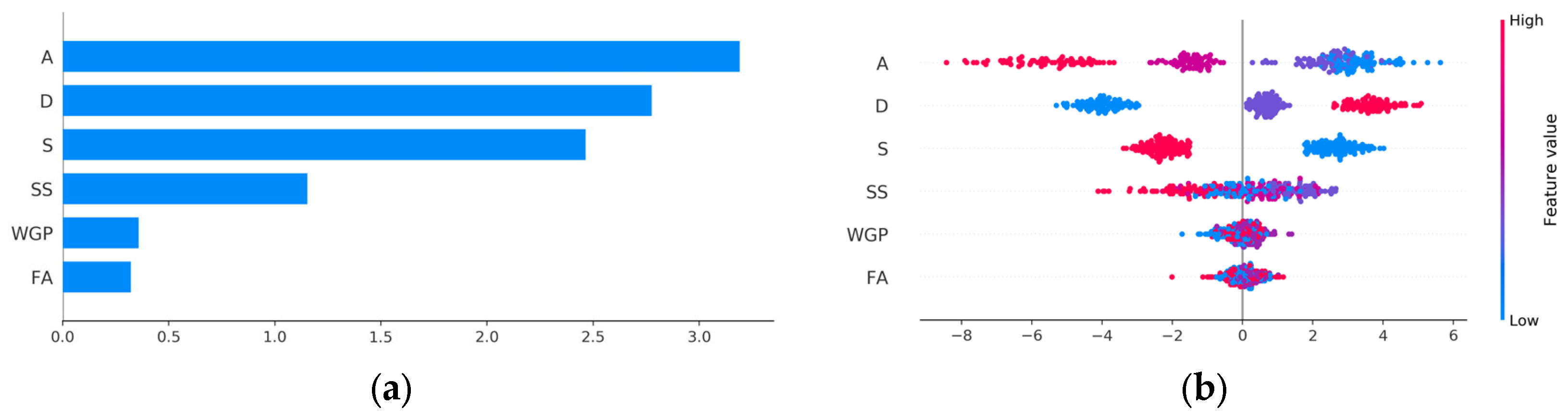
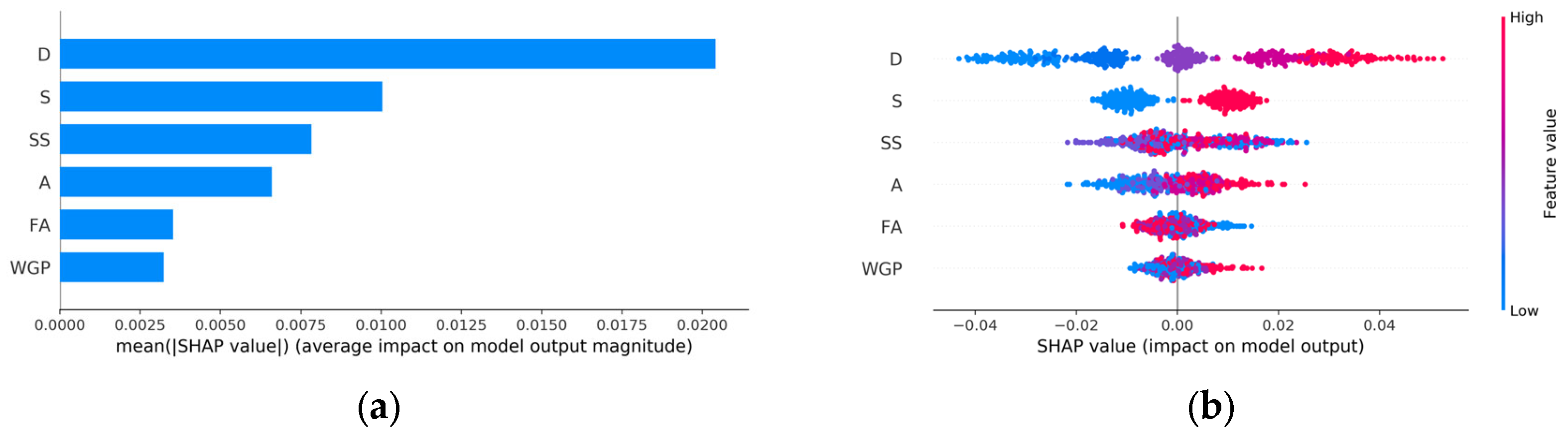
3.3.3. Shapley Additive Explanation (SHAP)

This section will utilize SHAP value summary plots and feature importance bar charts based on SHAP values to analyze the impact of features on the ultimate predictions of UCS and ASR in an ML model.

The SHAP value summary plot illustrates that the overall prediction is influenced by the contribution of each feature [61]. Each point in the plot represents a sample, and the color indicates the size of the characteristic values [62]. Here is a specific explanation. The y-axis represents features ranked from high to low in importance. Each point in the plot represents a feature. The x-axis represents the range of SHAP values. It is a bilateral plot, with negative values on the left and positive values on the right [63]. Each point in the plot represents a sample. The horizontal position of the point represents the SHAP value for that sample. The position of the horizontal line represents the contribution to the overall prediction. The value of the corresponding feature for that sample is represented by the color of the point. Color coding helps us understand the distribution of feature values and their impact on predictions. Through this plot, one can quickly understand which features contribute the most to the overall prediction and observe the distribution of different feature values [64].

The SHAP value feature importance bar chart displays the average impact of each feature on model predictions [65]. Each bar in the chart represents a feature, and the length of the bar represents the average absolute magnitude of its SHAP values [66]. The y-axis represents the features, and each bar in the chart represents a feature. The x-axis represents the average magnitude of SHAP values. The direction of the bars indicates whether a feature has a positive or negative impact on model predictions. Positive impacts are represented by bars extending to the right, while negative impacts are represented by bars extending to the left. This chart allows for an intuitive understanding of which features have a greater influence on model predictions and whether they contribute positively or negatively to the model’s prediction results [67].

The dependency plot between features represents the relationship between the SHAP values of a specific feature (Feature S) and another feature (Feature FA), demonstrating the interaction effects between these two features [68]. The x-axis of the graph shows the values of Feature S, while the y-axis represents the SHAP values of Feature S. SHAP values are a metric used to explain the contribution of Feature S to the model’s predictions. The color of the points on the graph represents the presence of Feature FA. This color guide helps us understand how Feature FA and Feature S are related and how they influence the model’s predictions. Through this graph, insights into the interaction effects between Feature S and Feature FA can be gained, as well as how these two features influence the model’s predictions. This is essential for understanding the mechanisms and key features behind the model’s prediction results [68].

Figure 12 represents a summary of SHAP values related to unconfined compressive strength and a bar chart showing the feature importance of SHAP values. Figure 12a is a bar chart of feature importance for SHAP values, which shows the average influence of alkali, curing duration, WGP size, sodium sulfate, WGP, and fine aggregate on the model’s prediction of UCS value. The SHAP value plot reveals that all features have positive SHAP values, suggesting an increase in the predicted values. The most influential factor in our model’s predictions is the alkali feature, with the curing duration feature coming in second place. Conversely, the influence of the fine aggregate feature on the model’s predictions is minimal. Figure 12b illustrates the impact of each feature on each sample, corresponding to the results in Figure 12a, where the alkali feature contributes the most to the overall prediction. While the size of the WGP has a marginal impact on the overall predictive performance, its significance becomes pronounced when the value is low, particularly in the prediction of specific outcomes.

Figure 13 displays a SHAP value summary chart and a bar graph of feature importance based on SHAP values related to ASR. Figure 13a is a bar chart of feature importance for SHAP values, illustrating the mean influence that each feature has on the model’s predictions of ASR values. Curing duration has the greatest SHAP value impact on ASR, followed by WGP size, and WGP has the smallest impact. When looking at each feature individually, they all positively impact the model predictions of ASR values. Figure 13b is the SHAP value summary plot, displaying the individual impact of every feature on the overall ASR classification. The larger the values of curing duration and alkali, the more positively they influence the SHAP values for ASR. A high value of WGP size has a positive impact, whereas a low value has a negative impact, suggesting a preference for a high WGP size. The influence of sodium sulfate, fine aggregate, and WGP on SHAP values is not consistent and may depend on the experimental conditions.

4. Conclusions

Glass concrete is a type of construction material that combines glass particles or fragments with a cement matrix. This study poses three questions, namely, which algorithm predicts the UCS and ASR of glass concrete more accurately, what is the effect of individual characteristics on the UCS and ASR of glass concrete, and how the prediction output is determined by the contribution of each feature. The main conclusions are as follows:

(1)

GBR achieved the best predictive performance for UCS (RMSE = 1.3085, R² = 0.9465), while XGBoost outperformed others in predicting ASR (RMSE = 0.0101, R² = 0.9110). The superior performance of these two models was attributed to their ability to capture nonlinear feature interactions and their robustness under limited dataset conditions.

(2)

The WGP content showed a nonlinear effect, with an optimal strength observed at 202.5 kg/m³ replacement. Under this condition, UCS values reached 58.6 MPa at 28 days with binary alkali activation, exceeding the 45.3 MPa baseline of the control group. When WGP is 708.75 kg/m³ and the sodium sulfate is less than 5 kg/m³, the alkali–silica reaction value is maximized.

(3)

Through SHAP value analysis, it is evident that the alkali feature significantly influences the unconfined compressive strength prediction, with importance weights up to 0.432. Curing duration ranks as the second most important variable, whereas the fine aggregate feature exhibits the least consequential effect on UCS prediction. When the fine aggregate is 1012.5 kg/m³ and there is no glass powder substitution, the SHAP value is negative, further indicating that glass powder substitution is beneficial for enhancing the positive influence on UCS.

(4)

Curing duration has the greatest impact on the prediction of alkali–silica reaction, while waste glass powder has the smallest impact on ASR prediction. However, when WGP is 303.75 kg/m³, its positive influence on ASR becomes most evident.

Several limitations should be acknowledged in this study. The dataset, although experimentally derived and well structured, remains relatively limited in size, which may restrict the generalizability of the machine learning models. In addition, model evaluation was based solely on internal train–test splits, without external validation using independent datasets. These factors may reduce the robustness and applicability of the results to broader engineering scenarios. Future work should focus on expanding the dataset with field-scale or multi-source experimental data, implementing external validation protocols, and exploring hybrid modeling strategies that combine data-driven algorithms with domain-specific physical principles to improve both predictive accuracy and interpretability.

References

1. Sun, J.; Wang, Y.; Liu, S.; Dehghani, A.; Xiang, X.; Wei, J.; Wang, X. Mechanical, chemical and hydrothermal activation for waste glass reinforced cement. Constr. Build. Mater. 2021, 301, 124361. [Google Scholar] [CrossRef]
2. Singh, A.; Wang, Y.; Zhou, Y.; Sun, J.; Xu, X.; Li, Y.; Liu, Z.; Chen, J.; Wang, X. Utilization of antimony tailings in fiber-reinforced 3D printed concrete: A sustainable approach for construction materials. Constr. Build. Mater. 2023, 408, 133689. [Google Scholar] [CrossRef]
3. Sun, J.; Ma, Y.; Li, J.; Zhang, J.; Ren, Z.; Wang, X. Machine learning-aided design and prediction of cementitious composites containing graphite and slag powder. J. Build. Eng. 2021, 43, 102544. [Google Scholar] [CrossRef]
4. Sun, J.; Wang, X.; Zhang, J.; Xiao, F.; Sun, Y.; Ren, Z.; Zhang, G.; Liu, S.; Wang, Y. Multi-objective optimisation of a graphite-slag conductive composite applying a BAS-SVR based model. J. Build. Eng. 2021, 44, 103223. [Google Scholar] [CrossRef]
5. Feng, W.; Wang, Y.; Sun, J.; Tang, Y.; Wu, D.; Jiang, Z.; Wang, J.; Wang, X. Prediction of thermo-mechanical properties of rubber-modified recycled aggregate concrete. Constr. Build. Mater. 2022, 318, 125970. [Google Scholar] [CrossRef]
6. Sun, J.; Wang, J.; Zhu, Z.; He, R.; Peng, C.; Zhang, C.; Huang, J.; Wang, Y.; Wang, X. Mechanical performance prediction for sustainable high-strength concrete using bio-inspired neural network. Buildings 2022, 12, 65. [Google Scholar] [CrossRef]
7. Zhang, J.; Sun, Y.; Li, G.; Wang, Y.; Sun, J.; Li, J. Machine-learning-assisted shear strength prediction of reinforced concrete beams with and without stirrups. Eng. Comput. 2022, 38, 1293–1307. [Google Scholar] [CrossRef]
8. Sun, J.; Yue, L.; Xu, K.; He, R.; Yao, X.; Chen, M.; Cai, T.; Wang, X.; Wang, Y. Multi-objective optimisation for mortar containing activated waste glass powder. J. Mater. Res. Technol. 2022, 18, 1391–1411. [Google Scholar] [CrossRef]
9. Sun, J.; Wang, Y.; Yao, X.; Ren, Z.; Zhang, G.; Zhang, C.; Chen, X.; Ma, W.; Wang, X. Machine-Learning-Aided Prediction of Flexural Strength and ASR Expansion for Waste Glass Cementitious Composite. Appl. Sci. 2021, 11, 6686. [Google Scholar] [CrossRef]
10. Ren, Z.; Sun, J.; Zeng, X.; Chen, X.; Wang, Y.; Tang, W.; Wang, X. Research on the electrical conductivity and mechanical properties of copper slag multiphase nano-modified electrically conductive cementitious composite. Constr. Build. Mater. 2022, 339, 127650. [Google Scholar] [CrossRef]
11. Zava, A.E.; Apebo, S.N.; Adeke, P.T. The optimum amount of waste glass aggregate that can substitute fine aggregate in concrete. Aksaray J. Sci. Eng. 2020, 4, 159–171. [Google Scholar] [CrossRef]
12. Sun, R.; Wang, D.; Cao, H.; Wang, Y.; Lu, Z.; Xia, J. Ecological pervious concrete in revetment and restoration of coastal Wetlands: A review. Constr. Build. Mater. 2021, 303, 124590. [Google Scholar] [CrossRef]
13. Figueira, R.; Sousa, R.; Coelho, L.; Azenha, M.; De Almeida, J.; Jorge, P.; Silva, C. Alkali-silica reaction in concrete: Mechanisms, mitigation and test methods. Constr. Build. Mater. 2019, 222, 903–931. [Google Scholar] [CrossRef]
14. Adaway, M.; Wang, Y. Recycled glass as a partial replacement for fine aggregate in structural concrete–Effects on compressive strength. Electron. J. Struct. Eng. 2015, 14, 116–122. [Google Scholar] [CrossRef]
15. He, L.; Yin, J.; Gao, X. Additive Manufacturing of Bioactive Glass and Its Polymer Composites as Bone Tissue Engineering Scaffolds: A Review. Bioengineering 2023, 10, 672. [Google Scholar] [CrossRef]
16. Wang, Q.; Yi, Y.; Ma, G.; Luo, H. Hybrid effects of steel fibers, basalt fibers and calcium sulfate on mechanical performance of PVA-ECC containing high-volume fly ash. Cem. Concr. Compos. 2019, 97, 357–368. [Google Scholar] [CrossRef]
17. Açikgenç, M.; Ulaş, M.; Alyamaç, K.E. Using an artificial neural network to predict mix compositions of steel fiber-reinforced concrete. Arab. J. Sci. Eng. 2015, 40, 407–419. [Google Scholar] [CrossRef]
18. Sun, J.; Zhang, J.; Gu, Y.; Huang, Y.; Sun, Y.; Ma, G. Prediction of permeability and unconfined compressive strength of pervious concrete using evolved support vector regression. Constr. Build. Mater. 2019, 207, 440–449. [Google Scholar] [CrossRef]
19. Shariati, M.; Armaghani, D.J.; Khandelwal, M.; Zhou, J.; Khorami, M. Assessment of longstanding effects of fly ash and silica fume on the compressive strength of concrete using extreme learning machine and artificial neural network. J. Adv. Eng. Comput. 2021, 5, 50–74. [Google Scholar] [CrossRef]
20. Feng, D.-C.; Liu, Z.-T.; Wang, X.-D.; Chen, Y.; Chang, J.-Q.; Wei, D.-F.; Jiang, Z.-M. Machine learning-based compressive strength prediction for concrete: An adaptive boosting approach. Constr. Build. Mater. 2020, 230, 117000. [Google Scholar] [CrossRef]
21. Ling, T.-C.; Poon, C.-S. Properties of architectural mortar prepared with recycled glass with different particle sizes. Mater. Des. 2011, 32, 2675–2684. [Google Scholar] [CrossRef]
22. Niu, Y.; Cheng, C.; Luo, C.; Yang, P.; Guo, W.; Liu, Q. Study on rheological property, volumetric deformation, mechanical strength and microstructure of mortar incorporated with waste glass powder (WGP). Constr. Build. Mater. 2023, 408, 133420. [Google Scholar] [CrossRef]
23. Li, Q.; Qiao, H.; Li, A.; Li, G. Performance of waste glass powder as a pozzolanic material in blended cement mortar. Constr. Build. Mater. 2022, 324, 126531. [Google Scholar] [CrossRef]
24. ASTM C305; Standard Practice for Mechanical Mixing of Hydraulic Cement Pastes and Mortars of Plastic Consistency. American Society for Testing and Materials (ASTM): West Conshohocken, PA, USA, 1995.
25. Fall, M.; Célestin, J.; Pokharel, M.; Touré, M. A contribution to understanding the effects of curing temperature on the mechanical properties of mine cemented tailings backfill. Eng. Geol. 2010, 114, 397–413. [Google Scholar] [CrossRef]
26. Lam, C.S.; Poon, C.S.; Chan, D. Enhancing the performance of pre-cast concrete blocks by incorporating waste glass–ASR consideration. Cem. Concr. Compos. 2007, 29, 616–625. [Google Scholar] [CrossRef]
27. ASTM C1260; Standard Test Method for Potential Alkali Reactivity of Aggregates. American Society for Testing and Materials (ASTM): West Conshohocken, PA, USA, 2007.
28. Multon, S.; Sellier, A.; Cyr, M. Chemo–mechanical modeling for prediction of alkali silica reaction (ASR) expansion. Cem. Concr. Res. 2009, 39, 490–500. [Google Scholar] [CrossRef]
29. Chen, Y.; Jia, Z.; Mercola, D.; Xie, X. A gradient boosting algorithm for survival analysis via direct optimization of concordance index. Comput. Math. Methods Med. 2013, 2013, 873595. [Google Scholar] [CrossRef]
30. Zharmagambetov, A.; Gabidolla, M.; Carreira-Perpiñán, M.Ê. Improved boosted regression forests through non-greedy tree optimization. In Proceedings of the 2021 International Joint Conference on Neural Networks (IJCNN), Shenzhen, China, 18–22 July 2021; pp. 1–8. [Google Scholar]
31. Guelman, L. Gradient boosting trees for auto insurance loss cost modeling and prediction. Expert Syst. Appl. 2012, 39, 3659–3667. [Google Scholar] [CrossRef]
32. Rokach, L. Decision forest: Twenty years of research. Inf. Fusion 2016, 27, 111–125. [Google Scholar] [CrossRef]
33. Quinlan, J.R. Induction of decision trees. Mach. Learn. 1986, 1, 81–106. [Google Scholar] [CrossRef]
34. Huang, Y.; Liu, Y.; Li, C.; Wang, C. GBRTVis: Online analysis of gradient boosting regression tree. J. Vis. 2019, 22, 125–140. [Google Scholar] [CrossRef]
35. Liu, P.; Fu, B.; Yang, S.X.; Deng, L.; Zhong, X.; Zheng, H. Optimizing survival analysis of XGBoost for ties to predict disease progression of breast cancer. IEEE Trans. Biomed. Eng. 2020, 68, 148–160. [Google Scholar] [CrossRef] [PubMed]
36. Rodriguez-Galiano, V.F.; Ghimire, B.; Rogan, J.; Chica-Olmo, M.; Rigol-Sanchez, J.P. An assessment of the effectiveness of a random forest classifier for land-cover classification. ISPRS J. Photogramm. Remote Sens. 2012, 67, 93–104. [Google Scholar] [CrossRef]
37. Gayathri, R.; Rani, S.U.; Čepová, L.; Rajesh, M.; Kalita, K. A comparative analysis of machine learning models in prediction of mortar compressive strength. Processes 2022, 10, 1387. [Google Scholar] [CrossRef]
38. Rasheed, Z.; Aravamudan, A.; Sefidmazgi, A.G.; Anagnostopoulos, G.C.; Nikolopoulos, E.I. Advancing flood warning procedures in ungauged basins with machine learning. J. Hydrol. 2022, 609, 127736. [Google Scholar] [CrossRef]
39. Ul Hassan, C.A.; Iqbal, J.; Hussain, S.; AlSalman, H.; Mosleh, M.A.; Sajid Ullah, S. A computational intelligence approach for predicting medical insurance cost. Math. Probl. Eng. 2021, 2021, 1162553. [Google Scholar] [CrossRef]
40. Barnston, A.G. Correspondence among the correlation, RMSE, and Heidke forecast verification measures; refinement of the Heidke score. Weather Forecast. 1992, 7, 699–709. [Google Scholar] [CrossRef]
41. Sutherland, J.; Peet, A.; Soulsby, R. Evaluating the performance of morphological models. Coast. Eng. 2004, 51, 917–939. [Google Scholar] [CrossRef]
42. Zhao, Q.; Hastie, T. Causal interpretations of black-box models. J. Bus. Econ. Stat. 2021, 39, 272–281. [Google Scholar] [CrossRef]
43. Gigerenzer, G.; Brighton, H. Homo heuristicus: Why biased minds make better inferences. Top. Cogn. Sci. 2009, 1, 107–143. [Google Scholar] [CrossRef]
44. Van den Broeck, G.; Lykov, A.; Schleich, M.; Suciu, D. On the tractability of SHAP explanations. J. Artif. Intell. Res. 2022, 74, 851–886. [Google Scholar] [CrossRef]
45. Feyzi, F. CGT-FL: Using cooperative game theory to effective fault localization in presence of coincidental correctness. Empir. Softw. Eng. 2020, 25, 3873–3927. [Google Scholar] [CrossRef]
46. Algaba, E.; Fragnelli, V.; Sánchez-Soriano, J. Handbook of the Shapley Value; CRC Press: Boca Raton, FL, USA, 2019. [Google Scholar]
47. Mitrentsis, G.; Lens, H. An interpretable probabilistic model for short-term solar power forecasting using natural gradient boosting. Appl. Energy 2022, 309, 118473. [Google Scholar] [CrossRef]
48. Lundberg, S.M.; Erion, G.; Chen, H.; DeGrave, A.; Prutkin, J.M.; Nair, B.; Katz, R.; Himmelfarb, J.; Bansal, N.; Lee, S.-I. From local explanations to global understanding with explainable AI for trees. Nat. Mach. Intell. 2020, 2, 56–67. [Google Scholar] [CrossRef]
49. Bulla, C.; Birje, M.N. Improved data-driven root cause analysis in fog computing environment. J. Reliab. Intell. Environ. 2022, 8, 359–377. [Google Scholar] [CrossRef]
50. Yosinski, J.; Clune, J.; Nguyen, A.; Fuchs, T.; Lipson, H. Understanding neural networks through deep visualization. arXiv 2015, arXiv:1506.06579. [Google Scholar]
51. Jas, K.; Dodagoudar, G. Explainable machine learning model for liquefaction potential assessment of soils using XGBoost-SHAP. Soil Dyn. Earthq. Eng. 2023, 165, 107662. [Google Scholar] [CrossRef]
52. Greenwell, B.M.; Boehmke, B.C.; Gray, B. Variable Importance Plots-An Introduction to the vip Package. R J. 2020, 12, 343. [Google Scholar] [CrossRef]
53. Dickinson, Q.; Meyer, J.G. Positional SHAP (PoSHAP) for Interpretation of machine learning models trained from biological sequences. PLoS Comput. Biol. 2022, 18, e1009736. [Google Scholar] [CrossRef]
54. Fetsch, C.R.; DeAngelis, G.C.; Angelaki, D.E. Visual–vestibular cue integration for heading perception: Applications of optimal cue integration theory. Eur. J. Neurosci. 2010, 31, 1721–1729. [Google Scholar] [CrossRef]
55. Abdullah, A.; Jaafar, M.; Taufiq-Yap, Y.; Alhozaimy, A.; Al-Negheimish, A.; Noorzaei, J. The effect of various chemical activators on pozzolanic reactivity: A review. Sci. Res. Essays 2012, 7, 719–729. [Google Scholar] [CrossRef]
56. Liu, C.; Huang, X.; Wu, Y.-Y.; Deng, X.; Zheng, Z. The effect of graphene oxide on the mechanical properties, impermeability and corrosion resistance of cement mortar containing mineral admixtures. Constr. Build. Mater. 2021, 288, 123059. [Google Scholar] [CrossRef]
57. Huseien, G.F.; Shah, K.W.; Sam, A.R.M. Sustainability of nanomaterials based self-healing concrete: An all-inclusive insight. J. Build. Eng. 2019, 23, 155–171. [Google Scholar] [CrossRef]
58. Atiş, C.D.; Bilim, C.; Çelik, Ö.; Karahan, O. Influence of activator on the strength and drying shrinkage of alkali-activated slag mortar. Constr. Build. Mater. 2009, 23, 548–555. [Google Scholar] [CrossRef]
59. Aly, M.; Hashmi, M.; Olabi, A.; Messeiry, M.; Abadir, E.; Hussain, A. Effect of colloidal nano-silica on the mechanical and physical behaviour of waste-glass cement mortar. Mater. Des. 2012, 33, 127–135. [Google Scholar] [CrossRef]
60. Ullah, I.; Liu, K.; Yamamoto, T.; Zahid, M.; Jamal, A. Prediction of electric vehicle charging duration time using ensemble machine learning algorithm and Shapley additive explanations. Int. J. Energy Res. 2022, 46, 15211–15230. [Google Scholar] [CrossRef]
61. Lundberg, S.M.; Erion, G.G.; Lee, S.-I. Consistent individualized feature attribution for tree ensembles. arXiv 2018, arXiv:1802.03888. [Google Scholar]
62. Litovsky, R.Y.; Parkinson, A.; Arcaroli, J. Spatial hearing and speech intelligibility in bilateral cochlear implant users. Ear Hear. 2009, 30, 419. [Google Scholar] [CrossRef]
63. Nie, B.; Xue, J.; Gupta, S.; Patel, T.; Engelmann, C.; Smirni, E.; Tiwari, D. Machine learning models for GPU error prediction in a large scale HPC system. In Proceedings of the 2018 48th Annual IEEE/IFIP International Conference on Dependable Systems and Networks (DSN), Luxembourg, 25–28 June 2018; pp. 95–106. [Google Scholar]
64. Bove, C.; Aigrain, J.; Lesot, M.-J.; Tijus, C.; Detyniecki, M. Contextualization and exploration of local feature importance explanations to improve understanding and satisfaction of non-expert users. In Proceedings of the 27th International Conference on Intelligent User Interfaces, Helsinki, Finland, 22–25 March 2022; pp. 807–819. [Google Scholar]
65. Liu, Y.; Liu, Z.; Luo, X.; Zhao, H. Diagnosis of Parkinson’s disease based on SHAP value feature selection. Biocybern. Biomed. Eng. 2022, 42, 856–869. [Google Scholar] [CrossRef]
66. Caruana, R.; Lou, Y.; Gehrke, J.; Koch, P.; Sturm, M.; Elhadad, N. Intelligible models for healthcare: Predicting pneumonia risk and hospital 30-day readmission. In Proceedings of the 21th ACM SIGKDD International Conference on Knowledge Discovery and Data Mining, Sydney, Australia, 10–13 August 2015; pp. 1721–1730. [Google Scholar]
67. Gomi, H.; Osu, R. Task-dependent viscoelasticity of human multijoint arm and its spatial characteristics for interaction with environments. J. Neurosci. 1998, 18, 8965–8978. [Google Scholar] [CrossRef]
68. Leibold, M.A.; Holyoak, M.; Mouquet, N.; Amarasekare, P.; Chase, J.M.; Hoopes, M.F.; Holt, R.D.; Shurin, J.B.; Law, R.; Tilman, D. The metacommunity concept: A framework for multi-scale community ecology. Ecol. Lett. 2004, 7, 601–613. [Google Scholar] [CrossRef]
Figure 1. The figure of the bivariate plot and correlation coefficient heatmap for the UCS and ASR datasets.
Buildings 15 01866 g001
Figure 2. The distinctive features of WGP with the mean particle size of (a) 300 µm and (b) 75 µm.
Buildings 15 01866 g002
Figure 3. Model performance graphs of four regression models: (a) Random Forest, (b) Hist Gradient Boosting Regressor, (c) Gradient Boosting Regressor, and (d) XGBoost.
Buildings 15 01866 g003
Figure 4. Model performance graphs of four regression models: (a) Random Forest, (b) Hist Gradient Boosting Regressor, (c) Gradient Boosting Regressor, and (d) XGBoost.
Buildings 15 01866 g004
Figure 5. Interactive partial dependence plot with D on the horizontal axis: (a) D-A; (b) D-SS; (c) D-WGP.
Buildings 15 01866 g005
Figure 6. Interactive partial dependence plot with FA on the horizontal axis: (a) FA-A; (b) FA-SS; (c) FA-WGP.
Buildings 15 01866 g006
Figure 7. Interactive partial dependence plot with S on the horizontal axis: (a) S-A; (b) S-SS; (c) S-WGP.
Buildings 15 01866 g007
Figure 8. Interactive partial dependence plot: (a) SS-WGP; (b) A-SS.
Buildings 15 01866 g008
Figure 9. Interactive partial dependence plot with D on the horizontal axis: (a) D-A; (b) D-SS; (c) D-WGP.
Buildings 15 01866 g009
Figure 10. Interactive partial dependence plot with FA on the horizontal axis: (a) FA-A; (b) FA-SS; (c) FA-WGP.
Buildings 15 01866 g010
Figure 11. Interactive partial dependence plot with S on the horizontal axis: (a) S-A; (b) S-SS; (c) S-WGP.
Buildings 15 01866 g011
Figure 12. Feature importance bar charts based on SHAP values and SHAP value summary plot to UCS: (a) Average SHAP Value per Feature; (b) SHAP Summary: Impact and Value Distribution.
Buildings 15 01866 g012
Figure 13. Feature importance bar charts based on SHAP values and SHAP value summary plot to ASR: (a) Average SHAP Value per Feature; (b) SHAP Summary: Impact and Value Distribution.
Buildings 15 01866 g013