Abstract
Landslides triggered by extreme rainfall often cause severe casualties and property losses. Therefore, it is essential to accurately assess and predict building vulnerability under landslide scenarios for effective risk mitigation. This study proposed a quantitative framework for vulnerability assessments of structures. It integrated extreme rainfall analysis, landslide kinematic assessment, and the dynamic response of structures. The study area is located in the northern mountainous region of Tianjin, China. It lies within the Yanshan Mountains, serving as a key transportation corridor linking North and Northeast China. The Sentinel-1A satellite imagery consisting of 77 SLC scenes (from October 2014 to November 2023) identified a slow-moving landslide in the region by using the SBAS-InSAR technique. High-resolution topographic data of the slope were first acquired through UAV-based remote sensing. Next, historical rainfall data from 1980 to 2017 were analyzed. The Gumbel distribution was used to determine the return periods of extreme rainfall events. The potential slope failure range and kinematic processes of the landslide were then simulated by using numerical simulations. The dynamic responses of buildings impacted by the landslide were modeled by using ABAQUS. These simulations allowed for the estimation of building vulnerability and the generation of vulnerability maps. Results showed that increased rainfall intensity significantly enlarged the plastic zone within the slope. This raised the likelihood of landslide occurrence and led to more severe building damage. When the rainfall return period increased from 50 to 100 years, the number of damaged buildings rose by about 10%. The vulnerability of individual buildings increased by 10% to 15%. The maximum vulnerability value increased from 0.87 to 1.0. This model offers a valuable addition to current quantitative landslide risk assessment frameworks. It is especially suitable for areas where landslides have not yet occurred.
1. Introduction
Rainfall-induced landslides are one of the most devastating natural hazards globally, presenting persistent risks to building safety and the sustainable development of mountainous communities [1,2,3]. In recent years, the increasing frequency of extreme rainfall events due to climate change has significantly escalated the abundance and severity of rainfall-induced landslides [4,5,6]. Due to its complex geological conditions and distinct monsoonal precipitation characteristics, China is a high-risk area for such disasters [7,8]. During a landslide event, high-speed impact, debris burial, and dynamic erosion can lead to structural damage and functional failure of buildings. According to the EMDAT disaster database, the extent of building damage caused by landslides is among the highest globally, with China experiencing particularly severe losses [9]. This reality underscores the urgent need for quantitative vulnerability assessments of buildings under extreme rainfall scenarios.
At slope/site scales, landslide hazard assessment is an important foundation for the vulnerability assessment of buildings. A well-established framework has been developed regarding this topic, among which landslide mechanisms related to the rainfall infiltration should be stated first [10,11]. At present, the key factors affecting rainfall-induced landslides have been widely studied, including geological conditions, material properties, rainfall indicators (intensity, duration, threshold, etc.), and engineering activities (e.g., reservoir impoundment) [12,13,14]. Within this framework, various techniques have been developed and applied, mainly including laboratory tests [15], in situ monitoring [16], numerical simulation [17], model tests [18], statistical analysis [19], and so on. Therefore, the relationship between rainfall and landslide occurrence has been relatively clear in terms of the triggering mechanism. The second key point for landslide hazard assessment is the landslide kinematic process, which is normally used to clarify the probability of whether a landslide can reach the elements at risk, namely by so-called runout analysis [20]. Regarding this topic, numerical analysis is generally the methods of choice in the literature, including but not limited to finite element method (FEM) [16], discrete element method (DEM) [21], discontinuous deformation analysis (DDA) [22], finite difference method (FDM) [23], material point method [24], and coupling methods. These techniques can reveal some critical indicators during landslide movement that are rather important for assessments of building vulnerability. However, it should be noticed that most studies mentioned above are associated with historical landslide events, meaning that sufficient information can be acquired for geological modeling. However, this is commonly impossible for those landslide hazards that have not yet occurred. Many of them only conduct limited investigations, and sparse data fail to support accurate modeling. In particular, failure ranges or magnitudes of slopes depend much on rainfall scenarios, but few studies have considered variable landslide volumes. Regarding this issue, the ABAQUS software V2022 was utilized to identify the failure range through the analysis of plastic zone distribution.
Vulnerability is typically quantified on a continuous scale from 0 (no damage) to 1 (total loss) to represent the degree of damage sustained by buildings under a given hazard intensity [25]. The assessment process involves multiple critical factors, including landslide frequency and magnitude, exposed element types, building structures and materials, and so on [26,27]. Hence, it is important to obtain critical parameters and integrate different components into vulnerability calculation. Generally speaking, there are three kinds of methods to achieve physical vulnerability of buildings, namely indicator-based methods, data-driven methods, and mechanism-based methods [28]. The first method determines vulnerability based on weighted factors considering element characteristics and landslide intensity [29,30]. Data-driven methods can establish the relationship between landslide intensity and building damages via regression analysis. Hence, it is important to obtain sufficient information related to landslide magnitude and building damages of the past events [31]. However, both methods carry few physical interaction mechanisms between rock–soil masses and structures; thus, they are more of a qualitative approach. Under this context, their outcomes are empirical vulnerability functions or curves, which normally fail to characterize the dynamic responses of a given building [32]. On the contrary, the mechanism-based approaches can reveal a single building response under the mass impact, thus making it possible to achieve quantitative vulnerability assessment. Within this framework, some beneficial attempts have been made, especially those based on numerical simulations [33] and laboratory model tests [34]. However, as stated in the literature [28], significant research gaps still exist in regard to the progressive failure modes of buildings under landslide impact. This is mainly because the analysis for the landslide kinematic process and the impacts of rock–soil masses on structures are commonly split. In this study, we employed various numerical simulation techniques to integrate the two procedures and achieve the dynamics of building damage assessment via time.
The most important objective of the present study is to propose a quantitative model for the vulnerability assessment of buildings within the framework of landslide risk assessment. Many potential landslide hazards exist in mountainous areas, but it is difficult to accurately predict the losses of structures once the slopes initiate. Under the context of this issue, our main objectives include the following: (i) to predict the failure range and probability of landslides under specific rainfall scenarios through numerical simulations; (ii) to assess the post-failure landslide motion and extract key dynamic parameters; and (iii) to simulate the impact of landslides on buildings using ABAQUS and quantify building vulnerability. Given that current studies mostly focus on the back-analysis of building vulnerability during historical landslide events, the expected outcomes of this study will contribute more to the risk reduction and mitigation for those potential hazards.
2. Study Area
2.1. General Setting
The potential landslide site of the Gouhebei Landslide (GHBL) is located in Gouhebei Village, Jizhou District, Tianjin City, China (Figure 1), with its central geographical coordinates approximately 117°18′36″ E and 40°07′23″ N. The landslide’s elevation varies from 410 m to 273 m, with its rear edge situated along the mountain ridge and its front edge gradually extending into the residential area of Gouhebei Village, creating a maximum elevation difference of about 140 m. The landslide body exhibits an elongated shape, with a longitudinal length of about 420 m, a width of approximately 130 m, and a total planar area of around 0.05 km². The overall slope inclination is approximately 30°, indicating a relatively steep terrain. According to geological surveys, the exposed strata within the landslide area mainly include artificial fill (Qme), Quaternary Holocene alluvial deposits (Q4del), Quaternary Holocene colluvial–alluvial deposits (Q4dl+pl), Upper Pleistocene residual-slope deposits (Q3el+dl), and the Jixian System Yangzhuang Formation (Jxy) (Figure 1). The lithology of these strata primarily consists of limestone, sandstone, and dolomite, characterized by a distinctly layered structure. The degree of rock weather varies from highly weathered to moderately weathered. Some rock layers contain dolomitic bands, with thicknesses ranging from approximately 0.2 to 0.3 m. The rock strata dip at 24° ∠ 31°, with two predominant joint sets oriented at 114° ∠ 85° and 72° ∠ 81°. These geological characteristics suggest that the stability of the landslide body is influenced by the structural configuration of the rock layers and the development of fractures, potentially increasing the likelihood of landslide occurrence.
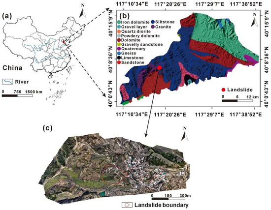
Figure 1.
(a) Location of the Tianjin City in China; (b) the lithology map of the Jizhou District, where the red dot shows the specific location of the Gouhebei landslide; and (c) The orthophoto image of the Gouhebei village, where the boundary of the landslide is clarified.
The region experiences a warm temperate, semi-humid continental monsoon climate with distinct seasonal variations, characterized by hot and rainy summers and cold, dry winters. The multi-year average precipitation is 678.6 mm, with significant interannual variability. The distribution of precipitation is highly uneven, with over 80% occurring between June and September, and July and August receive the highest rainfall, with monthly precipitation in certain years approaching the total annual precipitation. For example, in July 1978, the total monthly precipitation reached 538.2 mm, accounting for 79% of the annual average. Additionally, short-duration heavy rainfall events are prominent, as exemplified by the extreme rainfall on 24 July 1985, when the hourly precipitation reached 71.2 mm. These precipitation characteristics serve as critical triggering factors for landslides, particularly during extreme rainfall events, which significantly increase the probability of landslide hazards.
2.2. Landslide Details
In this study, SBAS-InSAR technology was employed to monitor the surface deformation of the landslide area. The Sentinel-1A satellite imagery, consisting of 77 SLC scenes acquired between 22 October 2014 and 16 November 2023, was downloaded from the ESIS software platform V017. The imagery was obtained using the C-band (wavelength: 3.1 cm) with an incidence angle of 30.66° and processed using Copernicus DEM data with a resolution of 30 m for differential interferometric analysis. Based on temporal and spatial baseline constraints, suitable interferometric image pairs were selected and imported into the processing environment. Subsequently, the imagery was clipped according to the study area’s geographic coordinates to enhance data accuracy, and the clipped data were used for time-series analysis to extract the temporal evolution of surface deformation. To ensure monitoring accuracy, ascending and descending track data were cross-validated, and precise orbital ephemeris data (POD) provided by ESA were applied for orbital correction. The results (Figure 2) indicate that GHBL and its surrounding areas exhibit significant surface deformation within the study area, with deformation magnitudes generally ranging from 50 to 100 mm over the past decade. Field investigations reveal that due to the instability of Quaternary shallow deposits and strong bedrock weathering, small-scale collapses and accumulated layer failures have occurred in certain areas. Consequently, in May 2024, local authorities designated this area as a geological-hazard early warning site and installed professional monitoring instruments to observe surface deformation (Figure 2). It can be seen from the monitoring data that rainfall is mainly concentrated in May–July, accounting for a larger proportion of the annual rainfall. At the same time, with the increase in rainfall, soil moisture and soil pressure also increase, aggravating the development of cracks. In summary, the surface deformation of the landslide has become increasingly pronounced. Hence, the slope poses a high risk of instability and failure, particularly under extreme rainfall conditions.
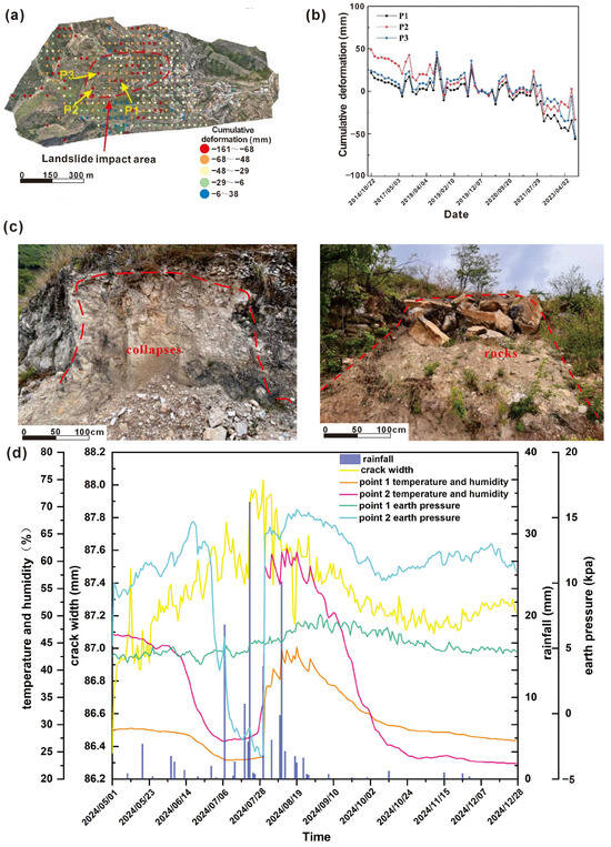
Figure 2.
(a) InSAR deformation distribution map of the GHBL hazard area, (b) InSAR cumulative deformation of characteristic points in the GHBL, (c) small-scale collapses in the field, and (d) instrument data from landslide-monitoring points in Gouhebei village.
3. Data and Methods
3.1. Modeling Framework
This study integrated extreme rainfall scenarios, topographic data, stability analysis, kinematic simulations, and building vulnerability calculation to establish a systematic vulnerability assessment framework. It comprised several key steps (Figure 3): (i) Extreme rainfall scenarios for different periods were computed using the Gumbel distribution to simulate the impact of varying rainfall conditions on landslide activity. (ii) Unmanned aerial vehicle (UAV) remote-sensing technology was utilized for on-site data collection, capturing high-resolution topographic information and producing a digital elevation model (DEM) as the primary dataset for subsequent landslide simulations. (iii) The landslide process was simulated using ABAQUS and GeoStudio to calculate the stability and failure range. (iv) A particle-flow code (PFC) was employed for landslide simulation and kinematic processes. (v) Based on the PFC dynamic simulation results, the impact load was quantified and incorporated into the ABAQUS structural simulation to assess the vulnerability of buildings in the affected area. (vi) The quantified building vulnerability results were integrated into GIS software V10.2 to generate a vulnerability distribution map, visually representing the spatial extent of landslide impacts and the severity of structural damage.
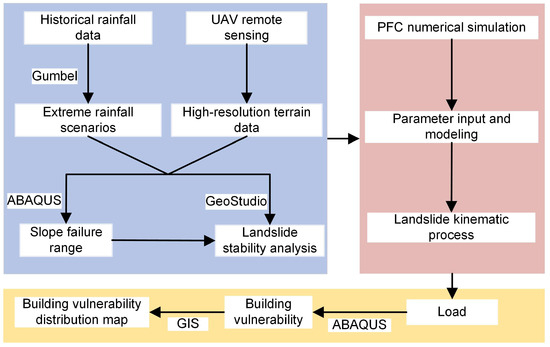
Figure 3.
The proposed methodological framework of this study for landslide hazard assessment.
It should be noted that the proposed framework is flexible, which is mainly used to exhibit how to achieve quantitative vulnerability assessment within the current landslide risk assessment framework. All the approaches mentioned above, including UAV, Gumbel, ABAQUS, GeoStudio, and PFC, are the measurements, instead of the aims. In other words, users can easily adjust the specific methods to generate a new assessment route without any potential conflicts or contradictions, as long as the data-format conversation between their methodologies is possible.
3.2. Extreme Rainfall Scenario
The stability of rainfall-induced landslides varies significantly with rainfall intensity and duration [35]. Additionally, landslide kinematic processes exhibit substantial differences, leading to varying degrees of building damage. Therefore, selecting an appropriate statistical method for analyzing rainfall intensity is essential. Currently, commonly used methods for extreme rainfall probability estimation include the Gumbel distribution, Weibull distribution, log-normal distribution, Pearson Type-III distribution, and three-parameter inverse gamma distribution [10,36]. Since the Gumbel distribution is particularly effective in assessing the probability of one or more rainfall events exceeding a given threshold within a specified time range and estimating the rainfall return period [37], this distribution is widely used to describe the probability of extreme events occurring in a specific period and region. In this study, the Gumbel distribution was selected for rainfall event probability analysis.
In this study, long-term historical rainfall data (1980–2017) were utilized to generate extreme rainfall values for the study area (Figure 4). During data analysis, particular attention was given to the spatiotemporal characteristics of rainfall distribution. The analysis indicated that three consecutive days of rainfall are the most frequent extreme rainfall events during the rainy season in the study area. Therefore, this study selected the maximum three-day consecutive precipitation for each month as a representative extreme rainfall event and further analyzed its return period.
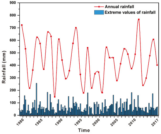
Figure 4.
Annual rainfall and monthly maximum 3-day consecutive rainfall in the study area (January 1980–December 2017).
The probability density function (PDF) and cumulative distribution function (CDF) of the Gumbel distribution are expressed as follows:
The relationships between the mean value (μ) and the location parameter (β) and scale parameter (α) are given as follows:
Among them, α and β can be estimated using the maximum likelihood method.
3.3. UAV Remote Sensing
In this study, a DJI Mavic 3E UAV equipped with a 20 MP APS-C sensor high-resolution camera and an RTK positioning system was utilized to conduct refined remote-sensing modeling of the landslide terrain. First, the flight area was delineated using Google Earth and imported as a KMZ file. Based on terrain undulations, the flight parameters were set with a forward overlap of 83%, a side overlap of 75%, and a flight altitude ranging from 100 to 300 m (corresponding to a ground sampling distance, GSD = H/37), ensuring precise image matching in steep areas. During the flight, an autonomous flight path-planning technique was employed to achieve full aerial coverage of both the landslide-affected core area and adjacent regions. In the data-processing stage, Pix4Dmapper V4.3 software was used for fully automated processing, including image-distortion correction, radiometric calibration, POS-assisted aerial triangulation, and dense point cloud generation. A free-network bundle adjustment combined with ground control point (GCP) absolute orientation was applied to ensure high-precision georeferencing, resulting in the final outputs of an orthophoto mosaic (DOM) and a 3D geological model. Additionally, to address areas with significant landslide deformation, a high-overlap aerial survey strategy (forward/side overlap > 75%) and a GCP-free method (achieving an accuracy of up to 2× GSD) were employed. These techniques effectively mitigated technical challenges associated with large elevation differences and indistinct terrain features, providing a high-precision spatial data foundation for landslide stability analysis and disaster assessment.
3.4. Landslide Stability Analysis
3.4.1. Landslide Failure Range Analysis Based on ABAQUS
Prediction of landslide instability and failure range is crucial for landslide hazard assessment, since they are associated with landslide intensity [38]. The potential failure range of a slow-moving landslide depends much on triggering conditions. However, most studies always assume that landslides will slide with fixed surfaces, which are normally determined based on in-site investigations or geophysics.
In this study, ABAQUS was employed to conduct seepage–stress coupling analysis, simulating landslide instability and failure processes under different rainfall scenarios. The landslide failure extent was determined using plastic zone distribution contour maps. First, based on the topography and geological cross-sections, a 2D model was constructed to accurately represent the landslide’s geometric characteristics (Figure 5). In terms of material parameter determination, soil information obtained from field investigations, such as soil type and unit weight, was first recorded. Local authorities conducted laboratory tests to determine values of mechanical and hydraulic parameters at specific sites. Combined with the recommended values for geotechnical materials provided in the ABAQUS User Manual [39], the input parameters were assigned (Table 1). Specifically, the physical and mechanical properties of the landslide mass, including density, elastic modulus, Poisson’s ratio, and compressive strength—as well as hydraulic parameters such as permeability coefficient and porosity—were defined accordingly. For boundary conditions, in the rainfall infiltration analysis, the upper boundary of the slope was set as the rainfall boundary, while other boundaries were defined as free boundaries. In the deformation analysis, only the gravity direction was maintained as the free boundary, with the lower-left corner of the cross-section set as the coordinate origin. Subsequently, based on the rainfall data from Section 3.2, rainfall scenarios with 50-year and 100-year return periods were considered. These rainfall conditions were incorporated into the model through seepage analysis to simulate the impact of rainfall infiltration on landslide stability. Rainfall intensity distribution and duration were applied as external loads on the model boundaries to represent the continuous infiltration process. Changes in pore water pressure and hydraulic head distribution due to precipitation influenced the overall stability of the landslide body. Finally, plastic zone distribution contour maps were extracted to identify areas experiencing plastic deformation or failure under specific rainfall conditions. Based on the distribution of plastic zones, the landslide failure extent was further calculated and predicted. By analyzing the formation process of instability and failure zones, potential landslide hazard areas were identified, providing a scientific basis for landslide disaster assessment.
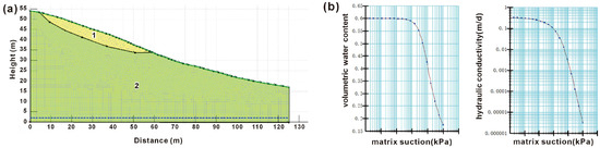
Figure 5.
The settings for the stability evaluation in GeoStudio: (a) the constructed geological model and (b) the hydrological parameter configurations.

Table 1.
Input parameters of slope materials used for plastic deformation simulation in ABAQUS.
3.4.2. Landslide Stability Analysis Based on GeoStudio
Landslide hazard assessment requires calculating the failure probability of landslides under specific rainfall conditions. Therefore, this study employed GeoStudio for numerical simulation to evaluate landslide stability and quantify failure probability. The SLOPE/W module was used for landslide stability analysis, enabling probability calculations under different conditions, making it particularly suitable for disaster assessment and mitigation planning [40,41]. First, a landslide model was established based on the geological conditions of the study area, and the mesh was generated using quadrilateral and triangular elements with a global element size of 0.5 m, resulting in a model comprising 5027 nodes and 4846 elements. Based on ABAQUS analysis results, the plastic zone was defined as the sliding surface, and the geological model was divided into two parts: the sliding mass and the sliding bed, each assigned distinct material properties (Table 2). Regarding boundary conditions, in rainfall infiltration analysis, the upper slope was set as the rainfall boundary, while the remaining areas were defined as free boundaries; in deformation analysis, the surrounding boundaries of the slope were fixed (Figure 5). Subsequently, the SEEP/W module was used to conduct seepage simulations to analyze permeability characteristics under different rainfall conditions. Rainfall intensity and duration were set to match the ABAQUS analysis, and SEEP/W outputs the water flow distribution and hydraulic head variations within the landslide mass. Based on the results of SEEP/W seepage analysis, the SIGMA/W module was employed to analyze slope deformation characteristics, examining slope deformation behavior under different rainfall scenarios. Based on seepage and deformation analysis, the SLOPE/W module was used for slope stability analysis to determine the location of the sliding surface and evaluate slope stability. The entry and exit points of the sliding surface were identified to further analyze the failure mechanisms of the slope. Additionally, the landslide failure probability was calculated, and the safety factor distribution was derived to quantify landslide failure risk.
Table 2.
Input parameters of the sliding mass and bedrock for slope stability analysis in GeoStudio.
3.5. Landslide Kinematic Process
After determining the landslide failure extent and its instability probability, it was necessary to further analyze the kinematic characteristics of the sliding mass to identify its final impact range. Since landslides and debris flows were distinct types of geological hazards with different triggering mechanisms and movement characteristics, their motion processes require different evaluation methods. The PFC model, by simulating particle interactions, could accurately reproduce the behavior of granular materials in complex geological problems, making it particularly suitable for the dynamic analysis of landslides and rockfalls [42,43]. Its advantages included accurate simulation of nonlinear behavior, adaptability to complex boundary conditions, capability to handle intricate geological problems, efficient computation, and high-quality visualization, making it widely applicable in landslide risk assessment, disaster early warning, and mitigation planning [44,45]. Therefore, in this study, the PFC discrete element method was employed to simulate and evaluate the landslide movement process.
Based on the landslide failure extent, we delineated the sliding mass and sliding bed, entered the relevant parameters, and then imported them into PFC2D for simulation (Table 3). The landslide model was configured according to different rainfall scenarios, where the average thickness of the plastic zone was 8 m under the 50-year return period rainfall scenario and 10 m under the 100-year return period scenario. Particle generation was performed using both regular generation and random generation methods, with a porosity of 0.2 applied in the collapse area for random particle generation. The particle radius was set between 0.4 and 0.7 m, while for the sliding bed, the same generation method was used with a particle radius of 0.5–0.6 m, resulting in 6848 particles in total. During the landslide motion process, four monitoring particles were placed at different locations within the collapse area to track kinematic parameters, including sliding velocity, movement duration, travel distance, and particle velocity (Figure 6). In the 3D modeling process, topographic factors such as elevation, slope, and aspect were incorporated into 3ds Max to generate the landslide surface model. The expansion method and rainfall method were applied to simulate particle filling in the landslide source area. The sliding bed was modeled as a rigid wall, with the landslide mass and sliding bed forming a complex enclosed surface, in which particles were placed with a porosity of 0.2 and a radius range of 0.4–0.7 m, ultimately generating 7648 particles. The ball-wall method was used to construct the geological model of the landslide, reducing the total number of particles to optimize computational efficiency (Figure 6).
Table 3.
The material parameters used for the landslide runout simulation in PFC.
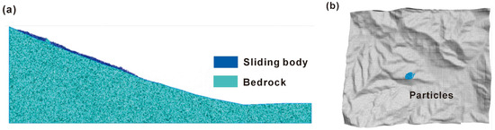
Figure 6.
The geological models of the GHBL in PFC: (a) 2D and (b) 3D.
3.6. Building Vulnerability Assessment
ABAQUS is a high-performance finite element analysis software with powerful engineering simulation capabilities, widely used for numerical modeling of various engineering materials and structures [46,47]. Its comprehensive element library and material model database support the simulation of reinforced concrete, soil, rock, metal, rubber, polymer materials, and composites, enabling the solution of problems ranging from linear analysis to complex nonlinear behaviors [48,49]. In addition to its extensive applications in structural analysis (stress/displacement) in civil engineering, ABAQUS is also utilized in geomechanics (fluid infiltration/stress coupling analysis), mass diffusion, electrothermal coupling, acoustic analysis, heat conduction, and piezoelectric medium analysis across multiple engineering disciplines [50,51]. In this study, the ABAQUS/CAE built-in modeling tool was employed to conduct numerical simulations of building deformation under geohazard impact loads, aiming to analyze the structural response and damage patterns of buildings subjected to landslide forces.
First, the fundamental physical characteristics of landslide bodies and affected buildings within the study area were collected to provide essential input data for numerical simulation. Subsequently, dynamic parameters such as flow depth and velocity at different time steps—captured as the landslide reaches the buildings—were extracted from the landslide simulation results. Using these parameters, the impact load exerted by the landslide on the buildings was calculated based on an impact load equation. The resulting loads were then imported into the ABAQUS/CAE software V2022 for structural deformation simulation.
To quantitatively assess the vulnerability of buildings, this study adopted the Concrete Damage Plasticity (CDP) model. CDP is a widely used constitutive model in ABAQUS for simulating the nonlinear behavior of concrete. It accounts for distinct failure mechanisms under tension and compression, including cracking, crushing, damage evolution, and irreversible plastic strain, making it an advanced and practical damage–plasticity coupled model [52,53]. In ABAQUS, the CDP model outputs result in contour plots of concrete stiffness degradation. By analyzing the number of failed mesh elements in the building model at each time step, a function curve of stiffness degradation rate versus time was plotted. The ratio of failed mesh elements to the total number of elements at time step i was defined as Pi. The curve of Pi versus i was then plotted, and the first inflection point—where the slope of the curve changes significantly—was identified. The vulnerability value of the building at this point was defined as 1, and the corresponding Pi,max was recorded. Finally, the vulnerability value, V, at any given time step, i, was calculated using the following formula:
where V represents the extent of damage sustained by the building under a given geohazard intensity. When V is 0, the building remains intact; as V increases, the damage sustained due to landslide impact grows; and when V is 1, the building is completely damaged.
Through extensive field investigations and interviews, we found that the landslide was in a village, where slope-cut housing constructions were widespread. A main road leading to a scenic area nearby ran through the landslide toe, which has further caused the guesthouses to be densely distributed during the past decade. All of these buildings within the potentially affected area have a frame structure. During the field surveys, we documented detailed information on the buildings, including the number and heights of stories. In the simulation, each individual building within the potentially affected area was modeled to obtain corresponding vulnerability estimates. However, due to the length limitation, it was not possible to present all the results in detail. Instead, a two-story building was taken as an example for illustration, since this height was the most common within the landslide area.
As seen in Figure 7, the example building was a two-story guesthouse with a length of 16.4 m and a width of 7.7 m, using a three-bay reinforced concrete frame structure. The columns have cross-sections of 500 × 500 mm, the beams have cross-sections of 500 × 600 mm, and the slab thickness is 150 mm. All components were cast in place. Each column is reinforced with eight Φ16 longitudinal steel bars; beams are reinforced with eight Φ14 bars, along with two additional waist reinforcements. Slab reinforcement was designed according to standard specifications. Stirrups are Φ10@200 mm, with end regions additionally reinforced. All steel bars used were grade HRB500, and the concrete was grade C30. Based on this structural information, the building was modeled in ABAQUS, with material properties defined accordingly. The input parameters for the Concrete Damage Plasticity (CDP) model were selected according to the available literature [54,55,56]. The structure was assembled, and appropriate contact interactions were defined. The load–time curve was then applied to the building’s columns, while fully fixed boundary conditions were imposed at the column bases to realistically represent ground constraints. During the simulation, concrete was modeled using three-dimensional 8-node linear brick elements with reduced integration (C3D8R), and the reinforcing bars were modeled using three-dimensional 2-node truss elements (T3D2), from the general beam element family.
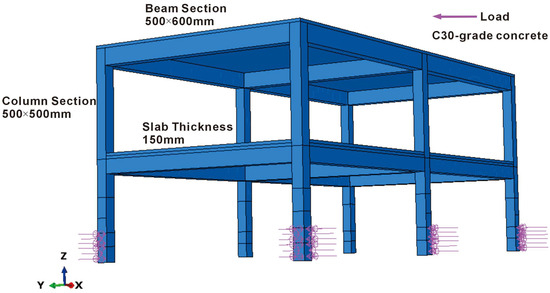
Figure 7.
The schematic diagram of the example building and its impact loading in ABAQUS. The building has a two-story height and a three-bay RC frame structure.
4. Results
4.1. Landslide Failure Analysis
4.1.1. Landslide Failure Range
Based on the Gumbel distribution function, the maximum three-day consecutive rainfall values during the rainy season over the past 30 years were used to calculate the rainfall return periods for the study area. The results showed that the three-day cumulative rainfall for the 20-year, 50-year, and 100-year return periods were 151.5 mm, 184.6 mm, and 209.3 mm, respectively (Table 4). Following this, the rainfall events corresponding to the 50-year and 100-year return periods were set as hydraulic boundary conditions.
Table 4.
Three-day cumulative rainfall for 20-, 50-, and 100-year return periods according to the Gumbel distribution model.
From the plastic contour maps from ABAQUS under different rainfall conditions (Figure 8), we found that the evolution of plastic zones in the slope varied significantly with rainfall intensity and duration. Under the 50-year return period rainfall, plastic zones gradually formed as rainfall progressed and continued to expand over time. When rainfall persisted for 68 h, the plastic zones fully connected and further enlarged. During the first 24 h, as rainfall intensity increased, the slope gradually developed plastic zones, which were primarily concentrated in two regions when the rainfall intensity reached its peak, with a maximum plastic strain of 1.955. As the rainfall peak persisted for 48 h, the two plastic zones progressively merged, eventually forming a fully connected zone at 68 h. After 96 h, the maximum plastic strain increased to 5.12. Under the 100-year return period rainfall, the plastic development trend was similar to that of the 50-year return period, but with an earlier connection of plastic zones and a larger affected area. When rainfall persisted for 94 h, the plastic zones fully connected and continued to expand. During the first 24 h, as rainfall intensity increased, plastic zones formed progressively, and when the rainfall intensity reached its peak, they were mainly concentrated in two regions, with a maximum plastic strain of 4.09. As the peak intensity persisted for 48 h, the two plastic zones gradually merged, becoming fully connected at 94 h. After 96 h, the maximum plastic strain further increased to 8.10.
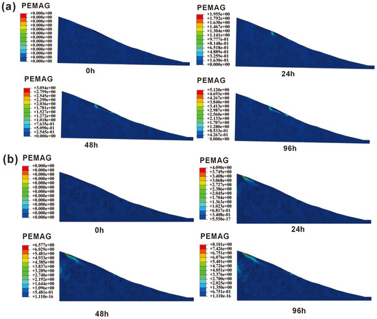
Figure 8.
(a) Plastic distribution contour maps of the GHBL at different time steps under the 50-year return period rainfall condition. (b) Plastic distribution contour maps of the GHBL at different time steps under the 100-year return period rainfall condition.
A comparative analysis of the GHBL under these two rainfall scenarios revealed that when the rainfall peak reached the 100-year return period, the internal stress of the soil mass increased by approximately 1.0 times, displacement increased by approximately 1.5 times, and the plastic zone was significantly larger and more pronounced compared to the 50-year return period scenario. These findings indicated that under the 100-year return period rainfall, the slope exhibited significantly lower stability and a higher risk of failure, providing a basis for further landslide motion simulations. Additionally, the thickness of the sliding mass differed between the two rainfall conditions, with the 50-year return period scenario having yielded a sliding mass thickness of approximately 6 m, while the 100-year return period scenario resulted in a thickness of approximately 8 m. This difference served as an essential reference for the subsequent numerical simulations of slope stability and geological model construction.
4.1.2. Stability Assessment
The factor of safety and failure probability obtained from GeoStudio (Table 5) indicated significant variations in slope stability under different rainfall conditions. Under natural conditions, the stability factor of the GHBL was 1.208, with a failure probability of 12.7%, suggesting a relatively stable slope in its natural state. However, under the 50-year return period rainfall, the stability factor decreased to 0.955, while the failure probability rose sharply to 82.1%, indicating a substantial reduction in slope stability. For the 100-year return period rainfall, the stability factor further decreased to 0.836, and the failure probability increased to 95.7%, suggesting an extremely high likelihood of slope failure under extreme rainfall conditions.
Table 5.
Results of the slope stability and failure probability of the GHBL under three different rainfall scenarios.
These results demonstrated that prolonged rainfall significantly reduced slope stability, leading to higher failure probability and lower reliability index. When the soil mass became saturated, its stability deteriorated considerably, particularly when rainfall-induced groundwater-level rise increased pore water pressure, causing the loosening of the slope. This process weakened the structural integrity of the slope, substantially raising the risk of landslides and other geohazards, thereby posing a serious threat to slope safety.
4.2. Landslide Kinematic Process
Figure 9 and Figure 10 show the simulation results of the GHB landslide using PFC 2D and PFC 3D, respectively. The movement and spatial distribution of the landslide were illustrated under 50-year and 100-year extreme rainfall return periods. The total duration of the landslide was approximately 80 s. Distinct differences in landslide behavior were observed under the two rainfall scenarios. Under the 50-year return period, the maximum velocity of 19.7 m/s was reached at 13.86 s, and the maximum runout distance of 197 m was reached at 75.77 s. Under the 100-year return period, a maximum velocity of 20.6 m/s was reached at 15.6 s, and the maximum runout distance of 280 m was reached at 73.12 s.
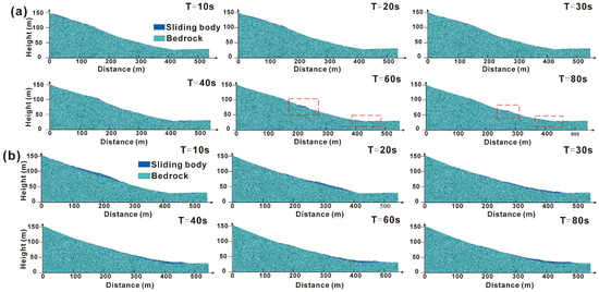
Figure 9.
(a) Two-dimensional kinematic characteristics of the GHBL under the 50-year return period rainfall condition. (b) Two-dimensional kinematic characteristics of the GHBL under the 100-year return period rainfall condition.
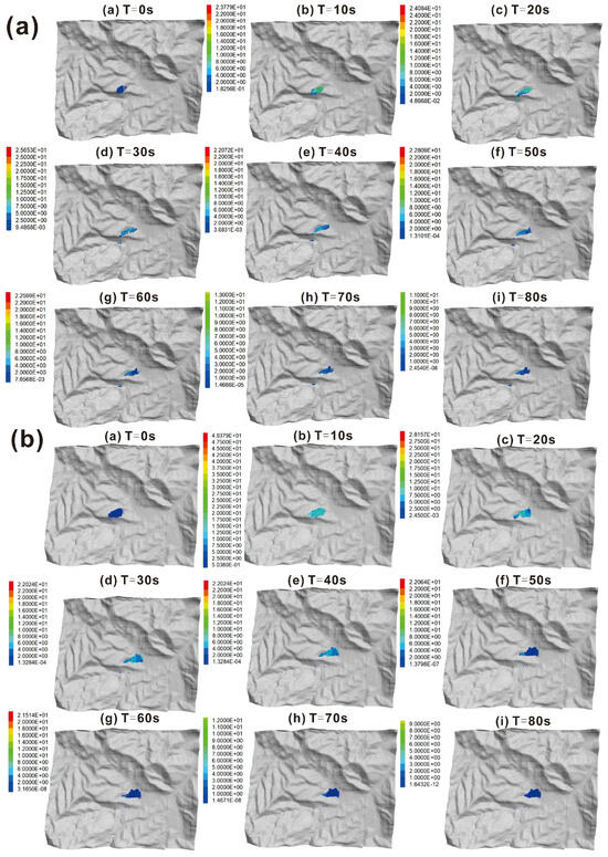
Figure 10.
The 3D landslide kinetics at various moments are shown as follows: (a) rainfall scenario with a 50-year return period, and (b) rainfall scenario with a 100-year return period.
Overall, during the landslide movement, the sliding mass primarily migrated toward lower terrain, following the gully channel. Upon exiting the gully outlet, the terrain became flatter and more open, causing debris to disperse laterally and ultimately form a fan-shaped accumulation in the residential area at the gully outlet. This movement pattern suggested that the extent of landslide flow is influenced by topographic characteristics, where the gully channel constrains the sliding mass, while open terrain promoted debris dispersion and deposition.
4.3. Building Vulnerability
4.3.1. Numerical Simulation of Building Damages
Upon completion of the computation, structural displacement, material stress, and concrete damage contour maps were extracted for building vulnerability analysis. The structural displacement contour map (Figure 11a) indicated that displacement initially increased, followed by a slight rebound, and eventually stabilized at 2.176 mm. During the initial phase of load application, as the load increased, the structural displacement gradually grew. At the 4th minute, when the load reached its peak value, the displacement continued to increase, exhibiting a lag effect, which may have been attributed to damage in structural components leading to a reduction in lateral stiffness. The maximum displacement of 2.7 mm occurred at 6.6 min, primarily at the top of the outermost corner column on the impacted side. Subsequently, as the load gradually decreased, the structural displacement exhibited a rebound, ultimately recovering 0.524 mm, accounting for approximately 1/5 of the total displacement.
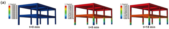
Figure 11.
The ABAQUS simulation results of the two-story building under landslide impact at different moments (0, 8, and 18 min): (a) overall displacement, (b) concrete stress, (c) reinforcement stress, and (d) concrete stiffness degradation.
The concrete Mises stress contour map (Figure 11b) indicated that the maximum stress consistently occurred at the corner column on the impacted side, reaching 2.275 × 10⁷ Pa at the 4th minute. Subsequently, stress gradually decreased and eventually stabilized at 9.774 × 10⁶ Pa, following a trend consistent with the load–time curve. Additionally, significant stress concentrations were observed at the beam–column connections on the non-impacted side, which could be attributed to the rigid beam–column connections that constrained column displacement, leading to localized stress concentration. The reinforcement Mises stress contour map (Figure 11c) indicated that, compared to concrete, the reinforcement experienced higher loads, but the location of maximum stress was like that of the concrete, occurring at the corner column on the impacted side. The maximum stress was recorded at 3.8 min, reaching 2.7 × 10⁸ Pa. Unlike concrete, although the load gradually decreased over time, the reinforcement stress remained around 2.7 × 10⁸ Pa and continued to propagate along the longitudinal reinforcement. This suggested that, at this stage, the reinforcement bore the primary load, while the concrete had already failed. By comparing the stress contour maps of concrete and reinforcement, it was observed that in the primary load-bearing regions (columns), the stress in the reinforcement was approximately ten times that of the concrete. Conversely, in non-impacted areas (beams and slabs), the concrete experienced greater stress than the reinforcement. This indicated that in high-stress regions, concrete underwent a brittle failure due to excessive stress, causing the load to be transferred to the reinforcement after concrete failure. In contrast, in lower-stress areas, the concrete remained intact, resulting in the reinforcement experiencing relatively lower stress levels.
The concrete damage contour map (Figure 11d) indicates that all six perimeter columns exhibited varying degrees of stiffness degradation. On the impacted side, damage primarily occurred on the inner side of the columns, with a continuous expansion trend during the first 4 min. This was attributed to tensile stress in this region, where increasing load led to failure of the concrete cover, causing reinforcement deformation and further exacerbating tensile zone deformation. Between 4 and 18 min, the damage expansion rate slowed, with only a slight increase along the tensile side of the concrete, as the failed concrete transferred more deformation to the reinforcement, resulting in continued expansion of the damaged area. This trend aligned with the reinforcement stress contour map, further confirming concrete failure. On the non-impacted side, damage was primarily concentrated at the column bases and beam–column connections at the top, where high-constraint conditions led to stress concentration, predominantly occurring in the tensile regions of the concrete, consistent with actual structural behavior. Finally, by quantifying the number of damaged mesh elements in the concrete and calculating their ratio to the total mesh elements of the building, the vulnerability of the two-story building was determined to be 0.28.
4.3.2. Building Vulnerability Mapping
The abovementioned simulation was carried out on each building within the impact area of the landslide to determine its vulnerability values. The results were then integrated within GIS, generating a building vulnerability distribution map.
According to the statistical results in Figure 12 under different rainfall conditions, the number of low-, medium-, and high-vulnerability buildings under the 50-year return period rainfall condition was 3, 5, and 6, respectively, while under the 100-year return period rainfall condition, the corresponding numbers were 4, 7, and 9. It was evident that as rainfall intensity increased, the number of medium- and high-vulnerability buildings increased by 2 and 3, respectively. Analysis of the building vulnerability distribution map in Figure 13 further revealed that under the 50-year return period rainfall, the building vulnerability values decreased from 0.87 to 0, while under the 100-year return period rainfall, the values decreased from 1 to 0. This indicated that under a single rainfall scenario, building vulnerability exhibited a distinct spatial gradient pattern, primarily controlled by the relative distance between buildings and the landslide slip surface or slope toe. As this spatial distance increased, the impact force of the landslide gradually attenuated, reducing the mechanical loads acting on buildings, which ultimately resulted in a progressive decline in vulnerability values from the landslide frontal edge (high-vulnerability zone) to the periphery of the affected area.
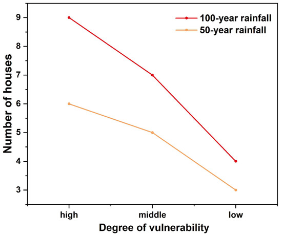
Figure 12.
Number of houses with different damage levels under different working conditions.
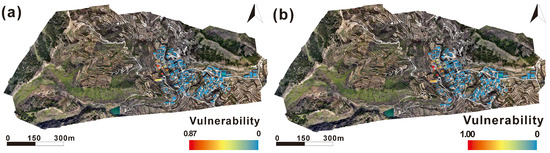
Figure 13.
(a) Building vulnerability map under the 50-year return period rainfall scenario. (b) Building vulnerability map under the 100-year return period rainfall scenario.
A comparative analysis of different rainfall scenarios demonstrated that the maximum building vulnerability increased from 0.87 to 1, while the increase in medium- and high-vulnerability buildings further confirmed the significant influence of rainfall parameters on landslide dynamics. The increase in rainfall intensity notably enhanced groundwater infiltration rates, thereby reducing the shear strength of the sliding zone soil and expanding the landslide’s affected area. Additionally, the rapid rise in pore water pressure induced by intense rainfall accelerated landslide motion, increasing the kinetic energy of the sliding mass, which in turn elevated the probability of building impact damage.
In the visualization results, the expansion of dark-colored areas and the deepening of color intensity directly reflected the spatial propagation of high-vulnerability zones, indicating that under extreme rainfall conditions, both the extent and severity of building damage significantly increased. Notably, the number and distribution of blue-colored buildings remained relatively unchanged across different rainfall conditions, suggesting that the impact of landslides on these buildings under rainfall scenarios was relatively low, posing minimal hazard.
5. Discussion
In this section, we will analyze and compare current results in the context of the existing literature, discuss their limitations, and outline directions for future studies.
Previous studies focused on predicting landslide occurrence using empirical or statistical methods [57,58]. For example, Segoni et al. established rainfall thresholds for landslide initiation based on historical data; however, their approach did not consider post-failure dynamics or the vulnerability of affected buildings [19]. In contrast, our study not only predicts landslide occurrence under extreme rainfall scenarios (with 50-year and 100-year return periods corresponding to 184.6 mm and 209.3 mm of rainfall, respectively), but also simulates the entire process from slope failure to building impact, thereby offering a more comprehensive assessment of the results. Through coupled seepage–stress analysis using ABAQUS, we found that under the 100-year rainfall scenario, the plastic zone expanded by 58% compared to the 50-year scenario (with the maximum plastic strain increasing from 5.12 to 8.10). This directly links rainfall intensity to slope instability. These findings are consistent with the work of Guo et al., who emphasized the role of pore water pressure in slope failure [10]; however, our study further quantifies the spatial extent of plastic deformation, providing more precise information for stability analysis and hazard zonation.
Existing vulnerability assessments often rely on qualitative indicators or empirical fragility curves [59,60]. For instance, Singh et al. proposed a semi-quantitative method based on building typology and landslide intensity, but their approach lacked insight into the structural damage mechanisms [25]. In contrast, our study employed the Concrete Damaged Plasticity (CDP) model in ABAQUS to simulate concrete stiffness degradation and steel-reinforcement yielding under dynamic loading. The results show that when the rainfall intensity increases from a 50-year to a 100-year return period, the vulnerability of a two-story reinforced concrete building rises from 0.28 to 0.43. This mechanistic approach addresses a key limitation of data-driven methods, which often overlook the nonlinear behavior of materials under impact loading [27]. For example, our simulation revealed that the stress in the steel reinforcement of load-bearing columns (2.7 × 10⁸ Pa) is an order of magnitude higher than that in the surrounding concrete (2.7 × 10⁷ Pa), highlighting the importance of considering material-specific failure modes in vulnerability assessments.
The role of extreme rainfall in slope instability has been well documented [61,62]; however, few studies have quantified its impact on building vulnerability. Our PFC simulations show that, compared to the 50-year rainfall scenario, the 100-year scenario results in a 4.6% increase in landslide velocity (from 19.7 m/s to 20.6 m/s) and a 42% increase in distance runout (from 197 m to 280 m). These findings are consistent with the work of Hu et al., who observed similar velocity amplification in debris flows [7]. However, our study uniquely links such dynamic changes to building damage through vulnerability mapping (Figure 13). Importantly, our analysis of historical rainfall data (1980–2017) reveals that in extreme years—such as July 2015—a single three-day rainfall event accounted for up to 79% of the annual precipitation. This highlights the necessity of considering temporal resolution in rainfall analysis, as short-duration extreme events may trigger landslides more abruptly than monthly cumulative rainfall totals.
Naturally, our study is subject to several limitations and potential sources of error. First, there is uncertainty in input parameters, especially the saturated permeability and the soil-water characteristic curve. As Komolvilas et al. reported, permeability in similar soils can vary by up to 50%, which may significantly alter seepage patterns [11]. Field measures could reduce this uncertainty, but such measures are not possible in some cases due to sparse data and the fact that they are time-consuming. To quantify such uncertainties, it may be useful to perform Monte Carlo analysis and add confidence intervals to vulnerability maps. However, we note that various numerical simulation methods were integrated in our analysis, and all of them were associated with parameter uncertainty. This means that some intermediate steps transferred their uncertainties to the next step, and the impacts from the last step might be nonlinear. Hence, it is really difficult to quantify and integrate all of these uncertainties into the final results of the building vulnerability. Additionally, the Mohr–Coulomb model assumes homogeneous strength, whereas real-world slopes commonly exhibit heterogeneous behavior [63]. This may explain why the simulated failure zones appear slightly narrower than observed (Figure 8). The PFC simulations also involve inherent simplifications. The use of particles ranging from 0.4 to 0.7 m in diameter (Table 3) oversimplifies interparticle interactions and may underestimate the degree of fragmentation. Calhoun and Clague [64] highlighted that smaller particles (<0.1 m) dominate fluid flow in natural landslides. Hence, it can be expected that our predicted runout distances might be conservative, since the liquidity of bigger particles was inevitably worse. Furthermore, the model does not account for bedrock fractures or weak interlayers, which are known to act as preferential flow paths [46]. Including these features could improve the accuracy of the kinematic simulations. Regarding the rainfall scenario analysis, the extreme values were determined based on the stationary assumption: the used rainfall series and its statistical properties were invariant versus time. However, it is well-known that climate change has been leading to extensive rainfall changes for decades [65,66]. Moreover, the absence of rainfall records after 2017 may fail to capture recent climate extremes. For example, a rainstorm (>250 mm over three days) occurred in Tianjin City in 2022, and it was not taken into account in our analysis due to data availability. This may result in an underestimation of the true threshold for extreme rainfall. Hence, nonstationary rainfall time series and dynamic parameters for Gumbel distribution should be involved in future analyses and predictions.
While the use of GeoStudio for slope stability analysis offers high computational efficiency, its inherent simplification of complex three-dimensional geological conditions into a two-dimensional framework introduces a critical limitation. Previous studies have shown that in narrow gullies or ridge terrains, 2D analyses may overestimate the factor of safety by 10–20% due to the dominant influence of 3D confinement effects [41]. In the present case, the GHBL landslide exhibits a narrow and elongated morphology (approximately 420 m in length and 130 m in width). The shear resistance along the lateral margins of the landslide mass is significantly influenced by sidewall friction. Therefore, the 2D simplification likely introduces deviations in the stability evaluation for such geometrically constrained terrain. We notice that the reasons for the wide usage of 2D models’ issues are mainly associated with data availability and the complexity of 3D modeling. In addition, applicable conditions of numerical models and actual contexts of the cases are also constraints [21]. Hence, a technique for 3D modeling which incorporates the impact of subsurface heterogeneity on seepage and stability may be of high interest.
In future work, we will focus on the following aspects to enhance the robustness and applicability of our model. First, we plan to integrate the Gumbel distribution with regional climate models (RCMs) to project future extreme rainfall under climate change scenarios, as Myhre et al. [5] suggest that the frequency of 100-year rainfall events may increase by up to 30% by 2050, highlighting the need for dynamic threshold updates. Second, we will deploy drone-based hyperspectral sensors to produce high-resolution (<1 m) soil moisture maps, addressing the spatial variability currently overlooked in our model [13]. Third, we intend to incorporate the material point method (MPM) with large deformation contact algorithms to simulate the fully coupled process from slope instability to building impact, especially under complex geological conditions, such as jointed rock masses and weak interlayers. Moreover, it is necessary to conduct lab-impact tests to validate the proposed numerical model. In the current analysis, the option to conduct lab-impact tests was not available due to limited budgets. Finally, we aim to construct a fragility function database for multiple building types based on a representative inventory that accounts for variations in construction materials, building age, and design codes, thereby improving the model’s applicability at the urban scale.
6. Conclusions
This study proposed a quantitative vulnerability assessment method of structures exposed to landslides. A slow-moving landslide in Northern China was taken as an example to test its effectiveness. By statistically analyzing the extreme rainfall for 50-year and 100-year return periods and simulating the landslide-affected area and dynamic characteristics, vulnerability distribution maps of buildings under different rainfall scenarios were obtained. The results indicated that building vulnerability within the landslide-affected area exhibited a significant spatial gradient attenuation pattern. The vulnerability was jointly controlled by the relative distance from the landslide center and dynamic parameters. As the landslide impact force attenuated with increasing distance, building vulnerability decreased progressively from the landslide frontal zone toward the periphery. Compared to the 50-year rainfall scenario, the landslide-affected area under the 100-year rainfall scenario expanded by 10%. The vulnerability of individual buildings raised by 10–15%, with the maximum vulnerability increasing from 0.83 to 1. These findings suggested that under extreme rainfall conditions, landslide intensity intensified significantly, thus substantially increasing the damages of buildings.
Overall, the proposed method was possible to quantitatively predict the damage of buildings, even when landslide hazards have not yet occurred. This study presented a representative case for the quantitative evaluation of building vulnerability caused by rainfall-triggered landslides and provided a scientific foundation for local governments to develop disaster-prevention and -mitigation strategies. Furthermore, future research should focus on regular updates and dynamic monitoring to enhance the accuracy and effectiveness of landslide risk management.
Author Contributions
Conceptualization, G.L., D.L., and M.R.; methodology, G.L., Y.Z., and Z.G.; software, G.L., Y.Z., and J.H.; validation, Y.Z., J.H., H.W., and M.C.; formal analysis, G.L., D.L., M.R., H.W., and M.C; investigation, G.L., D.L., M.R., H.W., and M.C.; resources, G.L. and Y.Z.; data curation, G.L., Y.Z., and J.H.; writing—original draft preparation, G.L., Y.Z., and Z.G.; writing—review and editing, Y.Z., Z.G., and J.H.; visualization, D.L. and Y.Z.; supervision, Z.G.; project administration, H.W. and M.C.; funding acquisition, G.L. and Z.G. All authors have read and agreed to the published version of the manuscript.
Funding
This research was funded by National Natural Science Foundation of China (No. 42307248), and the Planning and Natural Resources Research Project of Tianjin City (2022-40, KJ [2024]25).
Data Availability Statement
The original contributions presented in the study are included in the article, further inquiries can be directed toward the corresponding author.
Conflicts of Interest
Authors Guangming Li and Zizheng Guo was employed by the company Tianjin Municipal Engineering Design & Research Institute (TMEDI) Co., Ltd. Author Dong Liu was employed by the company 11th Geological Brigade of Zhejiang Province. Author Mengjiao Ruan was employed by the company Zhejiang Geology and Mineral Technology Co., Ltd. The remaining authors declare that the research was conducted in the absence of any commercial or financial relationships that could be construed as a potential conflict of interest.
References
- Li, Y.; Yang, X.; Hu, X.; Wan, L.; Ma, E. Mechanisms of rainfall-induced landslides and interception dynamic response: A case study of the Ni changgou landslide in Shimian, China. Sci. Rep. 2024, 14, 1567. [Google Scholar] [CrossRef] [PubMed]
- Amarasinghe, M.P.; Kulathilaka, S.A.S.; Robert, D.J.; Zhou, A.; Jayathissa, H.A.G. Risk assessment and management of rainfall-induced landslides in tropical regions: A review. Nat. Hazards 2024, 120, 2179–2231. [Google Scholar] [CrossRef]
- Fan, L.; Lehmann, P.; Zheng, C.; Or, D. Rainfall intensity temporal patterns affect shallow landslide triggering and hazard evolution. Geophys. Res. Lett. 2020, 47, 994. [Google Scholar] [CrossRef]
- Hürlimann, M.; Guo, Z.; Puig-Polo, C.; Medina, V. Impacts of future climate and land cover changes on landslide susceptibility: Regional scale modelling in the Val d’Aran region (Pyrenees, Spain). Landslides 2022, 19, 99–118. [Google Scholar] [CrossRef]
- Myhre, G.; Alterskjær, K.; Stjern, C.W.; Hodnebrog, H.; Marelle, L.; Samset, B.H.; Stohl, A. Frequency of extreme precipitation increases extensively with event rareness under global warming. Sci. Rep. 2019, 9, 16063. [Google Scholar] [CrossRef]
- Huang, F.; Teng, Z.; Guo, Z.; Catani, F.; Huang, J. Uncertainties of landslide susceptibility prediction: Influences of different spatial resolutions, machine learning models and proportions of training and testing dataset. Rock Mech. Bull. 2023, 2, 100028. [Google Scholar] [CrossRef]
- Liu, L.; Gao, C.; Zhu, Z.; Zhang, S.; Tang, X. Spatiotemporal evolution patterns and underlying formation mechanisms of monsoon rainfall across eastern China: A complex network perspective. Atmos. Res. 2024, 304, 107363. [Google Scholar] [CrossRef]
- Long, X.; Hu, Y.; Gan Bin Zhou, J. Numerical simulation of the mass movement process of the 2018 Sedongpu glacial debris flow by using the fluid-solid coupling method. J. Earth Sci. 2024, 35, 583–596. [Google Scholar] [CrossRef]
- EMDAT, CRED/UCLouvain. Brussels, Belgium. Available online: www.emdat.be (accessed on 15 March 2025).
- Guo, Z.; Chen, L.; Yin, K.; Shrestha, D.P.; Zhang, L. Quantitative risk assessment of slow-moving landslides from the viewpoint of decision-making: A case study of the Three Gorges Reservoir in China. Eng. Geol. 2020, 273, 105667. [Google Scholar] [CrossRef]
- Komolvilas, V.; Tanapalungkorn, W.; Latcharote, P.; Likitlersuang, S. Failure analysis on a heavy rainfall-induced landslide in Huay Khab Mountain in Northern Thailand. J. Mt. Sci. 2021, 18, 2580–2596. [Google Scholar] [CrossRef]
- Long, Y.; Li, W.; Huang, R.; Xu, Q.; Yu, B.; Liu, G. A Comparative study of supervised classification methods for investigating landslide evolution in the Mianyuan River basin, China. J. Earth Sci. 2023, 34, 316–329. [Google Scholar] [CrossRef]
- Guo, Z.; Wang, H.; He, J.; Huang, D.; Song, Y.; Wang, T.; Liu, Y.; Ferrer, J.V. PSLSA v2.0: An automatic Python package integrating machine learning models for regional landslide susceptibility assessment. Environ. Model. Softw. 2025, 186, 106367. [Google Scholar] [CrossRef]
- Zhang, L.; Wu, F.; Wei, X.; Yang, H.; Fu, S.; Huang, J.; Gao, L. Polynomial chaos surrogate and bayesian learning for coupled hydro-mechanical behavior of soil slope. Rock Mech. Bull. 2023, 2, 100023. [Google Scholar] [CrossRef]
- Li, K.; Sun, P.; Wang, H.; Ren, J. Insight into failure mechanisms of rainfall induced mudstone landslide controlled by structural planes: From laboratory experiments. Eng. Geol. 2024, 343, 107774. [Google Scholar] [CrossRef]
- Zhang, C.; Zhang, M.; Zhang, T.; Dai, Z.; Wang, L. Influence of intrusive granite dyke on rainfall-induced soil slope failure. Bull. Eng. Geol. Environ. 2020, 79, 5259–5276. [Google Scholar] [CrossRef]
- Liu, X.; Wang, Y.; Li, D.Q. Numerical simulation of the 1995 rainfall-induced Fei Tsui Road landslide in Hong Kong: New insights from hydro-mechanically coupled material point method. Landslides 2020, 17, 2755–2775. [Google Scholar] [CrossRef]
- Li, W.; Huang, Y. Model tests on the effect of dip angles on flow behavior of liquefied sand. J. Earth Sci. 2023, 34, 381–385. [Google Scholar] [CrossRef]
- Segoni, S.; Piciullo, L.; Gariano, S.L. A review of the recent literature on rainfall thresholds for landslide occurrence. Landslides 2018, 15, 1483–1501. [Google Scholar] [CrossRef]
- Li, G.; Zhang, Y.; Zhang, Y.; Guo, Z.; Liu, Y.; Zhou, X.; Guo, Z.; Guo, W.; Wan, L.; Duan, L.; et al. Landslide hazard prediction based on UAV remote sensing and discrete element model simulation—Case from the Zhuangguoyu landslide in Northern China. Remote Sens. 2024, 16, 3887. [Google Scholar] [CrossRef]
- Guo, Z.; Zhou, X.; Huang, D.; Zhai, S.; Tian, B. Dynamic simulation insights into friction weakening effect on rapid long-runout landslides: A case study of the Yigong landslide in the Tibetan Plateau, China. China Geol. 2024, 7, 222–236. [Google Scholar] [CrossRef]
- Guo, L.; Chen, G.; Ding, L.; Zheng, L.; Gao, J. Numerical simulation of full desiccation process of clayey soils using an extended DDA model with soil suction consideration. Comput. Geotech. 2023, 153, 105107. [Google Scholar] [CrossRef]
- Yang, Y.; Li, J.; Shi, W.; Yang, C.; Yan, L. Numerical investigation of failure characteristics debris movement in the Madaling landslide using coupled, FDM–DEM. Geotech. Geol. Eng. 2024, 42, 2745–2765. [Google Scholar] [CrossRef]
- Liu, X.; Wang, Y. Probabilistic simulation of entire process of rainfall-induced landslides using random finite element and material point methods with hydro-mechanical coupling. Comput. Geotech. 2021, 132, 103989. [Google Scholar] [CrossRef]
- Singh, A.; Kanungo, D.P.; Pal, S. A modified approach for semi-quantitative estimation of physical vulnerability of buildings exposed to different landslide intensity scenarios. Georisk Assess. Manag. Risk Eng. Syst. Geohazards 2019, 13, 66–81. [Google Scholar] [CrossRef]
- Medina, V.; Hürlimann, M.; Guo, Z.; Lloret, A.; Vaunat, J. Fast physically-based model for rainfall-induced landslide susceptibility assessment at regional scale. Catena 2021, 201, 105213. [Google Scholar] [CrossRef]
- Luo, H.Y.; Zhang, L.M.; Zhang, L.L.; He, J.; Yin, K.S. Vulnerability of buildings to landslides: The state of the art and future needs. Earth Sci. Rev. 2023, 238, 104329. [Google Scholar] [CrossRef]
- Luo, H.Y.; Fan, R.L.; Wang, H.J.; Zhang, L.M. Physics of building vulnerability to debris flows, floods and earth flows. Eng. Geol. 2020, 271, 105611. [Google Scholar] [CrossRef]
- Chen, Q.; Chen, L.; Gui, L.; Yin, K.; Shrestha, D.P.; Du, J.; Cao, X. Assessment of the physical vulnerability of buildings affected by slow-moving landslides. Nat. Hazards Earth Syst. Sci. 2020, 20, 2547–2565. [Google Scholar] [CrossRef]
- Yin, D.B.; Zheng, Q.; Zhou, A.; Shen, S.L. Enhancing landslide hazard prevention: Mapping vulnerability via considering the effects of human factors. Int. J. Disaster Risk Reduct. 2024, 108, 104509. [Google Scholar] [CrossRef]
- Wang, T.; Yin, K.; Li, Y.; Chen, L.; Xiao, C.; Zhu, H.; Westen, C.V. Physical vulnerability curve construction and quantitative risk assessment of a typhoon-triggered debris flow via numerical simulation: A case study of Zhejiang Province, SE China. Landslides 2024, 21, 1333–1352. [Google Scholar] [CrossRef]
- Bakalis, K.; Vamvatsikos, D. Seismic fragility functions via nonlinear response history analysis. J. Struct. Eng. 2018, 144, 04018181. [Google Scholar] [CrossRef]
- Zhang, Z.; Feng, F.; Wang, T.; Dou, X. Numerical estimation of landslide runout flow–structure interactions: A case study of Zhengjiamo landslide. Bull. Eng. Geol. Environ. 2024, 83, 212. [Google Scholar] [CrossRef]
- Xing, L.; Wang, G.; Gong, W.; Xu, M.; Jaboyedoff, M.; Wang, F. Model tests of the failure behaviors of buildings under the impact of granular flow. Landslides 2025, 22, 373–392. [Google Scholar] [CrossRef]
- Wang, X.; Yin, J.; Luo, M.; Ren, H.; Li, J.; Wang, L.; Li, D.; Li, G. Active High-Locality Landslides in Mao County: Early Identification and Deformational Rules. J. Earth Sci. 2023, 34, 1596–1615. [Google Scholar] [CrossRef]
- Montes-Pajuelo, R.; Rodríguez-Pérez, Á.M.; López, R.; Rodríguez, C.A. Analysis of probability distributions for modelling extreme rainfall events and detecting climate change: Insights from mathematical and statistical methods. Mathematics 2024, 12, 1093. [Google Scholar] [CrossRef]
- Back, Á.J.; Bonfante, F.M. Evaluation of generalized extreme value and Gumbel distributions for estimating maximum daily rainfall. Rev. Bras. Cienc. Ambient. 2021, 56, 654–664. [Google Scholar] [CrossRef]
- Gnyawali, K.; Dahal, K.; Talchabhadel, R.; Nirandjan, S. Framework for rainfall-triggered landslide-prone critical infrastructure zonation. Sci. Total Environ. 2023, 872, 162242. [Google Scholar] [CrossRef]
- Dassault Systèmes. ABAQUS Analysis User’s Manual, Version 2022; Dassault Systèmes: Providence, RI, USA, 2022; pp. 800–950. [Google Scholar]
- Ortiz-Giraldo, L.; Botero, B.A.; Vega, J. An integral assessment of landslide dams generated by the occurrence of rainfall-induced landslide and debris flow hazard chain. Front. Earth Sci. 2023, 11, 1157881. [Google Scholar] [CrossRef]
- Xiao, L.; Wang, J.; Zhu, Y.; Zhang, J. Quantitative risk analysis of a rainfall-induced complex landslide in Wanzhou county, three gorges reservoir, China. Int. J. Disaster Risk Sci. 2020, 11, 347–363. [Google Scholar] [CrossRef]
- Świtała, B.M. Numerical simulations of triaxial tests on soil-root composites and extension to practical problem: Rainfall-induced landslide. Int. J. Geomech. 2020, 20, 04020206. [Google Scholar] [CrossRef]
- Liang, C.; Wu, Z.; Liu, X.; Xiong, Z.; Li, T. Analysis of shallow landslide mechanism of expansive soil slope under rainfall: A case study. Arab. J. Geosci. 2021, 14, 584. [Google Scholar] [CrossRef]
- Paswan, A.P.; Shrivastava, A.K. Modelling of rainfall-induced landslide: A threshold-based approach. Arab. J. Geosci. 2022, 15, 795. [Google Scholar] [CrossRef]
- Shoaib, M.; Yang, W.; Liang, Y.; Rehman, G. Stability and deformation analysis of landslide under coupling effect of rainfall and reservoir drawdown. Civ. Eng. J. 2021, 7, 1098–1111. [Google Scholar] [CrossRef]
- Wei, L.; Cheng, H.; Dai, Z. Propagation modeling of rainfall-induced landslides: A case study of the Shaziba Landslide in Enshi, China. Water 2023, 15, 424. [Google Scholar] [CrossRef]
- Mao, W.; Li, W.; Rouzbeh, R.; Naveed, A.; Zheng, H.; Huang, Y. Numerical Simulation of Liquefaction-Induced Settlement of Existing Structures. J. Earth Sci. 2023, 34, 339–346. [Google Scholar] [CrossRef]
- Távara, L.; Moreno, L.; Paloma, E.; Mantič, V. Accurate modelling of instabilities caused by multi-site interface-crack onset and propagation in composites using the sequentially linear analysis and Abaqus. Compos. Struct. 2019, 225, 110993. [Google Scholar] [CrossRef]
- Hu, X.; Zhang, L.; Hu, K.; Cui, L.; Wang, L.; Xia, Z.; Huang, Q. Modelling the evolution of propagation and runout from a gravel–silty clay landslide to a debris flow in Shaziba, southwestern Hubei Province, China. Landslides 2022, 19, 2199–2212. [Google Scholar] [CrossRef]
- Xie, Q.; Cao, Z.; Sun, W.; Fumagalli, A.; Fu, X.; Wu, Z.; Wu, K. Numerical simulation of the fluid-solid coupling mechanism of water and mud inrush in a water-rich fault tunnel. Tunn. Undergr. Space Technol. 2023, 131, 104796. [Google Scholar] [CrossRef]
- Li, S.; Qiu, C.; Huang, J.; Guo, X.; Hu, Y.; Mugahed, A.S.Q.; Tan, J. Stability analysis of a high-steep dump slope under different rainfall conditions. Sustainability 2022, 14, 11148. [Google Scholar] [CrossRef]
- Minh, H.L.; Khatir, S.; Wahab, M.A.; Cuong-Le, T. A concrete damage plasticity model for predicting the effects of compressive high-strength concrete under static and dynamic loads. J. Build. Eng. 2021, 44, 103239. [Google Scholar] [CrossRef]
- Luan, T.M.; Khatir, S.; Cuong-Le, T. Concrete Damage Plastic Model for High Strength-Concrete: Applications in Reinforced Concrete Slab and CFT Columns. Iran J. Sci. Technol. Trans. Civ. Eng. 2024, 1–20. [Google Scholar] [CrossRef]
- Lee, S.H.; Abolmaali, A.; Shin, K.J.; Lee, H.D. ABAQUS modeling for post-tensioned reinforced concrete beams. J. Build. Eng. 2020, 30, 101273. [Google Scholar] [CrossRef]
- Nagy, N.; Mohamed, M.; Boot, J.C. Nonlinear numerical modelling for the effects of surface explosions on buried reinforced concrete structures. Geomech. Eng. 2010, 2, 1–18. [Google Scholar] [CrossRef]
- Tao, Z.; Wang, Z.B.; Yu, Q. Finite element modelling of concrete-filled steel stub columns under axial compression. J. Constr. Steel Res. 2013, 89, 121–131. [Google Scholar] [CrossRef]
- Du, B.; Wang, Y.; Fang, Z.; Liu, G.; Tian, Z. Spatiotemporal modeling and projection framework of rainfall-induced landslide risk under climate change. J. Environ. Manag. 2025, 373, 123474. [Google Scholar] [CrossRef]
- Fang, Z.; Wang, J.; Wang, Y.; Du, B.; Liu, G. Improved landslide prediction by considering continuous and discrete spatial dependency. Landslides 2025, 22, 1107–1122. [Google Scholar] [CrossRef]
- Emkani, M.; Yazdi, M.; Zarei, E.; Klockner, K.; Alimohammadlou, M.; Kamalinia, M. Advancing understanding of vulnerability assessment in process industries: A systematic review of methods and approaches. Int. J. Disaster Risk Reduc. 2024, 107, 104479. [Google Scholar] [CrossRef]
- Diaz-Sarachaga, J.M.; Jato-Espino, D. Analysis of vulnerability assessment frameworks and methodologies in urban areas. Nat. Hazards 2020, 100, 437–457. [Google Scholar] [CrossRef]
- Tao, H.; Zhang, M.; Gong, L.; Shi, X.; Wang, Y.; Yang, G.; Lei, S. The mechanism of slope instability due to rainfall-induced structural decay of earthquake-damaged loess. Earthq. Res. Adv. 2022, 2, 100137. [Google Scholar] [CrossRef]
- Liang, C.; Wu, S. Centrifuge modeling of intact clayey loess slope by rainfall. Environ. Earth Sci. 2024, 83, 352. [Google Scholar] [CrossRef]
- Xiang, X.; Zi-Hang, D. Numerical implementation of a modified Mohr–Coulomb model and its application in slope stability analysis. J. Mod. Transp. 2017, 25, 40–51. [Google Scholar] [CrossRef]
- Calhoun, N.C.; Clague, J.J. Distinguishing between debris flows and hyperconcentrated flows: An example from the eastern Swiss Alps. Earth Surf. Process. Landf. 2018, 43, 1280–1294. [Google Scholar] [CrossRef]
- Gariano, S.L.; Guzzetti, F. Landslides in a changing climate. Earth-Sci. Rev. 2016, 162, 227–252. [Google Scholar] [CrossRef]
- Guo, Z.; Ferrer, J.V.; Hürlimann, M.; Medina, V.; Puig-Polo, C.; Yin, K.; Huang, D. Shallow landslide susceptibility assessment under future climate and land cover changes: A case study from southwest China. Geosci. Front. 2023, 14, 101542. [Google Scholar] [CrossRef]
Disclaimer/Publisher’s Note: The statements, opinions and data contained in all publications are solely those of the individual author(s) and contributor(s) and not of MDPI and/or the editor(s). MDPI and/or the editor(s) disclaim responsibility for any injury to people or property resulting from any ideas, methods, instructions or products referred to in the content. |
© 2025 by the authors. Licensee MDPI, Basel, Switzerland. This article is an open access article distributed under the terms and conditions of the Creative Commons Attribution (CC BY) license (https://creativecommons.org/licenses/by/4.0/).