Numerical Validation of Fully Coupled Nonlinear Seismic Soil–Pile–Structure Interaction

Abstract

While many researchers have broadly studied soil–structure interaction (SSI) problems to comprehend SSI effects on the overall system’s behavior, some critical numerical modeling issues have not been sufficiently investigated to achieve the most accurate results. Furthermore, most scholars have not provided detailed explanations of the validation process for their proposed numerical models. Modeling pile foundations in a three-dimensional (3D) continuum system in a fully coupled manner is often challenging for engineers who do not specialize in structural and geotechnical earthquake engineering, as it can be very time-consuming and complicated. Therefore, this work aims to validate a finite element model of seismic soil–pile–structure interaction (SPSI) problems in a continuum soil body by comparing the results of numerical models with those of a centrifuge test and computed numerical simulations available in the literature. In this regard, several newly developed elements in OpenSees (Version 3.6.0) are tested. The results of this work demonstrate a closer alignment with prior experimental research findings. It is believed that providing detailed numerical modeling and validation processes will assist researchers in better understanding crucial issues in modeling soil–pile–structure interaction problems.

1. Introduction

The behavior of piles under seismic loading is a critical factor that may significantly impact the overall system’s (soil–pile–structure) performance. Therefore, many researchers have studied soil–pile–structure interaction (SPSI) problems extensively for decades [1,2,3,4,5,6]. In general, SPSI problems can be solved by analytical, numerical, and experimental methods. While reaching a solution using analytical techniques is very challenging for complex SPSI problems, experimental methods can be economically costly and too time consuming to set up the real test environment. Thus, numerical methods stand out from these two methods for offering reliable solutions because of the following reasons. (1) Complicated problems can be solved using advanced computer technology, (2) which is cheaper than experimental research, and (3) it is more practical for designers to set up a model in virtual environments. In addition, especially in geotechnical earthquake engineering (GEE), calculations have recently become substantially more accurate and efficient due to the rapid advancement of computing technology [7].

Numerous numerical methods, such as the finite element method (FEM), finite difference method (FDM), boundary element method (BEM), discrete element method (DEM), finite volume method (FVM), extended finite element method (X-FEM), discontinuous deformation method (DDM), finite cover method (FCM), peridynamics (PD), smoothed particle hydrodynamics (SPH), and material point method (MPM), have been widely used in the GEE. Among all, FEM is one of the most adopted approaches since it allows for high computing efficiency; that is, it is very versatile for various problems of engineering and mathematical physics. It is also capable of reproducing failures of specimens or experiments in a laboratory and massive geotechnical structures in the field [8]. Therefore, in the late 1990s and early 2000s, the FEM software industry had grown into a multibillion-dollar market. Several well-known FEM software companies included LS-DYNA, ABAQUS, ANSYS, NASTRAN, ADINA, CSI, and COMSOL Multiphysics. In addition, currently, there is an abundance of open-source FEM software accessible online, including Elmer, FreeFEM, FeniCS Project, FEBio, DUNE, and Open System for Earthquake Engineering Simulation (OpenSees) [9]. From a range of numerical analysis software, the finite element program, OpenSees, created by McKenna and Fenves [10], has several advantages to carrying out numerical analyses using FEM, which can be expressed as follows: (1) an open-source software, (2) a very active community that continuously improves the content, (3) being used by many researchers for scientific studies, so many libraries were already validated, (4) the capability of implementing constitutive models, solution methods, and data processing and communication procedures using object-oriented methodologies to maximize versatility, and so on.

Many scholars have used OpenSees for years to approximate a solution to different SPSI problems [11,12,13,14,15,16,17]. In addition, several have validated SPSI results either via centrifuge, shaking table, or various field tests [18,19,20,21,22,23,24,25,26]. Based on the majority of referenced research, a continuum model must be constructed using a direct approach to incorporate all components of SPSI effects, which include (1) kinematic interaction, (2) inertial interaction, and (3) subgrade impedances with a fully coupled (u–P formulation) system. However, many designers refrain from performing SPSI analyses using a continuum model because they can be very time consuming. It is also challenging to add many contact and interaction elements during the setup of complex problems. In addition, designers have to deal with numerous geotechnical parameters that are complex and incomprehensible to structural engineers. This is why employing Beam on Nonlinear Winkler Foundation (BNWF) models is considered more practical, although the system’s response can be under- or overestimated.

Until the 2020s, solving complex SPSI problems in a continuum using the OpenSees library’s elements was extremely challenging. In particular, the construction of absorbing boundaries, even if it was possible to create them, did not yield completely accurate results. Also, contact elements and meshing issues made it more difficult for a continuum model to converge to the solution. Recently, several elements have been included in the OpenSees library by ASDEA Software Technology to tackle these shortcomings. These are ASDEmbeddedNodeElement, zeroLengthContactASDimplex, and ASDAbsorbingBoundary, and further details for the elements will be provided in forthcoming sections. ASDEA Software Technology also has a graphic user interface (GUI) named Scientific Toolkit for OpenSees (STKO Version 3.3.0) [27], which assists in creating complex models during pre-processing, and in visualizing results for post-processing whenever needed. Since the elements mentioned above are relatively recent improvements to the OpenSees library, they have not yet been implemented and tested for various problems; thus, necessary validations are critically needed, particularly for SPSI problems.

Therefore, this work aims to validate newly developed contact and absorbing boundary elements in OpenSees (Version 3.6.0) via a centrifuge test. Although developers perform preliminary checks of these elements, the benchmark problems used remain relatively simple compared to real-world problems exposed to seismic excitations. In addition, to the best of the authors’ knowledge, these elements have not been utilized for any SPSI problems in the literature yet. Consequently, we simulated a centrifuge experiment that represents a fundamental real-world example. By simulating a centrifuge experiment representative of practical scenarios, we seek to fill this gap in knowledge and provide valuable insights for researchers aiming to utilize these elements in their modeling endeavors. It is worth mentioning that since this work solely focuses on validating and providing exclusive information on these elements, we do not elaborate on soil, pile, and structure response independently. It is believed that the findings will provide baseline data in the literature to encourage researchers to employ more practical contact and absorbing elements in modeling SPSI problems in OpenSees.

The remaining sections of the paper are structured as follows. Section 2 details numerical modeling while providing further information on the new elements and the SPSI model development. Section 3 represents a validation of the numerical model by comparing the results with experimental and numerical research results. Section 4 discusses critical modeling issues and offers some suggestions. Section 5 concludes the current work by summarizing the significant findings and providing its limitations and recommendations for future studies.

2. Numerical Modeling

The importance of numerical modeling tools in understanding SPSI issues has increased due to the likely drawbacks of physical modeling adopted in experimental tests [28]. Based on prior research on considering a fully coupled formulation to simulate SPSI in liquefiable soil layers, analysis with a three-dimensional (3D) continuum model yields more accurate results than one- or two-dimensional (1D or 2D) models [28,29,30,31,32]. Therefore, this section provides a detailed description of numerical modeling in a 3D continuum for the current work. This includes a complete presentation of constitutive soil modeling, and SPSI modeling details (e.g., geometries, interactions, physical and element properties, boundary conditions, and analysis steps). A centrifuge test conducted by Wilson [33], simulated with a similar modeling approach adopted by Rahmani and Pak [20], is used for comparison purposes. Thus, the influence of newly developed contact and absorbing elements will be tested and validated. For further details on the numerical formulation and variation of soil permeability, one can refer to [10,20,34,35].

2.1. Constitutive Soil Modeling

Soil modeling is a crucial process in the numerical modeling of SPSI problems. Implementing an advanced constitutive model that can accurately simulate the behavior of drained/undrained saturated sands exposed to monotonic and cyclic excitations provides a better estimate of actual problems, especially in liquefiable soils. Therefore, a plasticity model developed by Dafalias and Manzari [36] is preferred in this work. This soil model stands out because it can reflect a broad spectrum of void ratio and initial stress levels with one group of material parameters. For further information regarding the material model used, refer to Ref. [35]. The model comprises 15 parameters, categorized into six groups depending on their functions. The calibration of these values was explicitly performed for Nevada sand, as described in papers [37,38] and the VELACS project [39].

Table 1. The calibrated parameters for the Dafalias–Manzari model (Adapted with permission from Refs. [37,38]).

Parameters	Symbols	Values
Shear modulus constant	G0	150
Poisson ratio	ν	0.05
Critical state stress ratio	M	1.14
Ratio of critical state stress ratios	c	0.78
Critical state line constant	λc	0.027
Critical void ratio at p = 0	e0	0.83
Critical state line constant	ξ	0.45
Yield surface constant	m	0.02
Plastic modulus constants	h0	9.7
	ch	1.02
Bounding surface parameter	nb	2.56
Dilatancy	A0	0.81
Dilatancy surface	nd	1.05
Fabric–dilatancy tensor parameters	zmax	5
	cz	800

provides the calibrated material parameters.

2.2. Soil–Pile–Structure Interaction (SPSI) Modeling

Soil layers are simulated by an eight-node hexahedral element, also known as Brick u–P element in OpenSees, where every node has four degrees of freedom (DoF), that is, three for soil structure displacements (u) and one for fluid pressure (p). This element can be used to simulate the cyclic response of soil–fluid fully coupled material, following Biot’s theory.

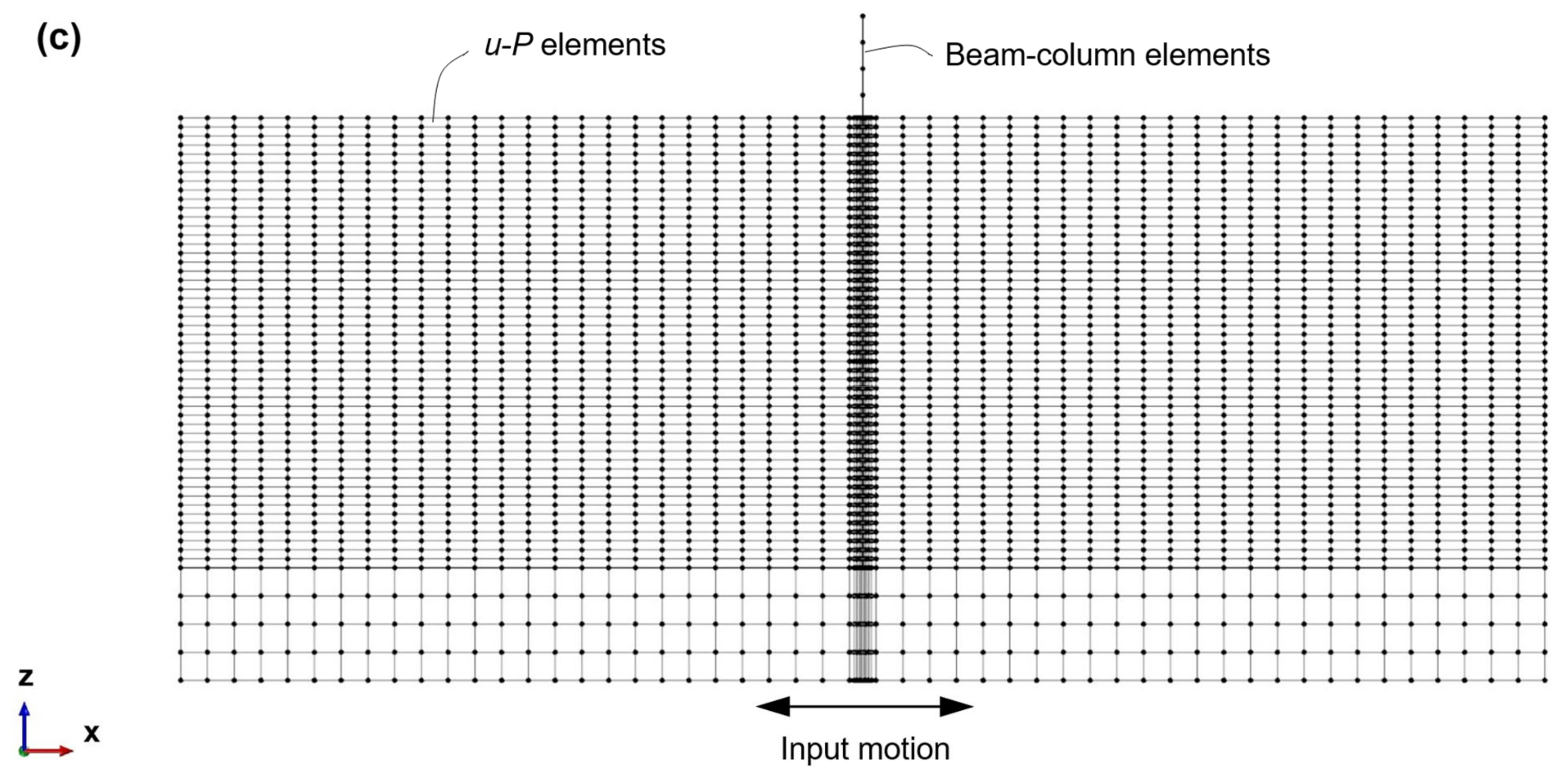
The beam–column element is used to represent the pile. This element has six DoF for each node: three for displacements and three for rotations. The structure is represented by a lumped mass on the pile head. The model’s dimensions in the x-y-z direction are 51 m × 20 m × 21 m. These dimensions were employed to avoid the effect of the FEM boundaries. The lateral boundary of the model should be sufficiently far from the model’s lower limit to minimize the impact of boundaries on the numerical results. The displacement and stress contours in the finite element software confirm that the accepted distance is enough [40,41]. The finite element meshes are built much finer (cross-shaped) near the pile, as seen in Figure 1. Also, since the seismic excitation travels vertically, the meshes are finer in the lateral direction throughout the pile depth. In order to achieve an accurate simulation of seismic wave propagation, it is necessary to ensure that the size of the mesh is less than one-tenth of the wavelength of the input frequency that has the maximum energy [7]. The mesh size was established by considering the wavelength of input motion and the highest frequency at which there was negligible spectral content. In addition, the meshing refinement should be stopped after checking that the results do not change [41]. Therefore, mesh refinement was conducted until it was confirmed that the results remained consistent.

Creating interactions between the beam–column and surrounding brick elements is a significantly challenging and critical procedure. Herein, the connection is constructed using “ASDEmbeddedNodeElement” elements. The connection detail for each pile node and adjacent nodes of soil elements is illustrated in Figure 2. Using this element, it is allowed to mesh and create the interaction without needing to provide equal depth for nodes of both surrounding soil and embedded pile elements. Soil nodes are constrained to ASDEmbeddedNodeElement for three translational DoFs as the three rotational DoFs remain unconnected.

ASDEmbeddedNodeElement can be used to embed a node inside an element in such a way that the node can move together with the element. This element was recently developed by Dr. Petracca at ASDEA software Technology, Italy [42], and serves as a constraint between constrained and multiple-retained nodes. Because in OpenSees, a Multi-Point constraint can include one retained node, this constraint was created as an Element, thereby enforcing the constraint via the Penalty method. It restricts the displacements of the constrained node to be the weighted average of the displacements of the retained nodes in its vicinity. If the constrained node has rotational DoFs, the same is done with the infinitesimal rotation.

The aim is to use a constraint attached to the joint geometries, not like an equal DoF or a rigid link, because they have some limitations; a rigid link would make the entire element act like a rigid body. Instead, with the help of this element, if a node falls inside an element, that node will move as the average motion of the element. Constraints such as equal DoFs or rigid links typically have one retained node and many constraint nodes. However, ASDEmbeddedNodeElement supports having one constraint node and multiple retained nodes. In other words, the displacement of a constraint node is the weighted average (simple interpolation) of the displacement of many retained nodes. First, one needs to create an embedded interaction to create this link. It is very important to choose “node to element” links. In this case, the retained geometry becomes a solid body, while the constraint node comes from the edge (beam).

This implicit–explicit (IMPL-EX) element (i.e., ZeroLengthContactASDimplex) is used to create a ZeroLength contact between soil–pile faces and soil–pile bottom nodes in the current work. It follows the Mohr–Coulomb criterion using a penalty-based frictional contact element. This element can utilize either a conventional Backward–Euler or IMPL-EX integration algorithm. The IMPL-EX integration executes a linear extrapolation of the internal parameters throughout the global Newton iterations. Thus, the element is linearly dependent on the trial strain. Instead, a standard implicit calculation is conducted during the committing step to partly rectify the error caused by the explicit computation. A more detailed explanation can be found in Oliver et al. [43]. The code of this element is developed for OpenSees (Version 3.6.0) at IUSS/ASDEA Software Technology, Italy [44]. This element can be used in 2D and 3D problems, allowing for 2 and 3 DoFs; and 3, 4, and 6 DoFs, respectively. Due to the fact that the two nodes can have various DoFs, the element can connect disparate components (such as solids with 3 DoFs or u–P Solids with 4 DoFs to beams/shells). Utilizing a user-defined contact vector, it is possible to be arbitrarily oriented in space. If not stated, the contact vector is assumed to be the global X-axis.

Two stiffness parameters, Kn, normal penalty stiffness for global compenetration, and Kt, tangential stiffness for frictional contact, were calculated as detailed by [43]. One of the most important features of this element is to be able to employ the IMPL-EX integration scheme, which allows the model to converge much faster, but the time steps should be smaller. Another advantage of this element is that the user can define the orientation type. For the present study, the “from link direction” orientation type is used for soil and pile interaction. With this option, one can have a physical distance between the center of the pile (beam) and the edge of the hole. When the interaction is a “Node-to-Node” link, and the distance between the two nodes is not zero, this element allows the user to choose the link direction as the contact direction. Since the original contact element in OpenSees can only be oriented in a global coordinate system, it creates various issues in modeling and solving complex problems. In addition, a rigid gap can be created when one uses “from link direction” to simulate the original “beamcontact3D” element for soil–pile interaction [45]. When using this option, the retained node must have rotational DoFs, meaning the pile (beam) should be retained, and the surrounding soil (solid) should be constrained. The convenient feature of this element is that the two nodes that need to be connected may have different DoFs. For example, one can connect a 6 DoF-node (i.e., beam) with a 3 DoF-node (i.e., standard brick element) or with a 4 DoF-node (i.e., u–P element). Therefore, since it supports any kind of DoF set, it can be used for any type of element (solid to solid, solid to beam, solid to shell, shell to beam, and so on).

In general, it is advised to use the Krylov–Newton algorithm for softening problems [46]. However, the beamcontact3D element created many convergence problems when using the Krylov–Newton solution algorithm. To overcome this problem, Newton with Line Search Algorithm could be used, but it still takes too long to reach a solution. Since the new contact element is compatible with the Krylov–Newton solution algorithm, the solution can be reached with less iteration without convergence problems.

2.3. Boundary Modeling

During the modeling of a soil body, just a part of it is modeled by utilizing artificial boundaries. In static analysis, fixed conditions at these boundaries are acceptable; however, they will reflect outgoing waves in dynamic problems. Although it is not practical due to the extensive computational effort required, this issue can be averted by employing a significant part of the model in the analysis. However, adopting unique boundary conditions that can absorb outgoing waves is an alternative solution to reduce the computational time required. For the best solution, an absorbing element should have the following three components: (1) a free–field element (F), (2) Lysmer–Kuhlemeyer dashpots (D), and (3) boundary tractions (T). Figure 3 illustrates these components in a 2D problem.

While constructing an absorbing element, the first step is to create a free–field column. It is basically responsible for computing the free–field solution. To simulate a free–field element, a free-field column should be constructed with a quad element using the equal DoFs at the size of the quad element so that the quad element is forced to move as a shear column. Therefore, for instance, if one applies equal DoFs on the vertical or horizontal displacement, this element cannot rotate, so only horizontal displacement through shear deformation would be allowed. The other component is the dashpot (D). Dashpots are responsible for absorbing outgoing waves. For example, when a wave travels from the bottom to the top of the soil, it returns back after it hits the ground surface, so one needs an absorbing boundary at the bottom to absorb outgoing waves. Similarly, suppose there is a structure on the soil domain or some imperfection when the wave reflects; it can reflect in a different direction, so absorbing boundaries on the sides is also needed. Creating dashpots was possible in the previous version of OpenSees; however, STKO offers automation by creating a ZeroLength element with viscous material.

The third component lacking in OpenSees’ previous versions was the boundary tractions (T) transferred from the free–field to the soil domain. Using the old method in OpenSees, one may experience some distortion in the boundaries of the soil domain in the displacement field. This is because the third component, “T” could not be included, as there was no element in OpenSees capable of performing the same functions as this component.

The boundary traction basically computes the stresses inside the free–field. Then, it takes the shear and horizontal stresses by projecting onto the vertical side in such a way that boundary tractions are on the left side (1–4 node side) and applies them as external forces on the two nodes of the soil domain (2–3 nodes). It is important to point out that this produces a nonsymmetric matrix because force is transferred from the free–field to the soil domain, but not on the other side. So, in 2D, one creates a quad element (for 3D, it is a hexahedron element), which is attached to the soil domain (nodes 1 to 4), and this element inside computes the solution in the free–field for nodes 1 and 4. Then, it computes the dashpots in the direction (takes the stress from the free–field and applies it to the boundaries because everything is inside the same element). Assuming the free–field has a certain motion, stress developed in the free–field should be transferred to the soil domain in such a way that nodes 3–4 on the side of the soil domain can enforce displacement of the free–field solution.

In summary, the old method was not perfect; it was very complex to achieve and error prone. Because of these aforementioned disadvantages of the old method of creating SSI, ASDEA Software Technology has recently created a new element that can actually construct absorbing boundaries with all these three components and perform all the steps automatically [47]. The ASDAbsorbingBoundary element (2D and 3D) is a macro element that computes all the components previously mentioned. This element initially acts like a constraint, and as a constraint, it will develop reactions. In the second stage, when the dynamic analysis starts, there is a specific command to activate the absorbing boundary (ASDAbsorbingBoundaryActive). When this parameter is activated (meaning, moved from stage 0 to stage 1), the element saves the previous reaction and then applies it as an external force. This element has been developed based on the work provided in [48] for the 2D case and properly improved for the 3D case [47]. One may refer to [48] and the references therein for an in-depth explanation of the theory.

Boundary conditions are implemented as follows: (1) the bottom of the mesh is completely fixed in every direction; (2) nodes along the side planes, aligned with the direction of excitation, are restricted from moving in the y direction, while those perpendicular to the excitation direction have nodes at equivalent depths constrained to exhibit identical displacements in the x direction, simulating free–field ground motion; (3) all remaining internal nodes remain free to move in all directions; and (4) pore water pressures are allowed to develop for all nodes except those corresponding to the groundwater table elevation.

The numerical simulations are executed in three loading steps. During the first step of loading, in which the pile is not added to the system, self-weight, that is, the soil and pore water weight, is applied. This phase permits the initial stress state, void ratio, and soil fabric to be developed without taking into account excavation and pile installment. These serve as initial parameters for the second step, which involves the placement of the pile and the application of its own weight as well as the weight of the structure. Then, as a final step, a dynamic nonlinear time history analysis is performed on the soil–pile–structure interaction. This stage analysis is also recommended by many researchers to avoid convergence problems [49,50].

3. Numerical Model Validation

Verification is intended to detect and eliminate errors in computer code and confirm numerical algorithms [28]. In the current work, since a complex and advanced approach is needed to simulate a pile in a 3D soil body with a coupled scheme, comprehensive verification is performed before constructing the actual model for validation. First, a simpler model with closed-form elastic solutions was verified for benchmark problems. In this regard, a single pile was created in soil layers that are not liquefiable, and performed for static vertical and horizontal loadings based on the existing literature [51,52,53]. Examination of the results revealed that the computational model could estimate with an error of about 2.5% compared to the prior studies.

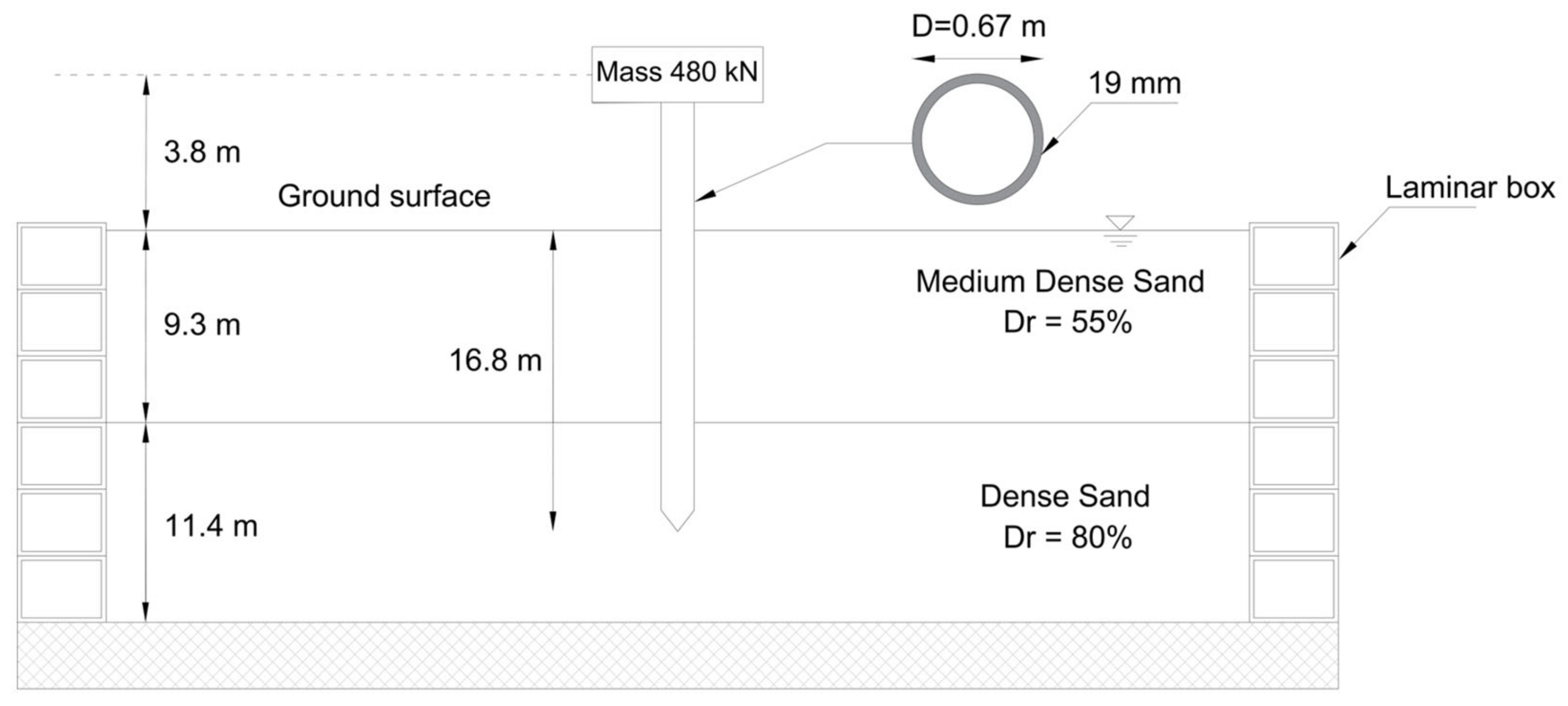
For validation purposes, centrifuge test results on SPSI at liquefiable soil sites are utilized to prove the model’s reliability for analyzing pile foundations under a seismic excitation. The dynamic centrifuge test was originally conducted by Wilson [33]. The soil profile has two horizontal layers. It is saturated, fine, and uniformly graded Nevada sand (D₅₀ = 0.15 mm, C_u = 1.5). The bottom layer (D_r = 80%) has a thickness of 11.4 m, and the top layer (D_r = 55%) has a thickness of 9.1 m based on the prototype’s scale, as shown in Figure 4. In addition, the pile corresponds to a prototype-sized steel pipe pile with a diameter of 0.67 m and a wall thickness of 19 mm. The pile head is 3.80 m above ground level and bears a superstructure load, which is 480 kN. The pile’s buried length is approximately 16.8 m.

The container was filled with a mixture of water and hydroxyl-propyl methyl-cellulose. This mixture has a viscosity around ten times that of purified water. The overall system was excited at a centrifugal acceleration of 30 g and reported that the pile remained elastic under seismic loads. As depicted in Figure 1, the FE mesh is comprised of 67,122 cubic eight-node soil elements (i.e., Brick u–P element) and 21 beam–column elements. Four elements are employed to simulate the independent pile length over the ground level, while the remaining are embedded in the soil body. Additionally, the pile head can move in each direction. Based on centrifuge modeling laws, the permeability coefficient (k) should be three times larger than the value at the prototype scale. This can be seen in

Table 2. Nevada sand material parameters (Adapted with permission from Ref. [54]).

Parameters	Units	Values for Relative Density
		Dr = 55%	Dr = 80%
Porosity (n)		0.409	0.377
Saturated unit weight (γsat)	kN/m3	19.87	20.41
Permeability coefficient (k)	m/s	6.05 × 10−5	3.7 × 10−5
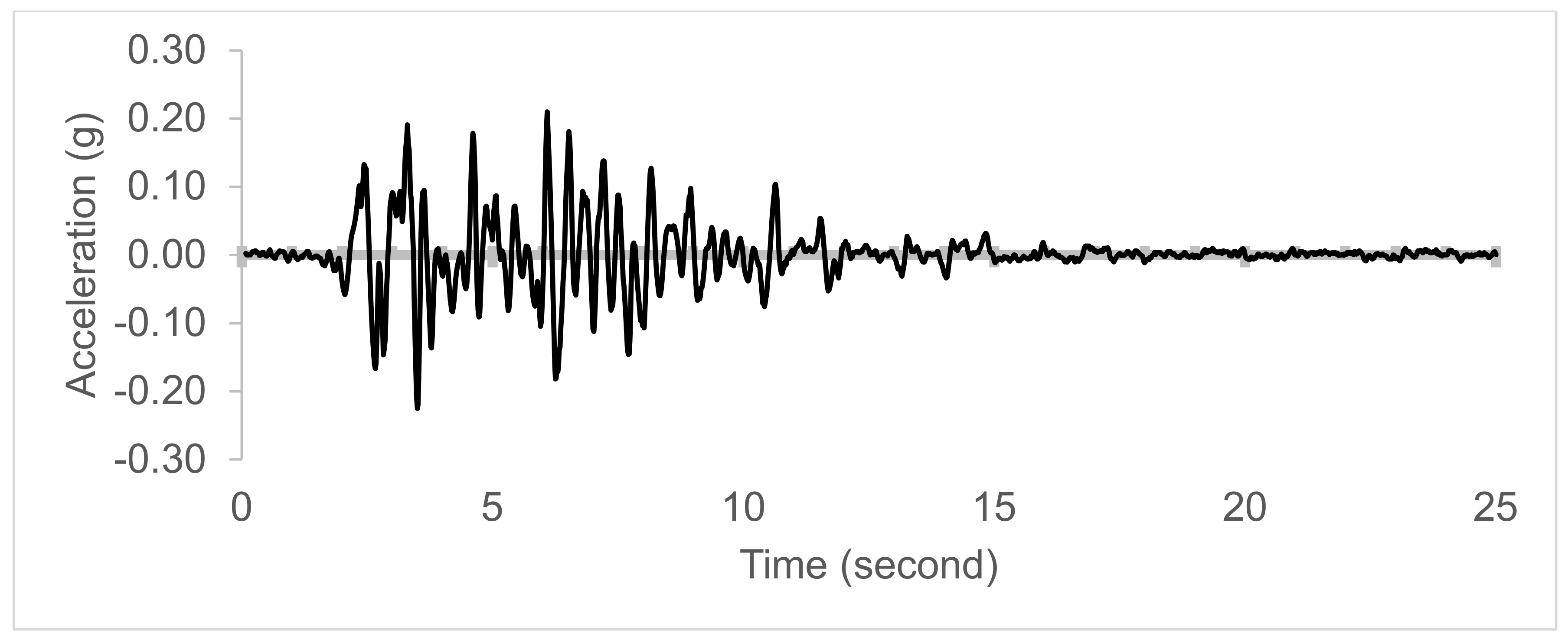
Permeability coefficient (prototype scale)	m/s	1.815 × 10−4	1.11 × 10−4

, which also presents the properties of Nevada sand adopted in the numerical model. The Kobe 1995 earthquake record is scaled to 0.22 g and used as a base input motion for the model, as shown in Figure 5.

Results

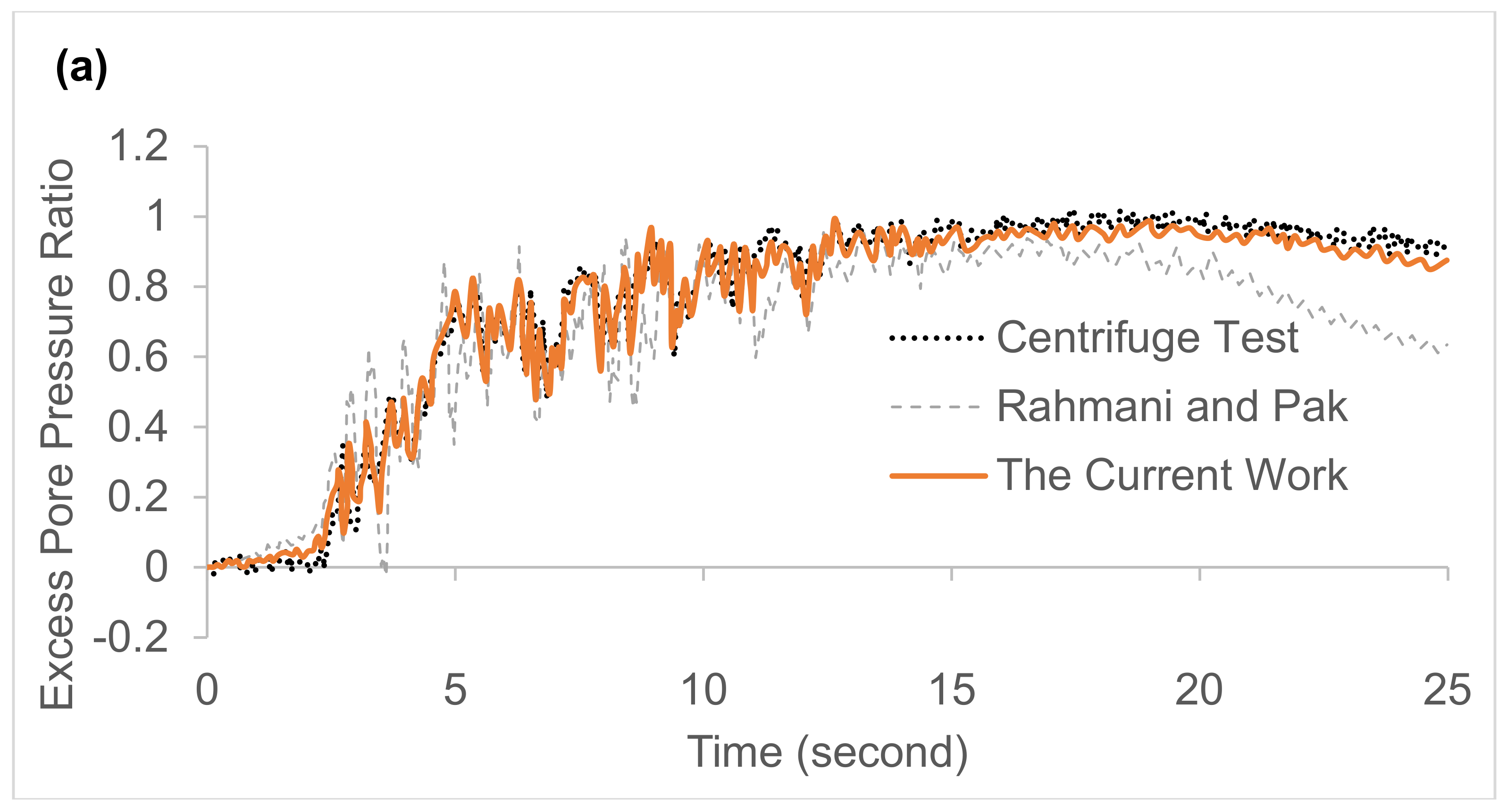
This section briefly represents the analysis results in graphs, comparing the current work results with the experimental results of Wilson [33] and the numeric results of Rahmani and Pak [20]. Figure 6 compares time histories for the recorded excess pore pressure ratios (r_u) of a centrifuge test conducted by Wilson, alongside estimated results of different 3D continuum models developed in this work and by Rahmani and Pak. The comparisons are made at depths of 1, 4.5, and 21 m in the free–field. The results show that the recorded and calculated pore water pressure levels are typically in accord.

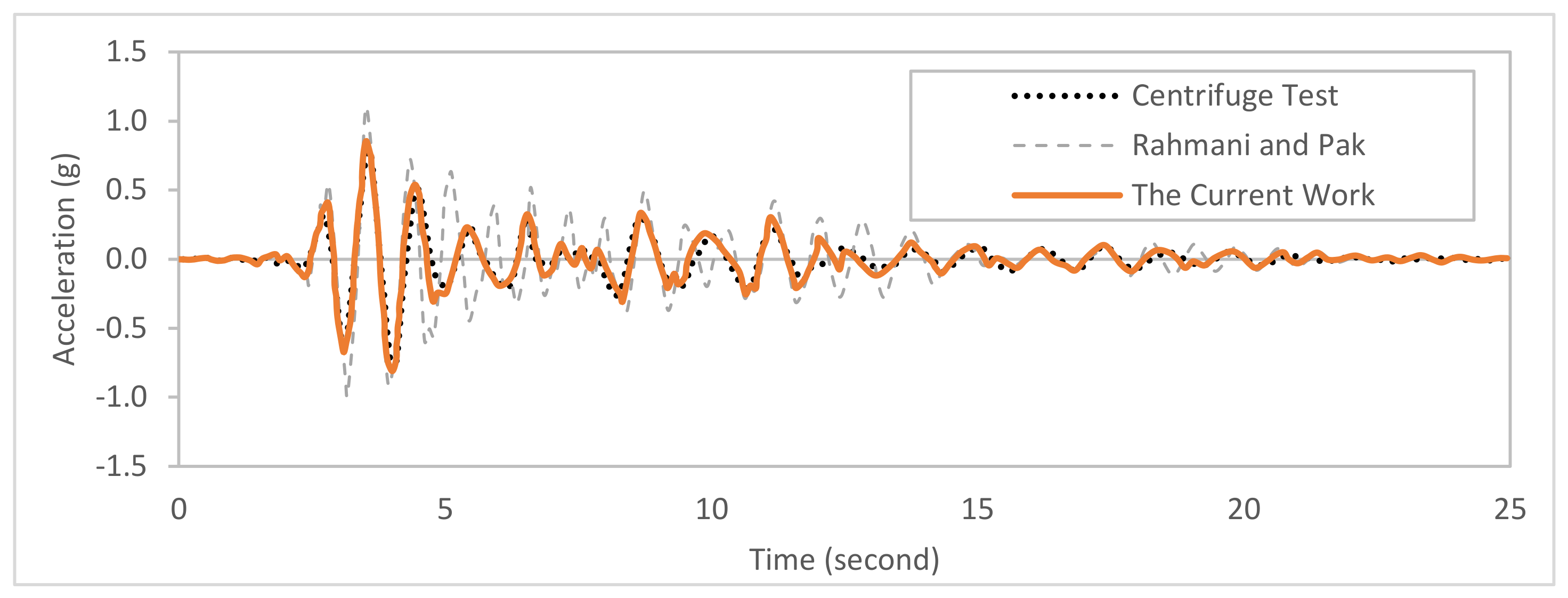
Figure 7 displays the recorded and estimated acceleration time histories of the superstructure. It also shows that the predictions of numerical simulations are comparable to the recorded acceleration values.

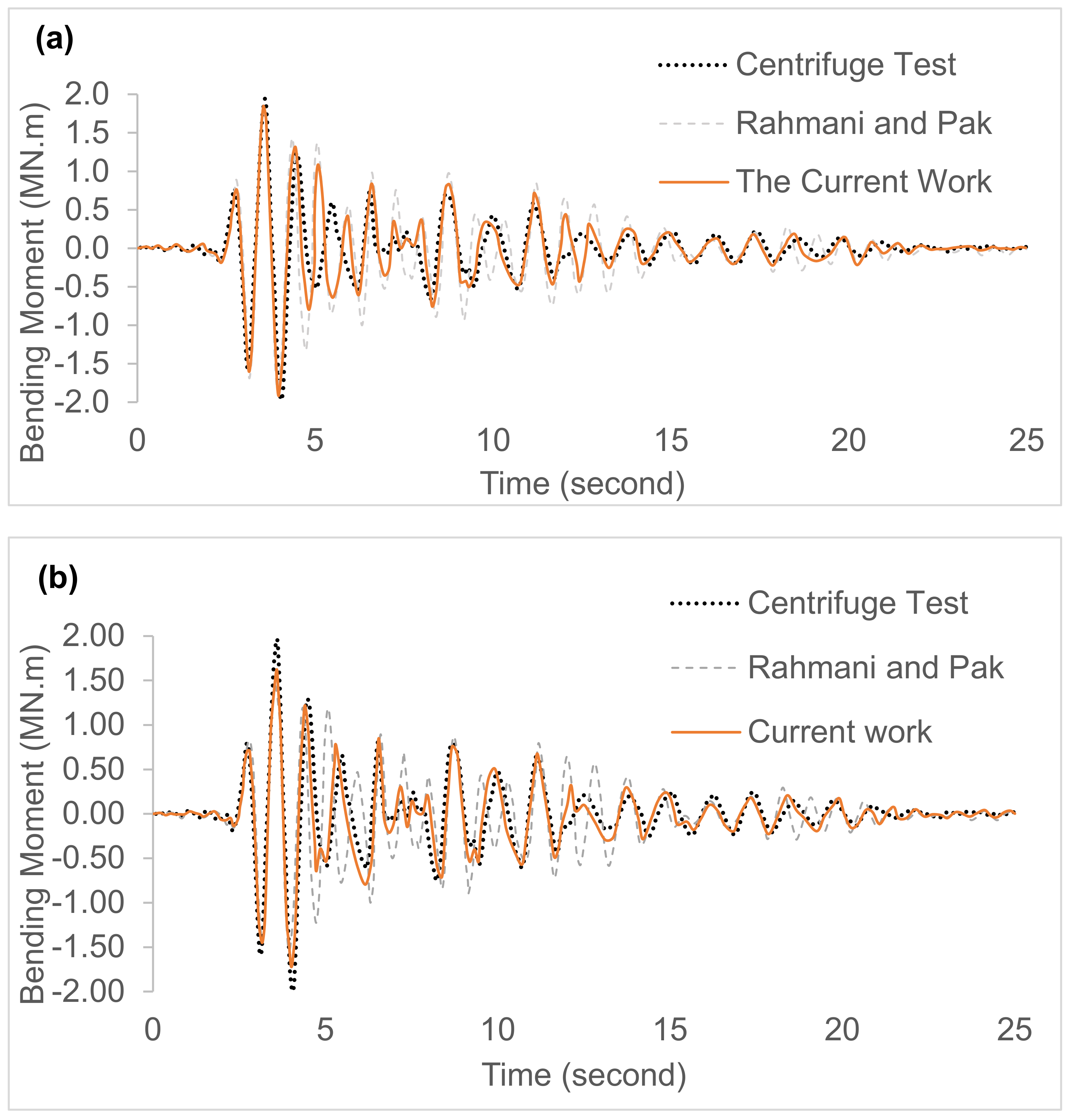
Figure 8 shows the time histories of the recorded and calculated bending moments at depths of 1 and 2 m. The results acquired from the computational models correspond closely with the values measured during the centrifuge experiment.

Lastly, Figure 9 demonstrates the time histories of ground surface settlement at 3 m away from the pile. Observations indicate that the calculated and recorded values of the settlements are also in good agreement.

In summary, it is critical to acknowledge that the results obtained using the original elements may lead to a significant overestimation of responses. This phenomenon is particularly pronounced in scenarios involving more complex and dynamically induced systems. Such discrepancies can have significant implications for engineering design and analysis, potentially resulting in conservative designs or inaccurate predictions of structural behavior. Therefore, the development and validation of new elements, as demonstrated in this study, are essential for improving the accuracy and reliability of numerical simulations, particularly in dynamic and complex structural systems, especially when considering SPSI.

4. Discussion and Recommendations

In general, the analysis results match well with the experimental results. Moreover, a better match is achieved with the newly introduced elements in OpenSees compared to the results in the literature. It is believed that the discrepancies in the results between the current study and the previous research conducted by Rahmani and Pak [20] can be attributed to several factors, namely:

Improved simulation of absorbing boundaries, leading to more accurate boundary conditions;

• Enhanced discretization, including the optimization of mesh size and model dimensions determined through preliminary calibration studies;
• A better representation of the actual behavior of the overall system, facilitated by the utilization of newly developed contact elements.
• Accordingly, the critical modeling issues of this study are discussed in this section. In addition, some recommendations and limitations are provided for potential future work.

IMPL-EX integration algorithm. In this study, the IMPL-EX integration scheme was used in the ZeroLengthContactASDimplex element to increase the robustness of the analysis. This scheme involves linearly extrapolating the internal variables through the global Newton iterations. Therefore, the element is dependent only linearly on the trial strain. A standard implicit calculation is carried out to partly correct the error caused by the explicit calculation. This accelerates the convergence of the analysis towards a stable solution and reduces the time of the analysis. This algorithm is advantageous, especially when dealing with complex simulations with strong nonlinearities.

Boundary conditions. As mentioned, since the T component was not available in the previous version of OpenSees, the user would experience unusual displacement at the soil domain edge. This is because free–field information (i.e., the stresses) cannot be transferred to the soil domain. Therefore, this is one of the reasons that the overall solution was not perfectly accurate but approximated for the previously performed SSI problems in the literature using OpenSees. On the other hand, the ASDAbsorbingBoundary element allows us to solve distortion problems at the boundaries. Using tcl code in the earlier version of OpenSees to mimic the T component was possible, but it required explicit implementation and the use of smaller time increments. However, using the ASDAbsorbingBoundary element, one can use larger time steps (standard time step) in implicit schemes.

Choosing a proper penalty value. ASDEmbeddedNodeElement imposes the constraint via the Penalty approach. This is a user-defined stiffness (K) and should be large enough to enforce the constraint but not too large; otherwise, the system may become ill conditioned. For instance, if one chooses “0”, that means there is no constraint. Suppose one chooses a value approaching infinity; that should be perfectly constrained in theory. However, in practice, it will make the system singular. Because a value that is too large makes all the other values look like zero. One may estimate this value based on the young modulus of the embedded domain multiplied by 10³ or 10⁴ (three or four order magnitude more than the young modulus). As mentioned before, ZeroLengthContactASDimplex is a penalty-based contact element. Thus, two penalty stiffnesses (i.e., Kn and Kt) should be specified for normal or tangential and penalty stiffness. Kt is typically chosen by multiplying the young modulus of the material with two- or three-order magnitude. However, it can change depending on the friction of the contact surfaces. If one does not desire to model frictional contact, Kt can be assumed to be zero (or the frictional coefficient mu = 0). Kn can be defined as in ASDEmbeddedNodeElement.

Simple modeling features. The original contact elements “ZeroLengthContact3D” and “beamcontact3D” can only be oriented in the global system. This is one of the disadvantages of these contact elements when having the pile inside a soil domain since the normal direction changes with the direction of the pile. This is why using the standard contact element is very problematic in modeling, especially for modeling many piles in a 3D continuum. In addition, the standard contact element takes many more iterations to converge, which means that when the model is complex, it will be very time-consuming to reach a solution.

In contrast, newly developed elements provide several convenient modeling features. The ZeroLengthContactASDimplex element is very advantageous for SPSI problems because it can be used for solid–beam (i.e., soil–pile) interactions for faster solutions without convergence problems, and it can also be used for solid–solid (i.e., soil–soil) interactions when one needs to create local mesh refinement to attain better stress distribution in the focused area of study. Furthermore, differently discretized meshes can be connected between the retained (typically the coarser-meshed) and the constrained (finer-meshed) domains. In the case of this type of mesh refinements, one cannot create a direct node-to-node contact using the original contact element since there is no node corresponding to every constrained node linked to a retained node. With the ZeroLengthContactASDimplex element, it is possible to create a node-to-element link to generate various meshed domains. In this case, the retained surface will represent the element part, and the constrained surface is the nodes that were in the finer-meshed solid.

When using the beamcontact3D element, one has to pay special attention to the discretization between the pile and soil because the soil node cannot be in the same direction as the pile element node. Otherwise, the node cannot find any contact node, and some numerical errors will arise. This issue is incredibly problematic when dealing with complex modeling problems because it is challenging to have each node of the solid mesh coincide with the pile mesh. The pile and soil mesh can be modeled to align with the new contact element, which is much more efficient. In addition, there is no restriction in orientation like the original contact elements have.

Regarding absorbing boundaries, while using the original method (i.e., building free–field columns around the model), there are many steps one needs to perform, such as applying the fixities, removing them for the second stage (i.e., dynamic analysis), replacing them with corresponding reactions, applying the free–field column, adding the dashpots, and so on. It is also important to note that manually creating boundaries is quite challenging and requires certain programming skills, especially in 3D because many boundary types (17 boundary types for each edge and corner) should be assigned to exact locations. However, this is much easier for users who implement the ASDAbsorbingBoundary element. In addition, automation on this matter is provided for STKO users (i.e., ASDAbsorbingBoundary3Dauto).

Finally, when using STKO, the user can use the “ignore nodes outside” feature within ASDEmbeddedNodeElement in case there are nodes outside of the embedded domain, which is the case of the current SPSI modeling in this study.

Potential applications. The newly developed elements can be implemented for applications in modeling other than SPSI. ASDEmbeddedNodeElement can be used to perform a pull-out test of an embedded bar inside a solid domain. It is also possible to connect two geometries that have incompatible meshes. For instance, a refinement for a specific domain, that is, its mesh that is much denser than the surrounding domain’s mesh, can be attached to a much coarser domain. As another example of application, one can simulate a prestressed beam by creating a solid domain to represent the beam and a cable element inside to represent the reinforced bar. These two elements can be connected using ASDEmbeddedNodeElement. Moreover, this element can be preferred for detailing reinforced concrete beam–column joints to connect the bars to the solid domains that are created for the beam and column separately. Similarly, it can be utilized to simulate a steel beam–column joint.

Epistemic and aleatory uncertainties. The uncertainties develop due to the oversimplification or the intricate nature of the numerical model of the actual system. Hence, it is crucial to highlight that both epistemic (numerical structural model definition) and aleatoric (material properties such as soil and geometry) uncertainties always impact all numerical models. This is why focusing specifically on these uncertainties is recommended to address very simple or very complex numerical modeling effectively.

5. Conclusions

This research validates newly developed elements in OpenSees for fully coupled seismic soil–pile–structure systems. As these elements are recent additions to the OpenSees library, they require critical validation, especially for soil–pile–structure interaction (SPSI) problems. This study underscores the novelty and importance of filling this gap in knowledge through validating these elements. Results are compared with experimental and numerical research, and significant findings and future recommendations are provided as follows.

(1)

The latest advancements in the OpenSees library validate its effectiveness in seismic SPSI models, enhancing accuracy in geotechnical research. Therefore, this study’s introduced elements hold promise for tackling complex SPSI problems.

(2)

The new contact and boundary elements offer several advantages over the original ones: (i) practical modeling in complex problems, (ii) increased accuracy in results, and (iii) being less error prone.

(3)

In Figure 6, an abrupt decrease in pore pressure corresponds to sudden acceleration peaks, indicating a temporary increase in soil stiffness. This facilitates the transmission of significant acceleration peaks from the ground to the superstructure, as noted in Rahmani and Pak [20]. The current work shows improved simulation of this transmission, with superstructure acceleration values aligning more closely with centrifuge results.

(4)

Based on estimated and recorded results, the maximum bending moment at 1 m depth develops at t = 3.5 s, coinciding with an abrupt rise in the pore pressure softening the neighboring soil. When t = 3.5 s, maximum acceleration at the pile top induces significant inertial forces at the shaft, as shown in Figure 7. Therefore, the maximum moments at this point result from both soil softening and the inertial forces formed at the pile head. Additionally, the improved match in bending moment time histories (see Figure 8) suggests more accurate soil–pile contact has been established.

(5)

Based on the time histories in Figure 9, the settlement calculated 3 m distant from the pile closely matches the experimental results. This suggests highly effective interaction within the system.

(6)

While the findings closely align with Wilson’s experimental test [33] and outperform Rahmani and Pak’s [20] numerical simulation using the original elements, discernible disparities remain. The differences may stem from variations in constitutive models, contact element stiffness, mesh size, and model dimensions. Further investigation into these disparities is warranted in future research.

In conclusion, this research focused specifically on a single-pile simulation with a simplified lumped mass representation of the superstructure. Therefore, future research should expand to include more complex superstructures and compare with experimental data to address this limitation. Potential areas for future exploration include large structures such as bridges and tall buildings, which incorporate multiple interaction elements, various materials, and configurations involving pile groups and inclined piles.