

Evaluating the Performance of a Combined Vertical Wall–Horizontal Roof Solar Chimney for the Natural Ventilation of Buildings

Abstract
1. Introduction
2. Numerical Method
2.1. Governing Equations
- Boussinesq approximation was adapted for the variation of the air properties with temperature.
- The flow and thermal characteristics of the solar chimney were determined according to the heat transfer from the inner surface to the air inside the cavity. Accordingly, the solar heat gain was modeled with a heat source distributed on one side of the air cavity.
- The governing equations were discretized with the Finite Volume Method facilitated with the commercial CFD software Ansys Fluent (Academic version).
- Radiative heat transfer among the inner surfaces of the cavity was computed with the S2S model available in Ansys Fluent.
- The SIMPLEC method for pressure–velocity coupling.
- The PRESTO! Scheme for the discretization of the pressure term.
- Second-order discretization for all equations.
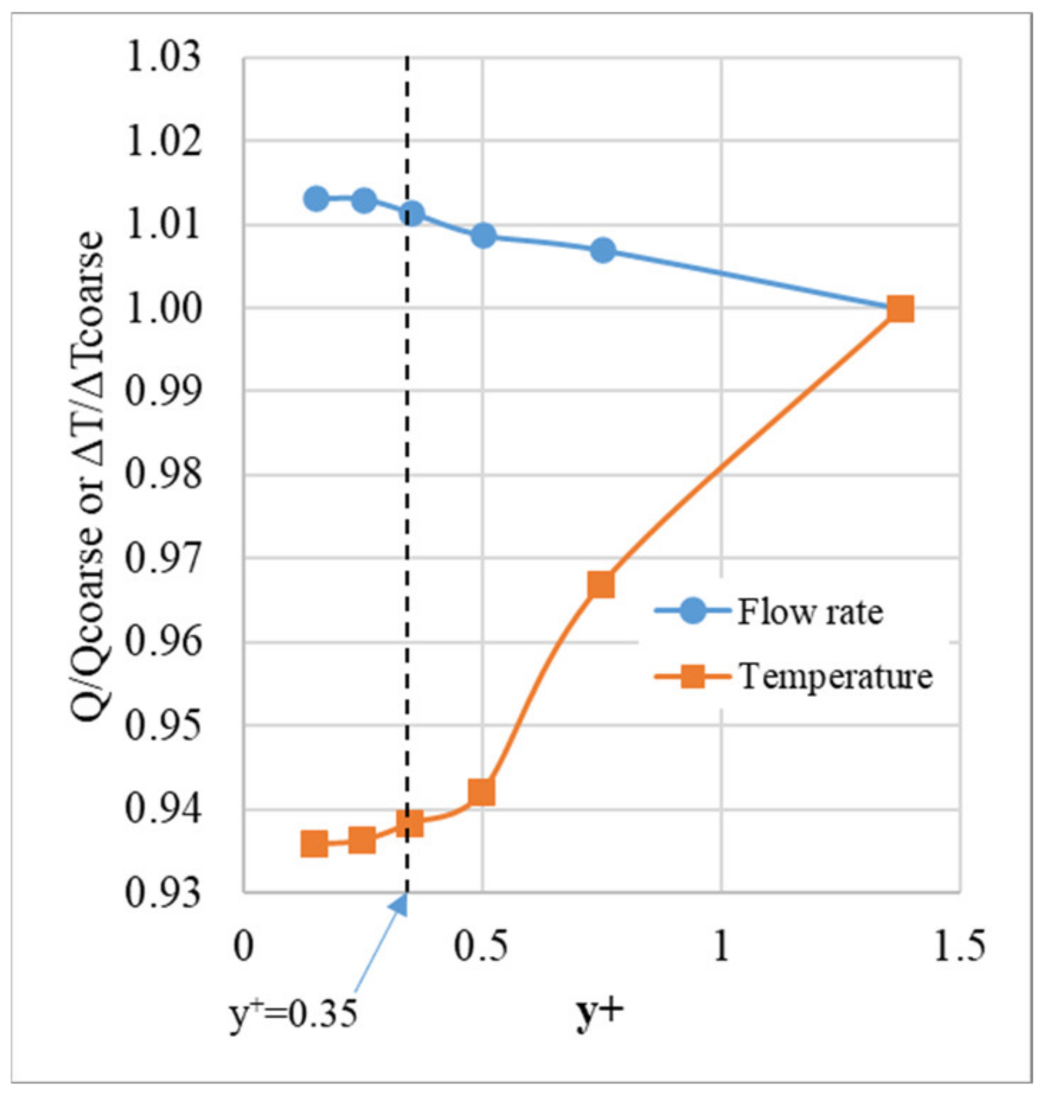
- A standard wall function for the near-wall treatment. However, as seen in Section 2.2, the employed mesh had several cells inside the laminar viscous sublayer, meaning a wall function was not required [25].
2.2. Computational Domain, Mesh, and Boundary Conditions
- Atmospheric pressure and temperature were applied on the domain boundary to allow ambient air to freely enter and leave the domain.
- All solid surfaces were non-slip surfaces.
- A uniform heat flux, I, of was applied on either side of the air cavity in two cases, namely in heating the upper and lower walls, as displayed in Figure 1a to represent two cases of the absorbing surface of the chimney. A chimney with opaque upper walls absorbs solar radiation on the upper walls. Accordingly, the upper walls are heated by solar radiation. The absorbed heat is then transferred to the air in the cavity from the inner surfaces of the upper walls. Therefore, this case is named “heating the upper walls (HUW)”. On the other hand, with transparent upper walls such as glass-plate walls, solar radiation is transmitted through the upper walls, heats the lower surfaces, and then is transferred to the air in the cavity. Consequently, this case is named “heating the lower walls (HLW)”. With the dimensions denoted in Figure 1a, the heating length of the upper and lower surfaces are and , respectively.
- Other solid walls were adiabatic.
2.3. Validation
3. Results and Discussion
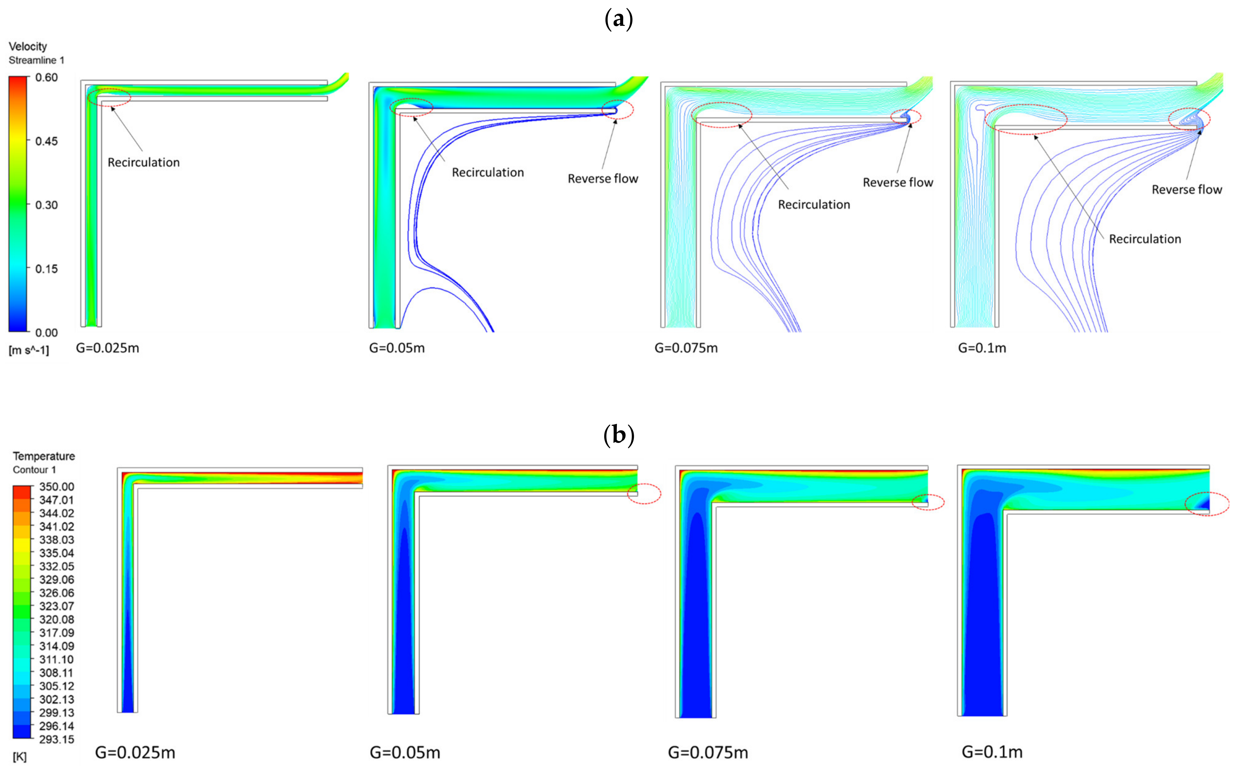
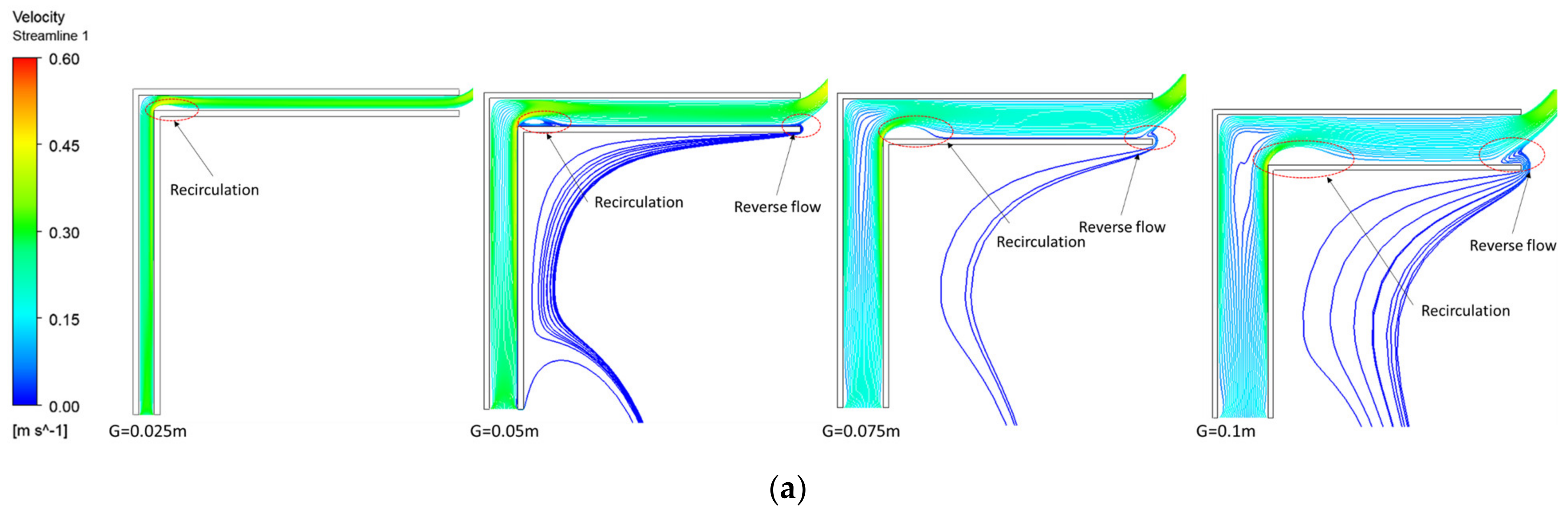
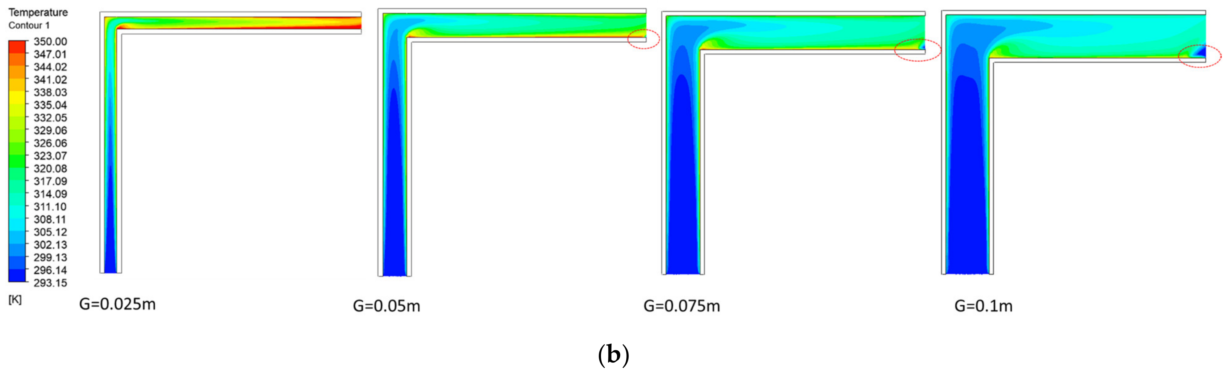
3.1. Flow and Temperature Fields
- The flow velocity and temperature decrease, particularly in the L portion.
- A recirculation occurs at all gaps, but its size enlarges as G increases.
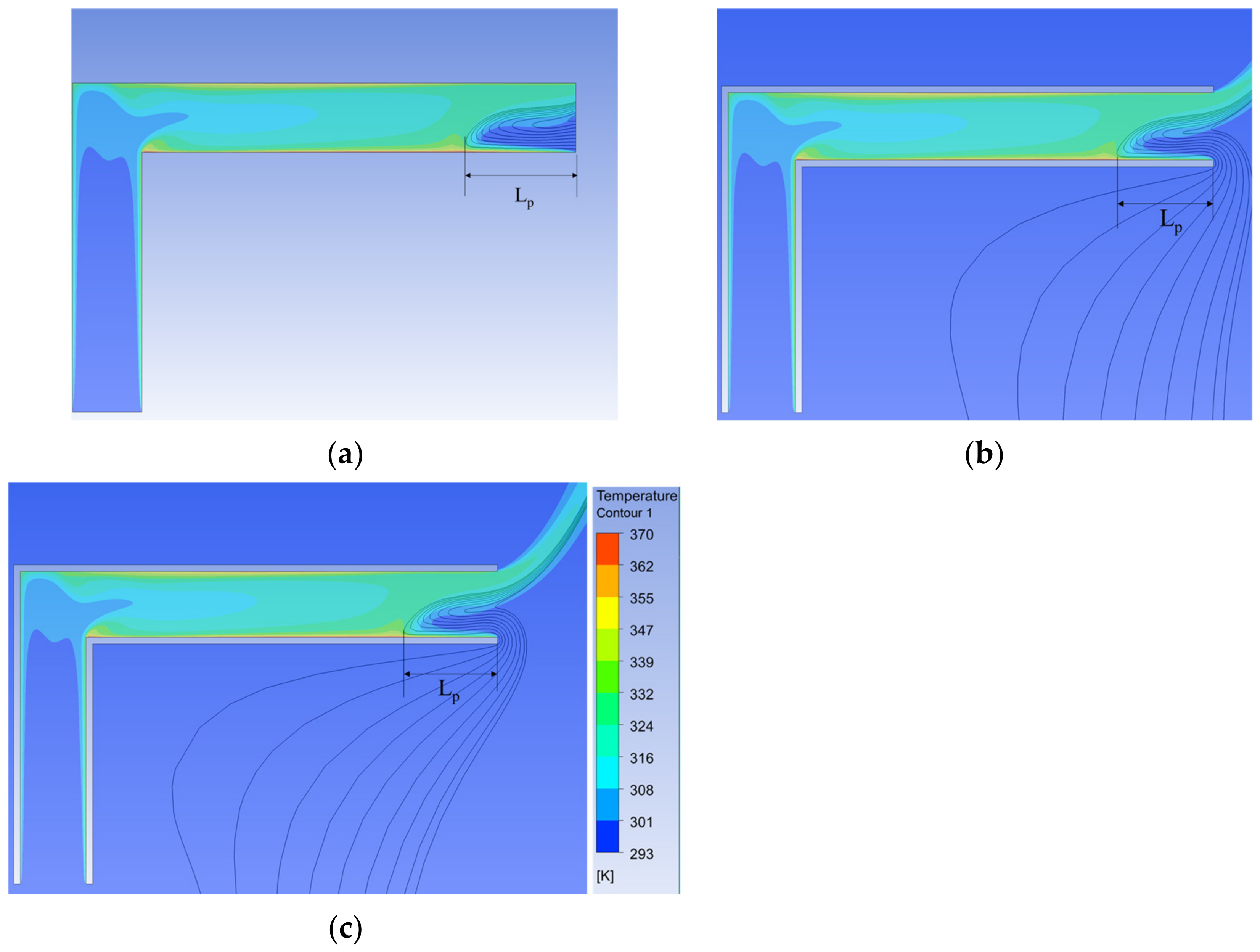
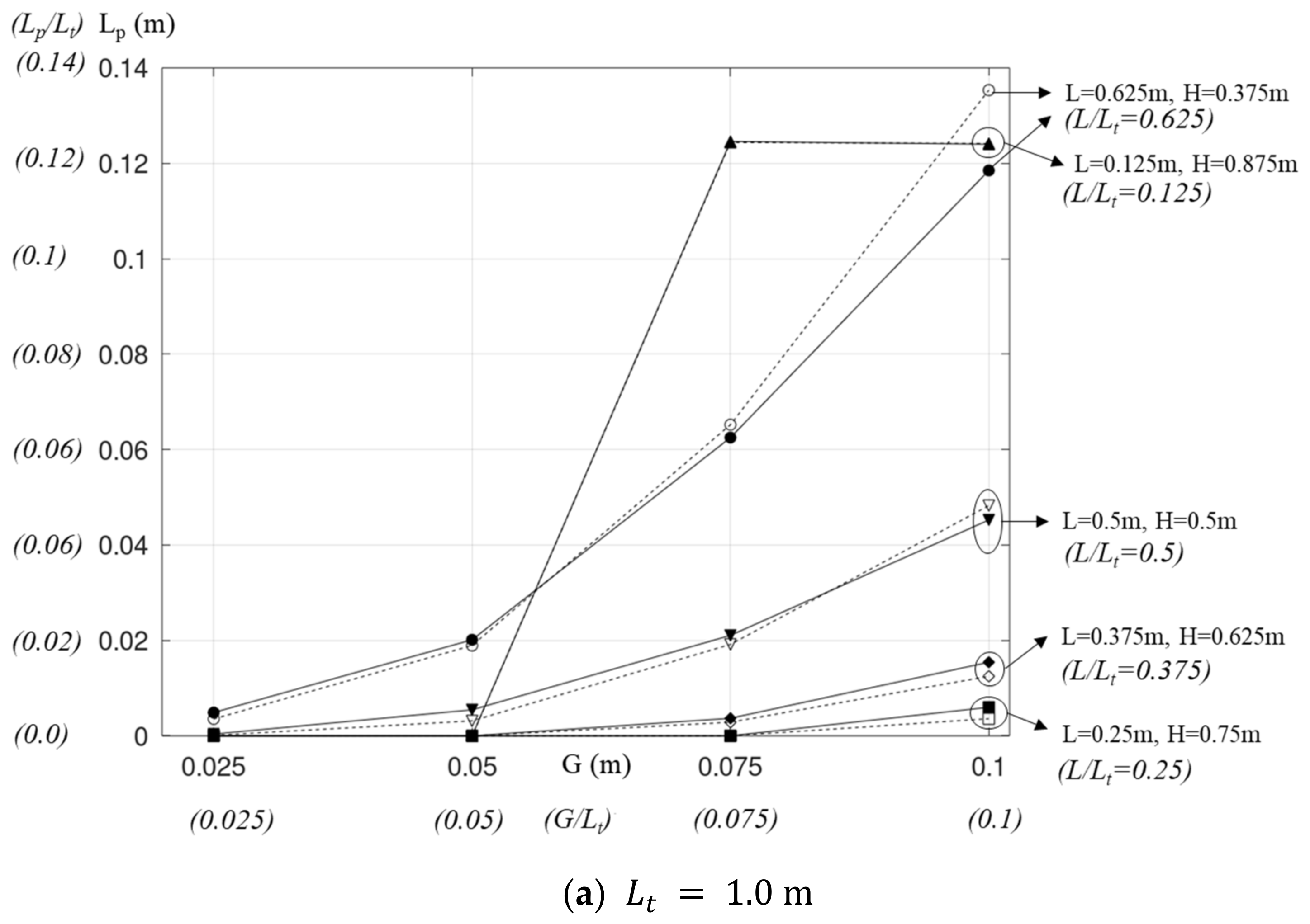
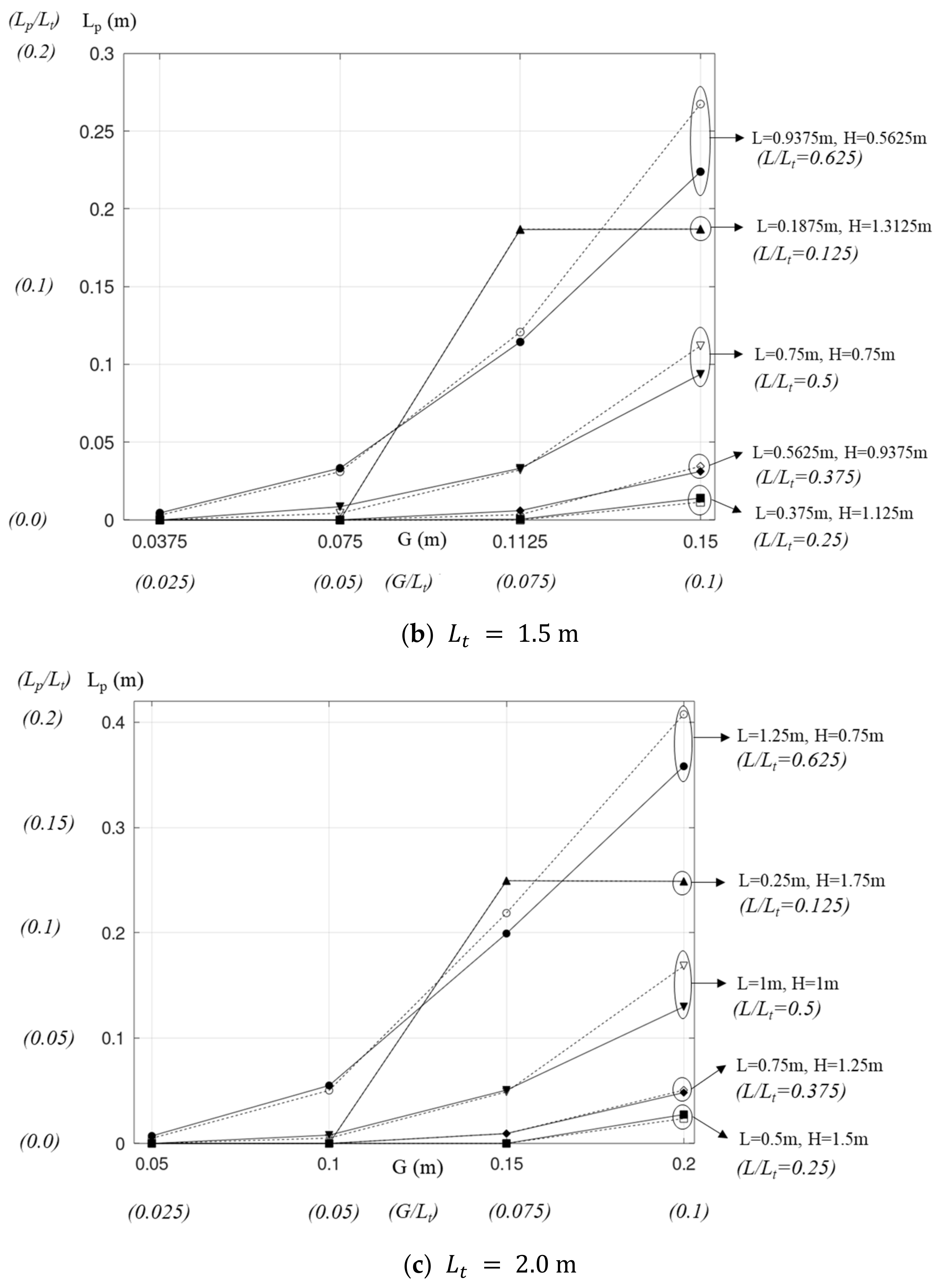
3.2. Length of the Reverse Flow
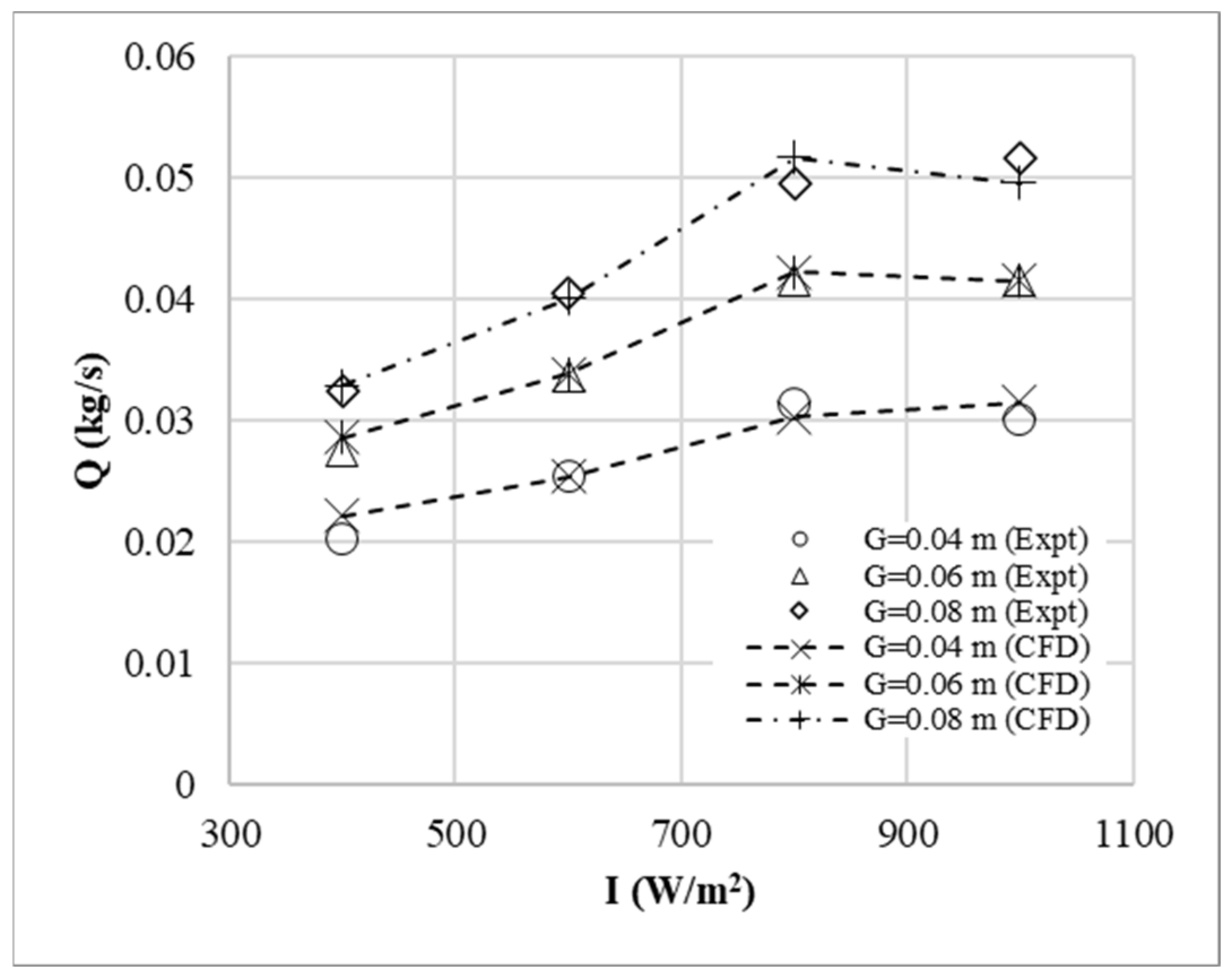
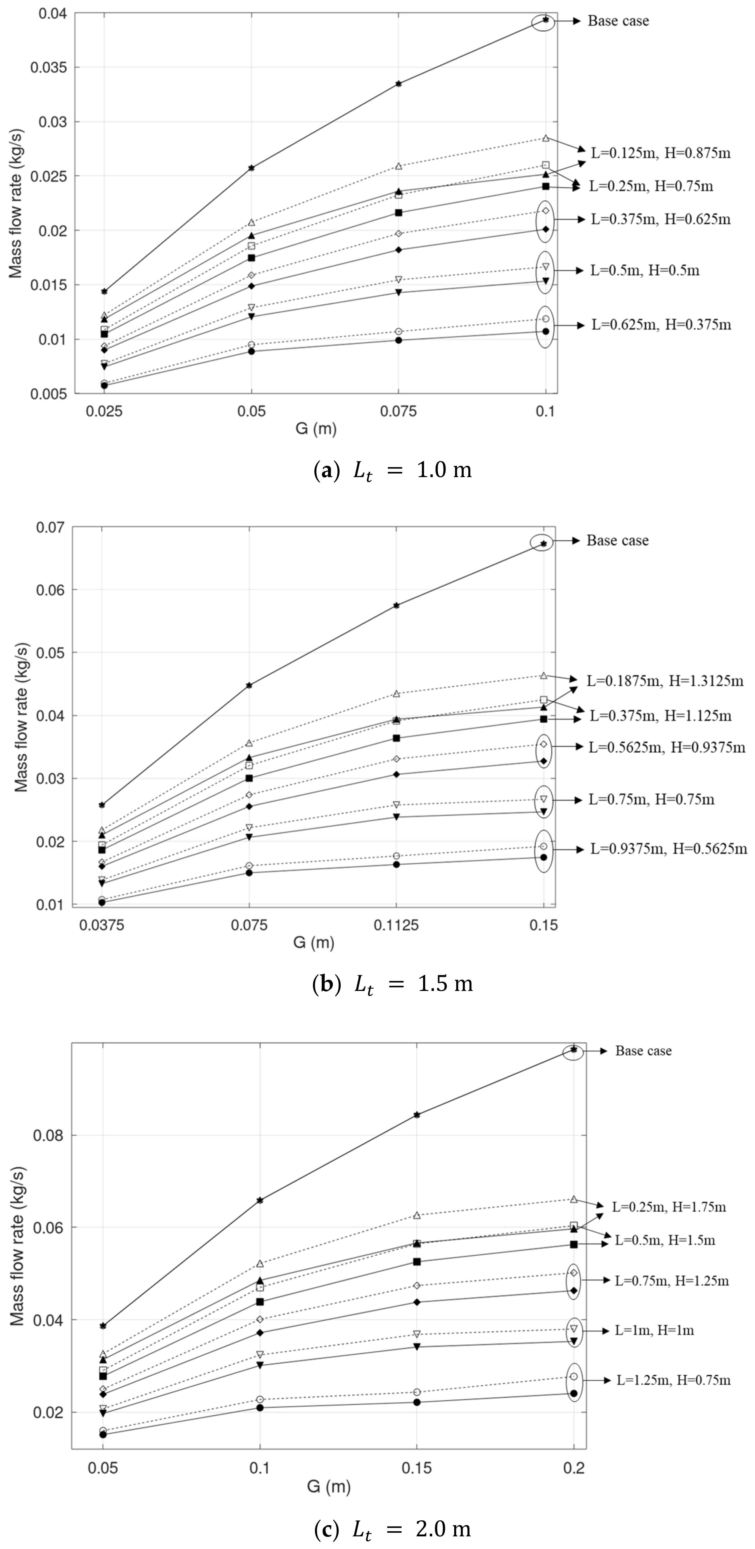
3.3. Mass Flow Rate
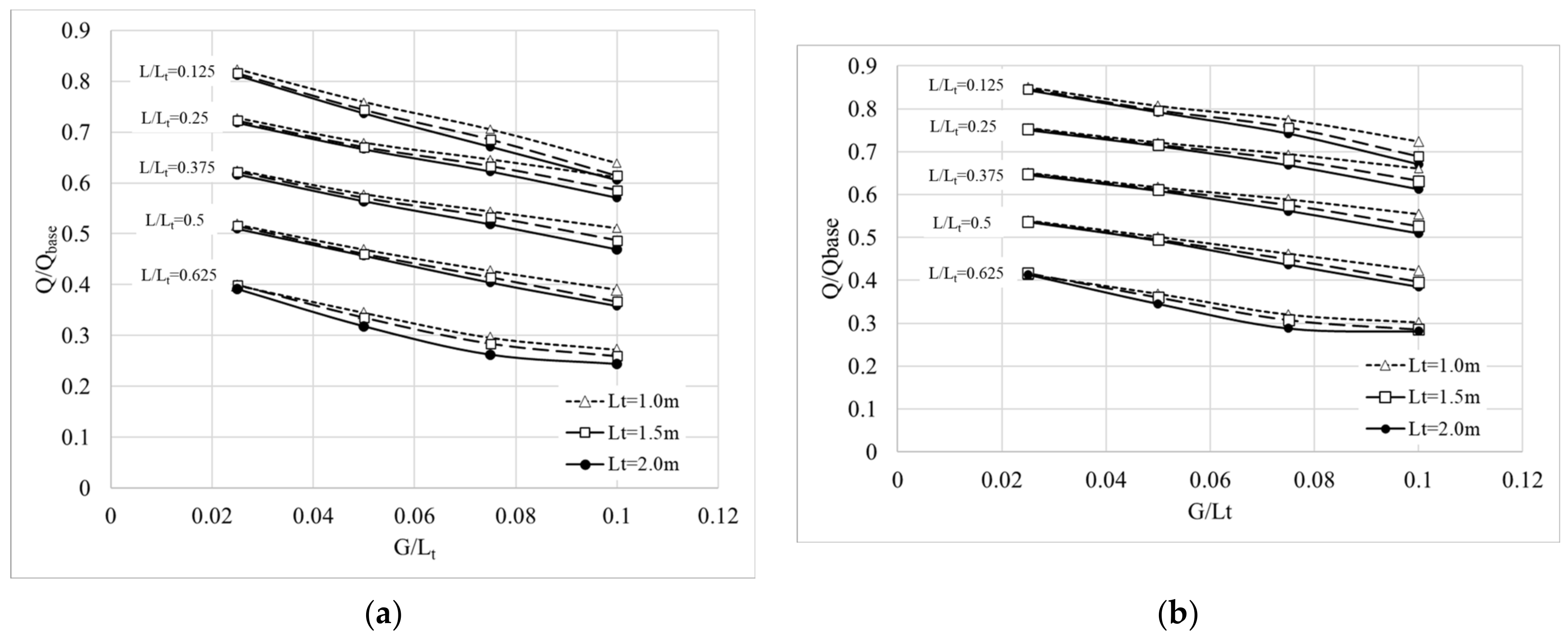
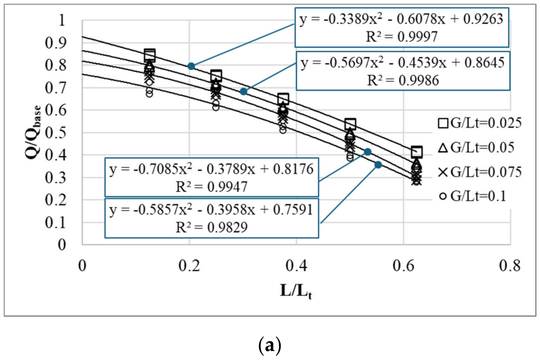
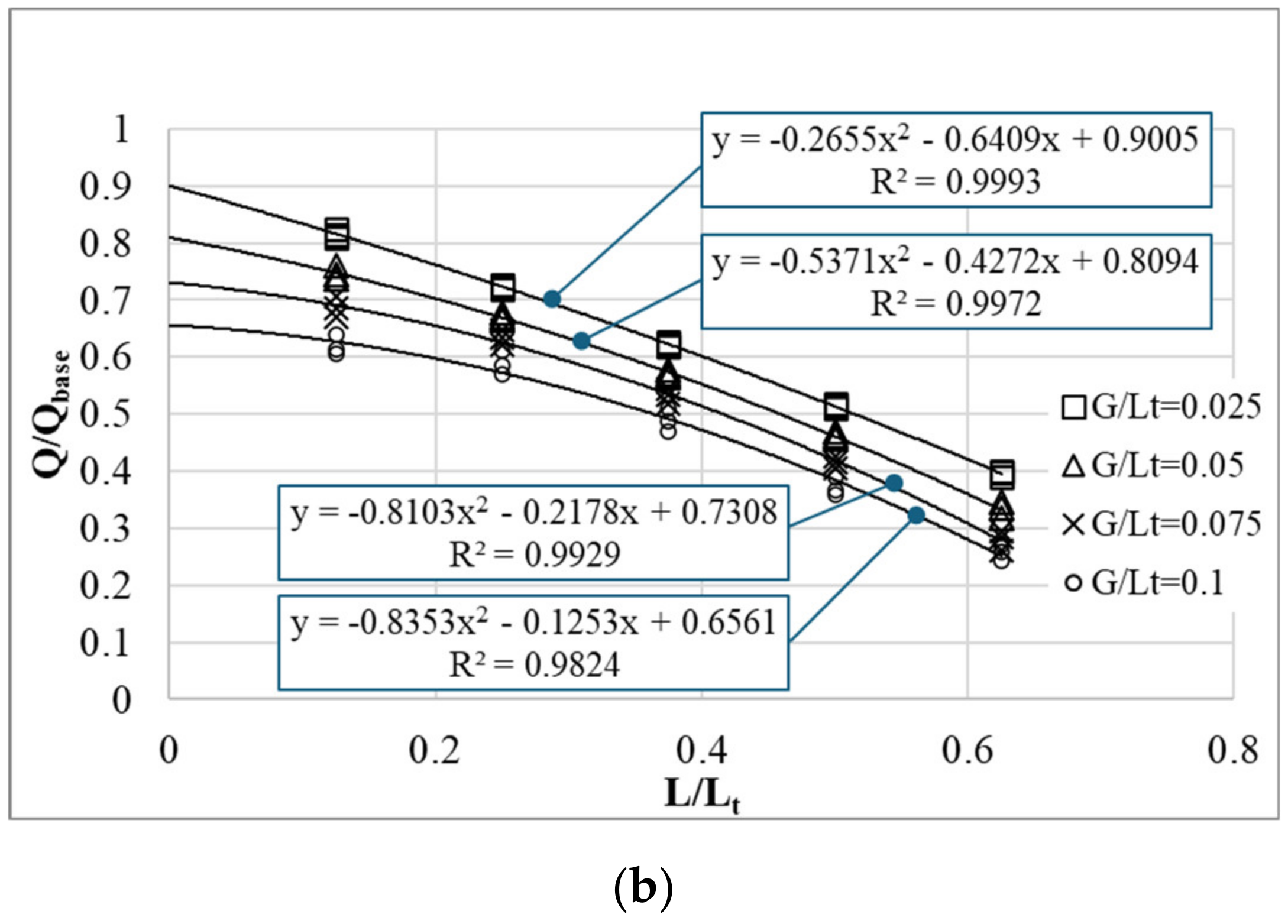
- decreases as increases, showing that the increasing rate of the flow rate versus the gap in the combined case is less than that in the base case.
- depends on but is almost independent of . The differences among the scaled flow rates of the three values of at a value of increases with , but the maximum discrepancy is only 5.0%.
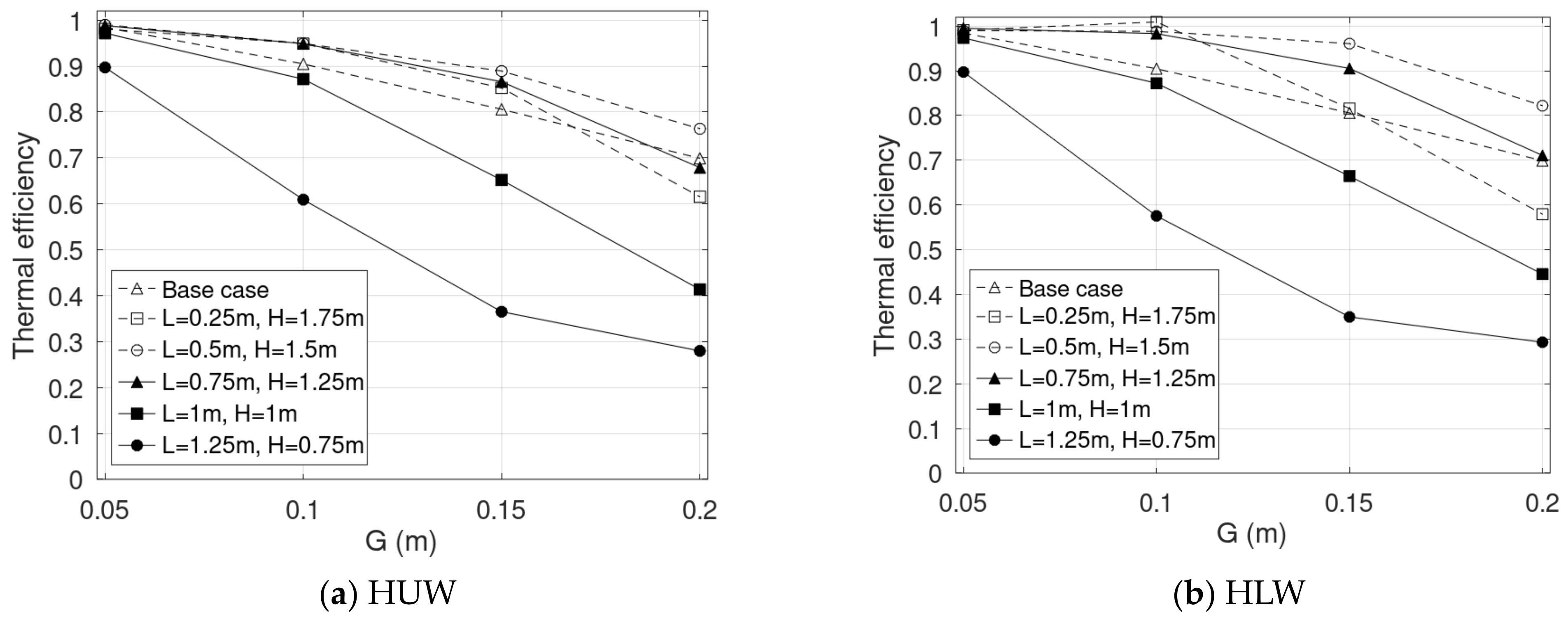
3.4. Thermal Efficiency
- decreases as the gap increases. This observation applies to both the base and the combined solar chimneys and aligns with the results reported in the literature.
- Increasing results in a decrease in . However, for , the highest is obtained with .
- of the base case is close to that of the case where .
- slightly decreases as increases, as seen for both the base and the combined chimneys.
- HLW shows a higher thermal efficiency than HUW.
4. Conclusions
Author Contributions
Funding
Data Availability Statement
Conflicts of Interest
Nomenclature
| non-dimensional maximal distance of the first cells on the walls,, where is the friction velocity (m/s) and is the distance of the first mesh cell from the wall; | |
| thermal diffusivity of air (); | |
| thermal expansion coefficient of air (1/K); | |
| thermal efficiency; | |
| thermal conductivity (W/m·K); | |
| kinematic viscosity of air (); | |
| density of air (); | |
| turbulent kinetic energy dissipation rate (); | |
| A | heating length (m); |
| CFD | Computational Fluid Dynamics; |
| Expt. | experiment; |
| G | chimney gap (m); |
| g | gravitational acceleration (); |
| H | height of the wall section (m); |
| I | heat flux (); |
| L | length of the roof section or total length or length of the reverse-flow zone (m); |
| p | pressure (Pa); |
| Pr | Prandtl number; |
| Q | mass flow rate (kg/s); |
| Ra | Rayleigh number; |
| T | time-averaged temperature (K); |
| u | velocity (m/s); |
| turbulence kinetic energy (). | |
| Subscripts: | |
| a | ambient; |
| base | base case; |
| e | extension; |
| HLW | heating the lower walls; |
| HUW | heating the upper walls; |
| p | reverse flow; |
| o | outlet; |
| sc | case of no domain extension; |
| t | total. |
| Superscripts: | |
| fluctuating component; | |
| time-averaged. | |
References
- Shi, L.; Ziem, A.; Zhang, G.; Li, J.; Setunge, S. Solar chimney for a real building considering both energy-saving and fire safety—A case study. Energy Build. 2020, 221, 110016. [Google Scholar] [CrossRef]
- Miyazaki, T.; Akisawa, A.; Kashiwagi, T. The effects of solar chimneys on thermal load mitigation of office buildings under the Japanese climate. Renew. Energy 2006, 31, 987–1010. [Google Scholar] [CrossRef]
- Al Touma, A.; Ouahrani, D. Performance assessment of evaporatively-cooled window driven by solar chimney in hot and humid climates. Sol. Energy 2018, 169, 187–195. [Google Scholar] [CrossRef]
- Zhou, Y.; Ni, M. Feasibility study on applications of solar chimney and earth tube systems for BEAM/LEED assessment: Ventilation and energy efficiency. Int. J. Energy Res. 2016, 40, 1207–1220. [Google Scholar] [CrossRef]
- Shi, L.; Zhang, G.; Yang, W.; Huang, D.; Cheng, X.; Setunge, S. Determining the influencing factors on the performance of solar chimney in buildings. Renew. Sustain. Energy Rev. 2018, 88, 223–238. [Google Scholar] [CrossRef]
- Nguyen, Y.Q.; Wells, J.C. A numerical study on induced flowrate and thermal efficiency of a solar chimney with horizontal absorber surface for ventilation of buildings. J. Build. Eng. 2020, 28, 101050. [Google Scholar] [CrossRef]
- Nguyen, Y.Q.; Wells, J.C. Effects of wall proximity on the airflow in a vertical solar chimney for natural ventilation of dwellings. J. Build. Phys. 2020, 44, 174425912090951. [Google Scholar] [CrossRef]
- Zavala-Guillén, I.; Xamán, J.; Hernández-Pérez, I.; Hernández-Lopéz, I.; Gijón-Rivera, M.; Chávez, Y. Numerical study of the optimum width of 2a diurnal double air-channel solar chimney. Energy 2018, 147, 403–417. [Google Scholar] [CrossRef]
- Zhang, T.; Yang, H. Flow and heat transfer characteristics of natural convection in vertical air channels of double-skin solar façades. Appl. Energy 2019, 242, 107–120. [Google Scholar] [CrossRef]
- Nguyen, Y.Q.; Nguyen, V.T. Characterizing the induced flow through the cavity of a wall solar chimney under the effects of the opening heights. J. Build. Phys. 2023, 46, 630–653. [Google Scholar] [CrossRef]
- Al-Kayiem, H.H.; Sreejaya, K.V.; Chikere, A.O. Experimental and numerical analysis of the influence of inlet configuration on the performance of a roof top solar chimney. Energy Build. 2018, 159, 89–98. [Google Scholar] [CrossRef]
- Chen, Z.D.; Bandopadhayay, P.; Halldorsson, J.; Byrjalsen, C.; Heiselberg, P.; Li, Y. An experimental investigation of a solar chimney model with uniform wall heat flux. Build. Environ. 2003, 38, 893–906. [Google Scholar] [CrossRef]
- Bassiouny, R.; Korah, N.S.A. Effect of solar chimney inclination angle on space flow pattern and ventilation rate. Energy Build. 2009, 41, 190–196. [Google Scholar] [CrossRef]
- Harris, D.J.; Helwig, N. Solar chimney and building ventilation. Appl. Energy 2007, 84, 135–146. [Google Scholar] [CrossRef]
- Wang, Q.; Zhang, G.; Wu, Q.; Li, W.; Shi, L. A combined wall and roof solar chimney in one building. Energy 2022, 240, 122480. [Google Scholar] [CrossRef]
- Liu, H.; Li, P.; Yu, B.; Zhang, M.; Tan, Q.; Wang, Y.; Zhang, Y. Contrastive Analysis on the Ventilation Performance of a Combined Solar Chimney. Appl. Sci. 2021, 12, 156. [Google Scholar] [CrossRef]
- AboulNaga, M.M.; Abdrabboh, S.N. Improving night ventilation into low-rise buildings in hot-arid climates exploring a combined wall–roof solar chimney. Renew. Energy 2000, 19, 47–54. [Google Scholar] [CrossRef]
- Wei, D. A study of the ventilation performance of a series of connected solar chimneys integrated with building. Renew. Energy 2011, 36, 265–271. [Google Scholar] [CrossRef]
- Serageldin, A.A.; Abdelrahman, A.K.; Ookawara, S. Parametric study and optimization of a solar chimney passive ventilation system coupled with an earth-to-air heat exchanger. Sustain. Energy Technol. Assess. 2018, 30, 263–278. [Google Scholar] [CrossRef]
- Nguyen, Y.Q.; Nguyen, V.T.; Tran, L.T.; Wells, J.C. CFD Analysis of Different Ventilation Strategies for a Room with a Heated Wall. Buildings 2022, 12, 1300. [Google Scholar] [CrossRef]
- Jing, H.; Chen, Z.; Li, A. Experimental study of the prediction of the ventilation flow rate through solar chimney with large gap-to-height ratios. Build. Environ. 2015, 89, 150–159. [Google Scholar] [CrossRef]
- Khanal, R.; Lei, C. Flow reversal effects on buoyancy induced air flow in a solar chimney. Sol. Energy 2012, 86, 9. [Google Scholar] [CrossRef]
- Ren, X.-H.; Liu, R.-Z.; Wang, Y.-H.; Wang, L.; Zhao, F.-Y. Thermal driven natural convective flows inside the solar chimney flush-mounted with discrete heating sources: Reversal and cooperative flow dynamics. Renew. Energy 2019, 138, 354–367. [Google Scholar] [CrossRef]
- Kim, K.M.; Nguyen, D.H.; Shim, G.H.; Jerng, D.-W.; Ahn, H.S. Experimental study of turbulent air natural convection in open-ended vertical parallel plates under asymmetric heating conditions. Int. J. Heat Mass Transf. 2020, 159, 120135. [Google Scholar] [CrossRef]
- Zamora, B.; Kaiser, A.S. Optimum wall-to-wall spacing in solar chimney shaped channels in natural convection by numerical investigation. Appl. Therm. Eng. 2009, 29, 762–769. [Google Scholar] [CrossRef]
- Gan, G. Impact of computational domain on the prediction of buoyancy-driven ventilation cooling. Build. Environ. 2010, 45, 1173–1183. [Google Scholar] [CrossRef]
- Burek, S.A.M.; Habeb, A. Air flow and thermal efficiency characteristics in solar chimneys and Trombe Walls. Energy Build. 2007, 39, 128–135. [Google Scholar] [CrossRef]
- Bouchair, A. Solar chimney for promoting cooling ventilation in southern Algeria. Build. Serv. Eng. Res. Technol. 1994, 15, 81–93. [Google Scholar] [CrossRef]
- Nguyen, Y.Q. Studying convective flow in a vertical solar chimney at low Rayleigh number by Lattice Boltzmann Method: A simple method to suppress the reverse flow at outlet. In Proceedings of the International Conference on Advances in Computational Mechanics 2017, ACOME 2017, Phu Quoc Island, Vietnam, 2–4 August 2017; Nguyen-Xuan, H., Phung-Van, P., Rabczuk, T., Eds.; Lecture Notes in Mechanical Engineering. Springer: Singapore, 2018. [Google Scholar]
- Nguyen, Y.Q.; Nguyen-Tan, S.T.; Pham, H.-T.; Manh-Thuy, A.; Huynh-Nhat, T. Performance of a Solar Chimney for Cooling Building Façades under Different Heat Source Distributions in the Air Channel. Int. J. Adv. Sci. Eng. Inf. Technol. 2021, 11, 158–164. [Google Scholar] [CrossRef]
- Ong, K.S. A mathematical model of a solar chimney. Renew. Energy 2003, 28, 1047–1060. [Google Scholar] [CrossRef]


| Case G = 0.05 m H = 0.5 m, L = 0.5 m | Case G = 0.1 m H = 0.375 m, L = 0.625 m | |||
|---|---|---|---|---|
| Q/Qsc | ΔT/ΔTsc | Q/Qsc | ΔT/ΔTsc | |
| 0 | 1.000 | 1.000 | 1.000 | 1.000 |
| 5 G | 0.992 | 1.014 | 1.004 | 1.017 |
| 10 G | 0.993 | 1.013 | 1.007 | 1.017 |
| (m) | Rayleigh Number | Base Case | Combined Solar Chimney | ||||
|---|---|---|---|---|---|---|---|
| L (m) | H (m) | L (m) | H (m) | G (m) | |||
| 1.0 | 0 | 1.0 | 0.125–0.625 | 0.875–0.375 | 0.025–0.1 | 0.025–0.1 | |
| 1.5 | 0 | 1.5 | 0.1875–0.9735 | 1.3125–0.5625 | 0.375–0.15 | ||
| 2.0 | 0 | 2.0 | 0.25–1.5 | 1.75–0.5 | 0.05–0.2 | ||
| 0.125 | 0.05 | 0.05 | 0.05 |
| 0.25 | 0.075 | 0.075 | 0.075 |
| 0.375 | 0.05 | 0.05 | 0.05 |
| 0.5 | 0.025 | 0.025 | 0.025 |
| 0.625 | <0.025 | <0.025 | <0.025 |
| 0.125 | 0.025 | 1.05 | 1.03 | 1.04 | 1.04 |
| 0.05 | 1.10 | 1.06 | 1.07 | 1.08 | |
| 0.075 | 1.15 | 1.10 | 1.10 | 1.11 | |
| 0.1 | 1.2 | 1.13 | 1.12 | 1.11 | |
| 0.25 | 0.025 | 1.05 | 1.04 | 1.04 | 1.05 |
| 0.05 | 1.10 | 1.06 | 1.07 | 1.07 | |
| 0.075 | 1.15 | 1.08 | 1.08 | 1.07 | |
| 0.1 | 1.20 | 1.08 | 1.08 | 1.07 | |
| 0.375 | 0.025 | 1.05 | 1.04 | 1.04 | 1.05 |
| 0.05 | 1.10 | 1.07 | 1.07 | 1.08 | |
| 0.075 | 1.15 | 1.08 | 1.08 | 1.08 | |
| 0.1 | 1.20 | 1.08 | 1.08 | 1.08 | |
| 0.5 | 0.025 | 1.05 | 1.04 | 1.04 | 1.05 |
| 0.05 | 1.10 | 1.07 | 1.07 | 1.08 | |
| 0.075 | 1.15 | 1.08 | 1.08 | 1.08 | |
| 0.1 | 1.20 | 1.09 | 1.08 | 1.08 | |
| 0.625 | 0.025 | 1.05 | 1.04 | 1.04 | 1.06 |
| 0.05 | 1.10 | 1.07 | 1.08 | 1.09 | |
| 0.075 | 1.15 | 1.08 | 1.08 | 1.10 | |
| 0.1 | 1.20 | 1.11 | 1.10 | 1.15 |
| HUW | HLW | |
|---|---|---|
| 0.025 | 0.9263 | 0.9005 |
| 0.05 | 0.8645 | 0.8094 |
| 0.075 | 0.8176 | 0.7308 |
| 0.1 | 0.7591 | 0.6561 |
Disclaimer/Publisher’s Note: The statements, opinions and data contained in all publications are solely those of the individual author(s) and contributor(s) and not of MDPI and/or the editor(s). MDPI and/or the editor(s) disclaim responsibility for any injury to people or property resulting from any ideas, methods, instructions or products referred to in the content. |
© 2024 by the authors. Licensee MDPI, Basel, Switzerland. This article is an open access article distributed under the terms and conditions of the Creative Commons Attribution (CC BY) license (https://creativecommons.org/licenses/by/4.0/).
Share and Cite
Nguyen, Y.Q.; Huynh, T.N. Evaluating the Performance of a Combined Vertical Wall–Horizontal Roof Solar Chimney for the Natural Ventilation of Buildings. Buildings 2024, 14, 1501. https://doi.org/10.3390/buildings14061501
Nguyen YQ, Huynh TN. Evaluating the Performance of a Combined Vertical Wall–Horizontal Roof Solar Chimney for the Natural Ventilation of Buildings. Buildings. 2024; 14(6):1501. https://doi.org/10.3390/buildings14061501
Chicago/Turabian StyleNguyen, Y Quoc, and Trieu Nhat Huynh. 2024. "Evaluating the Performance of a Combined Vertical Wall–Horizontal Roof Solar Chimney for the Natural Ventilation of Buildings" Buildings 14, no. 6: 1501. https://doi.org/10.3390/buildings14061501
APA StyleNguyen, Y. Q., & Huynh, T. N. (2024). Evaluating the Performance of a Combined Vertical Wall–Horizontal Roof Solar Chimney for the Natural Ventilation of Buildings. Buildings, 14(6), 1501. https://doi.org/10.3390/buildings14061501