A Bi-Objective Model for Scheduling Construction Projects Using Critical Chain Method and Interval-Valued Fuzzy Sets

Abstract

Numerous constraints affect construction projects, and lack of management may lead to schedule deviation. In the execution phase of the project, due to the lack of timely access to the required resources and the existence of uncertainty, the project activities do not progress following the schedule, and as a result, schedule deviation occurs. The scheduling addresses resource constraints by the critical chain method and deals with delays in activities by placing buffers that have emerged as a method for scheduling construction projects. This paper presents a new bi-objective mathematical model which aims to reduce delay and increase quality, based on the critical chain method and resource constraint for scheduling construction projects. In the proposed model, the activities have been considered multi-mode ones. Moreover, this paper has assumed each activity to be executed in a normal or crashing way. Due to the uncertainty in real-world problems, the duration of the activity is expressed using triangular interval-valued fuzzy numbers. A new interval-valued fuzzy solution process is presented in this paper using a two-step approach. First, the equivalent crisp model is given; then in the second step, a goal programming approach is applied for transforming the bi-objective model into the single-objective one. Finally, the mathematical model is implemented on a case study adapted from the literature, and sensitivity analysis of the results is conducted.

1. Introduction

Project network complexity, shortage of required resources, and duration uncertainty are some constraints that, if not properly managed, can lead to deviations in construction project scheduling [1]. Estimating the actual cost and duration of construction projects is difficult due to the complexity and vulnerability of tasks to uncertainty. Scheduling a construction project is done under time, cost, and quality constraints, in which the crashing of activities may be associated with reduced quality [2,3,4,5]. Nowadays, projects are subject to a wide range of constraints. Failure to consider any of these constraints will result in interruptions in schedule and ultimately heavy management costs. For responding to these constraints, the critical path method and the program evaluation and review technique (PERT) method are not effective [6,7]. It is not possible to deal with the current uncertainties in the project elements using the critical path method, where the time of activities is deterministic [8]. The critical path method (CPM)/PERT methods are based on the assumption that the resources required to execute the project are available. The PERT method depends on several powerful statistical assumptions. It is hard for the majority of projects to justify these assumptions. Therefore, estimation of the project duration using this method is undependable. In the CPM method, project scheduling is done due to many resources for executing activities, but in real projects, resources are not available unlimitedly. As a result, not addressing resource constraints provides an unreliable schedule [9,10]. Goldratt presented the critical chain in 1997 by applying the theory of constraints in project management [8] and then, it has been discussed in detail by Watson et al. [11]. Critical chain is a method for planning and managing projects which focuses on the resources needed for project tasks [12]. The critical chain method, which is a new methodology for systemic project management taking into account uncertainties and restrictions in the project, concentrates on the limitations that can be an obstacle to achieving the goals [13]. The critical chain is a set of activities or the longest sequence by taking into account precedence relationships and resource dependence. Goldratt in 1997 proposed the conception of buffers for protecting the critical chain and executing the project as planned [14]. For timely completion of the project, the project buffer is set at the end of the critical chain. To prevent several feeding buffers from being critical, they are set to the end of feeding chains. Finally, multiple resource buffers are used to provide alters for resource availability without time-consuming in a critical chain [15].

New construction projects are rapidly increasing in many countries, in which the duration of activities may be uncertain [16]. Because of the lack or unavailability of information relevant to project manager decisions in real-world problems, input data or model parameters are often vague/fuzzy. Typically, in project scheduling problems, ambiguity is assumed to be randomness in the activity durations [17,18]. However, in some cases, the probability distribution of the activities’ duration is not known for lack of statistical data. Therefore, the activity duration is impossible to be expressed by a random variable. In this case, the fuzzy sets theory for project scheduling problems may be a suitable tool [19]. A project consists of various activities with the relationships between them, in which the success is evaluated based on several criteria [20]. Project success in project management has been extensively investigated. A difference has been considered between hard and soft criteria to evaluate the project success in scientific articles for project evaluation. Approximately, fifty percent of project success is described by rigid criteria consisting of time, cost, performance, economic success, and quality [21].

In this paper, a new fuzzy mixed-integer mathematical model is proposed to schedule construction projects, which employs resource constraints and the critical chain method. The proposed bi-objective mathematical model consists of the project delays and the quality of activities in which the duration of activities is presented using triangular interval-valued fuzzy numbers. The equivalent crisp of the model is given by applying a resolution method presented by Jimenez et al. [22] and is solved by the fuzzy goal programming approach developed by Lin [23] to transform the bi-objective model into the single-objective one.

The remaining sections of this paper are structured as follows: Section 2 provides the related literature. In Section 3, the description of the problem and mathematical model is presented. Section 4 describes the model solution methodology in two steps. Section 5 presents an adapted case study from the literature, and Section 6 provides the computational results of the case study. Section 7 examines the validity of the proposed model by conducting a sensitivity analysis. Finally, Section 8 presents the conclusions and suggestions for future research.

2. Literature Review

In scientific, academic, and practical circles, the critical chain scheduling method has attracted a lot of attention as one of the project management methods [12]. A fuzzy critical chain method was developed by considering the constraints of resources and uncertainty by Long and Ohsato [16] to schedule the project in which the size of the project buffer is determined using the trapezoidal fuzzy numbers. By considering project characteristics, Tukel et al. [14] suggested two methods of adaptive buffer sizing, including the adaptive method with resource tightness and adaptive method with network density. Buffer sizing is one of the main challenges for executing critical chain project management [1]. They presented the uncertainty-aware method (UAM) by examining uncertainty in five dimensions for buffer sizing in which the buffer created by UAM is compared with the cut and paste method (C&PM) and the root square error method (RSEM). Bie et al. [24] proposed a method for buffer sizing by assuming the dependence between activities by examining the impacts of the dependence between activities on the performance of the project. Zhang et al. [25] introduced a buffer sizing method that has been based on the required resources of the project. In this method, the tightness of physical resources and information resources are used in buffer sizing which the tightness of physical resources is calculated by determining a critical value for the use of resources and the tightness of information resources to the amount of rework due to the exchange of information between activities. Due to the importance of timely completion of dam projects and hydroelectric plants, a method for measuring time buffers based on fuzzy risk evaluation has been suggested for such projects by Balta et al. [2]. Roghanian et al. [8] considered a project scheduling model with resource constraints to determine the project schedule. Then, the project buffer is calculated by improving one method and placing it at the end of the critical chain. This method is based on the root square error method. Since the resources are proposed to deal with the uncertainty by the estimation of fuzzy numbers, different numbers have been proposed for different activities, which in some cases, they have a wide range of differences, and this difference is placed in buffer size. Due to the fact that the delay increases when the reliability of the resources required to execute the activities is low, a buffer sizing method was introduced by Zarghami et al. [26] using the reliability of the resources allocated to the activities. She et al. [15] introduced a buffer sizing method by considering the significance of buffer size in critical chain project management by decomposing the project activity network. In this method, the size of the feeding buffer is calculated based on two characteristics of the safety margin of the feeding chains and considering the upper limit to prevent problems in determining the critical chain. Li et al. [27] proposed an effective data-driven project buffer sizing approach in which the required data were generated by Monte Carlo simulation and experimental design. Afruzi et al. [28] designed a mathematical model with three objective functions of time, cost, and quality to schedule projects under renewable resource constraints. The assumptions of their proposed model are the existence of multiple execution modes for the activities along with normal and crashing execution ways. Furthermore, where the resources needed for executing the activities were limited, the problem of mode-identity is considered. The model is solved by a competitive multi-objective imperialist algorithm, and the results of which showed the efficiency of this method in comparison with four well-known algorithms. Project activities in trade-off issues are planned in a way that strikes a suitable balance between time, cost, and quality according to Tavana et al. [29]. They introduced a multi-objective mathematical model for project scheduling under conditions of generalized relationships, preemption, and multiple execution modes for activities. The model was then solved by a multi-objective evolutionary algorithm and ε-constraint method solving approach. A mathematical model was designed for a multi-project scheduling problem under specific budgets to provide renewable and non-renewable resources by Besikci et al. [30].

According to the literature review, the following gaps can be seen. In critical chain project management, the problem of project scheduling with constrained resources has been studied in limited papers, such as Long and Ohsato [16] and Roghanian et al. [8]. The multi-modes of activities and the normal and crashing execution ways do not have been addressed simultaneously by other researchers who studied the critical chain method. The presentation of mathematical models for single project environments in a critical chain method with different objective functions, such as the quality that emphasizes the achievement of the appropriate time for the execution of the project, is not discussed. The use of fuzzy sets theory in problems, where historical data does not exist, is an appropriate alternative that has been examined in limited papers. The interval-valued fuzzy setd theory provides more precise modeling for when decision-makers cannot agree on how to define linguistic variables based on fuzzy sets [31].

Therefore, this paper aims to present a bi-objective mathematical model for scheduling construction projects using the critical chain method and taking into account the constraints of renewable and non-renewable resources with a given budget. The objective functions of the model include minimizing the amount of delay and maximizing the quality of the project. The buffer size calculated based on the method presented by Tukel et al. [14] is considered within the objective function of delay. In the proposed model, there are multiple execution modes for each activity, in addition to executing them in normal and crashing ways. The duration of the activities is also declared using interval-valued fuzzy numbers, and the equivalent crisp of the model is presented by applying a resolution method presented by Jimenez et al. [22]. In real-world problems, objective functions in a project are of different importance to decision-makers, and they may define aspiration levels; however, the aspiration levels are not always certain. Thus, to relate these priorities to the model, the introduced model has transformed into a single objective model by the fuzzy goal programming approach proposed by Lin [23].

3. Problem Description

This paper presents a mathematical model for construction project scheduling. The proposed model addresses the scheduling of construction project activities considering the principles of critical chain method, resource constraints, and delivery time due to fuzzy uncertainty conditions, in a way that the project delay mount is minimized, and activities are performed at the maximum quality. The quality of each project activity is measured by an indicator differing in the interval [0, 1], and the overall quality of the project is defined as a function of the quality level obtained by the activities [32]. It is assumed that decreasing activity time can lead to a decrease in the quality of activities whose completion time is truncated. Moreover, if an activity is completed according to the initial schedule, the quality of that activity can be guaranteed to be 100% [33]. According to the critical chain method, placing the buffers in the project plan increases assurance when dealing with the delay of activities. Therefore, the size of the buffer should have the characteristics of the project. This paper calculates the buffer size based on a method adaptive to the network complexity of Tukel et al. [8]. As well, each activity is defined by several execution modes, normal and crashing execution ways, which then provide the necessary resources for their implementation based on a predetermined budget faced with limitations. In the present paper, similar to Orm and Jeunet [32], the quality of each activity is expressed via a variable range between [0, 1]. Meanwhile, taking into account the delay function and the specified delivery time, the activities are performed as much as possible in the normal mode with the maximum duration which has the highest quality. The general structure of the model constraints can be divided into three sections: precedence relationships, resource access constraints, and the relationships related to determining critical activities for buffer sizing. The following assumptions are intended to provide a mathematical model:

• Each activity is executed only in a single-mode and a selected way. If the activity is executed in a crashing way, the duration is shortened by utilizing more resources.
• Precedence relationships between activities, finish to start with zero-time lag, and preemption of activities are unauthorized.
• The quality of activities is reduced by decreasing their execution time, which can be due to a change in mode or the execution of them in the crashing way.
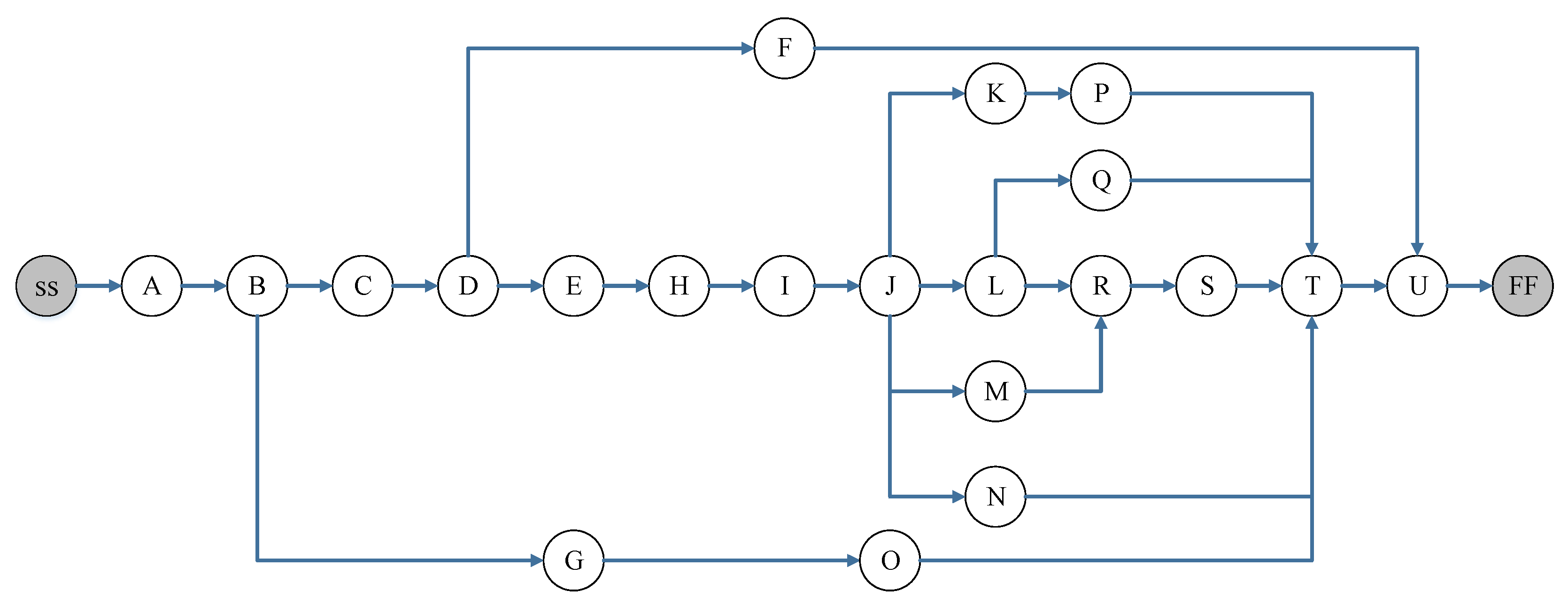
• An activity on node network with N activity is considered and the Nth activity is a dummy with zero duration.

3.1. Proposed Model

Notations

Sets

$j=1, 2,\dots ,N$	Set of project activities
$t=1, 2,\dots ,T$	Set of time periods for project
$m=1, 2,\dots ,M_j$	A set of executive modes for project activity $j$
$k=1, 2,\dots ,K$	A set of renewable resources of the project
$i=1, 2,\dots ,I$	A set of non-renewable resources of the project
$p\left(j^{\prime },j\right)$	Set the precedence relationships between project activities

Parameters

$dd$	Specified due dates for the project
$tb$	Total budget for renewable and non-renewable resources
$c{r}_k$	Cost of renewable resource unit $k$
$c{w}_i$	Cost of non-renewable resource unit $i$
$E{F}_j$	Earliest finish time of activity $j$
$L{F}_j$	Latest finish time of activity j
$d_{jm}^e$	Duration of activity j in the executive mode m in the crashing way
$d_{jm}^n$	Duration of activity $j$ in the executive mode $m$ in the normal way
$Q_{jm}^e$	Quality of activity $j$ in the executive mode $m$ in the crashing way
$Q_{jm}^n$	Quality of activity $j$ in the executive mode $m$ in the normal way
$r_{jmk}^e$	Renewable resource k required for activity $j$, when performed in a crashing way on mode $m$
$r_{jmk}^n$	Renewable resource $k$ required for activity $j$, when performed in normal way and on mode $m$
$w_{jmi}$	Non-renewable resource $i$ required for the activity $j$, when performed on mode $m$
$M$	Big number
${\sigma }_{j^{\prime }}$	Standard deviation of activity duration $j^{\prime }$

Decision variables

$x_{jmt}$	$\{\begin{array}{c}1\\ 0\end{array}$	If activity $j$ is executed in mode $m$ and ends in time $t$  Otherwise
$Y_j$	$\{\begin{array}{c}1\\ 0\end{array}$	If activity $j$ is crashed  Otherwise
$bet{a}_{j^{\prime }}$	$\{\begin{array}{c}1\\ 0\end{array}$	If activity $j^{\prime }$ is floating  Otherwise
$B{R}_k$	The amount of renewable resource $k$ allocated to the project
$B{W}_i$	The amount of non-renewable resource $i$ allocated to the project
$Tc$	The amount of time delay of the project
$alf{a}_{j^{\prime }}$	Related to the float of activity $j^{\prime }$
$ep{p}_{j^{\prime }}$	Amount of activity float $j^{\prime }$
$kk$	Project network complexity

3.2. Mathematical Model

The mathematical model for the scheduling construction projects is provided below:

$$z_1=min Tc+{\displaystyle \sum }_{j^{\prime }=1}^{N}bet{a}_{j^{\prime }}·KK·{\sigma }_{j^{\prime }}$$

(1)

$$z_2=max{\displaystyle \sum }_{j=1}^N{\displaystyle \sum }_{m\in M_j}{\displaystyle \sum }_{t=E{F}_j}^{L{F}_j}(Q_{jm}^e·Y_j·x_{jmt})+\left(Q_{jm}^n·x_{jmt}-Q_{jm}^n·x_{jmt}·Y_j\right)$$

(2)

Subject to:

$${\displaystyle \sum }_{m\in M_j}{\displaystyle \sum }_{t=E{F}_j}^{L{F}_j}{x}_{jmt}=1;\forall j\in N$$

(3)

$$\begin{gathered} {\displaystyle \sum }_{m\in M_j}{\displaystyle \sum }_{t=E{F}_j}^{L{F}_j}\left(t·x_{jmt}-\left(\left(d_{jm}^e·Y_j·x_{jmt}\right)+\left(d_{jm}^n·x_{jmt}-d_{jm}^n·Y_j·x_{jmt}\right)\right)\right) \\ \ge {\displaystyle \sum }_{m\in M_{j^{\prime }}}{\displaystyle \sum }_{t=E{F}_{j^{\prime }}}^{L{F}_{j^{\prime }}}t·x_{j^{\prime }mt};\forall \left(j^{\prime },j\right)\in p \end{gathered}$$

(4)

$$\begin{gathered} {\displaystyle \sum }_{j=1}^N{\displaystyle \sum }_{m\in M_j}{\displaystyle \sum }_{q=max\left\{t,E{F}_j\right\}}^{min\left\{t+d_{jm}^n-1,L{F}_j\right\}}\left(Y_j·x_{jmq}·r_{jkm}^e\right)+\left(r_{jkm}^n·x_{jmq}-Y_j·x_{jmq}·r_{jkm}^n\right) \\ \le B{R}_k;\forall k\in K, t\in T \end{gathered}$$

(5)

$${\displaystyle \sum }_{j=1}^N{\displaystyle \sum }_{m\in M_{\dot{J}}}{\displaystyle \sum }_{t=E{F}_j}^{L{F}_j}{w}_{jim}·x_{jmt}\le B{W}_i;\forall i\in I$$

(6)

$${\displaystyle \sum }_{i\in I}c{w}_i·B{W}_i+{\displaystyle \sum }_{k\in K}c{r}_k·B{R}_k\le tb$$

(7)

$$Tc\ge {\displaystyle \sum }_{t=E{F}_N}^{L{F}_N}{\displaystyle \sum }_{m\in M_j}\left(t·x_{Nmt}-dd\right)$$

(8)

$$\begin{gathered} {\displaystyle \sum }_{m\in M_{\dot{J}}}{\displaystyle \sum }_{t=E{F}_j}^{L{F}_j}\left(t·x_{jmt}-\left(\right(d_{jm}^e·Y_j·x_{jmt})+(d_{jm}^n·x_{jmt}-d_{jm}^n·Y_j·x_{jmt}\left)\right)\right) \\ -{\displaystyle \sum }_{m\in M_{j^{\prime }}}{\displaystyle \sum }_{t=E{F}_{j^{\prime }}}^{L{F}_{j^{\prime }}}(\left(d_{j^{\prime }m}^e·Y_{j^{\prime }}·x_{j^{\prime }mt}\right)+(d_{j^{\prime }m}^n·x_{j^{\prime }mt}-d_{j^{\prime }m}^n·Y_{j^{\prime }}·x_{j^{\prime }mt}))=alf{a}_{j^{\prime }};\forall \left(j^{\prime },j\right)\in p \end{gathered}$$

(9)

$$\begin{gathered} alf{a}_{j^{\prime }}-{\displaystyle \sum }_{m\in M_{j^{\prime }}}{\displaystyle \sum }_{t=E{F}_{j^{\prime }}}^{L{F}_{j^{\prime }}}\left(t·x_{j^{\prime }mt}-\left(\left(d_{j^{\prime }m}^e·Y_{j^{\prime }}·x_{j^{\prime }mt}\right)+\left(d_{j^{\prime }m}^n·x_{j^{\prime }mt}-d_{j^{\prime }m}^n·Y_{j^{\prime }}·x_{j^{\prime }mt}\right)\right)\right) \\ =ep{p}_{j^{\prime }};\forall j^{\prime } \end{gathered}$$

(10)

$$ep{p}_{j^{\prime }}\le M·\left(1-bet{a}_{j^{\prime }}\right);\forall j^{\prime }$$

(11)

$$ep{p}_{j^{\prime }}\ge 1-bet{a}_{j^{\prime }},;\forall j^{\prime }$$

(12)

$$\left(kk-1\right)·{\displaystyle \sum }_{j^{\prime }=1}^{N}bet{a}_{j^{\prime }}={\displaystyle \sum }_{j^{\prime }=1}^{N-1}{\displaystyle \sum }_{j=2}^{N}p\left(j^{\prime },j\right)·bet{a}_{j^{\prime }}·bet{a}_j$$

(13)

$$bet{a}_{j^{\prime }},x_{jmt},Y_j\in \left\{0,1\right\}, alf{a}_{j^{\prime }}, ep{p}_{j^{\prime }},Tc,kk\ge 0;\forall j,m,t$$

(14)

Equations (1) and (2) represent the objective functions of the proposed mathematical model. The first objective function minimizes the sum of delays, including the buffer size determined by the complexity of the project activity network and the time interval between the end time of the last activity and the specified due date. The second objective function of the model maximizes the project quality. Constraint (3) guarantees that each activity is scheduled only once. Constraint (4) represents the precedence relationships between project activities. Constraints (5) and (6) state the maximum utilization level for renewable and non-renewable resources, respectively. Constraint (7) guarantees that the total cost of providing renewable and non-renewable resources will not exceed the total project budget. Constraint (8) calculates the delay caused by the time interval between the end time of the last activity and the due date specified. Constraints (9) and (10) calculate the amount of each activity float. Constraints (11) and (12) determine the critical and non-critical activities. Constraint (13) calculates the network complexity.

3.3. Linearization

The proposed model is linearized due to the presence of the following nonlinear expressions $Y_j·x_{jmt},$ $bet{a}_{j^{\prime }}·bet{a}_j$ and $bet{a}_{j^{\prime }}·KK$.

The linearization starts with defining two binary variables $z_{jmt}$, $B_{j^{\prime }j}$ and a new continuous variable $h_{j^{\prime }}.$ Nine new constraints are added to the model to ensure the equality of $z_{jmt}$, $B_{j^{\prime }j}$ and $h_{j^{\prime }}$ with nonlinear expressions [34,35]. Nonlinear expressions $bet{a}_{j^{\prime }}.bet{a}_j$ and $bet{a}_{j^{\prime }}·KK$ are equivalent to the binary variable $B_{j^{\prime }j}$ and the continuous variable $h_{j^{\prime }}$, respectively, and as a result, Equations (1) and (13) are converted into Equations (15) and (16). Finally, Equations (17)–(22) are added to the model.

$$z_1=min Tc+{\displaystyle \sum }_{j^{\prime }=1}^N{h}_{j^{\prime }}·{\sigma }_{j^{\prime }}$$

(15)

$${\displaystyle \sum }_{j^{\prime }=1}^N{h}_{j^{\prime }}-{\displaystyle \sum }_{j^{\prime }=1}^{N}bet{a}_{j^{\prime }}={\displaystyle \sum }_{j^{\prime }=1}^{N-1}{\displaystyle \sum }_{j=2}^{N}p\left(j^{\prime },j\right)·B_{j^{\prime }j}$$

(16)

$$h_{j^{\prime }}\le kk;\forall j^{\prime }$$

(17)

$$h_{j^{\prime }}\le M·bet{a}_{j^{\prime }};\forall j^{\prime }$$

(18)

$$h_{j^{\prime }}\ge kk-M·\left(1-bet{a}_{j^{\prime }}\right);\forall j^{\prime }$$

(19)

$$B_{j^{\prime }j}\le bet{a}_{j^{\prime }};\forall \left(j^{\prime },j\right)\in p$$

(20)

$$B_{j^{\prime }j}\le bet{a}_j;\forall \left(j^{\prime },j\right)\in p$$

(21)

$$B_{j^{\prime }j}\ge bet{a}_{j^{\prime }}+bet{a}_j-1;\forall \left(j^{\prime },j\right)\in p$$

(22)

The nonlinear expression $Y_j·x_{jmt}$ is replaced by a binary variable $z_{jmt}$. As a result, Equations (2), (4), (5), (9) and (10) are converted into Equations (23)–(27). The constraints (28)–(30) are also added to the model.

$$z_2=max{\displaystyle \sum }_{j=1}^N{\displaystyle \sum }_{m\in M_j}{\displaystyle \sum }_{t=E{F}_j}^{L{F}_j}(Q_{jm}^e·z_{jmt})+\left(Q_{jm}^n·x_{jmt}-Q_{jm}^n·z_{jmt}\right)$$

(23)

Subject to:

$$\begin{gathered} {\displaystyle \sum }_{m\in M_j}{\displaystyle \sum }_{t=E{F}_j}^{L{F}_j}\left(t·x_{jmt}-\left(\left(d_{jm}^e·z_{jmt}\right)+\left(d_{jm}^n·x_{jmt}-d_{jm}^n·z_{jmt}\right)\right)\right) \\ \ge {\displaystyle \sum }_{m\in M_{j^{\prime }}}{\displaystyle \sum }_{t=E{F}_{j^{\prime }}}^{L{F}_{j^{\prime }}}t·x_{j^{\prime }mt};\forall \left(j^{\prime },j\right)\in p \end{gathered}$$

(24)

$${\displaystyle \sum }_{j=1}^N{\displaystyle \sum }_{m\in M_j}{\displaystyle \sum }_{q=max\left\{t,E{F}_j\right\}}^{min\left\{t+d_{jm}^n-1,L{F}_j\right\}}\left(r_{jkm}^e·z_{jmq}\right)+\left(r_{jkm}^n·x_{jmq}-z_{jmq}·r_{jkm}^n\right)\le B{R}_k;\forall k\in K, t\in T$$

(25)

$$\begin{gathered} {\displaystyle \sum }_{m\in M_{\dot{J}}}{\displaystyle \sum }_{t=E{F}_j}^{L{F}_j}\left(t·x_{jmt}-\left(\right(d_{jm}^e·Z_{jmt})+(d_{jm}^n·x_{jmt}-d_{jm}^n·Z_{jmt}\left)\right)\right) \\ -{\displaystyle \sum }_{m\in M_{j^{\prime }}}{\displaystyle \sum }_{t=E{F}_{j^{\prime }}}^{L{F}_{j^{\prime }}}(\left(d_{j^{\prime }m}^e·Z_{j^{\prime }mt}\right)+(d_{j^{\prime }m}^n·x_{j^{\prime }mt}-d_{j^{\prime }m}^n·Z_{j^{\prime }mt}))=alf{a}_{j^{\prime }};\forall \left(j^{\prime },j\right)\in p \end{gathered}$$

(26)

$$\begin{gathered} alf{a}_{j^{\prime }}-{\displaystyle \sum }_{m\in M_{j^{\prime }}}{\displaystyle \sum }_{t=E{F}_{j^{\prime }}}^{L{F}_{j^{\prime }}}\left(t·x_{j^{\prime }mt}-\left(\left(d_{j^{\prime }m}^e·z_{j^{\prime }mt}\right)+\left(d_{j^{\prime }m}^n·x_{j^{\prime }mt}-d_{j^{\prime }m}^n·z_{j^{\prime }mt}\right)\right)\right) \\ =ep{p}_{j^{\prime }};\forall j^{\prime } \end{gathered}$$

(27)

$$z_{jmt}\le Y_j;\forall j,m,t$$

(28)

$$z_{jmt}\le x_{jmt};\forall j,m,t$$

(29)

$$z_{jmt}\ge x_{jmt}+Y_j-1;\forall j,m,t$$

(30)

4. Proposed Solution Methodology

The proposed solution methodology is presented in two steps under interval-valued fuzzy uncertainty. In the first step, the interval-valued fuzzy mathematical model is converted into a crisp equivalent model using the method of Jimenez et al. [22]. Then in the second step, the objective functions are optimized according to the multi-objective solution approach presented by Lin [23].

4.1. Step 1: The Crisp Equivalent Model

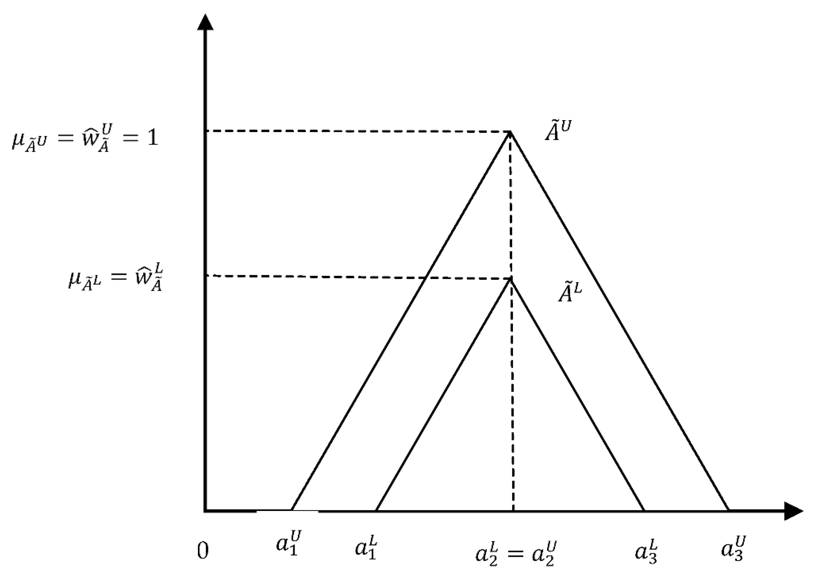
4.1.1. Triangular Interval-Valued Fuzzy Numbers

Given that the uncertainty lies in the duration of activities, and the lackness of historical data, the duration of each activity in this paper is expressed by normalized triangular interval-valued fuzzy numbers with numerous applications in complex management and engineering problems [36,37,38,39,40]. Interval-valued fuzzy sets theory is an extension made on fuzzy sets presented by Gorzalczany [41] in which an interval-valued fuzzy set has been defined at ($-\infty ,+\infty$) based on the following equations where ${\mu }_{{\tilde{A}}^L}\left(x\right)$ and ${\mu }_{{\tilde{A}}^U}\left(x\right)$ represent the lower and upper limits of membership functions, respectively:

$$\tilde{A}=\left\{x,\left[{\mu }_{{\tilde{A}}^L}\left(x\right),{\mu }_{{\tilde{A}}^U}\left(x\right)\right]\right\}, x \in \left(-\infty ,\infty \right), {\mu }_{{\tilde{A}}^L}, {\mu }_{{\tilde{A}}^U}: \left(-\infty ,\infty \right)\to \left[0, 1\right]$$

(31)

$${\mu }_{\tilde{A}}\left(x\right)=\left[ {\mu }_{{\tilde{A}}^L}\left(x\right),{\mu }_{{\tilde{A}}^U}\left(x\right)\right], {\mu }_{{\tilde{A}}^L}\left(x\right)\le {\mu }_{{\tilde{A}}^U}\left(x\right), \forall x \in \left(-\infty ,\infty \right),$$

(32)

Figure 1 illustrates a triangular interval-valued fuzzy number. Yao and Lin [42] also defined a triangular interval-valued fuzzy number as Equation (33), in which the lower and upper membership functions are displayed by ${\widehat{w}}_{\tilde{A}}^L={\mu }_{{\tilde{A}}^L}\left(x\right)$ and ${\mu }_{{\tilde{A}}^U}={\widehat{w}}_{\tilde{A}}^U$.

$$\tilde{A}=\left[{\tilde{A}}_x^L,{\tilde{A}}_x^U\right]=[\left(a_1^L,a_2^L,a_3^L;{\widehat{w}}_{\tilde{A}}^L\right),\left(a_1^U,a_2^U,a_3^U;{\widehat{w}}_{\tilde{A}}^U\right)]$$

(33)

In the above equation, ${\tilde{A}}^L$ and ${\tilde{A}}^U$ represent the lower and upper limits of the triangular interval-valued fuzzy numbers, respectively, where the following equation is established.

$${\tilde{A}}^L\subseteq {\tilde{A}}^U$$

(34)

Then, $\tilde{A}$ is a normalized triangular interval-valued fuzzy number which ${\mu }_{{\tilde{A}}^U}\left(x\right)={\mu }_{{\tilde{A}}^L}\left(x\right)$.

4.1.2. To Convert the Fuzzy Mathematical Model to a Crisp Equivalent Model

In this section, to de-fuzzy, the proposed model, the concepts and methods presented by Jimenez et al. [22] are discussed. This method enables the decision-maker to take into account the degree of aspiration level and the risk of constraints contravention within an interactive decision-making process [22]. According to the triangular fuzzy number $\tilde{A}=\left(a_1,a_2,a_3\right)$ and the corresponding membership function, which is expressed as follows:

$${\mu }_{\tilde{A}}=\{\begin{array}{cc}\begin{array}{c}\frac{x-a_1}{a_2-a_1}\end{array}\hfill & \hfill a_1\le x<a_2\\ 1\hfill & \hfill x=a_2\\ \frac{a_3^L-x}{a_3^L-a_2^L}\hfill & \hfill a_2\le x\le a_3\\ 0\hfill & \hfill x<a_1 or x>a_3\end{array}$$

(35)

Jimenez et al. [22] defined the expected value (EV) and expected interval (EI) for a triangular fuzzy number $\tilde{A}=\left(a_1,a_2,a_3\right)$ as Equations (36) and (37).

$$EV\left(\tilde{A}\right)=\frac{1}{4}\left(a_1+2a_2+a_3\right)$$

(36)

$$EI\left(\tilde{A}\right)=\left[E_1^A+E_2^A\right]=\left[\frac{1}{2}\left( a_1+a_2\right), \frac{1}{2}\left(a_2+a_3\right)\right]$$

(37)

Equation (38) represents a fuzzy mathematical model in which all the parameters of the problem are defined based on the triangular fuzzy numbers.

$$\begin{array}{c}min {\tilde{c}}^{T}X\\ \mathrm{Subject} \mathrm{to}:\\ {\tilde{a}}_i\ge {\tilde{b}}_i ;i=1,2,\dots ,l\\ {\tilde{a}}_i={\tilde{b}}_i ;i=l+1,\dots ,m\\ x\ge 0\end{array}$$

(38)

Therefore, taking into account the (EI), (EV) and $\alpha$ which is determined by the decision-maker as a feasibility degree of the model constraints, the crisp equivalent model is as follows:

$$\begin{array}{c}\min \left[EV\left({\tilde{c}}^T\right)\right]x\\ \mathrm{Subject} \mathrm{to}:\\ \left((1-\alpha \right)E_2^{a_i}+\alpha E_1^{a_i})x\ge \alpha E_2^{b_i}+\left(1-\alpha \right)E_1^{b_i};i=1,2,\dots ,l\\ \left(\left(1-\frac{\alpha }{2}\right)E_2^{a_i}+\frac{\alpha }{2}{E}_1^{a_i}\right)x\ge \frac{\alpha }{2}{E}_2^{b_i}+\left(1-\frac{\alpha }{2}\right)E_1^{b_i} ;i=l+1,\dots ,m\\ \left(\frac{\alpha }{2}{E}_2^{a_i}+\left(1-\frac{\alpha }{2}\right)E_1^{a_i}\right)x\le \left(1-\frac{\alpha }{2}\right)E_2^{b_i}+\frac{\alpha }{2}{E}_1^{b_i} ;i=l+1,\dots ,m\\ x\ge 0\end{array}$$

(39)

The proposed equivalent auxiliary crisp model is obtained by considering the concepts and relationships presented in Jimenez et al. [22] to present the duration parameters with triangular interval-valued fuzzy numbers; a crisp equivalent model is written for both the upper and lower limits. The equivalent model for the lower limit is as follows, which is the same for the upper limit.

$$z_1^L=min Tc+{\displaystyle \sum }_{j^{\prime }=1}^N{h}_{j^{\prime }}·{\sigma }_{j^{\prime }}$$

(40)

$$z_2^L=max{\displaystyle \sum }_{j=1}^N{\displaystyle \sum }_{m\in M_j}{\displaystyle \sum }_{t=E{F}_j}^{L{F}_j}(Q_{jm}^e·z_{jmt})+(Q_{jm}^n·x_{jmt}-Q_{jm}^n·z_{jmt})$$

(41)

$$\begin{gathered} {\displaystyle \sum }_{m\in M_j}{\displaystyle \sum }_{t=E{F}_j}^{L{F}_j}(t·x_{jmt}-((((1-\alpha )· E_2^{d_{jm}^{e^L}}+ \alpha ·E_1^{d_{jm}^{e^L}})·z_{jmt})+ \\ (((1-\alpha )· E_2^{d_{jm}^{n^L}}+ \alpha ·E_1^{d_{jm}^{n^L}})·(x_{jmt}-z_{jmt}))))\ge {\displaystyle \sum }_{m\in M_{j^{\prime }}}{\displaystyle \sum }_{t=E{F}_{j^{\prime }}}^{L{F}_{j^{\prime }}}t·x_{j^{\prime }mt};\forall (j^{\prime },j)\in p \end{gathered}$$

(42)

$${\displaystyle \sum }_{j=1}^N{\displaystyle \sum }_{m\in M_j}{\displaystyle \sum }_{q=\max \left\{t,E{F}_j\right\}}^{\min \{t+(\frac{d_{1jm}^{n^L}+2·d_{2jm}^{n^L}+d_{3jm}^{n^L}}{4})-1,L{F}_j\}}\left(r_{jkm}^e·z_{jmq}\right)+\left(r_{jkm}^n·x_{jmq}-z_{jmq}·r_{jkm}^n\right)\le B{R}_k;\forall k\in K, t\in T$$

(43)

$$\begin{gathered} {\displaystyle \sum }_{m\in M_j}{\displaystyle \sum }_{t=E{F}_j}^{L{F}_j}(t·x_{jmt}-((((1-\frac{\alpha }{2})· E_2^{d_{jm}^{e^L}}+(\frac{\alpha }{2})·E_1^{d_{jm}^{e^L}})·z_{jmt})+(((1-\frac{\alpha }{2})· E_2^{d_{jm}^{n^L}}+(\frac{\alpha }{2})·E_1^{d_{jm}^{n^L}})·(x_{jmt}-z_{jmt})))) \\ -{\displaystyle \sum }_{m\in M_{j^{\prime }}}{\displaystyle \sum }_{t=E{F}_{j^{\prime }}}^{L{F}_{j^{\prime }}}((((1-\frac{\alpha }{2})· E_2^{d_{jm}^{e^L}}+(\frac{\alpha }{2})·E_1^{d_{jm}^{e^L}})·z_{j^{\prime }mt})+(((1-\frac{\alpha }{2})· E_2^{d_{jm}^{n^L}}+(\frac{\alpha }{2})·E_1^{d_{jm}^{n^L}})·(x_{j^{\prime }mt}-z_{j^{\prime }mt})))\ge alf{a}_{j^{\prime }};\forall (j^{\prime },j)\in p \end{gathered}$$

(44)

$$\begin{gathered} {\displaystyle \sum }_{m\in M_j}{\displaystyle \sum }_{t=E{F}_j}^{L{F}_j}(t·x_{jmt}-((((\frac{\alpha }{2})· E_2^{d_{jm}^{e^L}}+(1-\frac{\alpha }{2})·E_1^{d_{jm}^{e^L}})·z_{jmt})+(((\frac{\alpha }{2})· E_2^{d_{jm}^{n^L}}+(1-\frac{\alpha }{2})·E_1^{d_{jm}^{n^L}})·(x_{jmt}-z_{jmt})))) \\ -{\displaystyle \sum }_{m\in M_{j^{\prime }}}{\displaystyle \sum }_{t=E{F}_{j^{\prime }}}^{L{F}_{j^{\prime }}}((((\frac{\alpha }{2})· E_2^{d_{jm}^{e^L}}+(1-\frac{\alpha }{2})·E_1^{d_{jm}^{e^L}})·z_{j^{\prime }mt})+(((\frac{\alpha }{2})· E_2^{d_{jm}^{n^L}}+(1-\frac{\alpha }{2})·E_1^{d_{jm}^{n^L}})·(x_{j^{\prime }mt}-z_{j^{\prime }mt})))\le alf{a}_{j^{\prime }};\forall (j^{\prime },j)\in p \end{gathered}$$

(45)

$$\begin{gathered} alf{a}_{j^{\prime }}-{\displaystyle \sum }_{m\in M_{j^{\prime }}}{\displaystyle \sum }_{t=E{F}_{j^{\prime }}}^{L{F}_{j^{\prime }}}(t·x_{j^{\prime }mt}-((((1-\frac{\alpha }{2})· E_2^{d_{j^{\prime }m}^{e^L}}+(\frac{\alpha }{2})·E_1^{d_{j^{\prime }m}^{e^L}})·z_{j^{\prime }mt})+ \\ (((1-\frac{\alpha }{2})· E_2^{d_{j^{\prime }m}^{n^L}}+(\frac{\alpha }{2})·E_1^{d_{j^{\prime }m}^{n^L}})·(x_{j^{\prime }mt}-z_{j^{\prime }mt}))))\ge ep{p}_{j^{\prime }};\forall j^{\prime } \end{gathered}$$

(46)

$$\begin{gathered} alf{a}_{j^{\prime }}-{\displaystyle \sum }_{m\in M_{j^{\prime }}}{\displaystyle \sum }_{t=E{F}_{j^{\prime }}}^{L{F}_{j^{\prime }}}(t·x_{j^{\prime }mt}-((((\frac{\alpha }{2})· E_2^{d_{j^{\prime }m}^{e^L}}+(1-\frac{\alpha }{2})·E_1^{d_{j^{\prime }m}^{e^L}})·z_{j^{\prime }mt})+ \\ (((\frac{\alpha }{2})· E_2^{d_{j^{\prime }m}^{n^L}}+(1-\frac{\alpha }{2})·E_1^{d_{j^{\prime }m}^{n^L}})·(x_{j^{\prime }mt}-z_{j^{\prime }mt}))))\le ep{p}_{j^{\prime }};\forall j^{\prime } \end{gathered}$$

(47)

4.2. Step 2: The Weighted Max–Min Model

To transform the proposed bi-objective model into a single-objective model, this paper uses the weighted max-min approach. The goal programming approach is utilized to solve the model according to the aspiration levels determined by the decision-maker. As it is not possible sometimes to accurately determine the aspiration level and also to present the different levels of importance for the delay and quality objective functions by the decision-maker, the fuzzy goal programming method has been suggested by Lin [23]. The ratio of the obtained levels should be as exact as possible to the ratio of the objective weights to show their relative importance [23].

A fuzzy goal programming problem is observed with m fuzzy goals according to Equation (48); $l_i$ represents the lower limit of the fuzzy goal ${\left(ax\right)}_i\tilde{\ge }{g}_i$.

$$\begin{array}{c}\mathrm{Find} x\\ \mathrm{to} \mathrm{satisfy} {\left(ax\right)}_i\tilde{\ge }{g}_i i=1, 2, \dots , m\\ \mathrm{Subject} \mathrm{to}:\\ Bx\le b\\ x\ge 0\end{array}$$

(48)

Therefore, the membership function of fuzzy goals ${\mu }_i^{\prime }\left({\left(ax\right)}_i\right)$ is stated as follows:

$${\mu }_i^{\prime }\left({\left(ax\right)}_i\right)=\frac{{\mu }_i\left({\left(ax\right)}_i\right)}{w_i}=\{\begin{array}{c}\frac{1}{w_i} \mathrm{if} g_i\le {\left(ax\right)}_i\\ \frac{f_i\left({\left(ax\right)}_i\right)}{w_i} \mathrm{if} l_i\le {\left(ax\right)}_i<g_i\\ 0 \mathrm{if} {\left(ax\right)}_i\le l_i\end{array}$$

(49)

$f_i\left({\left(ax\right)}_i\right)$ is a linear or piecewise linear membership function and $w_{i }$ is the relative weight of the objective function i. The weighted max-min approach is defined to solve multi-objective models with fuzzy goals according to Equation (50); $\lambda$ shows the optimal achieved level.

$$\begin{array}{c}\mathrm{Maximize} \lambda \\ \mathrm{Subject} \mathrm{to}:\\ w_i\lambda \le f_i\left({\left(ax\right)}_i\right) i=1,2,\dots ,m\\ w_i\lambda \le f_i\left({\left(ax\right)}_i\right) \\ x\ge 0\end{array}$$

(50)

In this paper, $l_i$ and $g_i$ obtained according to the positive $g_i^{\alpha -PIS}$ and negative $l_i^{\alpha -NIS}$ ideal solutions. After determining the ideal solutions, the membership function of Equation (49) is transformed into Equation (51).

$${\mu }_i^{\prime }\left({\left(ax\right)}_i\right)=\frac{{\mu }_i\left({\left(ax\right)}_i\right)}{w_i}=\{\begin{array}{c}\frac{1}{w_i} \mathrm{if} g_i^{\alpha -PIS}\le {\left(ax\right)}_i \\ \frac{f_i\left({\left(ax\right)}_i\right)}{w_i} \mathrm{if} l_i^{\alpha -NIS}\le {\left(ax\right)}_i<g_i^{\alpha -PIS}\\ 0 \mathrm{if} {\left(ax\right)}_i\le l_i^{\alpha -NIS} \end{array}$$

(51)

Finally, given that the duration of the activities is expressed using the triangular interval-valued fuzzy numbers, the weighted max-min model for lower limit membership functions is as follows:

$$\begin{array}{c}\mathrm{Maximize} {\lambda }^L\\ \mathrm{Subject} \mathrm{to}:\\ w_i{\lambda }^L\le \left(f_i({\left(ax\right)}_i\right){)}^L;i=1,2\end{array}$$

(52)

Due to the expansion of the feasible region for upper limits, it is expected to obtain better values for objective functions at the upper limit than at the lower limit. Therefore, Equations (53)–(55) are added to the model at the upper limit.

Maximize ${\lambda }^U$

Subject to:

$$w_i{\lambda }^U\le \left(f_i({\left(ax\right)}_i\right){)}^U;i=1,2$$

$$z_i^U\le z_i^L;i=1$$

(53)

$$z_i^U\ge z_i^L;i=2$$

(54)

$${\lambda }^U\ge {\lambda }^L$$

(55)

5. Case Study

In this section, a case study adapted from a study conducted by Ma et al. [1] is selected to validate the proposed model. A case study of a Tramway and related engineering systems project in a medium-sized city in China. The project network and the precedence relationships of the activities are shown in Figure 2. The network consists of 23 activities that are the start (ss) and end (ff) of the dummy activities of the network.

Project Information

The due date of the project by the employer is 180 days. Therefore, to minimize the delay in the project, activities should be performed as soon as possible. For each of the activities, two execution modes are defined in each of the normal and crashing execution ways. In addition, there is an available budget for resource costs of $8000, according to which the resources needed for the project, including personnel, machinery, and material, will be provided. The unit cost of personnel is $25 and $35 per machine. The unit cost of each material type (1) and (2) is $20 and $30, respectively.

6. Computational Results of the Case Study

The model is solved in GAMS software on a computer with 8 GB RAM and Cori5 CPU. The results of solving the mathematical model at the different levels of α and considering the equal weight by the employer for the two objective functions are displayed in

Table 1. Results of objective functions for upper limit.

$\mathit{\alpha }$	${\mathit{\mu }}_1^{\mathit{U}}$	${\mathit{\mu }}_2^{\mathit{U}}$	${\mathit{\lambda }}^{\mathit{U}}$	${\mathit{z}}_1^{\mathit{U}}$	${\mathit{z}}_2^{\mathit{U}}$	Buffer Size
0	0.947	0.944	1.888	3	0.987	3
0.1	0.949	0.946	1.892	2	0.987	2
0.2	0.925	0.925	1.851	3.022	0.987	3.022
0.3	0.927	0.933	1.853	3.18	0.989	3.18
0.4	0.937	0.936	1.872	3.538	0.989	1.538
0.5	0.947	0.949	1.894	2.36	0.989	2.36
0.6	0.942	0.941	1.883	2.9	0.989	2.9
0.7	0.952	0.944	1.888	1.84	0.987	1.84
0.8	0.97	0.966	1.932	1.68	0.993	1.68

. Due to the obtained solutions being better in the upper limit than in the lower limit, the results are presented only for the upper limit.

According to the results of alpha 0.1 given in Table 1, the value of the delay objective equals 2 days, which indicates that the project schedule is performed according to the specified due date and only predicts 2 buffer days for delays that may occur during execution. The value of the quality objective is also 0.987. It means that when both the objective functions are considered simultaneously, a number of activities are crashed, and the quality of the project is reduced to 0.987. As can be seen in the following equation, the ratio of the achieved levels of ${\mu }_1^U$ and ${\mu }_2^U$ are as exact as possible to the objective weights:

$$\frac{0.949}{0.5}\approx \frac{0.946}{0.5}\approx 1.892$$

(56)

At the alpha level of 0.2, the first objective function shows a delay of 3.022 days. In other words, the end time of the last activity in the schedule does not exceed the specified delivery date, and 3.022 buffer days are allowed for delays that may occur during execution. In addition, the quality objective function has not changed compared to the alpha level of 0.1, but the optimal achieved level has been reduced to 1.851. As another example, at the alpha level of 0.4, both objective functions are optimized with the obtained optimal achieved level of 1.872. In the first objective function, the end time of the last activity in the created schedule increases by 2 days compared to the specified due date, and 1.538 buffer days are predicted in the schedule. The quality objective represents the value of 0.989. If the first objective function is not considered and only the second objective function is presented in the model, the quality of the project equals 1. However, if both objective functions are considered simultaneously, a number of activities will be crashed, and the quality of the project will be reduced to 0.989. As can be seen in Table 1, by increasing $\alpha$, the objective function values do not follow a certain trend. It is also the project decision-maker who can choose the degree of achievability according to the values obtained for the project delay and quality.

7. Sensitivity Analysis

Here, to validate the proposed model, the results for the upper limit are compared under the following three conditions in

Table 2. The comparison of the results for the upper limit where $w_1=w_2=0.5$ and $\alpha =0.5$.

Activities Duration under Condition	${\mathit{\mu }}_1^{\mathit{U}}$	${\mathit{\mu }}_2^{\mathit{U}}$	${\mathit{\lambda }}^{\mathit{U}}$	${\mathit{z}}_1^{\mathit{U}}$	${\mathit{z}}_2^{\mathit{U}}$
1	0.947	0.949	1.894	2.36	0.989
2	0.93	0.928	1.855	2.688	0.989
3	0.738	0.738	1.476	29	0.929

:

• The duration of the activities is represented in the form of triangular interval-valued fuzzy numbers.
• The duration of the activities is expressed using the triangular fuzzy numbers.
• The duration of the activities is considered to be certain.

Under the three mentioned conditions, the model is solved using Lin [23] approach. When the duration of the activities is stated by triangular fuzzy numbers, the achieved optimal level and objective function values show better results than the duration of the activities being certain.

Thus, the comparison between the solutions of the model shows the better optimal achieved level and objective function values for which the duration of the activities is presented by the triangular interval-valued fuzzy numbers than the duration in the form of certain and triangular fuzzy numbers. In addition, the membership functions considering triangular interval-valued fuzzy numbers provide more desirable values due to the existence of equal weights for the two objective functions.

Crashing of activities is a process that reduces the project delay and increases costs (in this model, costs are expressed in terms of more resources). However, this process decreases the quality of activities, and consequently, the quality of the project. In

Table 3. Comparison between crashing and non-crashing activities.

	${\mathit{\mu }}_1^{\mathit{U}}$	${\mathit{\mu }}_2^{\mathit{U}}$	${\mathit{\lambda }}^{\mathit{U}}$	${\mathit{z}}_1^{\mathit{U}}$	${\mathit{z}}_2^{\mathit{U}}$
Crashing activities	0.947	0.949	1.894	2.36	0.989
Non crashing activities	0.873	0.916	1.746	7	0.993

, the proposed model is examined under the conditions of crashing activities and its absence. When the activities are crashed, the quality of the project is 0.989, and the corresponding delay is 2.36 days. Without crashing, the quality of the project is at the level of 0.993, and the corresponding delay is 7 days. Crashing has reduced the quality to a lower level than was not intended but has decreased the delay. Therefore, it can be concluded that the crashing of activities has improved the results of two objective functions at the same time.

8. Conclusions

Due to the factors that affect the timely completion of construction projects, a new bi-objective mathematical model is proposed in this paper, which aims to minimize the sum of delays and maximize the project quality to provide a schedule with construction project conditions using the critical chain method. In the proposed model, the renewable and non-renewable resource constraints, the calculation of buffer size based on network complexity, and activity duration presented by fuzzy numbers were considered. The solution process started with linearizing the nonlinear mathematical model. New proposed solution methodology was presented in two steps under interval-valued fuzzy uncertainty. The bi-objective model was aggregated using the weighted max-min approach presented by Lin [23] under three different conditions where the duration of activities was considered certain, triangular fuzzy numbers and triangular interval-valued fuzzy numbers. The model was validated by an adapted case study from the literature. The obtained results showed an upper optimal achieved level when the duration of the activities was stated as triangular interval-valued fuzzy numbers. It should be noted that the proposed approach is able to solve medium-sized projects in a short time. In cases where the size of the problem is large (mega projects), heuristics and meta-heuristics methods can be used as the solution time is greatly increased. This paper provides suggestions for developing and improving future research, such as applying group decision-making methods to determine duration parameters. Thus, with data obtained from several experts, the duration of activities can be determined. The mathematical model can also be developed by meta-heuristic and heuristic methods. Eventually, the human resources skills can be examined in executing project activities and evaluating them through the project delay and quality objective functions.

References

1. Ma, G.; Wang, A.; Li, N.; Gu, L.; Ai, Q. Improved critical chain project management framework for scheduling construction projects. J. Constr. Eng. Manag. 2014, 140, 04014055. [Google Scholar] [CrossRef]
2. Balta, S.; Birgonul, M.T.; Dikmen, I. Buffer sizing model incorporating fuzzy risk assessment: Case study on concrete gravity dam and hydroelectric power plant projects. ASCE-ASME J. Risk Uncertain. Eng. Syst. A Civ. Eng. 2018, 4, 04017039. [Google Scholar] [CrossRef]
3. Coelho, C.; Mojtahedi, M.; Kabirifar, K.; Yazdani, M. Influence of Organisational Culture on Total Quality Management Implementation in the Australian Construction Industry. Buildings 2022, 12, 496. [Google Scholar] [CrossRef]
4. Lapidus, A.; Topchiy, D.; Kuzmina, T.; Chapidze, O. Influence of the Construction Risks on the Cost and Duration of a Project. Buildings 2022, 12, 484. [Google Scholar] [CrossRef]
5. Fu, F.; Zhang, T. A new model for solving time-cost-quality trade-off problems in construction. PLoS ONE 2016, 11, e0167142. [Google Scholar] [CrossRef] [PubMed] [Green Version]
6. Hu, X.; Cui, N.; Demeulemeester, E.; Bie, L. Incorporation of activity sensitivity measures into buffer management to manage project schedule risk. Eur. J. Oper. Res. 2016, 249, 717–727. [Google Scholar] [CrossRef]
7. Hu, X.; Demeulemeester, E.; Cui, N.; Wang, J.; Tian, W. Improved critical chain buffer management framework considering resource costs and schedule stability. Flex. Serv. Manuf. J. 2017, 29, 159–183. [Google Scholar] [CrossRef]
8. Roghanian, E.; Alipour, M.; Rezaei, M. An improved fuzzy critical chain approach in order to face uncertainty in project scheduling. Int. J. Constr. Manag. 2018, 18, 1–13. [Google Scholar] [CrossRef]
9. Hall, N.G. Project management: Recent developments and research opportunities. J. Syst. Sci. Syst. Eng. 2012, 21, 129–143. [Google Scholar] [CrossRef]
10. Kastor, A.; Sirakoulis, K. The effectiveness of resource levelling tools for resource constraint project scheduling problem. Int. J. Proj. Manag. 2009, 27, 493–500. [Google Scholar] [CrossRef]
11. Watson, K.J.; Blackstone, J.H.; Gardiner, S.C. The evolution of a management philosophy: The theory of constraints. J. Oper. Manag. 2007, 25, 387–402. [Google Scholar] [CrossRef]
12. Ahlemann, F.; Arbi, F.E.; Kaiser, M.G.; Heck, A. A process framework for theoretically grounded prescriptive research in the project management field. Int. J. Proj. Manag. 2013, 31, 43–56. [Google Scholar] [CrossRef]
13. Rabbani, M.; Ghomi, S.F.; Jolai, F.; Lahiji, N.S. A new heuristic for resource-constrained project scheduling in stochastic networks using critical chain concept. Eur. J. Oper. Res. 2007, 176, 794–808. [Google Scholar] [CrossRef]
14. Tukel, O.I.; Rom, W.O.; Eksioglu, S.D. An investigation of buffer sizing techniques in critical chain scheduling. Eur. J. Oper. Res. 2006, 172, 401–416. [Google Scholar] [CrossRef]
15. She, B.; Chen, B.; Hall, N.G. Buffer sizing in critical chain project management by network decomposition. Omega. 2021, 102, 102382. [Google Scholar] [CrossRef]
16. Long, L.D.; Ohsato, A. Fuzzy critical chain method for project scheduling under resource constraints and uncertainty. Int. J. Proj. Manag. 2013, 31, 43–56. [Google Scholar] [CrossRef]
17. Mirnezami, S.A.; Mousavi, S.M.; Antuchevičienė, J.; Mohagheghi, V. A new approach for multi-scenario project cash flow analysis based on todim and critical chain methods under grey uncertainty. Econ. Comput. Econ. Cybern. Stud. Res. 2020, 54, 263–279. [Google Scholar]
18. Mirnezami, S.A.; Mousavi, S.M.; Mohagheghi, V. An innovative interval type-2 fuzzy approach for multi-scenario multi-project cash flow evaluation considering TODIM and critical chain with an application to energy sector. Neural. Comput. Appl. 2021, 33, 2263–2284. [Google Scholar] [CrossRef]
19. Atli, O.; Kahraman, C. Fuzzy resource-constrained project scheduling using taboo search algorithm. Int. J. Intell. Syst. 2012, 27, 873–907. [Google Scholar] [CrossRef]
20. Hajiagha, S.H.R.; Akrami, H.; Hashemi, S.S.; Mahdiraji, H.A. An integer grey goal programming for project time, cost and quality trade-off. Eng. Econ. 2015, 26, 93–100. [Google Scholar]
21. Albert, M.; Balve, P.; Spang, K. Evaluation of project success: A structured literature review. Int. J. Manag. Proj. Bus. 2017, 10, 796–821. [Google Scholar] [CrossRef]
22. Jiménez, M.; Arenas, M.; Bilbao, A.; Rodrı, M.V. Linear programming with fuzzy parameters: An interactive method resolution. Eur. J. Oper. Res. 2007, 177, 1599–1609. [Google Scholar] [CrossRef]
23. Lin, C.C. A weighted max–min model for fuzzy goal programming. Fuzzy Sets. Syst. 2004, 142, 407–420. [Google Scholar] [CrossRef]
24. Bie, L.; Cui, N.; Zhang, X. Buffer sizing approach with dependence assumption between activities in critical chain scheduling. Int. J. Prod. Res. 2012, 50, 7343–7356. [Google Scholar] [CrossRef]
25. Zhang, J.; Song, X.; Díaz, E. Project buffer sizing of a critical chain based on comprehensive resource tightness. Eur. J. Oper. Res. 2016, 248, 174–182. [Google Scholar] [CrossRef]
26. Zarghami, S.A.; Gunawan, I.; Corral de Zubielqui, G.; Baroudi, B. Incorporation of resource reliability into critical chain project management buffer sizing. Int. J. Prod. Res. 2020, 58, 6130–6144. [Google Scholar] [CrossRef]
27. Li, H.; Cao, Y.; Lin, Q.; Zhu, H. Data-driven project buffer sizing in critical chains. Autom. Constr. 2022, 135, 104134. [Google Scholar] [CrossRef]
28. Afruzi, E.N.; Najafi, A.A.; Roghanian, E.; Mazinani, M. A multi-objective imperialist competitive algorithm for solving discrete time, cost and quality trade-off problems with mode-identity and resource-constrained situations. Comput. Oper. Res. 2014, 50, 80–96. [Google Scholar] [CrossRef]
29. Tavana, M.; Abtahi, A.R.; Khalili-Damghani, K. A new multi-objective multi-mode model for solving preemptive time–cost–quality trade-off project scheduling problems. Expert Syst. Appl. 2014, 41, 1830–1846. [Google Scholar] [CrossRef]
30. Beşikci, U.; Bilge, Ü.; Ulusoy, G. Multi-mode resource constrained multi-project scheduling and resource portfolio problem. Eur. J. Oper. Res. 2015, 240, 22–31. [Google Scholar] [CrossRef] [Green Version]
31. Ashtiani, B.; Haghighirad, F.; Makui, A.; ali Montazer, G. Extension of fuzzy TOPSIS method based on interval-valued fuzzy sets. Appl. Soft Comput. 2009, 9, 457–461. [Google Scholar] [CrossRef]
32. Orm, M.B.; Jeunet, J. Time cost quality trade-off problems: A survey exploring the assessment of quality. CIE 2018, 118, 319–328. [Google Scholar] [CrossRef]
33. Mohammadipour, F.; Sadjadi, S.J. Project cost–quality–risk tradeoff analysis in a time-constrained problem. CIE 2016, 95, 111–121. [Google Scholar] [CrossRef]
34. Glover, F.; Woolsey, E. Converting the 0–1 polynomial programming problem to a 0–1 linear progra. Oper. Res. 1974, 22, 180–182. [Google Scholar] [CrossRef] [Green Version]
35. Norouzi, N.; Tavakkoli-Moghaddam, R.; Ghazanfari, M.; Alinaghian, M.; Salamatbakhsh, A. A new multi-objective competitive open vehicle routing problem solved by particle swarm optimization. Netw. Spat. Econ. 2012, 12, 609–633. [Google Scholar] [CrossRef]
36. Dorfeshan, Y.; Tavakkoli-Moghaddam, R.; Mousavi, S.M.; Vahedi-Nouri, B. A new weighted distance-based approximation methodology for flow shop scheduling group decisions under the interval-valued fuzzy processing time. Appl. Soft Comput. 2020, 91, 106248. [Google Scholar] [CrossRef]
37. Foroozesh, N.; Jolai, F.; Mousavi, S.M.; Karimi, B. A new fuzzy-stochastic compromise ratio approach for green supplier selection problem with interval-valued possibilistic statistical information. Neural. Comput. Appl. 2021, 33, 7893–7911. [Google Scholar] [CrossRef]
38. Foroozesh, N.; Tavakkoli-Moghaddam, R.; Mousavi, S.M. A novel group decision model based on mean–variance–skewness concepts and interval-valued fuzzy sets for a selection problem of the sustainable warehouse location under uncertainty. Neural Comput. Appl. 2018, 30, 3277–3293. [Google Scholar] [CrossRef]
39. Zolfaghari, S.; Mousavi, S.M. A novel mathematical programming model for multi-mode project portfolio selection and scheduling with flexible resources and due dates under interval-valued fuzzy random uncertainty. Expert Syst. Appl. 2021, 182, 115207. [Google Scholar] [CrossRef]
40. Patoghi, A.; Mousavi, S.M. A new approach for material ordering and multi-mode resource constraint project scheduling problem in a multi-site context under interval-valued fuzzy uncertainty. Technol. Forecast. Soc. Change 2021, 173, 121137. [Google Scholar] [CrossRef]
41. Gorzałczany, M.B. A method of inference in approximate reasoning based on interval-valued fuzzy sets. Fuzzy Sets. Syst. 1987, 21, 1–17. [Google Scholar] [CrossRef]
42. Yao, J.S.; Lin, F.T. Constructing a fuzzy flow-shop sequencing model based on statistical data. IJAR 2002, 29, 215–234. [Google Scholar] [CrossRef] [Green Version]
43. Kuo, M.S. A novel interval-valued fuzzy MCDM method for improving airlines’ service quality in Chinese cross-strait airlines. Transp. Res. Part E Logist. Transp. Rev. 2011, 47, 1177–1193. [Google Scholar] [CrossRef]
Figure 1. A triangular interval-valued fuzzy number A ˜ [43].
Buildings 12 00904 g001
Figure 2. Precedence relationships of activities in the node network [1].
Buildings 12 00904 g002