An Improved Model for Design Fatigue Load of Highway Bridges Considering Damage Equivalence

Abstract

Reasonable fatigue load should be determined before bridge fatigue analysis. However, the design frequency calculation method of the standard vehicle does not always make sense when the standard vehicle load model that is provided by existing standards is adopted, as the weights (equivalent coefficients) variation of different vehicle types are not considered from the perspective of damage equivalence. The method through direct damage calculation is workable but the process is usually laborious and time-consuming. To solve this problem, the traffic data of 35 highway sites involving 15 provinces in China were collected and the fatigue load spectrum were derived. The equivalent coefficients of each vehicle type at all of the 35 locations were calculated directly and the relationship with the corresponding gross vehicle weight was obtained formulaically through statistical analysis. Therefore, the design frequency of the standard vehicle can be calculated by the product of the actual frequency for a certain type of vehicle and the corresponding equivalent coefficient. The effectiveness of the proposed method was verified from the perspective of damage equivalence compared with the existing-standard method, and its flexibility and applicability for complex traffic conditions such as China were also demonstrated. In addition, three grades for the design frequency were put forward as references in relevant project design.

1. Introduction

Most steel structure failures are related to fatigue damage [1], and this is particularly prominent for steel bridges [2]. Take the orthotropic steel deck systems for example, fatigue cracks can often be found in a matter of years or decades of service as a result of the passing vehicles [3,4]. Generally, fatigue cracks are difficult to be noticed and repaired in the initial stage during the service period of steel structures [5], and the continuous propagation of fatigue cracks will affect the structural function and safety, and even cause bridge collapse accidents [6,7,8]. The realization of the durability goal of steel bridges (the design life of important bridges is usually 100 years or more) heavily depends on the solution of fatigue problems, and ‘fatigue durability’ is not a rare expression in the related literature [9,10]. Fatigue design or analysis is significant especially for steel bridges, with the premise of determining reasonable fatigue load. To ensure precise fatigue analysis and the achievement of bridge durability goals, a reasonable fatigue vehicle load model, which is also the focus in this paper, should be determined considering that the main variable load that is borne by highway bridges is vehicle load in engineering practice.

Presently, there are chiefly three forms of load model for fatigue analysis of bridges [11]: (a) fatigue load spectrum that is represented by several typical vehicles (short for “typical vehicle model”); (b) standard fatigue vehicle load model (short for “standard vehicle model”); (c) a vehicle that is used for standard live load in static strength design (short for “static model”). Specifically, among those mentioned models, the typical vehicle model is usually considered to be the closest to the actual fatigue load but not convenient for use, and “static model” is often considered to be inaccurate. The standard vehicle model is developed from the typical vehicle model based on the principle of damage equivalence. Considering the results and the solution procedures that are generated by this model that are capable of retaining certain accuracy and simplicity, it is widely accepted in fatigue analysis of bridges.

As shown in Figure 1, the standard vehicle model in China’s current design code of steel bridges [12] (denoted as Model III) is a four-axle vehicle with gross vehicle weight (GVW) of 48 t, which is similar to the Eurocode [13] except for simply modifying the ground contact dimensions of wheels. However, there are still several limitations of application with Model III for the actual traffic characteristics of China. As we know, China’s territory is approximately double that of the European Union (EU), and the overloading regulations [14,15], which has been proven to have significant influence on truck operating weights and may cause failure of the current fatigue load model [16], are different. Recently, Deng et al. [17] revealed that the fatigue damage that was calculated with Model III can large errors to emerge in several regions in China. Thus, it is necessary for the Model III to undertake more in-depth and comprehensive research to improve its applicability and feasibility.

Figure 1. Standard fatigue vehicle load model in China’s code (unit: m).

Precisely, the standard vehicle model is generally involved with a standard vehicle and corresponding frequency. The conventional single-vehicle-model scheme is usually utilized in the mainstream fatigue design codes around the world [12,13,18]. Generally, the standard vehicle is often a single vehicle and the frequency is directly determined by the flow of the effective vehicles whose fatigue contribution can’t be ignored directly. Theoretically, the biggest challenge for utilizing the single-vehicle-model scheme is the varied traffic characteristics due to the uneven development across domestic regions. For instance, according to Zhou et al. [19], it was found that the GVW of the standard vehicle are 51 t and 29 t for Shanxi Province and Fujian Province, respectively. Therefore, an obviously conservative standard vehicle is certain to be selected to avoid underestimating the actual fatigue loads in some regions [19,20,21]. In view of the limitations of the conventional single-vehicle-model scheme, Deng et al. [17] proposed a two-vehicle-model scheme with a three-axle vehicle and a four-axle vehicle. In detail, compared to the Model III, this scheme is verified to have better adaptability in complex traffic conditions with higher accuracy. However, the new scheme is far from ideal because it is more complex to used and may still underestimate the actual fatigue loads in some cases (the maximum relative errors were up to −26% [17]).

Actually, the method for determining the standard vehicle standard vehicle’s frequency is also a determinant factor to determine the final fatigue damage besides the vehicle configuration. Traditionally, the frequency of the standard vehicle is determined by directly counting the average daily traffic flow (ADTF) of effective vehicles without taking the differences of fatigue damage that is caused by varied vehicle types into account. Therefore, to overcome the limitation that results from such a traditional method, a new frequency calculation method will be developed in this paper that is based on fatigue damage equivalence while the single standard vehicle in Model III remains unchanged. According to the new frequency calculation method, during the frequency determining process, different weights will be assigned for corresponding vehicles based on fatigue damage equivalence when calculating the frequency of a standard vehicle. Specifically, in the proposed method, higher flexibility of the fatigue damage equivalence principle is considered and the simplicity of the form for Model III is also retained.

To conduct the research, firstly, the traffic data sources at 35 highway locations involving 15 provinces in China were collected through weigh-in-motion (WIM) systems or existing research, and the fatigue load spectrum of the corresponding locations were derived or obtained; Secondly, based on the linear cumulative damage theory [22,23,24], the fatigue damage of the typical representative vehicles for the 35 locations and the standard vehicle was calculated. After obtaining the equivalent coefficients, i.e., the ratio of fatigue damage between typical the representative vehicles and the standard fatigue vehicle, the mathematical relationship with the gross vehicle weight is given based on the statistical analysis. On this basis, the weight of each typical representative vehicle can be determined through equivalent coefficients when the frequency of the standard vehicle is calculated by using the method that is proposed in this paper. Compared with the methods of optimizing standard vehicle configuration in other literature or that is recommended in the existing standards, the method that is proposed is more flexible and applicable, especially for the situation of China, whose territory is vast and the traffic characteristics among regions are significantly different.

2. Fatigue Damage Theory

The fatigue damage equivalence criterion is the theoretical basis for the study of the bridge fatigue load model. In the following discussion, the derivation of fatigue load spectrum, the calculation of vehicle fatigue damage, and the definition of equivalent coefficient and equivalent heavy vehicle flow follow the unified fatigue damage theory [22,23,24,25,26]. The definition of fatigue damage is not unique [27], so it is necessary to explain it here.

The reference stress amplitude of structural details is set as $\Delta {\sigma }_i$, and the corresponding fatigue life is $N_i$. According to the S-N line approach [23] for welded structures, the relationship between the stress amplitude and fatigue life can be expressed by Formula (1).

$$N_i\cdot \Delta {\sigma }_i{}^m=C$$

(1)

where, m and C are constant related to the material. For steel structures, m = 3 is generally taken.

If $n_i$ is the actual number of cycles corresponding to $\Delta {\sigma }_i$, according to the linear cumulative damage theory (Miner’s rule) [23,27], the corresponding fatigue damage can be defined as:

$$D_i=\frac{n_i}{N_i}$$

(2)

When the variable amplitude loading is applied, the total fatigue damage is:

$$D={\displaystyle \sum D_i}={\displaystyle \sum \frac{n_i}{N_i}}=\frac{1}{C}\cdot {\displaystyle \sum n_i\Delta {\sigma }_i^3}$$

(3)

3. Traffic Data Collection and Preprocessing

Data of traffic load involving 3.9 million vehicles was collected via 47 WIM systems in toll stations of highways involving 20 provinces of China in late May, 2015 (14 days in total). The traffic data were collected, including the vehicle type, passing time, axle group type, GVW, axle load, and other information, was the sum of all lanes in the same direction; see Table 1. However, the axle type information of Beijing and 7 other provinces (No. 1 to 8) was not effectively obtained, thus the corresponding fatigue load spectrum could not be derived as the vehicles can be hard to classify.

Table 1. Locations for WIM information collection.

Location Number	Province	Expressway/ Toll Station	Location Number	Province	Expressway/ Toll Station
1	Beijing	G2/Dayangfang	11	Hunan	G4/Yanglousi
2	Gansu	G30/Ganshan	12-1	Hebei	G4/Jiyu
3-1	Guangxi	G72/Guixiang	12-2		G20/Jilu
3-2		G75/Guihai	12-3		G1/Jiliao
4-1	Jilin	G1/Lalinhe	13-1	Henan	G4/Anyangbei
4-2		G1/Wulihe	13-2		G 4/Yu’e
5-1	Liaoning	G11/Dalian	13-3		G36/Yuwan
5-2		G1/Maojiadian	13-4		G 40/Yushan
5-3		G1/Wanjia	14	Heilongjiang	G1/Lalinhe
6-1	Shanxi	G30/Chencang	15-1	Hubei	G4/Yu’e
6-2		G30/Tongguan	15-2		G4/Xiang’e
6-3		G20/Wangquan	16-1	Jiangsu	S26/Suhu
6-4		G20/Wubu	16-2		G25/Sulu
7-1	Sichuan	G85/Yujian	16-3		G4211/Suwan
7-2		G65/Sichuan	17	Jiangxi	G70/Xiongcun
7-3		G42/Lindian	18-1	Shandong	G15/Fushan
7-4		G76/Longnaquba	18-2		G20/Luji
7-5		G75/Sichuan	18-3		G15/Lusu
7-6		G93/Sichuan	19-1	Shanxi	G55/Deshengkou
8	Zhejiang	G104/Fenshuiguan	19-2		G20/Jundu
9-1	Fujian	G15/Minyue	19-3		G20/Jiuguan
9-2		G15/Minzhe	20-1	Chongqing	G75/Chongxihe
9-3		G70/Mingan	20-2		G75/Xiangxingshan
10	Guangdong	G4/Yuebei

Generally, the vehicles with very limited fatigue damage contribution were omitted directly to lessen the workload of traffic data processing and the rest vehicles were called effective vehicles. However, there seems no unified filtering criteria so far. The fatigue damage contribution of the vehicles with a GVW less than 3.0 t can be ignored directly, and this has been widely accepted [17,19,20,28,29]. However, the threshold raises up to 6 t in NCHRP Report [30], or 10 t in the Euro-code [13] and the Chinese code [12]. The frequency calculation is closely related to the definition of effective vehicles or filtering criterion. Thus, the vehicles were divided into three groups to facilitate discussion, that is “below 3 t”, “3 to 10 t”, and “above 10 t”, which were respectively tagged as “light vehicles”, “medium vehicles”, and “heavy vehicles”. In the following discussion on fatigue damage, the data of the light vehicles was omitted in traffic data preprocessing. However, whether medium vehicles can be omitted needs further discussion later for few related studies could be found.

The statistics showed that, as shown in Figure 2, the proportion of light vehicles and heavy vehicles varied greatly among the different locations that were under investigation, without obvious regularity. The proportion of medium vehicles was always low, with an average of about 8% and a maximum of 15.9%. However, as shown in Figure 3, the proportion of the “medium vehicles” was up to 35.8% (S26 Expressway located in Jiangsu Province, eastern China) after eliminating the light vehicles, and the values at half of the locations were more than 10%. Therefore, it made no sense to ignore the fatigue damage of medium vehicles from the perspective of traffic flow, only the data of light vehicles were omitted temporarily in the subsequent discussion.

Figure 2. Proportions of light vehicles, medium vehicles, and heavy vehicles.

Figure 3. Proportion of medium vehicles after excluding the light vehicles.

To facilitate the subsequent derivation of the fatigue load spectrum, the vehicles needed to be classified. Besides the GVM and axle number, the axle group type is also used as a basis for vehicle classification. Statistics show that the vast majority of the road vehicles can be categorized into 10 types based on the axle groups, namely “11”, “12”, “112”, “15”, “115”, “125”, “129”, “155”, and “1129”. The number “1” denotes single axle, single tire. The number “2” denotes single axle, double tires. The number “5” denotes tandem axles, double tires, and the number “9” denotes tridem axles, double tires. For the light vehicles and medium vehicles, vehicles of type “11” and “12” accounted for 98.0% and 96.4% by average, respectively, in the locations for the traffic data collection. For the heavy vehicles, 96.7% of the vehicles by average belonged to the 9 axle types: “12”, “112”, “15”, “115”, “125”, “129”, “155”, and “1129”. Therefore, it is reasonable to classify vehicles based on the 10 axle types. For a few of vehicles with axle types that were not included in Table 2, the corresponding vehicle flows were incorporated into the vehicle types with the same axle number in Table 2 in the following derivation process of fatigue load spectra. In addition, for the vehicles with more than 6 axles account for a very small proportion (no more than 1.4% in the locations surveyed) in the traffic flow of “heavy vehicles”, the vehicle flow was accumulated into the traffic flow of 6 axles.

Table 2. Vehicle classification in this paper.

Axle Number	Axle Type	Representative Axle Configuration	Representative Vehicle	GVW	Serial Number
2	11		small passenger car	3 t below	V1
	11		minivan (2 t below)		V2
	12		medium bus (11–30 seats)	3 to 10 t	V3
	12		medium truck (2–8 t)		V4
	12		Large bus (30 seats above)	10 t above	V5
	12		dual-axle large truck (8–16 t)		V6
3	112		large truck		V7
	15		large truck		V8
4	115		large truck		V9
	125		dual-axle tractor +dual-axle semi trailer		V10
5	129		dual-axle tractor +tri-axle semi trailer		V11
	155		tri-axle tractor +dual-axle semi trailer		V12
6	1129		tri-axle tractor +tri-axle semi trailer		V13
	159				V14

Thus, as shown in Table 2, the vehicles were categorized into 14 types (V1 to V14) in this paper based on comprehensive consideration of GVW, the axle number, and axle type. The description of the corresponding representative vehicle type refers to the investigation of typical vehicle models in China in reference [23].

4. Data of Fatigue Load Spectrum

4.1. Derivation of Fatigue Load Spectrum

The fatigue load spectrum is generally considered to be the closest form to the actual fatigue load, which can be used for the derivation of the standard fatigue vehicle load model and to judge the rationality of the proposed standard vehicle model. The fatigue load spectrum is composed of several typical representative vehicles and the corresponding frequency. Thus, the equivalent axle load, equivalent wheelbase, and the daily flow of each type of typical representative vehicle should be determined in a reasonable way.

The wheelbases for the typical representative vehicle type $V_i$ (i = 3 to 14) can usually be taken as the average value of the vehicles [20] of the same type. However, the collected vehicle data do not contain wheelbase data. As the wheelbase is fixed after leaving the factory and the variation range is small [20], the conclusion of the investigation on vehicle types in China by Wang et al. [31] was selected, and the unified wheelbase parameters of V3 to V14 are presented in Table 3.

Table 3. Wheelbases for the typical vehicle types.

Serial Number	Wheelbase (m)
	A1	A2	A3	A4	A5
V3	3.6
V4	3.8
V5	6
V6	5
V7	1.9	5.3
V8	4.8	1.3
V9	1.9	4.5	1.3
V10	3.5	8.6	1.3
V11	3.6	6.8	1.3	1.3
V12	3.3	1.3	6	1.3
V13	1.7	2.7	7.3	1.3	1.3
V14	3.3	1.3	9.3	1.3	1.3

Based on the principle of damage equivalence, the equivalent axle load of the typical representative vehicles in each location can be calculated by the Formula (4) [20]. The relevant data processing and calculation are completed by compiling VBA program. Due to space limitation, the calculation results of the equivalent axle load for each location are not presented in detail.

$$W_{ej}={(\frac{1}{N}{\displaystyle \sum _{i=1}^N{W}_{ij}^3})}^{1/3}$$

(4)

where $W_{ej}$ denotes the equivalent axle weight of the jth axle; $W_{ij}$ denotes the weight of the jth axle that is recorded by WIM system for the ith vehicle; and N denotes the number of vehicles in total of the same vehicle type.

Assuming that the equivalent GVW of the typical representative vehicle is the sum of each equivalent axle loads, the statistical results of the equivalent GVW for typical vehicles in the locations that were surveyed are shown in Table 4. It can be seen that the mean equivalent GVW of different vehicle types with the same axle number is relatively close and the dispersion of the equivalent GVW for the vehicles with more than three axles (V9 to V14) was relatively large on the whole according to the calculation results of variability coefficient.

Table 4. Statistical values of the equivalent GVW for each vehicle type(t).

	Statistical Values	Minimum	Maximum	Mean	Standard Deviation	Variability Coefficient
Serial Number
V3		5.1	8.4	7.0	0.9	0.13
V4		6.3	7.7	6.9	0.3	0.04
V5		14.4	18.3	16.2	0.8	0.05
V6		14.6	19.1	16.5	1.2	0.07
V7		19.3	28.8	24.2	2.2	0.09
V8		19.0	28.1	24.5	2.0	0.08
V9		27.2	43.6	34.3	3.8	0.11
V10		26.2	38.9	32.7	3.0	0.09
V11		32.9	47.9	42.2	3.8	0.09
V12		26.5	49.7	40.0	5.7	0.14
V13		33.2	60.2	48.5	6.4	0.13
V14		37.5	55.7	48.8	4.9	0.10

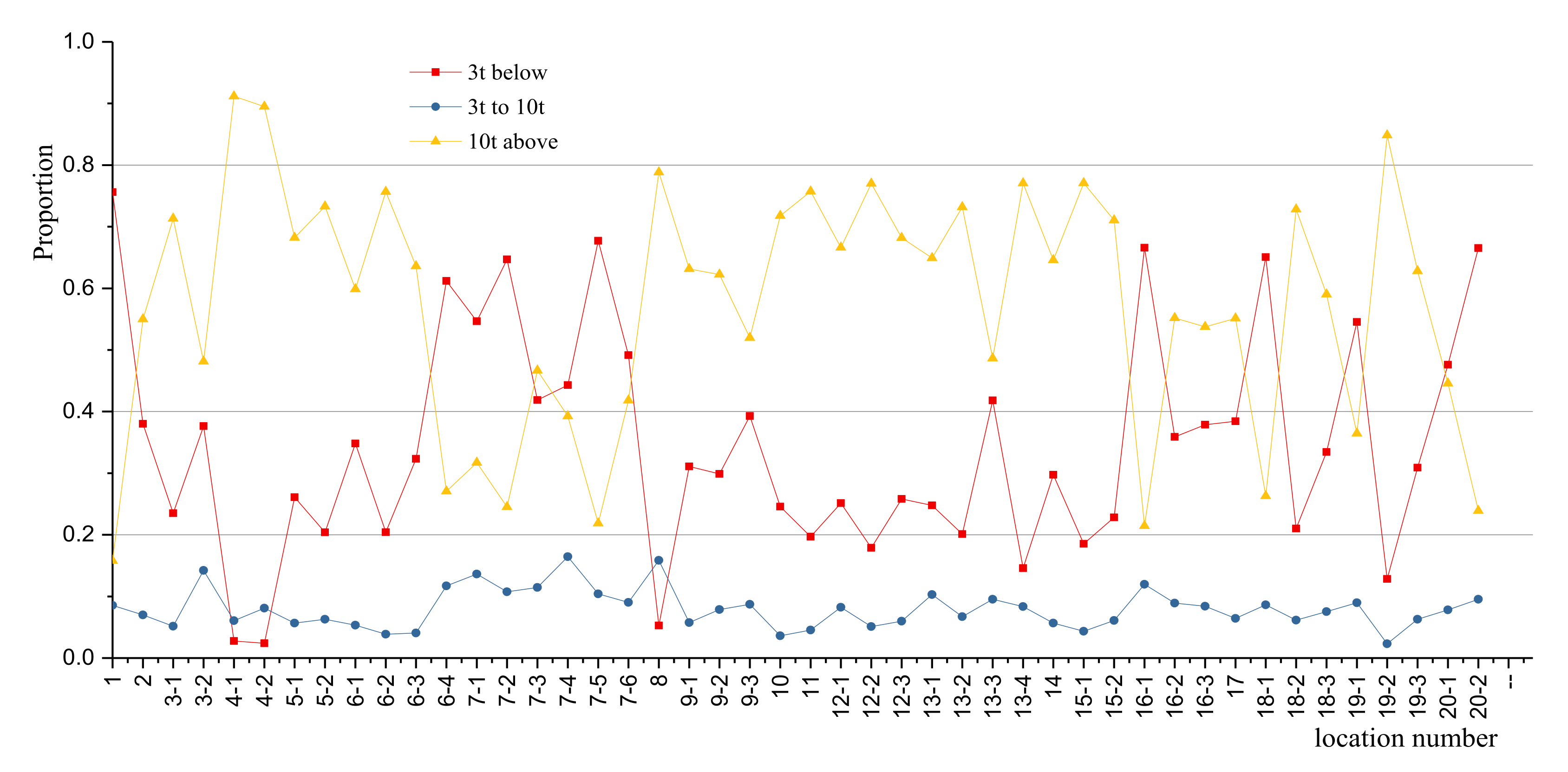
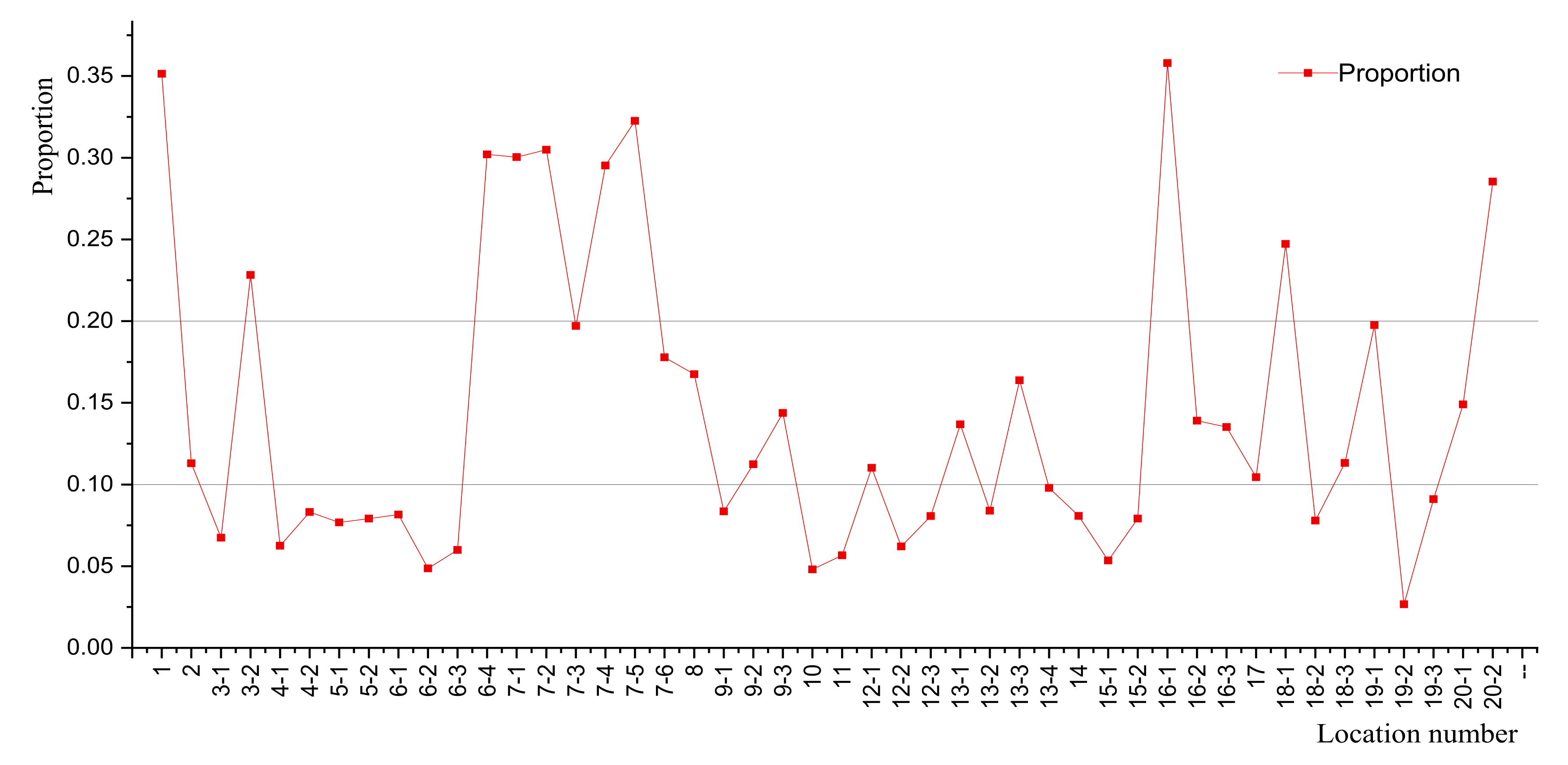
4.2. Lane Distribution Parameters

Generally, the composition of traffic flow in different lanes is different. The proportion of heavy vehicles in the slow lane is generally significantly higher than that in other lanes. On the other hand, the behaviors of fatigue vulnerable details of the bridge deck system, such as typical details of orthotropic steel deck (OSD) system [32], are mainly affected by the vehicle load of the lane in which it is located. Therefore, the fatigue damage near the slow lane is usually more serious in practical engineering and it is necessary to consider the distribution characteristics of the different vehicle types among lanes and the lane distribution parameters.

The recommended values of the lane distribution parameters are proposed in some of the literature [33,34,35] according to the field investigation. Based on that, the proportions of each typical representative vehicle type in the slow lane are summarized in Table 5. It should be noted that the recommended values in Table 4 are available only in normal situations while lacking of the reliable survey data, as the distribution parameters are also affected by some other factors. For example, drivers, even for heavy vehicles, tend to choose the inner lane for safe driving in the curved bridge lane with a large radian. The fatigue load spectrum of the slow lane can be obtained based on Table 5.

Table 5. Proportion of each typical vehicle type in the slow lane (%).

	Vehicle Type	2 Axles	3 Axles	4 Axles	5 Axles or More
Lanes
2-way 4-lane		70	100	100	100
2-way 6-lane		40	50	70	70
2-way 8-lane		25	45	60	65

4.3. Fatigue Load Spectrum of Slow Lane

According to the derivation method that is described in Section 4.1 and the lane distribution parameters in Table 5, the slow-lane fatigue load spectrum of the relevant investigation locations (No. 9 to 20, involving 27 locations in 12 provinces) was obtained. Limited by space, only the calculation results of the fatigue load spectra at location “15-1” are listed in Table 6. ADTF ($Q_{D,Vi}$, i = 3 to 12) in Table 6 denotes the average daily traffic flow in the slow lane.

Table 6. The fatigue load spectra of the slow lane at the location of ‘15-1′.

Vehicle Type	Equivalent Axle Load (t)						Equivalent	ADTF
	1st Axle	2nd Axle	3rd Axle	4th Axle	5th axle	6th Axle	GVW
V3	2.4	4.1					6.4	35
V4	2.7	4.5					7.2	147
V5	6.4	10.9					17.3	223
V6	5.3	11.8					17.1	221
V7	4.8	4.8	15.2				24.7	227
V8	6.5	10.6	10.6				27.8	51
V9	5.7	6.1	12.3	12.3			36.4	435
V10	4.7	11.6	10.1	10.1			36.4	83
V11	5.6	14.2	8.7	8.7	8.7		45.9	315
V12	5.6	8.8	8.8	12.9	12.9		48.9	14
V13	4.7	4.8	14.9	9.9	9.9	9.9	54.2	1366
V14	5.5	9.8	9.8	9.6	9.6	9.6	53.9	1376

Meanwhile, considering the limitations of the WIM data that were collected, the fatigue load spectrum at 8 typical locations in China were selected as a supplementary source to increase the coverage of the research data across the whole country, as shown in Table 7.

Table 7. Traffic data of eight typical locations from the public literature.

Location Number	Locations	Notes
21	Xinyihe bridge, Jiangsu province	Large bridge
22	Inner Mongolia section of G6 Expressway	Main channel for coal transportation
23	Jiujiang Yangtze River Bridge, on the boundary between Jiangxi Province and Hubei Province	Large bridge
24	Zhejiang province	Port highway
25	Pingsheng Bridge, Guangdong province	Large bridge
26	Guangxi province	Highway toll station
27	Guizhou province	Highway toll station
28	Humen Bridge, Guangdong province	Large bridge

Among the 8 locations, Xinyihe bridge (No. 21) [36], Jiujiang Yangtze River Bridge (No. 23) [37], Pingsheng Bridge (No. 25) [1], and the Humen Bridge (No. 28) [34] can reflect the traffic characteristics of large bridges in China. The Inner Mongolia section of G6 (No. 22) [38] is the main channel for Inner Mongolia coal transportation, which has the characteristics of large traffic flow, high proportion of lorries and heavy load. The port highway in Zhejiang province (No. 24) [39] reflects the transportation characteristics of port highway in China. The fatigue load spectra of the highway in Guangxi province (No. 26) [40] and Guizhou province (No. 27) [41] can, respectively, represent the traffic characteristics of the two provinces that were not involved in the WIM data that were collected.

Finally, the fatigue load spectrum of a total of 35 locations (No. 9 to 27) involving 15 provinces in China with 23 provinces in total were obtained for further analysis.

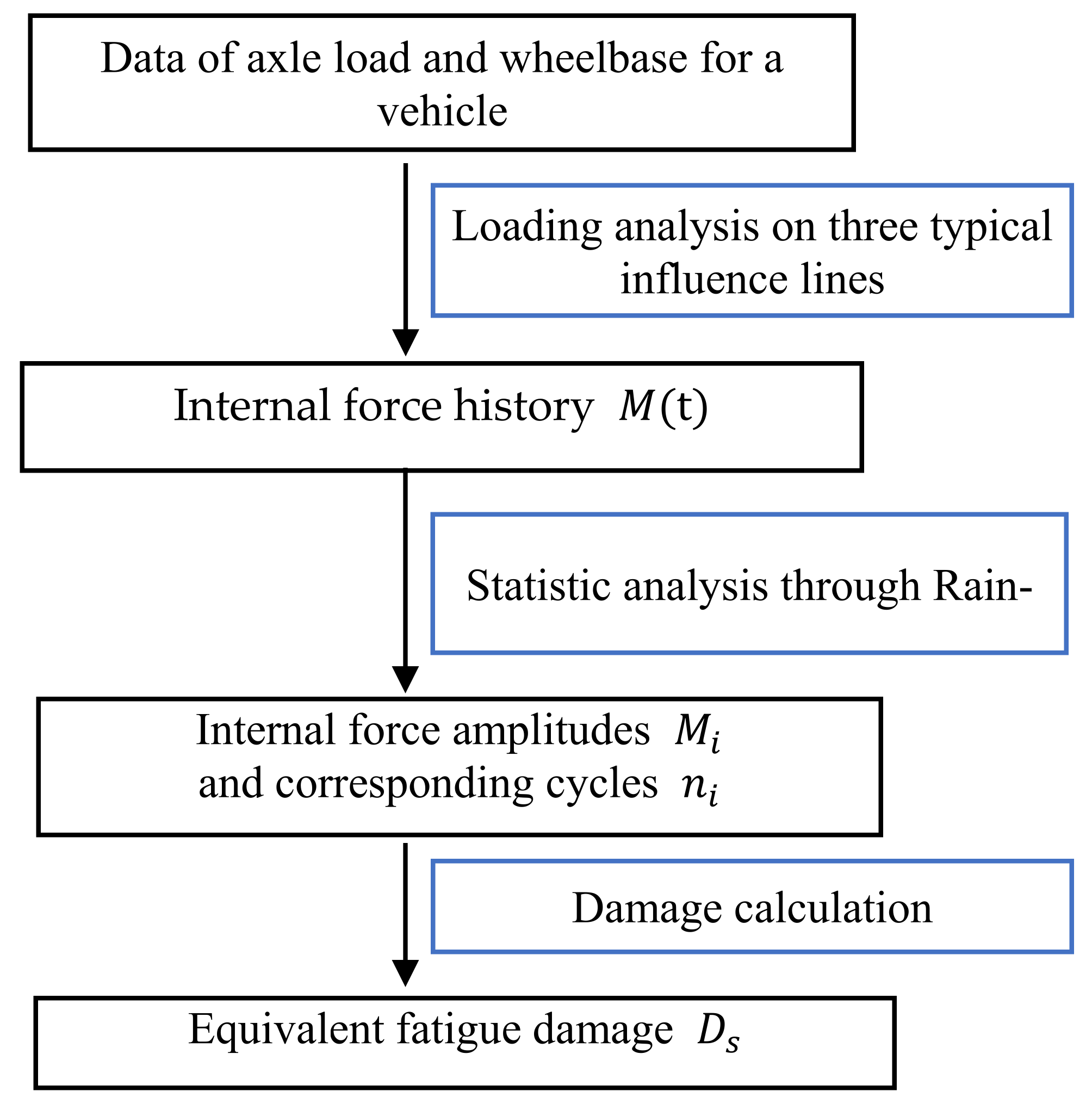
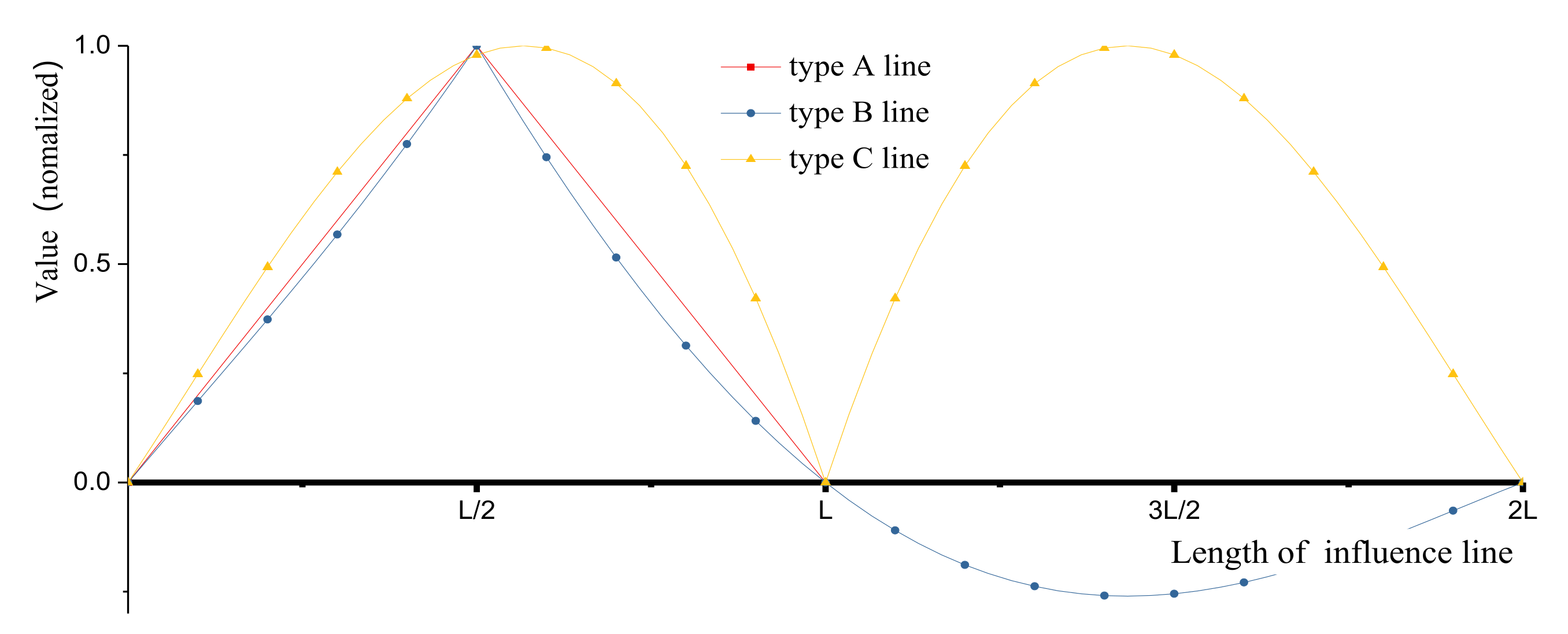
5. Fatigue Damage Calculation

The equivalent fatigue damage of the standard vehicle (JTG D64-2015) or a typical representative vehicle in the fatigue load spectra can be calculated according to the steps in Figure 4.

Figure 4. Calculation steps of fatigue damage.

Take the standard vehicle as an example.

Firstly, the section internal force (section moment) history of the vehicle is obtained by the influence line loading. For general consideration, there are three kinds of influence-line shapes [17], which, respectively, are the bending moments at three critical sections, namely the mid-span section of simply supported girder, the mid-span section, and the mid-support section of two equal-span continuous girder, and can be recorded as “type A line”, “type B line”, and “type C line”, as shown in Figure 5. The characteristic length of the influence lines (L) varies from 1m to 100 m (L= (1.0 1.2 1.5 2 3 4 5 6 7 8 9 10 11 12 14 15 16 18 19 20 30 50 75 100)).

Figure 5. Schematic diagram of the three types of influence lines (L: m).

Then, the bending moment history that is obtained by influence line loading is processed by the rain flow counting method [42] to obtain the bending-moment amplitudes $\Delta M_i$ and corresponding cycles $n_i$.

Finally, the equivalent fatigue damage (EFD) of the standard vehicle can be calculated according to the basic theory (Formula (3)) of the linear cumulative fatigue damage [22]

$$D_s=\frac{1}{C}\cdot {\displaystyle \sum n_i\cdot \Delta {\sigma }_i^3}=\frac{1}{C\cdot W}{\displaystyle \sum n_i\cdot \Delta M_i^3}=\frac{1}{W}\cdot D_0$$

(5)

where, $\Delta {\sigma }_i$ denotes the reference stress for a fatigue detail, W denotes section modulus, and $D_0$ is regarded as the relative equivalent fatigue damage (REFD) of the standard vehicle.

The section modulus W, which represents the section characteristic value, can generally be regarded as a constant when calculating the fatigue damage of a certain fatigue detail. Thus, the REFD can be used to replace EFD to denote the vehicle fatigue damage in the following discussion and the calculation of W can be avoided.

The calculation of REFD is completed by MATLAB (Version: 9.5.0). The relationship between the REFD of the standard vehicle ($D_0$) and the influence line is shown in the Figure 6, which indicates that:

Figure 6. The REFD values of the standard vehicle with varying influence lines.

(1)

the fatigue damage is not only affected by the shape of the influence line, but also closely related to the length;

(2)

the curve shows no regular pattern as the influence line length (L) is less than 30 m, while the REFD values seems to increase monotonously with ‘L’ increasing as ‘L’ exceeds 30 m and will basically close to an upper limit value when the length increases to 100 m.

The REFD values of the typical representative vehicles in the 35 locations were also calculated in this method. However, the details of the calculation results are not presented in detail for limitation of space.

Based on the calculation results, whether the fatigue damage contribution of medium vehicles should be considered in the fatigue analysis can be discussed here. According to the vehicle classification in Table 2, the medium vehicles include the vehicle types of “$V_3~V_4$”, and the heavy vehicles include the vehicle types of “$V_5~V_{14}$”. The ratio of fatigue damage of the medium vehicles ($D_{MV}$) to that of the heavy vehicles ($D_{HV}$) can be used as a criterion for judgment. Considering the length effect of the influence lines, the $D_{MV}/D_{HV}$ value is not a constant, therefore, the maximum value of $D_{MV}/D_{HV}$ was selected to be the representative value, which can be calculated according to the following formula:

$$\max \left\{D_{MV}/D_{HV}\right\}=\max \left\{{\displaystyle \sum _{i=3}^4(Q_{Vi}\cdot D_{Vi})}/{\displaystyle \sum _{j=5}^{14}(Q_{Vj}\cdot D_{Vj})}\right\}$$

(6)

where,$Q_{Vi}$,$Q_{Vj}$ denotes the average daily traffic flow of $V_i$, $V_j$; $D_{Vi}$, and $D_{Vj}$ denotes the REFD of a typical representative vehicle of $V_i$, $V_j$ in a certain location.

The calculation results are shown in Figure 7. It can be seen that the highest ratio of REFD was only 2.6% (location of “16-1”) while the ratio of the corresponding vehicle flow was 35.6%. So, it is reasonable to ignore the fatigue damage contribution of vehicles that were under 10 t in fatigue analysis.

Figure 7. Ratio of fatigue damage between the medium vehicles and the heavy vehicles.

6. Equivalent Coefficients and Equivalent Heavy Vehicle Flow

6.1. Equivalent Coefficients

The REFD value of a typical representative vehicle $Vi$ (i = 5 to 12) for a certain location is marked as $D_i$, then the equivalent coefficient (EC) of $Vi$ can be defined as

$${\delta }_{Vi}=D_{Vi}/D_0$$

(7)

EC reflects the relationship between the typical representative vehicle and the standard vehicle from the perspective of fatigue damage. ${\delta }_{Vi}=1$ means the fatigue damage of $Vi$ is equal to the standard vehicle, while the degree of deviation from 1 can reflect the difference of the fatigue damage between $Vi$ and the standard vehicle.

Take the location of “15-1” for example.

The calculated EC values (Vs “length of influence lines”) of partial typical vehicles are shown in Figure 8. It can be seen that the EC values of the same typical vehicle are dominated by the shape and length of the influence lines.

Figure 8. EC values vs. the influence lines at ‘15-1′.

The shapes of the influence lines seem to have less effect on EC values as the length if the influence line is more than 30 m, and the EC values of each typical representative vehicle change monotonously and tend gradually to a certain constant with the length of influence line increasing to 100 m. However, the EC curves that are affected by multiple factors seem to be irregular as the influence line length is less than 30 m. Therefore, the 30 m length can be regarded as a characteristic value to study the law of EC values.

For the convenience of analysis and discussion, three EC curves with different influence line shapes can be merged into one through extracting the maximum values. As shown in Figure 9, from which it can be found that each revised EC curve has two relatively significant peaks, which are approximately located in the intervals of 0 to 5 m and 5 to 30 m, as the length of the influence line is within 30 m. Therefore, the EC values for each typical representative vehicle can be divided into three groups according to the length of influence line: 5 m below (Group A), 5 to 30 m (Group B), and 30 m above (Group C).

Figure 9. The maximum EC values vs. the length of the influence line at “15-1”.

The maximum value of the EC values for $Vi$ in each group (denoted as ${{\delta }^{\prime }}_{Vi}$) can be selected to be the representative EC values. Thus, the representative EC values of $Vi$ in each group can be defined as

$${{\delta }^{\prime }}_{Vi}=\max \left\{{\delta }_{Vi}\right\}=\max \left\{D_{Vi}/D_0\right\}$$

(8)

In this way, the process of considering the effect of the influence lines on vehicle fatigue damage calculation can be greatly simplified.

The calculation results of the representative EC values for each typical representative vehicle in “15-1” are listed in Table 8. From which, it can be seen that the relative fatigue damage of different typical representative vehicles varies greatly. On the whole, the fatigue damage of the vehicles with three or less axles was generally lower than that of the standard vehicle, while the fatigue damage the vehicles with give or more axles was generally higher. Thus, the corresponding weight of each vehicle type should be reasonably considered when calculating the frequency of the standard fatigue.

Table 8. Representative EC values, ADTF, and EADTF of ‘15-1′.

Vehicle Type	Axle- Number	Representative EC Values			ADTF	EADTF
		5 m Below	5 to 30 m	30 m Above		5 m Below	5 to 30 m	30 m Above
V3	2	0.026	0.012	0.003	35	1	0	0
V4	2	0.034	0.017	0.005	147	5	2	1
V5	2	0.447	0.131	0.066	223	100	29	15
V6	2	0.514	0.202	0.074	221	114	45	16
V7	3	1.063	0.388	0.185	227	241	88	42
V8	3	0.781	0.817	0.31	51	40	42	16
V9	4	1.258	1.279	0.618	435	547	556	269
V10	4	0.907	0.7	0.41	83	75	58	34
V11	5	1.122	1.153	0.846	315	353	363	266
V12	5	1.459	1.211	1.04	14	20	17	15
V13	6	1.495	2.084	1.339	1366	2042	2847	1829
V14	6	1.725	2.53	1.23	1376	2374	3481	1692

6.2. Equivalent Average Daily Traffic Flow

According to the previous discussion, the effective vehicle means a vehicle with a GVW of more than 10 t. Thus, the average daily fatigue damage in a location based on the related specification ($D_D$) can be calculated as follows:

$$D_D=D_0\cdot {\displaystyle \sum _{i=5}^{14}{Q}_{D,Vi}}=D_0\cdot Q_D$$

(9)

where, $Q_D$ denotes the average daily traffic flow of the effective vehicles (ADTF).

While the average daily fatigue damage at a location based on the fatigue damage equivalence principle ($D_E$) can be calculated as follows:

$$D_E={\displaystyle \sum _5^{14}(D_{Vi}\cdot Q_{D,Vi})}=D_0\cdot {\displaystyle \sum _5^{14}({\delta }_{Vi}\cdot Q_{D,Vi}})$$

(10)

${{\delta }^{\prime }}_{Vi}$ is used to replace ${\delta }_{Vi}$ when the process of considering the effect of the influence lines is simplified based on the discussion in Section 6.1:

$$D_E\approx D_0\cdot {\displaystyle \sum _5^{14}({{\delta }^{\prime }}_{Vi}\cdot Q_{D,Vi}})=D_0\cdot {\displaystyle \sum _5^{14}{Q}_{E,Vi}}=D_0\cdot Q_E$$

(11)

The equivalent average daily traffic flow (EADTF, denoted as $Q_E$) can be defined as the product of the representative EC values and ADTF of the effective vehicles in the slow lane. The calculation result of ADTF and EADTF at location “15-1” is shown in Table 6.

EADTF, based on the consideration of fatigue damage equivalence is obviously more reasonable than ADTF. To explore the difference between EADTF and ADTF, the values of $Q_D/Q_E$ for all the locations that were surveyed were taken for research. As shown in Figure 10, it can be seen that: (1) when the length of the influence line is less than 5 m, the values corresponding about 40% locations surveyed less than 0.9; (2) when the length of the influence line is 5 to 30 m, the values corresponding about 43% locations surveyed less than 0.9; (3) when the length of the influence line exceeds 30 m, the values at all locations exceed 0.9. It indicates that it is likely to underestimate the fatigue load when the frequency of the standard vehicle is determined based on the ADTF that is recommended in the specification and the length of the influence line is within 30 m. However, the frequency of the standard vehicle based on ADTF is more likely to overestimate the fatigue load as the length of the influence line exceeds 30 m. On the other hand, the data show significant dispersion, ranging from 0.5 to 2.9. Therefore, the method to determine the frequency of the standard vehicle based on ADTF is not suitable for use from the perspective of fatigue damage equivalence.

Figure 10. $Q_D/Q_E$ at different locations.

Through analysis, the main reasons for the deviation between EADTF and ADTF are as follows: (1) The composition of the vehicle flow is not considered when the frequency of the standard vehicle is determined. The fatigue load is likely to be underestimated when the proportion of the vehicles with representative EC values that are larger than$1$ in traffic flow is high. (2) Possible overloading problems that are related to the local traffic management level and freight characteristics is not considered properly. Take the Inner Mongolia section of the G6 expressway for example. Traffic survey shows that the proportion of six-axle freight vehicles is as high as 76% and the overload phenomenon is serious, the maximal representative EC value of six-axle vehicles is as high as 4.1 (generally about 2.0). The fatigue load here will be seriously underestimated if ADTF is used according to the specification.

Therefore, the concept of EADTF should be adopted to replace ADTF in the standard vehicle frequency calculation, especially in the fatigue analysis of orthotropic steel deck (OSD) system for the influence line length of the fatigue details is generally within 30 m.

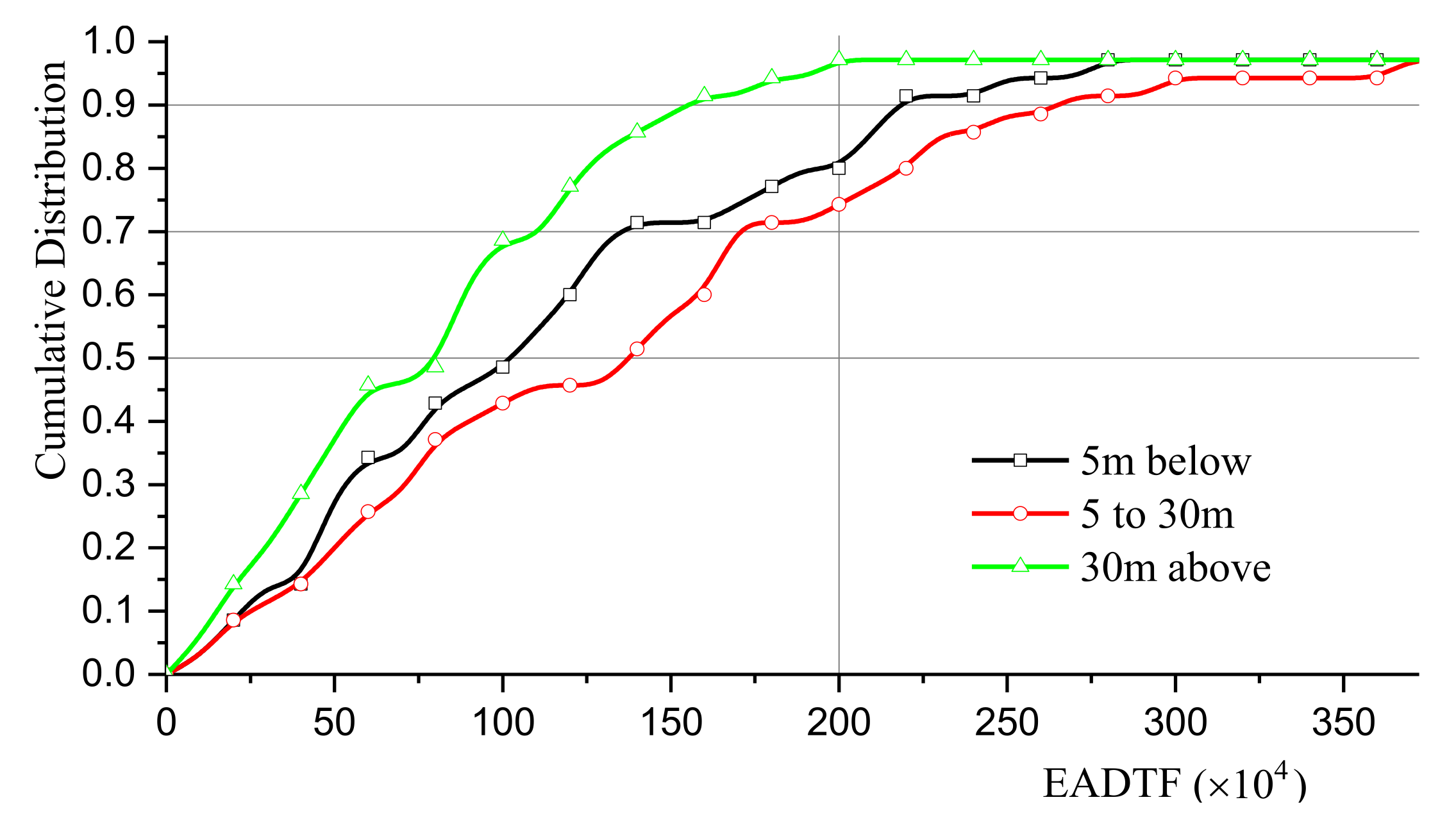
7. Determination for Design Frequency

According to the previous discussion, the design frequency of the standard vehicle can be determined by the EADTF of the typical representative vehicles other than ADTF. The key to calculating EADTF is calculating the representative EC values (${{\delta }^{\prime }}_{Vi}$). However, a simple and practical calculation method for determining the representative EC values needs to be developed.

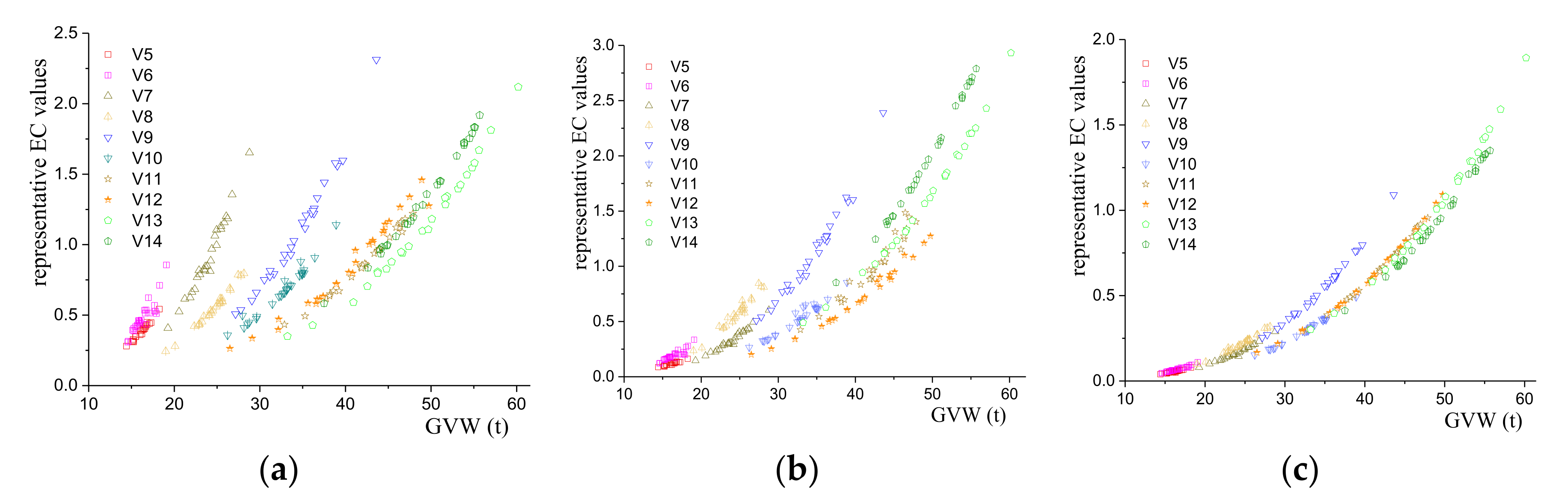
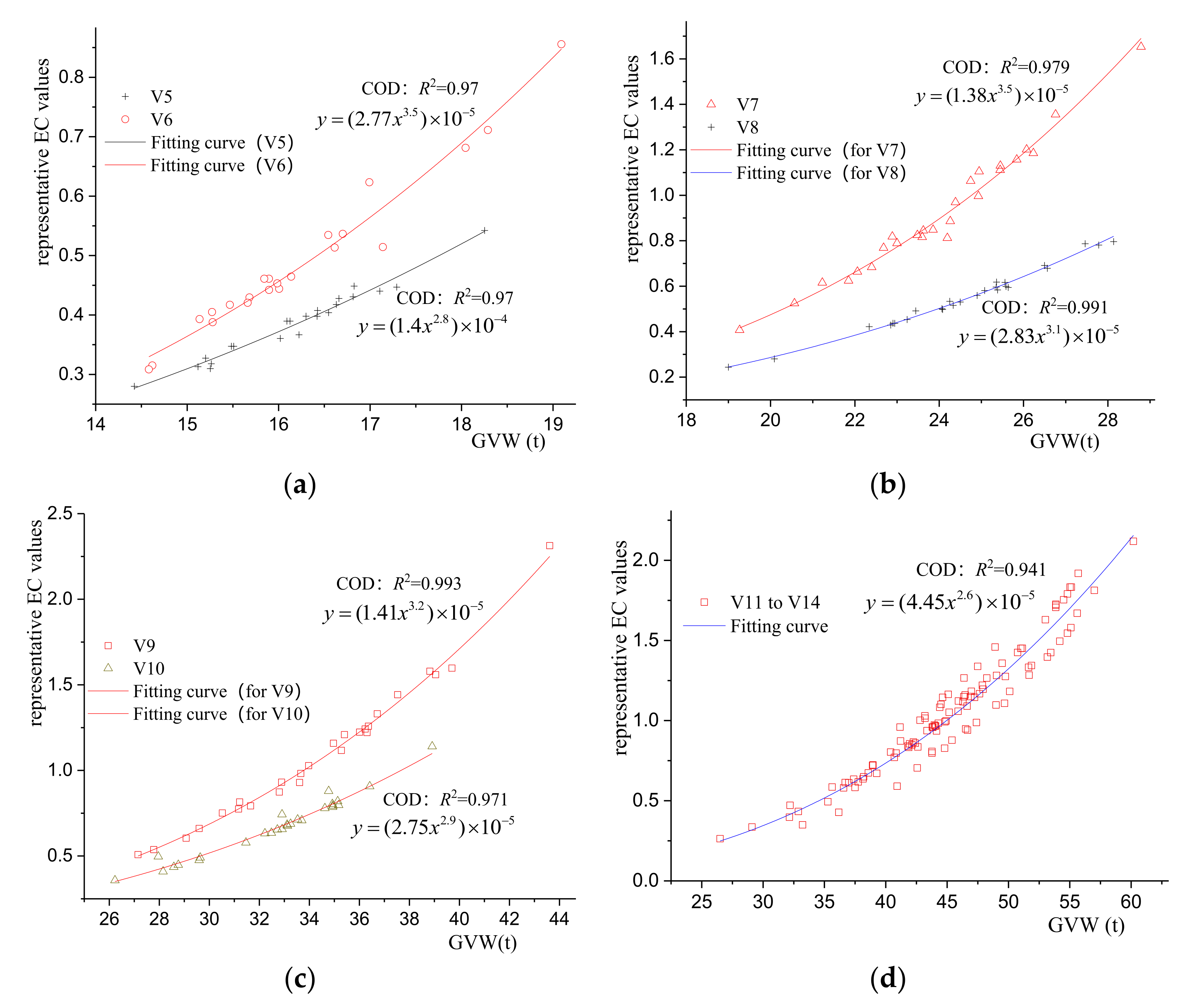
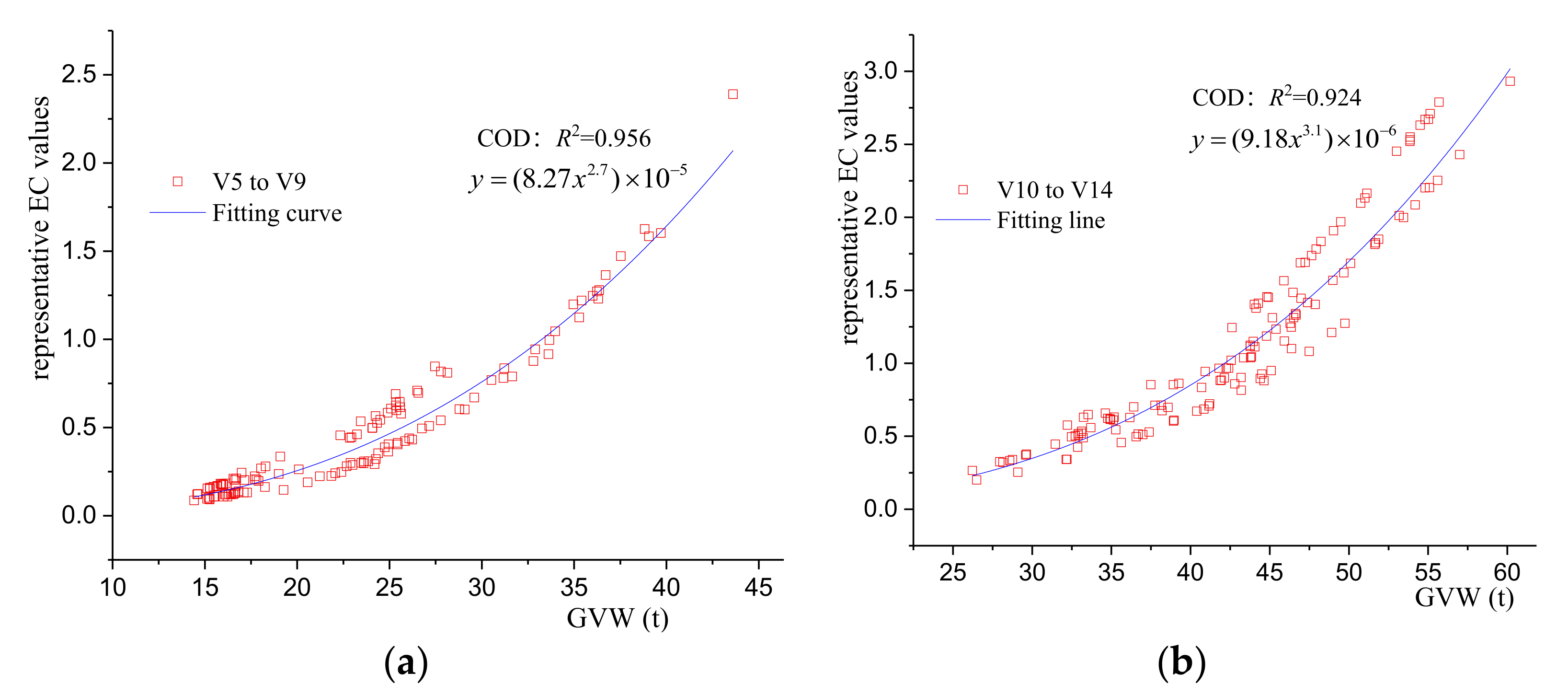
7.1. Calculation for Representative EC Values

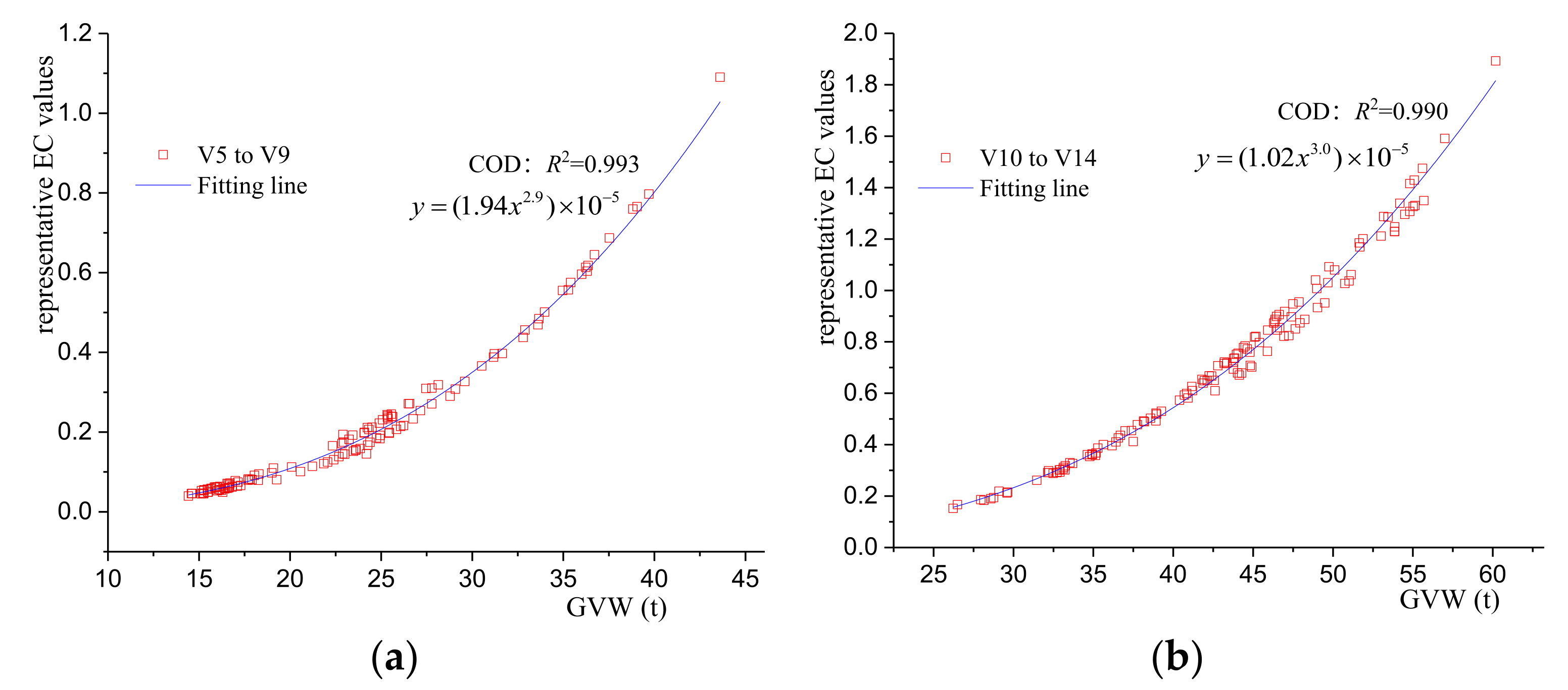
The research shows that there is a significant statistical correlation between the vehicle weight and the representative EC values. Firstly, the representative EC values of each representative vehicle type at 27 locations (No. 9 to 20 in Table 1) are calculated by definition. According to the previous discussion, representative EC values can also be divided into three groups referring to the length of influence line: below 5 m (Group A), 5 to 30 m (Group B), and above 30 m (Group C), as shown in Figure 11, and it can be seen that the correlation between GVW and the representative EC values is very close to a power function, and regression analysis can be used to find the corresponding rules.

Figure 11. Relationship between the GVW and the representative EC values: (a) Group A; (b) Group B; and (c) Group C.

Based on the principle of the least square method, the fitting function of Origin Software (2017 version) is used to fit and analyze the relationship between the gross vehicle weight (GVW) and the representative EC values of each vehicle type in the investigated locations under different influence line lengths. The matching degree between fitting curve and the data is evaluated by the value of the coefficient of determination (COD) $R^2$. The closer that the $R^2$ is to 1, the better the fitting curve that is fitted, and the better the fitting curve can explain the relevant data. Once it exceeds 0.9, it is generally believed that the fitting curve has a strong correlation with the corresponding coefficient.

The results of regression analysis are shown in Figure 12, Figure 13 and Figure 14. The shorter the influence line is, the more divergent the data is, and the more fitting curves are needed for regression analysis. All the fitting curves are power function curves, and the corresponding determination coefficient is above 0.92.

Figure 12. Regression analysis for Group A: (a) V5 to V6; (b) V7 to V8; (c) V9 to V10; and (d) V11 to V14.

Figure 13. Regression analysis for Group B: (a) V5 to V9; (b) V10 to V14.

Figure 14. Regression analysis for Group C: (a) V5 to V9 and (b) V10 to V14.

The formulas corresponding to the fitting curves in Figure 12, Figure 13 and Figure 14 reflects the mathematical relationship between the representative EC values (y) and GVM (x). For convenience, following the conservative principle, the fitting formulas with the same axle number of the vehicle are simplified and merged. As shown in Table 9, the representative EC values can be directly determined according to the number of axles and the GVM of the vehicle.

Table 9. Calculation formula of the representative EC values ($\times {10}^{-5}$).

Number of Axles	Length of Influence Line
	5 m Below	5 to 30 m	30 m Above
2	$y=2.77x^{3.5}$	$y=8.27x^{2.7}$	$y=1.94x^{2.9}$
3	$y=1.38x^{3.5}$
4	$y=2.75x^{2.9}$
5	$y=4.45x^{2.6}$	$y=0.92x^{3.1}$	$y=1.02x^{3.0}$
6 (or more)

7.2. Verification

$Q_{E,fit}$ denotes the equivalent heavy vehicle flow that is calculated based on the fitting formula method that is given in Section 7.1. $Q_E$ denotes the equivalent heavy vehicle flow based on the definition in Section 6.1. $Q_E$ is obtained directly by damage calculation and can be considered to comply with the principle of fatigue damage equivalence. Therefore, $Q_{E,fit}/Q_E$ can be used to verify the validity of the methodology that is given in Section 7.1. As shown in Figure 15. It can be seen that almost all the data fall within the range of 0.85 to 1.15. It indicates that the calculation deviation for the methodology that is given in Section 7.1 is within 15%. Compared with Figure 10, it can be concluded that $Q_{E,fit}$ that is obtained by the proposed method is obviously closer to $Q_E$ than $Q_D$ that is obtained based on the existing standards, and the possibility of underestimating the fatigue load is greatly reduced. The validity and advance are, therefore, proven.

Figure 15. $Q_{E,fit}/Q_E$at different locations.

7.3. Grades for Design Frequency

According to the previous discussion, the calculation of EADTF requires the necessary traffic investigation and is not a simple process. The design service life of the bridge is also an important factor to be considered, which is related to the bridge grade. Therefore, the design load grades are often given in the specifications. In the European code [13], the design frequency of the standard vehicle is divided into four levels, which can be easily selected by designers according to the traffic level. The design load grading is also helpful for designers to understand the load level of the bridge as a whole.

China’s current design code (JTG d64-2015) gives a suggestion for ADTF calculation through the proportion of effective vehicles (above 10 t) in the total traffic flow, which is divided into four levels to choose based on the road function and grade. However, it is no longer suitable for use when the concept of EADTF is adopted. Therefore, the grading suggestions of the design frequency in the slow lane that are based on EADTF are given in Table 10. Through the statistical analysis on EADTF in the slow lane at all the investigated locations (35 in total), the cumulative probability distribution of the change of the slow-lane EADTF can be obtained, as shown in Figure 16. Then, the cumulative frequency of the EADTF corresponding to 50%, 70%, and 90% is taken as the three grades, as shown in Table 9. In the process of fatigue design, after calculating the EADTF that is based on the traffic investigation, the fatigue load level that is close to it can be conservatively selected as the design frequency of the standard vehicle. When the traffic survey data is not available, designers can also choose an appropriate fatigue design load level directly according to the traffic level, but more relative research should be conducted so that much clearer guidelines will be provided for designers.

Table 10. Grades for design frequency (×10⁴ vehicles/year).

Design Frequency of the Standard Vehicle	Cumulative Frequency	Length of Influence Line
		5 m Below	5–30 m	30 m Above
Level 1	50%	100	130	80
Level 2	70%	140	180	110
Level 3	90%	230	265	155

Figure 16. The cumulative distribution of EADTF of the 35 locations.

7.4. Procedure for Determining the Design Frequency

Based on the discussion above, the design frequency of the standard vehicle can be determined by the following steps:

(1)

Necessary traffic investigation, analysis, and prediction;

(2)

Vehicle classification referring to Table 2;

(3)

The corresponding fatigue load spectra of the effective vehicles (with a GVW above 10 t) is obtained;

(4)

The representative EC values are determined referring to Table 9;

(5)

The EADTF can be calculated based on the representative EC values and ADTF

(6)

The corresponding level of design fatigue load is selected and the design frequency of the standard vehicle in the slow lane is finally determined based on the EADTF.

8. Conclusions

When the standard fatigue vehicle load model is adopted in fatigue analysis, the fatigue load will probably be underestimated due to the limitation of the frequency calculation method that is recommended by the existing standard. To solve this problem, in this paper, the fatigue vehicle load data of 35 highway sites involving 15 provinces in China were collected from weigh-in-motion (WIM) systems or existing research, and analysis and discussion were made from the perspective of fatigue damage equivalence. The main conclusions are as follows:

(1)

During the fatigue analysis for steel bridges, it was suggested that the vehicle’s damage contribution with a GVW that is less than 10 t should be ignored;

(2)

In view of fatigue damage equivalence, it was reasonable to utilize EADTF, which is defined as the product of the representative EC values and ADTF, rather than ADTF in the calculation of the design frequency of the standard vehicle in fatigue analysis;

(3)

A practical method was proposed to determine the representative EC values according to the number of axles and the GVW of the vehicle;

(4)

A total of three grades for design frequency of the standard vehicle were put forward based on the statistical analysis of EADTF at 35 locations;

(5)

The steps to determine the design frequency of the standard vehicle in slow lane were given based on the EADTF calculation and the fatigue design load grades.

References

- Doebling, S.W.; Farrar, C.R. The State of the Art in Structural Identification of Constructed Facilities; Los Alamos National Laboratory: Santa Fe, NM, USA, 1999. Available online: https://scholar.google.com/scholar?hl=zh-CN&as_sdt=0%2C5&q=+The+state+of+the+art+in+structural+identification+of+constructed+facilities&btnG= (accessed on 17 December 2021).
- Wolchuk, R. Lessons from weld cracks in orthotropic decks on three European bridges. J. Struct. Eng. 1990, 116, 75–84. [Google Scholar] [CrossRef]
- de Jong, F.B.P. Overview Fatigue Phenomenon in Orthotropic Bridge Decks in the Netherlands; American Society of Civil Engineers (ASCE): Reston, VA, USA, 2004; pp. 1–24. Available online: https://scholar.google.com.hk/scholar?hl=zh-CN&as_sdt=0%2C7&q=Overview+Fatigue+Phenomenon+in+Orthotropic+Bridge+Decks+in+the+Netherlands&btnG= (accessed on 17 December 2021).
- Zhang, Q.H.; Bu, Y.Z.; Li, Q. Review on fatigue problems of orthotropic steel bridge deck. China J. Highw. Transp. 2017, 30, 14–30. [Google Scholar] [CrossRef]
- Dexter, R.J.; Ocel, J.M. Manual for Repair and Retrofit of Fatigue Cracks in Steel Bridges; Federal Highway Administration: Washington, DC, USA, 2013. Available online: https://rosap.ntl.bts.gov/view/dot/38780 (accessed on 17 December 2021).
- Zettlemoyer, N. Stress Concentration and Fatigue of Welded Details; Lehigh University: Bethlehem, PA, USA, 1976; Available online: https://scholar.google.com/scholar?hl=zh-CN&as_sdt=0%2C5&q=Stress+concentration+and+fatigue+of+welded+details&btnG= (accessed on 17 December 2021).
- Byers, W.G.; Marley, M.J.; Mohammadi, J.; Nielsen, R.J.; Sarkani, S. Fatigue reliability reassessment applications: State-of-the-art paper. J. Struct. Eng. 1997, 123, 277–285. [Google Scholar] [CrossRef]
- Wang, G. On Enlightenment & Thinking of Bridge Collapse Accidents Treatment in America & South Korea. China Munic. Eng. 2012, 6, 61–63. [Google Scholar] [CrossRef]
- Ya, S.; Yamada, K. Fatigue Durability Evaluation of Trough to Deck Plate Welded Joint of Orthotropic Steel Deck. Doboku Gakkai Ronbunshuu A 2008, 64, 603–616. Available online: https://www.jstage.jst.go.jp/article/jsceseee/25/2/25_2_33s/_pdf/-char/ja (accessed on 17 December 2021).
- Yoshitake, I.; Hasegawa, H. Moving-wheel fatigue durability of cantilever bridge deck slab strengthened with high-modulus CFRP rods. Structures 2021, 34, 2406–2414. [Google Scholar] [CrossRef]
- Zhu, Z.; Huang, Y.; Xiang, Z. Vehicle load spectrum and fatigue vehicle model of heavy freight Highway. J. Traffic Transp. Eng. 2017, 17, 13–24. [Google Scholar] [CrossRef]
- JTG D64; Specifications for Design of Highway Steel Bridge; China Communication Press: Beijing, China, 2015; Available online: https://scholar.google.com/scholar?hl=zh-CN&as_sdt=0%2C5&q=Specifications+for+design+of+highway+steel+bridge&btnG= (accessed on 17 December 2021).
- EN 1991-2; Actions on Structures-Part 2: Traffic Loads on Bridges; European Committee for Standardization: Brussel, Belgium, 2003; Available online: https://scholar.google.com/scholar?hl=zh-CN&as_sdt=0%2C5&q=Designers%27+Guide+to+EN+1992-2%3A+Eurocode+2%3A+Design+of+Concrete+Structures%3A+Part+2%3A+Concrete+Bridges&btnG= (accessed on 17 December 2021).
- Cohen, H.; Fu, G.; Dekelbab, W.; Moses, F. Predicting truck load spectra under weight limit changes and its application to steel bridge fatigue assessment. J. Bridge Eng. 2003, 8, 312–322. [Google Scholar] [CrossRef]
- Yan, S.; Xiao, R.; Pan, S. Effect on Truck on Freeway after Carrying out GB 1589-2016. China Transp. Rev. 2017, 39, 43–46. Available online: https://scholar.google.com.hk/scholar?hl=zh-CN&as_sdt=0%2C5&q=Effect+on+truck+on+freeway+after+carrying+out+GB+1589-2016&btnG= (accessed on 17 December 2021).
- Žnidarič, A. Heavy-Duty Vehicle Weight Restrictions in the EU. Enforcement and Compliance Technologies. In 23th ACEA Scientific Advisory Group Report; European Automobile Manufacturers Association: Brussels, Belgium, 2015; Available online: https://scholar.google.com.hk/scholar?hl=zh-CN&as_sdt=0%2C5&q=Heavy-duty+vehicle+weight+restrictions+in+the+EU&btnG= (accessed on 17 December 2021).
- Deng, L.; Nie, L.; Zhong, W.; Wang, W. Developing Fatigue Vehicle Models for Bridge Fatigue Assessment under Different Traffic Conditions. J. Bridge Eng. 2021, 26, 04020122. [Google Scholar] [CrossRef]
- AASHTO. LRFD Bridge Design Specification, 9th ed.; American Association of State Highway and Transportation Officials: Washington, DC, USA, 2020; Available online: https://trid.trb.org/view/1704698 (accessed on 17 December 2021).
- Zhou, Y.; Bao, W. Study of standard fatigue design load for steel highway bridges. China Civ. Eng. J. 2010, 11, 79–85. [Google Scholar] [CrossRef]
- Liu, Y.; Li, D.; Zhang, Z.; Zhang, H. Fatigue load model using the weigh-in-motion system for highway bridges in China. J. Bridge Eng. 2017, 22, 04017011. [Google Scholar] [CrossRef]
- Chen, W.; Xu, J.; Yan, B.; Wang, Z.P. Fatigue load model for highway bridges in heavily loaded areas of China. Adv. Steel Constr. 2015, 11, 322–333. [Google Scholar]
- Iatsko, O.; Babu, A.R.; Stallings, J.M.; Nowak, A.S. Weigh-in-Motion-Based Fatigue Damage Assessment. Transp. Res. Rec. 2020, 2674, 710–719. [Google Scholar] [CrossRef]
- Chotickai, P.; Bowman, M.D. Truck models for improved fatigue life predictions of steel bridges. J. Bridge Eng. 2006, 11, 71–80. [Google Scholar] [CrossRef]
- Lehner, P.; Krejsa, M.; Pařenica, P.; Křivý, V.; Brožovský, J. Fatigue damage analysis of a riveted steel overhead crane support truss. Int. J. Fatigue 2019, 128, 105190. [Google Scholar] [CrossRef]
- Zhang, Q.; Fu, L.; Xu, L. An efficient approach for numerical simulation of concrete-filled round-ended steel tubes. J. Constr. Steel Res. 2020, 170, 106086. [Google Scholar] [CrossRef]
- Fisher, J.W.; Roy, S. Fatigue damage in steel bridges and extending their life. Adv. Steel Constr. 2015, 11, 250–268. [Google Scholar] [CrossRef]
- Fatemi, A.; Yang, L. Cumulative fatigue damage and life prediction theories: A survey of the state of the art for homogeneous materials. Int. J. Fatigue 1998, 20, 9–34. [Google Scholar] [CrossRef]
- Liang, Y.; Xiong, F. Study of a fatigue load model for highway bridges in Southeast China. Građevinar 2020, 72, 21–32. [Google Scholar] [CrossRef]
- Lu, N.; Noori, M.; Liu, Y. Fatigue reliability assessment of welded steel bridge decks under stochastic truck loads via machine learning. J. Bridge Eng. 2017, 22, 04016105. [Google Scholar] [CrossRef]
- Wassef, W.G.; Kulicki, J.M.; Nassif, H.; Mertz, D.; Nowak, A.S. Calibration of AASHTO LRFD Concrete Bridge Design Specifications for Serviceability. In NCHRP Report 12-78; Transportation Research Board: Washington, DC, USA, 2014; Available online: https://scholar.google.com.hk/scholar?hl=zh-CN&as_sdt=0%2C5&q=Calibration+of+AASHTO+LRFD+Concrete+Bridge+Design+Specifications+for+Serviceability&btnG= (accessed on 17 December 2021).
- Wang, T. Investigation Statistics and Simulation for Random Traffic Loading of Expressway Bridge; Chang’an University: Chang’an, China, 2010; Available online: https://scholar.google.com.hk/scholar?hl=zh-CN&as_sdt=0%2C5&q=%E9%AB%98%E9%80%9F%E5%85%AC%E8%B7%AF%E6%A1%A5%E6%A2%81%E4%BA%A4%E9%80%9A%E8%8D%B7%E8%BD%BD%E8%B0%83%E6%9F%A5%E5%88%86%E6%9E%90%E5%8F%8A%E4%BB%BF%E7%9C%9F%E6%A8%A1%E6%8B%9F&btnG= (accessed on 17 December 2021).
- Zhuang, M.; Miao, C.; Chen, R. Analysis for Stress Characteristics and Structural Parameters Optimization in Orthotropic Steel Box Girders based on Fatigue Performance. KSCE J. Civ. Eng. 2019, 23, 2598–2607. [Google Scholar] [CrossRef]
- Getachew, A. Traffic Load Effects on Bridges, Statistical Analysis of Collected and Monte Carlo Simulated Vehicle Data; Kungliga Tekniska Hogskolan: Stockholm, Sweden, 2003; Available online: https://scholar.google.com.hk/scholar?hl=zh-CN&as_sdt=0%2C5&q=Traffic+load+effects+on+bridges%2C+statistical+analysis+of+collected+and+Monte+Carlo+simulated+vehicle+data&btnG= (accessed on 17 December 2021).
- Pan, P.; Li, Q.; Zhou, Y.; Li, Y.; Wang, Y. Vehicle Survey and Local Fatigue Analysis of a Highway Bridge. China Civ. Eng. J. 2011, 44, 94–100. Available online: https://scholar.google.com/scholar?hl=zh-CN&as_sdt=0%2C5&q=Vehicle+survey+and+local+fatigue+analysis+of+a+highway+bridge&btnG= (accessed on 17 December 2021).
- Chen, B. Research on Fatigue Load Model and Fatigue Performance Evaluation Method of Steel Bridge Based on WIM Data; Zhejiang University: Hangzhou, China, 2018; Available online: https://scholar.google.com.hk/scholar?hl=zh-CN&as_sdt=0%2C5&q=%E5%9F%BA%E4%BA%8EWIM%E7%9A%84%E7%96%B2%E5%8A%B3%E8%8D%B7%E8%BD%BD%E6%A8%A1%E5%9E%8B%E5%92%8C%E9%92%A2%E6%A1%A5%E7%96%B2%E5%8A%B3%E6%80%A7%E8%83%BD%E8%AF%84%E4%BC%B0%E6%96%B9%E6%B3%95%E7%A0%94%E7%A9%B6&btnG= (accessed on 17 December 2021).
- Xia, Y.; Li, F.; Gu, Y.; Yuan, W.; Zong, Z. Research on vehicle fatigue load spectrum of Highway Bridge Based on WIM. J. Highw. Transp. Res. Dev. 2014, 31, 56–64. [Google Scholar] [CrossRef]
- Shao, Y.; Lu, P. Fatigue Load Spectrum for Jiujiang Yangtze River Bridge. J. Chang’an Univ. (Nat. Sci. Ed.) 2015, 35, 50–56. Available online: https://scholar.google.com.hk/scholar?hl=zh-CN&as_sdt=0%2C5&q=Fatigue+load+spectrum+for+Jiujiang+Yangtze+River+Bridge&btnG= (accessed on 17 December 2021).
- Wang, C. Fatigue Load Spectrum and Fatigue Behaviors of Short Span PC Girder Bridges in Heavy Highway; Beijing Jiaotong University: Beijing, China, 2015; Available online: https://scholar.google.com/scholar?hl=zh-CN&as_sdt=0%2C5&q=%E9%87%8D%E8%BD%BD%E5%85%AC%E8%B7%AF%E5%B0%8F%E8%B7%A8%E5%BE%84PC%E6%A2%81%E6%A1%A5%E7%96%B2%E5%8A%B3%E8%BD%A6%E8%BE%86%E8%8D%B7%E8%BD%BD%E8%B0%B1%E4%B8%8E%E7%96%B2%E5%8A%B3%E6%80%A7%E8%83%BD%E7%A0%94%E7%A9%B6&btnG= (accessed on 17 December 2021).
- Di, J.; Wang, J.; Peng, Q.; Qin, F.; Dai, J. Research and Application of Fatigue Load Spectrum of Port Highway Bridge. J. Chang’an Univ. (Nat. Sci. Ed.) 2018, 38, 48–55. Available online: https://scholar.google.com/scholar?hl=zh-CN&as_sdt=0%2C5&q=%E6%B8%AF%E5%8F%A3%E5%85%AC%E8%B7%AF%E6%A1%A5%E6%A2%81%E7%96%B2%E5%8A%B3%E8%8D%B7%E8%BD%BD%E8%B0%B1%E7%A0%94%E7%A9%B6%E4%B8%8E%E5%BA%94%E7%94%A8&btnG= (accessed on 17 December 2021).
- Hu, S. Study on fatigue load spectrum of expressway bridges in Guangxi. Highw. Eng. 2019, 44, 209–215. [Google Scholar] [CrossRef]
- Li, X.X.; Ren, W.X.; Zhong, J.W. Standard fatigue truck on montane speedway bridge. J. Vib. Shock. 2012, 31, 96–100. [Google Scholar] [CrossRef]
- Amzallag, C.; Gerey, J.P.; Robert, J.L.; Bahuaud, J. Standardization of the rain flow counting method for fatigue analysis. Int. J. Fatigue 1994, 16, 287–293. [Google Scholar] [CrossRef]
Publisher’s Note: MDPI stays neutral with regard to jurisdictional claims in published maps and institutional affiliations. |
© 2022 by the authors. Licensee MDPI, Basel, Switzerland. This article is an open access article distributed under the terms and conditions of the Creative Commons Attribution (CC BY) license (https://creativecommons.org/licenses/by/4.0/).