Numerical Solutions for Chloride Diffusion Fluctuation in RC Elements from Corrosion Probability Assessments

Abstract

Mechanical diffusion of chloride ions in reinforced concrete (RC) structures varies in time and space, and depends on uncertain factors such as material properties, temperature, humidity, and aging. In this paper, different scenarios considering the time of corrosion initiation and the influence of the chloride diffusion coefficient for different loadings (i.e., constant, sinusoidal, Gaussian, and random) were proposed. Stochastic analyses were carried out to estimate the probability of failure of steel bars, and to evaluate the influences of the internal and external factors. Advanced numerical solutions were developed to account for these influences under non-constant diffusion coefficient and non-steady-state condition. Results show that the chloride content can assume low values by using the oscillations of the generic function (e.g., sinusoidal and general) instead of constant function. The influence of the temperature appears relevant. The 3D analyses, considering the random variability, show that chloride content can be higher than ~1.50 compared to chloride content using traditional approaches. Stochastic approaches plus advanced solutions allow, in a more complete way, the sustainability decision-making process during the design phase, maintenance, inspections, and repair.

1. Introduction

Reinforced concrete (RC) is widely used in structures, which are subjected to mechanical and environmental actions (e.g., hot/cold temperature, high/low humidity, strong/weak rainfall) affecting their performance [1,2]. The chloride attack is the most important phenomenon—between the environmental sources of degradation—which is responsible for starting the electrochemical corrosion of reinforcement steel bars [3,4].

The amount of chloride ions in concrete element surfaces depends on its exposure to the surrounding environment as treated in [5]. The chloride penetration, towards the embedded steel reinforcement bars, varies over time and it predominates in a marine atmosphere environment as shown in [1]. Instead, in industrial areas the carbonation-initiated reinforcement corrosion prevails since the environmental pollution reaches a significant carbon dioxide concentration [6].

The corrosion leads to the reduction of the cross-section area of steel reinforcements, concrete-steel strengths (associated to the modifications on the steel internal microstructure), and cracking of concrete cover. Moreover, corrosion products are also expansive, and they can further degrade the concrete [7,8].

In the literature, there are some studies that treat these phenomena as the diffusivity coefficient considering the damage and cracks in reinforced concrete [9,10]; the reduction of the cross-section, which can be deduced in terms of the mass and ductility [11]; the complete model of chloride ingress considering the realistic climate [12], where many factors such as chloride binding, temperature, and humidity were considered.

Other studies treat the chloride diffusion by separating a convection zone with a diffusion zone, where the maximum surface chloride concentration happens at a certain depth inside the structure [13,14,15] or by considering the external loads such as the bending loads [16]. Additionally, interesting case studies, in which how the steel reinforcement corrosion affects the strength and stiffness of the concrete, as well as the behavior of the structure in terms of frequencies were studied in [17].

Alternative approaches are, for instance, the chloride penetration in RC structures by electrical voltage to describe the diffusion flux of different ionic species [18], the chloride content for several layers of concrete [19], and the chloride content effects in RC elements with respect to the structure/sea distance [6,20].

Additionally, some papers study the diffusivity in a probabilistic way [21,22,23], in particular, in [24] the chloride profile is analyzed assuming an irregular trend. The 2D model can be used to better quantify the chloride concentration as shown in [25,26]; however, most of the studies have been carried out using a 2D deterministic model. In ref. [27], from several collected data some distributions have been obtained to provide universal mean values for diffusivity, surface chloride, and threshold chloride. In ref. [28], the durability of a RC element has been studied using the probability of failure induced by concrete cracks under service loads.

In ref. [29], the chloride-induced corrosion in RC structures was treated by probabilistic methods as the first order reliability method (FORM) and the Monte Carlo simulation (MCS) (also studied in this paper), highlighting their benefits in predicting the service life.

In ref. [30], a probabilistic analysis to estimate the probability of corrosion has been carried out, showing the importance of the age, compressive strength, and cover of the concrete. It has been observed that structures older than 50 years with high concrete cover accumulate non-acceptable chloride content affecting their service life. Additionally, in [30], an interesting state-of-the-art regarding the chloride studies was listed.

The main goals of this paper are to estimate: (i) the corrosion initiation time of the steel bars with the chloride ions diffusion and (ii) the influence of the chloride diffusion coefficient under different types of loading. For the former, probabilistic analyses were used to determine the best scenario; thus, for the latter, fluctuation chloride contents were calculated by advanced numerical solutions.

Analyzing the chloride diffusion coefficient by probabilistic analyses plus advanced solutions should model the chloride diffusion in an RC element well. Additionally, as mentioned in [29], the probabilistic models “can be used to help designers quantify how changes to the structural design and maintenance will affect its probability of corrosion and service life”. For this, probabilistic approaches are also used for other applications [31,32].

In this sense, this paper is consistent with goal 9 of the 2030 Agenda [33] in order to “build resilient infrastructure, promote inclusive and sustainable industrialization and foster innovation” but also to “develop quality, reliable, sustainable and resilient infrastructure, including regional and transborder infrastructure, to support economic development and human well-being, with a focus on affordable and equitable access for all”.

2. Mechanical Model

2.1. Problem Statement

The flux of chloride ions J (expressed in kg/(m² s)) in saturated concrete depends on the chloride concentration gradient ∇C (C is expressed in kg/m³) as described by Fick’s first law [34]:

$$\mathrm{J}=-{\mathrm{D}}_{\mathrm{cl}}\nabla \mathrm{C}$$

(1)

where D_cl is the diffusivity (or diffusion coefficient, expressed in cm²/year) that can be variable or constant (i.e., independent of the position and time).

D_cl can also be called “apparent” diffusivity when regarding the volume of the concrete element [35] and when it takes into account the effect of cracks on the diffusion [29]; or “effective” diffusivity when it is taken as a random variable having its characteristics based on a time-invariant mean value fitting the diffusion model well [29].

By deriving Equation (1) through the mass balance principle over time t (i.e., non-steady state) in the direction i, the partial differential equation (PDE), called Fick’s kinetic second law, is obtained as:

$$\frac{\partial \mathrm{C}}{\partial \mathrm{t}}=\nabla \left({\mathrm{D}}_{\mathrm{cl},\mathrm{i}}\nabla {\mathrm{C}}_{\mathrm{i}}\right)=\frac{\partial }{\partial \mathrm{i}}\left({\mathrm{D}}_{\mathrm{cl}}\frac{\partial \mathrm{C}}{\partial \mathrm{i}}\right)$$

(2)

The full chloride concentration is divided in dissolved free concentration C_f and chemically binding concentration C_b due to the reaction of the cement hydration products. They can be correlated between them as [36,37]:

$$\mathrm{C}={\mathsf{\omega }}_{\mathrm{e}}{\mathrm{C}}_{\mathrm{f}}+{\mathrm{C}}_{\mathrm{b}}$$

(3)

where ω_e is the evaporable water content. ω_e plus the non-evaporable water content, ω_n, provide the full water content ω as ω = ω_e + ω_n [38].

C_b concentrations depend on, e.g., the type and composition of cement, temperature, and they include the interaction/reaction or absorption with the solid cement [39].

The correlations between C_f and C_b at a given temperature are known as Langmuir isotherms, that, with two parameters correlated to the concrete properties (i.e., α = 11.80, β = 4.0), can be defined by [37,40,41]:

$${\mathrm{C}}_{\mathrm{b}}=\frac{{\mathsf{\alpha } \mathrm{C}}_{\mathrm{f}}}{1+{\mathsf{\beta }\mathrm{C}}_{\mathrm{f}}}$$

(4)

Consistent with Equation (3), if the chloride binding effects are considered (i.e., C_b ≠ 0), the chloride concentration corresponds to the total chloride content (i.e., free + binding), whereas if they are neglected (i.e., C_b = 0), the chloride concentration is equal to the C_f concentration since, as mentioned in [29], “the process of the binding continues to remove chlorides from the pore solution”. The diffusion–binding interactions provide an anomalous chloride diffusion that does not strictly obey Equation (2).

2.2. Analytical Solution

From Equation (2), the differential relation in the x direction, with Dirichlet’s boundary (b.c.) and initial (i.c.) conditions [36,38], is:

$$\frac{\partial \mathrm{C}}{\partial \mathrm{t}}={\mathrm{D}}_{\mathrm{cl}}\frac{{\partial }^2\mathrm{C}}{\partial {\mathrm{x}}^2}$$

(5)

$$\begin{array}{cc}\mathrm{i}.\mathrm{c}.:& \mathrm{C}\left(\mathrm{x},0\right)={\mathrm{C}}_0\\ \mathrm{b}.\mathrm{c}.:& \mathrm{C}\left(0,\mathrm{t}\right)={\mathrm{C}}_{\mathrm{s}}\\ & \mathrm{C}\left(\infty ,\mathrm{t}\right)={\mathrm{C}}_0\end{array}$$

where C₀ is the inner chloride concentration and C_s is the chloride concentration at the external concrete surface. C_s is applied at the external face; thus, it can be considered as the “loading” parameter as mentioned in [29]; whereas C₀ is applied at the opposite face.

Equation (5) can be solved under some hypotheses. Some of these are stronger than others considering the mathematical conditions, i.e., (1) the medium is considered semi-infinite (i.e., at x = ∞, C₀ assumes a defined constant value); (2) C_s is uniform in space and constant in time; (3) D_cl is constant in space and time; and (4) the diffusion is mono-dimensional.

These four hypotheses are mandatory to obtain the analytical solution (Equation (6)).

Other hypotheses regard physical concepts, i.e., (5) concrete is saturated (e.g., permanently submerged in seawater) and homogeneous; (6) the external surface of the concrete is a plane; and (7) the chloride ions are diffused into a water-saturated concrete without interacting with the other species.

The hypothesis 7 should be valid since the diffusion coefficient represents a very slow rate (~10⁻¹²−10⁻¹¹ m²/s [29]); therefore, the chloride ions remain almost in equilibrium during the diffusion process. This slow speed is because chloride diffusion occurs in pores that are filled with water and not in pores filled with air.

In ref. [21], these hypotheses were discussed in detail showing the motivations in adopting them and the possible alternatives.

Therefore, under these hypotheses, the analytical solution of Equation (5) is:

$$\mathrm{C}={\mathrm{C}}_0+\left({\mathrm{C}}_{\mathrm{s}}-{\mathrm{C}}_0\right)\left(1-\mathrm{erf}\frac{\mathrm{x}}{2\sqrt{{\mathrm{D}}_{\mathrm{cl}} \mathrm{t}}}\right)$$

(6)

where the erf(·) is the Gaussian error function integrated between 0 and x/[2$\sqrt{{\mathrm{D}}_{\mathrm{cl}} \mathrm{t}}$].

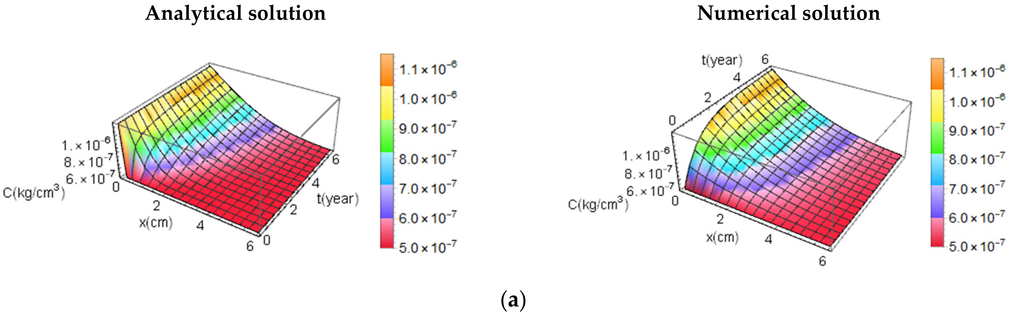
2.3. Numerical Solution

The numerical analysis was considered by solving the system of PDEs. They allow to obtain other results reducing some abovementioned hypotheses, i.e., they can be developed in 2D and 3D (spatial variability), and accounting for the time variability.

The differential equation in the x-direction, with i.c. and b.c., is [36,38]:

$$\frac{\partial \mathrm{C}}{\partial \mathrm{t}}={\mathrm{D}}_{\mathrm{cl}}\frac{{\partial }^2\mathrm{C}}{\partial {\mathrm{x}}^2}$$

(7)

$$\begin{array}{cc}\mathrm{i}.\mathrm{c}.:& \mathrm{C}\left(\mathrm{x},0\right)={\mathrm{C}}_0\\ \mathrm{b}.\mathrm{c}.:& \mathrm{C}\left(0,{\mathrm{t}}_{\mathrm{m}}\right)={\mathrm{C}}_{\mathrm{s}}\\ & \mathrm{C}\left({\mathrm{x}}_{\mathrm{m}},{\mathrm{t}}_{\mathrm{m}}\right)={\mathrm{C}}_0\end{array}$$

where x_m is the position variable and t_m is the time variable (detailed in Section 5.2).

To develop the numerical analyses by differential equations, the i.c. and b.c. (Equation (7)) must be a priori determined to avoid the generation of the arbitrary constants associated with i.c. and b.c. Therefore, it is necessary to quantify both conditions to find the solutions [42].

Additionally, a convergence process is necessary to define the “stop” of the analyses.

The convergence procedure consists of the (i) definition of the f_D(i,t) function that should describe a loading; (ii) definition of the b.c. in the numerical analysis; and (iii) plotting of the 2D/3D chloride content curves C(i,t). The verification of this procedure between the exact, E_s, and numerical solutions, N_s, is caried out by [21]:

$$\left|\mathrm{C}{\left(\mathrm{i},\mathrm{t}\right)}_{{\mathrm{E}}_{\mathrm{s}}}^{{\mathrm{k}}_{\mathrm{s}}}-\mathrm{C}{\left(\mathrm{i},\mathrm{t}\right)}_{{\mathrm{N}}_{\mathrm{s}}}^{{\mathrm{k}}_{\mathrm{s}}}\right|\le \mathsf{\epsilon }$$

(8)

where ε denotes a specific convergence parameter (here ε = 1.50 × 10⁻⁹ [21,23]) and k_s represents the iterations. Therefore, this convergence is completed reducing the analytical/numerical result differences.

In the 3D model, with the variables t and i = x, y, the convergence between an exact/numerical solution could be evaluated through the sum of square errors (SSE) as [21]:

$$\mathrm{SSE}={\displaystyle \sum }_{\mathrm{k}=1}^{\mathrm{n}}\left[{\left(\mathrm{C}{\left(\mathrm{i}\right)}_{{\mathrm{E}}_{\mathrm{s}}}^{{\mathrm{k}}_{\mathrm{s}}}-\mathrm{C}{\left(\mathrm{i}\right)}_{{\mathrm{N}}_{\mathrm{s}}}^{{\mathrm{k}}_{\mathrm{s}}}\right)}^2+\mathrm{w}{\left(\mathrm{C}{\left(\mathrm{t}\right)}_{{\mathrm{E}}_{\mathrm{s}}}^{{\mathrm{k}}_{\mathrm{s}}}-\mathrm{C}{\left(\mathrm{t}\right)}_{{\mathrm{N}}_{\mathrm{s}}}^{{\mathrm{k}}_{\mathrm{s}}}\right)}^2\right]$$

(9)

where w is a weight factor indicating the relative error (here w = 1.0). Therefore, the convergence finishes when SSE|_ks+1 < SSE|_ks stabilizes.

2.4. Chloride Diffusion Coefficient

In this paper, the chloride diffusion coefficient is not considered as a constant coefficient, but it is considered with the following multi-factorial diffusivity [3]:

$${\mathrm{D}}_{\mathrm{cl}}={\mathrm{D}}_{\mathrm{cl},\mathrm{ref}}\times {\mathrm{f}}_1\left(\mathrm{T}\right)\times {\mathrm{f}}_2\left(\mathrm{t}\right)\times {\mathrm{f}}_3\left(\mathrm{h}\right)$$

(10)

where the factors f₁, f₂, and f₃ account for the temperature T, concrete age t, and humidity h, respectively.

The D_cl,ref is called “reference diffusion” since it is based on a certain t, T, and h for fully saturated concrete [7,43]. This factor is usually calculated using equations depending on the water/cement (w/c) ratio, but the authors believe that this unique dependency is very simple; therefore, D_cl,ref was taken a priori from previous studies (i.e., D_cl,ref = 0.40 cm²/year [29,44]).

It is important to highlight that there are several relations used to estimate D_cl as shown in [2,45]. A more complete relation defined in [5,23] is formed by 6 factors, of which 4 factors are shown in Equation (10). In this sense, it is reasonable to affirm that Equation (10) estimates D_cl well.

The factors f₁, f₂, and f₃ are, respectively:

$${\mathrm{f}}_1\left(\mathrm{T}\right)={\mathrm{e}}^{\left[\frac{{\mathrm{E}}_{\mathrm{a}}}{\mathrm{R}}\left(\frac{1}{{\mathrm{T}}_0}-\frac{1}{\mathrm{T}}\right)\right]}$$

(11)

$${\mathrm{f}}_2\left(\mathrm{t}\right)=\left\{\begin{array}{c}\frac{1}{1-\mathrm{m}}{\left(\frac{{\mathrm{t}}_{\mathrm{ref}}}{\mathrm{t}}\right)}^{\mathrm{m}} \mathrm{for} \mathrm{t}<{\mathrm{t}}_{\mathrm{r}}\\ \left[1+\frac{{\mathrm{t}}_{\mathrm{r}}}{\mathrm{t}}\left(\frac{\mathrm{m}}{1-\mathrm{m}}\right)\right]{\left(\frac{{\mathrm{t}}_{\mathrm{ref}}}{\mathrm{t}}\right)}^{\mathrm{m}} \mathrm{for} \mathrm{t}\ge {\mathrm{t}}_{\mathrm{t}}\end{array}\right.$$

(12)

$${\mathrm{f}}_3\left(\mathrm{h}\right)=\frac{1}{\left[1+\frac{{\left(1-\mathrm{h}\right)}^{\mathrm{n}}}{{\left(1-{\mathrm{h}}_{{\mathrm{D}}_{\mathrm{cl}}}\right)}^{\mathrm{n}}}\right]}$$

(13)

The factor f₁ (expressed in K) is given by Arrhenius’ law [37,40,43,46], where T₀ is the reference temperature (T₀ = 296.0 K, i.e., 23.0 °C); E_a is the activation energy of the diffusion process correlated to the w/c ratio; and R is the universal ideal gas constant, which is correlated to the molar concentration, chemical potential of the present species, and T (R = 8.314 J/(mol K)) [47].

The factor f₂ affects the diffusivity due to the continuous hydration [16,37,43], where t_ref is the reference concrete age (t_ref = 28 days, i.e., 0.076 years); t_r is the time when the diffusivity is assumed to be constant (t_r = 30.0 years); and t is considered as the “exposed time” (t = 25.0 years). The parameter m reduces the speed of chloride diffusivity and depends on w/c ratio, fly ash, and slag in concrete [48].

Finally, f₃ is calculated by [3,46,49], where h_Dcl is a calibrated humidity with respect to D_cl by several laboratory tests and is assumed at 21.0–25.0 °C, equal to 0.75 [50]. The n-parameter characterizes the spread of the drop in D_cl (n = 4.0 [3,46,48] or 6.0 ≤ n ≤ 16.0 [50]). D_cl strongly depends on h, e.g., for n = 4.0, T = 50.0 °C, h_Dcl = 0.75, and h = 0 the humidity factor is f₃(h) = 3.89 × 10⁻³ [50].

These parameters are shown in

Table 1. Deterministic data.

α [44]	β [44]	Dcl,ref [29]	w/c *	T0 [40]
11.80	4.0	0.40 cm2/year	0.50 a	23.0 °C (296.0 K)
R [40]	tref [43]	T *	tr [43]	hDcl [50]
8.134 J/mol K	28 days (0.076 years)	25.0 years	30.0 years	0.75

Note: * = Adopted value in this study. ^a In ref. [33], from 97 surveyed structures it was suggested to use a value of w/c > 0.40 to avoid an high C_th.

and

Table 2. Random variable data.

Parameter	PDF Distribution	μ	±σ a	CV (%)
Ea (kJ/mol)	Normal	44.60 [40] b	4.30	10.0
T (°C)	Normal	23.0 *c	8.0	35.0
Cf (kg/m3)	Log-normal	1.50 [44]	0.75	50.0
ωe	Beta (5, 1)	0.83 *	0.1408	17.0
m	Beta (1, 4)	0.20 [48]	0.1632	82.0
h	Beta (4, 1)	0.80 *	0.1632	20.0
n	Uniform (0, 12)	6.0 [50]	3.4641	58.0
xc (cm)	Log-normal	5.0 *d	1.50	30.0
C0 (kg/m3)	Uniform (0, 1)	0.50 *	0.2886	58.0
Cs (kg/m3)	Log-normal	1.15 [7] e	0.575	50.0

Note: * Adopted value in this study. CV = coefficient of variation, calculated as (σ/μ) × 100. ^a In the Beta and Uniform PDF, ±σ is calculated by their distribution equations. ^b For w/c = 0.50 and with fluid-free pores [51]. ^c It corresponds to 296.0±8.0 K. ^d It can be considered a fair cover [8]. ^e For structures located between 0.10 and 2.84 km from the coast without direct contact with seawater [7]. This value can reach a value of 7.35 kg/m³ [5] up to 25.0 kg/m³ as indicated in [29].

.

3. Probabilistic Approaches

This probabilistic approach is based on the use of probability density functions (PDFs) and potentially failure modes defined by a limit state (LS) function G(X) [52]. When G(X) < 0 the probability of failure occurs (failure domain), whereas when G(X) > 0 the probability of non-failure occurs (safety domain). Both domains are separated by G(X) = 0 (limit domain).

For N_X samples of each random variable vector X = {x₁, x₂, …, x_j} = {x_i}, and a LS function G(X), the probability of failure is:

$${\mathrm{p}}_{\mathrm{f}}=\mathrm{P}\left[\mathrm{G}\left(\mathrm{X}\right)<0\right]=\underset{\left\{\mathrm{X}: \mathrm{G}\left(\mathrm{X}\right)<0\right\}}{\overset{}{{\displaystyle \int }}}{\mathrm{f}}_{\mathrm{X}}\left({\mathrm{x}}_1,{\mathrm{x}}_2,\dots ,{\mathrm{x}}_{\mathrm{j}}\right){\mathrm{dx}}_1{\mathrm{dx}}_2\dots {\mathrm{dx}}_{\mathrm{j}}=\underset{\left\{\mathrm{X}: \mathrm{G}\left(\mathrm{X}\right)<0\right\}}{\overset{}{{\displaystyle \int }}}{\mathrm{f}}_{\mathrm{X}}\left({\mathrm{x}}_{\mathrm{i}}\right){\mathrm{dx}}_{\mathrm{i}}$$

(14)

where f_X(x_i) are the joint PDFs of the random variables x_i.

Equation (14) is the cumulative failure probability (CFP) calculated as the area of the PDF within a specific interval. This area defines the probability that G(X) takes on a value less than 0.

CFP is the equivalent to the cumulative distribution function (CDF), which is estimated by integrating Equation (14) in the time of failure [20], i.e., CFP ≡ CDF.

The failure in this study can occur at any time and position of concrete (i.e., on the surface or in the middle of concrete cover, as well as in the steel–concrete interface [53]).

In this paper, three methods were implemented: the (i) semi-analytic first order reliability method (FORM), (ii) analytical method called “direct integration (DI)”, and (iii) Monte Carlo simulation (MCS). Similar to [29], here we also compare the FORM results with MSC results.

FORM derives from the fact that the function G(X) is approximated by the first order Taylor expansion, which is a linearization around the design point. In fact, to estimate the probability of failure it is necessary to find a distance, called the reliability index β, between the origin of the limit domain and the most probable point located at the failure surface G(X) = 0. It does not need a large number of interactions and input data.

Figure 1 shows a general illustration of the FORM method; MSC points are also shown.

DI is based on the Rosenblatt transformation [54] and Gaussian distribution. If G(X) is a linear combination of normally distributed random variables x_i, then G(X) also follows a normal distribution; therefore, its mean and standard deviation can be calculated analytically.

Finally, MCS, which generates pseudo-random values, is performed according to the following formulation [55]:

$${\mathrm{P}}_{\mathrm{f}}=\underset{\left\{\mathrm{X}: \mathrm{G}\left(\mathrm{X}\right)<0\right\}}{\overset{}{{\displaystyle \int }}}\mathrm{I}\left({\mathrm{x}}_{\mathrm{i}}\right){\mathrm{f}}_{\mathrm{X}}\left({\mathrm{x}}_{\mathrm{i}}\right){\mathrm{dx}}_{\mathrm{i}}$$

(15)

$$\mathrm{I}\left({\mathrm{x}}_{\mathrm{i}}\right)=\left\{\begin{array}{c}1, \mathrm{for} \mathrm{G}\left(\mathrm{X}\right)\le 0\\ 0, \mathrm{for} \mathrm{G}\left(\mathrm{X}\right)>0\end{array}\right.$$

(16)

$${\mathrm{p}}_{\mathrm{f}}=\frac{1}{\mathrm{N}}{\displaystyle \sum }_{\mathrm{i}=1}^{\mathrm{N}}\mathrm{I}\left({\mathrm{x}}_{\mathrm{i}}\right)=\frac{{\mathrm{N}}_{\mathrm{f}}}{\mathrm{N}}$$

(17)

where I(∙) is an indicator function, N is the number of simulations, and N_f is the number of simulations with I(x_i) ≤ 0. In other words, p_f in Equation (17) can be considered as the mean value of I(x_i), i.e., Ī(x_i) = E[I(x_i)].

The results of p_f are accurate when N → ∞; however, in practice, the number of samples required is 1.0 × 10^k where the choice of k depends on the compute capacity, thus affecting the computation time. In this analysis k = 2 and k = 6 were adopted to quantify the goodness of the analyses.

Here, the LS function is defined considering the time for corrosion initiation t_R and the design structural lifetime t_a. In particular, LS is G(X) = t_R(X) − t_a.

To determine the time t_R(X) in function of the cover depth x_c, Equation (6) was rewritten as [4,7,29]:

$${\mathrm{t}}_{\mathrm{R}}\left(\mathrm{X}\right)=\frac{{\mathrm{x}}_{\mathrm{c}}^2}{4{\mathrm{D}}_{\mathrm{cl}}{\left({\mathrm{erf}}^{-1}\left[\frac{\mathrm{C} -{ \mathrm{C}}_{\mathrm{s}}}{{\mathrm{C}}_0-{ \mathrm{C}}_{\mathrm{s}}}\right]\right)}^2}\approx \frac{{\mathrm{x}}_{\mathrm{c}}^2}{4{\mathrm{D}}_{\mathrm{cl}}{\left(\mathrm{erf}\left[\frac{{\mathrm{C}}_{\mathrm{th}}-{\mathrm{C}}_{\mathrm{s}}}{{\mathrm{C}}_0-{\mathrm{C}}_{\mathrm{s}}}\right]\right)}^2}$$

(18)

where C_th is the chloride threshold concentration. It should not be formed at the steel bar surface to avoid the corrosion of the steel passive layers, in fact the corrosion begins when the chloride concentration reaches the C_th at x_c (i.e., C_th = C(x_c, t_R)). Additionally, when t_R = t_a (i.e., G(X) → 0) the failure occurs.

Strictly speaking, in this study LS divides the “corroded” with the “non-corroded” domain instead of “failure” and “non-failure” domains, respectively; however, both nomenclatures are usually accepted.

The numerical values of the erf (∙) inverse, erf⁻¹(∙), were provided for −1 < input < 1 real range, whereas erf (∙) function ranges between—∞ < input < + ∞; but the real values less than 1 were given only between—3.5 < input < +3.5. Here, the input values have a large range, therefore, erf(∙) was used instead of its inverse.

To quantify the corrosion initiation, Equation (18) does not consider the steel bar diameter [11], the chemical/biological processes and their reactions at the concrete/bars interface [53]. However, Equation (18) provides a useful life advantage since the time related to mechanical processes is expressed in months, whereas for chemical/biological processes it is expressed in years (or centuries) [56].

4. General Methodology

The procedures used in this paper are the (i) probabilistic analysis for defining the probability of failure considering the corrosion initiation time (Section 3) and (ii) the numerical simulations to estimate the chloride content for different chloride coefficients defined by a certain function (Section 2.3 and Section 5.2.1).

The used methodology to study the chloride concentration inside concrete is mainly divided in two parts (see Figure 2).

In part I the D_cl was defined, whereas in part II the chloride concentration C(i, t) was determined. The two parts are explained in the following steps.

Step 1: Here, the first and second Fick’s laws were defined. Factors D_cl,ref, f₁, f₂, and f₃ to obtain the relation of chloride coefficient D_cl,i were evaluated.

Step 2: The deterministic values, the estimation of probabilistic methods, and their random variables were defined. In this sense, D_cl,i is a semi-probabilistic coefficient since only five probabilistic parameters (i.e., m, E_a, n, T, h) were adopted; the other parameters (i.e., D_cl,ref, h_Dcl, R, T₀, w/c, t, t_ref, t_r) were calculated deterministically. These parameters will be better explained in Section 5.1.

Step 3: Implementation of the analytical solutions. In a 2D analysis (in x and t), the variabilities were assumed non-stationary (i.e., they are variable in t and x). In an n-D analytical analysis, the variabilities can still be assumed non-stationary but only for the variabilities that refer to the studied direction (e.g., x₁ and t) keeping the other variables {x₂, x₃, …, x_n} stationary.

Step 4: Implementation of the 2D and 3D numerical solutions. In this step, the unknown functions y_j and independent variables x_j of differential equations were found. These solutions are represented by functions y_j using “interpolating function” (IF), which provides approximated y_j values in x_initial − x_final for x_j. The process is iterative, starting at a value of x_j and taking a sequence of steps, covering the whole range x_initial − x_final. Suitable i.c. and b.c. conditions for the y_j and their derivatives must be defined. In this way, the values for y_j(x_j) and y_j’(x_j) at certain points x_j were specified. More details are available in the authors’ previous studies [21,23].

Step 5: Estimation of the chloride content C(i, t). If the convergence is not found, the i.c. and b.c must be re-defined.

5. Analyses and Results

5.1. Probabilistic Results

The probabilistic analysis considers the parameters as independent random variables in space i and t. Stochastic analyses applied only for the 2D models could not describe the response of RC structures well and thus they could underestimate the failure probabilities [57].

Table 1 and Table 2 list the group of the deterministic and random variables with their multivariate distributions, respectively.

In the Beta distribution B(α’, β’) for the shape parameter α’ = 1, the P(X ≤ x) probability is small, whereas for β’ = 1 it is great. For instance, ω_e is more probable as ω_e > 0.60 (ω_e → 1.0), thus the more appropriate Beta distribution should be obtained for α’ >> β’; the m-parameter is more probable as m < 0.50 (m → 0), thus the more appropriate Beta distribution should be obtained for β’ >> α’.

Figure 3 shows the probabilistic distribution function for each random variable. Figure 4 shows three scenarios by using the three methodologies. Scenario I is calculated using the values indicated in Table 1 and Table 2. In scenarios II and III, T and C_f change.

The input data to plot the p_f vs. t_a curves (Figure 5) were obtained using Equation (17) for MCS, whereas for FORM and DI it was necessary to define μ_tR and σ_tR to estimate the reliability index β and thus p_f.

In DI, μ_tR and σ_tR are obtained using Equation (18) using the values in Table 1 and Table 2. In FORM, μ_tR is the same as the DI but σ_tR is obtained for each t_a.

It is possible to see that, for a prevision at long period and with relatively few samples (i.e., k = 2 for MCS), it is more difficult to estimate failure probabilities. In fact, the MCS curve tends to depart from the DI curve (exact curve) providing non-sharpened shapes in the PDF distributions. For the MCS, the mean and the standard deviation are known, whereas for DI and FORM, the standard deviation was chosen low a priori. However, DI is very sensitive to the used data, which are unknown a priori; thus, could under- or over-estimate the results.

In Figure 4, for scenarios II and III, the p_f curve is lesser than the p_f curve of I scenario. This indicates the low influence of the C_f and the high influence of the T variation.

Table 3. Scenarios of the t_R (year).

	Scenario I a Dcl = 0.423 cm2/Year Cb = 3.31 × 10−6 kg/cm3		Scenario II Dcl = 0.256 cm2/Year Cb = 3.31 × 10−6 kg/cm3		Scenario III Dcl = 0.256 cm2/Year Cb = 4.51 × 10−6 kg/cm3
	μtR (Year)	σtR (Year)	μtR (Year)	σtR (Year)	μtR (Year)	σtR (Year)
MCS	21.44 (14.11) b	14.95 (4.68)	35.41 (23.39)	24.96 (8.01)	35.03 (23.31)	24.58 (7.98)
FORM	14.82	4.21	24.36	6.92	24.36	6.36
DI	14.87	5.20	24.41	8.54	24.41	8.54

^a Used to develop the numerical analyses (Section 5.2). ^b The values in the brackets were obtained by using k = 6 [21].

shows the main values and standard deviations of PDFs. It seems that MSC results provide the worse estimation of 6.49–10.45 years by using relatively few samples. However, this indicates that a low approximation should provide results on the conservative side as also shown in [29].

The used C_th ranges between 3.75 and 4.51 × 10⁻⁶ kg/cm³ [21]. In ref. [30], from 97 surveyed structures, it was shown that when the chloride content at x_c depth is more than 0.20% of the concrete weight (i.e., 4.80 × 10⁻⁶ kg/cm³) the probability of corrosion is more than 90.0%.

5.2. Numerical Results

The 2D/3D analyses were carried out with Mathematica software [42]. The principle of the analysis is based on Hermite polynomials (HPs) explained in [58,59].

Here, the chloride concentration in concrete was analyzed by developing, in a numerical way, a function f_D(i,t) multiplied by D_cl, which was obtained in a probabilistic way. Here, the chloride coefficient function f_D(i,t) was introduced to study four types of loads: constant, sinusoidal, Gaussian, and general.

Here, the dimension of the analyses regarding the flux direction plus the time dependency, i.e., 2D analyses provide the chloride concentration C in x- and t-domains, whereas 3D analyses provide C results in x-, y-, and t-domains [60,61].

5.2.1. The 2D Chloride Diffusion

Some external loadings act on a RC structure by random actions, in this sense, here the load f_D(x,t) can be represented by constant, sinusoidal, Gaussian, and general loadings (see

Table 4. Four generic functions f_D(x,t) and their applications (proposed approach).

Type	Dcl × fD(x,t)	Possible Applications
Constant	Dcl × constant	- Temperature/humidity: they can be considered constant for short climate conditions. - Dead loadings, accidental loadings, hydrostatic loadings, uplifts, wind actions, pseudo-static/dynamic accelerations, etc.
Sinusoidal	Dcl × Sin(t)	- Temperature/humidity: it simulates the seasonal weather with two peaks during one cycle of 2π (one year), i.e., positive (summer) and negative (winter) peak. - Waves: sound, light, sloshing, convective, electromagnetic, nuclear, etc.
Gaussian	${\mathrm{D}}_{\mathrm{cl}}\times {\mathrm{e}}^{-{\mathrm{t}}^2}$	- Concentrate forces in the t-domain. - Impulsive actions: impulsive waves, impulsive pressures, blasts, etc.
General	${\mathrm{D}}_{\mathrm{cl}}\times {{\displaystyle \sum }}_{\mathrm{i}}^{\mathrm{n}}\sin \left(\mathrm{it}+\mathsf{\varphi }\right)$ a	- Earthquakes: shear/compressive/vertical waves, seismic amplifications, etc. - Vibration of machines, wind, etc.

^a ϕ = Angular phase between 0 and 2π.

).

Figure 5 shows the analytical (exact) and numerical solutions for constant f_D(x,t) by using data regarding scenario I.

The exact solution of C(x,t) using Equation (6) is plotted for 0 ≤ x ≤ x_final = 6.0 cm and 0 ≤ t ≤ t_final = 2π years, whereas the C(x,t) numerical solution by Equation (7) for 0 ≤ x_m ≤ x_m,final = 6.0 cm and 0 ≤ t_m ≤ t_m,final = 2π years.

As mentioned in Section 2.3, to obtain the numerical solution the pre-definitions of b.c. C(x_m,t_m) = C₀ (see Equation (7)) is necessary, in particular the term x_m. With x_m = 20 x_m,final, an acceptable convergence was obtained as shown in [23,50].

The horizontal line in the analytical solution (Figure 5c) comes from Equation (6), in fact for x = 0 the concentration is C(x,t) = C_s.

Figure 6, Figure 7 and Figure 8 show the numerical solutions for f_D(x,t) sinusoidal, Gaussian, and general, respectively. The used data refer to scenario I. It is possible to note that the trend of C(x,t) is consistent with the respective used load. The horizontal line in Figure 6c is verified when t = 0 since erf(∞) → 1; thus, C(x,t) = C₀ (see Equation (6)).

By comparing Figure 5, Figure 6, Figure 7 and Figure 8, it is possible to note that, due to the oscillations of the generic function (e.g., sinusoidal, and general), the chloride content C can assume lower values with respect to C values for constant diffusivity. This is evident, for instance, at ~3.0 and 5.5 years (Figure 8d).

5.2.2. The 3D Chloride Diffusion

From Equation (7), the 2D chloride concentration model C(x,t) passes to the 3D C(x,y,t) model. Therefore, the number of the b.c. increases. C(x,y,t) is plotted for 0 ≤ x_m ≤ 6, 0 ≤ y_m ≤ 3, t_m = 2π. In the 3D model, the b.c., regarding C(x_m,y_m,t_m) = C₀, is x_m = 20 x_m,final and y_m = 20 y_m,final.

Figure 9 shows the 3D chloride diffusion by numerical solution. The chloride concentrations are the sum of the values obtained by x and y contributions [25].

Table 5. Comparison of both models.

Chloride Content	2D	3D	3D/2D Ratio
CmIn(i,t)	5.0 × 10−7 kg/cm3 (Figure 5a)	7.20 × 10−7 kg/cm3 (Figure 9c)	1.44 a
CIax(i,t) b	1.15 × 10−6 kg/cm3	1.15 × 10−6 kg/cm3	1.0

^a This ratio was estimated as 1.33 (at t = 5.0 years) in [59], and 1.40 in [25]. ^b It corresponds to C_s (Table 2).

shows some important results and the 3D/2D ratio for comparison. In the 3D model C comes from different directions (spread); therefore, the ratio must be ≥1.0. It is possible to note that for both models the superficial concentration, C_max, assumes similar values since they are subjected to the same conditions. On the other hand, the internal diffusion process provides a different final value, C_min, where steel bars are placed.

6. Conclusions

In this paper, the chloride ion diffusion in RC elements was studied. In an alternative to the traditional 2D analytical analyses, here probabilistic approaches were used to estimate some scenarios; thus, using advanced numerical analyses, the 2D/3D chloride concentration was obtained.

(1)

Three different probabilistic techniques (i.e., MCS, FORM, DI) were used to estimate the probability of failure of steel bars by considering the time of corrosion initiation. The probabilistic analyses were carried out using several simulations for each variable. PDF functions were defined, which have a great importance in practical applications since they enable the analyst to know if the probability of failure is acceptable according to the parameters involved (Table 2 and Figure 2). MCS is a technique used to evaluate some functions using several random variables. For each sample, a random variable is assigned as a deterministic value from which several random numbers are generated. The results are treated as a distribution, and they are statistically determined. MCSs directly provide the t-variant failure probability. Results show a strong influence of the T variation. It was also noted that MCS provides high values in favor of safety, i.e., ~6.5 years (Figure 4 and Table 3) with relatively few samples. A very good agreement was achieved with DI and FORM.

(2)

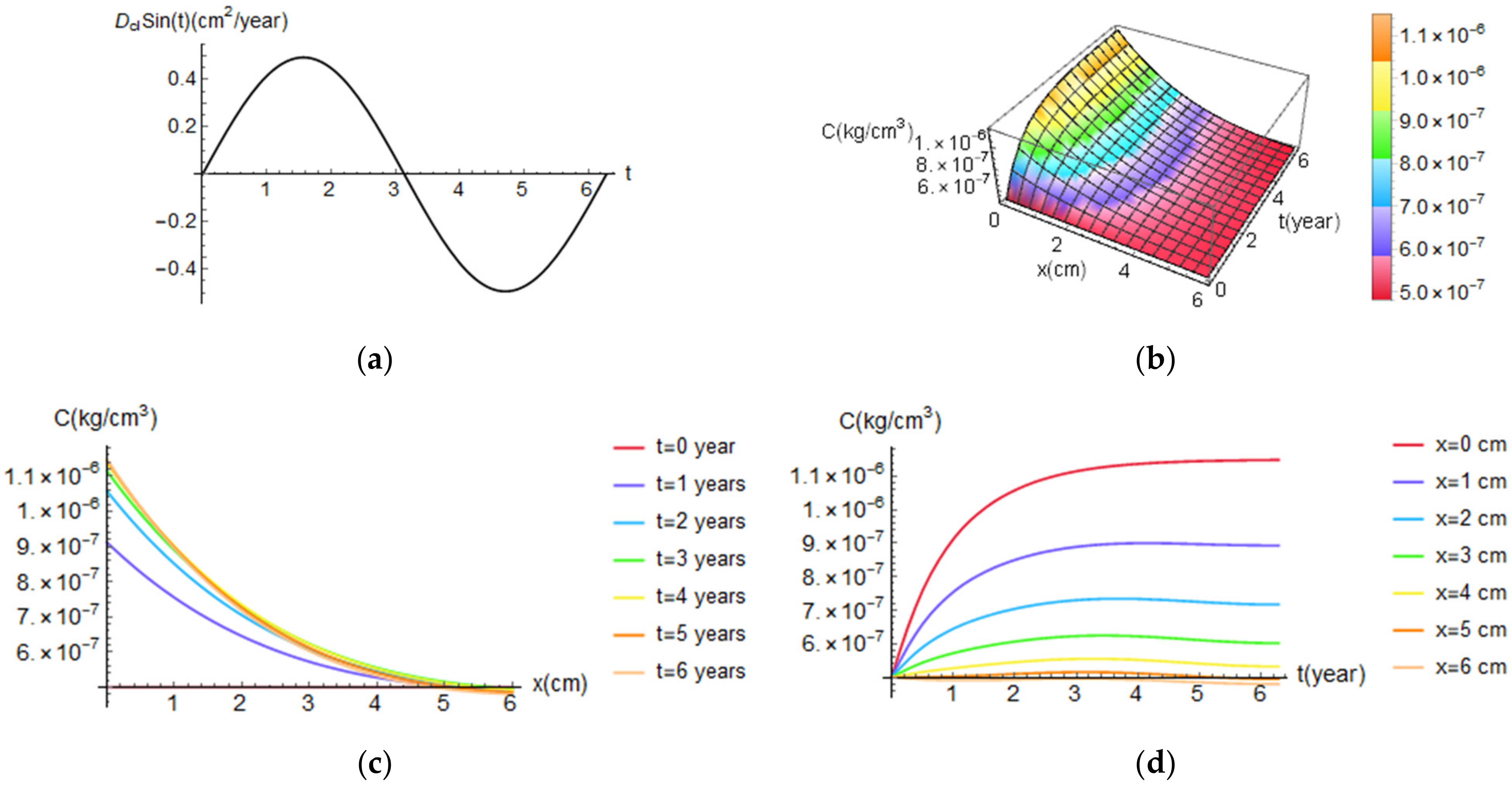
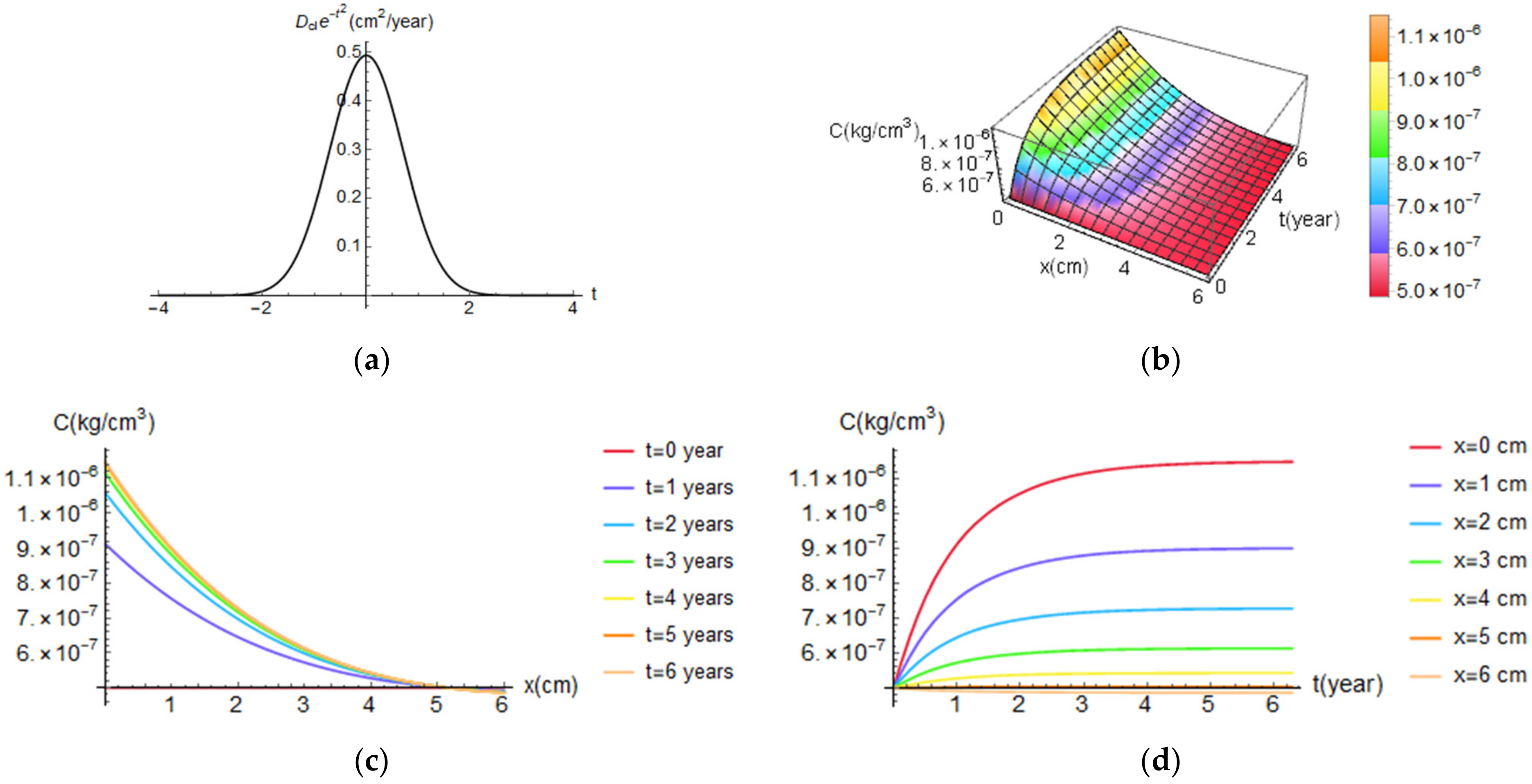
Numerical solutions were developed to study the trend of D_cl under different loadings. Fick’s II law expressed by Equation (2) is a highly non-linear equation hard to accurately solve. Considering D_cl as a non-constant value means to assume the problem as non-linear. These disadvantages make this model less attractive in practice. For this reason, analytical solutions are usually used. In particular, a methodology was proposed where four types of functions are used (Table 4). Results show that, due to the oscillations of the generic function (e.g., sinusoidal and general), the chloride content C can assume lower values with respect to C values for constant diffusivity. The 3D analyses, accounting for the random variability and advanced solutions, show that chloride C can be higher than ~1.50 compared to C by traditional approaches.

The stochastic approach enables the decision-making process during the design phase, maintenance, and repair. Thus, the accurate estimates (probabilistic + numerical) allow anticipating possible problems and predicting solutions or changing project hypotheses as well as to manage resources.

The prediction of the diffusion time can indicate the beginning of the strength reduction of the structural elements. Moreover, the end of the service lifetime could be earlier than estimated.

For this, future research could focus on, e.g., (i) chloride-ingress models considering multiple mechanisms of cracking/corrosion under seismic actions; (ii) revaluation of the RC structures under climate changes; and (iii) estimation of the interdependencies of all factors using artificial intelligence.

References

1. Liu, J.; Ou, G.; Qiu, Q.; Chen, X.; Hong, J.; Xing, F. Chloride transport and microstructure of concrete with/without fly ash under atmospheric chloride condition. Constr. Build. Mater. 2017, 146, 493–501. [Google Scholar] [CrossRef]
2. Farahani, A.; Taghaddos, H.; Shekarchizadeh, M. Prediction of long-term chloride diffusion in silica fume concrete in a marine environment. Cem. Concr. Compos. 2015, 59, 10–17. [Google Scholar] [CrossRef]
3. Bastidas-Arteaga, E.; Chateauneuf, A.; Sánchez-Silva, M.; Bressolette, P.; Schoefs, F. A comprehensive probabilistic model of chloride ingress in unsaturated concrete. Eng. Struct. 2011, 33, 720–730. [Google Scholar] [CrossRef] [Green Version]
4. Pellizzer, G.P.; Leonel, E.D.; Nogueira, C.G. Numerical approach about the effect of the corrosion on the mechanical capacity of the reinforced concrete beams considering material nonlinear models. Rev. IBRACON Estruturas Mater. 2018, 11, 26–51. [Google Scholar] [CrossRef] [Green Version]
5. Zacchei, E.; Bastidas-Arteaga, E. Multifactorial Chloride Ingress Model for Reinforced Concrete Structures Subjected to Unsaturated Conditions. Buildings 2022, 12, 107. [Google Scholar] [CrossRef]
6. Meira, G.R.; Andrade, M.C.; Padaratz, I.J.; Alonso, M.C.; Borba, J.C., Jr. Measurements and modelling of marine salt transportation and deposition in a tropical region in Brazil. Atmos. Environ. 2006, 40, 5596–5607. [Google Scholar] [CrossRef]
7. El Hassan, J.; Bressolette, P.; Chateauneuf, A.; El Tawil, K. Reliability-based assessment of the effect of climatic conditions on the corrosion of RC structures subject to chloride ingress. Eng. Struct. 2010, 32, 3279–3287. [Google Scholar] [CrossRef]
8. Stewart, M.G.; Mullard, J.A. Spatial time-dependent reliability analysis of corrosion damage and the timing of first repair for RC structures. Eng. Struct. 2007, 29, 1457–1464. [Google Scholar] [CrossRef]
9. Al-Kutti, W.A.; Rahman, M.K.; Shazali, M.A.; Baluch, M.H. Enhancement in Chloride Diffusivity due to Flexural Damage in Reinforced Concrete Beams. J. Mater. Civ. Eng. 2014, 26, 658–667. [Google Scholar] [CrossRef]
10. Xie, Y.; Guan, K.; Zhan, L.; Wang, Q. Mechanical Behavior and Chloride Penetration of Precracked Reinforced Concrete Beams with Externally Bonded CFRP Exposed to Marine Environment. Int. J. Polym. Sci. 2016, 2016, 1790585. [Google Scholar] [CrossRef]
11. Zhang, R.; Castel, A.; François, R. Concrete cover cracking with reinforcement corrosion of RC beam during chlo-ride-induced corrosion process. Cem. Concr. Res. 2010, 40, 415–425. [Google Scholar] [CrossRef]
12. Nguyen, P.T.; Bastidas-Arteaga, E.; Amiri, O.; El Soueidy, C.-P. An Efficient Chloride Ingress Model for Long-Term Lifetime Assessment of Reinforced Concrete Structures Under Realistic Climate and Exposure Conditions. Int. J. Concr. Struct. Mater. 2017, 11, 199–213. [Google Scholar] [CrossRef] [Green Version]
13. Zhang, S.F.; Lu, C.H.; Liu, R.G. Experimental determination of chloride penetration in cracked concrete beams. Procedia Eng. 2011, 24, 380–384. [Google Scholar]
14. Rahimi, A.; Gehlen, C. Semi-probabilistic approach to the service life design of reinforced concrete structures under chloride attack. Beton-Und Stahlbetonbau 2018, 113, 13–21. [Google Scholar] [CrossRef]
15. Pang, L.; Li, Q. Service life prediction of RC structures in marine environment using long term chloride ingress data: Comparison between exposure trials and real structure surveys. Constr. Build. Mater. 2016, 113, 979–987. [Google Scholar] [CrossRef]
16. Wang, Q.; Sun, W.; Guo, L.; Gu, C.; Zong, J. Modeling Chloride Diffusion Coefficient of Steel Fiber Reinforced Concrete under Bending Load. Adv. Civ. Eng. 2018, 2018, 3789214. [Google Scholar] [CrossRef]
17. Ortega, N.F.; Robles, S.I. Assessment of Residual Life of concrete structures affected by reinforcement corrosion. HBRC J. 2016, 12, 114–122. [Google Scholar] [CrossRef] [Green Version]
18. Lizarazo-Marriaga, J.; Claisse, P. Modelling chloride penetration in concrete using electrical voltage and current ap-proaches. Mater. Res. 2011, 14, 31–38. [Google Scholar] [CrossRef] [Green Version]
19. Malheiro, R.; Meira, G.; Lima, M.; Perazzo, N. Influence of mortar rendering on chloride penetration into concrete structures. Cem. Concr. Compos. 2010, 33, 233–239. [Google Scholar] [CrossRef] [Green Version]
20. Bastidas-Arteaga, E.; Schoefs, F.; Stewart, M.G.; Wang, X. Influence of global warning on durability of corroding RC structures: A probabilistic approach. Eng. Struct. 2013, 51, 259–266. [Google Scholar] [CrossRef] [Green Version]
21. Zacchei, E.; Nogueira, C.G. 2D/3D numerical analysis of corrosion initiation in RC structures accounting fluctuation of chloride ions by external actions. KSCE J. Civ. Eng. 2021, 25, 2105–2120. [Google Scholar] [CrossRef]
22. Frier, C.; Sorensen, J.D. Stochastic analysis of the multi-dimensional effect of chloride ingress into reinforced concrete. In Proceedings of the 10th International Conference, ICASP10, Applications of Statistics and Probability in Civil Engineering, Tokyo, Japan, 31 July–3 August 2007. [Google Scholar]
23. Zacchei, E.; Nogueira, C.G. Calibration of boundary conditions correlated to the diffusivity of chloride ions: An accurate study for random diffusivity. Cem. Concr. Compos. 2021, 126, 104346. [Google Scholar] [CrossRef]
24. Andrade, C.; Díez, J.M.; Alonso, C. Mathematical Modeling of a Concrete Surface “Skin Effect” on Diffusion in Chloride Contaminated Media. Adv. Cem. Based Mater. 1997, 6, 39–44. [Google Scholar] [CrossRef]
25. Saetta, A.V.; Schrefler, B.A.; Vitaliani, R.V. 2-D model for carbonation and moisture/hear flow in porous materials. Cem. Concr. Res. 1995, 25, 1703–1712. [Google Scholar] [CrossRef]
26. Wu, L.; Wang, Y.; Wang, Y.; Ju, X.; Li, Q. Modelling of two-dimensional chloride diffusion concentrations considering the heterogeneity of concrete materials. Constr. Build. Mater. 2020, 243, 118213. [Google Scholar] [CrossRef]
27. Zhang, X.; Zhao, Y.; Lu, Z. Probabilistic assessment of reinforcing steel depassivation in concrete under aggressive chloride environments based on natural exposure data. J. Wuhan Univ. Technol. Sci. Ed. 2011, 26, 126–131. [Google Scholar] [CrossRef]
28. Yuan, C.; Li, Y.; Chen, X.; Wang, W. Effect of Reinforced Concrete Cracking on Chloride Ion Penetration. MATEC Web Conf. 2015, 22, 04026. [Google Scholar] [CrossRef] [Green Version]
29. Saassouh, B.; Lounis, Z. Probabilistic modelling of chloride-induced corrosion in concrete structures using first- and sec-ond-order reliability methods. Cem. Concr. Compos. 2012, 34, 1082–1093. [Google Scholar] [CrossRef]
30. Verma, S.K.; Bhadauria, S.S.; Akhtar, S. Evaluating effect of chloride attack and concrete cover on the probability of corrosion. Front. Struct. Civ. Eng. 2013, 7, 379–390. [Google Scholar] [CrossRef]
31. Pang, R.; Xu, B.; Zhou, Y.; Song, L. Seismic time-history response ad system reliability analysis of slopes considering un-certainty of multi-parameters and earthquake excitations. Comput. Geotech. 2021, 136, 104245. [Google Scholar] [CrossRef]
32. Pang, R.; Xu, B.; Zhou, Y.; Zhang, X.; Wang, X. Fragility analysis of high CFRDs subjected to mainshock-aftershock se-quences based on plastic failure. Eng. Struct. 2020, 206, 110152. [Google Scholar] [CrossRef]
33. United Nations (UN). Transforming Our World: The 2030 Agenda for Sustainable Development; Technical Report A/RES/70/1; United Nations (UN): New York, NY, USA, 2015; p. 35. Available online: https://sdgs.un.org/2030agenda (accessed on 1 January 2022).
34. Carrara, P.; De Lorenzis, L.; Bentz, D.P. Chloride diffusivity in hardened cement paste from microscale analyses and accounting for binding effects. Model. Simul. Mater. Sci. Eng. 2016, 24, 065009. [Google Scholar] [CrossRef] [PubMed] [Green Version]
35. Andrade, C. Concepts on the chloride diffusion coefficient. In Proceedings of the Third RILEM Workshop on Testing and Modelling the Chloride Ingress into Concrete, Madrid, Spain, 9–10 September 2002. [Google Scholar]
36. Sun, Y.-M.; Liang, M.-T.; Chang, T.-P. Time/depth dependent diffusion and chemical reaction model of chloride transportation in concrete. Appl. Math. Model. 2012, 36, 1114–1122. [Google Scholar] [CrossRef]
37. Fu, C.; Jin, X.; Jin, N. Modeling of chloride ions diffusion in cracked concrete. In Proceedings of the Earth and Space 2010: Engineering, Science, Construction, and Operations in Challenging Environments, Honolulu, HI, USA, 14–17 March 2010; pp. 3579–3589. [Google Scholar]
38. Fan, W.-J.; Wang, X.-Y. Prediction of Chloride Penetration into Hardening Concrete. Adv. Mater. Sci. Eng. 2015, 2015, 616980. [Google Scholar] [CrossRef] [Green Version]
39. Halamickova, P.; Detwiler, R.J.; Bentz, D.; Garboczi, E.J. Water permeability and chloride ion diffusion in Portland cement mortars: Relationship to sand content and critical pore diameter. Cem. Concr. Res. 1995, 25, 790–802. [Google Scholar] [CrossRef]
40. Kong, J.S.; Ababneh, A.; Frangopol, D.; Xi, Y. Reliability analysis of chloride penetration in saturated concrete. Probabilistic Eng. Mech. 2002, 17, 305–315. [Google Scholar] [CrossRef]
41. Chen, W.; Zhang, J.; Zhang, J. A variable-order time-fractional derivative model for chloride ions sub-diffusion in concrete structures. Fract. Calc. Appl. Anal. 2012, 16, 76–92. [Google Scholar] [CrossRef]
42. Wolfram Mathematica; Version 11, Student ed.; Wolfram Research: Champaign, IL, USA, 2017; Available online: https://www.wolfram.com/mathematica/ (accessed on 14 April 2022).
43. Fu, C.; Jin, X.; Ye, H.; Jin, N. Theoretical and Experimental Investigation of Loading Effects on Chloride Diffusion in Saturated Concrete. J. Adv. Concr. Technol. 2015, 13, 30–43. [Google Scholar] [CrossRef] [Green Version]
44. Zacchei, E.; Nogueira, C.G. Chloride diffusion assessment in RC structures considering the stress-strain sate effects and crack width influences. Constr. Build. Mater. 2019, 201, 100–109. [Google Scholar] [CrossRef]
45. Wang, Y.; Wu, L.; Wang, Y.; Liu, C.; Li, Q. Effects of coarse aggregates on chloride diffusion coefficients of concrete and interfacial transition zone under experimental drying-wetting cycles. Constr. Build. Mater. 2018, 185, 230–245. [Google Scholar] [CrossRef]
46. Damrongwiriyanupap, N.; Limkatanyu, S.; Xi, Y. A Thermo-Hygro-Coupled Model for Chloride Penetration in Concrete Structures. Adv. Mater. Sci. Eng. 2015, 2015, 682940. [Google Scholar] [CrossRef] [Green Version]
47. Zofia, S.; Adam, Z. Theoretical model and experimental tests on chloride diffusion and migration processes in concrete. Procedia Eng. 2013, 57, 1121–1130. [Google Scholar] [CrossRef] [Green Version]
48. Kim, Y.Y.; Lee, B.-J.; Kwon, S.-J. Evaluation Technique of Chloride Penetration Using Apparent Diffusion Coefficient and Neural Network Algorithm. Adv. Mater. Sci. Eng. 2014, 2014, 647243. [Google Scholar] [CrossRef] [Green Version]
49. Van Mien, T.; Stitmannaithum, B.; Nawa, T. Simulation of chloride penetration into concrete structures subjected to both cyclic flexural loads and tidal effects. Comput. Concr. 2009, 6, 421–435. [Google Scholar] [CrossRef]
50. Bažant, Z.P.; Najjar, L.J. Nonlinear water diffusion in nonsaturated concrete. Mater. Struct. 1972, 5, 3–20. [Google Scholar] [CrossRef]
51. Ishida, T.; Iqbal, P.O.; Anh, H.T.L. Modeling of chloride diffusivity coupled with non-linear binding capacity in sound and cracked concrete. Cem. Concr. Res. 2009, 39, 913–923. [Google Scholar] [CrossRef]
52. Nogueira, C.G.; Leonel, E.D.; Coda, H.B. Probabilistic failure modelling of reinforced concrete structures subjected to chloride penetration. Int. J. Adv. Struct. Eng. 2012, 4, 10. [Google Scholar] [CrossRef] [Green Version]
53. Michel, A.; Solgaard, A.; Pease, B.J.; Geiker, M.R.; Stang, H.; Olesen, J.F. Experimental investigation of the relation between damage at the concrete-steel interface and initiation of reinforcement corrosion in plain and fibre reinforced concrete. Corros. Sci. 2013, 77, 308–321. [Google Scholar] [CrossRef]
54. Rosenblatt, M. Remarks on a Multivariate Transformation. Ann. Math. Stat. 1952, 23, 470–472. [Google Scholar] [CrossRef]
55. Oliveira, H.L.; Chateauneuf, A.; Leonel, E.D. Probabilistic mechanical modelling of concrete creep based on the boundary element method. Adv. Struct. Eng. 2018, 22, 337–348. [Google Scholar] [CrossRef]
56. Apostolopoulos, C.; Papadakis, V. Consequences of steel corrosion on the ductility properties of reinforcement bar. Constr. Build. Mater. 2007, 22, 2316–2324. [Google Scholar] [CrossRef]
57. Suo, Q.; Stewart, M.G. Corrosion cracking prediction updating of deteriorating RC structures using inspection information. Reliab. Eng. Syst. Saf. 2009, 94, 1340–1348. [Google Scholar] [CrossRef]
58. Dattoli, G. Generalized polynomials, operational identities and their applications. J. Comput. Appl. Math. 2000, 118, 111–123. [Google Scholar] [CrossRef] [Green Version]
59. Martin-Perez, B.; Pantazopoulou, S.; Thomas, M. Numerical solution of mass transport equations in concrete structures. Comput. Struct. 2001, 79, 1251–1264. [Google Scholar] [CrossRef] [Green Version]
60. Homan, L.; Ababneh, A.; Xi, Y. The effect of moisture transport on chloride penetration in concrete. Constr. Build. Mater. 2016, 125, 1189–1195. [Google Scholar] [CrossRef] [Green Version]
61. Zhang, X.; Li, M.; Tang, L.; Memon, S.A.; Ma, G.; Xing, F.; Sun, H. Corrosion induced stress field and cracking time of reinforced concrete with initial defects: Analytical modeling and experimental investigation. Corros. Sci. 2017, 120, 158–170. [Google Scholar] [CrossRef]
Figure 1. Illustration of FORM and MCS methods (adapted from [29]).
Buildings 12 01211 g001
Figure 2. Flowchart of the general methodology.
Buildings 12 01211 g002
Figure 3. Used probability distributions: (a) Normal distribution N(μ, σ2); (b) Uniform distribution U(xmin, xmax); (c) Beta distribution B(α’, β’); (d) Log-normal distribution logX(μ, σ2).
Buildings 12 01211 g003
Figure 4. Results of scenarios I, II, and III. Probability of failure (or CDF) vs. ta (left), and PDFs by three methods (right) (MCS samples with k = 2.0).
Buildings 12 01211 g004
Figure 5. Results for constant fD(x,t): (a) 2D complete results; (b) results in x domain; (c) results in t domain (0 ≤ t ≤ 2π years with steps dt = 1 year, and 0 ≤ x ≤ 6 cm with steps dx = 1 cm).
Buildings 12 01211 g005aBuildings 12 01211 g005b
Figure 6. Numerical results for sinusoidal fD(x,t): (a) its trend; (b) 2D complete results; (c) results in x domain; (d) results in t domain.
Buildings 12 01211 g006
Figure 7. Numerical results for Gaussian fD(x,t): (a) its trend; (b) 2D complete results; (c) results in x domain; (d) results in t domain.
Buildings 12 01211 g007
Figure 8. Numerical results for general fD(x,t): (a) its trend; (b) 2D complete results; (c) results in x domain; (d) results in t domain.
Buildings 12 01211 g008
Figure 9. Numerical solution of the C(x,y,t) for fD(x,y,t) constant: (a) results in y domain; (b) results in x domain; (c) 3D complete results; (d) example of an RC beam (tm = 2π years, 0 ≤ y ≤ 3 cm with steps dy = 0.5 cm, and 0 ≤ x ≤ 6 cm with steps dx = 1 cm. Data refer to scenario I).
Buildings 12 01211 g009aBuildings 12 01211 g009b