Article

Understanding Residential Occupant Cooling Behaviour through Electricity Consumption in Warm-Humid Climate

by
Kumar Biswajit Debnath
*,
David P. Jenkins
,
Sandhya Patidar
and
Andrew D. Peacock
School of Energy, Geoscience, Infrastructure and Society (EGIS), Heriot-Watt University, Edinburgh EH14 4AS, UK
*
Author to whom correspondence should be addressed.
Buildings 2020, 10(4), 78; https://doi.org/10.3390/buildings10040078
Submission received: 21 March 2020 / Revised: 9 April 2020 / Accepted: 15 April 2020 / Published: 19 April 2020
(This article belongs to the Special Issue Building Energy Consumption in the Global South)

Abstract

:
According to the India Energy Security Scenario 2047, the number of residential air conditioner (A/C) units may increase seven-fold by 2037 as compared to 2017. Also, the related energy consumption might increase four times in the next two decades, according to India’s National Cooling Action Plan. Therefore, the study of occupant cooling behaviour is essential to reduce and manage the significant electricity demand, helping to formulate and implement climate-specific cooling policies, and to adopt low-energy and low-cost technologies at mass-market scale. The study aims to analyse residential electricity consumption in order to investigate occupant behaviour, especially for thermal comfort by using space cooling and mechanical ventilation technologies. Among the five climate zones in India, this study focuses on the occupant behaviour in a warm-humid climate using Auroville as a case study, where climate analysis of the past 30 years demonstrated progression towards unprecedented warmer weather in the last five years. In this study, electricity consumption data from 18 households (flats) were monitored for seven months (November 2018–June 2019). The study also elaborated the limitations faced while monitoring and proposed a data filling methodology to create a complete daily profile for analysing occupant behaviour through electricity consumption. The results of the data-driven approach demonstrated the characteristics and complexities in occupant behaviour and insight on the operation of different technologies to attain thermal comfort in residential buildings in an increasingly warming climate.

1. Introduction

Currently, the second-most populous country of the world, India (1.35 billion in 2018) [1] is expected to have the largest population in the world by 2030 [2]. According to the 2011 census data, India’s population was 1.2 billion, and the number of households was 246 million [3]. Under the 2011 average household size (4.9) assumption, there will be 307 million households in 2030. However, another study showed that there could be as many as 386 million households in India [4]. In addition to the population growth, India’s GDP growth—7.3% in 2018 and forecasted to be 7.5% from 2019–2022 [1]—is one of the highest in the world. According to the World Economic Forum, India will become the third-largest consumer market driven by the affluent middle class—168 million upper-middle (44% of total households) and 132 million lower middle (34% of total households)—by 2030 [4].
Furthermore, India has one of the highest cooling degree days (CDD) in the world. The average annual cooling degree days—Madras (3954), Ahmadabad (3514), Hyderabad (3221), Kolkata (3211), Delhi (2881) and Bangalore (2280) [5]—is estimated to be more than 3000 annually. With the high heat due to climate change, the temperature can increase further in many cities by 2100 which will overwhelmingly increase air-conditioning demand in cities in developing countries such as China, India, Indonesia, and Brazil [6]. Therefore, the annual CDD in many Indian cities may increase significantly. However, only 5% of households in India had air conditioners (A/Cs) in 2018, which is substantially lower than that of China (60%) and USA (90%) [7]. There were 293 million households in India in 2018 [4], which means only 14.7 million households had A/C units. In 2017–2018, the total energy consumption for space cooling was approximately 135 TWh, of which 42% (56.7 TWh) was from room A/C units [8]. Also, studies suggest that India has one of the globally highest cooling gaps—approximately 1.1 billion people may be exposed to heat stress—of almost 335 TWh/y for an indoor set point of 26 °C [9]. Therefore, future projections showed that the space cooling energy consumption of India might reach approximately 585 TWh by 2037–2038 [8], which would be 4.3 times higher than that of 2017–2018.
The high population and increased household affluence may lead to a significant rise of A/C unit ownership in India as access to cooling become viewed as an essential tool to provide comfort. The India energy security scenario 2047 suggests that residential A/C units will increase from 21.8 million in 2017—about 8% of the Indian households—to approximately 68.9 and 154.4 million in 2027–2028 and 2037–2038, respectively [10]. In another study, the International Energy Agency (IEA) suggested that India will have 240 million A/C units by 2030 which will reach 1144 million by 2050 [7], which will be a growth of 42 times over that of 2016.
The government of India has already recognised the necessity of cooling as a priority in state and national level by adopting India Cooling Action Plan (ICAP) in 2019. According to ICAP, room A/C will dominate the building sector’s cooling energy consumption, with 50% of the 600 TWh by 2037–2038. Moreover, there will be a significant presence of non-refrigerant based cooling from fans and air coolers (which use evaporative cooling from passing air over water) at around 40%. ICAP set forth several ambitious goals, such as reducing cooling demand across sectors by 20–25% by 2037–2038 [8]. ICAP also aims at improving the A/Cs efficiency and development of sustainable technologies. There has been a successful standard and labelling policy implementation by Bureau of Energy Efficiency (BEE) for improved room A/Cs efficiencies of 35% between 2006 and 2016 (3% annually) [11]. Despite the A/C improvement targets, the success of ICAP might largely depend on reducing the space cooling demand in India.
There were several studies in the past on the residential electricity consumption of India. A survey-based study on the end-use of electricity in 1165 households in the state of Karnataka in India presented the appliance elasticities and ownership of energy-efficient devices [12]. In another study, Filippini, M and Pachauri, S (2004), used an econometric methodology to examine the elasticity of electricity demand in urban Indian households [13]. Also, there were several residential electricity consumption simulations and forecasting studies on India [14,15]. However, very few studies took India’s household-specific data-driven approach to analyse the residential electricity consumption, particularly for analysing cooling behaviour.
The objective of the study was to examine the occupant’s use of cooling technology to attain thermal comfort using a data-driven approach. As the case study, households in Auroville were selected, representing a warm-humid climate from the southern part of India in Tamil-Nadu. For the study, we took the climate for the last 30 years (1989–2019) to investigate climate evolution and occupant behaviour for thermal comfort through electricity consumption and energy audit data. The data monitoring and analysis revealed the missing data issue due to the limitations and challenges described in Section 2.3. Therefore, we present a data-filling methodology to create a complete representative daily profile form incomplete daily data from the other same days of a month. The results of the data-driven approach demonstrate the characteristics and complexities in occupant behaviour and insights on the user practice on different space-cooling and mechanical ventilation technologies to attain thermal comfort in households in an increasingly warming climate. The study will further be used to inform the work of the Community-scale Energy Demand Reduction in India (CEDRI) project.

2. Methodology

There have been different energy quantifying methods—calculation-based [16,17], measurement-based [18,19] and hybrid quantification [20,21]—applied to evaluate the energy performance of existing buildings [22]. Also, several studies investigated the influence of users’ behaviour on building energy performance with multiple approaches such as monitoring, questionnaire surveys and energy audits [23,24]. However, one of the significant challenges found in the previous studies was the collection of reliable and adequate data for energy-related occupant behaviour understanding [24,25]. In this study, the monitoring-based approach—the measurement-based method—was adopted, which was evaluated with an energy audit to understand the occupant cooling behaviour for attaining thermal comfort.
Among the five climate zones in India, this study focuses on the occupant cooling behaviour in a warm-humid climate—using Auroville as a case study—where summer and wintertime temperature can be 25 °C–35 °C and 20 °C–30 °C, respectively, with relative humidity 70–90%. For the analysis, electricity consumption data from 18 households (flats) were monitored for seven months (November 2018–June 2019). The study had four parts: (a) climate analysis, (b) electricity consumption data collection from the monitored households, (c) using a data filling approach to generate representative weekly electricity demand profile for selected households, and (d) demand pattern analysis for cooling for selected households. Here, initially, the climate analysis methodology would be explained. Then the description of the occupancies and appliance ownership of the monitored households would be presented. After that, the data collection and limitation associated with it would be described, and the later part of Section 2 would explain the data-filling methodology.

2.1. Environmental Stress Index (ESI) Analysis

For the climate analysis, the weather data of Auroville for 30 years (1989–2019) were obtained from the Meteoblue database (www.meteoblue.com). Rather than only analysing temperature as a parameter to show the climate change in Auroville, we adopted the methodology of the Environmental Stress Index (ESI) as a measure for climate analysis because ESI takes into account the effect of climatic parameters such as ambient temperature ( T a ), relative humidity ( RH ) and solar radiation ( SR ). The basic methodology of ESI is described in [26], and the equation is as follows:
ESI = 0.63 T a 0.03 RH + 0.002 SR + 0.0054 ( T a × RH ) 0.073 ( 0.1 + SR ) 1
where, T a is the ambient temperature (°C), RH the relative humidity (%), and SR the solar radiation (Wm−2) and also the output unit for ESI is °C.

2.2. Residential Energy Demand Monitoring: Auroville

Auroville is an experimental township (established 1968) in south India, with approximately 3000 population from different countries [27]. Auroville was selected for the study because of being an intentional eco-friendly community; the residents who were more likely to adopt low-energy behaviours evident in [27,28,29,30,31,32]. The case study buildings are located in the north of Matrimandir—a large golden sphere established in the centre of Auroville—in Tamil Nadu, India. Three apartment buildings—Citadine I and II (34 flats) and Inspiration (14 flats)—are being monitored as case studies (Figure 1). 21 and 9 households were chosen to be observed in Citadines and Inspiration, respectively.

2.2.1. Citadines

Twenty-three occupants (mostly living alone and working in Auroville community) lived in the selected 21 dwellings in Citadines. However, the majority of the dwellings had housemaids who work 4–8 h weekly. The monitored households used incandescent (18.2%), compact fluorescent lamp (CFL) (90.9%), light-emitting diode (LED) (63.6%) and T5 with electronic ballast (90.9%) lighting (Figure 2). According to the India Cooling Action Plan (ICAP), there were three types of space-cooling technologies in Indian buildings: refrigerant-based (room A/Cs, chiller system, variable refrigerant flow (VRF) system, packaged direct expansion (DX), non-refrigerant-based (fan, air cooler), and “not-in-kind” (indirect-direct evaporative cooling system, radiant cooling system, solar Vapor Absorption Machine (VAM) system and others) [8]. There were two types of appliances used in the monitored dwellings for attaining thermal comfort—electric fans (in 100% of dwellings) and room A/Cs (9.1%). Another most common household appliance was a refrigerator (100%). In terms of cooking, Citadines had a community kitchen, where most of the residents had their meals. Most of the dwellings used gas cylinders for cooking in general, although a smaller number had electric stoves. There were also some other appliances used in households such as laptops, TV, router, modem, monitor, speaker, blender, iron, oven, kettle and toaster (Figure 2). The majority of the dwellings had single-phase meters for monitoring electricity consumption.

2.2.2. Inspiration

In the case of Inspiration, ten occupants lived in the selected nine dwellings. The household size and working destinations were similar to occupants of Citadines. The significant difference between the occupants in Inspiration with Citadines was in the usage of types of appliances. Three types of lights, incandescent (55.4%), CFL (88.9%), and LED (44.4%), were used in the dwellings of Inspiration. In the case of heating, ventilation, and air-conditioning (HVAC), electric fans (100%) and A/C (11.1%) were used. In general, as with Citadines, most of the dwellings used gas cylinders for cooking. However, one household had an induction stove. In the case of a refrigerator, eight dwellings had one, and one household had two. The other appliances in used in Inspiration were similar to households in Citadines, except 88.9% of households used geysers for hot water in the bathroom (Figure 2). The dwellings had three-phase meters for monitoring electricity consumption.

2.3. Data Collection

Two types of data were collected from the households: general energy audit and metered electricity consumption. The monitored households were audited for the appliance ownership, rated power of the appliances, layout of the households and total monthly electricity consumption. Blink meters (described below) were installed with electric meter readers for initially 20 households, where 11 had three-phase, and nine had single-phase meters to monitor the electricity consumption. The data collection started in July 2018. After three months of the trial period, the three-phase meters showed inaccuracies as the electricity demand in the majority of the households was significantly lower than expected, with low-power features in the demand profile poorly recorded. However, single-phase meters demonstrated more accurate profiles for low consumption dwellings. Therefore, another ten single-phase meters were installed, which made the total number of households monitored to 30. Among those 30 households, 11 households had 3 phase meters, and 19 houses had single-phase meters. The collected data were stored in the cloud via the local cellular network.

2.4. Limitations

During the data monitoring, several limitations and challenges created a significant number of data gaps within the monitored data.
  • Blink meter-based monitoring: the electricity meter usually shows an alternating current (AC) static energy (Wh) consumption of the household, and there is an external light-emitting diode (LED) which “blinks” each time a certain amount of energy is consumed. The single-phase meters were of 16,000 blinks/kWh specification, i.e., 0.06 Wh/blink. In the case of three-phase meters, the blink resolution was 800 blinks/kWh (1.25 Wh/blink). Temporally precise electricity consumption was monitored in each candidate dwelling using blink meters mounted on top of the LED lights. Due to the characteristics of the blink meters, the blink depends on the amount of electricity consumed. For example, in the case of single-phase meters, the data are registered when at least 0.06 Wh was consumed, and one blink occurred; values lower than that would not be visible, and the system will wait to blink until it consumes a minimum 0.06 Wh. As a result, two days of the same household would have a different timestamp. The irregular timestamps made the aggregation or generalization of demand profile for further analysis a challenge without data transformation.
  • Load shedding: there were regular instances of load shedding—deliberate shutdown in part or parts of a power-distribution system to relieve stress on an electricity grid when demand is higher than the supply—in the monitored buildings. Also, the frequency and duration of the load shedding were not homogenous. To counter the issue of load shedding, some buildings in Auroville uses on-site small diesel generators for electricity.
  • Technical issues: the local cellular gateway was also subject to periodic interruptions due to load shedding, which caused gaps in the data collected. In some cases, the network was disconnected due to maintenance by the utility and service provider. The cellular network companies raised another challenge. There were two separate sim-cards for the buildings. As there was lack of specific data plans for the only Internet of things (IoT) systems, the SIM-cards were used with regular data plans, which automatically switch off the service after several months as there were no incoming or outgoing calls in those SIM-cards.
  • Human factors: another major constraint was the human-related factors of people disconnecting power to the cellular gateway connected to the blink meters unknowingly, which caused missing data issues without notifying the project partners. In some cases, the residents of the monitored buildings connected temporary lights in shared spaces to the power plug for the cellular gateway. The project partners had to disconnect the temporary connections and restart the data collection.

2.5. Missing Data Filling

Missing data, in almost all areas of science and engineering, is one of the most common issues faced by experimental researchers. A range of data infilling methods is available in the literature, which includes simple interpolation-based infilling to smart artificial intelligence (AI)-based approaches [34,35,36]. Some of the commonly applied approaches are mean imputation, random imputation, and regression-based approaches that use other related information, and the last value carried forward [37]. For the present study that involved the analysis of high-resolution (1 min) electricity demand data, we developed a logical iteration-based 8-step data-infilling algorithm (The R code was provided as a Supplementary Materials). The infilling data algorithm was strategically designed to meet the research objectives without losing natural (and multiple) periodic components and statistical properties of the dataset. The method developed here should be useful for the more extensive application involving complex stochastic time series, such as high-resolution electricity demand data with inherent complex dynamics due to several overlapping periodic processes occurring at a range of scale and magnitude (phase and amplitude). The iteration-based 8-step data infilling algorithm involved the following stages:
  • Step 1—Recording missing values: This step involved recording missing data points in the raw data by assigning a timestamp and a “Nan” value.
  • Step 2—Recording repeating values: Quite often, raw data contained repeating entries; our algorithm recorded up to 3 consecutive repeating values and removed them to retain a consistent equidistance time series.
  • Step 3—Counting the total number of missing points: This step helped in assessing the overall quality check of raw data and was essential to account for the reliability of the analysis and results. For the present study, most of the dataset had a missing point within the 5–10% range.
  • Step 4—Logical framework for replacing missing values while retaining periodic components: this was achieved as part of a logical argument that electricity consumption patterns remained consistent (with a small element of randomness) over the different weeks due to similar routines and weekly activity patterns. For example, the consumption at a specific time of the day (say, 9:00 a.m.) for a specific day type (say, Monday) should fluctuate within the close vicinity to values noted at the similar time and day type on following or a previous week. The logical framework was implemented as an iterative procedure.
  • Step 5—Infilling missing values in week 1: this step strategically replaced the missing values in the first week using the data from the following week. The missing value was maybe also missing in the 2nd week. In such cases, the algorithm was designed to move forward and scan week 3 to find the relevant value. The process was repeated until all missing data points are infilled in week 1.
  • Step 6—Infilling missing values from Week 2 to the end of the dataset: this step replaced the missing values using the data from the preceding weeks. Following the same analogy as in Step 5 if the missing value was also missing in the subsequent week. In such cases, the algorithm was designed to move forward and scan the week after to find the relevant value. The process was repeated until all missing data points were infilled in the week.
  • Step 7—Ensuring all missing data points were infilled: to ensure all the missing values were infilled in step 5 and 6, the algorithm checked the total number of Nan values. If there were remaining missing values, step 5 and 6 were iteratively run for up to 10 runs (depending on the length of the data set). The iterative process automatically stopped when all the missing data were infilled.
  • Step 8—Final checks: at the end of the iterative process, the algorithm printed the total number of missing values left after ten iterations. Step 8 was essential as in some rare cases, even after ten iterations, some missing points remain. This happened when the value for a particular time/day was consistently missing throughout the dataset. In such cases, users were informed with the remaining number of missing data points which could be infilled by the user (case-by-case) using some other techniques/logical basis and depending on the nature of the study.

3. Results and Discussion

In this section, firstly the climate analysis of Auroville would be discussed, which would be followed by the generation of representative demand profiles as an approach to address the missing data challenge. Finally, the electricity demand would be discussed to analyse cooling behaviour in selected, monitored households.

3.1. Climate: Auroville

To evaluate the climate of Auroville, first, the typical range of ESI was calculated to be 24.1–34.8 °C—based on annual maximum and minimum temperature [38], RH [39] and solar radiation [40]—with the equation described in Section 2.4. Then, the ESI was calculated for 1989–2019 from the obtained dataset. Figure 3A–F demonstrated the ESI in 1989, 2004 and 2019, and the comparative analysis with the different percentile of typical stress index range. Also, Figure 3G showed the evolution of hourly ESI of Auroville for 1989–2019 within the 50th, 75th and 90th percentile of the typical ESI range. The ESI analysis of last 30 years revealed the increased stress index higher than the 75th and 90th percentile since 2013 and 2017, respectively, which never happened in 1989–2013 (Figure 3G). The hourly analysis of 1989, 2004 and 2019 also demonstrated the ESI increase. In 2019, the stress index values were in 75th and 90th percentile, which were not visible during 2004 and 1989 (Figure 3B,D,F). Therefore, the climate analysis suggested elevated and unprecedented environmental stress level in recent times, which were never experienced before in Auroville.

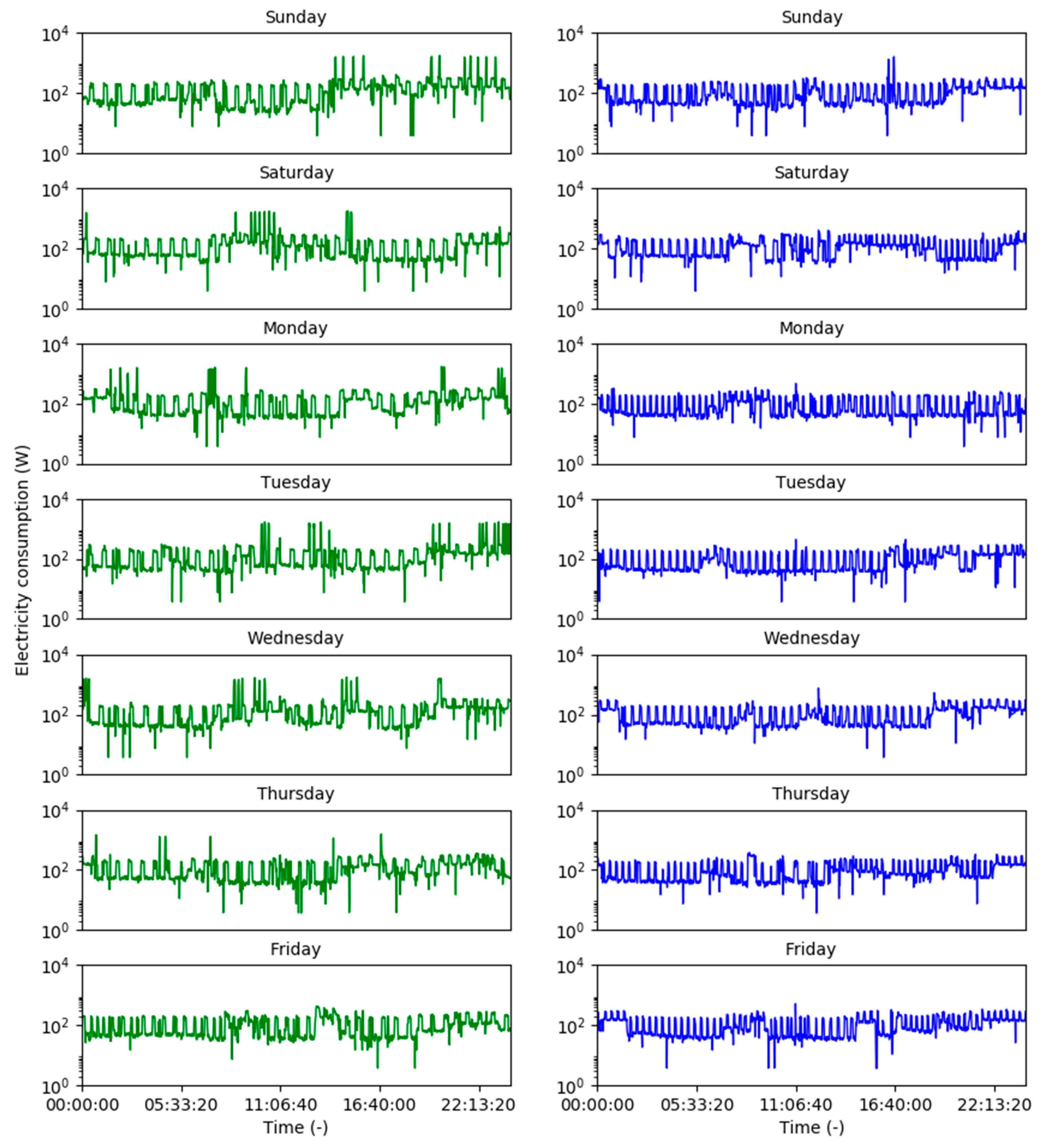
3.2. Electricity Consumption Pattern in Monitored Households with Single-Phase Meters

The majority of the monitored households showed a lower than 350 W of electricity consumption because of the absence of A/C and high power consuming appliances such as hairdryers, electric kettles, and irons. During early November 2018, only five households had more than 350 W of peak electricity consumption out of the 18 monitored households (Figure 4A). Only one household (Home 1) among the five households had an A/C and, therefore, the highest frequency of high electricity features (i.e., spikes in demand) in November. The other electricity consumption spikes in Figure 4A were from high electricity-consuming appliances in the other four households. However, the number of electricity consumption spikes after mid-December 2018 decreased significantly because the A/C usage in ‘Home 1’ household reduced maybe due to the lower air temperature (Figure 4B). Both Figure 3A and Figure 4B showed some gaps in the data due to the limitations and challenges explained in Section 2.4.
The ‘Home 1’ household had one of the highest numbers of high electricity consuming spikes among the combined profiles (Figure 4). The household had a bedroom, a living room, a bathroom, a kitchen and a balcony for one person with an area of 50 m2. The detailed analysis of appliances in the household showed five categories: lighting, HVAC, entertainment and information technology (IT), cooking and food-related, and others. CFL and T5 with electronic ballast were used for lighting. There were three CFLs (18 W) in the living room, one each in the bathroom, balcony and kitchen, respectively. There were three T5 with electronic ballast (14 W) in the bathroom. The household had a 1000 W A/C unit in the bedroom for space cooling. Moreover, there was a 75 W ceiling fan in the bedroom for increasing air change rate. There was also a refrigerator (183 kWh/year), a television (78 W) and an iron (1400 W) in the household.

3.3. Developing a Weekly Profile without Missing Data

The comprehensive analysis of the electricity consumption requires a complete daily dataset, which was not possible in the study due to various limitations described in Section 2.4. For example, Figure 5 (Blue) showed the electricity consumption profile of ‘Home 1’ on 28 days of November 2018. There were missing data for almost every day. Understanding the daily electricity consumption pattern would be somewhat incomplete from the data of Figure 5 (Blue ones). The study utilized the missing data filling methodology described in Section 2.5 to develop a representative electricity consumption profile for each day to circumvent the limitation.
In the case of 3–9 November, the same day of the following weeks was used for the data filling and generating equal timestamps. The green profiles in Figure 5 were the representative profile of the week of 3–9 November, where the incomplete profiles were used as a base, and the missing values were filled in with the data form same day of the next weeks. For example, the synthesized profile of Sunday was obtained from the profiles of 3, 10, 17 and 24 November, which were all Sundays.

3.4. Electricity Consumption Analysis for Comfort in the Selected Household

During the representative profile of 3–9 November in Figure 6 (Green), the household showed three main periods with high electricity consumptions: morning (07:00–11:15), afternoon (12:00–17:00) and night (19:00–01:00). However, during weekdays, the use of high consuming appliances increased at night period. The baseline electricity consumption in the households was around 300 W, and the high demand spikes reached up to 1600–1700 W. Cross-checking the electricity consumption pattern with the appliances ownership of the household suggested that the high demand spikes might have been caused by the use of A/C for cooling and use of Iron. However, the frequency and periods of electricity use suggested that the A/C was the primary cause of high demand.
Moreover, the demand profile during 22–28 December 2018 in Figure 6 (Blue) showed none/minimal use of A/C as the air temperature was on average 27.9 °C, around 3 °C less than that of 3–9 November 2018. At the same time, the highest relative humidity value was 98% (in the weekends), lowest 84% (during weekdays), and average 92%, which may have contributed to the truncated use of A/C. There was only one high demand spike at the weekend, which may have been caused by the use of other appliances. If the high consumption were removed, the demand profile would resemble a household (Home 4) with only fans for attaining thermal comfort (Figure 7). The results of significant difference between households with and without A/C, resembles the outputs from [41], despite the difference in the context of Australia, resolution of data and presence of high electricity-consuming appliances in the households.
Although the ‘Home 4’ household did not have any A/C, it had an oven (1200 W), a refrigerator, a coffee machine (800 W), a kettle (1350 W), and an iron (750 W). The week demonstrated here did not show any use of high consuming appliances (Figure 7). The base demand appeared to exhibit a typical refrigerator profile.
In the case of attaining thermal comfort, two types of user patterns were observed in ‘Home 1’: only an electric fan and A/C with a fan. During the warmer period of November, the comfort was achieved mostly with a combination of A/C and electric fan. The minute analysis in Figure 6 (Green) showed that A/C might be operated for total 2.7% (39 min), 2.6% (38 min), 3.3% (47 min), 4.4% (64 min), 4.09% (59 min), 1.04% (15 min) and 0 min of the day on 3–9 November, respectively. Upon excluding the spikes (more than 500 W) and repetitive cyclic patterns (below 200 W) in the electricity consumption profile of ‘Home 1’, there were 15.34% (221 min), 16.32% (235 min), 15.76% (227 min), 15.56% (224 min), 13.89% (200 min), and 16.18% (233 min) minutes of the day on 3–8 November, respectively, may have been dominated by electric fans especially between the electricity spikes. However, there was no high electricity consumption spike on 9 November and 11.81% (170 min) minutes of the day was between the 200–500 W range, which may be caused by fan operation. On 3–7 November especially at night, the occupant might have used the A/C for some time and then used a fan to circulate the cooled air around the room to reduce the use of high electricity-intensive appliance (Figure 6 Green). The use of space-cooling appliances in ‘Home 1’ reduced in the later period of December (Figure 6 Blue), most probably due to lower temperature and humidity than that of early November. In Figure 6 Blue, approximately less than 100 W increased at night (19:00–02:00), which may be the use of electric fan (75 W in the bedroom) for mechanical ventilation. Although the use pattern of A/C and fan need to be verified by the users, the use of a fan to reduce A/C cooling needs in mixed mode (MM) residential building—buildings in which a combination of air-conditioning and natural ventilation is used to provide thermal comfort—in India can also be found in [42]. Also, another study showed that on average 75% buildings in Asia used a fan for attaining thermal comfort which was higher than that of Europe, America and Australia, and naturally ventilated (NV), and MM buildings had average 82% and 70% fan-use rate, respectively [43]. Although, the fan-use rate was shown to be an average of 57% and 48% in NV and MM buildings in Pakistan, respectively [44], which was lower than that of [43]. One of the reasons for the difference may be the climatic difference, as Indraganti (2010) showed that the use of thermal comfort appliances significantly correlated with outdoor and indoor temperatures in Indian apartments [45]. The occupant behaviour pattern and energy audit of the analysed households in this study showed similar outputs of the use of higher fan-use, although, ‘Home 1’ occupant used A/C and fans, and ‘Home 4’ occupant used a combination of natural ventilation and fans for attaining thermal comfort.
The residential user behaviour for thermal comfort demonstrated some intriguing patterns, which were in contrast to, for example, the UK’s domestic space heating behaviour. User profiles for space heating had a certain degree of homogeneity across most households [46], where the heating was mostly centralised in the dwelling. The residential space conditioning in monitored households in Auroville suggested that fans and A/Cs were separate, room-based appliances, mostly in bedrooms, which meant a more complex and varied relationship between occupancy and technology. Although the electricity demand profiles presented begin to show some correlation between known appliances in the dwelling and space-cooling demand, there might be a need for more detailed qualitative and quantitative data regarding cooling behaviour from the occupants.
The analysed appliance-use behaviours will, in the future, be utilised to generate user profile schedules for appliances in the virtual environment of dynamic simulation models, to investigate the effect of different demand reduction scenarios for the CEDRI project [47]. There is a substantial gap in understanding of residential electricity consumption behaviours in India due to the significant diverse influence of demography, local geography/climate, economy, culture and technological variables and complexities. This study was an initial step towards understanding the electricity use behaviour on a household scale, and to aggregate to a community scale to simulate the effect of different electricity demand-reduction strategies.

4. Conclusions

The objective of the study was to understand the characteristics of occupancies in households to attain thermal comfort in a warm-humid climate—using Auroville as a case study—through the analysis of electricity demand profiles. The electricity consumption profile of 18 households was collected and analysed. There were several issues such as load shedding (power cuts), the human factor (lack of awareness) and technical issue (equipment breakdown) caused some data gaps. We used a data-filling methodology to circumvent the data gap issue and generated complete representative daily electricity consumption profile to analyse the cooling behaviour.
Initially, 30 years’ weather data was obtained to calculate the annual hourly Environmental Stress Index (ESI) for climate analysis. The ESI analysis revealed the unprecedented and rapid increase in environmental stress in the climate of Auroville since 2014. Under the elevated stress, attaining thermal comfort in a warm-humid climate would become challenging with natural ventilation or mechanical ventilation, which might direct the occupants towards using comparatively higher electricity-intensive but available space-cooling technologies.
Moreover, the analysis of the demand profiles demonstrated several intriguing occupancy behaviours. Most of the households used ceiling fans for thermal comfort. Although some households also used A/C for space cooling, they also had ceiling fans for mechanical ventilation too. These households with A/C and ceiling fans did not use A/C continuously for attaining thermal comfort. The demand profile showed that the occupancies might use the A/C to cool the indoor air and fans to circulate the cooled air until it gets warm and then again use A/C. The main reason behind these characteristics might be to reduce the use of an electricity-intensive appliance to minimise the consumption and associated bills.
Further occupancy interviews would reveal the nuances behind this behaviour, but this initial work illustrated that pattern recognition of demand profiles might be useful at characterising usage of cooling and fan technologies in Indian dwellings. It also illustrates that, for purposes of modelling, control assumptions of residential cooling (with different categories of technology used to achieve comfort) are not necessarily analogous to control profiles for heating technologies in colder climates. The complex synergy between increasing air-changes (through increased ventilation) and cooling that air can be challenging to predict—although this study provides the first step to help recognize such activities in high-resolution demand profiles.
The research will further be used to inform the work of the CEDRI project (Grant reference EP/R008655/1) funded by Department of Science and Technology (DST) in India and the Engineering and Physical Sciences Research Council (EPSRC) in the UK, to combine energy network and building modelling with behavioural studies to tailor demand reduction strategies for Indian communities.

Supplementary Materials

The following are available online at https://www.mdpi.com/2075-5309/10/4/78/s1: Infilling_Missing Data_R Code supplementary materials.

Author Contributions

Conceptualization, K.B.D. and D.P.J.; methodology, K.B.D. and S.P.; formal analysis, K.B.D.; investigation, K.B.D.; resources, K.B.D., A.D.P. and S.P.; data curation, K.B.D.; writing—original draft preparation, K.B.D.; writing—review and editing, K.B.D., D.P.J., A.D.P. and S.P.; visualization, K.B.D.; supervision, D.P.J.; project administration, D.P.J.; funding acquisition, D.P.J., A.D.P. and S.P. All authors have read and agreed to the published version of the manuscript.

Funding

This research was funded by the CEDRI project (Grant reference EP/R008655/1) is funded by the Engineering and Physical Sciences Research Council (EPSRC) and Indian Department of Science and Technology as part of the Newton-Bhabha programme.

Acknowledgments

The authors wish to acknowledge the technical support from Martin Scherfler, Jaswanth Yaddala and others of Auroville Consulting (AVC) for the data collection process.

Conflicts of Interest

The authors declare no conflict of interest. The funders had no role in the design of the study; in the collection, analyses, or interpretation of data; in the writing of the manuscript, or in the decision to publish the results.

References

  1. World Bank. World Development Indicators (WDI). 2019. Available online: http://databank.worldbank.org/data/source/world-development-indicators (accessed on 10 November 2019).
  2. United Nations. World Population Prospects 2019. United Nations, 2019. Available online: https://population.un.org/wpp/Graphs/Probabilistic/POP/TOT/156 (accessed on 1 November 2019).
  3. Government of India. HOUSING—Statistical Year Book India 2017. Ministry of Statistics & Programme Implementation, 2017. Available online: http://mospi.nic.in/statistical-year-book-india/2017/197 (accessed on 25 November 2019).
  4. World Economic Forum. Future of Consumption in Fast-Growth Consumer Markets: INDIA; WEF: Cologny, Switzerland, 2019. [Google Scholar]
  5. Sivak, M. Potential energy demand for cooling in the 50 largest metropolitan areas of the world: Implications for developing countries. Energy Policy 2009, 37, 1382–1384. [Google Scholar] [CrossRef]
  6. Sustainable Energy for All. Chilling Prospects: Providing Sustainable Cooling for All; Sustainable Energy for All: Vienna, Austria, 2018. [Google Scholar]
  7. IEA. Energy Efficiency: Cooling. International Energy Agency, 2019. Available online: https://www.iea.org/topics/energyefficiency/buildings/cooling/ (accessed on 1 November 2019).
  8. Government of India. India Cooling Action Plan; Government of India: New Delhi, India, 2019.
  9. Mastrucci, A.; Byers, E.; Pachauri, S.; Rao, N.D. Improving the SDG energy poverty targets: Residential cooling needs in the Global South. Energy Build. 2019, 186, 405–415. [Google Scholar] [CrossRef]
  10. Government of India. India Energy Security Scenarios 2047. Government of India, 2015. Available online: http://iess2047.gov.in (accessed on 1 November 2019).
  11. Abhyankar, N.; Shah, N.; Park, W.Y.; Phadke, A. Accelerating Energy Efficiency Improvements in Room Air Conditioners in India: Potential, Costs-Benefits, and Policies; Ernest Orlando Lawrence Berkeley National Laboratory: Berkeley, CA, USA, 2017.
  12. Murthy, K.N.; Sumithra, G.D.; Reddy, A.K. End-uses of electricity in households of Karnataka state, India. Energy Sustain. Dev. 2001, 5, 81–94. [Google Scholar] [CrossRef]
  13. Filippini, M.; Pachauri, S. Elasticities of electricity demand in urban Indian households. Energy Policy 2004, 32, 429–436. [Google Scholar] [CrossRef] [Green Version]
  14. Van Ruijven, B.; Van Vuuren, D.P.; De Vries, B.J.; Isaac, M.; Van Der Sluijs, J.P.; Lucas, P.; Balachandra, P. Model projections for household energy use in India. Energy Policy 2011, 39, 7747–7761. [Google Scholar] [CrossRef] [Green Version]
  15. Dhar, S.; Srinivasan, B.; Srinivasan, R. Simulation and Analysis of Indian Residential Electricity Consumption Using Agent-Based Models. Softw. Archit. Tools Comput. Aided Process Eng. 2018, 43, 205–210. [Google Scholar]
  16. Al-Homoud, M.S. Computer-aided building energy analysis techniques. Build. Environ. 2001, 36, 421–433. [Google Scholar] [CrossRef]
  17. Vartholomaios, A. A parametric sensitivity analysis of the influence of urban form on domestic energy consumption for heating and cooling in a Mediterranean city. Sustain. Cities Soc. 2017, 28, 135–145. [Google Scholar] [CrossRef]
  18. Räsänen, T.; Voukantsis, D.; Niska, H.; Karatzas, K.; Kolehmainen, M. Data-based method for creating electricity use load profiles using large amount of customer-specific hourly measured electricity use data. Appl. Energy 2010, 87, 3538–3545. [Google Scholar] [CrossRef]
  19. He, D.; Lin, W.; Liu, N.; Harley, R.G.; Habetler, T.G. Incorporating Non-Intrusive Load Monitoring Into Building Level Demand Response. IEEE Trans. Smart Grid 2013, 4, 1870–1877. [Google Scholar]
  20. Widén, J.; Lundh, M.; Vassileva, I.; Dahlquist, E.; Ellegård, K.; Wäckelgård, E. Constructing load profiles for household electricity and hot water from time-use data—Modelling approach and validation. Energy Build. 2009, 41, 753–768. [Google Scholar] [CrossRef]
  21. Reddy, T.A. Literature review on calibration of building energy simulation programs: Uses, problems, procedures, uncertainty, and tools. ASHRAE Trans. 2006, 112, 226. [Google Scholar]
  22. Wang, S.; Yan, C.; Xiao, F. Quantitative energy performance assessment methods for existing buildings. Energy Build. 2012, 55, 873–888. [Google Scholar] [CrossRef]
  23. Yu, Z.; Fung, B.C.; Haghighat, F.; Yoshino, H.; Morofsky, E. A systematic procedure to study the influence of occupant behavior on building energy consumption. Energy Build. 2011, 43, 1409–1417. [Google Scholar] [CrossRef] [Green Version]
  24. Hong, T.; Taylor-Lange, S.C.; D’Oca, S.; Yan, D.; Corgnati, S.P. Advances in research and applications of energy-related occupant behavior in buildings. Energy Build. 2016, 116, 694–702. [Google Scholar] [CrossRef] [Green Version]
  25. Yan, D.; O’Brien, W.; Hong, T.; Feng, X.; Gunay, H.B.; Tahmasebi, F.; Mahdavi, A. Occupant behavior modeling for building performance simulation: Current state and future challenges. Energy Build. 2015, 107, 264–278. [Google Scholar] [CrossRef] [Green Version]
  26. Moran, D.; Pandolf, K.; Shapiro, Y.; Heled, Y.; Shani, Y.; Mathew, W.; Gonzalez, R. An environmental stress index (ESI) as a substitute for the wet bulb globe temperature (WBGT). J. Therm. Boil. 2001, 26, 427–431. [Google Scholar] [CrossRef]
  27. AF. Auroville in Brief. Auroville Foundation, 2017. Available online: https://www.auroville.org/contents/95 (accessed on 1 November 2019).
  28. AF. Auroville Green Practices. Auroville Foundation, 2020. Available online: http://www.green.aurovilleportal.org/ (accessed on 1 November 2019).
  29. Kundoo, A. Auroville: An Architectural Laboratory. Arch. Des. 2007, 77, 50–55. [Google Scholar] [CrossRef]
  30. Kapoor, R. Auroville: A spiritual-social experiment in human unity and evolution. Future 2007, 39, 632–643. [Google Scholar] [CrossRef]
  31. Nagy, B. Experimented methods to moderate the impact of climate change in Auroville. Ecocycles 2018, 4, 20–31. [Google Scholar] [CrossRef] [Green Version]
  32. Loret, S.L.; Martin, S.; Sarkhot, D. Sustainable Energy in Auroville The Vision and the Reality; Indian Institute of Technology Madras: Auroville, India, 2002. [Google Scholar]
  33. Google Maps. Map Showing the Location of Auroville. Google, 2019. Available online: https://www.google.com/maps (accessed on 1 November 2018).
  34. Dumedah, G.; Coulibaly, P. Evaluation of statistical methods for infilling missing values in high-resolution soil moisture data. J. Hydrol. 2011, 400, 95–102. [Google Scholar] [CrossRef]
  35. Khalil, M.; Panu, U.S.; Lennox, W.C. Groups and neural networks based streamflow data infilling procedures. J. Hydrol. 2001, 241, 153–176. [Google Scholar] [CrossRef]
  36. Coulibaly, P.; Evora, N. Comparison of neural network methods for infilling missing daily weather records. J. Hydrol. 2007, 341, 27–41. [Google Scholar] [CrossRef]
  37. Gelman, A.; Hill, J. Data Analysis Using Regression and Multilevel/Hierarchical Models by Andrew Gelman; Cambridge University Press: Cambridge, UK, 2006. [Google Scholar]
  38. Climate-Data. Auroville Climate. 2020. Available online: https://en.climate-data.org/asia/india/tamil-nadu/auroville-31587/ (accessed on 1 January 2020).
  39. Weather Spark. Average Weather in Auroville. Cedar Lake Ventures. 2020. Available online: https://weatherspark.com/y/109814/Average-Weather-in-Auroville-India-Year-Round (accessed on 1 January 2020).
  40. Synergy Enviro Engineers. Solar Irradiance (Puducherry). Synergy Enviro Engineers, 2020. Available online: http://www.synergyenviron.com/tools/solar-irradiance/india/puducherry/puducherry (accessed on 1 January 2020).
  41. Fan, H.; MacGill, I.; Sproul, A. Statistical analysis of drivers of residential peak electricity demand. Energy Build. 2017, 141, 205–217. [Google Scholar] [CrossRef]
  42. Vyas, D.; Apte, M. Effectiveness of Natural and Mechanical Ventilative Cooling in Residential Building in Hot & Dry and Temperate Climate of India. In Proceedings of the 33rd PLEA International Conference: Design to Thrive (PLEA 2017), Edinburgh, UK, 2–5 July 2017. [Google Scholar]
  43. He, Y.; Chen, W.; Wang, Z.; Zhang, H. Review of fan-use rates in field studies and their effects on thermal comfort, energy conservation, and human productivity. Energy Build. 2019, 194, 140–162. [Google Scholar] [CrossRef] [Green Version]
  44. Rijal, H.B.; Humphreys, M.; Nicol, F. Understanding occupant behaviour: The use of controls in mixed-mode office buildings. Build. Res. Inf. 2009, 37, 381–396. [Google Scholar] [CrossRef]
  45. Indraganti, M. Behavioural adaptation and the use of environmental controls in summer for thermal comfort in apartments in India. Energy Build. 2010, 42, 1019–1025. [Google Scholar] [CrossRef]
  46. McCallum, P.; Jenkins, D.; Peacock, A.D.; Patidar, S.; Andoni, M.; Flynn, D.; Robu, V. A multi-sectoral approach to modelling community energy demand of the built environment. Energy Policy 2019, 132, 865–875. [Google Scholar] [CrossRef]
  47. CEDRI. Community-Level Energy Demand Reduction (CEDRI) Project. 2018. Available online: www.cedri.hw.ac.uk (accessed on 1 June 2019).
Figure 1. Monitored buildings (Auroville); source [33].
Buildings 10 00078 g001
Figure 2. Appliance ownership in monitored households.
Buildings 10 00078 g002
Figure 3. Environmental stress index (ESI) analysis for Auroville (1989–2019). Hourly ESI in (A) 2019, (C) 2004, and (E) 1989; thick dotted lines at 34.8 °C and 24.1 °C are the upper and lower values of the typical range of ESI for Auroville; the dotted thinner lines denote 10th, 25th, 50th, 75th, and 90th percentiles (bottom to top) between the typical ESI range. The number of hours in 10th, 25th, 50th, 75th, and 90th percentile in (B) 2019, (D) 2004 and (F) 1989. (G) Total hours in top 50th, 75th and 90th percentile of typical ESI range between 1989 and 2019 for Auroville.
Buildings 10 00078 g003
Figure 4. (A) Electricity consumption from 3–9 November 2018; (B) Electricity consumption from 22–28 December 2018.
Buildings 10 00078 g004
Figure 5. (Blue) electricity consumption data of November 2018; (Green) representative electricity consumption profiles for the week of 3–9 November 2018.
Buildings 10 00078 g005
Figure 6. Daily representative electricity demand profile for ‘Home 1’ with air-conditioner (A/C) ((Green) 3–9 November 2018, (Blue) 22–28 December 2018).
Buildings 10 00078 g006
Figure 7. Daily representative electricity demand profile for ‘Home 4’ without A/C ((Green) 3–9 November 2018, (Blue) 22–28 December 2018).
Buildings 10 00078 g007

