
Review

Fatigue Crack Growth Models Applied to Additively Manufactured Electron Beam Melted Ti6Al4V: A Review

Department of Mechanical Engineering, University of Washington, Seattle, WA 98195, USA
*
Author to whom correspondence should be addressed.
Metals 2026, 16(4), 440; https://doi.org/10.3390/met16040440
Submission received: 18 March 2026 / Revised: 10 April 2026 / Accepted: 14 April 2026 / Published: 17 April 2026

Abstract

This article comprehensively reviews the fatigue crack growth (FCG) models applied to Ti6Al4V alloy manufactured by electron beam melting (EBM) powder bed fusion (PBF). The current progress in FCG analytical and numerical models and their application to EBM Ti6Al4V are reviewed. Much experimental data for the creation of historical FCG models was based on conventionally manufactured (CM) aluminum alloys and various steels. With the growth of additive manufacturing (AM), recent studies have applied traditional models and modified new models to EBM Ti6Al4V and validated their use as accurate predictive models for the da/dN-ΔK curve and ΔKth. Due to pores and surface roughness inherent in AM and the unique anisotropic microstructure developed from the EBM process, classical models may require modifications to accurately predict FCG of EBM Ti6Al4V.

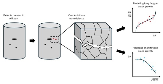
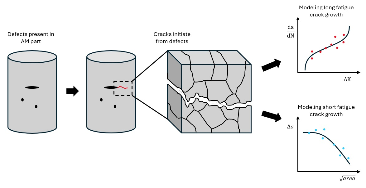
Graphical Abstract

1. Introduction

With the rapid growth of metal additive manufacturing (AM), many industries have shown interest in incorporating it as a standard manufacturing method due to its benefits, including printing near net shape, building complex geometries, and reducing the part count by combining multiple parts into one. These benefits of AM can result in high cost and weight savings. Ti6Al4V is a titanium alloy known as the “workhorse” of the aerospace industry due to its high strength-to-weight ratio, good corrosion resistance, and superior properties that balance strength and ductility. One of the most widely used AM processes is a powder bed fusion (PBF) process called electron beam melting (EBM).
One major hurdle to fully incorporating EBM Ti6Al4V into the aerospace industry is the uncertainty concerning its damage tolerance (DT) with respect to fatigue cracks. Fatigue cracks tend to initiate from manufacturing/material discontinuities (grooves, scratches, burrs, tears, surface treatments, porosity, etc.) [1]. By predicting the rate of fatigue crack growth, DT design allows a certain degree of damage to a structure before repair/replacement is required. One of the reasons fatigue cracks remain a major cause of structural failures in aircraft [2] is that “short cracks” initiate from these defects, whereas many FCG models are based on “long-crack” testing standards (e.g., ASTM E647 [3]). Short cracks are known to grow more quickly than long cracks [4,5,6,7], so the threshold stress intensity factor (SIF) range for long cracks (ΔKth) may not be an applicable threshold for the actual onset of crack growth.
With the advancement of analytical models and computational methods, there has been significant research interest in developing a model that can accurately predict the FCG of AM parts specifically for DT analysis. Due to the history of FCG models and their relationship to the aerospace industry, much experimental data for the creation of traditional models were based on aluminum alloys and various steels and may have been recorded before more sophisticated crack-growth-measuring techniques were available [8]. With the growth of AM and the accumulation of FCG data, recent studies have used traditional models and developed new modified models to apply them to AM metals, including EBM Ti6Al4V [5,9,10,11,12,13,14,15,16,17,18,19,20,21,22,23,24,25,26]. The aim of this review is to bridge classical fracture mechanics with the unique challenges of AM to better predict the FCG of EBM Ti6Al4V for widespread use in industrial applications.

2. Electron Beam Melting Process

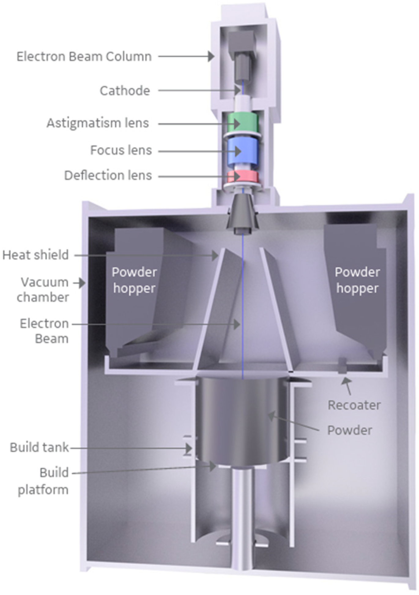
This review focuses on Ti6Al4V built by EBM, which is a PBF AM process that uses an electron beam as the heat source to enact the layer-by-layer process. Figure 1 shows an Arcam A2X EBM machine (Mölndal, Sweden). EBM manufacturing is commonly associated with producing titanium parts, partly due to its increased build chamber gas temperature of 750 °C, which acts as an annealing step that allows parts to be built with negligible residual stresses to reduce part warping. The EBM chamber is maintained in a near-vacuum environment (pressure < 5 × 10⁻⁴ mbar) with a small amount of helium gas added to prevent oxidation and ensure charge neutralization.
However, the EBM process faces some unique AM challenges regarding final part quality. Due to the relatively large powder size of 45–105 μm, EBM-produced parts have a higher surface roughness. Defects are also present in the as-built part, typically gas-induced or lack-of-fusion (LOF) pores [27]. Gas-induced pores are formed when gas is entrapped within the powder during the gas atomization process used for powder production. LOF pores are caused by suboptimal process parameters when the beam energy is insufficient to complete powder melting, resulting in a non-spherical pore that is elongated along a single powder layer. Surface roughness and defects inherently present in as-built EBM parts motivate the use of DT and FCG modeling to predict crack growth and prevent catastrophic failure of components.

3. FCG Models

With the introduction of fracture mechanics concepts in the 1950s, many FCG models were developed from linear elastic fracture mechanics (LEFM) assumptions. Under LEFM, the plastic zone at the crack tip is considered small relative to the size of the specimen; therefore, small-scale yielding (SSY) and bulk elastic behavior can be assumed. Because this is the simplest and most straightforward way to model FCG, much of the available data and models used in the literature use LEFM assumptions to predict crack growth and the determination of ΔKth for long and short cracks.

3.1. da/dN-ΔK Curve

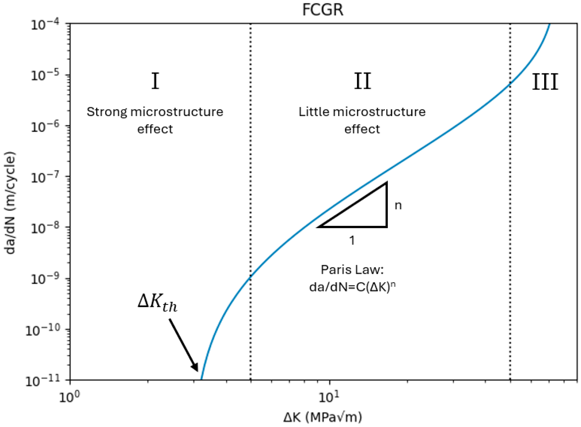
The log–log da/dN-ΔK curve is the most widely used illustration of FCG, which includes the near-threshold Region I, steady crack growth Region II, and overload Region III, shown in Figure 2.
This curve uses the SIF range (ΔK) as the crack driving force, which is derived from linear elastic stress fields and is defined as
Δ K = Y Δ σ π a
Δ K = K m a x K m i n
where Y is a constant geometry factor (Y = 0.65 for surface cracks and Y = 0.5 for internal cracks), Δσ is the applied load, and a is the crack length. The da/dN-ΔK curve was an important contribution because it implied that the crack growth rate is only dependent on ΔK (geometry, load, and the crack length). The simplicity of this curve influenced the development and evolution of many future analytical models with slight variations, many of them attempting to capture the non-continuum FCG behavior in Region I and short-crack growth. A table summarizing each of the discussed FCG models, including the region they apply to, is shown in Table 1.
Proposed in 1963, the Paris law [28] is still extensively used for first-order fatigue life predictions when limited data is available. It is commonly used because of its simplicity; it only requires two parameters (C and m) that are easy to obtain by curve-fitting with experimental data:
d a d N = C ( Δ K ) m
The Paris law uses a power law relationship to describe the steady crack growth behavior in Region II of the da/dN-ΔK curve on a log–log scale, where the two parameters, C and m, are empirically fit as the y-intercept and slope of the curve, respectively. The Paris law is the foundation for many future adaptations of da/dN-ΔK FCG modeling. However, although widely used and a good representation of Region II behavior, it neglects the near-threshold Region I and the overload Region III. It also does not consider stress ratio (R) effects, and there is no physical meaning behind the C and m constants; they are simply representative of the curve-fitting technique used.
In 1967, to address two of these limitations, Forman [29] adapted the Paris law to include the overload Region III and consider stress ratio effects. The Paris law was divided by a factor that approaches 0 as ΔK increases to a critical level Kc (fracture toughness):
d a d N = C ( Δ K ) m ( 1 R ) K c Δ K
While Forman’s contribution included Region III, in 1972, Klesnil and Lukas [33] introduced an equation to model ΔKth in Region I. This equation was based on a power law formulation like the Paris law but did not include Region II–III and only modeled Region I:
d a d N = C ( Δ K m Δ K t h m )
Focusing on Region I, Elber [30] introduced the concept of crack closure in 1970, stating that below a certain “opening” SIF (Kop), where the crack faces are not in contact, there is no crack growth. Therefore, Elber introduced an effective SIF range ΔKeff that can be substituted into Paris Equation (3):
Δ K e f f = K m a x K o p
d a d N = C ( Δ K e f f ) m
Elber further proposed a crack closure ratio U:
U = Δ K e f f Δ K
d a d N = C ( U Δ K ) m
The three types of crack closure effects include plasticity, roughness, and oxide-induced, and they have been used to explain the influence of stress ratio on FCG and the faster crack growth rates of short cracks that do not experience crack closure effects. Closure effects are mostly present in Region I, where ΔKth decreases with increasing stress ratio [10,19,35,36]. It is also observed that closure effects are minimal at higher stress ratios above R = 0.5 [37].
Based on FEA observations, Newman [38] defined a crack closure function f, which is the effective stress ratio when crack closure effects are considered:
f = K o p K m a x
The most common method for obtaining Kop is the adjusted compliance ratio (ACR) method, which is included in the FCG standard testing procedure, ASTM E647 [3].
In 1970, Walker [31] proposed a modification to the Paris law by adding the influence of stress ratio. They defined a new ΔK that accounts for stress ratio and allows all ΔK data to result in the same line after curve-fitting for an empirical constant γ:
d a d N = C [ Δ K ( 1 R ) 1 γ ] m
The empirical constant γ is a material constant that indicates how strongly the stress ratio affects crack growth rate. For many traditional metals, γ = 0.5 but can range from 0.3 to 1.0.
Although Walker’s contribution considered stress ratio effects, this equation still only applied to Region II. Adding a third empirical parameter that requires data from many different stress ratios makes the equation more complicated. However, at this point, the crack growth rates of Regions II and III were able to be predicted accurately with the models available.
To combine Regions I–III into a single model, in 1970, Hartman and Schijve [32] made empirical corrections to the Region I and Region III terms from Walker’s Equation (11). Observing that crack growth was slower in Region I, they suggested that da/dN should be related to how much ΔK exceeds the threshold value so that ΔK − ΔKth is in the numerator. Similarly, observing that crack growth was faster in Region III, they included the rapid acceleration in the denominator as Kmax approaches Kc. They further replaced Kc with the max cyclic fracture toughness (A). (A = Kmax,c = Kmin,c/ΔKc). The modified equation becomes
d a d N = D [ Δ K Δ K t h ( 1 K m a x / A ) q ] p
where D and p become the y-intercept and slope curve-fitting parameters, respectively, which are determined relating da/dN with this new modified crack driving force. This equation produces a sigmoid shape, where the curve steepens at both low and high ends and includes Regions I–III on the da/dN-ΔK curve. The drawback of this model is that ΔKth is sensitive to the stress ratio and that the value of ΔKth must already be known.
The Hartman–Schijve equation was later simplified by using Schwalbe’s [39] crack driving force, where the constant q = 1/2. Further, Jones [34] altered the threshold value as an “apparent threshold SIF range” (ΔKthr) that can be applied to both short- and long-crack threshold values:
Δ κ = Δ K Δ K t h r 1 K m a x A
This gives a modified Hartman–Schijve variant equation using the Schwalbe factor:
d a d N = D ( Δ κ ) p
The NASGRO equation is used in several FCG computer programs (NASGRO, AFGROW, and FASTRAN) and is widely used in the aerospace industry to compute the operational life of a component. Developed by NASA in the 1990s, the NASGRO equation was based on a combination of the abovementioned equations to model Regions I–III:
d a d N = C ( 1 f 1 R ) m Δ K ( m r ) ( Δ K Δ K t h ) r ( 1 K m a x A ) q
where r and q are curve-fitting constants (r controls the lower Region I part of the curve, and q controls the upper Region III part of the curve), and f is the Newman crack closure function from Equation (9) (when crack closure is not present, f = R and the (1 − f)/(1 − R) term cancels out).
The Hartman–Schijve variant Equation (14) and the NASGRO Equation (15) both model FCG in Regions I–III. In addition to analytical models, numerical simulations have also been used to predict FCG.

3.2. Numerical Simulations

Numerical simulations have obvious advantages for FCG prediction due to the time frame of experimental fatigue testing, especially in the near-threshold Region I. Finite element methods (FEM) are commonly used to predict FCG, time to failure, and crack interaction with the microstructure.
In 1981, Newman [38] used FEA to observe plasticity-induced crack closure and proposed the strip-yield model to reproduce results more computationally efficiently. The strip-yield model predicts plasticity-induced crack closure and ΔKeff in FCG and is the basis for NASGRO’s closure model. The model uses bars of a rigid plastic material surrounding the crack. Region 1 is an elastic continuum, Region 2 is modeled with the perfectly plastic material mimicking the plastic zone, and Region 3 is in the wake of the crack, which uses the same plastic material, but the elements are split and can only transfer compressive (not tensile) loads.
An extension to traditional FEM is the extended FEM (XFEM) proposed in 1999 [40]. XFEM takes advantage of the partition of unity property of finite elements, which allows enrichment functions to be added to the finite element shape function that approximates the behavior between two nodes. The enrichment function allows a specific approximation in a region of interest.
In 2017, ref. [41] proposed the use of the plastic component of the crack tip opening displacement (CTOD) as the nonlinear parameter that replaces ΔK to create a da/dN-CTODp curve. They used FEA to simulate a strain-life curve using experimental data from low-cycle fatigue (LCF) tests, separated the elastic and plastic regions of the CTOD, and used the plastic portion, CTODp. This method addresses the drawback of using ΔK as the crack driving force because it does not capture the nonlinear, elastic–plastic behavior of the crack tip in Region I [41,42].
Another recent numerical simulation popular in the literature is peridynamics (PD), developed by Silling in 2000 [43]. In contrast to traditional continuum mechanics, which use partial differential equations, PD uses integral equations, meaning that they do not require spatial derivatives and are able to handle discontinuities like damage, fracture, and crack growth. PD was developed in 2000 as a “bond-based” model that assumed forces between two bonds are pairwise and symmetric and the material response is linear elastic and isotropic.
In 2010, PD was extended to a “state-based” model that was able to evaluate multiple bonds collectively within a neighborhood, and material response could be anisotropic and plastic [44]. By 2014, PD was applied to FCG, as it was particularly useful for modeling discontinuities like crack growth [45]. The PD equation is a reformulation of Newton’s law F = ma, where the right-hand side is the force and the left-hand side is the mass and acceleration terms:
ρ ( x ) u ¨ ( x , t ) = H x f ( u ( x , t ) u ( x , t ) , x x ) d V x + b ( x , t )
where x is the position of a point, x′ is the position of a neighboring point, ρ (x) is the mass density at point x, u ¨ (x,t) is the acceleration of the material at point x and time t, Hx is the “horizon” (i.e., all nearby points x′ within a certain radius), u(x′,t) − u(x,t) gives the relative displacement between x′ and x, x′ − x is the relative position between x′ and x, and b(x,t) are external body forces. The function defines the force between two points depending on their relative displacement and position and integrates over the horizon for the entire neighborhood of points. Instead of observing the interaction between only two points, PD integrates all the points within a horizon [45]. Ultimately, based on Paris law, the PD relationship is
d a d N = λ B ε c o r e m
where A is a positive parameter and ε c o r e is the bond strain, referring to the bond at the crack tip on the verge of breaking. m is the same value as the Paris exponent from Equation (3).
In addition to predicting FCG, the ΔKth value in Region I is the threshold below which long cracks do not propagate. However, as mentioned earlier, short cracks grow at a faster rate than long cracks, meaning that short cracks may propagate below this threshold. Many models have focused on predicting ΔKth for long and short cracks.

3.3. Predicting ΔKth

With standard long-crack FCG testing procedures, the determination of ΔKth requires many specimens to account for variability, making it expensive and time-consuming. Further, the ASTM E647 standard simply defines ΔKth as the ΔK value when da/dN is extrapolated to approximately 10−10 m/cycle on the log–log da/dN-ΔK curve using a K-decreasing test method. This method also does not consider short-crack growth below the ΔKth value. Due to these reasons, many models have been developed analytically or empirically to approximate ΔKth for long and short cracks.
Short cracks can be categorized as “microstructurally small”/”microcrack” or “physically small”. Table 2 below defines approximate size ranges of short and long cracks. Table 3 summarizes each of the discussed ΔKth models and indicates which type of crack size they apply to.
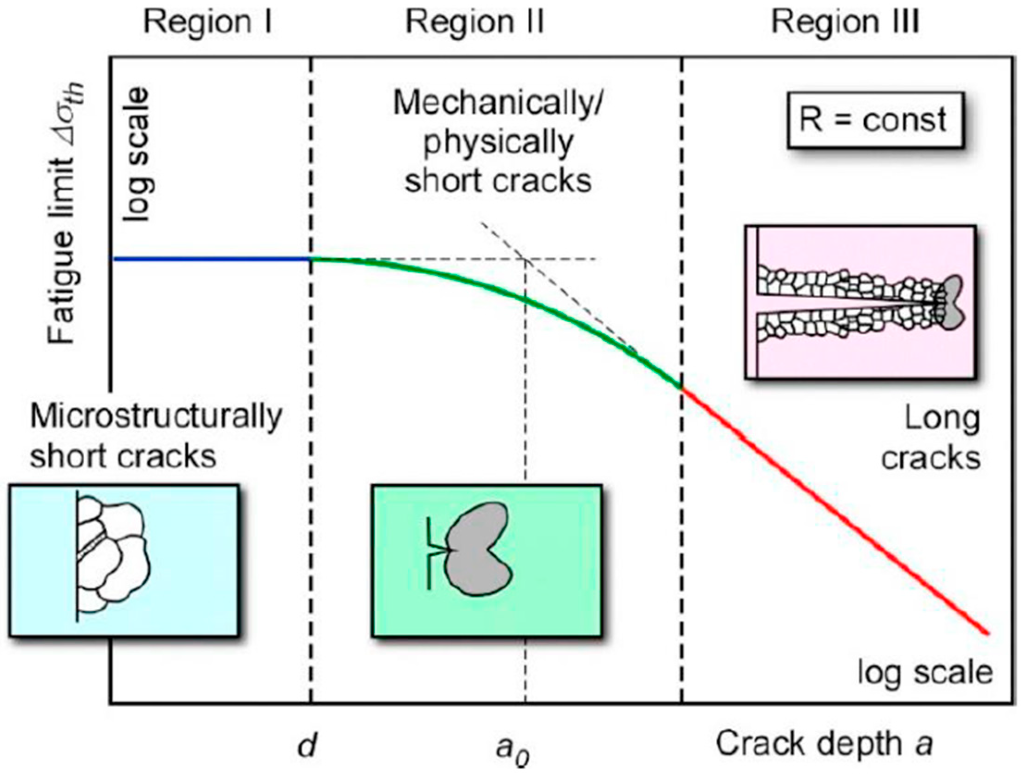
In order to satisfy DT requirements, it is necessary to predict short-crack growth that can initiate from manufacturing/material flaws. The slip mechanism for fatigue crack initiation and FCG is the same. This allows the fatigue limit of “defect-free” specimens (Δσe) from S-N data to be related to the threshold value (ΔKth) from FCG data. When Δσe and ΔKth are known, they can be related by the Kitagawa–Takahashi diagram (KT diagram) [48], which plots the fatigue strength (Δσth) against the crack length (a) on a log–log scale. This relationship provides either the fatigue strength of a specimen when a defect is present or the max allowable crack size for a given applied load. Figure 3 shows a KT diagram with three zones that are associated with microcracks (Zone 1), physically short cracks (Zone 2), and long cracks (Zone 3). This plot shows that fatigue strength diminishes as the crack length increases (d1 is the length of the microcrack threshold, and d2 is the length of the long-crack threshold).
In this diagram, Zone 1 and Zone 3 are easily known, where Zone 1 can be approximated as the defect-free fatigue limit:
Δ σ t h = Δ σ e
Δσe is plotted as a horizontal line in Zone 1. Zone 3 is estimated by the threshold SIF range from Equation (2):
Δ σ t h = Δ K t h π a
ΔKth is plotted with a slope of −1/2 in Zone 3 due to its exponent from the square root in the denominator. Both of these lines from Equations (18) and (19) intersect at a point ao. Introduced in 1979, the El-Haddad [46] parameter ao describes the theoretical defect size that does not affect fatigue strength:
a o = 1 π ( Δ K t h Δ σ e ) 2
However, realistically, the behavior around this point is not linear. There are three popular methods for approximating this nonlinear behavior in Zone 2: El-Haddad’s approach [7,46], the cyclic R-curve method [17,35], and Murakami’s a r e a parameter [47].
Based on the KT diagram, El-Haddad defined a fictitious crack length a + ao to express a continuous curve. Since Zone 2 applies to short cracks, ΔKth,SC is used, so Equation (19) is modified as
Δ σ t h = Δ K t h , S C π ( a + a o )
Rearranging Equation (20), ΔKth,SC is substituted into Equation (21) to approximate Δσth as a function of Δσe, a, and ao:
Δ σ t h = Δ σ e a o a + a o
Similarly, ΔKth,SC is
Δ K t h , S C = Δ K t h a a + a o
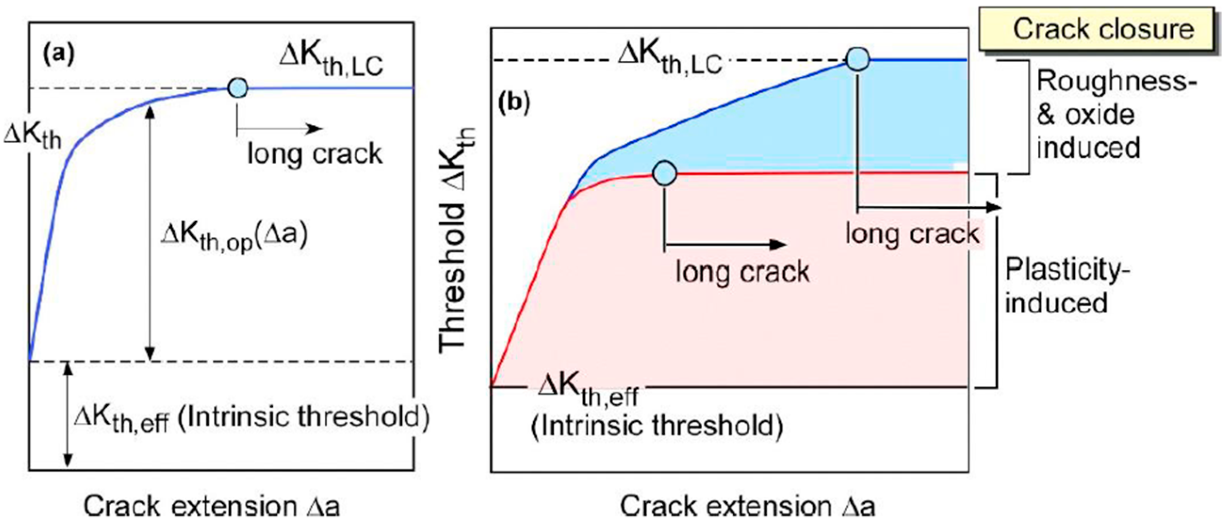
In 1988, Tanaka and Akiniwa [35,49] introduced the cyclic resistance curve (R-curve). While the KT diagram relates short- and long-crack fatigue limits Δσth and uses crack length a, the R-curve relates short- and long-crack ΔKth and uses crack extension Δa. The R-curve method is obtained experimentally by incrementally increasing the applied load until the crack arrests at each load step. This allows multiple data points to be obtained from a single specimen and leads to the curve shown in Figure 4, where the data approach a ΔKth value as crack extension (Δa) increases. This curve assumes crack closure buildup as the main mechanism for FCG resistance. In this context, a material has an intrinsic threshold ΔKth,eff that is material-dependent and an extrinsic threshold ΔKth,op that is affected by factors such as microstructure, stress ratio, and environment. Given an applied load, a crack of a certain length will arrest (below the R-curve) or propagate (above the R-curve).
The information presented by the R-curve is synonymous with that of the KT diagram; it is possible to plot the KT diagram from the R-curve and vice versa since they both provide information about crack arrest loads.
In 2002, Murakami [47] determined that the fatigue limit Δσth is the same as the threshold stress where small cracks do not propagate ΔKth,SC. Therefore, Murakami’s a r e a parameter [50] can be applied to the SIF range Equation (1) by replacing the crack length a with a r e a and replacing ΔK applied to short cracks and Δσ with the fatigue limit:
Δ K t h , S C = Y Δ σ t h π a r e a
Equation (24) can be rearranged to solve for the initial defect size:
a r e a o = 1 π ( Δ K t h , S C Y Δ σ t h ) 2
Substituting and rearranging Equations (24) and (25) solves for ΔKth,SC in terms of a r e a :
Δ K t h , S C = Δ K t h a r e a a r e a + a r e a o
From tests on 16 different materials (various steels, aluminum, and brass annealed, quenched, or tempered) at R = −1 with different-sized small artificial defects, a positive linear relationship between ΔKth,SC and a r e a on a log–log scale, with a slope of 1/3, was found for all 16 materials [47]; this leads to a proportional relationship between the two variables:
Δ K t h , S C ( a r e a ) 1 3
Because the use of a r e a implies short cracks/small defects, the relationship above only applies to a r e a < 1000 µm. Additionally, it was concluded that materials with higher Vickers hardness (HV) had higher ΔKth,SC values. Using a least squares regression method on the 16 different materials, constants were obtained such that:
Δ K t h , S C = 3.3 × 10 3 ( H V + 120 ) ( a r e a ) 1 3
where ΔKth,SC is in MPa m , HV is in kgf/mm2, and a r e a is in µm. Similarly, for the fatigue strength based on two types of carbon steel, on a log–log scale, there was a negative linear relationship between Δσth and a r e a with a slope of −1/6, forming the following relationship:
σ t h ( a r e a ) 1 6
Similarly, using a least squares regression method to solve for constants gives the following relationship:
σ t h = 1.43 ( H V + 120 ) ( a r e a ) 1 6
Equations (28) and (30) are only valid for HV ≤ 400 because the experimental data showed a drastic drop in fatigue limit due to the presence of small defects and larger scatter in the data around HV > 400 [47]. Another empirical formula developed for HV < 400 is only in terms of HV and gives the ideal (“defect-free”) upper bound fatigue limit:
σ e = 1.6 H V ± 0.1 H V
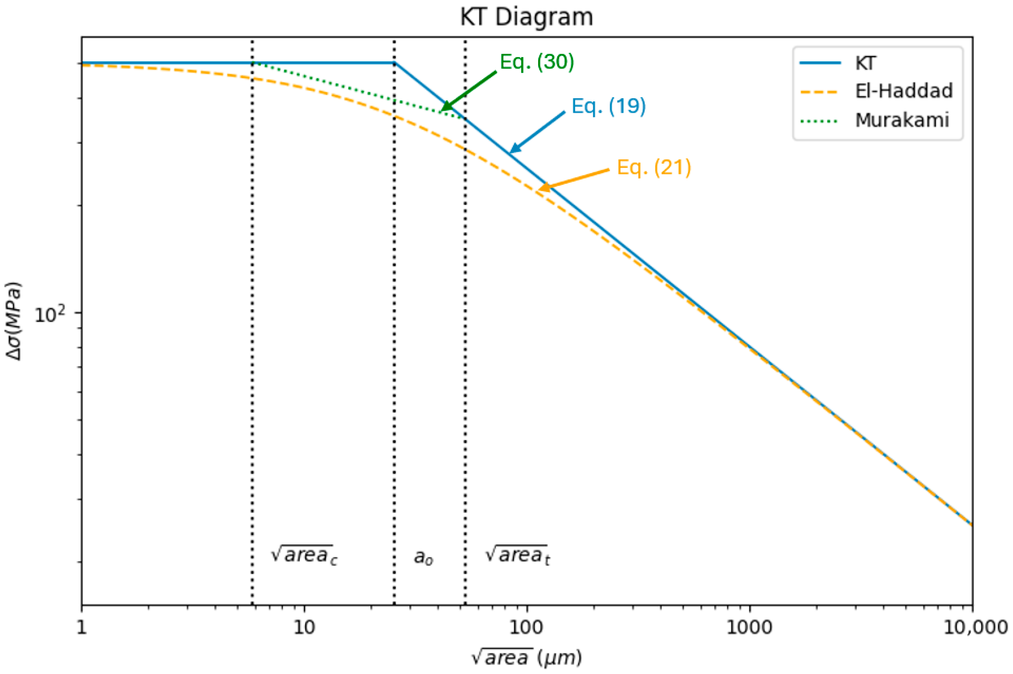
Building on Murakami’s a r e a parameter method, Rigon and Meneghetti [23] used a a r e a approach to solve for the transition defect sizes on the KT diagram (Figure 5). They defined a critical a r e a c between Zone 1 and 2 and a transition a r e a t between Zone 2 and 3. a r e a c is obtained by replacing the fatigue limit in Equation (30) with the defect-free fatigue limit in Equation (31):
a r e a c = ( 1.43 ( H V + 120 ) 1.6 H V ) 6
a r e a c is the max defect size before it becomes damaging. a r e a t is obtained by replacing ΔKth,SC in Equation (28) with the long-crack threshold ΔKth to find the transition defect size between a short and long-crack:
a r e a t = ( Δ K t h 3.3 × 10 3 ( H V + 120 ) ) 3
These values a r e a c and a r e a t are used to define the transition defect size, shown in Figure 5.
Figure 5. KT diagram showing critical a r e a c and transition a r e a t defect sizes.
Metals 16 00440 g005
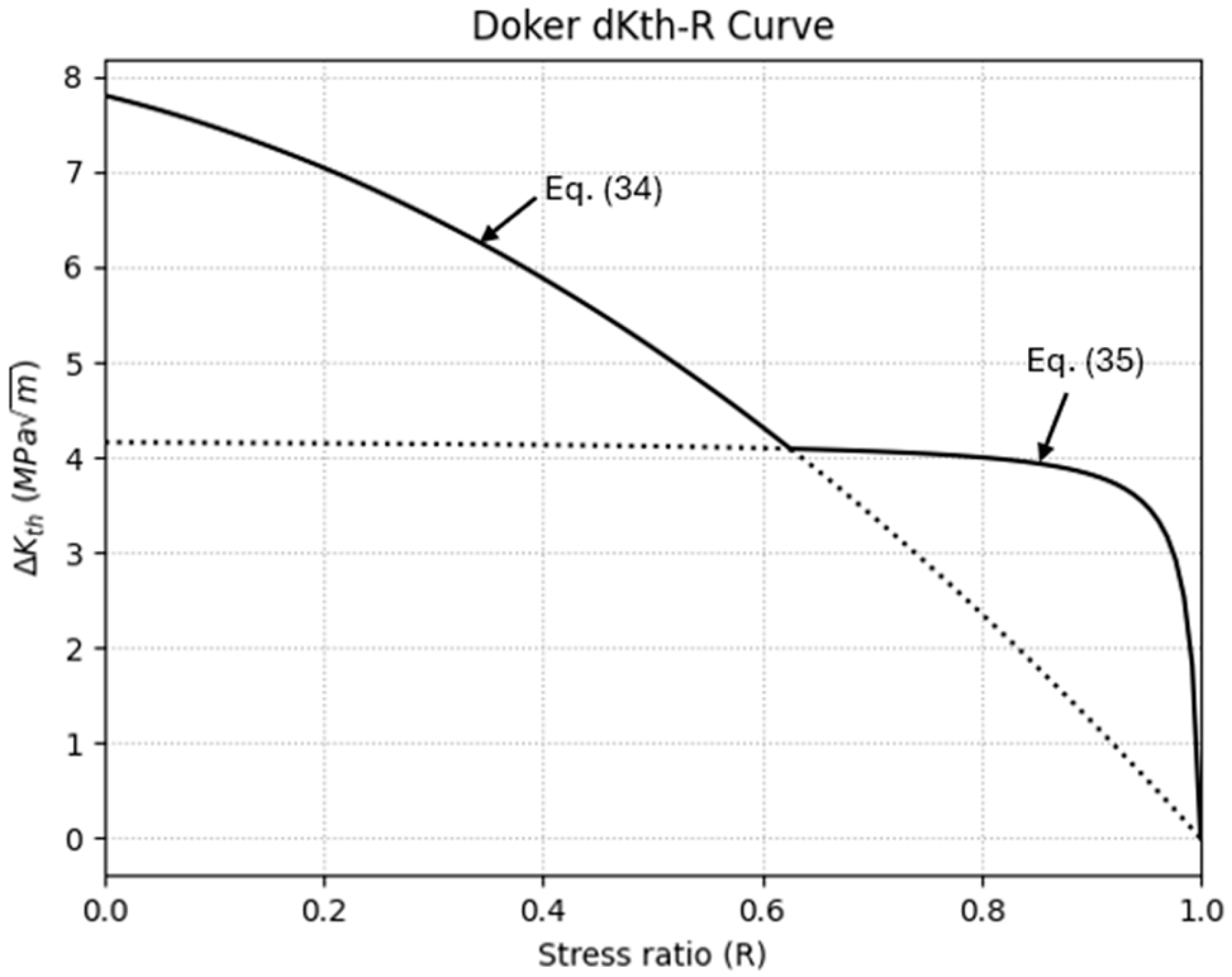
In 1997, Doker [37] proposed a method for threshold determination by plotting ΔKth against the stress ratio R that uses four independent curve-fitting parameters (Kmax,o, ΔKo, αo, βo) obtained from the linear portion of experimental data of CM steels and aluminum alloys. Kmax,o and βo are obtained as the y-intercept and slope, respectively on a Kmax,th-R curve at low R ratios (R < 0.5) and ΔKo and αo are the y-intercept and slope, respectively on a ΔKth-Kmax curve for high stress ratios (R > 0.5). Kmax,th and ΔKth values were obtained from K-decreasing tests following ASTM E647. Solving for ΔKth of these linear regression lines gives two equations:
Δ K t h = ( K m a x , o + β o R ) ( 1 R )   w h e n   R < 0.5
Δ K t h = 1 R 1 R α o Δ K o   w h e n   R > 0.5
These two equations are plotted in Figure 6 for a generic curve that takes into account the observations that ΔKth decreases with increasing R until a critical Rc value (Rc ≈ 0.5–0.6) is reached, where R becomes less influential [10,37].
In 1982, showing microstructural influence, Yoder [51] proposed a cyclic plastic zone-based model to predict ΔKth based on YS and “effective grain size” (ℓ) for α/β titanium alloys like Ti6Al4V; ℓ is the α-lath thickness [52]. Instead of using the ASTM E647 definition of ΔKth, Yoder described it as the “knee” on the da/dN-ΔK curve at the Region I–II transition and physically described it as the point when the size of the plastic zone at the crack tip equals the size of the effective grain size ( r y c ~ l ). The plane strain cyclic plastic zone size can be approximated as
r y c = 1 8 π ( Δ K σ y s ) 2
Similarly, showing microstructural influence, in 2020, ref. [23] proposed a model that directly incorporates microstructural influence and Vickers’ hardness in predicting ΔKth. For Ti6Al4V, the influential microstructural feature is the α-lath thickness. On a log–log scale, ref. [23] showed a negative linear relationship between ΔKth and HV and a positive linear relationship between ΔKth and α-lath thickness, which led to the proposed equation:
Δ K t h = α · l β + ζ · H V δ
where α, β, ζ, and δ are coefficients that depend on R and are fitted to the data, ℓ is the influential microstructural feature (α-lath thickness in µm for Ti6Al4V), and HV is in kgf/mm2. Some drawbacks of this model are that it requires FCG data taken at multiple different stress ratios, there are four curve-fitting parameters, and there is a relatively large error of ±20% with the experimental data. However, it provides a rationale for the material and microstructural influence.

4. FCG Models Applied to EBM Ti6Al4V

4.1. da/dN-ΔK Curve Applied to EBM Ti6Al4V

Some of the above models were originally developed with CM aluminum or steel materials but have recently been applied to AM EBM Ti6Al4V, verifying their potential to be used on this new material to predict FCG behavior and short- and long-crack ΔKth.
Crack closure effects apply to EBM Ti64 [7], showing the same expected relationships as for CM materials: ΔKth decreases with increasing stress ratio, with minimal closure effects at higher stress ratios above R = 0.5. These relationships were true for both horizontal and vertical orientations and between AB and HT cases.
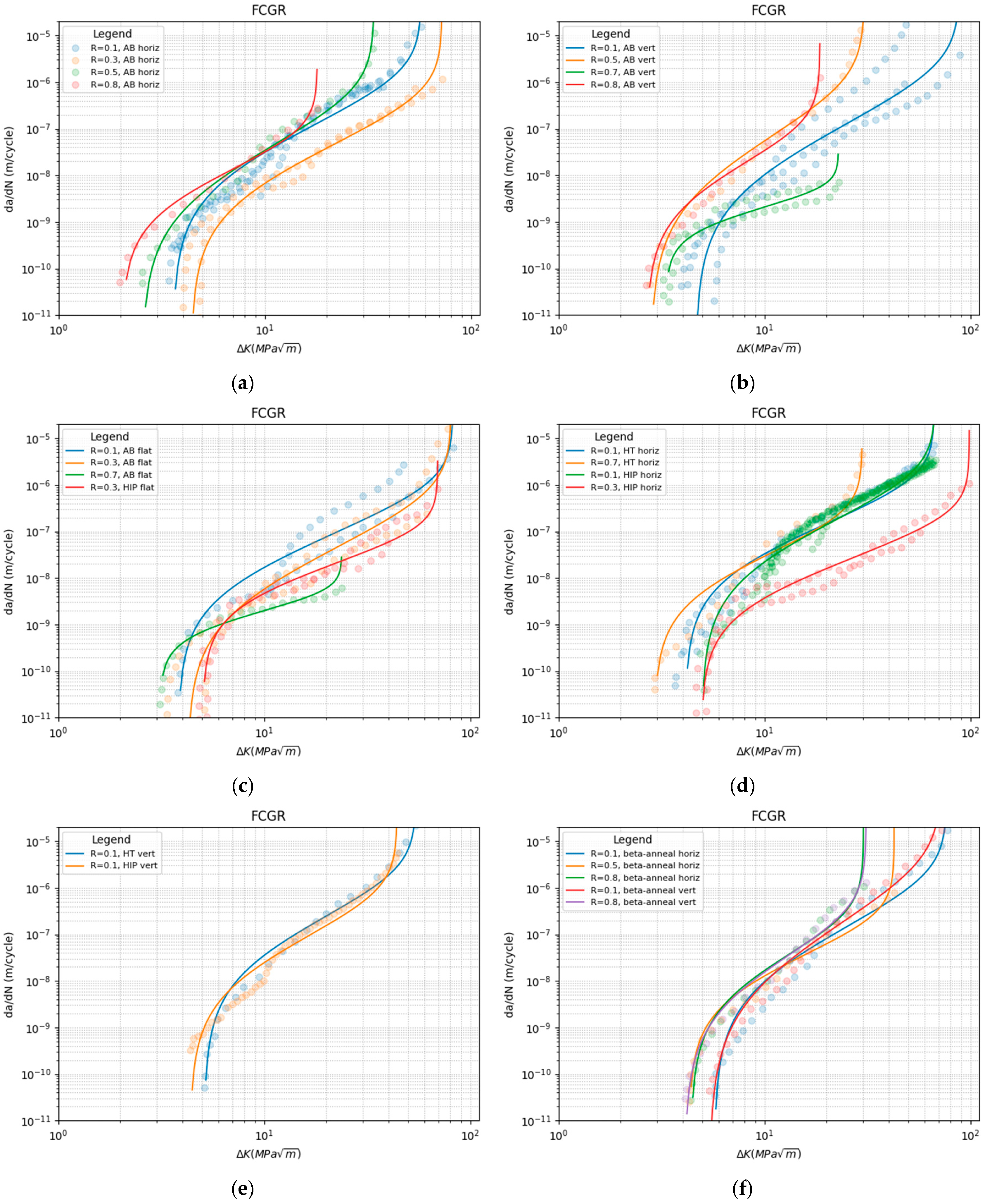
Using the Hartman–Schijve variant Equation (14), when applied to AM Ti6Al4V, ref. [14] found the D and p values to be D = 2.79 × 10⁻¹⁰ and p = 2.12, obtained from curve-fitting with experimental data. Despite the AM process used (EBM, SLM, DMLS, and LENS), different build orientations (horizontal and vertical), and post-processing applied (AB and HIP), the curves fell on the same master curve, with variation coming only from ΔKthr and A. This was also true for 77 other tests on various metals [5,15,16,53,54], implying that the parameters ΔKthr, A, D, and p account for all other factors, including microstructural influences. Using this equation, the contribution of microstructure is unclear [6], although it has been shown through literature that microstructure is influential on material properties, in general, and in the near-threshold region for FCG.
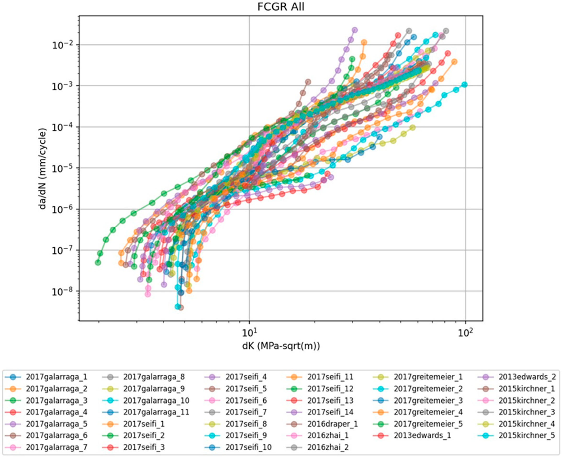
The use of an apparent threshold SIF range ΔKthr allows flexibility for estimating short or long-crack thresholds. A short-crack prediction of ΔKth,SC can be made by setting ΔKthr to an arbitrarily small value (e.g., ΔKth = 0.1 MPa m ) [14]. For long-crack prediction of ΔKth, the use of the Hartman–Schijve variant predicts FCG in Regions I–III and can match empirical data by only adjusting two parameters: ΔKthr and A, given curve-fitting parameters D and p, which are constant for each material. Figure 7 shows experimental data for various stress ratios, orientations, and post-process conditions accumulated from the literature [10,55,56,57,58,59,60].
Using data from the literature, Figure 8 uses the Hartman–Schijve variant Equation (14) to approximate FCG curves by stress ratio, orientation, and post-processing conditions.

4.2. Numerical Simulations Applied to EBM Ti6Al4V

Some researchers have applied PD to the FCG of AM titanium alloys [19,20]. Ref. [19] applied PD to a general AM Ti6Al4V material by simulating both equiaxed and columnar grains. They simulated that coarser grains have greater FCG resistance than finer grains and modeled the deflection angle of cracks as they interact with α-laths at different angles. They showed more deflection when α-laths were perpendicular to the crack growth and less resistance when the α-laths were parallel to the crack growth direction. Ref. [20] used PD to simulate intergranular and transgranular crack growth depending on the size of the grains and validated it with crack length vs. number of cycles (N) curves from literature data in Region II of the FCG curve.
In 2024, ref. [61] proposed a whole rate region model that amends the PD equation to include Regions I–III and simulated FCG curves that aligned with experimental data. Ref. [18] applied XFEM to FCG behavior of AM Ti6Al4V and compared the simulation with laser PBF Ti6Al4V experimental data, with good agreement in Region II. More recently, ref. [62] proposed a multiscale model that uses FEA paired with tensile properties at the crack initiation site and microstructural information to create an FCG model that predicts the S-N curve of AM Ti6Al4V.
More recently, machine learning (ML) has become integrated with AM applications to use high-volume data to optimize build factors like orientation [63]. The authors used ML with AM Ti6Al4V to evaluate the effects of build orientation on microstructure and mechanical behavior, such as surface roughness, dimensional accuracy, and flexural strength. They created contour plots for build angles between 0 and 90° that optimize flexural strength. Although ref. [63] applied ML to mechanical behavior, ML is a growing field, and these concepts can potentially be applied to FCG in the future.

4.3. Predicting ΔKth Applied to EBM Ti6Al4V

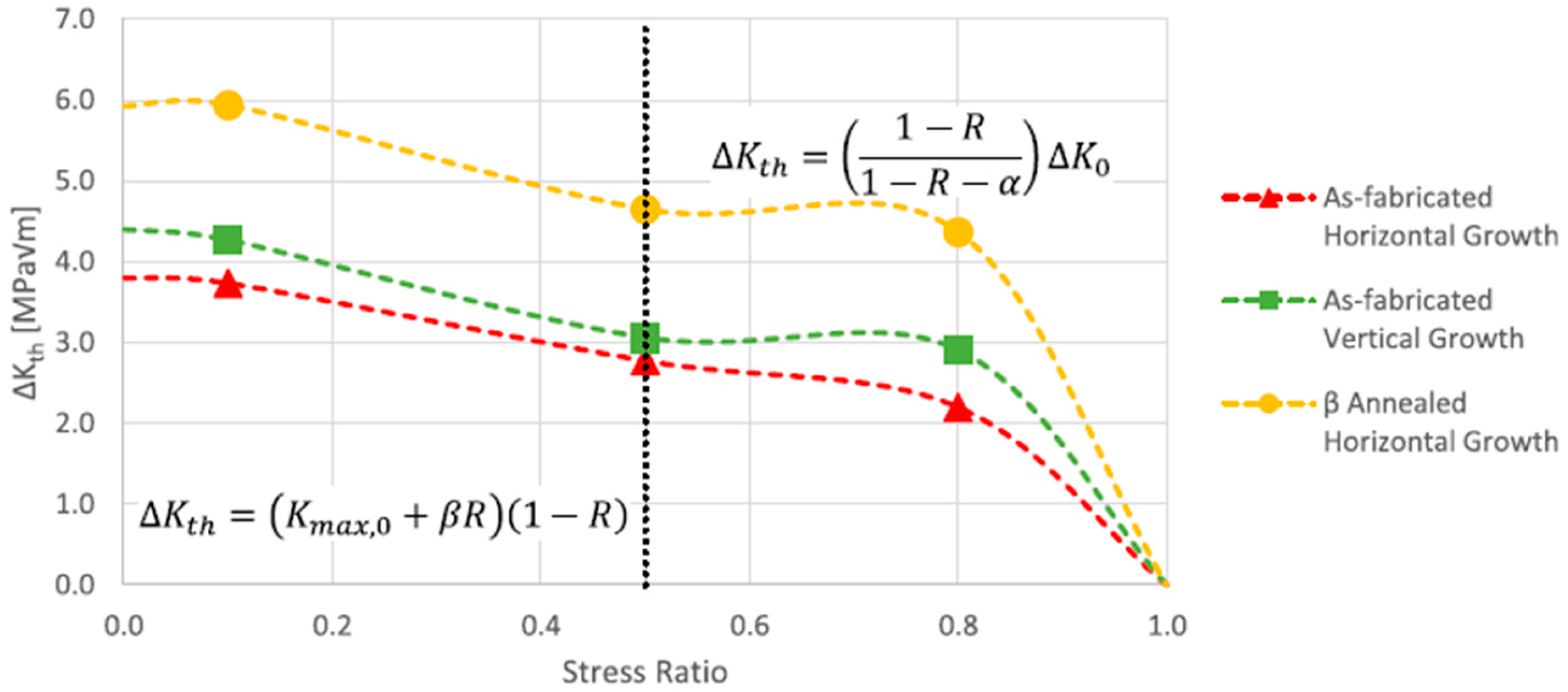
Galarraga [10] applied Doker’s stress ratio curve [37] to relate ΔKth with the stress ratio based on experimental data on EBM Ti6Al4V. They obtained a similar relationship between ΔKth and stress ratio, with a critical Rc = 0.5 for both AB and β-annealed specimens in both the horizontal and vertical orientations. They plotted the curve shown in Figure 9 that follows the same trend as Doker’s [37].
Based on 16 different materials, refs. [21,22] applied Equation (31) to EBM Ti6Al4V to obtain an approximate ideal upper bound σe = 544–605 MPa. Experimental data show a fatigue strength of ~500–600 MPa for the HIP + machined specimen; otherwise, the fatigue limit is much lower than predicted due to the inferior fatigue performance of AM compared to CM (due to high surface roughness and internal defects). This exemplifies the validity of Equation (31) for EBM Ti6Al4V after HIP + machined post-processing.
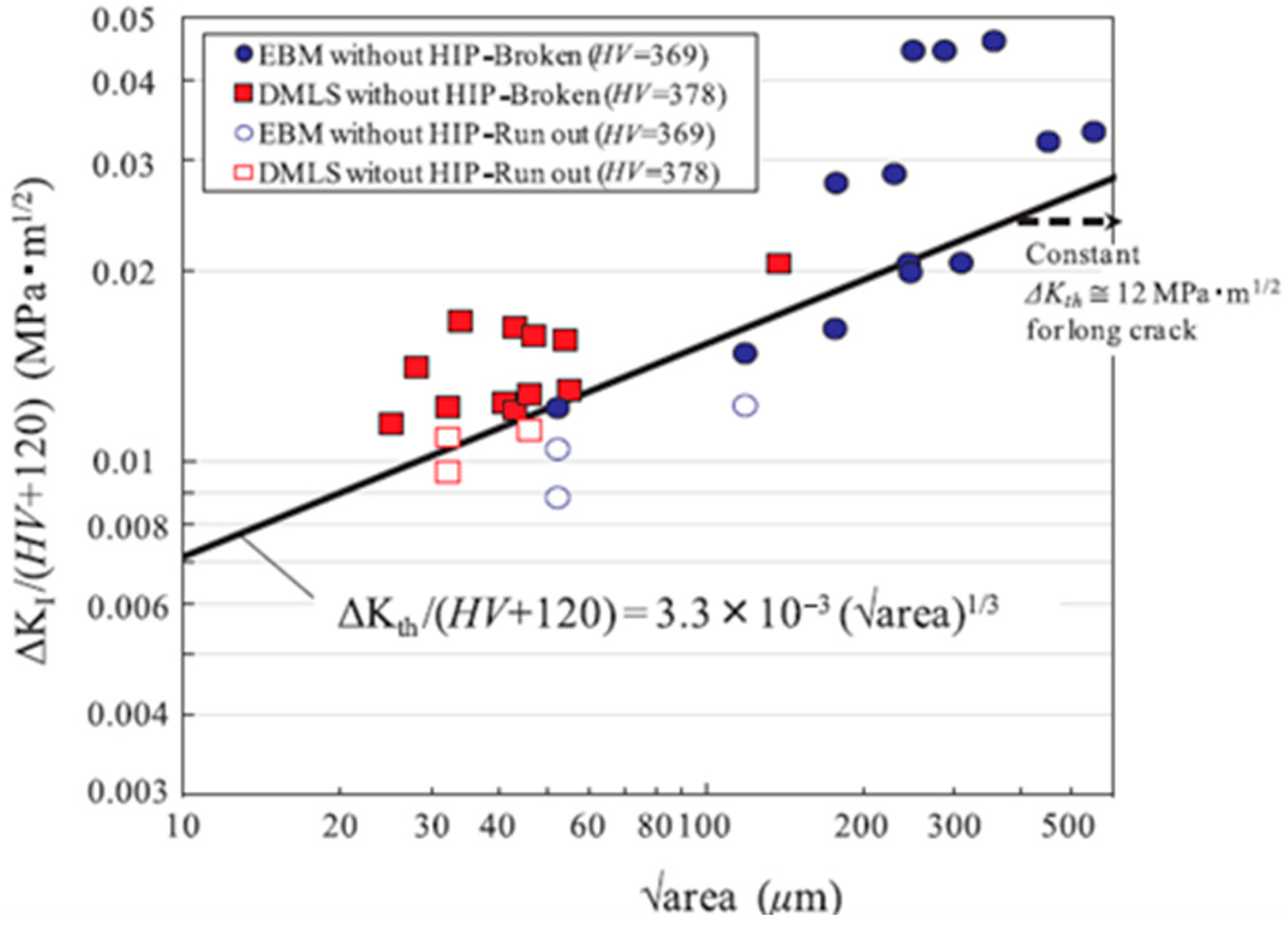
As seen in Figure 10, ref. [21] applied Murakami’s relationship Equation (28) to HIP + machined EBM Ti6Al4V at R = −1 and found the same constants and slope of 1/3 between ΔKth and a r e a on a log–log scale, showing application of Equation (28) on EBM Ti6Al4V. However, they acknowledged that this relationship is conservative for long-crack ΔKth estimation.
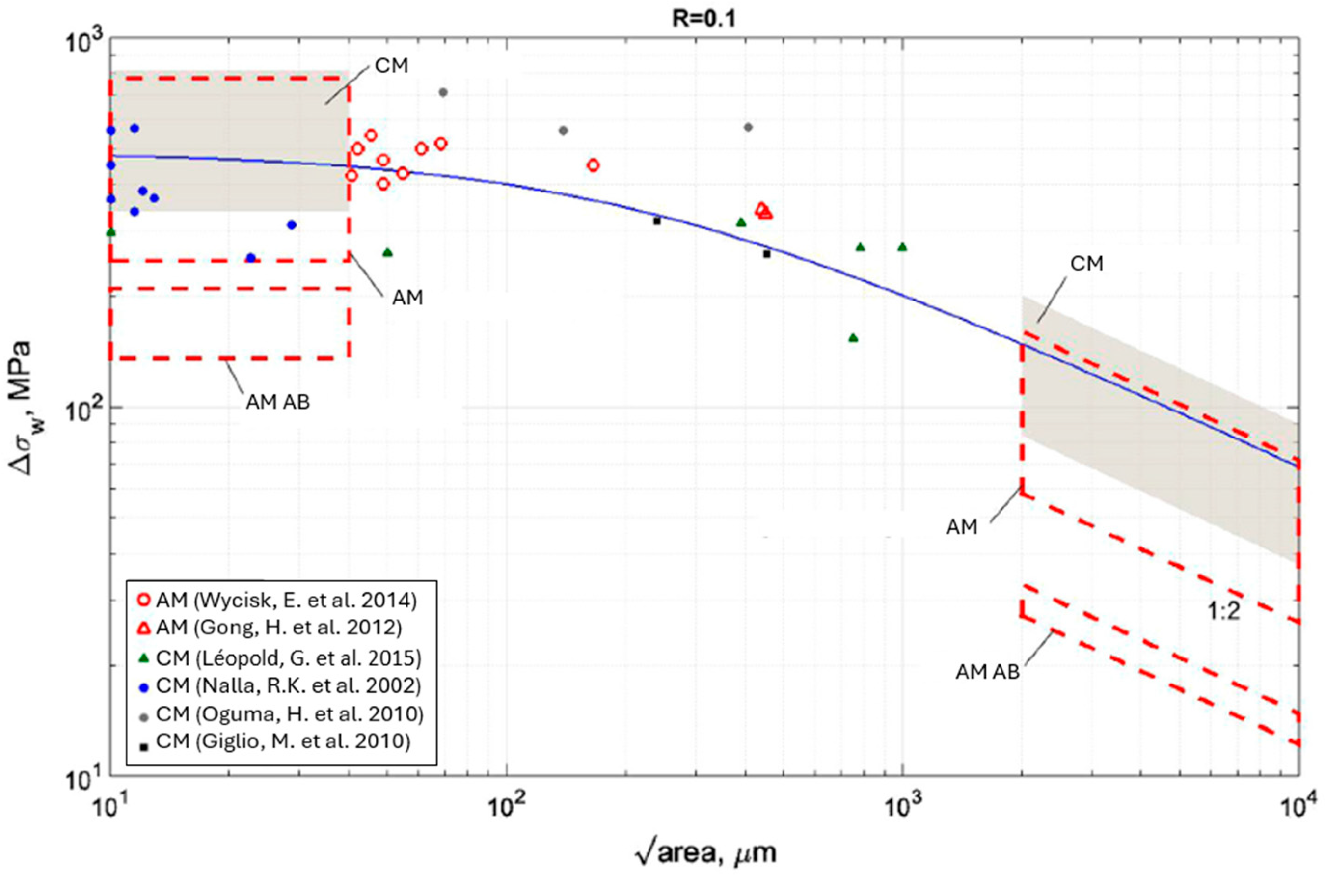
Authors have applied the KT diagram to EBM Ti6Al4V [17,21,22,23,24,26,64,65,66,67,68,69,70,71,72,73,74,75,76,77,78,79,80,81,82,83,84] using El-Haddad’s approximation and Murakami’s method. From these studies, they concluded that these approaches are applicable for approximations of EBM Ti6Al4V. Ref. [26] applied the KT diagram comparing CM Ti6Al4V with AB and post-processed (e.g., heat treated (HT), HIP, and/or machined) AM Ti6Al4V, including EBM, shown in Figure 11. They concluded that small defects are detrimental to fatigue limit and ΔKth in the AB condition. When post-processed, the fatigue limit and ΔKth are comparable to the lower end of CM Ti6Al4V.
However, these authors only applied the KT diagram to specimens that have been machined. It was acknowledged that this method is inaccurate for AB specimens due to the detrimental effects of surface roughness on fatigue strength. Refs. [22,66] recommended treating surface roughness as a long-crack growth problem. Ref. [26] proposed a conversion factor to account for surface roughness effects by measuring a r e a of subsurface pores at a depth of 200 μm:
a r e a = ( p o r e   d e p t h ) · 10
Additionally, refs. [22,47] proposed an evaluation method for equivalent defect size a r e a R :
a r e a R 2 b = 2.97 ( a 2 b ) 3.51 ( a 2 b ) 2 9.74 ( a 2 b ) 3   f o r   a 2 b 0.195
a r e a R 2 b 0.38   f o r   a 2 b 0.195
where the max value of max height Sa is used for a and the mean width of profile RSm is used for 2 b for a 3D roughness profile. a is the vertical distance from root to peak, and 2 b is the horizontal distance from peak to peak.
Other researchers [65] have used the KT diagram to relate d1, ao, and d2 values to microstructural features, showing the dependence of microstructure in the short-crack regime. They found that a o ~ 10 l ; the experimental data was based on CM steels, coppers, and aluminums at R = −1. Refs. [13,23] used the bi-parametric model Equation (37) and used alpha-lath thickness as the microstructural feature to estimate ΔKth = 6.82 MPa m for EBM Ti6Al4V in the AB horizontal condition with a ±10% error with experimental data.

5. Conclusions and Future Directions

In this review, the current state of the literature on FCG models for EBM Ti6Al4V was comprehensively discussed, reviewing both analytical and numerical models for predicting the da/dN-ΔK curve and ΔKth in Region I and simulating FCG behavior.
The literature has shown that the use of many traditional analytical and numerical models is promising for the application to the FCG of EBM Ti6Al4V. Although many experiments have been performed to validate their use, more experimental data are needed to account for the many variables associated with AM, including stress ratio effects, specimen orientation, post-processing, and build height. Additionally, inherent defects and surface roughness present a major challenge to the full adoption of EBM Ti6Al4V in industrial applications. In order to reliably predict FCG for short cracks, these models must be modified to consider these AM-specific factors. More experimental data on short-crack FCG in EBM Ti6Al4V must also be generated to validate these short-crack growth models.
Considering the unique and anisotropic microstructure of EBM Ti6Al4V, a deeper understanding of how the microstructure influences FCG and ΔKth is needed, as well as how crack growth interacts with microstructural features. While the literature has mostly focused on α-lath thickness, there is a need for a complete microstructure–property characterization, including other α and β features and their relationship to FCG in EBM Ti6Al4V.
In light of all these promising developments in analytical and numerical modeling and their application to experimental FCG data for EBM Ti6Al4V, there is still a need for synergy between these models and physical validation through the material microstructure.

Author Contributions

Conceptualization, methodology, software, validation, formal analysis, investigation, resources, data curation, and writing—review and editing, M.R. and N.A.; writing—original draft preparation and visualization, N.A.; supervision, project administration, and funding acquisition, M.R. All authors have read and agreed to the published version of the manuscript.

Funding

This research received no external funding.

Data Availability Statement

No new data were created or analyzed in this study. Data sharing is not applicable to this article.

Acknowledgments

This research was supported by Boeing–Pennell awarded to M. Ramulu. The authors would like to thank the Department of Mechanical Engineering at UW Seattle for the support provided during this study. The authors have reviewed and edited the output and take full responsibility for the content of this publication.

Conflicts of Interest

The authors declare no conflict of interest.

Abbreviations and Nomenclatures

The following abbreviations and nomenclature are used in this manuscript:
ABAs-built
ACRAdjusted compliance ratio
AMAdditive manufacturing
CADComputer aided design
CMConventional manufacturing
CTODCrack tip opening displacement
DMLSDirect metal laser sintering
DTDamage tolerant
EBMElectron beam melting
FCGFatigue crack growth
FEAFinite element analysis
FEMFinite element method
HIPHot isostatic pressing
HTHeat treated
KTKitagawa–Takahashi
LEFMLinear elastic fracture mechanics
LENSLaser-engineered net shaping
NDTNon-destructive testing
PBFPowder bed fusion
PDPeridynamics
R-CurveResistance curve
SIFStress intensity factor
SLMSelective laser melting
SSYSmall-scale yielding
Ti6Al4VTitanium 6–aluminum 4–vanadium alloy
XFEMExtended finite element method
YSYield strength
A Apparent cyclic fracture toughness
a Crack length
a o El-Haddad’s parameter in Equation (20)
a r e a Murakami’s defect size estimation
a r e a c Critical and transition defect size estimation in Equation (32)
a r e a t Critical and transition defect size estimation in Equation (33)
a r e a o Murakami’s initial defect size estimation in Equation (25)
a r e a R Defect size estimation for surface roughness in Equations (39) and (40)
Δ a Crack extension
α ,   β ,   ζ ,   δ Constants in the bi-parametric model Equation (37)
b ( x , t ) External body forces in peridynamics Equation (16)
C , m Constants in Paris Equation (3)
γ Constant in Walker Equation (11)
d 1 Length of microcrack threshold
d 2 Length of long-crack threshold
D , p Constants in Hartman–Schijve variant Equation (14)
d a / d N Crack length per cycle
ε c o r e Bond strain in peridynamics Equation (16)
f Newman’s crack closure factor Equation (10)
H x All nearby points within a horizon in the peridynamics Equation (16)
H V Vicker’s hardness
K c Fracture toughness
K m i n Minimum applied SIF
K m a x Maximum applied SIF
K o p SIF when a crack first opens
K m a x , o , Δ K o , α o , β o Constants in Doker’s Stress Ratio Equations (34) and (35)
Δ K SIF range
Δ K c Overload SIF range
Δ K e f f Effective SIF range
Δ K t h Threshold SIF range (for long cracks)
Δ K t h , S C Threshold SIF range (for short cracks)
Δ K t h , e f f Intrinsic threshold SIF range
Δ K t h , o p Extrinsic threshold SIF range
Δ K t h r Apparent threshold SIF range
Δ κ Schwalbe factor Equation (13)
l Microstructural feature (μm)
λ , B Constants in peridynamics Equation (16)
p ( x ) Mass density of point x in peridynamics Equation (16)
R Stress ratio
r , q Constants in NASGRO Equation (15)
r y c Cyclic plastic zone
σ m i n Minimum applied stress
σ m a x Maximum applied stress
Δ σ Stress range
Δ σ e “Defect-free” fatigue strength
Δ σ t h Fatigue strength
σ y s Yield strength
t Time in peridynamics Equation (16)
U Elber’s crack closure ratio Equation (8)
u ( x , t ) Displacement of material at point x and time t in peridynamics Equation (16)
u ¨ ( x , t ) Acceleration of material at point x and time t in peridynamics Equation (16)
x Position of a point in peridynamics Equation (16)
x Position of a neighboring point in peridynamics Equation (16)
Y Geometry correction factor

References

  1. Kundu, S.; Jones, R.; Peng, D.; Matthews, N.; Alankar, A.; Raman, S.R.K.; Huang, P. Review of Requirements for the Durability and Damage Tolerance Certification of Additively Manufactured Aircraft Structural Parts and AM Repairs. Materials 2020, 13, 1341. [Google Scholar] [CrossRef] [PubMed]
  2. Findlay, S.J.; Harrison, N.D. Why Aircraft Fail. Mater. Today 2002, 5, 18–25. [Google Scholar] [CrossRef]
  3. ASTM E647-15e1; Standard Test Method for Measurement of Fatigue Crack Growth Rates. ASTM International: West Conshohocken, PA, USA, 2015. [CrossRef]
  4. Maierhofer, J.; Gänser, H.-P.; Pippan, R. Modified Kitagawa–Takahashi Diagram Accounting for Finite Notch Depths. Int. J. Fatigue 2015, 70, 503–509. [Google Scholar] [CrossRef]
  5. Jones, R.; Michopoulos, J.G.; Iliopoulos, A.P.; Singh Raman, R.K.; Phan, N.; Nguyen, T. Representing Crack Growth in Additively Manufactured Ti-6Al-4V. Int. J. Fatigue 2018, 116, 610–622. [Google Scholar] [CrossRef]
  6. Jones, R.; Singh Raman, R.K.; McMillan, A.J. Crack Growth: Does Microstructure Play a Role? Eng. Fract. Mech. 2018, 187, 190–210. [Google Scholar] [CrossRef]
  7. Zerbst, U.; Vormwald, M.; Pippan, R.; Gänser, H.-P.; Sarrazin-Baudoux, C.; Madia, M. About the Fatigue Crack Propagation Threshold of Metals as a Design Criterion—A Review. Eng. Fract. Mech. 2016, 153, 190–243. [Google Scholar] [CrossRef]
  8. Revankar, S.; Wolf, B.; Roznic, J. Metal Fatigue Crack Growth Models. Int. J. Adv. Eng. Appl. 2012, 5, 85–91. [Google Scholar]
  9. Zerbst, U.; Bruno, G.; Buffière, J.-Y.; Wegener, T.; Niendorf, T.; Wu, T.; Zhang, X.; Kashaev, N.; Meneghetti, G.; Hrabe, N.; et al. Damage Tolerant Design of Additively Manufactured Metallic Components Subjected to Cyclic Loading: State of the Art and Challenges. Prog. Mater. Sci. 2021, 121, 100786. [Google Scholar] [CrossRef]
  10. Galarraga, H.; Warren, R.J.; Lados, D.A.; Dehoff, R.R.; Kirka, M.M. Fatigue Crack Growth Mechanisms at the Microstructure Scale in As-Fabricated and Heat Treated Ti-6Al-4V ELI Manufactured by Electron Beam Melting (EBM). Eng. Fract. Mech. 2017, 176, 263–280. [Google Scholar] [CrossRef]
  11. Oberwinkler, B. Modeling the Fatigue Crack Growth Behavior of Ti-6Al-4V by Considering Grain Size and Stress Ratio. Mater. Sci. Eng. A 2011, 528, 5983–5992. [Google Scholar] [CrossRef]
  12. Wycisk, E.; Solbach, A.; Siddique, S.; Herzog, D.; Walther, F.; Emmelmann, C. Effects of Defects in Laser Additive Manufactured Ti-6Al-4V on Fatigue Properties. Phys. Procedia 2014, 56, 371–378. [Google Scholar] [CrossRef]
  13. Rigon, D.; Meneghetti, G. An Engineering Approach to Estimate Fatigue Thresholds of Wrought and Additively Manufactured Defective Metallic Materials. Procedia Struct. Integr. 2021, 34, 154–159. [Google Scholar] [CrossRef]
  14. Iliopoulos, A.P.; Jones, R.; Michopoulos, J.G.; Phan, N.; Rans, C. Further Studies into Crack Growth in Additively Manufactured Materials. Materials 2020, 13, 2223. [Google Scholar] [CrossRef]
  15. Jones, R.; Rans, C.; Iliopoulos, A.P.; Michopoulos, J.G.; Phan, N.; Peng, D. Modelling the Variability and the Anisotropic Behaviour of Crack Growth in SLM Ti-6Al-4V. Materials 2021, 14, 1400. [Google Scholar] [CrossRef] [PubMed]
  16. Iliopoulos, A.; Jones, R.; Michopoulos, J.; Phan, N.; Singh Raman, R.K. Crack Growth in a Range of Additively Manufactured Aerospace Structural Materials. Aerospace 2018, 5, 118. [Google Scholar] [CrossRef]
  17. Madia, M.; Zerbst, U.; Werner, T. Estimation of the Kitagawa-Takahashi Diagram by Cyclic R Curve Analysis. Procedia Struct. Integr. 2022, 38, 309–316. [Google Scholar] [CrossRef]
  18. Verma, R.; Kumar, P.; Jayaganthan, R.; Pathak, H. Extended Finite Element Simulation on Tensile, Fracture Toughness and Fatigue Crack Growth Behaviour of Additively Manufactured Ti6Al4V Alloy. Theor. Appl. Fract. Mech. 2022, 117, 103163. [Google Scholar] [CrossRef]
  19. Liu, B.; Wang, K.; Bao, R.; Sui, F. The Effects of α/β Phase Interfaces on Fatigue Crack Deflections in Additively Manufactured Titanium Alloy: A Peridynamic Study. Int. J. Fatigue 2020, 137, 105622. [Google Scholar] [CrossRef]
  20. Karpenko, O.; Oterkus, S.; Oterkus, E. Peridynamic Analysis to Investigate the Influence of Microstructure and Porosity on Fatigue Crack Propagation in Additively Manufactured Ti6Al4V. Eng. Fract. Mech. 2022, 261, 108212. [Google Scholar] [CrossRef]
  21. Masuo, H.; Tanaka, Y.; Morokoshi, S.; Yagura, H.; Uchida, T.; Yamamoto, Y.; Murakami, Y. Influence of Defects, Surface Roughness and HIP on the Fatigue Strength of Ti-6Al-4V Manufactured by Additive Manufacturing. Int. J. Fatigue 2018, 117, 163–179. [Google Scholar] [CrossRef]
  22. Nakatani, M.; Masuo, H.; Tanaka, Y.; Murakami, Y. Effect of Surface Roughness on Fatigue Strength of Ti-6Al-4V Alloy Manufactured by Additive Manufacturing. Procedia Struct. Integr. 2019, 19, 294–301. [Google Scholar] [CrossRef]
  23. Rigon, D.; Meneghetti, G. An Engineering Estimation of Fatigue Thresholds from a Microstructural Size and Vickers Hardness: Application to Wrought and Additively Manufactured Metals. Int. J. Fatigue 2020, 139, 105796. [Google Scholar] [CrossRef]
  24. Persenot, T.; Burr, A.; Martin, G.; Buffiere, J.-Y.; Dendievel, R.; Maire, E. Effect of Build Orientation on the Fatigue Properties of As-Built Electron Beam Melted Ti-6Al-4V Alloy. Int. J. Fatigue 2019, 118, 65–76. [Google Scholar] [CrossRef]
  25. Rigon, D.; Meneghetti, G. Estimating the Fatigue Thresholds of Additively Manufactured Metallic Materials with Consideration of Defects. Procedia Struct. Integr. 2022, 38, 70–76. [Google Scholar] [CrossRef]
  26. Beretta, S.; Romano, S. A Comparison of Fatigue Strength Sensitivity to Defects for Materials Manufactured by AM or Traditional Processes. Int. J. Fatigue 2017, 94, 178–191. [Google Scholar] [CrossRef]
  27. Galarraga, H.; Lados, D.A.; Dehoff, R.R.; Kirka, M.M.; Nandwana, P. Effects of the Microstructure and Porosity on Properties of Ti-6Al-4V ELI Alloy Fabricated by Electron Beam Melting (EBM). Addit. Manuf. 2016, 10, 47–57. [Google Scholar] [CrossRef]
  28. Paris, P.; Erdogan, F. A Critical Analysis of Crack Propagation Laws. J. Basic. Eng. 1963, 85, 528–533. [Google Scholar] [CrossRef]
  29. Forman, R.G.; Kearney, V.E.; Engle, R.M. Numerical Analysis of Crack Propagation in Cyclic-Loaded Structures. J. Basic. Eng. 1967, 89, 459–463. [Google Scholar] [CrossRef]
  30. Wolf, E. Fatigue Crack Closure under Cyclic Tension. Eng. Fract. Mech. 1970, 2, 37–45. [Google Scholar] [CrossRef]
  31. Walker, K. The Effect of Load Ratio During Crack Propagation and Fatigue for 2024T3 and 7075-T6 Aluminum; ASTM Selected Technical Papers; ASTM International: West Conshohocken, PA, USA, 1970; Volume STP462, pp. 1–14. [Google Scholar] [CrossRef]
  32. Hartman, A.; Schijve, J. The Effects of Environment and Load Frequency on the Crack Propagation Law for Macro Fatigue Crack Growth in Aluminium Alloys. Eng. Fract. Mech. 1970, 1, 615–631. [Google Scholar] [CrossRef]
  33. Klesnil, M.; Lukáš, P. Influence of Strength and Stress History on Growth and Stabilisation of Fatigue Cracks. Eng. Fract. Mech. 1972, 4, 77–92. [Google Scholar] [CrossRef]
  34. Jones, R. Fatigue Crack Growth and Damage Tolerance. Fatigue Fract. Eng. Mater. Struct. 2014, 37, 463–483. [Google Scholar] [CrossRef]
  35. Tanaka, K.; Akiniwa, Y. Resistance-Curve Method for Predicting Propagation Threshold of Short Fatigue Cracks at Notches. Eng. Fract. Mech. 1988, 30, 863–876. [Google Scholar] [CrossRef]
  36. Huang, X.; Moan, T. Improved Modeling of the Effect of R-Ratio on Crack Growth Rate. Int. J. Fatigue 2007, 29, 591–602. [Google Scholar] [CrossRef]
  37. Doker, H. Fatigue Crack Growth Threshold: Implications, Determination and Data Evaluation. Int. J. Fatigue 1997, 19, 145–149. [Google Scholar] [CrossRef]
  38. Newman, J.C., Jr. FASTRAN-2: A Fatigue Crack Growth Structural Analysis Program; NASA STI/Recon Technical Report N NASA TM-104159; NASA Tech Briefs: New York, NY, USA, 1992. [Google Scholar]
  39. Schwalbe, K.-H. On the Beauty of Analytical Models for Fatigue Crack Propagation and Fracture—A Personal Historical Review. J. ASTM Int. 2010, 7, 1–53. [Google Scholar] [CrossRef]
  40. Moes, N.; Dolbow, J.; Belytschko, T. A Finite Element Method for Crack Growth without Remeshing. Int. J. Numer. Methods Eng. 1999, 46, 131–150. [Google Scholar] [CrossRef]
  41. Antunes, F.V.; Branco, R.; Prates, P.A.; Borrego, L. Fatigue Crack Growth Modelling Based on CTOD for the 7050-T6 Alloy. Fatigue Fract. Eng. Mater. Struct. 2017, 40, 1309–1320. [Google Scholar] [CrossRef]
  42. Marques, B.; Borges, M.F.; Antunes, F.V.; Vasco-Olmo, J.M.; Díaz, F.A.; James, M.N. Limitations of Small-Scale Yielding for Fatigue Crack Growth. Eng. Fract. Mech. 2021, 252, 107806. [Google Scholar] [CrossRef]
  43. Silling, S.A. Reformulation of Elasticity Theory for Discontinuities and Long-Range Forces. J. Mech. Phys. Solids 2000, 48, 175–209. [Google Scholar] [CrossRef]
  44. Silling, S.A.; Lehoucq, R.B. Peridynamic Theory of Solid Mechanics. Adv. Appl. Mech. 2010, 44, 73–168. [Google Scholar] [CrossRef]
  45. Silling, S.; Askari, A. Peridynamic Model for Fatigue Cracking; Technical Report; Sandia National Laboratories (SNL-NM): Albuquerque, NM, USA, 2014. [Google Scholar]
  46. Haddad, M.H.E.; Topper, T.H.; Smith, K.N. Prediction of Non Propagating Cracks. Eng. Fract. Mech. 1979, 11, 573–584. [Google Scholar] [CrossRef]
  47. Murakami, Y. Metal Fatigue: Effects of Small Defects and Nonmetallic Inclusions; Elsevier: Amsterdam, The Netherlands, 2002; ISBN 978-0-08-044064-4. [Google Scholar]
  48. Kitagawa, H. Applicability of Fracture Mechanics to Very Small Cracks or the Cracks in the Early Stage. In Proceedings of the Second International Conference on Mechanical Behavior of Materials, Boston, MA, USA, 16–20 August 1976; pp. 627–631. [Google Scholar]
  49. Akiniwa, Y.; Zhang, L.M.; Tanaka, K. Prediction of The Fatigue Limit of Cracked Specimens Based on the Cyclic R-Curve Method. Fatigue Fract. Eng. Mater. Struct. 1997, 20, 1387–1398. [Google Scholar] [CrossRef]
  50. Murakami, Y.; Masahiro, E. Quantitative Evaluation of Fatigue Strength of Metals Containing Various Small Defects or Cracks. Eng. Fract. Mech. 1983, 17, 1–15. [Google Scholar] [CrossRef]
  51. Yoder, G.R.; Cooley, L.A.; Crooker, T.W. On Microstructural Control of Near-Threshold Fatigue Crack Growth in 7000-Series Aluminum Alloys. Scr. Metall. 1982, 16, 1021–1025. [Google Scholar] [CrossRef]
  52. Herold, H.; Streitenberger, M.; Zinke, M.; Orazi, L.; Cammarota, G.P. An Experimental and Theoretical Approach for an Estimation of ΔKth. Fatigue Fract. Eng. Mater. Struct. 2000, 23, 805–812. [Google Scholar] [CrossRef]
  53. Jones, R.; Kovarik, O.; Cizek, J.; Ang, A.; Lang, J. Crack Growth in Conventionally Manufactured Pure Nickel, Titanium and Aluminum and the Cold Spray Addively Manufactured Equivalents. Addit. Manuf. Lett. 2022, 3, 100043. [Google Scholar] [CrossRef]
  54. Jones, R.; Cizek, J.; Kovarik, O.; Lang, J.; Ang, A.; Michopoulos, J.G. Describing Crack Growth in Additively Manufactured Scalmalloy. Addit. Manuf. Lett. 2021, 1, 100020. [Google Scholar] [CrossRef]
  55. Seifi, M.; Salem, A.; Satko, D.; Shaffer, J.; Lewandowski, J.J. Defect Distribution and Microstructure Heterogeneity Effects on Fracture Resistance and Fatigue Behavior of EBM Ti–6Al–4V. Int. J. Fatigue 2017, 94, 263–287. [Google Scholar] [CrossRef]
  56. Draper, S.; Lerch, B.; Rogers, R.; Martin, R.; Locci, I.; Garg, A. Materials Characterization of Electron Beam Melted Ti-6Al-4V. In Proceedings of the 13th World Conference on Titanium, San Diego, CA, USA, 16–20 August 2015; Venkatesh, V., Pilchak, A.L., Allison, J.E., Ankem, S., Boyer, R., Christodoulou, J., Fraser, H.L., Imam, M.A., Kosaka, Y., Rack, H.J., et al., Eds.; John Wiley and Sons: Hoboken, NJ, USA, 2016; pp. 1433–1440. ISBN 978-1-119-28326-3. [Google Scholar]
  57. Zhai, Y.; Galarraga, H.; Lados, D.A. Microstructure, Static Properties, and Fatigue Crack Growth Mechanisms in Ti-6Al-4V Fabricated by Additive Manufacturing: LENS and EBM. Eng. Fail. Anal. 2016, 69, 3–14. [Google Scholar] [CrossRef]
  58. Greitemeier, D.; Palm, F.; Syassen, F.; Melz, T. Fatigue Performance of Additive Manufactured TiAl6V4 Using Electron and Laser Beam Melting. Int. J. Fatigue 2017, 94, 211–217. [Google Scholar] [CrossRef]
  59. Edwards, P.; O’Conner, A.; Ramulu, M. Electron Beam Additive Manufacturing of Titanium Components: Properties and Performance. J. Manuf. Sci. Eng. 2013, 135, 061016. [Google Scholar] [CrossRef]
  60. Kirchner, A.; Klöden, B.; Weißgärber, T.; Kieback, B.; Schoberth, A.; Bagehorn, S.; Greitemeier, D. Mechanical Properties of Ti-6Al-4V Additively Manufactured by Electron Beam Melting. In Proceedings of the European Powder Metallurgy Association 2015 Congress & Exhibition, Reims, France, 4–7 October 2015. [Google Scholar]
  61. Zhang, H.; Yao, L.; Zheng, X.; Zhou, J. A Whole-Rate-Region Fatigue Crack Growth Model Incorporating Nonlinear Rate Evolution Characteristics Based on a Peridynamic Approach. J. Eng. Mech. 2024, 150, 04024094. [Google Scholar] [CrossRef]
  62. Chi, W.; Wang, W.; Zhou, H.; Yan, R.; Mikami, Y. Multiscale Modelling of Additively Manufactured Ti-6Al-4V Alloy: Fatigue Performance Evaluation from Material to Structural Level. Int. J. Fatigue 2025, 201, 109181. [Google Scholar] [CrossRef]
  63. Sicakdemir, B.; Özsoy, K. Machine Learning and Optimization-Driven Analysis of Build Orientation Effects on the Microstructure and Mechanical Behavior of Ti-6al-4v Fabricated by Electron Beam Melting Additive Manufacturing. J. Mater. Eng. Perform. 2026, 1–19. [Google Scholar] [CrossRef]
  64. Bergant, M.A.; Soria, S.R.; Bustos, R.I.; Soul, H.R.; Yawny, A.A. On the Relative Significance of Roughness, Printing Defects and Microstructure on the Fatigue Behavior of Electron Beam Melted Ti-6Al-4V. Fatigue Fract. Eng. Mater. Struct. 2025, 48, 1647–1666. [Google Scholar] [CrossRef]
  65. Chandran, K.S.R. The Finding of the Reciprocal Relationship between Fatigue (S-N) Behavior and Fatigue Crack Growth Behavior Enabling Interconversion of Data in Structural Materials. Materialia 2022, 25, 101541. [Google Scholar] [CrossRef]
  66. Macallister, N.; Becker, T.H. Fatigue Life Estimation of Additively Manufactured Ti-6Al-4V: Sensitivity, Scatter and Defect Description in Damage-Tolerant Models. Acta Mater. 2022, 237, 118189. [Google Scholar] [CrossRef]
  67. Nalla, R.K.; Boyce, B.L.; Campbell, J.P.; Peters, J.O.; Ritchie, R.O. Influence of Microstructure on High-Cycle Fatigue of Ti-6Al-4V: Bimodal vs. Lamellar Structures. Metall. Mater. Trans. A 2002, 33, 899–918. [Google Scholar] [CrossRef]
  68. Rafi, H.K.; Karthik, N.V.; Gong, H.; Starr, T.L.; Stucker, B.E. Microstructures and Mechanical Properties of Ti6Al4V Parts Fabricated by Selective Laser Melting and Electron Beam Melting. J. Mater. Eng. Perform. 2013, 22, 3872–3883. [Google Scholar] [CrossRef]
  69. Leuders, S.; Thöne, M.; Riemer, A.; Niendorf, T.; Tröster, T.; Richard, H.A.; Maier, H.J. On the Mechanical Behaviour of Titanium Alloy TiAl6V4 Manufactured by Selective Laser Melting: Fatigue Resistance and Crack Growth Performance. Int. J. Fatigue 2013, 48, 300–307. [Google Scholar] [CrossRef]
  70. Gong, H.; Rafi, K.; Starr, T.; Stucker, B. Effect of Defects on Fatigue Tests of As-Built Ti-6al-4v Parts Fabricated by Selective Laser Melting. In Proceedings of the 23th Annual International Solid Freeform Fabrication Symposium, Austin, TX, USA, 6–8 August 2012; pp. 499–506. [Google Scholar]
  71. Oguma, H.; Nakamura, T. The Effect of Microstructure on Very High Cycle Fatigue Properties in Ti–6Al–4V. Scr. Mater. 2010, 63, 32–34. [Google Scholar] [CrossRef]
  72. Léopold, G.; Nadot, Y.; Billaudeau, T.; Mendez, J. Influence of Artificial and Casting Defects on Fatigue Strength of Moulded Components in Ti-6Al-4V Alloy. Fatigue Fract. Eng. Mater. Struct. 2015, 38, 1026–1041. [Google Scholar] [CrossRef]
  73. Giglio, M.; Beretta, S.; Mariani, U.; Ratti, G. Defect Tolerance Assessment of a Helicopter Component Subjected to Multiaxial Load. Eng. Fract. Mech. 2010, 77, 2479–2490. [Google Scholar] [CrossRef]
  74. Bagehorn, S.; Mertens, T.; Greitemeier, D.; Carton, L.; Schoberth, A. Surface FInishing of Additive Manufactured Ti-6Al-4V—A Comparison of Electrochemical and Mechanical Treatments. In Proceedings of the 6th European Conference for Aeronautics and Space Sciences, Kraków, Poland, 29 June–3 July 2015. [Google Scholar]
  75. Baufeld, B.; Brandl, E.; Van Der Biest, O. Wire Based Additive Layer Manufacturing: Comparison of Microstructure and Mechanical Properties of Ti–6Al–4V Components Fabricated by Laser-Beam Deposition and Shaped Metal Deposition. J. Mater. Process. Technol. 2011, 211, 1146–1158. [Google Scholar] [CrossRef]
  76. Grylls, R. LENS Process White Paper: Fatigue Testing of LENS Ti-6-4; Technical Brief; OPTOMEC: Albuquerque, NM, USA, 2005. [Google Scholar]
  77. Greitemeier, D.; Dalle Donne, C.; Schoberth, A.; Jurgens, M.; Eufinger, J.; Melz, T. Microstructure and Mechanical Properties. Appl. Mech. Mater. 2015, 807, 169–180. [Google Scholar] [CrossRef]
  78. Wycisk, E.; Emmelmann, C.; Siddique, S.; Walther, F. High Cycle Fatigue (HCF) Performance of Ti-6Al-4V Alloy Processed by Selective Laser Melting. Adv. Mater. Res. 2013, 816–817, 134–139. [Google Scholar] [CrossRef]
  79. Department of Defense Military Handbook. Titanium and Titanium Alloys; Department of Defense Military: Washington, VA, USA, 1974. [Google Scholar]
  80. Niinomi, M. Mechanical Properties of Biomedical Titanium Alloys. Mater. Sci. Eng. A 1998, 243, 231–236. [Google Scholar] [CrossRef]
  81. Morrissey, R.; Nicholas, T. Staircase Testing of a Titanium Alloy in the Gigacycle Regime. Int. J. Fatigue 2006, 28, 1577–1582. [Google Scholar] [CrossRef]
  82. Nakamura, T.; Oguma, H.; Shinohara, Y. The Effect of Vacuum-like Environment inside Sub-Surface Fatigue Crack on the Formation of ODA Fracture Surface in High Strength Steel. Procedia Eng. 2010, 2, 2121–2129. [Google Scholar] [CrossRef]
  83. Oberwinkler, B.; Riedler, M.; Eichlseder, W. Importance of Local Microstructure for Damage Tolerant Light Weight Design of Ti–6Al–4V Forgings. Int. J. Fatigue 2010, 32, 808–814. [Google Scholar] [CrossRef]
  84. Oberwinkler, B.; Redik, S.; Leitner, H. Analysis of Short Crack Growth for Two Representative Light Metals. In Proceedings of the 12th International Conference on Fracture, Ottawa, ON, Canada, 12–17 July 2009; pp. 1–9. [Google Scholar]
Figure 1. Schematic of the EBM build chamber.
Metals 16 00440 g001
Figure 2. da/dN-ΔK FCG curve composed of Regions I, II, and III.
Metals 16 00440 g002
Figure 3. Kitagawa–Takahashi (KT) diagram intersects at crack depth ao, with the El-Haddad approximation dividing microcracks (blue), physically short cracks (green), and long cracks (red). Reprinted with permission from [17].
Metals 16 00440 g003
Figure 4. Cyclic R-curve (a) and the buildup of crack closure as plasticity-induced (red) and roughness- and oxide-induced (blue) (b). Reprinted with permission from [17].
Metals 16 00440 g004
Figure 6. Doker’s stress ratio curve, where Equations (34) and (35) intersect at R > 0.5–0.6.
Metals 16 00440 g006
Figure 7. FCG experimental data of EBM Ti6Al4V for a variety of stress ratios, orientations, and post-process conditions, where each color is a different dataset [10,55,56,57,58,59,60].
Metals 16 00440 g007
Figure 8. The The Hartman–Schijve variant equation applied to experimental data at different stress ratios for AB horiz specimen (a), AB vert specimen (b), AB and HIP flat specimen (c), HT and HIP horiz specimen (d), HT and HIP vert specimen (e), and β-annealed horiz and vert specimen (f) [10,55,56,57,58,59,60].
Metals 16 00440 g008
Figure 9. Doker’s stress ratio curve applied to EBM Ti6Al4V, with Equation (34) applied at R < 0.5 and Equation (35) applied to R > 0.5. Reprinted with permission from [10].
Metals 16 00440 g009
Figure 10. Predicting ΔKth based on HV from AM metals. Reprinted with permission from [21].
Metals 16 00440 g010
Figure 11. KT diagram comparing CM Ti6Al4V to AM Ti6Al4V [12,17,21,22,23,24,26,64,65,66,67,68,69,70,71,72,73,74,75,76,77,78,79,80,81,82,83,84], where the brown squares represent CM and the red dashed boxes represent AM. Adapted with permission from [26].
Metals 16 00440 g011
Table 1. FCG models that predict the da/dN-ΔK curve and the region they apply to.
ModelEquationRegion
1963: Paris Law [28] d a d N = C ( Δ K ) m II
1967: Forman [29] d a d N = C ( Δ K ) m ( 1 R ) K c Δ K II–III
1970: Elber [30] d a d N = C ( Δ K e f f ) m = C ( U Δ K ) m I
1970: Walker [31] d a d N = C [ Δ K ( 1 R ) 1 γ ] m III
1970: Hartman–Schijve [32] d a d N = C ( Δ K Δ K t h ) m ( 1 R ) K c Δ K I–III
1972: Klesnil & Lukas [33] d a d N = C ( Δ K m Δ K t h m ) I
1990: NASGRO d a d N = C [ ( 1 f 1 R ) Δ K ] m ( 1 Δ K t h Δ K ) p ( 1 K m a x K c ) q I–III
2014: Hartman–Schijve Variant [34] d a d N = D ( Δ K Δ K t h r 1 K m a x / A ) p I–III
Table 2. General approximate size range for short and long cracks.
Crack TypeLengthRegion
Microstructurally short cracks<grain size (<10 μm)Before Region I
Physically short cracks~a few grains (10–500 μm)Transition to Region I
Long cracks>>grain size (>1 mm)Region I–III
Table 3. Models that predict ΔKth and what crack size they apply to.
ModelEquationCrack Size
1979: El-Haddad Approach [46] Δ K t h , S C = Y Δ σ e π a o Short
2002 :   Murakami   a r e a Parameter [47] Δ K t h , S C = Y Δ σ e π a r e a o Short
1997: Stress Ratio Curve [37] Δ K t h = ( K m a x , o + β o R ) ( 1 R ) when R < 0.5   Δ K t h = 1 R 1 R α o Δ K o when R > 0.5 Long
2018: HV Relation [21,22] Δ K t h = 3.3 × 10 3 ( H V + 120 ) ( a r e a ) 1 / 3 Long
2020: Bi-Parametric Model [23] Δ K t h = α · l β + ζ · H V δ Long
Disclaimer/Publisher’s Note: The statements, opinions and data contained in all publications are solely those of the individual author(s) and contributor(s) and not of MDPI and/or the editor(s). MDPI and/or the editor(s) disclaim responsibility for any injury to people or property resulting from any ideas, methods, instructions or products referred to in the content.