Abstract
The present work aims to explore the ability to simulate flow patterns and the velocity field in the powder injection molding (PIM) process using the smoothed particle hydrodynamics (SPH) method. Numerical simulations were performed using the DualSPHysics platform. A feedstock formulated from 17-4 PH stainless steel powder (60 vol. % of powder) and a wax-based binder system was prepared to experimentally obtain its rheological properties that were implemented in DualSPHysics using two different viscosity models. The numerical simulations were calibrated, and then validated with real-scale injections using a laboratory injection press. During the calibration step, the feedstock flow momentum equation in the DualSPHysics code was modified and boundary friction coefficients at different injection rates were adjusted to create a frictional effect. During the validation step, these calibrated conditions were used to simulate the flow behavior into a more complex shape, which was compared with experimental measurements. Using an appropriate boundary friction factor, both the frictional effect of the boundaries and the stability of the numerical solution were taken into account to successfully demonstrate the ability of this meshless SPH method. The flow front length and feedstock velocity obtained in a complex cavity were satisfactorily predicted with relative differences of less than 15%.
1. Introduction
Powder injection molding (PIM) is a near net-shape process that takes advantage of both plastic injection molding and powder metallurgy to realize the reproducible fabrication of metallic complex-shaped parts [1]. This manufacturing technology involves four main steps, namely, the mixing of powders with a molten binder, the injection of this powder–binder feedstock to shape a green part that is then debound to remove the polymeric binder, and sintering at high temperature to promote solid-state diffusion and obtain a dense metallic part [2]. In this fabrication sequence, the injection molding is a crucial step in which the feedstock velocity profile and its flow pattern through the mold cavity govern the occurrence and magnitude of filling defects. These output responses depend on the feedstock’s rheological properties, which, in turn, are directly dependent on the process parameters (e.g., flow rate and temperature) as well as the mixture formulation (e.g., powder characteristics, solid loading, and binder constituents) [3]. Since the capacity of the PIM process increases as the part complexity increases, the feedstock velocity and flow pattern can become difficult, expensive, or sometimes simply impossible to experimentally measure due to the size of the sensors and almost infinite possibilities of feedstock response linked to the constituents and injection parameters. Therefore, a numerical simulation constitutes an attractive approach that can overcome several of these experimental issues.
The numerical simulation of the injection stage may provide beneficial opportunities to investigate the intricate in-cavity behavior of feedstocks, assess output physical quantities such as velocity at any point during the injection, and better understand the mold filling sequence, which is essential for any process optimization. During the last two decades, the ability to simulate the PIM filling stage numerically has been demonstrated mainly using commercial packages. Bilovol et al. [4] were among the first to compare and experimentally validate the performances of three different commercial numerical codes. Although some PIM process attributes, such as the feedstock temperature within the mold and the location of weld lines, were well predicted by C-Mold, Moldflow, and ProCAST packages, none of these packages were able to precisely capture the flow front advancement obtained experimentally. Zheng et al. [5] simulated the pressure, the feedstock velocity, the flow front advancement, and the temperature profiles for an intricate PIM part using ANSYS software (ANSYS Inc., Canonsburg, PA, USA) to detect potential defects. However, and against all odds, defect regions were experimentally validated, but using another, less complex part with no similarities with the simulated part. Aggarwal et al. [6] developed a numerical modeling tool by combining finite element and finite difference methods to solve simplified momentum and energy equations and simulate the filling time and injection pressure at different temperatures. Although the simulation results were used to define an optimal process window for injection, no experimental validation tests were provided. Ahn et al. [7] investigated the PIM injection process using the PIMSolver (CetaTech, Cheongju-si, Republic of Korea) integrated computer-aided engineering package. Numerical simulation results of the temperature distribution, filling profiles, and pressure were presented, while only the latter parameter was validated at three different locations by experimental measurements. Although the authors used a wall slip correction approach, a significant deviation from the experimental values varying from 20 to 67% was obtained. Urval et al. [8] used the same PIMSolver simulation package coupled with a design of experiments (DOE) method to optimize the injection pressure, clamping force, and melt front temperature required to inject a simple-shape rectangular plate. However, no experimental tests were presented to validate the simulation results used as input DOE data. One year after their previous study, Ahn et al. [9] carried out a parametric study using the PIMSolver package with different feedstock formulations and concluded that the output responses related to pressure, temperature, and velocity (i.e., the parameters typically used during optimization of the PIM process) were mainly affected by the selection of the binder system. However, this substantial numerical study was not supported by experimental tests. Kate et al. [10] studied the effects of powder volume fraction on mold filling behavior and the formation of defects within a heatsink part simulated using Moldflow software. Although the authors claimed that simulations could be used to optimize the process parameters, no comparison with experimental tests was provided to confirm this assertion. Lenz et al. [11] combined Moldflow with a response surface methodology to determine optimal injection molding parameters for a combustion engine part. They confirmed that the melt temperature was the main parameter affecting the injection pressure, clamping force, shear stress, sink mark depth, flow front temperature, and volumetric shrinkage. However, these simulation results were not supported by experimental tests. Kim et al. [12] conducted a comprehensive study to simulate and experimentally validate multi-cavity PIM injections using Moldflow and ProCAST to better understand the root cause of the filling imbalance phenomenon. Although these simulation packages were essential to obtain several in-cavity metrics, the results indicated that they were not able to predict incomplete mold filling. In other studies, Sardarian et al. [13,14,15] used Moldflow (Autodesk Inc., San Rafael, California.) and ProCAST (ESI Group, Rungis, Fance) to simulate the filling time, filling pressure, jetting, and flow rate during injections of a low-viscosity ceramic-based feedstock. Although flow front shapes and positions were compared with experimental short-shot injections, no validation tests were done to confirm the simulated pressures. Azzouni et al. [16] used the Moldflow package to simulate the injection pressure during injections of a low-viscosity metallic-based feedstock. In-cavity experimental measurements of low values of the injection pressure in the gate confirmed a high relative difference of about 33% with the numerical values. Therefore, numerical simulations of the injection pressure and feedstock velocity using commercial packages and supported by experimental validations remain a challenge in the PIM process.
Commercial simulation packages used to predict the feedstock behavior during an injection step are usually formulated using mesh-based approaches such as the finite element method (FEM) or the finite volume method (FVM). The quality of the mesh intrinsically requires meshing and possible re-meshing operations of the computational domain, leading to a time-consuming process [17]. In addition, meshing is usually not well-adapted to dealing with discontinuities or other problems associated with free surfaces, deformable boundaries, moving interfaces, large deformations, and crack propagation [18,19]. In the PIM process, a precise capture of the flow front advancement, especially at high velocity, is thus challenging for the numerical simulation of the injection within a complex shape part using a mesh-based approach. Instead, meshless methods could be envisaged as suitable and powerful approaches capable of directly and accurately solving fast dynamics flows and adequately capturing interfacial deformations such as complex free surfaces, multiphases, and fluid–structure interfaces [20,21]. Smoothed particle hydrodynamics (SPH) is a meshless particle method that was initially used to describe astrophysics phenomena, but for the past three decades, it has been used for simulations in several engineering sectors, ranging from fluid dynamics to solid mechanics [22]. In computational fluid dynamics, the SPH approach approximates the numerical solutions for the equations of conservation of mass, momentum, and energy by modeling the fluid with a set of particles. SPH is a Lagrangian method that represents the powder–binder mixture as a collection of particles where the PIM feedstock is not considered as multi-phase flows with a distinct interface between the phases. However, the conventional Eulerian methods such as VOF and LevelSet provide sharp and accurate interface representations and are especially suited for shape evolution and topological changes. SPH is grid-independent since it does not rely on fixed grids. Conversely, VOF and LevelSet methods operate on a fixed grid, which may limit their adaptability to complex and dynamic fluid behaviors. In addition, PIM simulations often involve the coupling of fluid mechanics, heat transfer, and concentrated suspensions. SPH is inherently suitable for handling multiphysics simulations and well adapted for capturing the interplay between these physical processes in PIM. VOF and LevelSet methods are well suited for multiphase flows, where two or more fluids have interfacial surfaces, which frequently arise in industrial engineering.
This Lagrangian method has demonstrated its ability to simulate different physical problems involving large material deformation and mold filling encountered in high-pressure die casting [23,24,25], low-pressure vacuum molding [26], and gravity permanent mold casting [27,28], metal forging [29], additive manufacturing [30,31,32,33], cold spray [34,35], thermal spray [36,37], machining [38,39], as well as in high-pressure plastic [40,41,42] or composite injection molding [43]. Despite its promising range of applications, SPH still suffers from key issues that need to be addressed in order to improve its readiness level in order to facilitate its percolation towards other industrial applications. Simply speaking, the challenges related to the SPH method consist of convergence, stability, treatment of boundary conditions, and adaptivity [44]. The most important factors contributing to the convergence and stability of the SPH solution include boundary conditions, viscosity, turbulence, compressibility issues, approximation functions, and management of the error intrinsically linked with such an approximation method [45]. In addition, the simulation of non-Newtonian fluids yields to complexify the implemented material laws, which fosters the low accuracy of the SPH method that leads to an increase in the error of the numerical solution [46,47]. Although the SPH method has already been used in powder injection molding to describe the segregation phenomenon due to the shear deformation rate [48,49], the same phenomenon occurring due to gravity was never simulated using this numerical approach. Note that the latter segregation mode is particularly critical in low-pressure PIM [50,51]. In addition, the ability to simulate flow patterns and the velocity field in the PIM process has never been demonstrated. To the best of the authors’ knowledge, no simulation tool exists to simultaneously study the shear-induced segregation, gravitational segregation, and flow phenomena occurring during a PIM injection. The objective of the present work is to examine the ability of the SPH method to numerically simulate the feedstock velocity during a PIM injection.
2. Materials and Methods
2.1. Governing Equations of Feedstock Flow
In a Lagrangian formulation, the mathematical model describing a weakly compressible flow field is defined by the equation of conservation of mass and momentum, as follows:
where , t, , , , and are the fluid density, the time, the pressure, the velocity vector, the stress tensor, and gravitational force, respectively. The key point to describe the fluid dynamics of powder–binder feedstocks is in defining the shear stress according to the shear rate and effective viscosity. The constitutive equation for the shear stress tensor is written as:
where is the apparent viscosity and is the shear deformation rate tensor defined by:
where is the velocity gradient, and the superscript “T” denotes its transpose. As stated above, the SPH approach is a computational method for obtaining an approximate numerical solution of the equations of fluid dynamics by replacing a continuous fluid by a set of particles. At the interface between the fluid and air, there are two sets of particles: one set representing the fluid (i.e., the feedstock in this work) and another set representing the air. At the fluid–air interface, fluid particles interact with both other fluid and air particles. It should be noted that there are only fluid particles at free surfaces. The free surface is implicitly represented by the spatial arrangement of fluid particles. However, particles at the free surface cannot obtain the full kernel support, which could be a source of errors in the free-surface predictions. In this approach, the discretized equations describing the motion and properties of these particles are transformed from the continuum equations of fluid dynamics by interpolation from the physical properties of particles. These particles interact through a weighting function also known as the kernel function, giving an approximation of values at a specific point. This means that the physical properties of any particle can be estimated by summing the relevant properties of all of the particles within the range of the kernel. In this respect, the performance of the SPH solution strongly depends on the choice of the kernel function. The mass of each particle remains constant, while the associated density fluctuates. Using the SPH form, the equation for the conservation of mass presented in Equation (1) is then discretized as follows:
where and are the density of particles and , is the mass of the particle , , with and being the velocity of particles and , and the gradient of the kernel function. In the present work, the momentum equation was modified to increase the viscous forces applied on fluid particles by boundary particles. This modified code successfully produced a sort of artificial friction as the flow approaches the walls to adequately treat wall-bounded flows. In the SPH form, the conservation of the momentum equation reported in Equation (2) is expressed as:
where and are pressures related to particles and , and are the stress tensors for particles and , and is the boundary friction factor for imposing a no-slip fluid/boundary interaction. Since this latter variable was not originally implemented in the initial code, it was introduced in Equation (6) to modify the momentum equation. This simple, but efficient approach allows formulating the friction between the fluid particles and the boundary of the domain using a modified code applied in the SPH form of the momentum equation. When this modified momentum equation is used, the viscous forces exerted on fluid particles approaching boundary particles are magnified by the boundary friction factor, which allows the control of particle movements to introduce energy dissipation near the walls using the viscosity term.
2.2. Numerical Simulation
The DualSPHysics (GNU Lesser General Public License) code was used to implement the SPH method and describe the PIM feedstock flow during the injection stage. DualSPHysics is a weakly compressible SPH solver, and as such, even though the feedstock is an incompressible fluid, it is nonetheless treated as a weakly compressible one. To that end, the fluid in the SPH formalism defined in DualSPHysics is treated as weakly compressible and an equation of state is used to determine fluid pressure based on particle density. The compressibility is adjusted by artificially lowering the speed of sound. This adjustment, however, restricts the speed of sound, being at least ten times faster than the maximum fluid velocity, keeping density variations to within less than 1%. DualSPHysics converts the fluid, the fixed boundaries, and the moving boundaries into a set of particles spread in a finite domain with a specified interparticle distance (IPD). In this work, the CPU version of DualSPHysics was parallelized using OpenMP API to achieve higher performance in the multi-core clusters. Simulation jobs were submitted to a high-performance computing (HPC) cluster, where a scalability analysis confirmed that 20 CPU cores used computing resources efficiently, with a 40.85% parallel efficiency and an 8.7 speedup (i.e., with 20 cores allocated, the parallel efficiency was not significantly affected by additional CPU cores).
2.3. Rheological Models
Generally speaking, PIM feedstocks exhibit a non-Newtonian shear thinning behavior. In DualSPHysics code, the Herschel–Bulkley–Papanastasiou (HBP) viscosity model reported in Equation (7) is implemented by default to describe non-Newtonian fluids:
where is the flow consistency index, is the magnitude of the symmetric strain rate tensor (second invariant), n is the flow behavior index, is the yield stress of the fluid, and is the exponential shear rate growth parameter. In this project, the performance of a second viscosity model was also tested, and the Carreau–Yasuda model described in Equation (8) was implemented in the DualSPHysics code:
where is the Yasuda parameter, λ is a time constant, is the viscosity at a zero shear rate, is the viscosity at an infinite shear rate, and other parameters such as and n are described above.
2.4. Model Input Data and Experimental Validations
2.4.1. Feedstock Preparation
The feedstock was formulated from 60 vol. % of metallic powder and 40 vol. % of wax-based binder. A water-atomized 17-4 PH stainless steel powder (Epson Atmix Corporation, Hachinohe, Japan) was mixed at 90 °C with paraffin wax (34.5 vol. %), stearic acid (0.5 vol. %), and ethylene–vinyl acetate (5 vol. %) into a laboratory planetary mixer for 45 min under vacuum to produce a homogeneous feedstock free of air bubbles. The scanning electron microscope observation (Hitachi 3600 secondary electron detector, Tokyo, Japan) presented in Figure 1a shows near-spherical dry powders, while the particle size analysis obtained by laser diffraction (LS 13,320 Beckman Coulter, Brea, California) reported in Figure 1b confirms a PIM-grade powder exhibiting a D10, D50, and D90 of about 3, 11, and 28 µm, respectively.
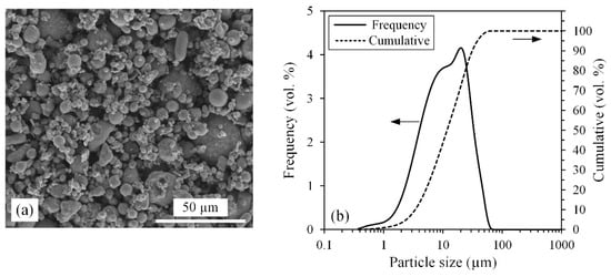
Figure 1.
(a) SEM observation and (b) particle size distribution of the 17-4 PH dry powder.
2.4.2. Feedstock Characterization
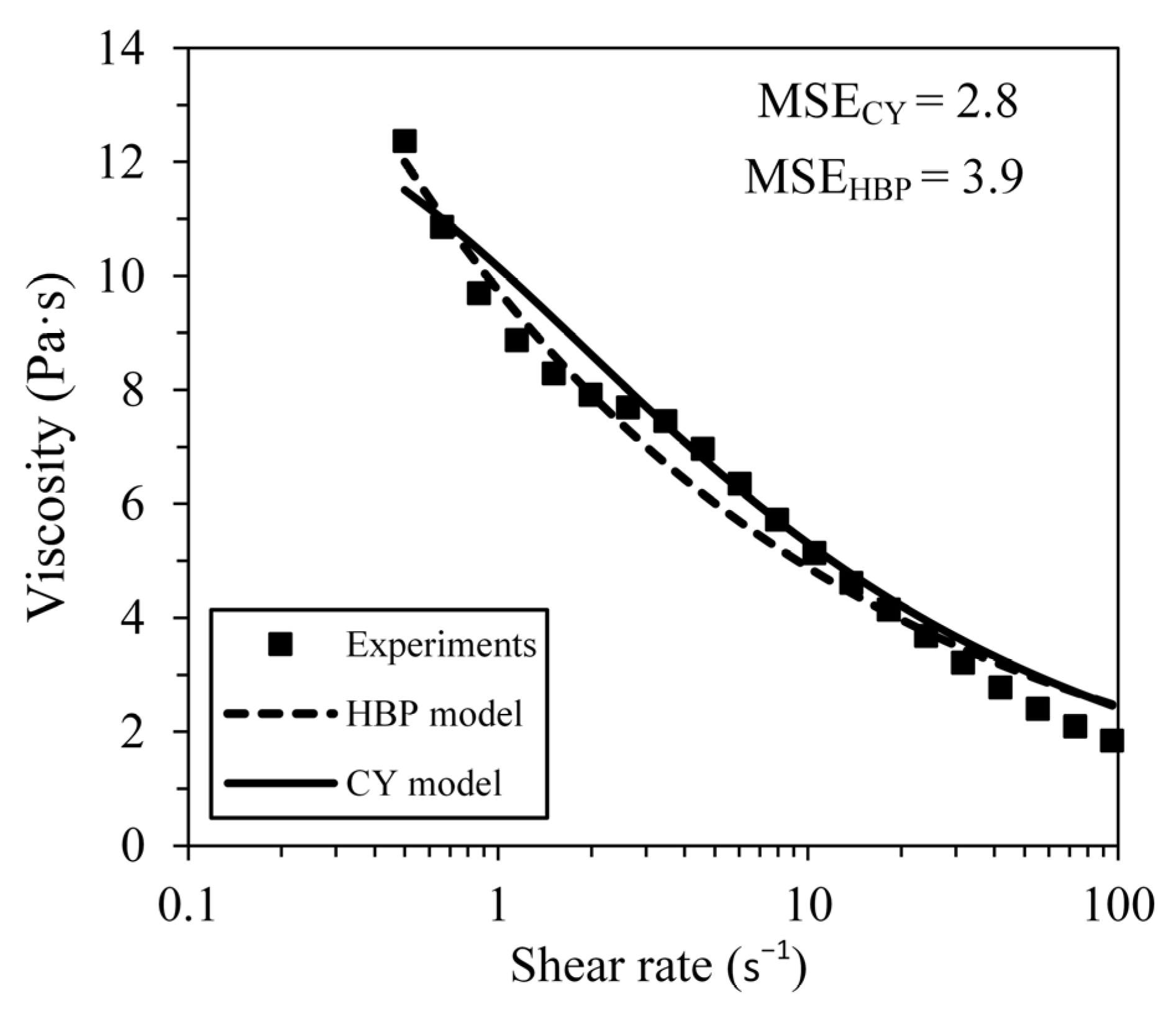
The viscosity profile was obtained at 90 °C using a MCR 302 rotational rheometer (Anton Paar, Graz, Austria) equipped with a CC-17 (cylinder and cup configuration) measuring tool and a C-PTD 200 temperature-controlled measuring system. The feedstock was preheated at 90 °C and then introduced in the rheometer cup before a shear deformation was applied at a rate ranging from 0.5 to 100 s−1. Experimental measurements were repeated three times to plot the average feedstock viscosity profile presented in Figure 2. The fitting parameters for the Herschel–Bulkley–Papanastasiou (HBP) and Carreau–Yasuda (CY) viscosity models reported in Table 1 were calculated by a fitting procedure using Minitab. These two rheological models, which are plotted in Figure 2, were then implemented into DualSPHysics using Equations (7) and (8).
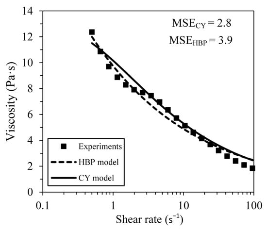
Figure 2.
Experimental viscosity data measured at 90 °C fitted by Herschel–Bulkley–Papanastasiou (HBP) and Carreau–Yasuda (CY) models along with mean square error (MSE) for shear deformation rate ranging from 1 to 20 s−1.

Table 1.
Fitting parameters used in the Carreau–Yasuda and Herschel–Bulkley–Papanastasiou viscosity models.
2.4.3. Mold Geometries and Real-Scale Injection Validation Setup
The numerical simulation results were validated by real-scale injections performed using the LPIM laboratory injection press illustrated in Figure 3a, and fully described in [52]. The feedstocks were heated up to 90 °C, and then injected into the mold cavities presented in Figure 3b,d to produce the rectangular and hourglass parts shown in Figure 3c,e. Following debinding and sintering treatment (not performed in the present study), these specimens can be machined to the proper dimension specified in ASTM E8 [53] and ASTM E466 [54] standards to obtain, respectively, the tensile and fatigue properties. During the calibration step of this work, the injections were performed into the rectangular shape at four different volumetric flow rates of 5.8, 7.8, 9.7, and 11.7 cm3/s. During the validation step, the injections were performed into the hourglass (convergent–divergent) shape using a constant volumetric flow rate of 7.8 cm3/s. The standard metallic mold upper plate was replaced by a transparent polycarbonate plate to visually record the filling process using a digital camera and recording was carried out with VirtualDub at 24 fps. The feedstock velocity was finally calculated from the captured videos using VLC. The experimental injection piston, cylinder, and rectangular mold cavity using were modeled by FreeCAD (Lesser General Public License) as a whole injection unit and imported into DualSPHysics.
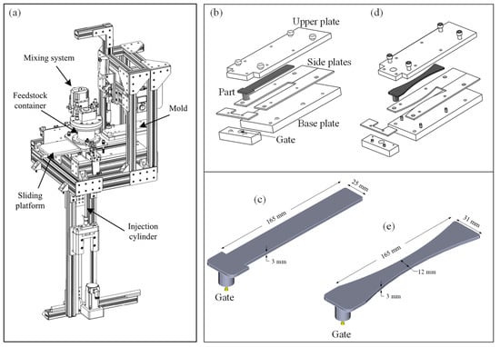
Figure 3.
(a) Laboratory injection press, (b,d) exploded view of the rectangular and hourglass mold cavities, and (c,e) overall dimensions of the injected parts (adapted from [55]).
3. Results and Discussion
3.1. Selection of the Viscosity Model
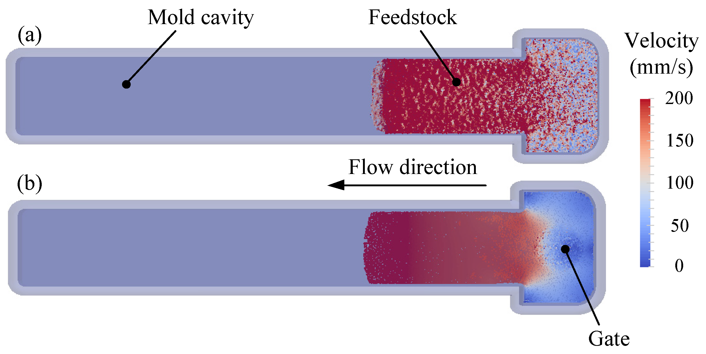
Figure 4 presents the numerical simulations for two short shots obtained using the same flow rates, but two different viscosity models. Note that these short shots represent the velocity field of the feedstock taken at 0.8 s, representing about 30% of the mold filling stage. As illustrated in Figure 3b,c, the feedstock enters by the gate through the larger section of the mold (i.e., normal to the top view reported in Figure 4) to finally fill the rectangular part using a volumetric flow rate of 7.8 cm3/s (i.e., from right to left on the top view reported in Figure 4). In Figure 4a, the velocity pattern obtained with the HBP model exhibits local and irregular rising and falling in the velocity of fluid particles. At a certain filling time (e.g., 0.8 s in this specific short shot), a constant feedstock velocity is expected through the rectangular part since the mold cavity cross-section remains constant. This non-uniform velocity color code thus represents an instability in the numerical solution. Such an instability may be attributed to the difficulties inherent in managing non-Newtonian flows in the SPH method. Indeed, the dependence of the viscosity on the shear deformation rate may well be problematic due to the fully explicit time integration nature of the SPH approach. For such a powder–binder feedstock, the shear thinning behavior may be responsible for a relatively large viscosity gradient for a small variation in the shear rate. Especially visible at low shear deformation rates, a fluid with a low flow behavior index n is expected to produce a significant increase in the feedstock viscosity for a small decrease in shear rate. According to Equation (7), the viscosity value tends to increase when the shear deformation rate decreases, thus constraining the time step length to ensure the stability of the solution. This problem becomes more severe in the simulation of fluids exhibiting lower values of n, due to the generation of strong viscous forces. In this respect, the HBP model appears to fail in providing stable results for feedstocks with n < 0.75. On the other hand, Figure 4b presents a numerical solution exhibiting a smooth and coherent transition of fluid particles in a mold without any sudden or punctual fluctuations in the velocity field of the feedstock. Based on Equation (8), the CY model produces lower viscosity variations when the shear deformation rate value decreases, and as a result, the length of the time step becomes less constrained than in the previous HBP model, and more stable results are seen. The CY viscosity model was thus selected to describe the complex shear thinning behavior of the feedstock. Therefore, instead of the HBP model already implemented in DualSPHysics, the CY viscosity model was implemented and used in this study as a viable option for representing the rheological behavior of the PIM feedstock in the SPH model. Finally, and as seen in Figure 2, the CY model produced a smaller mean squared error than the HBP model, especially at effective shear deformation rates ranging from 1 to 20 s−1.

Figure 4.
Top view of two simulated injections showing the velocity field of the feedstock using (a) the Herschel–Bulkley–Papanastasiou model, and (b) the Carreau–Yasuda model.
3.2. Selection of the Interparticle Distance
In the SPH method, the interparticle distance (IPD) is one of the most important parameters mapping the spatial distribution of particles. Much like the mesh size used in the finite element method, the IPD directly defines the number of particles in the problem, and drives the result accuracy and computational resources. Figure 5a presents the evolution of the simulated flow front length and computational time according to the IDP. As expected, an increase in IPD from 0.2 to 0.5 mm produces a proportional decrease in the computational time (of about five times). Also note that all increases in IDP above 0.4 mm significantly change the numerical response, with values of the flow front length increasing with an increase in IDP. As illustrated in the velocity field presented in Figure 5b, a too-high IDP value may also generate an unstable numerical solution combining local and irregular rising and falling in the fluid velocity, similar to the erratic pattern shown above in Figure 4a, when a non-suitable viscosity model is used. As explained by Lind et al. [56], an increase in IDP directly decreases the amount of interpolation points in the range of the kernel, causing a divergence in the numerical solution when the quantity of these interpolation points exceeds a certain threshold. As expected with such a convergence analysis, a decrease in the IDP changes the flow front length value up to the stabilization of these physical parameters. In the present work, all IDP ≤ 0.4 mm produces no significant impact on the simulated flow front length. In addition, refining the discretization of the domain also produces a direct impact on the accuracy of the SPH solution, with a smooth gradient seen in the feedstock velocity without any punctual or sudden change of this parameter over the injected part in Figure 5c. The results obtained in Figure 5b,c thus confirm that the resolution of the particle mapping drives both the accuracy and the stability of the numerical solution. Since an IDP of between 0.2–0.3 mm produces no significant gain in accuracy, but calls for a very high computational time, an IDP of 0.4 mm was selected for the rest of this study to guarantee accurate and stable simulation solutions, while requiring a decent computational time of about 40–50 h using the HPC described above.
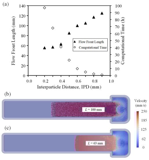
Figure 5.
(a) Evolution of the simulated flow front length and computational time according to the interparticle distance, and typical flow front lengths obtained for IPDs of (b) 0.6 mm and (c) 0.4 mm.
3.3. Selection of the Boundary Friction Factor
3.3.1. Friction Factor for a Low Injection Flow Rate
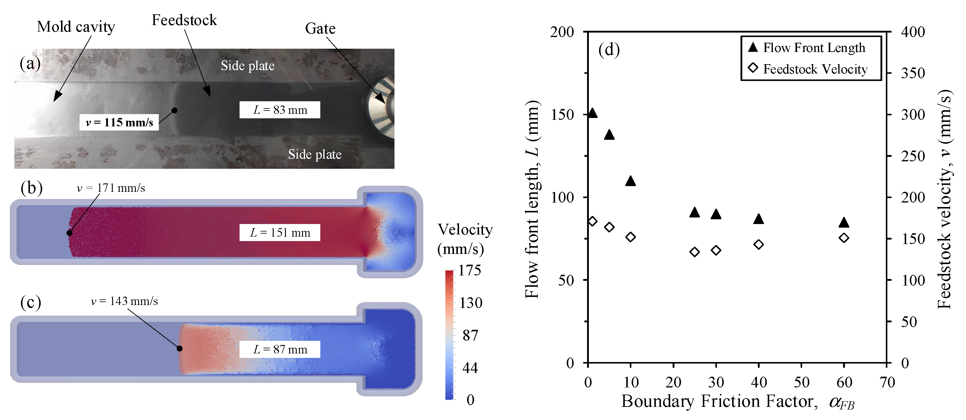
Figure 6 presents the experimental and simulation results obtained in the same rectangular cavity using a relatively low injection flow rate of 7.8 cm3/s. These tests were performed to calibrate the boundary friction factor () used in the modified conservation of momentum equation (Equation (6)) and to numerically capture the friction forces experienced by the feedstock during an injection. In other words, the factor was implemented in the code because, surprisingly, by default, DualSPHysics did not take into account the friction occurring between the feedstock and the mold cavity. To that end, two physical quantities, namely, the injected length (L) and feedstock velocity (v), were extracted from four experimental injections at an injection time of 1.6 s (Figure 6a) and compared to those obtained numerically with different values (Figure 6b–d). This factor has a non-zero and positive value (≥1) in order to artificially create friction at the interface between the feedstock and the mold surface. In other words, values of = 1 and > 1 represent frictionless and friction states, respectively. As illustrated in Figure 6b, no velocity reduction was observed near the mold–wall interface when the simulated feedstock encountered no friction at the walls ( = 1). Using this slip wall condition, the simulated injected length and the feedstock velocity were about 40 and 50% higher than those obtained experimentally. An increase in the boundary friction factor (e.g., = 25) clearly produces a reduction in particle velocity, with the thin blue band with a thickness varying from 0 to 1.4 mm being visible in Figure 6c. This zero-velocity condition at the wall confirms that the feedstock numerically encounters friction forces at the walls. In this case, the simulated injection length is approaching the experimental value, with a relative difference of about (87 mm − 83 mm)/83 mm = 5%. However, the use of a boundary friction factor does not appear to improve the velocity value, with a v = 143 mm/s, i.e., still 25% higher than that obtained experimentally. This latter conclusion is also visible in Figure 6d, where a threshold value of ≥ 25 stabilizes the injection length at a value close to the experimental one, but where the feedstock velocity predicted numerically remains too high at the flow front point. For this reason, the feedstock velocity was also analyzed at different points over the width and the thickness of the flow front.

Figure 6.
(a) Experimental and (b,c) simulated injected lengths (top views) obtained with boundary friction factors set at = 1 and 25, respectively, and (d) evolution of the flow length (L) and feedstock velocity (v) according to the factor (short shot obtained at t = 1.6 s using a volumetric flow rate of 7.8 cm3/s).
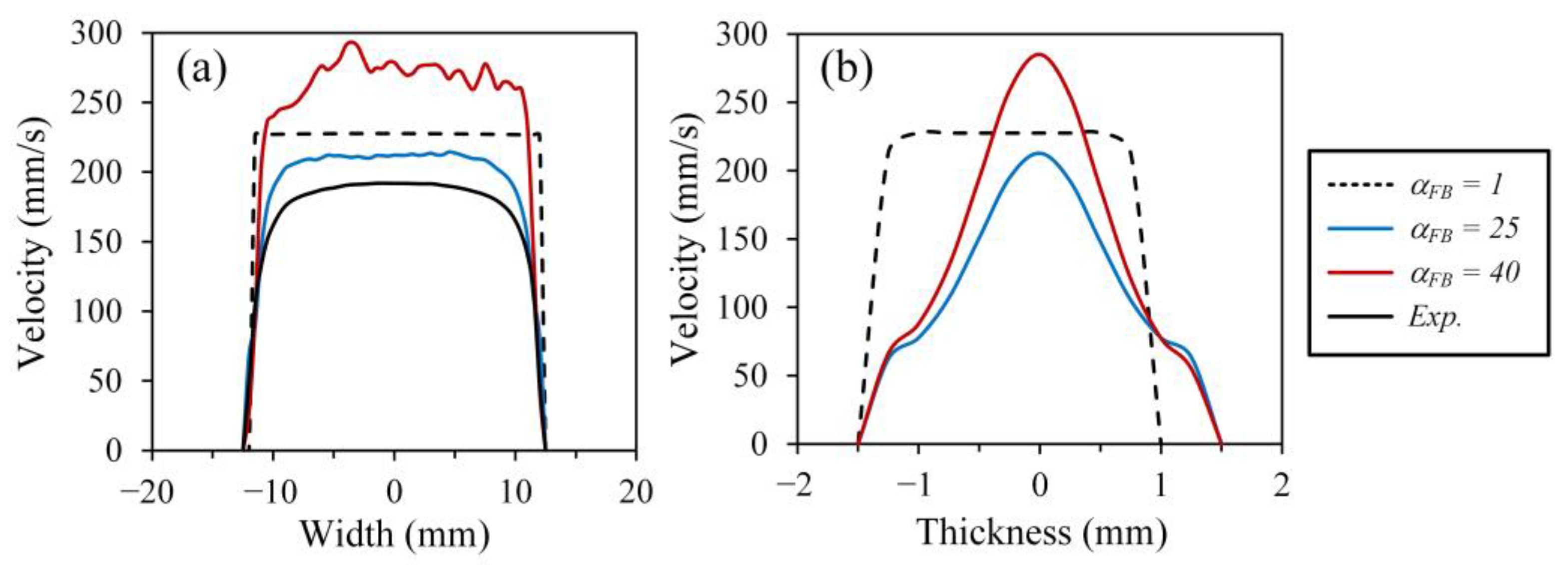
Figure 7a,b shows the flow velocity profiles along the width and thickness of the mold cross-section obtained at the flow front for different boundary friction factor values. As a reference, the width and thickness values refer to the 2D positions of the mold cross-section (illustrated in gray in Figure 7c) superimposed on a Cartesian plane (illustrated in black in Figure 7c), and extracted from the isometric view reported in Figure 7d. In Figure 7a,b, only the simulated velocity profiles obtained along the width at the surface of the mold were compared to the experimental result, because the values were simply impossible to experimentally measure along the thickness. In the no-friction condition ( = 1), the feedstock reaches a maximum flow front velocity throughout the mold. In addition, the velocity profile across the width (Figure 7a) is abnormally flat, meaning that fluid particles close to the mold wall exhibit the same velocities as the fluid particles far from the wall. Also at the feedstock–wall interface, the absence of any reduction in fluid velocity confirms a free-slip condition. The velocity profile also exhibits a pronounced filling imbalance over the thickness, leading to an incomplete mold filling, where the feedstock, simulated using this condition, never touches the upper surface of the mold (Figure 7b). In other words, feedstock is not able to vertically fill the whole mold thickness due to this high velocity. Combined with the excessive injection length seen above in Figure 6b, this incomplete mold filling is similar to the jetting phenomenon observed in PIM when the injection flow rate is too high.
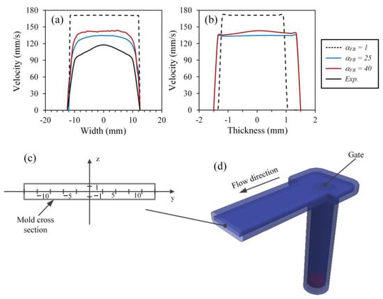
Figure 7.
Velocity profiles obtained using different boundary friction factors along (a) the width of the mold and (b) the thickness of the mold, and (c) cross-section of the mold superimposed on a Cartesian plane extracted from (d) the isometric view (short shot obtained at t = 1.6 s using a volumetric flow rate of 7.8 cm3/s).
If the boundary friction factor is increased to = 25, the evolution of the velocity along the width shows an expected profile exhibiting a maximum velocity in mid-width flow that gradually decreases near the mold wall, as illustrated in Figure 7a. Confirming the results obtained above, the maximum value, but also the velocity profile simulated using this boundary friction factor, are close to those obtained experimentally. In addition, the mold filling over the thickness is balanced where the feedstock now touches the base plate as well as the upper plate of the mold walls (Figure 7b). Further increases in the boundary friction factor, e.g., up to = 40, lead to a greater difference with the experimental results and to a loss in stability of the numerical solution, with abnormal noises seen in the velocity profile (Figure 7a). As expected, the whole profile along the thickness shows a higher velocity in the center of the mold thickness (confirming the effect of friction on velocity), and the maximum simulated velocity at = 40 is slightly higher than that obtained at = 25. To achieve reasonable results for both the velocity profile and the flow length, it seems that the appropriate value of the boundary friction factor should be = 25. This value will be used in DualSPHysics for the rest of this work.
3.3.2. Validation of the Friction Factor for a High Injection Flow Rate
A similar analysis was repeated using a higher injection flow rate of 19.5 cm3/s (i.e., 2.5 times higher than the previous section) in order to confirm whether the optimal boundary friction factor = 25 can be used for any flow rate range. Figure 8a–c show the experimental and simulated flow front length (L) obtained for different boundary friction factors in the same rectangular mold cavity, but in this case, 0.8 s after the injection process was started. These results show that the boundary friction factor has developed similar trends even at higher injection flow rates and confirms the effectiveness of the boundary friction factor when it comes to creating a friction state at the wall. The overall differences between the injected lengths and feedstock velocity predicted numerically remain low when a boundary friction factor of about = 25 is used. The viscous forces between the fluid particles are governed by the viscosity of the fluid and the friction state at the mold surface. Since the feedstock viscosity at high and low injection rates is expected to be different, the influence of the boundary friction factor on the flow front length and feedstock velocity at high and low injection rates is also expected to be different. However, and as seen in Figure 8d, the optimal set at 25 produces a plateau-like trend for the flow front length varying from 122–133 mm and the feedstock velocity varying from 212–227 mm/s, meaning that this optimal boundary friction factor can be used over the whole injection flow rate range.
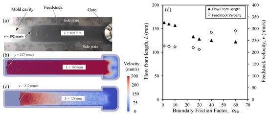
Figure 8.
(a) Experimental and (b,c) simulated injected lengths (top views) obtained with boundary friction factors set at = 1 and 25, respectively, and (d) evolution of the flow length (L) and feedstock velocity (v) according to the factor (short shot obtained at t = 0.8 s using a volumetric flow rate of 19.5 cm3/s).
Using a high flow rate of 19.5 cm3/s, Figure 9 presents the velocity profiles obtained at 0.8 s along the width and thickness of the mold cross-section, calculated at the flow front for different boundary friction factor values. Note that the same Cartesian coordinate system presented in Figure 7c was used to build Figure 9. When = 1, the same free-slip condition trend was seen where the velocity near the mold walls is similar to that observed along the thickness (Figure 9a). In this SPH particle formulation, this boundary friction factor implies that the friction between the fluid particles and wall particles is similar to that between the fluid particles far from the mold surface, even though the wall particles are stationary. In addition, the similar filling imbalance as that observed at low flow rates was seen over the thickness direction (Figure 9b). In addition to the fluid particle deceleration observed near the walls along the thickness, this unbalanced filling was completely prevented when any boundary friction factor was used (e.g., = 25 or 40). Setting = 25, a decrease in the velocity of fluid particles close to the wall can be observed along the width. In addition, a decrease in the maximum velocity towards the values obtained experimentally was visible. However, the velocity profile obtained along the width exhibits an unexpected noise similar to that obtained previously (with low flow rates and higher boundary friction factor reported in Figure 7). A further increase in the boundary friction factor generated significant oscillations in the transverse velocity profile, which is an indication of stability deterioration. Although = 25 produced relevant injection results even at high flow rates, this suggests that the boundary friction factor may need to be slightly adjusted according to the flow rate. The latter value may subsequently need to be implemented as a matrix or a material law in DualSPHysics, i.e., similarly to the rheological properties.
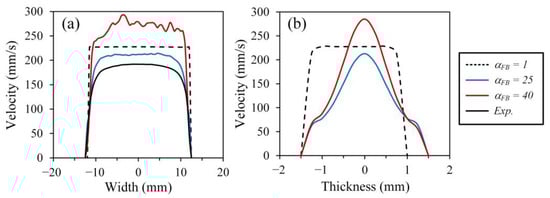
Figure 9.
Velocity profiles obtained using different boundary friction factors along (a) the width of the mold, and (b) the thickness of the mold (short shot obtained at t = 0.8 s using a volumetric flow rate of 19.5 cm3/s).
3.4. Validation of the SPH Model to Simulate PIM Injections
The capacity of the modified SPH model developed in this work to simulate the PIM injection process was validated using experimental measurements. To that end, the optimal boundary friction factor defined above was set at = 25 and new simulations were performed in the more complex mold cavity exhibiting the hourglass shape presented in Figure 3d,e. Using a constant volumetric flow rate of 7.8 cm3/s, the convergent and divergent channel presented in Figure 10a,b was used to capture the injection length (L) and flow front velocity (v) at t = 1.6 s. On the one hand, the simulated flow front length obtained with this acceleration-deceleration pattern intrinsically linked with this hourglass mold (Figure 10b) agreed well with the experimental results (Figure 10a), with a relative difference of about 12%. However, this relatively low difference in the two injected lengths (noted ∆L in Figure 10a,b) produces different widths for the velocity profiles presented in Figure 10d. On the other hand, the velocity field presented in Figure 10b confirms that the feedstock encounters friction forces near the walls, where a thin blue band is still visible in this mold. A zoom-in of this specific zone presented in Figure 10c confirms that this frictional effect occurred without any signs of numerical instability. In this respect, the flow front velocity obtained numerically was also close to the experimental value, with a relative difference lower than 15%.
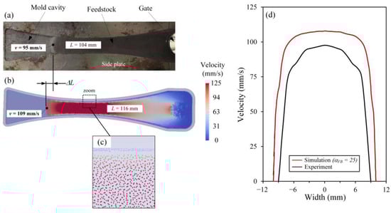
Figure 10.
(a,b) Experimental and simulated injected lengths (top views), (c) zoom-in of the fluid particles close to the wall of the mold, and (d) experimental and simulated velocity profiles along the width ( = 25; short shot obtained at t = 1.6 s using a volumetric flow rate of 7.8 cm3/s).
Interestingly, the velocity profiles presented in Figure 10d are slightly different. This difference between the experimental and simulation results could be explained by the heat transfer phenomenon, which is not taken into account in the SPH model (which could also explain the difference seen above for the rectangular mold), but also by the variation of the boundary friction factor in more complex molds. Indeed, the acceleration–deceleration flow pattern experienced by the feedstock could generate changes in the friction state at the wall that are a function of viscous forces between particles. In fact, in the original SPH code, the friction force created between the wall and the fluid is of the same type and magnitude as that between the fluid particles, meaning that the friction at the interface wall/feedstock is probably not generated uniformly in the different areas of such more complex molds (i.e., dependent of the feedstock velocity, and thus producing a different shear rate leading to different feedstock viscosity). With a constant boundary friction factor applied, the friction forces at this boundary should therefore differ slightly from the real friction state experienced by the feedstock experimentally. In other words, if larger viscous forces are developed between the fluid particles, frictional forces, and, thus, the artificial boundary friction factor, should be increased, and vice versa. In addition to the aforementioned hypotheses, there are several other factors that may influence the accuracy of the SPH results. These factors are directly linked to the main challenges of the SPH method, namely: (i) convergence, consistency, and stability, (ii) boundary conditions, (iii) adaptivity, and (iv) coupling to other models. That might include the rheological model, IPD, kernel function, time integration scheme, etc.
During a PIM injection stage, the feedstock is surrounded by mold walls imposing specific conditions to the flow. In DualSPHysics, the original code contains the dynamic boundary condition (DBC) method for managing solid boundaries, and, ultimately, the interaction of the fluid with the walls within the numerical domain. In this method, the boundaries are defined by a set of SPH particles considered distinct from the fluid particles for which no displacement may occur even if they are subjected to external forces. The results obtained in this work revealed that the DBC method alone (i.e., = 1.) was not able to capture the no-slip boundary occurring at the mold surfaces, leading to a feedstock velocity that was significantly higher than that expected near to and far from the mold walls. In this respect, the modified conservation of momentum proposed in Equation (6) produces a sort of artificial friction near the mold walls, significantly improving the accuracy of the feedstock velocity and injection length obtained numerically. The optimal frictional effect, as well as the stability of the numerical solution, were obtained for = 25 regardless of the flow rate to decrease the numerical error by two to three times.
4. Conclusions
In this study, the ability of a meshless numerical method based on smoothed particle hydrodynamics (SPH) was demonstrated for simulating the injection phase in powder injection molding. Flow patterns and velocity fields were simulated on the DualSPHysics platform using a modified conservation of momentum equation involving a new boundary friction factor (). Since the original SPH code fails to impose a no-slip boundary condition at the mold interface, a value set at = 25 produced both an optimal frictional effect and stability of the numerical solution, thus preventing unrealistic imbalance filling, inconsistent injected lengths, and excessive velocities, as compared to the experimental results. Near the mold surface, this conditional modification of the viscous term in the momentum equation also positively modified the velocity profile of the feedstock along the width and thickness of the mold. The rheological model implemented by default in the native code was also modified to better describe the non-Newtonian behavior of the powder–binder mixture used in this study. By combining the optimal boundary friction factor and rheological model, this work confirmed that the SPH approach can be successfully used to numerically predict the injection stage of the powder injection molding process. The flow front length and feedstock velocity obtained in a complex cavity (hourglass shape) were satisfactorily predicted with relative differences of 12 and 15%, respectively.
Author Contributions
Conceptualization, V.D. and S.M.; methodology, V.D. and L.D.; software, S.M.; validation, S.M. and V.D; formal analysis, V.D. and L.D.; investigation, S.M.; resources, S.M.; data curation, S.M.; writing—original draft preparation, S.M.; writing—review and editing, V.D.; visualization, S.M.; supervision, V.D. and L.D.; project administration, V.D.; funding acquisition, V.D. All authors have read and agreed to the published version of the manuscript.
Funding
This research was carried out with the financial support of the Natural Science and Engineering Research Council (NSERC, RGPIN-2018-04407).
Data Availability Statement
The data presented in this study are available on request from the corresponding author.
Conflicts of Interest
The authors declare no conflict of interest.
References
- Heaney, D.F. Handbook of Metal Injection Molding; Woodhead Publishing: Sawston, UK, 2012; ISBN 9780857096234. [Google Scholar]
- González-gutiérrez, J.; Beulke Stringari, G.; Emri, I.; Stringari, G.B.; Emri, I. Powder Injection Molding of Metal and Ceramic Parts; IntechOpen: London, UK, 2012; ISBN 978-953-51-0297-7. [Google Scholar]
- Yarlagadda, P.K.D.V. Development of an Integrated Neural Network System for Prediction of Process Parameters in Metal Injection Moulding. J. Mater. Process. Technol. 2002, 130–131, 315–320. [Google Scholar] [CrossRef]
- Bilovol, V.V.; Kowalski, L.; Duszczyk, J.; Katgerman, L.; Bilovol, V.V.; Kowalski, L.; Duszczyk, J.; Katgerman, L. Comparison of Numerical Codes for Simulation of Powder Injection Moulding. Powder Metall. 2003, 46, 55–60. [Google Scholar] [CrossRef]
- Zheng, Z.S.; Qu, X.H. Numerical Simulation of Powder Injection Moulding Filling Process for Intricate Parts Numerical Simulation of Powder Injection Moulding Filling Process for Intricate Parts. Powder Metall. 2006, 49, 167–172. [Google Scholar] [CrossRef]
- Aggarwal, G.; Park, S.J.; Smid, I. Development of Niobium Powder Injection Molding: Part I. Feedstock and Injection Molding. Int. J. Refract. Met. Hard Mater. 2006, 24, 253–262. [Google Scholar] [CrossRef]
- Ahn, S.; Chung, S.T.; Atre, S.V.; Park, S.J.; German, R.M.; Chung, S.T.; Atre, S.V.; Park, S.J.; Integrated, R.M.G.; Ahn, S.; et al. Integrated Filling, Packing and Cooling CAE Analysis of Powder Injection Moulding Parts Integrated Filling, Packing and Cooling CAE Analysis of Powder Injection Moulding Parts. Powder Metall. 2008, 51, 318–326. [Google Scholar] [CrossRef]
- Urval, R.; Lee, S.; Atre, S.V.; Park, S.; German, R.M.; Lee, S.; Atre, S.V.; Park, S.; Optimisation, R.M.G.; Urval, R.; et al. Optimisation of Process Conditions in Powder Injection Moulding of Microsystem Components Using a Robust Design Method: Part I. Primary Design Parameters. Powder Metall. 2008, 51, 133–142. [Google Scholar] [CrossRef]
- Ahn, S.; Park, S.J.; Lee, S.; Atre, S.V.; German, R.M. Effect of Powders and Binders on Material Properties and Molding Parameters in Iron and Stainless Steel Powder Injection Molding Process. Powder Technol. 2009, 193, 162–169. [Google Scholar] [CrossRef]
- Kate, K.H.; Enneti, R.K.; Onbattuvelli, V.P.; Atre, S.V. Feedstock Properties and Injection Molding Simulations of Bimodal Mixtures of Nanoscale and Microscale Aluminum Nitride. Ceram. Int. 2013, 39, 6887–6897. [Google Scholar] [CrossRef]
- Lenz, J.; Enneti, R.K.; Park, S.J.; Atre, S.V. Powder Injection Molding Process Design for UAV Engine Components Using Nanoscale Silicon Nitride Powders. Ceram. Int. 2014, 40, 893–900. [Google Scholar] [CrossRef]
- Kim, J.; Ahn, S.; Atre, S.V.; Park, S.J.; Kang, T.G.; German, R.M. Imbalance Filling Ofmulti-Cavity Tooling during Powder Injection Molding. Powder Technol. 2014, 257, 124–131. [Google Scholar] [CrossRef]
- Sardarian, M.; Mirzaee, O.; Habibolahzadeh, A. Numerical Simulation and Experimental Investigation on Jetting Phenomenon in Low Pressure Injection Molding (LPIM) of Alumina. J. Mater. Process. Tech. 2017, 243, 374–380. [Google Scholar] [CrossRef]
- Sardarian, M.; Mirzaee, O.; Habibolahzadeh, A. Influence of Injection Temperature and Pressure on the Properties of Alumina Parts Fabricated by Low Pressure Injection Molding (LPIM). Ceram. Int. 2017, 43, 4785–4793. [Google Scholar] [CrossRef]
- Sardarian, M.; Mirzaee, O.; Habibolahzadeh, A. Mold Filling Simulation of Low Pressure Injection Molding (LPIM) of Alumina: Effect of Temperature and Pressure. Ceram. Int. 2017, 43, 28–34. [Google Scholar] [CrossRef]
- Azzouni, M.; Demers, V.; Dufresne, L. Mold Filling Simulation and Experimental Investigation of Metallic Feedstock Used in Low-Pressure Powder Injection Molding. Int. J. Mater. Form. 2021, 14, 961–972. [Google Scholar] [CrossRef]
- Ye, T.; Pan, D.; Huang, C.; Liu, M. Smoothed Particle Hydrodynamics (SPH) for Complex Fluid Flows: Recent Developments in Methodology and Applications. Phys. Fluids 2019, 31, 011301. [Google Scholar] [CrossRef]
- Liu, M.B.; Liu, G. Smoothed Particle Hydrodynamics (SPH): An Overview and Recent Developments. Arch. Comput. Methods Eng. 2010, 17, 25–76. [Google Scholar] [CrossRef]
- Hosain, M.L.; Fdhila, R.B. Literature Review of Accelerated CFD Simulation Methods towards Online Application. Energy Procedia 2015, 75, 3307–3314. [Google Scholar] [CrossRef]
- Xu, X.; Ouyang, J.; Yang, B.; Liu, Z. SPH Simulations of Three-Dimensional Non-Newtonian Free Surface Flows. Comput. Methods Appl. Mech. Eng. 2013, 256, 101–116. [Google Scholar] [CrossRef]
- Shadloo, M.S.; Oger, G.; Le Touzé, D. Smoothed Particle Hydrodynamics Method for Fluid Flows, towards Industrial Applications: Motivations, Current State, And Challenges. Comput. Fluids 2016, 136, 11–34. [Google Scholar] [CrossRef]
- Monaghan, J.J. Smoothed Particle Hydrodynamics and Its Diverse Applications. Annu. Rev. Fluid Mech. 2012, 44, 323–346. [Google Scholar] [CrossRef]
- Cleary, P.; Prakash, M.; Ha, J.; Sinnott, M.; Nguyen, T.; Grandfield, J.; Hydrodynamics, S.; Cleary, P.; Prakash, M.; Ha, J.; et al. Modeling of Cast Systems Using Smoothed-Particle Hydrodynamics. JOM 2004, 56, 67–70. [Google Scholar] [CrossRef]
- Hu, M.Y.; Cai, J.J.; Li, N.; Yu, H.L.; Zhang, Y.; Sun, B.; Sun, W.L. Flow Modeling in High-Pressure Die-Casting Processes Using SPH Model. Int. J. Met. 2018, 12, 97–105. [Google Scholar] [CrossRef]
- Cleary, P.W.; Ha, J.; Prakash, M.; Nguyen, T. 3D SPH Flow Predictions and Validation for High Pressure Die Casting of Automotive Components. Appl. Math. Model. 2006, 30, 1406–1427. [Google Scholar] [CrossRef]
- Cleary, P.W. Extension of SPH to Predict Feeding, Freezing and Defect Creation in Low Pressure Die Casting. Appl. Math. Model. 2010, 34, 3189–3201. [Google Scholar] [CrossRef]
- Cleary, P.; Ha, J.; Alguine, V.; Nguyen, T. Flow Modelling in Casting Processes. Appl. Math. Model. 2002, 26, 171–190. [Google Scholar] [CrossRef]
- Ellingsen, K.; Coudert, T.; M’Hamdi, M. SPH Based Modelling of Oxide and Oxide Film Formation in Gravity Die Castings. IOP Conf. Ser. Mater. Sci. Eng. 2015, 84, 012064. [Google Scholar] [CrossRef]
- Cleary, P.W.; Prakash, M.; Ha, J. Novel Applications of Smoothed Particle Hydrodynamics (SPH) in Metal Forming. J. Mater. Process. Technol. 2006, 177, 41–48. [Google Scholar] [CrossRef]
- Afrasiabi, M.; Luthi, C.; Bambach, M.; Wegener, K. Smoothed Particle Hydrodynamics Modeling of the Multi-layer Laser Powder Bed Fusion Process. Procedia CIRP 2022, 107, 276–282. [Google Scholar] [CrossRef]
- Dao, M.H.; Lou, J. Simulations of Laser Assisted Additive Manufacturing by Smoothed Particle Hydrodynamics. Comput. Methods Appl. Mech. Eng. 2021, 373, 113491. [Google Scholar] [CrossRef]
- Long, T.; Huang, H. An improved high order smoothed particle hydrodynamics method for numerical simulations of selective laser melting process. Eng. Anal. Bound. Elem. 2023, 147, 320–335. [Google Scholar] [CrossRef]
- Ichimiya, M.; Yamagata, N. High Viscous Flow Analysis in the 3D Printer by SPH. Mech. Mach. Sci. 2020, 75, 309–317. [Google Scholar] [CrossRef]
- Zhang, Z.; Shu, C.; Khalid, M.S.U.; Liu, Y.; Yuan, Z.; Jiang, Q.; Liu, W. SPH modeling and investigation of cold spray additive manufacturing with multi-layer multi-track powders. J. Manuf. Process. 2022, 84, 565–586. [Google Scholar] [CrossRef]
- Kiselev, S.P.; Kiselev, V.P.; Vorozhtsov, E.V. Smoothed Particle Hydrodynamics Method Used for Numerical Simulation of Impact Between an Aluminum Particle and a Titanium Target. J. Appl. Mech. Tech. Phys. 2022, 63, 1035–1049. [Google Scholar] [CrossRef]
- Lee, J.; Subedi, K.K.; Huang, G.W.; Lee, J.; Kong, S.-C. Numerical Investigation of YSZ Droplet Impact on a Heated Wall for Thermal Spray Application. J. Therm. Spray Technol. 2022, 31, 2039–2049. [Google Scholar] [CrossRef]
- Chaussonnet, G.; Dauch, T.; Keller, M.; Okraschevski, M.; Ates, C.; Schwitzke, C.; Koch, R.; Bauer, H.J. Progress in the Smoothed Particle Hydrodynamics Method to Simulate and Post-process Numerical Simulations of Annular Airblast Atomizers. Flow Turbul. Combust. 2020, 105, 1119–1147. [Google Scholar] [CrossRef]
- Guo, X.-G.; Li, M.; Dong, Z.-G.; Zhai, R.-F.; Jin, Z.-J.; Kang, R.-K. Smooth particle hydrodynamics modeling of cutting force in milling process of TC4. Adv. Manuf. 2019, 7, 364–373. [Google Scholar] [CrossRef]
- Falcone, M.; Buss, L.; Fritsching, U. Model assessment of an open-source smoothed particle hydrodynamics (SPH) simulation of a vibration-assisted drilling process. Fluids 2022, 7, 189. [Google Scholar] [CrossRef]
- Fan, X.-J.; Tanner, R.I.; Zheng, R. Smoothed Particle Hydrodynamics Simulation of Non-Newtonian Moulding Flow. J. Nonnewton. Fluid Mech. 2010, 165, 219–226. [Google Scholar] [CrossRef]
- Xu, X.; Yu, P. Modeling and Simulation of Injection Molding Process of Polymer Melt by a Robust SPH Method. Appl. Math. Model. 2017, 48, 384–409. [Google Scholar] [CrossRef]
- Xu, X.; Yu, P. Extension of SPH to Simulate Non-Isothermal Free Surface Flows during the Injection Molding Process. Appl. Math. Model. 2019, 73, 715–731. [Google Scholar] [CrossRef]
- He, L.; Lu, G.; Chen, D.; Li, W.; Chen, L.; Yuan, J.; Lu, C. Smoothed Particle Hydrodynamics Simulation for Injection Molding Flow of Short Fiber-Reinforced Polymer Composites. J. Compos. Mater. 2018, 52, 1531–1539. [Google Scholar] [CrossRef]
- Greiner, A.; Kauzlari, D.; Korvink, J.G.; Heldele, R.; Schulz, M.; Piotter, V.; Hanemann, T.; Weber, O.; Haußelt, J. Simulation of Micro Powder Injection Moulding: Powder Segregation and Yield Stress Effects during Form Filling. J. Eur. Ceram. Soc. 2011, 31, 2525–2534. [Google Scholar] [CrossRef]
- Lind, S.J.; Rogers, B.D.; Stansby, P.K. Review of Smoothed Particle Hydrodynamics: Towards Converged Lagrangian Flow Modelling. Proc. R. Soc. A Math. Phys. Eng. Sci. 2020, 476, 20190801. [Google Scholar] [CrossRef]
- Kauzlarić, D.; Pastewka, L.; Bretthauer, C.; Greiner, A.; Jan, G.K. SPH Simulation of the Embossing and Injection Moulding of Micro-Parts: Softening and Aggregation Aspects. In Proceedings of the 3rd International Conference on Multi-Material Micro Manufacture, 4M 2007; Whittles: Dunbeath, UK, 2007; pp. 23–29. [Google Scholar]
- Fourtakas, G.; Rogers, B.D. Modelling Multi-Phase Liquid-Sediment Scour and Resuspension Induced by Rapid Flows Using Smoothed Particle Hydrodynamics (SPH) Accelerated with a Graphics Processing Unit (GPU). Adv. Water Resour. 2016, 92, 186–199. [Google Scholar] [CrossRef]
- Mokos, A.D. Multi-Phase Modelling of Violent Hydrodynamics Using Smoothed Particle Hydrodynamics (SPH) on Graphics Processing Units (GPUs). Ph.D. Thesis, University of Manchester, Manchester, UK, 2014. [Google Scholar]
- Kauzlarić, D.; Pastewka, L.; Meyer, H.; Heldele, R.; Schulz, M.; Weber, O.; Piotter, V.; Hausselt, J.; Greiner, A.; Korvink, J.G.; et al. Smoothed Particle Hydrodynamics Simulation of Shear-Induced Powder Migration in Injection Moulding. Philos. Trans. R. Soc. A Math. Phys. Eng. Sci. 2011, 369, 2320–2328. [Google Scholar] [CrossRef] [PubMed]
- Demers, V.; Fareh, F.; Turenne, S.; Demarquette, N.R.; Scalzo, O. Experimental study on moldability and segregation of Inconel 718 feedstocks used in low-pressure powder injection molding. Adv. Powder Technol. 2018, 29, 180–190. [Google Scholar] [CrossRef]
- Poh, L.; Della, C.; Ying, S.; Goh, C.; Li, Y. Powder distribution on powder injection moulding of ceramic green compacts using thermogravimetric analysis and differential scanning calorimetry. Powder Technol. 2018, 328, 256–263. [Google Scholar] [CrossRef]
- Lamarre, S.G.; Demers, V.; Chatelain, J.F. Low-Pressure Powder Injection Molding Using an Innovative Injection Press Concept. Int. J. Adv. Manuf. Technol. 2017, 91, 2595–2605. [Google Scholar] [CrossRef]
- ASTM-E8/E8M; Standard Test Methods for Tension Testing of Metallic Materials. ASTM International: West Conshohocken, PA, USA, 2022. [CrossRef]
- ASTM-E466; Standard Practice for Conducting Force Controlled Constant Amplitude Axial Fatigue Tests of Metallic Materials. ASTM International: West Conshohocken, PA, USA, 2021. [CrossRef]
- Arès, F. Influence des Paramètres D’injection sur la Pression dans un Moule et sur la Qualité des Pieces à Vert 662 en LPIM. Master’s Thesis, École de Technologie Supérieure, Montreal, QC, Canada, 27 October 2022. [Google Scholar]
- Lind, S.J.; Stansby, P.K.; Rogers, B.D.; Lloyd, P.M. Numerical Predictions of Water-Air Wave Slam Using Incompressible-Compressible Smoothed Particle Hydrodynamics. Appl. Ocean Res. 2015, 49, 57–71. [Google Scholar] [CrossRef]


Disclaimer/Publisher’s Note: The statements, opinions and data contained in all publications are solely those of the individual author(s) and contributor(s) and not of MDPI and/or the editor(s). MDPI and/or the editor(s) disclaim responsibility for any injury to people or property resulting from any ideas, methods, instructions or products referred to in the content. |
© 2023 by the authors. Licensee MDPI, Basel, Switzerland. This article is an open access article distributed under the terms and conditions of the Creative Commons Attribution (CC BY) license (https://creativecommons.org/licenses/by/4.0/).