
Deep Learning-Based Ultrasonic Testing to Evaluate the Porosity of Additively Manufactured Parts with Rough Surfaces


Abstract
1. Introduction
2. Experiments
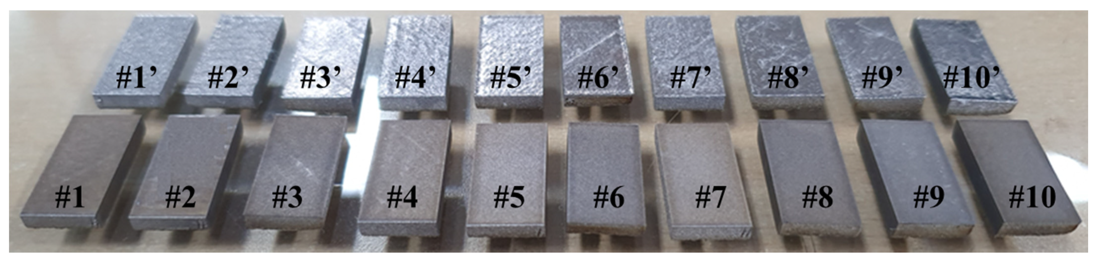
2.1. Fabrication of Porosity-Induced Specimens with Different Levels of Surface Roughness
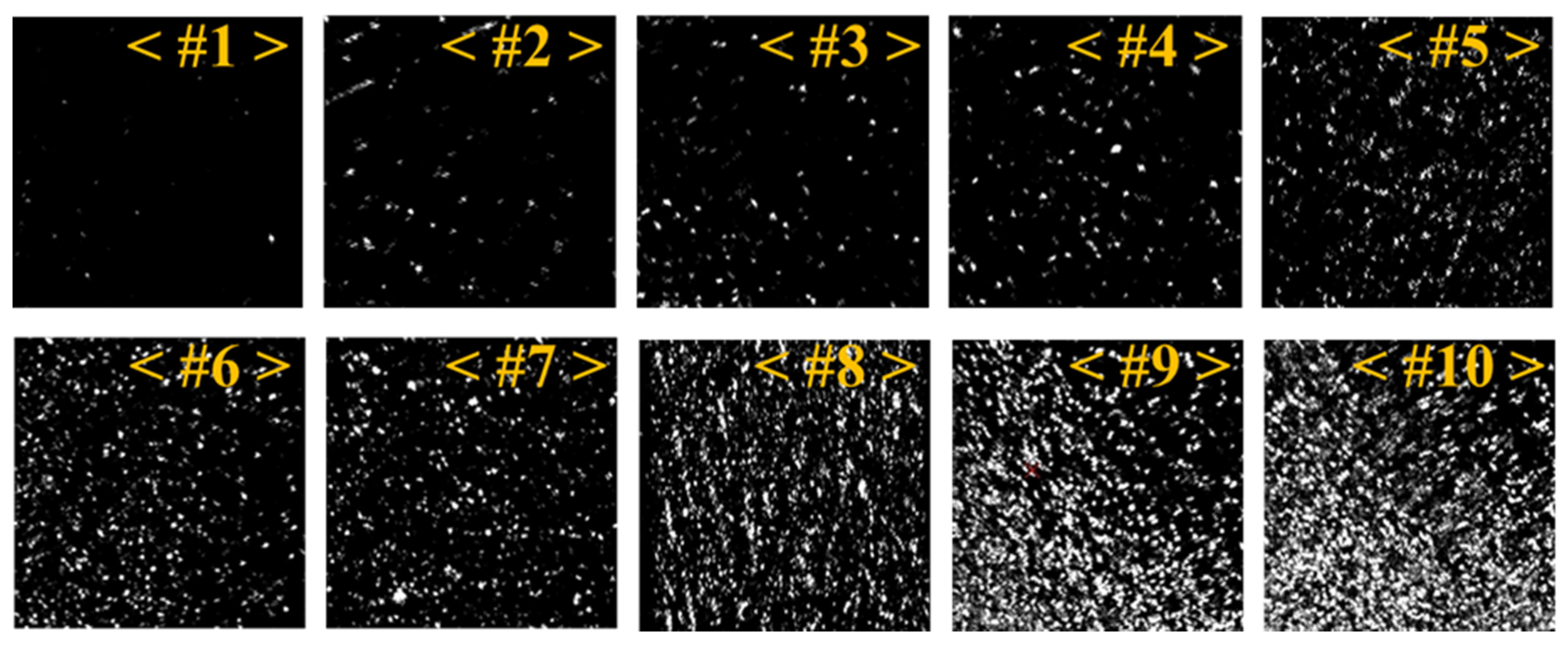
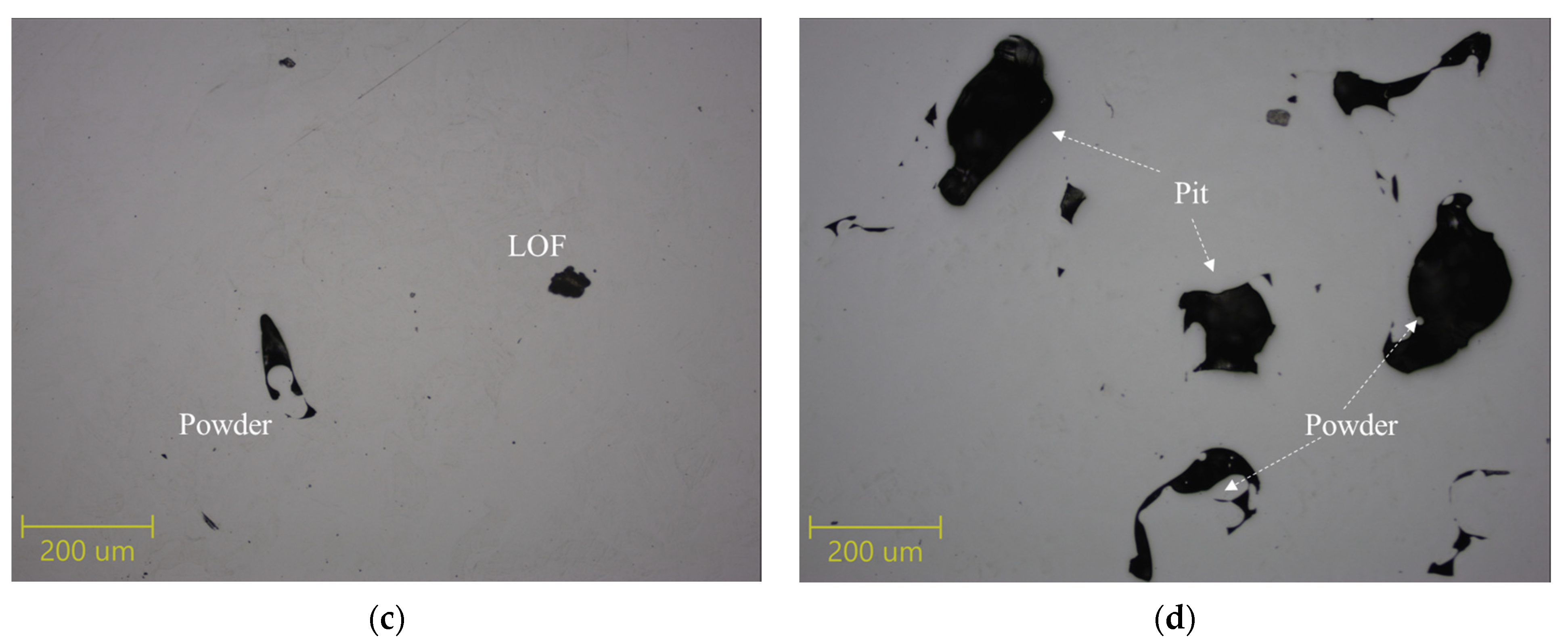
2.2. Porosity Examination
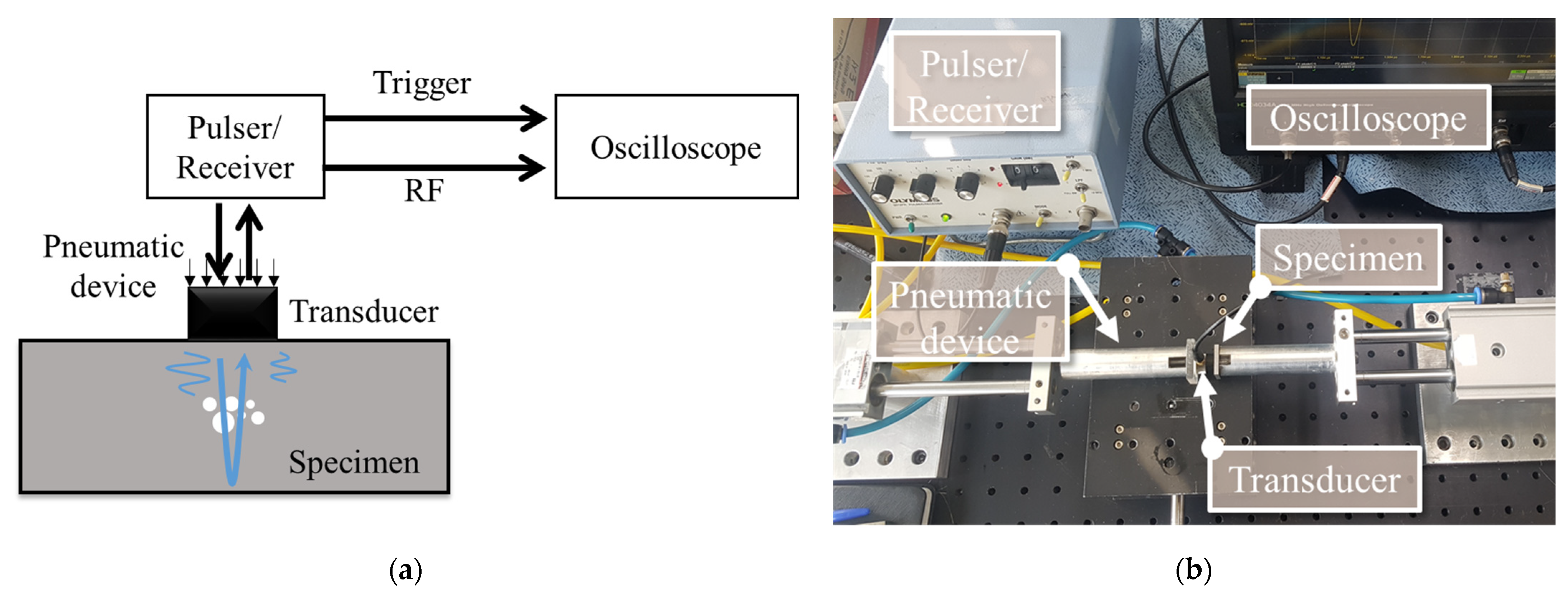
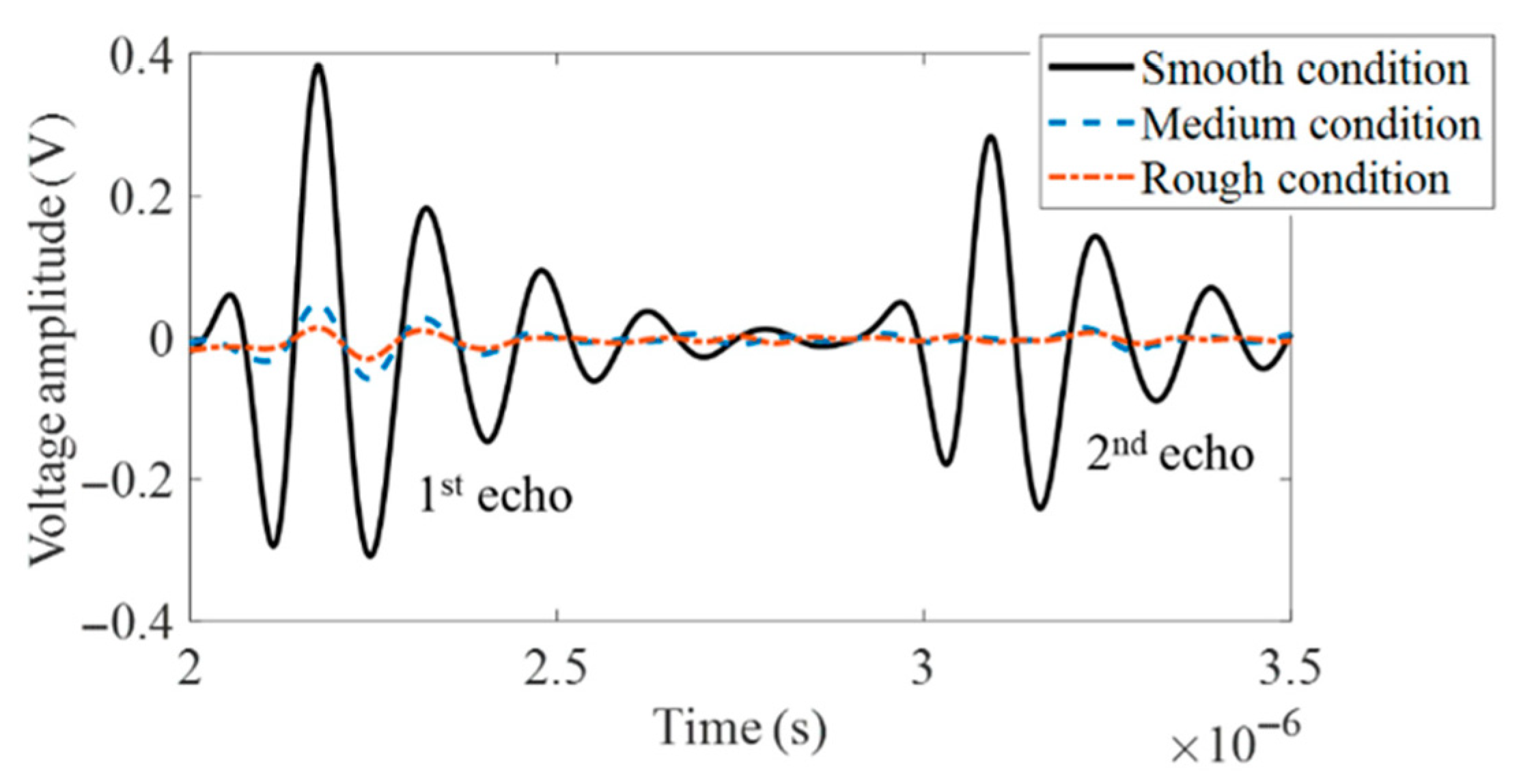
2.3. Ultrasonic Measurements
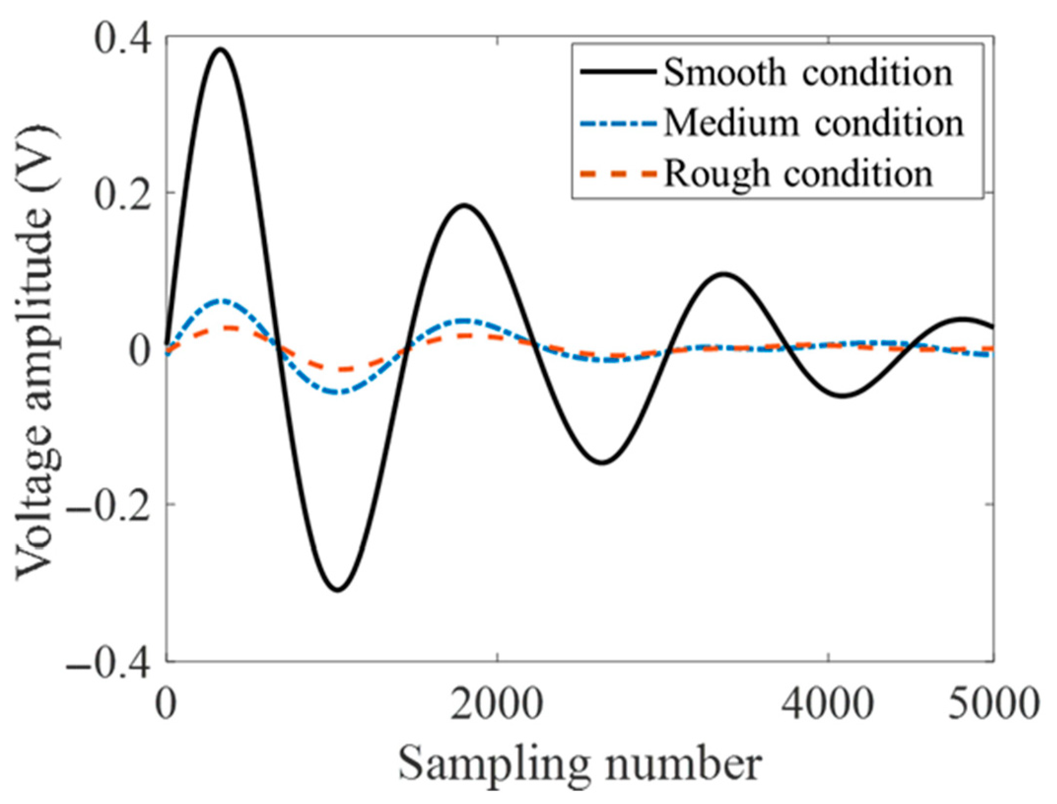
3. Porosity Evaluation in Rough Surface Conditions
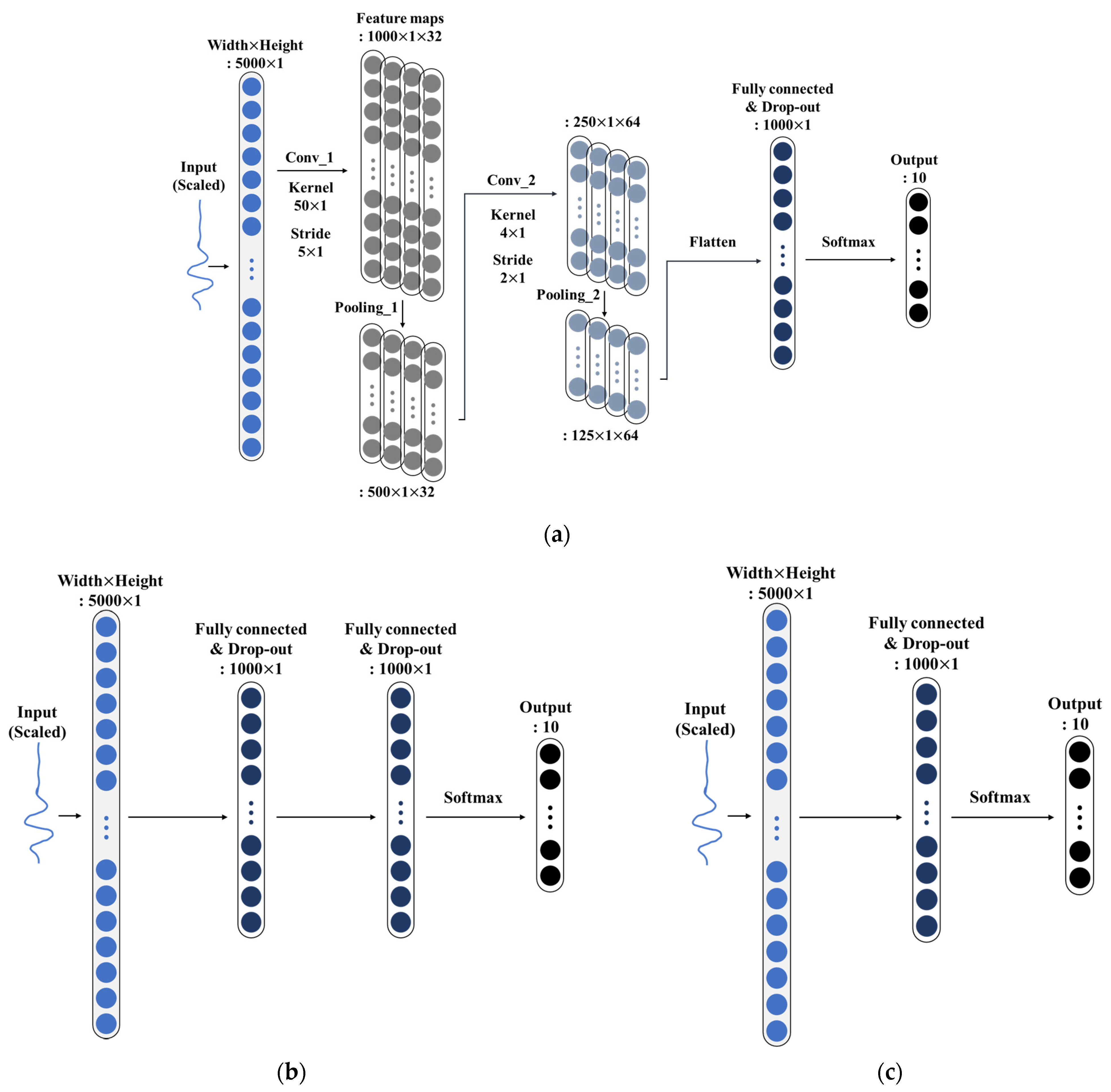
3.1. Structures of Deep Learning Models
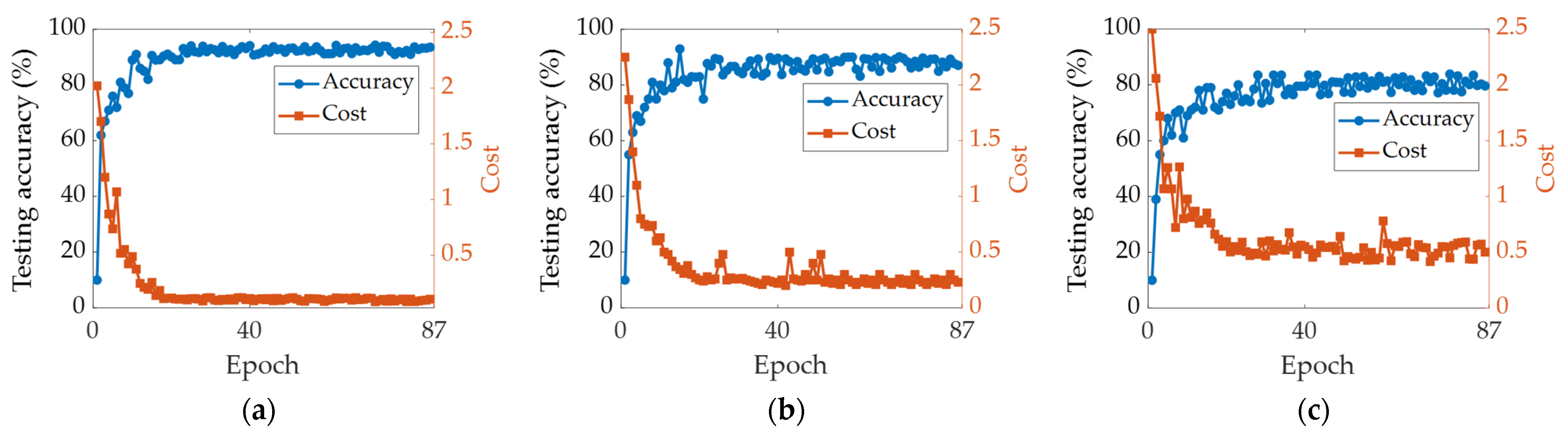
3.2. Procedures to Train and Test the Models
3.3. Evaluation of the Generalization Performance
4. Conclusions
- (1)
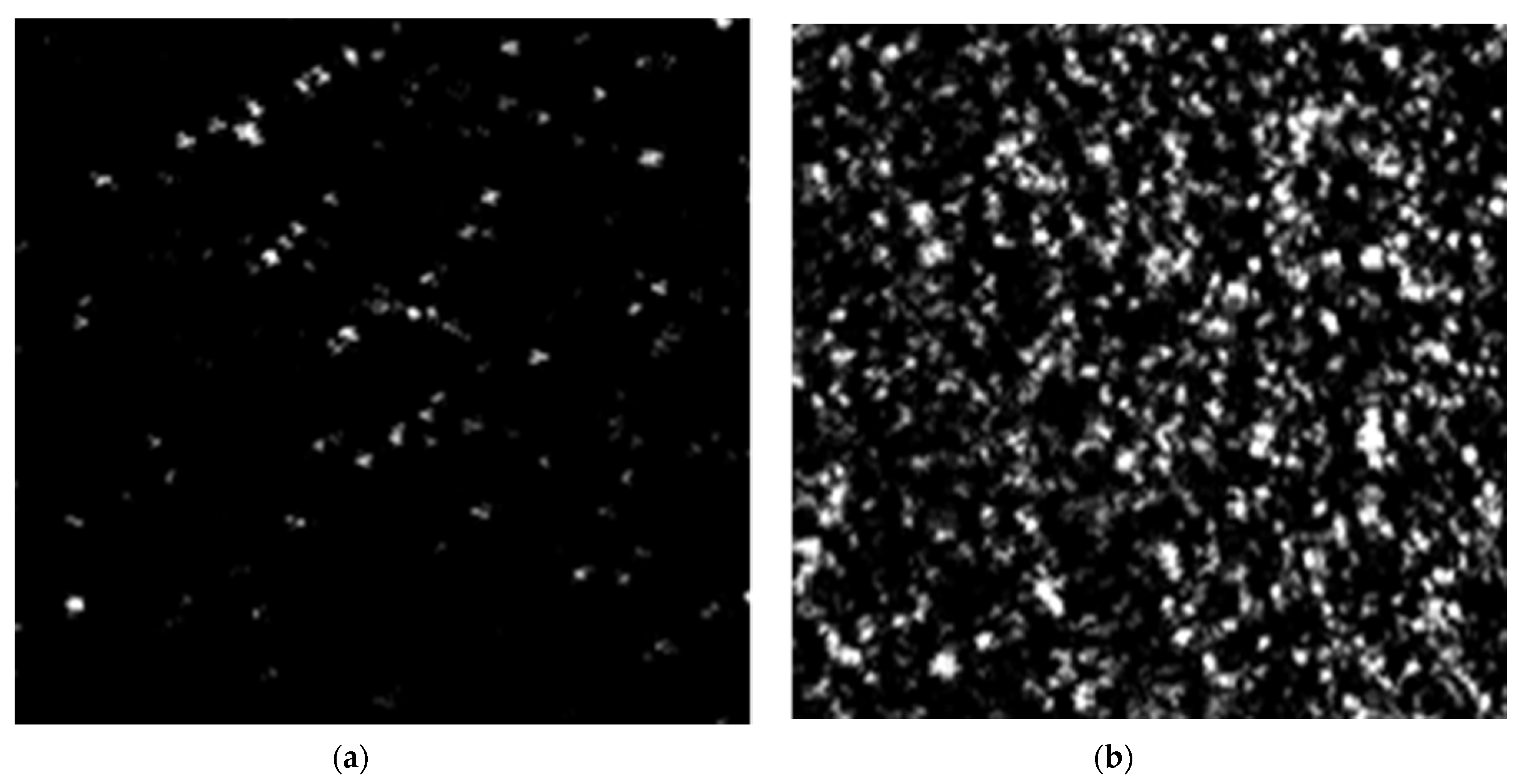
- Various porosity mechanisms were investigated through SAM and OM analysis. Porosity contents increased in the order of normal (the relative porosity content measured by SAM: 0.7%), over-melting (4.2%), LOF (16.1%), and over-melting with low laser power conditions (34%).
- (2)
- A comparison of the performance results of the various DL models showed that all the models were highly accurate at over 80.5%, even for the as-deposited specimens with surfaces in the “rough condition”. In particular, CNN was the most effective at 94.5%. Owing to the low SNR of the measured ultrasonic signal, conventional UT using ultrasonic velocity and ultrasonic attenuation coefficient measurements could not be used to assess “medium condition” and “rough condition” surfaces.
- (3)
- A generalization test was also conducted using newly as-deposited AM specimens that were not used for training to evaluate the applicability of the pre-trained CNN model. The test results confirmed the model’s high evaluation performance of 90.0%, which corresponded well with the results obtained with SAM.
Author Contributions
Funding
Institutional Review Board Statement
Informed Consent Statement
Conflicts of Interest
Appendix A

| CNN | ||||||||||
|---|---|---|---|---|---|---|---|---|---|---|
| Smooth condition | ||||||||||
| (Unit: %) | Lev. 1 | Lev. 2 | Lev. 3 | Lev. 4 | Lev. 5 | Lev. 6 | Lev. 7 | Lev. 8 | Lev. 9 | Lev. 10 |
| Lev. 1 | 90 | 10 | 0 | 0 | 0 | 0 | 0 | 0 | 0 | 0 |
| Lev. 2 | 5 | 95 | 0 | 0 | 0 | 0 | 0 | 0 | 0 | 0 |
| Lev. 3 | 0 | 0 | 100 | 0 | 0 | 0 | 0 | 0 | 0 | 0 |
| Lev. 4 | 0 | 0 | 0 | 100 | 0 | 0 | 0 | 0 | 0 | 0 |
| Lev. 5 | 0 | 0 | 0 | 0 | 100 | 0 | 0 | 0 | 0 | 0 |
| Lev. 6 | 0 | 0 | 0 | 0 | 0 | 100 | 0 | 0 | 0 | 0 |
| Lev. 7 | 0 | 0 | 0 | 0 | 0 | 0 | 100 | 0 | 0 | 0 |
| Lev. 8 | 0 | 0 | 0 | 0 | 0 | 0 | 0 | 100 | 0 | 0 |
| Lev. 9 | 0 | 0 | 0 | 0 | 0 | 0 | 0 | 0 | 100 | 0 |
| Lev. 10 | 0 | 0 | 0 | 0 | 0 | 0 | 0 | 0 | 0 | 100 |
| Medium condition | ||||||||||
| (Unit: %) | Lev. 1 | Lev. 2 | Lev. 3 | Lev. 4 | Lev. 5 | Lev. 6 | Lev. 7 | Lev. 8 | Lev. 9 | Lev. 10 |
| Lev. 1 | 85 | 10 | 0 | 5 | 0 | 0 | 0 | 0 | 0 | 0 |
| Lev. 2 | 10 | 90 | 0 | 0 | 0 | 0 | 0 | 0 | 0 | 0 |
| Lev. 3 | 0 | 0 | 100 | 0 | 0 | 0 | 0 | 0 | 0 | 0 |
| Lev. 4 | 0 | 0 | 0 | 100 | 0 | 0 | 0 | 0 | 0 | 0 |
| Lev. 5 | 0 | 0 | 0 | 0 | 100 | 0 | 0 | 0 | 0 | 0 |
| Lev. 6 | 0 | 0 | 0 | 0 | 0 | 100 | 0 | 0 | 0 | 0 |
| Lev. 7 | 0 | 0 | 0 | 0 | 0 | 0 | 100 | 0 | 0 | 0 |
| Lev. 8 | 0 | 0 | 0 | 0 | 0 | 0 | 0 | 100 | 0 | 0 |
| Lev. 9 | 0 | 0 | 0 | 0 | 0 | 0 | 0 | 0 | 100 | 0 |
| Lev. 10 | 0 | 0 | 0 | 0 | 0 | 0 | 0 | 0 | 0 | 100 |
| Rough condition | ||||||||||
| (Unit: %) | Lev. 1 | Lev. 2 | Lev. 3 | Lev. 4 | Lev. 5 | Lev. 6 | Lev. 7 | Lev. 8 | Lev. 9 | Lev. 10 |
| Lev. 1 | 75 | 20 | 0 | 5 | 0 | 0 | 0 | 0 | 0 | 0 |
| Lev. 2 | 10 | 85 | 5 | 0 | 0 | 0 | 0 | 0 | 0 | 0 |
| Lev. 3 | 5 | 0 | 90 | 5 | 0 | 0 | 0 | 0 | 0 | 0 |
| Lev. 4 | 0 | 0 | 0 | 100 | 0 | 0 | 0 | 0 | 0 | 0 |
| Lev. 5 | 0 | 0 | 0 | 5 | 95 | 0 | 0 | 0 | 0 | 0 |
| Lev. 6 | 0 | 0 | 0 | 0 | 0 | 100 | 0 | 0 | 0 | 0 |
| Lev. 7 | 0 | 0 | 0 | 0 | 0 | 0 | 100 | 0 | 0 | 0 |
| Lev. 8 | 0 | 0 | 0 | 0 | 0 | 0 | 0 | 100 | 0 | 0 |
| Lev. 9 | 0 | 0 | 0 | 0 | 0 | 0 | 0 | 0 | 100 | 0 |
| Lev. 10 | 0 | 0 | 0 | 0 | 0 | 0 | 0 | 0 | 0 | 100 |
| DNN | ||||||||||
|---|---|---|---|---|---|---|---|---|---|---|
| Smooth condition | ||||||||||
| (Unit: %) | Lev. 1 | Lev. 2 | Lev. 3 | Lev. 4 | Lev. 5 | Lev. 6 | Lev. 7 | Lev. 8 | Lev. 9 | Lev. 10 |
| Lev. 1 | 95 | 5 | 0 | 0 | 0 | 0 | 0 | 0 | 0 | 0 |
| Lev. 2 | 5 | 95 | 0 | 0 | 0 | 0 | 0 | 0 | 0 | 0 |
| Lev. 3 | 0 | 0 | 100 | 0 | 0 | 0 | 0 | 0 | 0 | 0 |
| Lev. 4 | 0 | 0 | 0 | 100 | 0 | 0 | 0 | 0 | 0 | 0 |
| Lev. 5 | 0 | 0 | 0 | 5 | 95 | 0 | 0 | 0 | 0 | 0 |
| Lev. 6 | 0 | 0 | 0 | 0 | 0 | 100 | 0 | 0 | 0 | 0 |
| Lev. 7 | 0 | 0 | 0 | 0 | 0 | 0 | 100 | 0 | 0 | 0 |
| Lev. 8 | 0 | 0 | 0 | 0 | 0 | 0 | 0 | 95 | 5 | 0 |
| Lev. 9 | 0 | 0 | 0 | 0 | 0 | 0 | 0 | 0 | 100 | 0 |
| Lev. 10 | 0 | 0 | 0 | 0 | 0 | 0 | 0 | 0 | 0 | 100 |
| Medium condition | ||||||||||
| (Unit: %) | Lev. 1 | Lev. 2 | Lev. 3 | Lev. 4 | Lev. 5 | Lev. 6 | Lev. 7 | Lev. 8 | Lev. 9 | Lev. 10 |
| Lev. 1 | 90 | 10 | 0 | 0 | 0 | 0 | 0 | 0 | 0 | 0 |
| Lev. 2 | 10 | 90 | 0 | 0 | 0 | 0 | 0 | 0 | 0 | 0 |
| Lev. 3 | 0 | 0 | 95 | 5 | 0 | 0 | 0 | 0 | 0 | 0 |
| Lev. 4 | 5 | 0 | 0 | 95 | 0 | 0 | 0 | 0 | 0 | 0 |
| Lev. 5 | 0 | 0 | 0 | 5 | 95 | 0 | 0 | 0 | 0 | 0 |
| Lev. 6 | 0 | 0 | 0 | 0 | 0 | 100 | 0 | 0 | 0 | 0 |
| Lev. 7 | 0 | 0 | 0 | 0 | 0 | 0 | 100 | 0 | 0 | 0 |
| Lev. 8 | 0 | 0 | 0 | 0 | 0 | 0 | 0 | 95 | 0 | 5 |
| Lev. 9 | 0 | 0 | 0 | 0 | 0 | 0 | 0 | 0 | 95 | 5 |
| Lev. 10 | 0 | 0 | 0 | 0 | 0 | 0 | 0 | 0 | 0 | 100 |
| Rough condition | ||||||||||
| (Unit: %) | Lev. 1 | Lev. 2 | Lev. 3 | Lev. 4 | Lev. 5 | Lev. 6 | Lev. 7 | Lev. 8 | Lev. 9 | Lev. 10 |
| Lev. 1 | 70 | 20 | 5 | 5 | 0 | 0 | 0 | 0 | 0 | 0 |
| Lev. 2 | 15 | 80 | 5 | 0 | 0 | 0 | 0 | 0 | 0 | 0 |
| Lev. 3 | 5 | 0 | 90 | 5 | 0 | 0 | 0 | 0 | 0 | 0 |
| Lev. 4 | 10 | 0 | 5 | 85 | 0 | 0 | 0 | 0 | 0 | 0 |
| Lev. 5 | 0 | 0 | 0 | 10 | 90 | 0 | 0 | 0 | 0 | 0 |
| Lev. 6 | 0 | 0 | 0 | 0 | 5 | 95 | 0 | 0 | 0 | 0 |
| Lev. 7 | 0 | 0 | 0 | 0 | 0 | 0 | 100 | 0 | 0 | 0 |
| Lev. 8 | 0 | 0 | 0 | 0 | 0 | 0 | 0 | 95 | 0 | 5 |
| Lev. 9 | 0 | 0 | 0 | 0 | 0 | 0 | 0 | 0 | 90 | 10 |
| Lev. 10 | 0 | 0 | 0 | 0 | 0 | 0 | 0 | 0 | 0 | 100 |
| MLP | ||||||||||
|---|---|---|---|---|---|---|---|---|---|---|
| Smooth condition | ||||||||||
| (Unit: %) | Lev. 1 | Lev. 2 | Lev. 3 | Lev. 4 | Lev. 5 | Lev. 6 | Lev. 7 | Lev. 8 | Lev. 9 | Lev. 10 |
| Lev. 1 | 85 | 15 | 0 | 0 | 0 | 0 | 0 | 0 | 0 | 0 |
| Lev. 2 | 5 | 90 | 0 | 5 | 0 | 0 | 0 | 0 | 0 | 0 |
| Lev. 3 | 5 | 0 | 95 | 0 | 0 | 0 | 0 | 0 | 0 | 0 |
| Lev. 4 | 0 | 0 | 0 | 95 | 0 | 0 | 5 | 0 | 0 | 0 |
| Lev. 5 | 0 | 0 | 0 | 0 | 100 | 0 | 0 | 0 | 0 | 0 |
| Lev. 6 | 0 | 0 | 0 | 0 | 0 | 100 | 0 | 0 | 0 | 0 |
| Lev. 7 | 0 | 0 | 0 | 0 | 0 | 0 | 100 | 0 | 0 | 0 |
| Lev. 8 | 0 | 0 | 0 | 0 | 0 | 0 | 0 | 100 | 0 | 0 |
| Lev. 9 | 0 | 0 | 0 | 0 | 0 | 0 | 0 | 0 | 100 | 0 |
| Lev. 10 | 0 | 0 | 0 | 0 | 0 | 0 | 0 | 0 | 5 | 95 |
| Medium condition | ||||||||||
| (Unit: %) | Lev. 1 | Lev. 2 | Lev. 3 | Lev. 4 | Lev. 5 | Lev. 6 | Lev. 7 | Lev. 8 | Lev. 9 | Lev. 10 |
| Lev. 1 | 80 | 15 | 5 | 0 | 0 | 0 | 0 | 0 | 0 | 0 |
| Lev. 2 | 15 | 80 | 0 | 5 | 0 | 0 | 0 | 0 | 0 | 0 |
| Lev. 3 | 5 | 0 | 90 | 5 | 0 | 0 | 0 | 0 | 0 | 0 |
| Lev. 4 | 0 | 0 | 0 | 95 | 0 | 0 | 5 | 0 | 0 | 0 |
| Lev. 5 | 0 | 0 | 0 | 5 | 95 | 0 | 0 | 0 | 0 | 0 |
| Lev. 6 | 0 | 0 | 0 | 0 | 0 | 100 | 0 | 0 | 0 | 0 |
| Lev. 7 | 0 | 0 | 0 | 0 | 0 | 0 | 95 | 0 | 0 | 5 |
| Lev. 8 | 0 | 0 | 0 | 0 | 0 | 0 | 0 | 95 | 0 | 5 |
| Lev. 9 | 0 | 0 | 0 | 0 | 0 | 0 | 0 | 0 | 100 | 0 |
| Lev. 10 | 0 | 0 | 0 | 0 | 0 | 0 | 5 | 0 | 5 | 90 |
| Rough condition | ||||||||||
| (Unit: %) | Lev. 1 | Lev. 2 | Lev. 3 | Lev. 4 | Lev. 5 | Lev. 6 | Lev. 7 | Lev. 8 | Lev. 9 | Lev. 10 |
| Lev. 1 | 60 | 25 | 5 | 10 | 0 | 0 | 0 | 0 | 0 | 0 |
| Lev. 2 | 15 | 70 | 5 | 5 | 0 | 0 | 5 | 0 | 0 | 0 |
| Lev. 3 | 5 | 0 | 85 | 10 | 0 | 0 | 0 | 0 | 0 | 0 |
| Lev. 4 | 10 | 0 | 10 | 75 | 0 | 0 | 5 | 0 | 0 | 0 |
| Lev. 5 | 0 | 0 | 0 | 10 | 85 | 5 | 0 | 0 | 0 | 0 |
| Lev. 6 | 0 | 0 | 0 | 5 | 5 | 85 | 5 | 0 | 0 | 0 |
| Lev. 7 | 0 | 0 | 0 | 0 | 0 | 0 | 95 | 0 | 0 | 5 |
| Lev. 8 | 0 | 0 | 0 | 0 | 0 | 0 | 0 | 90 | 0 | 10 |
| Lev. 9 | 0 | 0 | 0 | 0 | 0 | 5 | 0 | 0 | 80 | 15 |
| Lev. 10 | 0 | 0 | 0 | 0 | 0 | 0 | 5 | 0 | 15 | 80 |
References
- Gorsse, S.; Hutchinson, C.; Gouné, M.; Banerjee, R. Additive manufacturing of metals: A brief review of the characteristic microstructures and properties of steels, Ti-6Al-4V and high-entropy alloys. Sci. Technol. Adv. Mater. 2017, 18, 584–610. [Google Scholar] [CrossRef] [PubMed]
- Seifi, M.; Salem, A.; Beuth, J.; Harrysson, O.; Lewandowski, J.J. Overview of Materials Qualification Needs for Metal Additive Manufacturing. JOM 2016, 68, 747–764. [Google Scholar] [CrossRef]
- Everton, S.K.; Hirsch, M.; Stravroulakis, P.; Leach, R.K.; Clare, A.T. Review of in-situ process monitoring and in-situ metrology for metal additive manufacturing. Mater. Des. 2016, 95, 431–445. [Google Scholar] [CrossRef]
- Babu, B.; Lundbäck, A.; Lindgren, L.-E. Simulation of Ti-6Al-4V Additive Manufacturing Using Coupled Physically Based Flow Stress and Metallurgical Model. Materials 2019, 12, 3844. [Google Scholar] [CrossRef]
- Wang, Z.; Palmer, T.A.; Beese, A.M. Effect of processing parameters on microstructure and tensile properties of austenitic stainless steel 304L made by directed energy deposition additive manufacturing. Acta Mater. 2016, 110, 226–235. [Google Scholar] [CrossRef]
- Collins, P.C.; Brice, D.A.; Samimi, P.; Ghamarian, I.; Fraser, H.L. Microstructural Control of Additively Manufactured Metallic Materials. Annu. Rev. Mater. Res. 2016, 46, 63–91. [Google Scholar] [CrossRef]
- Yang, K.; Xie, H.; Sun, C.; Zhao, X.; Li, F. Influence of Vanadium on the Microstructure of IN718 Alloy by Laser Cladding. Materials 2019, 12, 3839. [Google Scholar] [CrossRef]
- Everton, S.; Dickens, P.; Tuck, C.; Dutton, B. Evaluation of laser ultrasonic testing for inspection of metal additive manufacturing. Laser 3D Manuf. II Int. Soc. Opt. Photonics 2015, 9353, 935316. [Google Scholar] [CrossRef]
- Clark, D.; Sharples, S.D.; Wright, D.C. Development of online inspection for additive manufacturing products. Insight 2011, 53, 610–613. [Google Scholar] [CrossRef]
- Eren, E.; Kurama, S.; Solodov, I. Characterization of porosity and defect imaging in ceramic tile using ultrasonic inspections. Ceram. Int. 2012, 38, 2145–2151. [Google Scholar] [CrossRef]
- Honarvar, F.; Varvani-Farahani, A. A review of ultrasonic testing applications in additive manufacturing: Defect evaluation, material characterization, and process control. Ultrasonics 2020, 108, 106227. [Google Scholar] [CrossRef]
- Chabot, A.; Laroche, N.; Carcreff, E.; Rauch, M.; Hascoët, J.-Y. Towards defect monitoring for metallic additive manufacturing components using phased array ultrasonic testing. J. Intell. Manuf. 2019, 31, 1191–1201. [Google Scholar] [CrossRef]
- Jeong, H.; Hsu, D.K. Experimental analysis of porosity-induced ultrasonic attenuation and velocity change in carbon composites. Ultrasonics 1995, 33, 195–203. [Google Scholar] [CrossRef]
- Park, S.-H.; Kim, J.; Jhang, K.-Y. Relative measurement of the acoustic nonlinearity parameter using laser detection of an ultrasonic wave. Int. J. Precis. Eng. Manuf. 2017, 18, 1347–1352. [Google Scholar] [CrossRef]
- Jeong, H. Effects of Voids on the Mechanical Strength and Ultrasonic Attenuation of Laminated Composites. J. Compos. Mater. 1997, 31, 276–292. [Google Scholar] [CrossRef]
- Kim, H.S.; Bush, M.B. The effects of grain size and porosity on the elastic modulus of nanocrystalline materials. Nanostruct. Mater. 1999, 11, 361–367. [Google Scholar] [CrossRef]
- Birt, E.A.; Smith, R.A. A review of NDE methods for porosity measurement in fibre-reinforced polymer composites. Insight 2004, 46, 681–686. [Google Scholar] [CrossRef]
- Hernandez, M.G.; Izquierdo, M.A.G.; Ibanez, A.; Anaya, J.J.; Ullate, L.G. Porosity estimation of concrete by ultrasonic NDE. Ultrasonics 2000, 38, 531–533. [Google Scholar] [CrossRef]
- Slotwinski, J.A.; Garboczi, E.J.; Hebenstreit, K.M. Porosity Measurements and Analysis for Metal Additive Manufacturing Process Control. J. Res. Natl. Inst. Stand. Technol. 2014, 119, 494–528. [Google Scholar] [CrossRef]
- Karthik, N.V.; Gu, H.; Pal, D.; Starr, T.; Stucker, B. High frequency ultrasonic non destructive evaluation of additively manufactured components. In Proceedings of the 24th International Solid Freeform Fabrication Symposium, Austin, TX, USA, 12–14 August 2013; pp. 311–325. [Google Scholar]
- Javidrad, H.R.; Salemi, S. Determination of elastic constants of additive manufactured Inconel 625 specimens using an ultrasonic technique. Int. J. Adv. Manuf. Technol. 2020, 107, 4597–4607. [Google Scholar] [CrossRef]
- Bakre, C.; Hassanian, M.; Lissenden, C. Influence of surface roughness from additive manufacturing on laser ultrasonics measurements. In AIP Conference Proceedings; AIP Publishing LLC: Melville, NY, USA, 2019; p. 020009. [Google Scholar]
- Calignano, F.; Manfredi, D.; Ambrosio, E.P.; Iuliano, L.; Fino, P. Influence of process parameters on surface roughness of aluminum parts produced by DMLS. Int. J. Adv. Manuf. Technol. 2013, 67, 2743–2751. [Google Scholar] [CrossRef]
- Tyagi, P.; Goulet, T.; Riso, C.; Stephenson, R.; Chuenprateep, N.; Schlitzer, J.; Benton, C.; Garcia-Moreno, F. Reducing the roughness of internal surface of an additive manufacturing produced 316 steel component by chempolishing and electropolishing. Addit. Manuf. 2019, 25, 32–38. [Google Scholar] [CrossRef]
- Whip, B.; Sheridan, L.; Gockel, J. The effect of primary processing parameters on surface roughness in laser powder bed additive manufacturing. Int. J. Adv. Manuf. Technol. 2019, 103, 4411–4422. [Google Scholar] [CrossRef]
- Richardson, F.; Reynolds, D.; Dehak, N. Deep Neural Network Approaches to Speaker and Language Recognition. IEEE Signal Process. Lett. 2015, 22, 1671–1675. [Google Scholar] [CrossRef]
- Noda, K.; Yamaguchi, Y.; Nakadai, K.; Okuno, H.G.; Ogata, T. Audio-visual speech recognition using deep learning. Appl. Intell. 2015, 42, 722–737. [Google Scholar] [CrossRef]
- Hamel, P.; Eck, D. Learning features from music audio with deep belief networks. ISMIR 2010, 10, 339–344. [Google Scholar]
- Kim, Y.; Lee, H.; Provost, E.M. Deep learning for robust feature generation in audiovisual emotion recognition. In Proceedings of the IEEE International Conference on Acoustics, Speech and Signal Processing, Vancouver, BC, Canada, 26–31 May 2013; pp. 3687–3691. [Google Scholar]
- Hou, W.; Wei, Y.; Guo, J.; Jin, Y.; Zhu, C. Automatic Detection of Welding Defects using Deep Neural Network. J. Phys. Conf. Ser. 2018, 933, 012006. [Google Scholar] [CrossRef]
- Meng, M.; Chua, Y.J.; Wouterson, E.; Ong, C.P.K. Ultrasonic signal classification and imaging system for composite materials via deep convolutional neural networks. Neurocomputing 2017, 257, 128–135. [Google Scholar] [CrossRef]
- Zhu, P.; Cheng, Y.; Banerjee, P.; Tamburrino, A.; Deng, Y. A novel machine learning model for eddy current testing with uncertainty. NDT E Int. 2019, 101, 104–112. [Google Scholar] [CrossRef]
- Aldrin, J.C.; Forsyth, D.S. Demonstration of using signal feature extraction and deep learning neural networks with ultrasonic data for detecting challenging discontinuities in composite panels. AIP Conf. Proc. 2019, 2102, 020012. [Google Scholar]
- Munir, N.; Kim, H.-J.; Park, J.; Song, S.-J.; Kang, S.-S. Convolutional neural network for ultrasonic weldment flaw classification in noisy conditions. Ultrasonics 2019, 94, 74–81. [Google Scholar] [CrossRef] [PubMed]
- Gao, F.; Li, B.; Chen, L.; Wei, X.; Shang, Z.; He, C. Ultrasonic signal denoising based on autoencoder. Rev. Sci. Instrum. 2020, 91, 045104. [Google Scholar] [CrossRef] [PubMed]
- Margrave, F.; Rigas, K.; Bradley, D.; Barrowcliffe, P. The use of neural networks in ultrasonic flaw detection. Measurement 1999, 25, 143–154. [Google Scholar] [CrossRef]
- Yuan, S.; Wang, L.; Peng, G. Neural network method based on a new damage signature for structural health monitoring. Thin-Walled Struct. 2005, 43, 553–563. [Google Scholar] [CrossRef]
- Fahad, M.; Kamal, K.; Zafar, T.; Qayyum, R.; Tariq, S.; Khan, K. Corrosion detection in industrial pipes using guided acoustics and radial basis function neural network. In Proceedings of the 2017 International Conference on Robotics and Automation Sciences (ICRAS), Hong Kong, China, 26–29 August 2017; pp. 129–133. [Google Scholar]
- Cai, W.; Wang, J.; Zhou, Q.; Yang, Y.; Jiang, P. Equipment and Machine Learning in Welding Monitoring: A Short Review. In Proceedings of the 5th International Conference on Mechatronics and Robotics Engineering, Rome, Italy, 16–19 February 2019; pp. 9–15. [Google Scholar]
- Wang, Y.; Shi, F.; Tong, X. A Welding Defect Identification Approach in X-ray Images Based on Deep Convolutional Neural Networks. In Proceedings of the International Conference on Intelligent Computing, Nanchang, China, 3–6 August 2019; pp. 953–964. [Google Scholar]
- Isamail, L.; Maskuri, N.L.; Isip, N.J.; Lokman, S.F.; Abu Bakar, M.H. Deep Neural Network Modeling for Metallic Component Defects Using the Finite Element Model. In Progress in Engineering Technology; Springer: Cham, Switzerland, 2019; pp. 259–270. [Google Scholar]
- Zhang, W.; Li, C.; Peng, G.; Chen, Y.; Zhang, Z. A deep convolutional neural network with new training methods for bearing fault diagnosis under noisy environment and different working load. Mech. Syst. Signal Process. 2018, 100, 439–453. [Google Scholar] [CrossRef]
- Grasso, M.; Colosimo, B.M. Process defects and in situ monitoring methods in metal powder bed fusion: A review. Meas. Sci. Technol. 2017, 28, 044005. [Google Scholar] [CrossRef]
- Qi, T.; Zhu, H.; Zhang, H.; Yin, J.; Ke, L.; Zeng, X. Selective laser melting of Al7050 powder: Melting mode transition and comparison of the characteristics between the keyhole and conduction mode. Mater. Des. 2017, 135, 257–266. [Google Scholar] [CrossRef]
- Guo, Q.; Zhao, C.; Qu, M.; Xiong, L.; Escano, L.I.; Hojjatzadeh, S.M.H.; Parab, N.D.; Fezzaa, K.; Everhart, W.; Sun, T.; et al. In-situ characterization and quantification of melt pool variation under constant input energy density in laser powder bed fusion additive manufacturing process. Addit. Manuf. 2019, 28, 600–609. [Google Scholar] [CrossRef]
- Leung, C.L.A.; Marussi, S.; Atwood, R.C.; Towrie, M.; Withers, P.J.; Lee, P.D. In situ X-ray imaging of defect and molten pool dynamics in laser additive manufacturing. Nat. Commun. 2018, 9, 1355. [Google Scholar] [CrossRef]
- Jung, K.-H.; Kim, D.-H.; Kim, H.-J.; Park, S.-H.; Jhang, K.-Y.; Kim, H.-S. Finite element analysis of a low-velocity impact test for glass fiber-reinforced polypropylene composites considering mixed-mode interlaminar fracture toughness. Compos. Struct. 2017, 160, 446–456. [Google Scholar] [CrossRef]
- Ziółkowski, G.; Chlebus, E.; Szymczyk, P.; Kurzac, J. Application of X-ray CT method for discontinuity and porosity detection in 316L stainless steel parts produced with SLM technology. Arch. Civ. Mech. Eng. 2014, 14, 608–614. [Google Scholar] [CrossRef]
- Koester, L.W.; Taheri, H.; Bigelow, T.A.; Collins, P.C.; Bonds, L.J. Nondestructive Testing for Metal Parts Fabricated Using Powder-Based Additive Manufacturing. Mater. Eval. 2018, 76, 514–524. [Google Scholar]
- Jhang, K.-Y.; Choi, S.; Kim, J. Measurement of Nonlinear Ultrasonic Parameters from Higher Harmonics. In Measurement of Nonlinear Ultrasonic Characteristics; Springer: Singapore, 2020; pp. 9–60. [Google Scholar]
- LeCun, Y.; Bengio, Y.; Hinton, G. Deep learning. Nature 2015, 521, 436–444. [Google Scholar] [CrossRef]
- Hinton, G.E.; Osindero, S.; Teh, Y.-W. A Fast Learning Algorithm for Deep Belief Nets. Neural Comput. 2006, 18, 1527–1554. [Google Scholar] [CrossRef] [PubMed]
- Sambath, S.; Nagaraj, P.; Selvakumar, N.; Arunachalam, S.; Page, T. Automatic detection of defects in ultrasonic testing using artificial neural network. Int. J. Microstruct. Mater. Prop. 2010, 5, 561. [Google Scholar] [CrossRef]
- LeCun, Y.; Bengio, Y. Convolutional Networks for Images, Speech, and Time-Series. Handb. Brain Theory Neural Netw. 1995, 3361, 1995. [Google Scholar]
- Aghdam, H.H.; Heravi, E.J. Guide to Convolutional Neural Networks; Springer: New York, NY, USA, 2017; Volume 10, pp. 973–978. [Google Scholar]
- Wang, W.; Zhu, M.; Wang, J.; Zeng, X.; Yang, Z. End-to-end encrypted traffic classification with one-dimensional convolution neural networks. In Proceedings of the IEEE International Conference on Intelligence and Security Informatics (ISI), Beijing, China, 22–24 July 2017; pp. 43–48. [Google Scholar] [CrossRef]
- Dahl, G.E.; Sainath, T.N.; Hinton, G.E. Improving deep neural networks for LVCSR using rectified linear units and dropout. In Proceedings of the 2013 IEEE International Conference on Acoustics, Speech and Signal Processing, Vancouver, BC, Canada, 26–31 May 2013; pp. 8609–8613. [Google Scholar]
- Srivastava, N.; Hinton, G.; Krizhevsky, A.; Sutskever, I.; Salakhutdinov, R. Dropout: A simple way to prevent neural networks from overfitting. J. Mach. Learn. Res. 2014, 15, 1929–1958. [Google Scholar]
- Zhang, C.; Bengio, S.; Hardt, M.; Recht, B.; Vinyals, O. Understanding deep learning requires rethinking generalization. arXiv 2016, arXiv:1611.03530. [Google Scholar]


| Specimen Name | #1 | #2 | #3 | #4 | #5 | #6 | #7 | #8 | #9 | #10 |
|---|---|---|---|---|---|---|---|---|---|---|
| Laser power (W) | 275 | 355 | 275 | 235 | 315 | 355 | 355 | 355 | 235 | 235 |
| Scanning speed (mm/s) | 1091 | 1315 | 849 | 1187 | 1458 | 1517 | 1644 | 1793 | 768 | 725 |
| Roughness Condition | Ra Value (μm) | Surface Polishing Method |
|---|---|---|
| Smooth condition | 0.65 | Wire electrical discharge machining |
| Medium condition | 3.1 | Hand grinder |
| Rough condition | 6.4 | X (As-deposited state) |
| Specimen Name | #1 | #2 | #3 | #4 | #5 | #6 | #7 | #8 | #9 | #10 |
|---|---|---|---|---|---|---|---|---|---|---|
| Porosity (%) | 0.7 | 3.2 | 5.2 | 7.6 | 11 | 13 | 23 | 26 | 29 | 39 |
| Porosity Level | Lev. 1 (0–2.5) | Lev. 2 (2.5–5) | Lev. 3 (5–7.5) | Lev. 4 (7.5–10) | Lev. 5 (10–12.5) | Lev. 6 (12.5–15) | Lev. 7 (22.5–25) | Lev. 8 (25–27.5) | Lev. 9 (27.5–30) | Lev. 10 (30-) |
| Model | CNN | DNN | MLP |
|---|---|---|---|
| Input | 5000 | 5000 | 5000 |
| 1st conv: Feature map/Kernel/Stride | 32/50/5 | - | - |
| 1st max-pooling: Kernel/Stride | 2/2 | - | - |
| 2nd conv: Feature map/Kernel/Stride | 64/4/2 | - | - |
| 2nd max-pooling: Kernel/Stride | 2/2 | - | - |
| Fully connected (Wide) | 1000 | 1000 | 1000 |
| Fully connected (Deep) | 1 | 2 | 1 |
| Drop out | 70% | 70% | 70% |
| Learning rate | 0.001 | 0.001 | 0.001 |
| Cost function | Softmax cross-entropy | Softmax cross-entropy | Softmax cross-entropy |
| Activation function | ReLU | ReLU | ReLU |
| Porosity Level | Smooth Condition | Medium Condition | Rough Condition | ||||||
|---|---|---|---|---|---|---|---|---|---|
| Specimen | No. of Signals | Specimen | No. of Signals | Specimen | No. of Signals | ||||
| Train | Test | Train | Test | Train | Test | ||||
| Lev. 1 | #1 | 80 | 20 | #1′ | 80 | 20 | #1′ | 80 | 20 |
| Lev. 2 | #2 | 80 | 20 | #2′ | 80 | 20 | #2′ | 80 | 20 |
| Lev. 3 | #3 | 80 | 20 | #3′ | 80 | 20 | #3′ | 80 | 20 |
| Lev. 4 | #4 | 80 | 20 | #4′ | 80 | 20 | #4′ | 80 | 20 |
| Lev. 5 | #5 | 80 | 20 | #5′ | 80 | 20 | #5′ | 80 | 20 |
| Lev. 6 | #6 | 80 | 20 | #6′ | 80 | 20 | #6′ | 80 | 20 |
| Lev. 7 | #7 | 80 | 20 | #7′ | 80 | 20 | #7′ | 80 | 20 |
| Lev. 8 | #8 | 80 | 20 | #8′ | 80 | 20 | #8′ | 80 | 20 |
| Lev. 9 | #9 | 80 | 20 | #9′ | 80 | 20 | #9′ | 80 | 20 |
| Lev. 10 | #10 | 80 | 20 | #10′ | 80 | 20 | #10′ | 80 | 20 |
| Classification | Testing Performance (%) | ||||||||
|---|---|---|---|---|---|---|---|---|---|
| Smooth Condition | Medium Condition | Rough Condition | |||||||
| CNN | DNN | MLP | CNN | DNN | MLP | CNN | DNN | MLP | |
| Lev. 1 | 90 | 95 | 85 | 85 | 90 | 80 | 75 | 70 | 60 |
| Lev. 2 | 95 | 95 | 90 | 90 | 90 | 80 | 85 | 80 | 70 |
| Lev. 3 | 100 | 100 | 95 | 100 | 95 | 90 | 90 | 90 | 85 |
| Lev. 4 | 100 | 100 | 95 | 100 | 95 | 95 | 100 | 85 | 75 |
| Lev. 5 | 100 | 95 | 100 | 100 | 95 | 95 | 95 | 90 | 85 |
| Lev. 6 | 100 | 100 | 100 | 100 | 100 | 100 | 100 | 95 | 85 |
| Lev. 7 | 100 | 100 | 100 | 100 | 100 | 95 | 100 | 100 | 95 |
| Lev. 8 | 100 | 95 | 100 | 100 | 95 | 95 | 100 | 95 | 90 |
| Lev. 9 | 100 | 100 | 100 | 100 | 95 | 100 | 100 | 90 | 80 |
| Lev. 10 | 100 | 100 | 95 | 100 | 100 | 90 | 100 | 100 | 80 |
| Average | 98.5 | 98 | 96 | 97.5 | 95.5 | 92 | 94.5 | 89.5 | 80.5 |
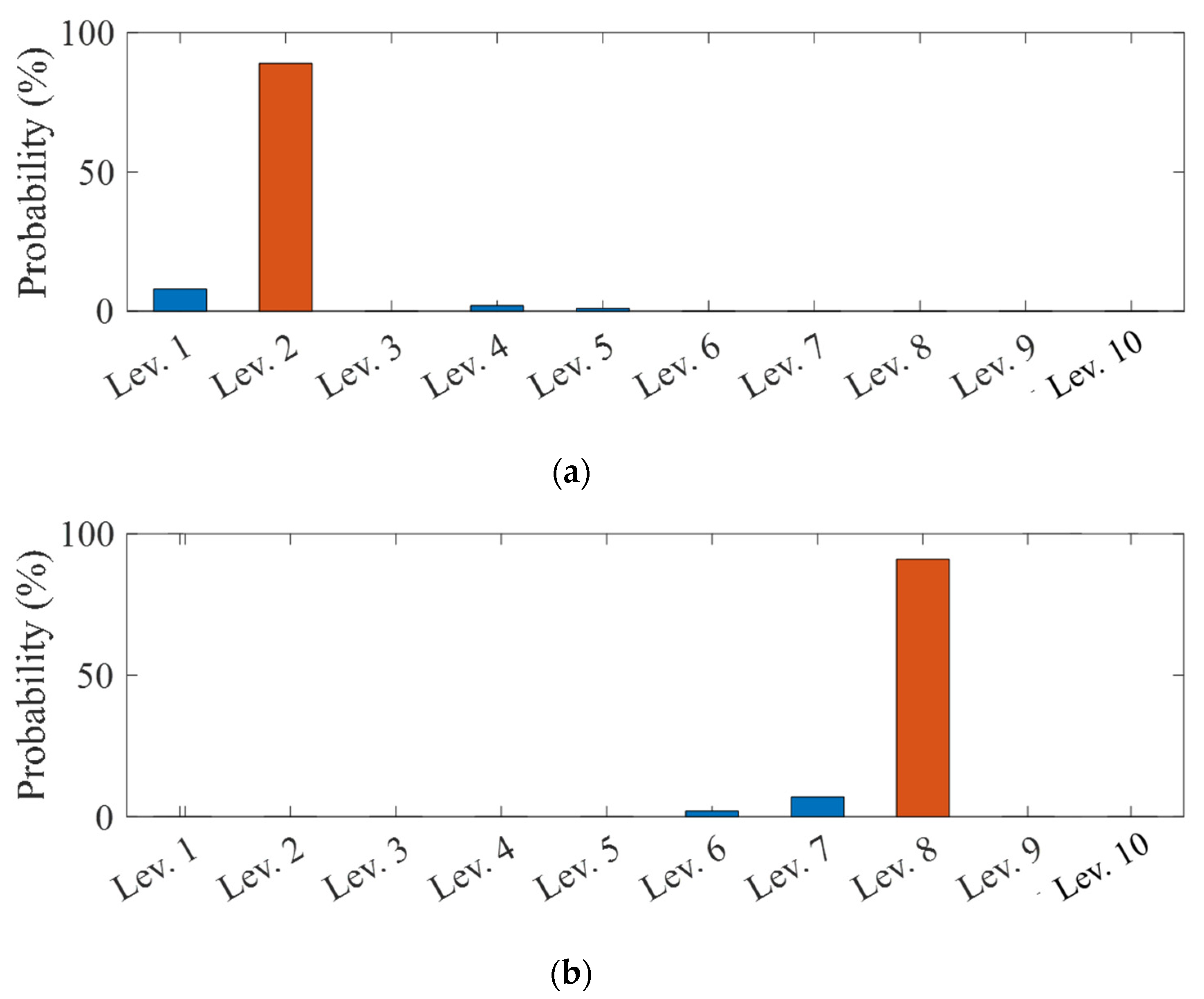
| AM Specimen | Porosity Evaluation Results | ||
|---|---|---|---|
| Pre-Trained Model | SAM | ||
| Porosity Level | Porosity Content (%) | Porosity Content (%) | |
| Test-#1 | Lev. 2 | 2.5–5 | 4.3 |
| Test-#2 | Lev. 8 | 25–27.5 | 27 |
Publisher’s Note: MDPI stays neutral with regard to jurisdictional claims in published maps and institutional affiliations. |
© 2021 by the authors. Licensee MDPI, Basel, Switzerland. This article is an open access article distributed under the terms and conditions of the Creative Commons Attribution (CC BY) license (http://creativecommons.org/licenses/by/4.0/).
Share and Cite
Park, S.-H.; Hong, J.-Y.; Ha, T.; Choi, S.; Jhang, K.-Y. Deep Learning-Based Ultrasonic Testing to Evaluate the Porosity of Additively Manufactured Parts with Rough Surfaces. Metals 2021, 11, 290. https://doi.org/10.3390/met11020290
Park S-H, Hong J-Y, Ha T, Choi S, Jhang K-Y. Deep Learning-Based Ultrasonic Testing to Evaluate the Porosity of Additively Manufactured Parts with Rough Surfaces. Metals. 2021; 11(2):290. https://doi.org/10.3390/met11020290
Chicago/Turabian StylePark, Seong-Hyun, Jung-Yean Hong, Taeho Ha, Sungho Choi, and Kyung-Young Jhang. 2021. "Deep Learning-Based Ultrasonic Testing to Evaluate the Porosity of Additively Manufactured Parts with Rough Surfaces" Metals 11, no. 2: 290. https://doi.org/10.3390/met11020290
APA StylePark, S.-H., Hong, J.-Y., Ha, T., Choi, S., & Jhang, K.-Y. (2021). Deep Learning-Based Ultrasonic Testing to Evaluate the Porosity of Additively Manufactured Parts with Rough Surfaces. Metals, 11(2), 290. https://doi.org/10.3390/met11020290