Experimental Study of the Velocity of the Electrovortex Flow of In-Ga-Sn in Hemispherical Geometry

Abstract

The paper describes the application of the thermocorrelation method for measuring the velocity in a current-carrying liquid. An electrovortex flow occurs when the current passing through a conducting medium interacts with its own magnetic field. Measurements of the velocity of the turbulent electrovortex flow of the liquid metal (eutectic alloy In-Ga-Sn) were carried out in a hemispherical container in the range of currents of 100–450 amperes in the presence and absence of compensation of the Earth’s magnetic field. The efficiency of the thermocorrelation method in a current-carrying liquid has been demonstrated. The dependences of the axial velocity on the current and the velocity profiles along the axis were obtained. It was found that the presence of the Earth’s magnetic field leads to a significant decrease in the average value of the axial velocity in the entire range of currents.

1. Introduction

Currently, due to the increased requirements for the energy efficiency of electrometallurgical plants, there is a steady trend towards an increase in their capacity. In connection with this circumstance, in practice, one has to deal with the enhancement of the influence of various magnetohydrodynamic (MHD) effects and, in particular, the generation of so-called electrovortex flows (EVF) in a current-carrying liquid—a metal melt [1]. The presence of EVF, which are formed as a result of the interaction of an electric current passed through an electrically conductive liquid, with the intrinsic magnetic field (MF) of this current, leads to a radical restructuring of the hydrodynamic structure in the volume of the melting metal. This circumstance significantly affects energy consumption and the quality of products, which determines the paramount importance and relevance of the study of electrovortex flows. The experimental study of electrovortex flows in industrial conditions is very difficult due to the complexity of measuring the velocity in a high-temperature and aggressive liquid metal environment, and the computational methods for studying EVF require additional verification.

Below we give a brief overview of the methods for measuring the velocity in liquid metals (LM) with the justification of their application under certain conditions. All methods for measuring velocity in a LM can be divided into several categories: probe and non-contact, methods that allow to measure average values or pulsation characteristics, and methods that measure average values in space or allow measurements in a small volume of finite size. At the same time, if in laboratory conditions the problem of measuring the velocity in a liquid metal can still be solved relatively successfully due to the use of various model metals and alloys that retain a liquid state at room or low temperatures (mercury, sodium, tin, and various gallium alloys), then in industrial conditions, at temperatures reaching 1000–2000 °C, few workable methods are known.

The Pitot tube is the oldest method for measuring the velocity of liquid media. This method is ineffective due to the high density of liquid metals (except sodium), it allows you to obtain only average values of the velocity and, like any probe method, obstructs the flow; hot-wire anemometer—ineffective in non-isothermal environments and environments with high thermal conductivity, which include liquid metals (nevertheless, there are attempts to use this method in relation to LM [2]; the “Lorentz Force Velocimetry” method [3] based on measuring the force acting with the side of a moving conductive liquid on a permanent magnet, allows you to measure only the space-averaged values of velocity (flow rate); the ultrasonic Doppler anemometer [4] combines the advantages of contactlessness and the ability to measure at a point (measurement occurs along the beam), but, firstly, there are limitations associated with the orientation beam on an installation or industrial unit, and, secondly, this method is extremely demanding on the composition of the alloy—particles (usually oxides) from which ultrasound is reflected, for this reason, UDA is usually used to measure the velocity in gallium alloys, which oxidize well in air and oxide particles fall into the volume of LM; and fiber-optic method [5]—a probe method that allows performing fine measurements (including velocity pulsations) in a small measuring volume (40 × 40 × 500 microns), but having temperature limitations (up to 100 °C).

In our work, we use the thermocorrelation method [6,7] to measure the velocity in an electric vortex flow in a hemispherical container. Apparently, this is the first work where this method is used to measure velocity in a current-carrying fluid. This problem, about the study of the hydrodynamic structure of the flow caused by the spreading of electric current from a point source into a hemispherical volume filled with liquid metal, occupies a special place among the model studies of EVF. This geometry of the working bath has a number of important practical advantages and features, which make it possible to study EVF in its most general form. These features include, first, the existence under these conditions of analytical dependences for the current density and magnetic field. Secondly, this geometry is typical for industrial tasks associated with metal remelting (electroslag welding, and electric arc and electroslag metal remelting). Third, an interesting effect of swirling of an axisymmetric electric vortex flow is observed on the hemispherical model.

The thermal correlation method is a probe method and allows you to measure only the average value of the velocity during a certain specified time interval (in our conditions, the duration is 30–120 s). At the same time, the probe is simple in design and can be used in industrial installations. The use of high-temperature, tungsten–rhenium or platinum–rhodium thermocouples in the probe makes it possible to measure the velocity of liquid metal at temperatures up to 2500 °C. We use the thermocorrelation method in a laboratory setup.

Despite a significant number of studies of EVF, analytical [8], numerical [9], and experimental [10], many questions remain insufficiently studied, which is associated with both the complexity of the object itself and the laboriousness of the measurements.

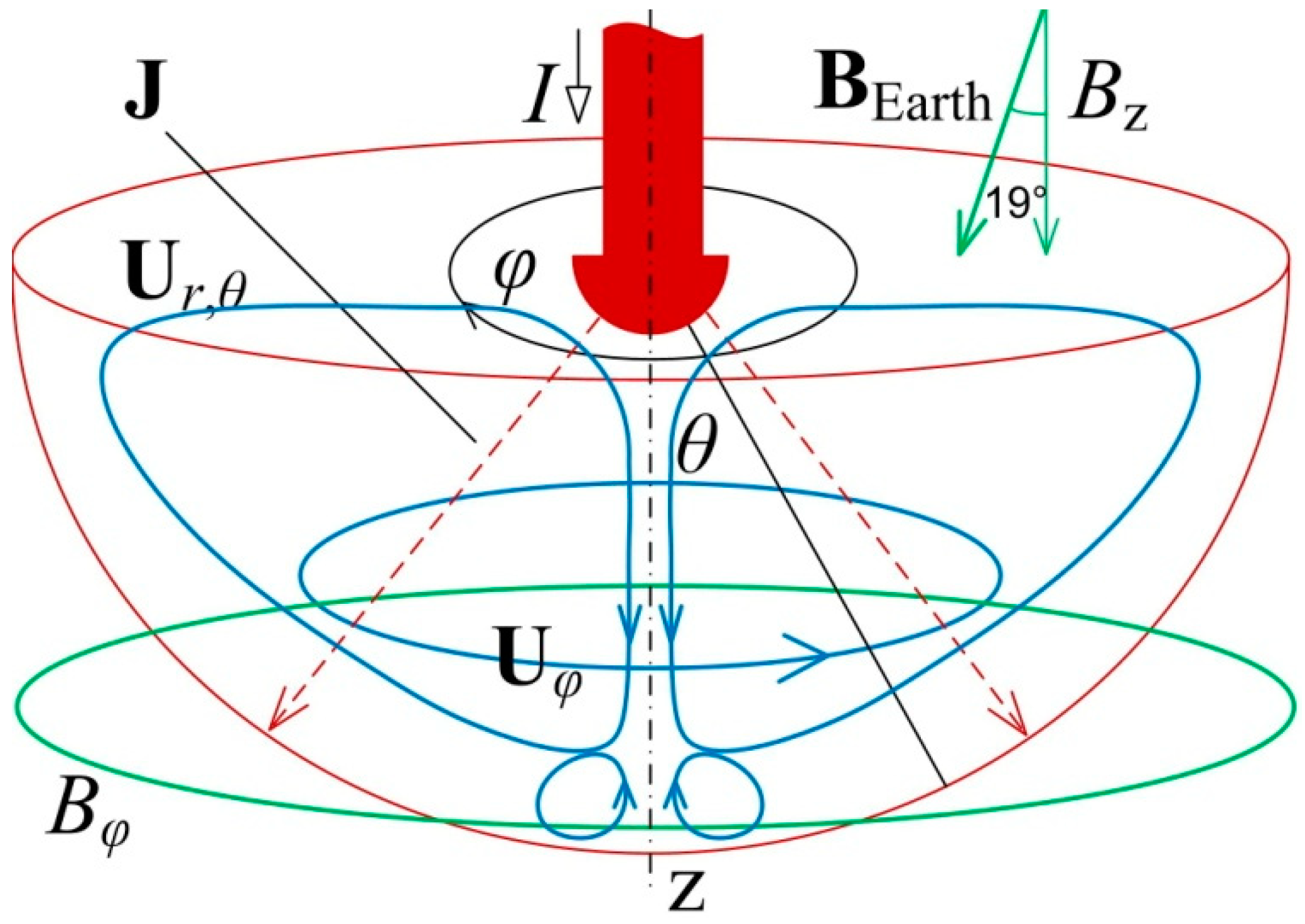
2. Mathematical Description of Processes

As mentioned above, EVF are formed as a result of the interaction of an inhomogeneous electric current of density J with its own magnetic field B (see Figure 1). The Navier–Stokes equation describing the hydrodynamics of an electric vortex flow has the form

$$\rho \left(\frac{\partial U}{\partial \tau }+\left(U\nabla \right)U\right)=-\nabla p+\rho \nu \Delta U+\rho g+F,$$

(1)

where U—velocity, t—time, ρ—density, ν—kinematic viscosity, F = J × B is the electromagnetic force that causes the movement of an electrically conductive fluid.

For a hemispherical geometry, in which the current density J_r depending on the radius r (in the spherical coordinates), changes as

$$J_r=\frac{I}{2\pi r^2},$$

(2)

from Maxwell’s equation

$$\nabla \times B={\mu }_{0}J,$$

(3)

the expression for the distribution of the magnetic field can be easily obtained

$$B_{\phi }=\frac{{\mu }_{0}I\left(1-\cos \theta \right)}{2\pi r\sin \theta }.$$

(4)

Then the expression for the electromagnetic force in a liquid metal has the form

$$F_{\theta }=-\frac{{\mu }_0{I}^2(1-\cos \theta )}{4\pi r^3\sin \theta }.$$

(5)

The system can be characterized by the following dimensionless parameters

$$\mathrm{S}=\frac{{\mu }_0{I}^2}{\rho {\nu }^2},$$

(6)

and this parameter determines the intensity and flow regimes.

At currents > 30 kA (as shown in [11]), or with an external axial field of more than 0.0025 T [12], we must also take into account the currents induced by the motion of the liquid, and then the expression for the current density will have the form

$$J=\sigma \left(E+U\times B\right),$$

(7)

here μ₀—magnetic constant, φ and θ azimuthal and polar angles in the spherical coordinates, σ is the conductivity of the medium, E is the electric field, and, in the general case, it is also necessary to take into account the magnetic fields of the induced currents and to solve the complete magnetohydrodynamic problem including equations for the magnetic field.

A schematic diagram of the formation of the EVF in a hemispherical container is shown in Figure 1. In the absence of external magnetic fields, the magnetic field of an axisymmetric system has only one component of the magnetic field (azimuthal) and, accordingly, one component of the force (poloidal). In a hemisphere, such a force creates a toroidal flow directed downward on the axis.

External magnetic fields interacting with an electric current passing through a liquid metal also create electromagnetic forces, then B = B_own + B_ext, where B_own is the own magnetic field of the current, B_ext is an external magnetic field, for example, the magnetic field of the Earth or current leads.

At the latitude of Moscow, the Earth’s magnetic field has an inclination of 19° and a magnitude of ~52.175 μT (Data of The Pushkov Institute of Terrestrial Magnetism, Ionosphere and Radiowave Propagation of the Russian Academy of Sciences). Thus, the vertical component of the magnetic field is ~49 μT. The vertical component of the magnetic field B_z interacting with the radial component of the current density creates an azimuthal component of the electromagnetic force

$$F_{\phi }=-J_R{B}_z,$$

(8)

For clarity, the expression is given in cylindrical coordinates (here J_R is a radial component of current density), in spherical coordinates, the expression for the force is

$$F_{\phi }=-J_r{B}_z\sin \theta .$$

(9)

In a converging flow, this component creates a significant force and the study of the influence of the Earth’s magnetic field on the EVF swirl is discussed in [13,14,15].

In experiments, the Earth’s magnetic field can only be compensated by an oppositely directed magnetic field.

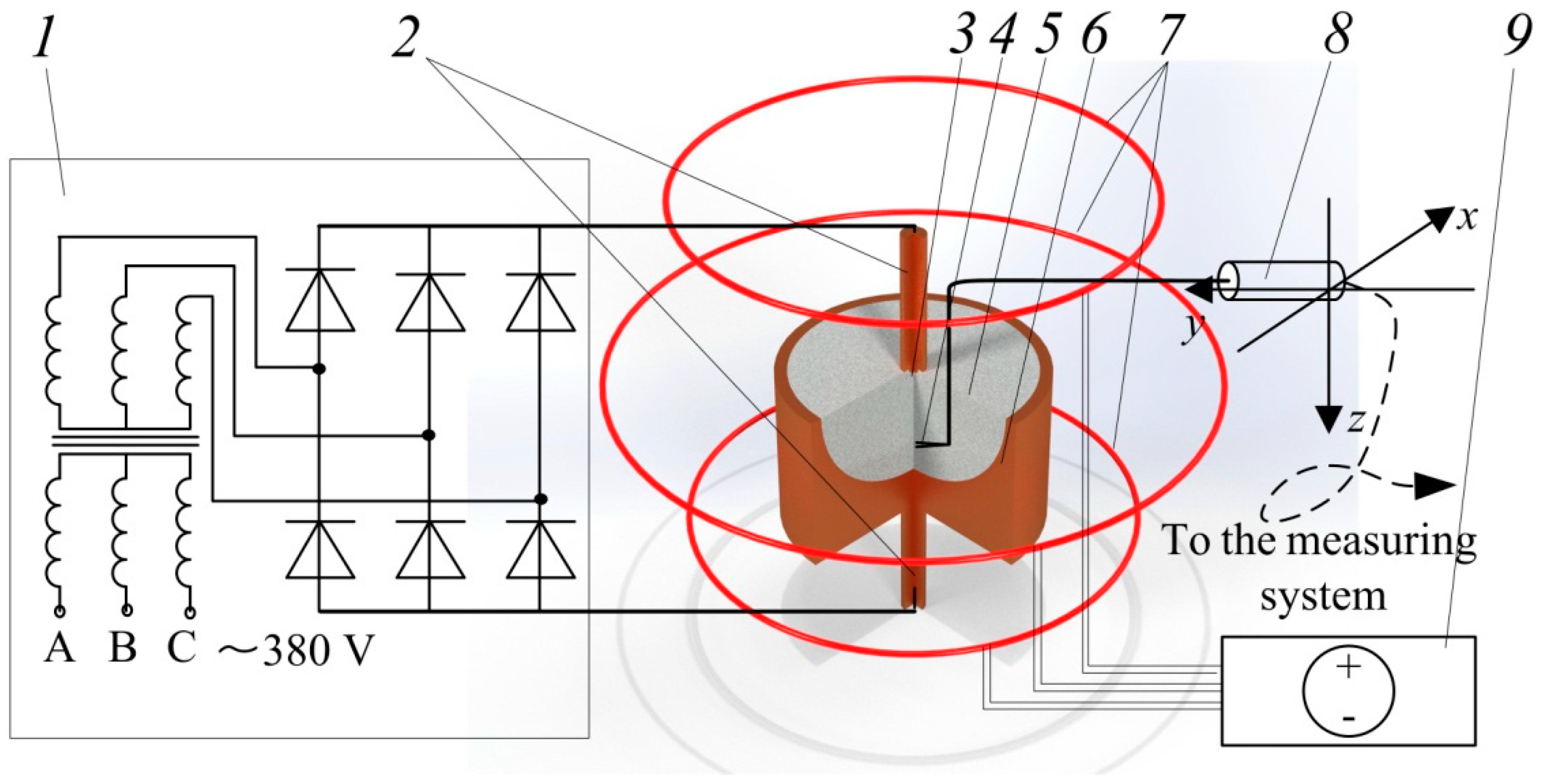
3. Experimental Setup

The experiments were carried out on the experimental setup shown in Figure 2. An eutectic alloy In-Ga-Sn with content by weight Ga—67%, In—20.55, Sn—12.5% (melting temperature + 10.5 °C) was used as a working liquid [16]. The alloy was filled into a hollow copper hemispherical container with a diameter of 188 mm, which served as a large electrode. The small electrode was also made of copper, in the form of a convex hemisphere 5 mm in diameter. The electrode was immersed in the liquid to a depth of radius. The accuracy of determining the immersion depth was controlled using a micrometer.

A current source based on a three-phase six-half-period rectifier assembled according to Larionov’s scheme was used to power the setup. The rectifier input current was controlled by three connected single-phase autotransformers. The Larionov rectifier circuit provides a constant current with ripples of ~13%, the source allows you to obtain a constant current of up to 1500 A, in our experiments the current varied in the range of 100–450 A for reasons that will be described below.

To compensate for the axial component of the Earth’s magnetic field, a system of Maxwell coils was assembled. Maxwell coils are three rings, two with radii a—174 mm, and a turn between them with a radius $a\sqrt{(}4/7)$= 230 mm, and located at a distance $a\sqrt{(}3/7)$ along the axis (~150 mm). In our case, each ring consisted of four turns of a copper wire with. A current I = 3.70 A is supplied to a pair of side coils, and a current 2.83 A (49/64I) to the middle one. Such a system makes it possible to obtain a sufficiently uniform magnetic field both along the z axis and along the radius r, in contrast to Helmholtz coils. (Helmholtz coils are a system of two rings with a current of radius R located at a distance R along the axis from each other and allowing a constant magnetic field to be obtained only along the z axis). The coils were powered from two stabilized current sources.

The resulting axial magnetic field did not exceed 3 μT and was monitored using a LakeShore DSP475 magnetometer. In order to check the uniformity of the field, the calculation of the field created by the Maxwell and Helmholtz coils was carried out. The axial and radial components of the magnetic field of a circular loop with current (in cylindrical coordinates) can be found by the formulas [17]

$$B_r=\frac{{\mu }_{0}I}{4\pi }\frac{2z}{r\sqrt{{\left(a+r\right)}^2+z^2}}\left(-K+\frac{a^2+r^2+z^2}{{\left(a-r\right)}^2+z^2}E\right),$$

(10)

$$B_z=\frac{{\mu }_{0}I}{4\pi }\frac{2}{r\sqrt{{\left(a+r\right)}^2+z^2}}\left(K+\frac{a^2-r^2-z^2}{{\left(a-r\right)}^2+z^2}E\right).$$

(11)

Here a is the radius of the ring, I is the current in the ring, and K and E are complete elliptic integrals of the first and second kind.

According to the principle of superposition, the magnetic field is equal to the sum of the magnetic fields, then the total field of three coils is equal to B = B_coil1 + B_coil2 + B_coil3 with corresponding currents and radii, where B_coil1,2,3 is the magnetic field of the coil.

The Figure 3 shows the calculated distribution of the magnetic field (z-component) in the area of the container with liquid metal created by the Maxwell coils. The field generated by the Helmholtz coils is also shown for comparison. Blank space—data out of the range. The inhomogeneity of the Maxwell coil is approximately 0.4%, and the Helmholtz coil is 1.6%.

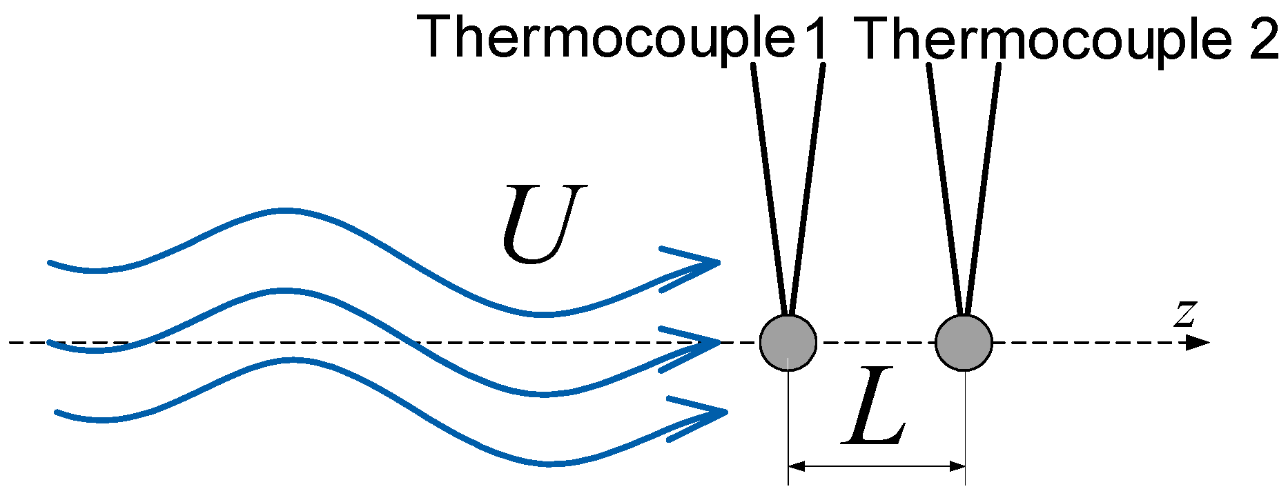
4. Measurement Technique

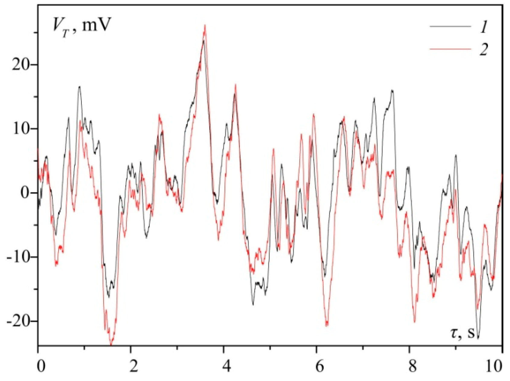
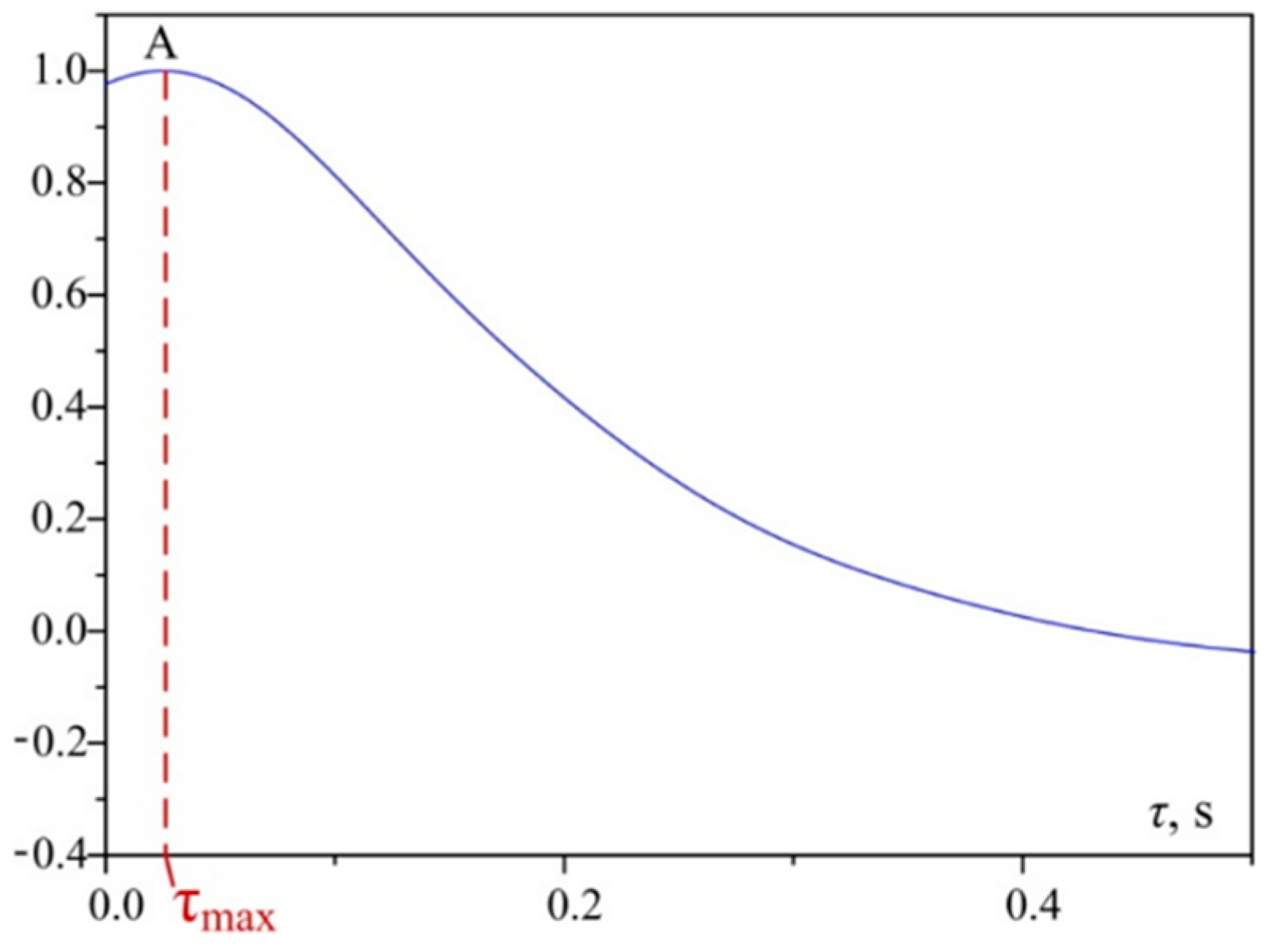
4.1. The Principle of the Thermocorrelation Method

A thermocorrelation probe was used to measure the velocity; the probe diagram is shown in the figure. The probe consists of two thermocouples located on the flow axis at a distance L from each other and operates as follows. Turbulent fluid flow moves in the direction of the z-axis. Turbulent pulsation comes first to thermocouple 1, then after a while to thermocouple 2. See Figure 4. The signals from the thermocouples are fed to the analog-to-digital converter and are recorded for a certain period of time (30–120 s). Next, the cross-correlation function (CCF) is calculated using two signals. The maximum of the CCF corresponds to the average time ${\tau }_{\max }$ taken by the pulsation to reach the second thermocouple, so the velocity in z-direction can be defined as $U_z=L/{\tau }_{\max }$.

Example of the temperature oscillograms is shown in Figure 5. Since the absolute temperature values are not important for determining the speed, the voltage was not converted into temperature, and the temperature signal is shown in the graph in millivolts. An example of the cross-correlation function is shown in Figure 6.

The probe was installed so that the thermocouples were positioned vertically on the flow axis. The probe uses copper–constantan thermocouples with wire diameters of 0.07 and 0.08 mm, and the junction size does not exceed 0.2 mm. The distance between the thermocouples was 4.7 mm (measured under the microscope). A photograph of the probe is shown in Figure 7.

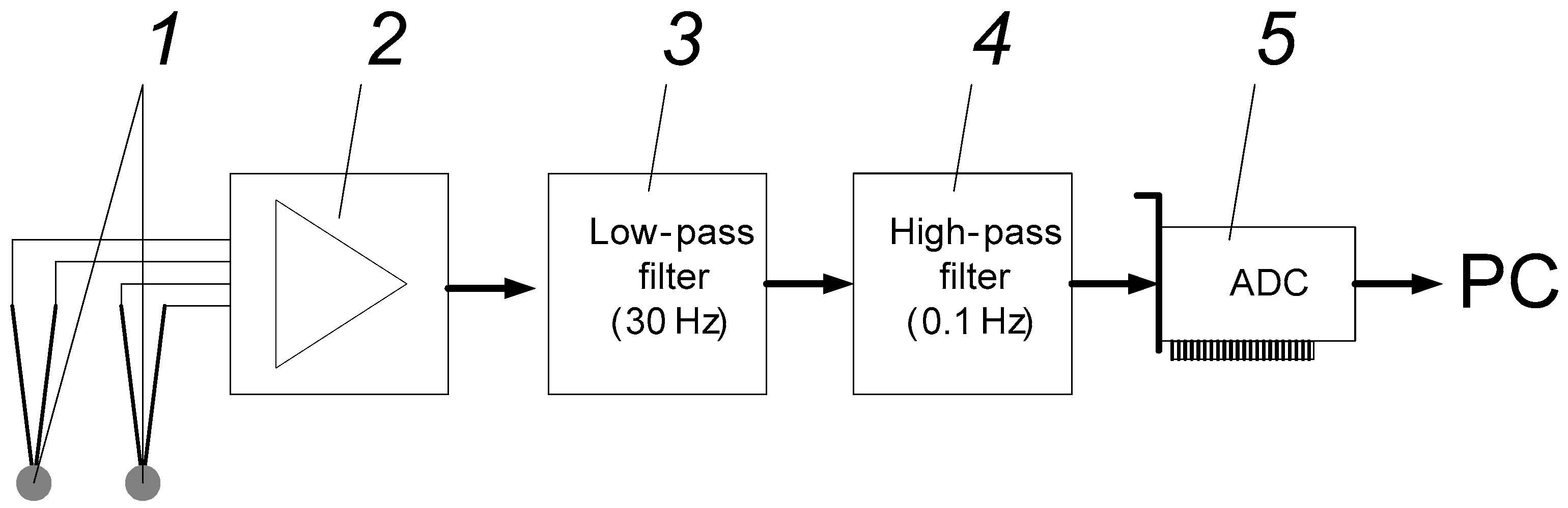
4.2. Measuring Circuit

Let’s consider in detail the measuring circuit. The measuring circuit is shown in Figure 8. In order to reduce the influence of interference from the electrical network, the power supply of the amplifier and filters was carried out from batteries, and the personal computer was connected through an isolation transformer.

In order to find out the optimal implementation time, experiments were carried out to determine the scatter of readings from the duration of implementation. It was clear from the experiment that the implementation duration of 120 s is sufficient for the correct averaging of the velocity values. In further experiments, we used this value for the implementation time.

4.3. Measurement Procedure

Obtaining the dependence of the axial velocity on the current in modes with and without magnetic field compensation. The measurements were carried out as follows. The probe was immersed 20 mm deep (at a depth of 20 mm there was a central point between the thermocouples) on the container axis. Then the current was switched on and five measurements were carried out, each measurement lasting 120 s. At the end of the measurement, the current rose to the next required level and was turned off, a pause was maintained for five minutes, then the current was turned on, and the measurement was performed again.

Two series of experiments were carried out, in the first the Maxwell coils were turned on, in the second they were turned off. The results are shown in Figure 9.

Further, two series of measurements of the dependence of the axial velocity on the depth were carried out. The measurements were also carried out in modes with and without compensation of the Earth’s field. The results are shown in Figure 10.

The measurement error includes two components—instrumental and random. The instrumental error is determined by the accuracy of setting the distance between the thermocouples and the accuracy of determining the time (corresponding to the maximum of the correlation function) using the ADC. These values are significantly less than the random error caused by flow instability. For each set of five measurements, the absolute error was calculated as

$$\Delta {\tau }_{\max }=\frac{T_{\mathrm{St}}{\sigma }_N}{\sqrt{N}},$$

where T_St—Student’s coefficient, ${\sigma }_N$—standard deviation, and N—number of measurements. Error bars for velocity are presented on the graphs. We can see flow is rather unstable and contains large-scale fluctuations in some modes. For most measurements, the error does not exceed 5–15%, but in the areas of maximum speed values it can reach 35%.

Figure 11 and Figure 12 show typical spectra of temperature pulsations at different currents. It is noticeable that an increase in the current leads to a broadening of the spectrum. Maxwell coil on mode results in spectrum narrowing.

5. Discussion

Let’s analyze these results. In the mode with compensation of the Earth’s MF, we observe an increase in the velocity with an increase in the current, which is quite obvious, but the nature of this growth turns out to be somewhat unexpected. In [18], it is shown that in the Stokes regime (linear, when the influence of the nonlinear terms of the Navier–Stokes equation is negligible), the dependence of the velocity on the electric current has the form, U ~ I², and the developed electric vortex flow has the form of the dependence U ~ I. It can be expected that turbulence takes away energy from the averaged flow and this dependence will be weaker than linear, but, on the contrary, this dependence can be approximated by a power function with exponent ~3/2. It can be assumed that the Stokes regime continues up to the currents under consideration, but an elementary analysis shows that in such a system the Stokes regime takes place up to the number S = 1000, i.e., up to current ~ 1 A.

In the mode without compensation of the Earth’s MF, we observe a decrease in speed compared to the mode with compensation, this is explained by the fact that the azimuthal force driving the fluid into rotation creates a secondary near-bottom vortex (akin to Taylor’s vortices) directed opposite to the main electric vortex flow. The interaction of two vortices can lead to self-oscillations (as shown in [19]) and, in the case of a small external magnetic field, to a weakening of the axial velocity.

We also measured the axial speed along the axis at currents of 100 A, 250 A, and 450 A.

The results are shown in the figure. In compensated mode, there is a decrease in speed along the entire axis.

Upon reaching a current of 500 A, the liquid separates from the electrode due to the pinch effect and a spark appears (Figure 13). The mechanism of this phenomenon is as follows. The electromagnetic force is directed downward and towards the center, and grows quadratically depending on the electric current. The force squeezes the liquid away from the electrode, reducing the contact area, a decrease in the contact leads to an increase in the current density and a further increase in the force. At some point, the electromagnetic force can no longer be balanced by gravity and the process becomes unstable. The critical current depends on the size of the small electrode and increases with its diameter. This problem is discussed in [20]. The photograph shown in the figure shows an electrical breakdown at a current of 500 A.

6. Conclusions

• In this work, the thermocorrelation method was first applied to study the velocity in a current-carrying medium. The method has shown its efficiency in difficult measurement conditions and can be recommended for use in industry. Nevertheless, the excessive duration of one measurement limits the application of the method in non-stationary processes. We have found that 120 s is sufficient to average the speed values correctly.
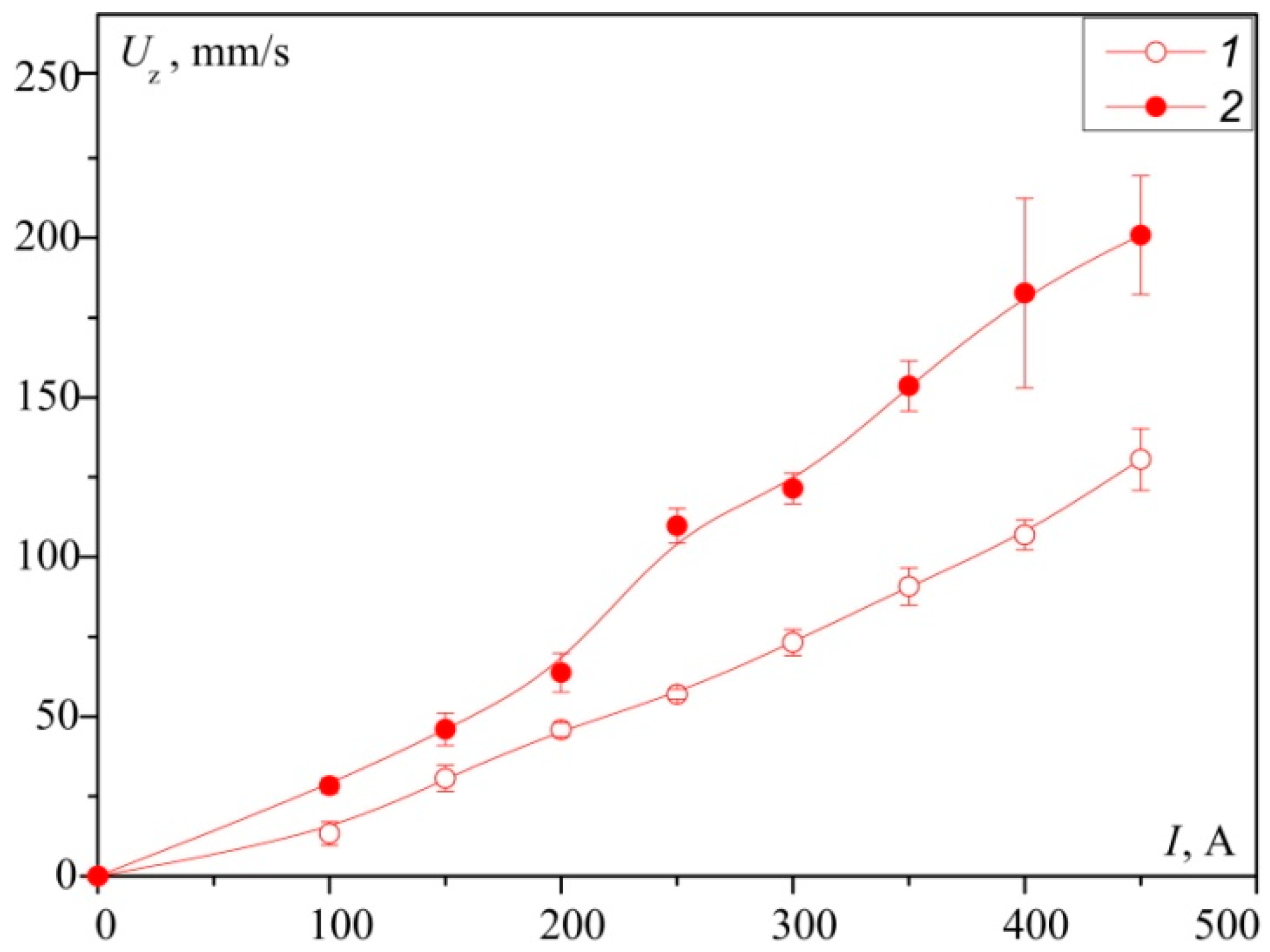
• The measurement of the dependence of the velocity of the electric vortex flow in the hemisphere depending on the current was carried out; it was found that up to the maximum possible currents in this geometry (450–500 A, higher current creates the electric arc), the dependence has a power-law character, with an exponent close to 3/2.
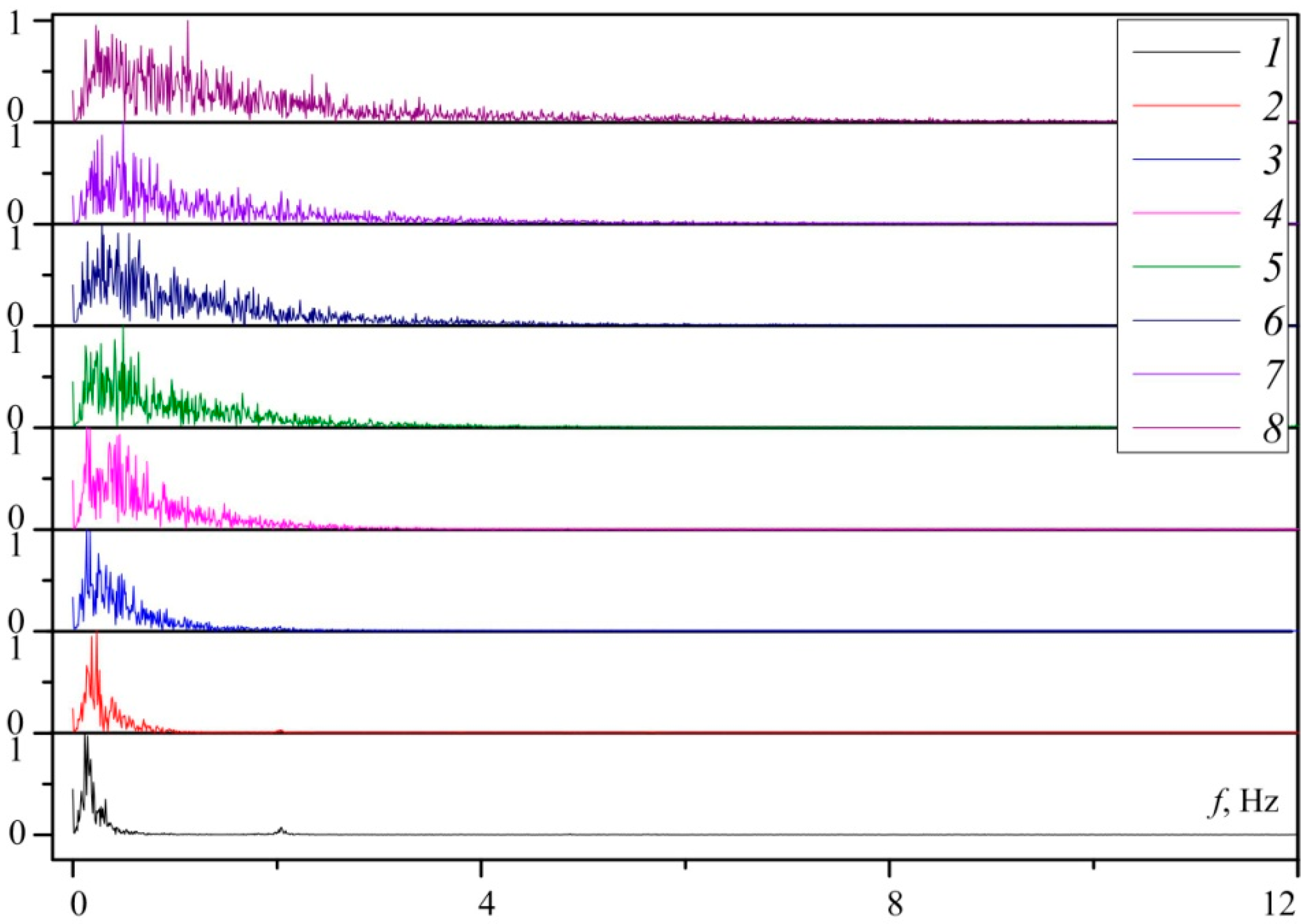
• It was found that turbulent pulsations in such a system are limited from above by a frequency of 5 Hz.
• Even at relatively high currents (up to 450 A), the influence of the Earth’s magnetic field is significant and leads to a noticeable decrease in the axial flow velocity. Thus, any measurements in an axisymmetric electric vortex flow in a similar geometry made without compensation of the Earth’s magnetic field cannot be considered reliable.

Industrial Application Notes

For industrial metallurgical applications, this method is probably the only adequate one; when using high-temperature thermocouples (tungsten–rhenium), the method can be used to determine the velocity in melts up to temperatures of 1800 °C, besides, thermocouples are quite cheap, and the sensor design is very simple. The increase in the number of thermocouples in the probe to four, allows, if necessary, to simultaneously measure three velocity components.

Geometry similar to that described in the article is typical for electric welding tasks. Since the electric vortex flow in such a geometry (due to the presence of a converging flow) is extremely sensitive to the external magnetic field causing the rotation of the melt, then even a weak magnetic field of the Earth should be taken into account in the calculations of such problems.

References

1. Bojarevish, V.; Freibergs, Y.; Shilova, E.I.; Shcherbinin, E.V. Electrically Induced Vortical Flows; Kluwer Academic Publishers: Dordrecht, The Netherland; Boston, MA, USA; London, UK, 1989. [Google Scholar]
2. Platnieks, I.; Uhlmann, G.J. Hot-wire sensor for liquid sodium. Phys. E Sci. Instrum. 1984, 17, 862–863. [Google Scholar] [CrossRef]
3. Thess, A.; Votyakov, E.V.; Kolesnikov, Y. Lorentz Force Velocimetry. Phys. Rev. Lett. 2006, 96, 164501. [Google Scholar] [CrossRef] [PubMed] [Green Version]
4. Cramer, A.; Eckert, S.; Gerbeth, G. Flow measurements in liquid metals by means of the ultrasonic Doppler method and local potential probes. Eur. Phys. J. Spec. Top. 2013, 220, 25–41. [Google Scholar] [CrossRef]
5. Zhilin, V.G.; Ivochkin, Y.P.; Oksman, A.A.; Lurin’sh, G.R.; Chaikovskii, A.I.; Chudnovskii, A.Y.; Shcherbinin, E.V. An experimental investigation of the velocity field in an axisymmetric electrovortical flow in a cylindrical container. Magnetohydrodynamics 1986, 22, 323–328. [Google Scholar]
6. Termaat, K.P. Fluid flow measurements inside the reactor vessel of the 50 MWe Dodewaard nuclear power plant by cross-correlation of thermocouple signals. J. Phys. E Sci. Instrum. 1970, 3, 589–593. [Google Scholar] [CrossRef]
7. Belyaev, I.A.; Razuvanov, N.G.; Sviridov, V.G.; Zagorsky, V.S. Temperature correlation velocimetry technique in liquid metals. Flow Meas. Instrum. 2017, 55, 37–43. [Google Scholar] [CrossRef]
8. Malyshev, K.; Mihailov, E.; Teplyakov, I. Analytical study of the velocity and pressure of the electrovortex flow in hemispherical bowl in a Stokes approximation. J. Phys. Conf. Ser. 2020, 1683, 02207. [Google Scholar] [CrossRef]
9. Shatrov, V.; Gerbeth, G. Stability of the electrically induced flow between two hemispherical electrodes. Magnetohydrodynamics 2012, 48, 469–483. [Google Scholar] [CrossRef]
10. Chudnovsky, A.; Ivochkin, Y.; Jakoviċs, A.; Pavlovs, S.; Teplyakov, I.; Vinogradov, D. Investigations of electrovortex flows with multi electrode power supply. Magnetohydrodynamics 2020, 56, 487–498. [Google Scholar]
11. Shcherbinin, E. Induction-free approximation in the theory of electrovortex flows. Magnetohydrodynamics 1991, 27, 308–311. [Google Scholar]
12. Teplyakov, I.; Vinogradov, D.; Ivochkin, Y.; Kharicha, A.; Serbin, P. Applicability of different MHD approximations in electrovortex flow simulation. Magnetohydrodynamics 2018, 54, 403–416. [Google Scholar]
13. Zhilin, V.; Ivochkin, Y.; Teplyakov, I. The problem of swirling of axisymmetric electrovortex flows. High Temp. 2011, 49, 927–929. [Google Scholar] [CrossRef]
14. Kharicha, A.; Wu, M.; Ludwig, A.; Karimi-Sibaki, E. Influence of the earth magnetic field on electrically induced flows. J. Iron Steel Res. Int. 2012, 19, 63–66. [Google Scholar]
15. Vinogradov, D.; Ivochkin, Y.; Teplyakov, I. Influence of the Earth’s Magnetic Field on the Structure of the Electrovortex Flow. Dokl. Phys. 2018, 483, 24–27. [Google Scholar] [CrossRef]
16. Prokhorenko, V.; Ratushnyak, E.; Stadnyk, B.; Lakh, V.; Koval, A. Physical properties of thermometric alloy In-Ga-Sn. High Temp. 1970, 8, 374–378. [Google Scholar]
17. Landau, L.D.; Lifshitz, E.M. Electrodynamics of Continuous Media, 2nd ed.; Nauka: Moscow, Russia, 1992; p. 164. [Google Scholar]
18. Chudnovskii, A.Y. Evaluating the intensity of a single class of electrovortex flows. Magnetohydrodynamics 1989, 25, 406–408. [Google Scholar]
19. Ivochkin, Y.; Teplyakov, I.; Vinogradov, D. Investigation of selfoscillations in electrovortex flow of liquid metal. Magnetohydrodynamics 2016, 52, 277–286. [Google Scholar] [CrossRef]
20. Kharicha, A.; Teplyakov, I.; Ivochkin, Y.; Wu, M.; Ludwig, A.; Guseva, A. Experimental and numerical analysis of free surface deformation in an electrically driven flow. Exp. Therm. Fluid Sci. 2015, 62, 192–201. [Google Scholar] [CrossRef]
Figure 1. Scheme of the electrovortex flow.
Metals 11 01806 g001
Figure 2. Experimental setup. 1—power supply (thre-pase rectifier); 2—current leads; 3—small electrode; 4—thermocouple probe; 5—eutectic alloy In-Ga-Sn; 6—big electrode-container; 7—Maxwell coil; 8—3D coordinate system for probe; and 9—power supplu for Maxwell coil.
Metals 11 01806 g002
Figure 3. Distribution of the magnetic field of (a) Maxwell coil; and (b) Helmholtz coil.
Metals 11 01806 g003
Figure 4. Scheme of the thermocorrelation method for measuring the velocity.
Metals 11 01806 g004
Figure 5. Temperature signal from two thermocouples (after amplification, filtering, and DC trimming) at the current 450 A.
Metals 11 01806 g005
Figure 6. Cross-correlation function of the two temperature signals.
Metals 11 01806 g006
Figure 7. Photo of the thermocorrelation probe over the surface of the liquid metal. 1—thermocouples; 2—small electrode with a drop of liquid metal; 3—probe holder; and 4—In-Ga-Sn.
Metals 11 01806 g007
Figure 8. Measuring circuit. 1—thermocouples; 2—amplifier; 3—filter; 4—filter; and 5—analog-to-digital converter inserted into a personal computer.
Metals 11 01806 g008
Figure 9. The dependence of the axial velocity on the electric current at depth z = 20 mm.
Metals 11 01806 g009
Figure 10. The dependence of the axial velocity on the depth z at a different currents. Index a—Maxwell coil is turned on, b—off. 1—100 A; 2—250 A; and 3—450 A.
Metals 11 01806 g010
Figure 11. Spectra of temperature pulsations at different currents. Maxwell coil is turned off. 1—100 A; 2—150 A; 3—200 A; 4—250 A; 5—300 A; 6—350 A; 7—400 A; and 8—450 A.
Metals 11 01806 g011
Figure 12. Spectra of temperature pulsations at different currents. Maxwell coil is turned on. 1—100 A; 2—150 A; 3—200 A; 4—250 A; 5—300 A; 6—350 A; 7—400 A; and 8—450 A.
Metals 11 01806 g012
Figure 13. Appearing of the sparkle above a liquid surface at the current 500 A.
Metals 11 01806 g013
Publisher’s Note: MDPI stays neutral with regard to jurisdictional claims in published maps and institutional affiliations.