1. Introduction
In today’s modern and innovative times, more and more demands are placed on industrially used materials. In addition to that, materials are often required to fulfil conflicting properties, such as, e.g., to have high yield strength, ultimate tensile strength, and simultaneously also good ductility, formability, or weldability. At the same time, high attention is paid as well to the price of these materials, which increases with the amount of used alloying elements. Therefore, newly developed materials use a grain-boundary strengthening and belong to the group of so-called HSLA (High Strength Low Alloy) steels. These are usually microalloyed fine-grained steels that are alloyed by very low contents of elements such as, e.g., V, Ti, and Nb. Such elements form fine carbides, nitrides, or carbonitrides and contribute to the grain refinement and strengthening of the matrix [
1,
2]. It also has a secondary effect in increased values of the yield strength and ultimate tensile strength, but there is also lower values of transient temperature and brittle fracture properties [
3,
4]. Moreover, despite all of the advantages mentioned above, these steels also keep their price low, because they are derived from the prices of conventional carbon steels due to the low amount of alloying elements.
Although many people think of HSLA steels primarily as high-strength steels, typically with yield strengths highly exceeding 550 MPa, micro-alloyed steels are very popular and often used in the production of structures having yield strength below 550 MPa. Among these can be found, for example, thermomechanically processed steels of the S355MC, S420MC, and S460MC types. As a reason why these steels gradually substitute the common structural steels (e.g., type S355J2), there is their better cold formability and constant technological processability given by stronger demands to meet their chemical composition.
Generally, HSLA steels reveal good weldability, but the amount of heat input into the weld should be limited and should not exceed 15 kJ·cm
−1. In the case of high-strength steels, it is recommended to further reduce such heat input value. As a reason for that, there is the intensive grain coarsening in the heat-affected zone (HAZ) at temperatures over 1100 °C. These are temperatures at which occurs dissolving of the fine precipitates that stabilize grain boundaries and structure. Such an issue is quite a closely monitored topic that confirms also a great number of published articles dealing with the grain coarsening intensity [
2,
4,
5], changes in strength and brittle-fracture properties [
4,
6,
7], or structural changes that occur in the heat-affected zone—HAZ [
8,
9]. However, not many papers are devoted to the influence of welding on changes in the fatigue life of welded joints for HSLA steels with a yield strength lower than 550 MPa [
10], despite the fact that these materials and welded structures are used very often—for example, in land transportation [
11] (i.e., in areas of quite intense dynamic loading). Nevertheless, more works are devoted to welded joints of high-strength materials [
12,
13,
14] and again despite the fact that the notch effect arising from the weld geometry reduces its fatigue life to the level of welded joints with lower values of yield strength.
Most works dealing with the fatigue tests of HSLA steel welded joints [
12,
15] use for fatigue tests either butt welds or flat specimens to which a temperature cycle is applied. This is a little bit strange, because most dynamically loaded structural units used in the field of land transportation contain mainly fillet welds, despite their lower static and dynamic load capacity. Other works then deal, e.g., with the influence of load cycle asymmetry—stress ratio R [
16] or fatigue life prediction using the energy approach [
13].
The aim of the research described in the following sections, was to point out that there have not been almost any papers published dealing with the welded joints from steel S460MC. Thus, the aim was to assess the heat input influence on the fatigue life of fillet welded joints that are structurally designed to match the joints commonly used in industrial production. As a result, complete S-N curves were obtained at stress amplitudes corresponding to the range of loading cycles from 10
4 up to 10
7. Most authors studying the HSLA steel welds’ fatigue life usually focus on the butt welds from the high-strength steels. If they deal with the fillet welds, there are performed fatigue tests at selected stress amplitudes within the loading cycles from 10
5 up to 2 × 10
6 [
17], and for the remaining stress amplitudes are just used an approximation of the fatigue curves or there are used cruciform welds at testing [
18,
19]. These welds are due to their symmetry of four fillet welds more suitable in light of our own testing. However, they are completely unsuitable from the welding point of view, especially for the fine-grained steels. In addition to that, very important is also knowledge about mutual proportion among the yield strength, fatigue limit of the base material σ
c(BM), and fatigue limit of the fillet welded joint σ
c(W) from steel S460MC and its comparison with the (ultra) high-strength steels, presented by other authors.
5. Fatigue Life Determination for Tested Fillet Welds
As in the case of the base material, a servo-hydraulic testing machine INOVA FU-O-1600-V2 (INOVA GmbH, Bad Schwalbach, Germany) in the controlled force mode was used to determine the fatigue life of welded joints. Based upon the results of the initial fatigue tests (for base material), the samples were loaded under the following stress amplitudes: 300, 240, 170, 152.5, 135, 117.5, 100, 82.5, 74 and 65 MPa. Furthermore, in this case, all samples were subjected to a fully reversed harmonic cycle (purely alternating stress) with stress ratio R = −1. Compared to the fatigue testing of the base material, the loading frequency was lower by 20 Hz due to the larger cross-section area of testing samples—thus also higher force amplitudes. This causes an increase of the strain rate in the sample, which led to a heating of the sample surface under a frequency of 40 Hz. As in the case of the base material, there were firstly carried out primary tests of samples with double-sided fillet welds and having corresponding dimensions and a preparation method that was subsequently used for our own experiment. The grinded surface of the sample was again scanned by an infrared pyrometer on the interface between the weld bead and base material. Such primary testing was performed at stress amplitudes 300 and 175 MPa. The same test termination criteria were also used in this kind of fatigue test—fatigue crack initialization or achieving the fatigue limit at 107 cycles, where testing material does not show a distinct fatigue limit σC.
Identification of the crack initiation was realized on the basis of setting the testing machine INOVA FU-O-1600V2 control program. The criterion of the so-called unstable increase of deformation during the test was chosen to terminate our own testing procedure. This criterion is based on the continuous monitoring of the sample deformation (to be specific, its deviation) necessary to achieve the required loading force. Such monitored strain magnitude is averaged from the last 500 test cycles and thus allows the elimination of the strengthening or recovery effect of the sample without termination of the test. The testing procedure was terminated when deformation revealed an abnormal increase of more than 20% compared to the average of the last 500 cycles. After termination of every test, there was loaded a course force vs. displacement by return, from which it was possible to identify the moment of crack initialization. In all cases presented in this paper, crack in the joint was identified after test termination.
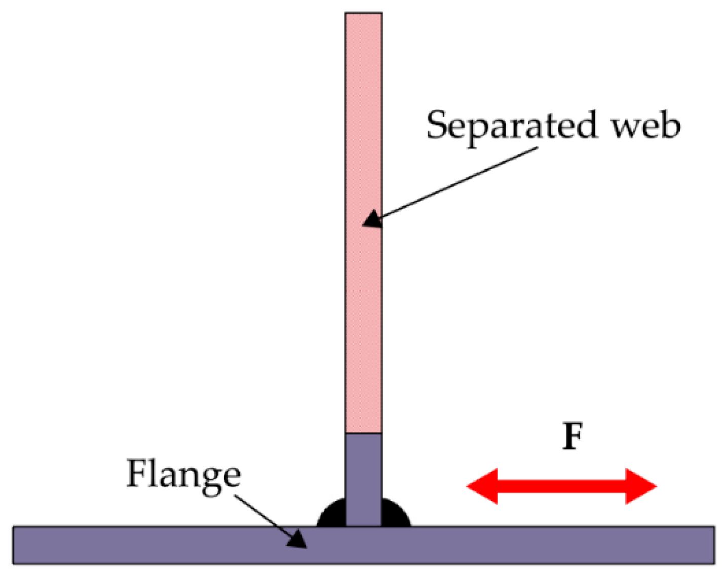
All welds were loaded in the flange direction, as it is schematically shown in
Figure 12. Subsequently,
Table 7 then gives an overview about fatigue test results for all tested welds.
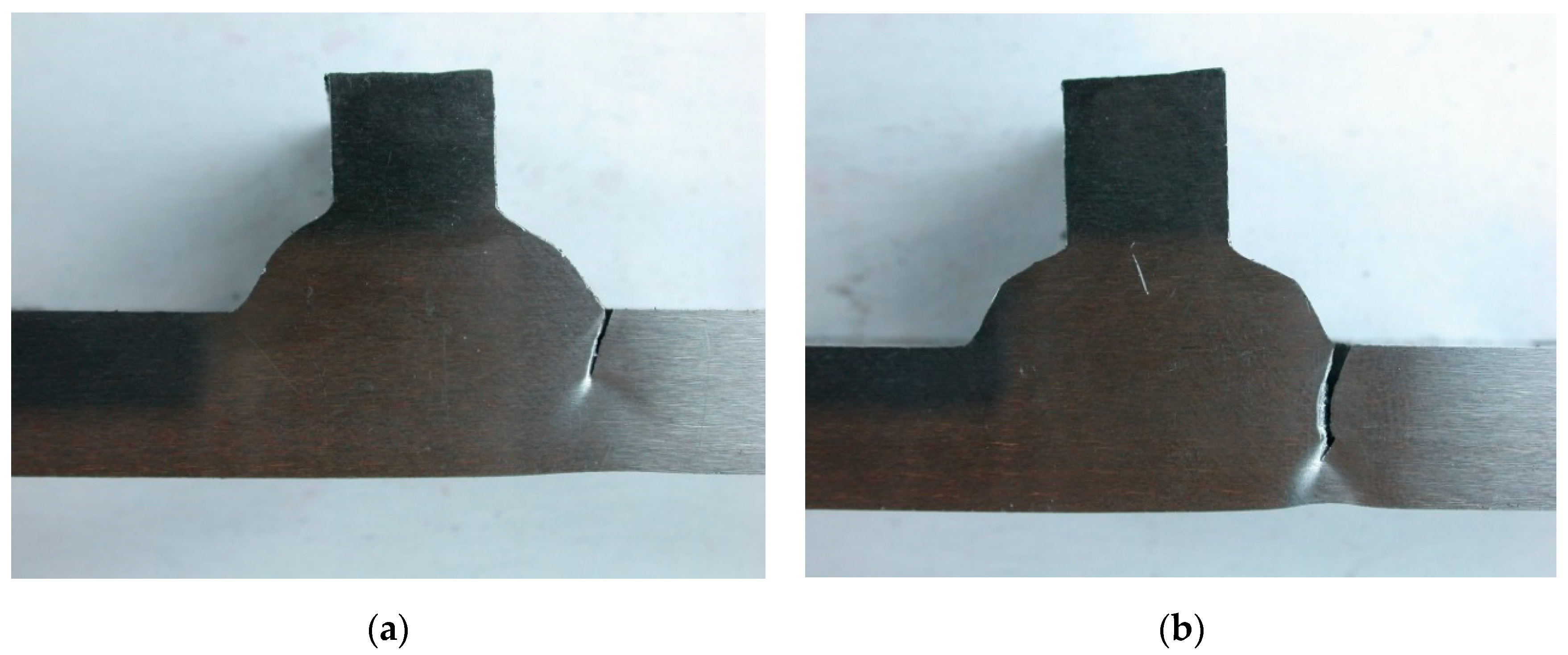
In all cases, the location of the fatigue failure of the testing sample was determined, and the crack was initiated at the interface between the flange and the weld bead, as it is obvious from
Figure 13a for Weld Q12 (stress amplitude σ
A = 300 MPa) and in
Figure 13b for Weld Q12 (stress amplitude σ
A = 74 MPa). In all fatigue failures, the crack grew perpendicularly to the loading force direction. In addition to that, a fatigue limit σ
C = 65 MPa was determined for all fillet welds, which represents only 20% of the fatigue (endurance) limit σ
C measured for the unaffected base material.
Results summarized in
Table 7 were subsequently plotted in the S-N curves (log-log scale) to determine fatigue characteristics via their approximation according to the so-called Basquin’s equation (Equation (1)):
In Equation (1), σf (MPa) is the fatigue strength coefficient and b (1) is the fatigue strength exponent. By these approximation quantities can be characterized the whole course of the fatigue life (via stress amplitude σA as the independent variable) vs. cycles to failure Nf (independent variable). However, in this case are instead of cycles to failure Nf are used so-called reversals to failure—thus 2Nf.
Generally, Basquin’s equation mathematically means the power-law function. Because of better clearness (specially to cover large values of reversals to failure), in graphs this equation is shown in log-log scales, thus as the linear function. In
Table 8 are summarized results of fatigue strength coefficient σ
f and fatigue strength exponent b for monitored heat input values.
6. Discussion
The welding heat input strongly affects the basic mechanical properties (e.g., such as yield strength, ultimate tensile strength, and ductility) of fine-grained steels [
4,
6,
20,
21]. Higher heat input values cause a longer exposition to high temperatures, which means more intense changes that can occur in HAZ of welds. In addition to that, these changes influence not only the mechanical properties, but also have a very significant effect on the notch toughness value [
4,
6,
22].
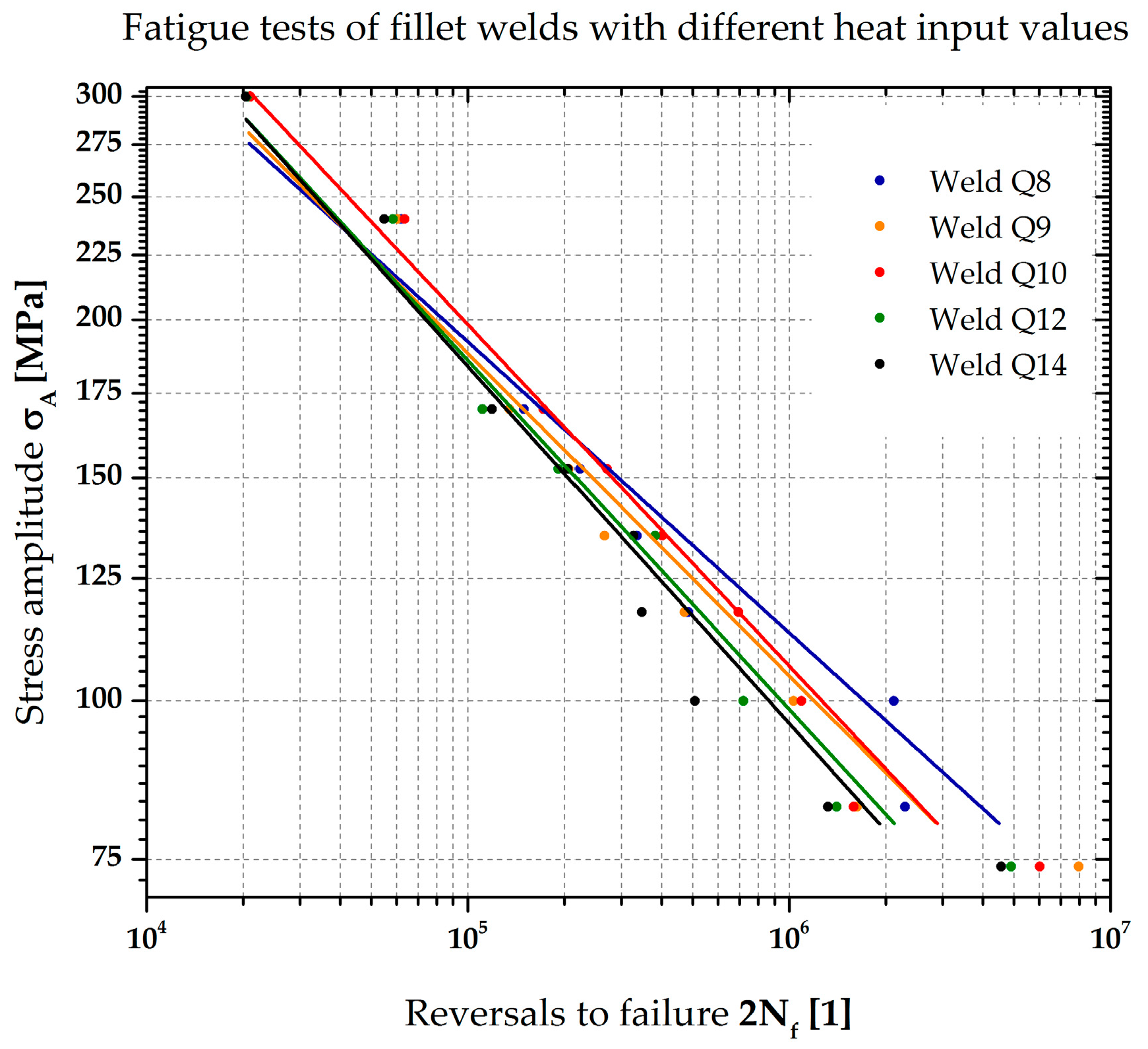
In addition to the changes that occur in the HAZ, other aspects also have an effect on the reduction of fatigue life in the case of cyclic loading. Especially important is the effect of the weld bead geometry, because it defines the notch effect at cyclic loading as well as, e.g., the magnitude of angular deformations after welding, causing occurrence of the combined stress (tension, compression, and bending). To define the influence of the individual aspects mentioned above is very difficult under dynamic loading, especially in the case of fillet welds. To keep the boundary conditions as accurate as possible, all samples used for fatigue tests had exactly the same dimensions, grinded edges with the same surface roughness, and completely identical loading conditions (clamping force, frequency, sample centering in jaws, and so on). Regarding the actual knowledge in the field of welding fine-grained thermomechanically processed structural steels, there would be expected a reduction of the welded joint fatigue life with increasing heat input value. This assumption is also confirmed in this research by the slope of linear fitting, as shown in
Figure 14, expressed via values σ
f and b computed from Basquin’s equation (linear fitting of measured data from
Table 7). The lowest slope (b = −0.230) was computed for tested welded joints with the heat input of Q = 8 kJ·cm
−1. Generally stated, the higher the heat input value, the higher the slope of the obtained trends. These results are usually used by designers when designing the maximal allowable loads of different steel welded structures.
However, from
Figure 14 is also evident that different slopes of fitted linear trends no longer fully confirm the assumption about reduction in the fatigue life with increasing heat input value in the whole range of applied stress amplitudes. In the area of limited life, and especially in its initial phase at higher stress amplitudes σ
A (up to 225 MPa), better results were achieved with higher heat input values—thus for Q10, Q12, and Q14. This would correspond to weldments with an expected number of cycles not exceeding 45,000 cycles. On the other hand, from this value slopes of applied linear trends behave according to the theoretical assumptions. A partial exception can be observed only in the case of the trend determined for Weld Q10, where are achieved the lower values of fatigue life—lower than 162 MPa compared to Weld Q8 and lower even than 83 MPa compared to Weld Q9. This partial anomaly is probably caused by the given weld geometry, as shown in
Table 6, where the highest value of radius R was measured for Weld Q10 at the interface between the weld and flange. Thus, there is partially reduced the notch effect as a stress concentrator under cyclic loading.
However, taking into account the error measurement of the fatigue strength coefficient and especially the fatigue strength exponent, as shown in
Table 8, which vary from 6% to 9% for the individual heat input values, it can be stated that heat input value does not influence the change of fatigue limit in the low cycle fatigue area. On the other hand, influence of the heat input can be observed in the high cycle fatigue area, where the difference of fatigue limit σ
c(W) for curves with the heat input value Q = 8 kJ·cm
−1 and Q = 14 kJ·cm
−1 is about 30%, even when the maximal overlap confidence intervals are taken into account. Based on the above findings, it could be expected that heat input value will also affect the magnitude of the fatigue limit σ
c(W). Nevertheless, as it is shown in
Table 7, this magnitude of σ
c(W) for cycles to failure N
f > 10
7 was the same (65 MPa) for all tested heat input values. Based upon the cycles to failure measured at stress amplitude σ
A = 74 MPa, it can be assumed that for welded joints having lower heat input values, the fatigue limit would be reached even at stress amplitudes higher than 65 MPa.
Comparing the obtained results with other similar works, it can be stated that different research works in the field of HSLA steels’ fatigue life are carried out by many researchers, but not for fillet welds. Šebestová et al. [
10], determining the fatigue life of welds for S460MC and S700MC steels, performed by the Laser-hybrid method, measured for base material steel 460MC a fatigue limit of σ
c = 310 MPa and fatigue limits of butt welds (in dependence on the heat input value) of about 100 MPa. The fatigue limit of base material was lower by 30 MPa than fatigue limit σ
c measured here. The reason for that was most likely the square cross-section area of the testing samples, where fatigue cracks can more easily initiate in the corners of the sample. The fatigue (endurance) limit of butt welds is usually 2 to 3 times higher than that of fillet welds. Lahtinen et al. [
12] tested fatigue properties of butt welds made of S700MC steel and welded by the MAG method. The effect of the input heat was there expressed by a different time value t
8/5. As in our case, it was confirmed that the effect of the heat input value (expressed by the slope of fitting linear trends arising from the measured values) has a much higher influence just at lower stress amplitudes corresponding to the cycles to failure of about 180,000 cycles.
Another important finding is also the mutual ratio between the yield strength of tested material
Re, fatigue limit of the base material σ
c(BM), and fatigue limit of the welded joint σ
c(W). These ratios are for the tested material S460MC as follows: σ
c(BM)/
Re = 0.625; σ
c(W)/
Re = 0.119; and σ
c(W)/σ
c(BM) = 0.193. For steel S700MC they are: σ
c(BM)/
Re = 0.583 [
14]; σ
c(W)/
Re = 0.102 [
17]; and σ
c(W)/σ
c(BM) = 0.171. From these ratios it is evident that applications of materials with higher yield strength does not automatically mean achieving relatively higher values of welded joint fatigue life. Therefore, it is very important to consider other aspects, such as the structural design of joints, welding parameters influencing weld geometry (notch effect), as well as our own welding method causing angular deformation.
Author Contributions
Conceptualization, J.M. and P.S.; Methodology and Resources, J.M. and R.T.; Investigation, J.M., J.S., P.S. and R.T.; Data curation, Writing—Review and Editing and Visualization, J.M. and J.S.; Writing—original draft preparation, J.M. All authors have read and agreed to the published version of the manuscript.
Funding
This work was supported by the Student Grant Competition of the Technical University of Liberec under the project No. SGS-2020-5008.
Conflicts of Interest
The authors declare no conflict of interest.
References
- Barbaro, F.; Kuzmikova, L.; Zhu, Z.; Li, H. Weld Haz Properties in Modern High Strength Niobium Pipeline Steels. In Energy Materials 2014; Springer International Publishing: Cham, Switzerland, 2016; pp. 657–664. [Google Scholar]
- Fernández, J.; Illescas, S.; Guilemany, J.M. Effect of microalloying elements on the austenitic grain growth in a low carbon HSLA steel. Mater. Lett. 2007, 61, 2389–2392. [Google Scholar] [CrossRef]
- Illescas, S.; Fernández, J.; Asensio, J.; Sánchez-Soto, M.; Guilemany, J.M. Study of the mechanical properties of low carbon content HSLA steels. Rev. Metal. 2009, 45, 424–431. [Google Scholar] [CrossRef]
- Moravec, J.; Novakova, I.; Sobotka, J.; Neumann, H. Determination of Grain Growth Kinetics and Assessment of Welding Effect on Properties of S700MC Steel in the HAZ of Welded Joints. Metals 2019, 9, 707. [Google Scholar] [CrossRef]
- Wang, F.; Strangwood, M.; Davis, C. Grain growth during reheating of HSLA steels with a narrow segregation separation. Mater. Sci. Technol. 2019, 35, 1963–1976. [Google Scholar] [CrossRef]
- Mičian, M.; Harmaniak, D.; Nový, F.; Winczek, J.; Moravec, J.; Trško, L. Effect of the t8/5 Cooling Time on the Properties of S960MC Steel in the HAZ of Welded Joints Evaluated by Thermal Physical Simulation. Metals 2020, 10, 229. [Google Scholar] [CrossRef]
- Branco, R.; Berto, F. Mechanical Behavior of High-Strength, Low-Alloy Steels. Metals 2018, 8, 610. [Google Scholar] [CrossRef]
- Jambor, M.; Ulewicz, R.; Nový, F.; Bokůvka, O.; Trško, L.; Mičian, M.; Harmaniak, D. Evolution of microstructure in the heat affected zone of S960MC GMAW weld. Mater. Res. Proc. 2018, 5, 78–83. [Google Scholar]
- Njock Bayock, F.; Kah, P.; Mvola, B.; Layus, P. Effect of Heat Input and Undermatched Filler Wire on the Microstructure and Mechanical Properties of Dissimilar S700MC/S960QC High-Strength Steels. Metals 2019, 9, 883. [Google Scholar] [CrossRef]
- Šebestová, H.; Horník, P.; Mrňa, L.; Jambor, M.; Horník, V.; Pokorný, P.; Hutař, P.; Ambrož, O.; Doležal, P. Fatigue properties of laser and hybrid laser-TIG welds of thermo-mechanically rolled steels. Mater. Sci. Eng. A 2020, 772, 138780. [Google Scholar] [CrossRef]
- Keeler, S.; Kimchi, M. Advanced High-Strength Steels Application Guidelines V5; WorldAutoSteel: Brussels, Belgium, 2015. [Google Scholar]
- Lahtinen, T.; Vilaça, P.; Infante, V. Fatigue behavior of MAG welds of thermo-mechanically processed 700MC ultra high strength steel. Int. J. Fatigue 2019, 126, 62–71. [Google Scholar] [CrossRef]
- Corigliano, P.; Crupi, V.; Epasto, G.; Guglielmino, E.; Risitano, G. Fatigue life prediction of high strength steel welded joints by Energy Approach. Procedia Struct. Integr. 2016, 2, 2156–2163. [Google Scholar] [CrossRef]
- Lago, J.; Trško, L.; Jambor, M.; Nový, F.; Bokůvka, O.; Mičian, M.; Pastorek, F. Fatigue Life Improvement of the High Strength Steel Welded Joints by Ultrasonic Impact Peening. Metals 2019, 9, 619. [Google Scholar] [CrossRef]
- Kim, Y.; Hwang, W. Effect of weld seam orientation and welding process on fatigue fracture behaviors of HSLA steel weld joints. Int. J. Fatigue 2020, 137, 105644. [Google Scholar] [CrossRef]
- Bandgar, S.; Gupta, C.; Rao, G.; Malik, P.; Singh, R.N.; Sridhar, K. Fatigue Crack Growth Rate Behaviour of HSLA Steel at Varying Load Amplitudes. Procedia Struct. Integr. 2019, 14, 330–336. [Google Scholar] [CrossRef]
- Krasnowski, K. Influence of High Frequency Impact Treatment (HiFIT) on fatigue strength of welded joints of high-strength steel S700MC for bridges applications. IOP Conf. Ser. Mater. Sci. Eng. 2018, 419, 012020. [Google Scholar] [CrossRef]
- Holmstrand, T.; Mrdjanov, N.; Barsoum, Z.; Åstrand, E. Fatigue life assessment of improved joints welded with alternative welding techniques. Eng. Fail. Anal. 2014, 42, 10–21. [Google Scholar] [CrossRef]
- Skriko, T.; Ghafouri, M.; Björk, T. Fatigue strength of TIG-dressed ultra-high-strength steel fillet weld joints at high stress ratio. Int. J. Fatigue 2017, 94, 110–120. [Google Scholar] [CrossRef]
- Górka, J. Microstructure and properties of the high-temperature (HAZ) of thermo-mechanically treated S700MC high-yield-strength steel. Mater. Tehnol. 2016, 50, 616–621. [Google Scholar] [CrossRef]
- Górka, J. Influence of the maximum temperature of the thermal cycle on the properties and structure of the HAZ of steel S700MC. IOSR J. Eng. 2013, 3, 22–28. [Google Scholar] [CrossRef]
- Schmidová, E.; Bozkurt, F.; Culek, B.; Kumar, S.; Kuchariková, L.; Uhríčik, M. Influence of Welding on Dynamic Fracture Toughness of Strenx 700MC Steel. Metals 2019, 9, 494. [Google Scholar] [CrossRef]
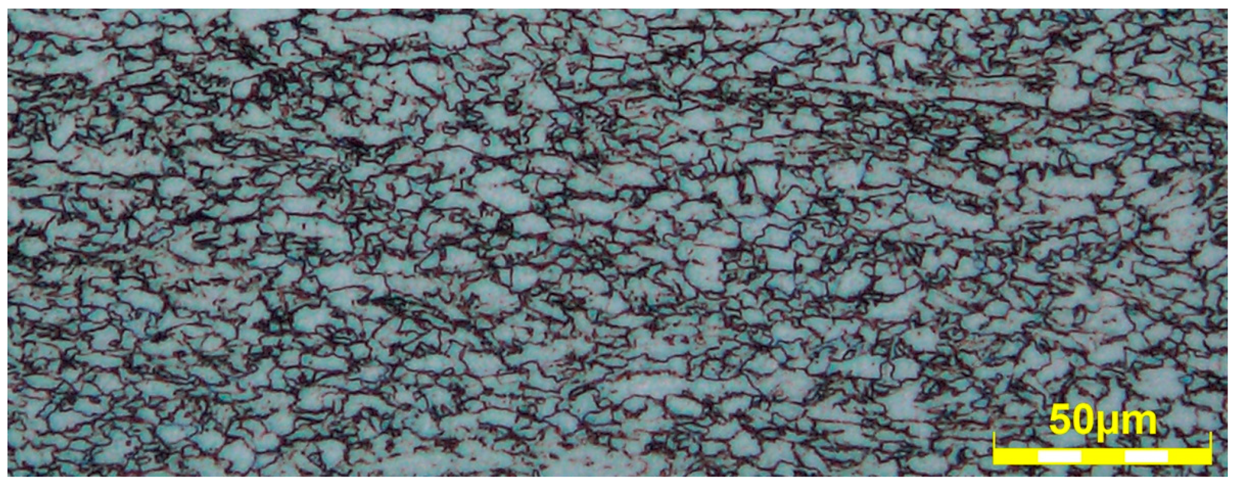
Figure 1.
Metallographic structure of the base material—steel S460MC.
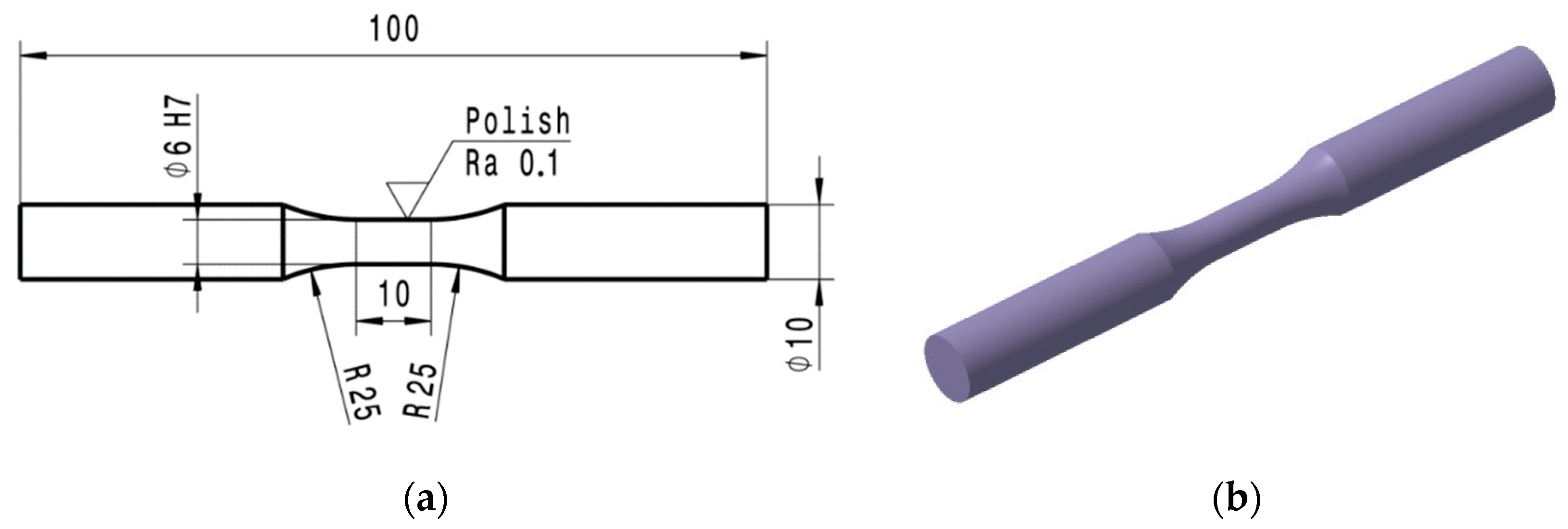
Figure 2.
(a) Dimensions and (b) 3D illustration of testing sample according to standard EN 3987. (unit: mm).
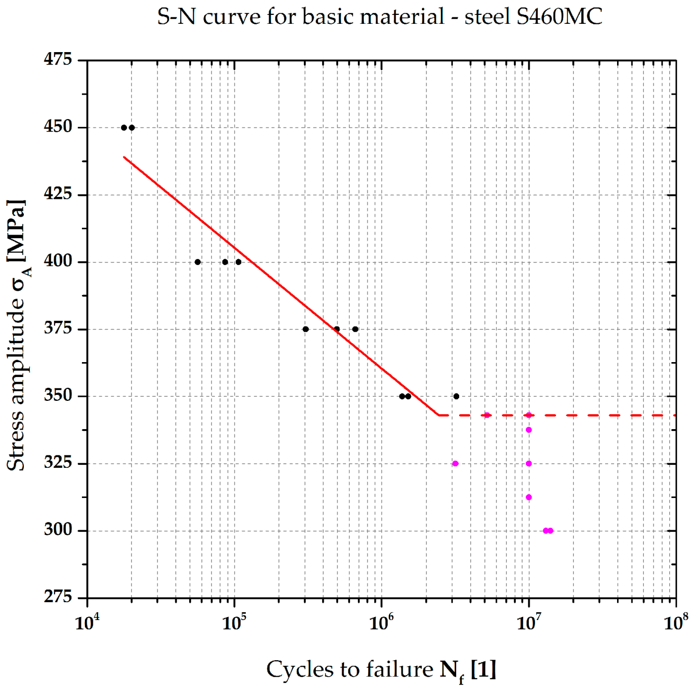
Figure 3.
S-N curve (semi-log scale) of the base material—steel S460MC.
Figure 4.
Measurement of the angular deformation after welding.
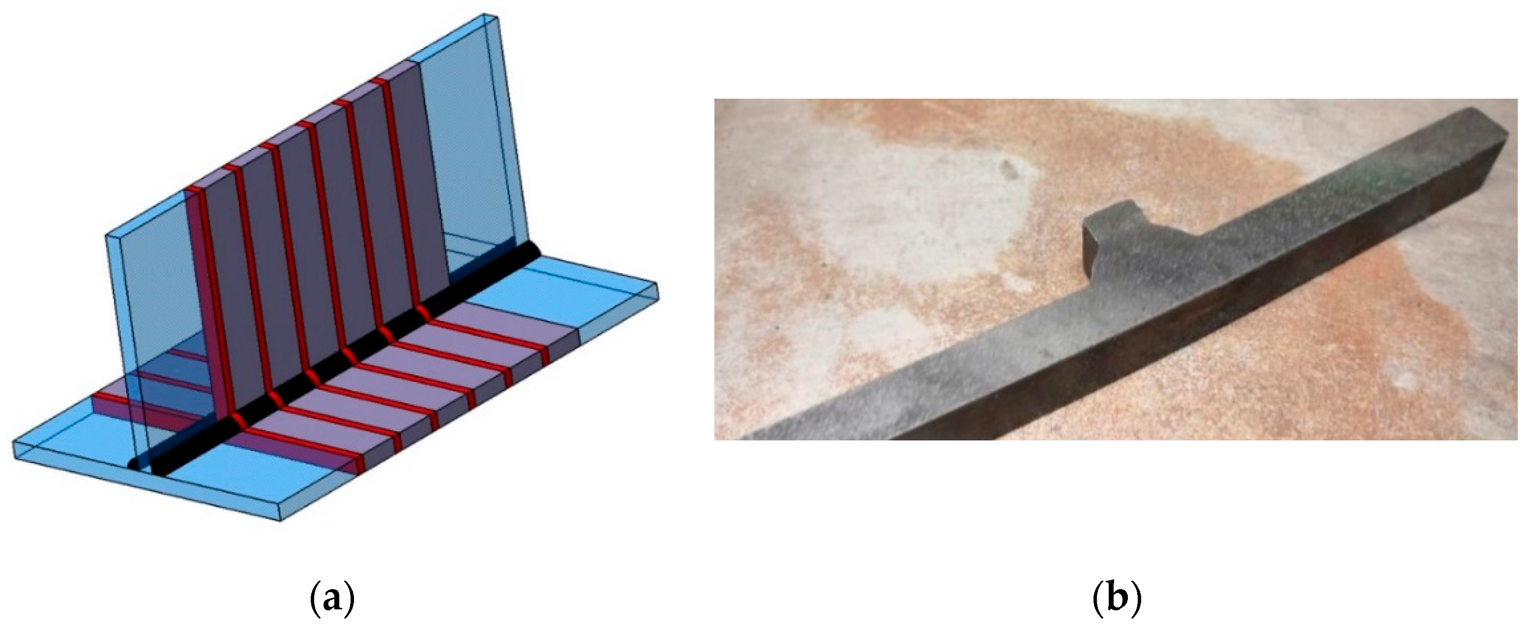
Figure 5.
Cyclic testing: (a) cutting of testing samples; (b) completely prepared testing sample.
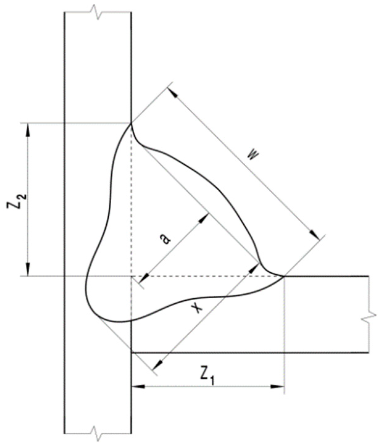
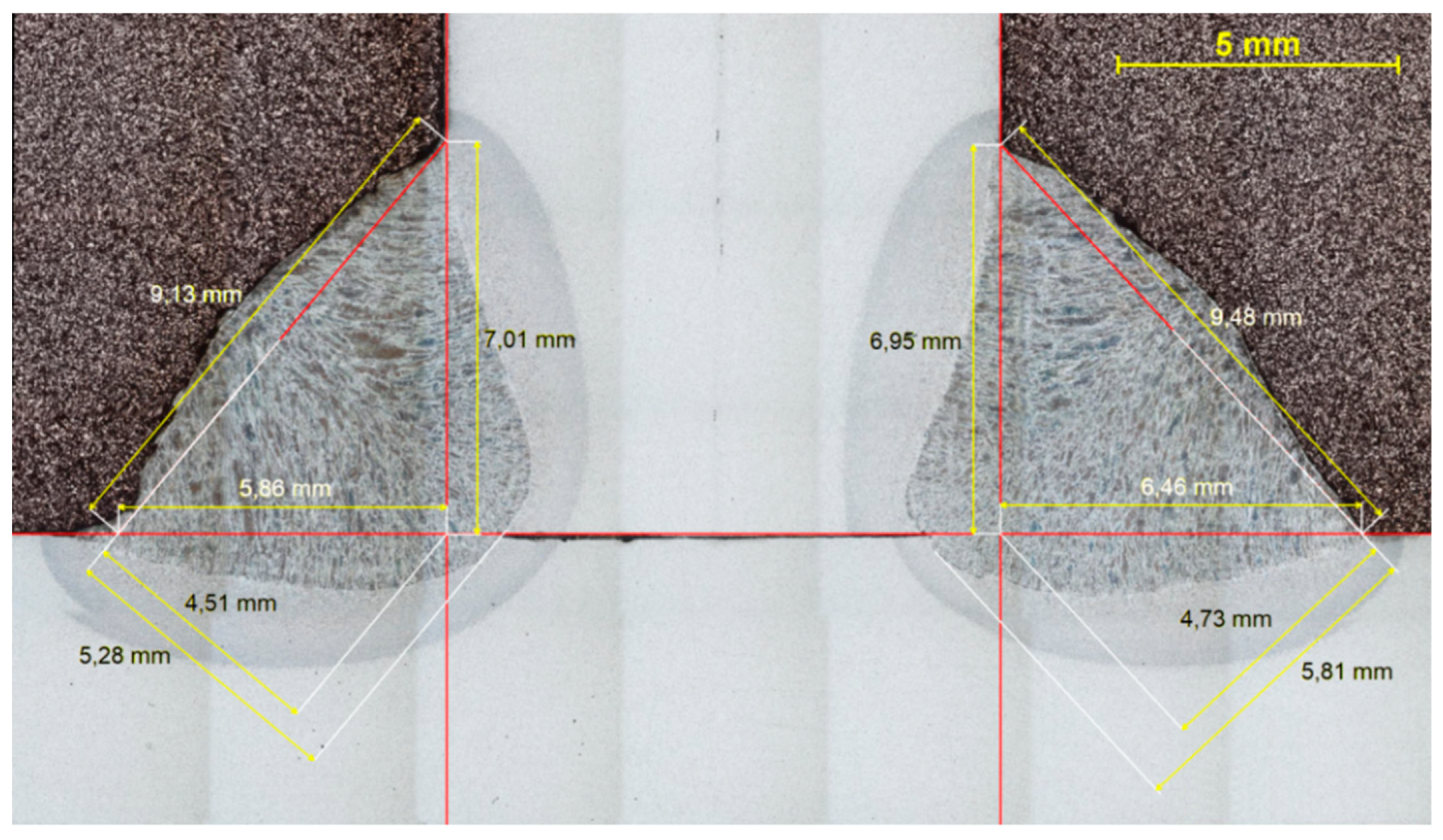
Figure 6.
Schematic illustration of the geometrically evaluated quantities of weld.
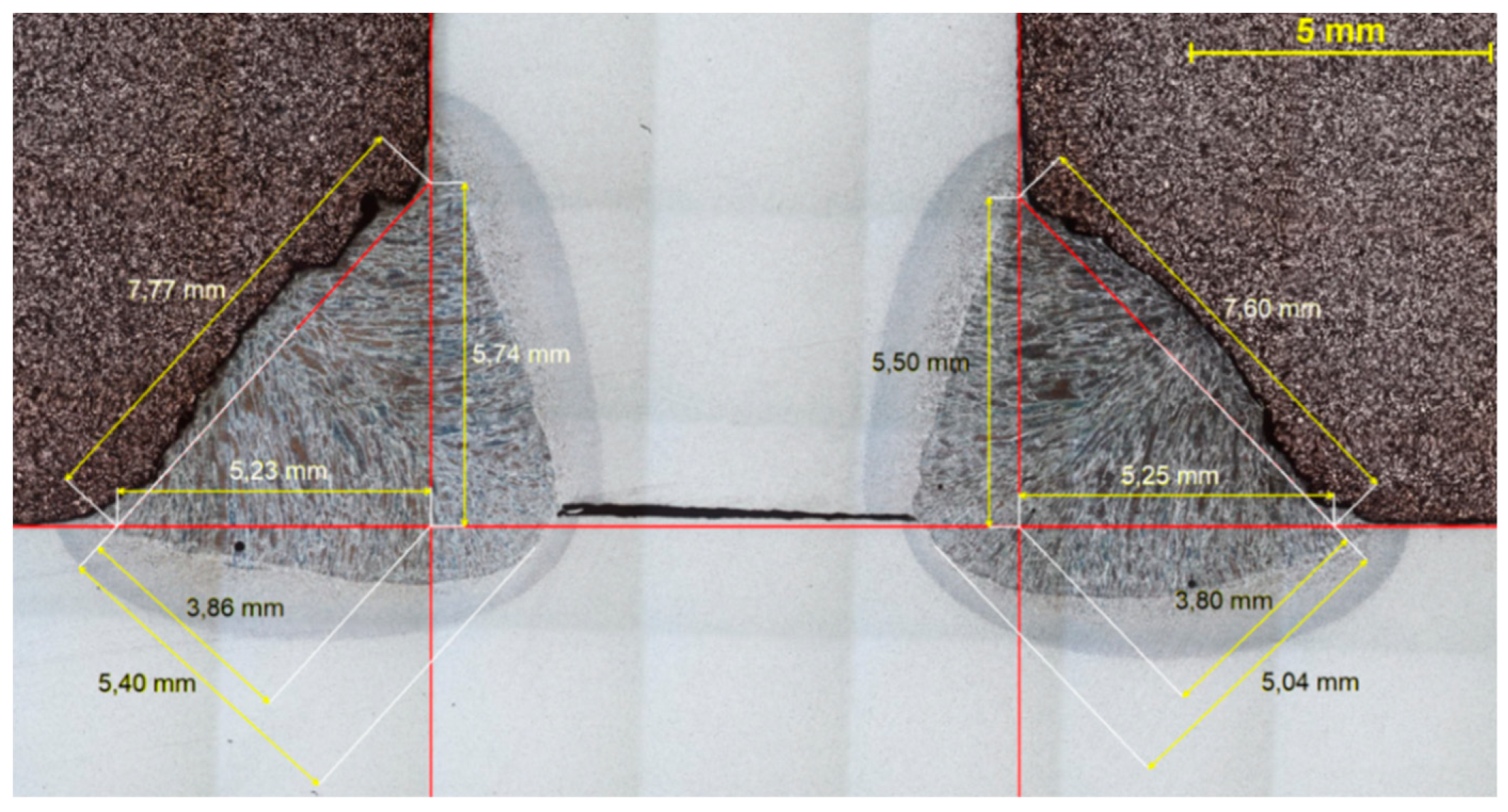
Figure 7.
Metallographic sample of Weld Q8 (Q = 8 kJ·cm−1)—1st bead (right) and 2nd bead (left).
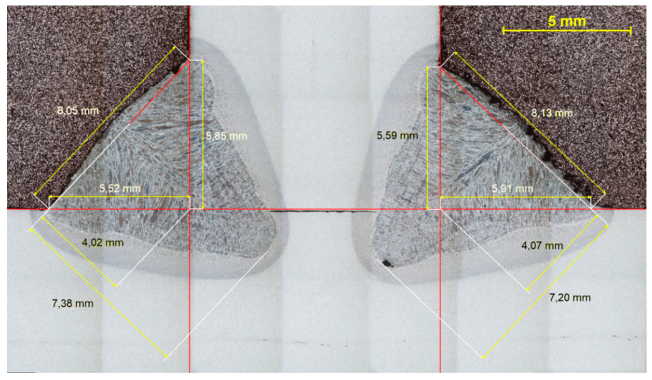
Figure 8.
Metallographic sample of Weld Q9 (Q = 9 kJ·cm−1)—1st bead (right) and 2nd bead (left).
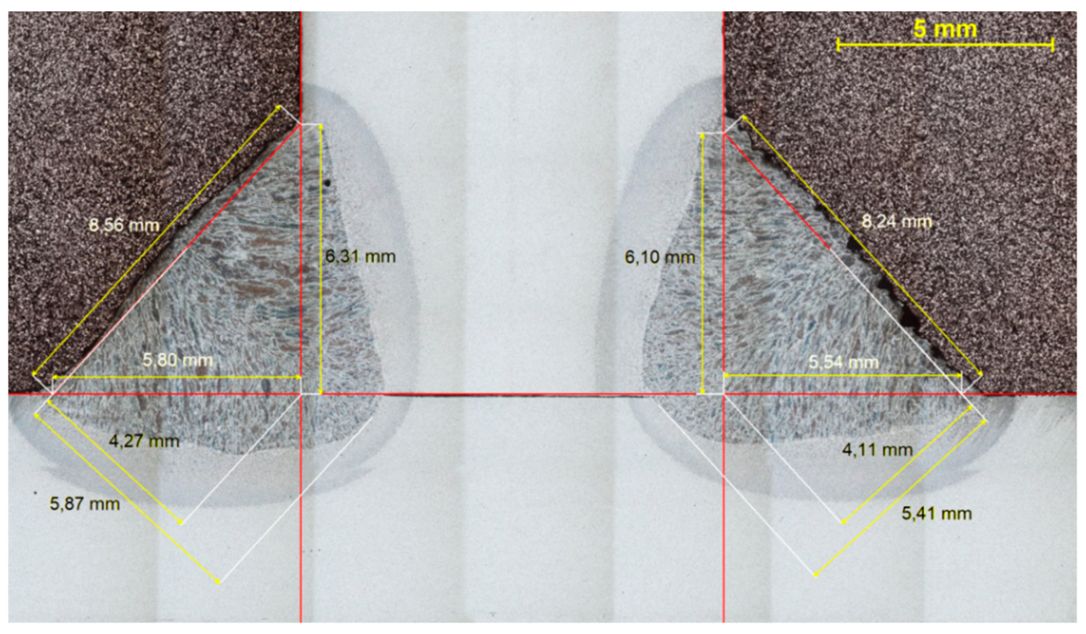
Figure 9.
Metallographic sample of Weld Q10 (Q = 10 kJ·cm−1)—1st bead (right) and 2nd bead (left).
Figure 10.
Metallographic sample of Weld Q12 (Q = 12 kJ·cm−1)—1st bead (right) and 2nd bead (left).
Figure 11.
Metallographic sample of Weld Q14 (Q = 14 kJ·cm−1)—1st bead (right) and 2nd bead (left).
Figure 12.
Shape adjustment and loading mode of fatigue tests.
Figure 13.
Location of crack initialization for Weld Q12: (a) σA = 300 MPa; (b) σA = 74 MPa.
Figure 14.
S-N curves (log-log scale)—graphical comparison of the measured trends (linear fitting according to Basquin’s equation) for fillet welds with different heat input values.
Table 1.
Chemical composition of the tested material—steel S460MC.
| Chemical Element | C | Mn | Si | P | S | Nb | W | Ni | V | Cr | Ti |
|---|
| Composition [wt %] | 0.07 | 1.32 | 0.01 | 0.03 | 0.01 | 0.05 | 0.04 | 0.04 | 0.08 | 0.01 | 0.01 |
Table 2.
Basic mechanical properties of tested material—steel S460MC.
| Mechanical Properties | Yield Strength
Re [MPa] | Ultimate Tensile Strength
Rm [MPa] | Uniform Ductility
Ag [%] | Total
Ductility
A30 [%] |
|---|
| EN 10149-2 | Min. 460 | 520–670 | X | Min. 17 |
| Measured values | 544 ± 17 | 629 ± 21 | 13.15 ± 0.42 | 29.03 ± 0.91 |
Table 3.
Process parameters adjusted on the power supply and linear automat.
| Weld Designation | Current
I [A] | Welding Speed
vs [m·min−1] | Expected Voltage
U [V] | Calculated Heat Input
Q [J·cm−1] |
|---|
| Weld Q8 | 260 | 0.505 | 26.0 | 8.03 |
| Weld Q9 | 320 | 0.600 | 28.1 | 8.99 |
| Weld Q10 | 260 | 0.400 | 25.7 | 10.02 |
| Weld Q12 | 250 | 0.300 | 23.9 | 11.95 |
| Weld Q14 | 265 | 0.295 | 26.0 | 14.01 |
Table 4.
Actual process parameters measured by the system WeldMonitor.
| Weld Designation | Number of Bead | Effective
Current
I [A] | Effective
Voltage
U [V] | Real Welding Speed
vs [m·min−1] | Heat Input
Q [J·cm−1] |
|---|
| Weld Q8 | 1 | 264.1 | 25.5 | 0.500 | 8.08 |
| 2 | 264.4 | 25.5 | 0.496 | 8.16 |
| Weld Q9 | 1 | 324.1 | 27.7 | 0.590 | 9.13 |
| 2 | 321.3 | 27.8 | 0.599 | 8.95 |
| Weld Q10 | 1 | 267.3 | 25.5 | 0.401 | 10.22 |
| 2 | 265.1 | 25.6 | 0.406 | 10.03 |
| Weld Q12 | 1 | 252.5 | 23.1 | 0.296 | 11.82 |
| 2 | 250.5 | 23.2 | 0.296 | 11.78 |
| Weld Q14 | 1 | 267.4 | 25.5 | 0.291 | 14.06 |
| 2 | 267.7 | 25.6 | 0.293 | 14.03 |
Table 5.
Magnitudes of the angular deformation for relevant welds.
| Bead/Weld | Weld Q8 | Weld Q9 | Weld Q10 | Weld Q12 | Weld Q14 |
|---|
| Bead 1 (P1) | 1.23 ± 0.17 | 1.43 ± 0.13 | 1.39 ± 0.11 | 1.41 ± 0.14 | 1.37 ± 0.14 |
| Bead 2 (P2) | 2.71 ± 0.15 | 3.21 ± 0.24 | 3.16 ± 0.18 | 3.18 ± 0.17 | 3.34 ± 0.26 |
Table 6.
Geometrical evaluation of the monitored weld beads.
| Weld Designation | Number of Bead | Measured Parameter [mm] |
|---|
| a | x | w | Z1 | Z2 | HAZf | HAZw | R |
|---|
|
Weld Q8
| 1 | 3.80 | 5.04 | 7.60 | 5.50 | 5.25 | 1.36 | 1.22 | 1.27 |
| 2 | 3.86 | 5.40 | 7.77 | 5.74 | 5.23 | 1.34 | 1.34 | 1.28 |
| Weld Q9 | 1 | 4.07 | 7.20 | 8.13 | 5.59 | 5.91 | 1.48 | 1.37 | 1.25 |
| 2 | 4.02 | 7.38 | 8.05 | 5.85 | 5.52 | 1.43 | 1.03 | 1.21 |
| Weld Q10 | 1 | 4.11 | 5.41 | 8.24 | 6.10 | 5.54 | 1.54 | 1.44 | 1.45 |
| 2 | 4.27 | 5.87 | 8.56 | 6.31 | 5.80 | 1.41 | 1.34 | 1.49 |
| Weld Q12 | 1 | 4.73 | 5.81 | 9.48 | 6.95 | 6.46 | 1.87 | 1.61 | 0.98 |
| 2 | 4.51 | 5.28 | 9.13 | 7.01 | 5.86 | 1.65 | 1.56 | 1.02 |
| Weld Q14 | 1 | 5.12 | 6.88 | 10.21 | 7.28 | 7.17 | 1.81 | 1.84 | 0.94 |
| 2 | 5.17 | 6.82 | 10.34 | 7.49 | 7.15 | 1.94 | 1.78 | 1.07 |
Table 7.
Cycles to failure Nf in dependence on stress amplitudes σA for the monitored welds.
Stress Amplitude
σA [MPa] | Cycles to Failure Nf [1] |
|---|
| Weld Q8 | Weld Q9 | Weld Q10 | Weld Q12 | Weld Q14 |
|---|
| 300 | 10,436 | 10,398 | 10,513 | 10,279 | 10,187 |
| 240 | 31,093 | 30,268 | 31,825 | 29,245 | 28,451 |
| 170 | 74,840 | 67,417 | 86,153 | 55,668 | 59,627 |
| 152.5 | 111,389 | 103,284 | 135,381 | 95,676 | 102,477 |
| 135 | 167,536 | 132,982 | 201,117 | 190,961 | 163,448 |
| 117.5 | 242,359 | 236,172 | 346,740 | 173,615 | 173,397 |
| 100 | 1,057,662 | 515,809 | 546,096 | 359,291 | 253,974 |
| 82.5 | 1,147,041 | 813,423 | 793,318 | 701,936 | 660,143 |
| 74 | 6,356,012 | 3,983,642 | 3,011,738 | 2,451,977 | 2,282,815 |
| 65 | >107 | >107 | >107 | >107 | >107 |
Table 8.
Values of fatigue strength coefficient σf and fatigue strength exponent b (computed according to Basquin’s equation) for the monitored fillet welds.
| Weld Designation | Average Heat Input
Q [kJ·cm−1] | Fatigue Strength Coefficient
σf [MPa] | Fatigue Strength Exponent
b [1] |
|---|
| Weld Q8 | 8.12 | 2715 ± 293 | −0.230 ± 0.020 |
| Weld Q9 | 9.04 | 3534 ± 359 | −0.255 ± 0.021 |
| Weld Q10 | 10.13 | 4427 ± 304 | −0.270 ± 0.015 |
| Weld Q12 | 11.80 | 4438 ± 419 | −0.276 ± 0.021 |
| Weld Q14 | 14.05 | 4704 ± 481 | −0.281 ± 0.023 |
© 2020 by the authors. Licensee MDPI, Basel, Switzerland. This article is an open access article distributed under the terms and conditions of the Creative Commons Attribution (CC BY) license (http://creativecommons.org/licenses/by/4.0/).


