Transient Flow–Thermal–Structural Response and Candidate High-Risk Region Identification of an Axial Piston Pump Slipper Pair Under Variable Loading

Abstract

In axial piston pumps under variable loading, the system-level excitation and local tribological responses of the slipper pair can become temporally and spatially decoupled. The scientific contribution of this paper is a phase-consistent chain that achieves three things: it resolves the central-pocket pressure boundary with a dual-orifice and dual-control-volume model instead of directly imposing piston chamber pressure, propagates this boundary through posture-dependent clearance to three-dimensional flow–thermal and single-slipper structural responses within the same local cycle, and screens candidate high-risk regions from the spatial proximity and phase relationship of multi-field cycle envelopes rather than from a single peak. The results show that the central pocket pressure exhibits peak attenuation, peak-time difference, and pressure-rate weakening relative to the piston chamber pressure. The steady peak attenuation ratio is $2.83$–$3.33\%$, while pressure-rate weakening under variable loading is $6.29$–$7.14\%$; the high-to-low unloading case gives the largest attenuation of $4.81\%$. Increasing steady load reduces the tilt amplitude and raises the minimum film thickness from about $13.024$ to $13.452\mathsf{\mu }\mathrm{m}$, but the maximum temperature rise increases from $34.12$ to $65.01\mathrm{K}$. A $10\%$ cycle-envelope projection shows no common overlap among the film-thinning, oil-film temperature-rise, and structural-stress core high-response regions with pairwise overlap ratios of 0–$3.27\%$. This traceable chain supports comparative lubrication-safety screening; the identified zones remain numerical candidates rather than experimentally confirmed wear or failure regions.

1. Introduction

Axial piston pumps are widely used in high-power hydraulic systems because of their high power density, compact structure, and flexible displacement regulation. As the operating pressure, rotational speed, and variable-load intensity increase, the slipper/swash-plate interface becomes a critical location where pressure pulsation, leakage, frictional heating, and local oil-film thinning may interact. The slipper pair is therefore not only a load-bearing friction pair but also a local multi-physics interface whose oil-film load carrying, leakage, temperature rise, and structural response affect pump efficiency and reliability. Early hydrostatic lubrication and slipper-geometry studies showed that the slipper oil film controls both support and leakage, and that its operating state depends on the pressure boundary, film thickness, posture, and sealing-land flow rather than on a single static pressure [1,2,3,4].

At the broader positive-displacement-pump level, Guan et al. combined theoretical modeling and experiments to characterize the leakage, delivered flow, power consumption, and noise of a spherical water pump prototype under multiple operating conditions [5]. For axial piston slipper pairs specifically, viscosity–temperature–pressure effects on leakage have also been examined [6].

Substantial progress has been made in modeling and measuring slipper-pair lubrication, posture evolution, and vibration–lubrication coupling. Theoretical models, finite-volume or computational fluid dynamics (CFD) calculations, and test-rig measurements have clarified that the slipper posture, oil-film thickness, pressure distribution, leakage, friction, and vibration response are strongly coupled [7,8,9,10,11]. These studies provide an important basis for describing the slipper pair beyond the idealized assumption of a parallel clearance. However, most available analyses still focus on steady or quasi-steady operating conditions. Under strong variable loading, the traceable path from system-level pressure excitation to local pressure boundary, instantaneous clearance, flow–thermal redistribution, and structural response remains insufficiently resolved.

For a swash-plate axial piston pump, the piston chamber pressure is not identical to the inlet pressure acting at the slipper bottom. The piston chamber pressure $p_{\mathrm{ct}}$ is transmitted through the piston damping orifice, transition chamber, slipper damping orifice, and central pocket before forming the actual local pressure boundary $p_{\mathrm{ht}}$. Studies on damping structures, porting processes, and AMESim-based flow characterization have shown that pressure signals are affected by orifice damping, chamber compressibility, cavitation, and leakage [12,13]. Therefore, directly imposing $p_{\mathrm{ct}}$ as the oil-film inlet pressure may overestimate pressure peaks, pressure-rate characteristics, and phase relations in downstream three-dimensional calculations.

Three-dimensional CFD and flow–thermal studies further show that posture-dependent clearance can modify pressure distribution, hydraulic lift, leakage, and temperature fields at the slipper/swash-plate interface [6,14,15,16,17]. Thermal and thermoelastohydrodynamic analyses also indicate that temperature-dependent viscosity, thermal deformation, and structural response influence the local lubrication state [18,19,20,21,22]. Meanwhile, mixed-lubrication and lubrication–wear interaction studies show that film thinning, temperature rise, asperity contact, and wear evolution are relevant to local service risk [23,24,25]. This paper does not introduce asperity contact, wear evolution, material yielding, or fatigue-life models. Consequently, the regions identified in this paper are defined as candidate high-risk regions rather than confirmed failure or wear regions.

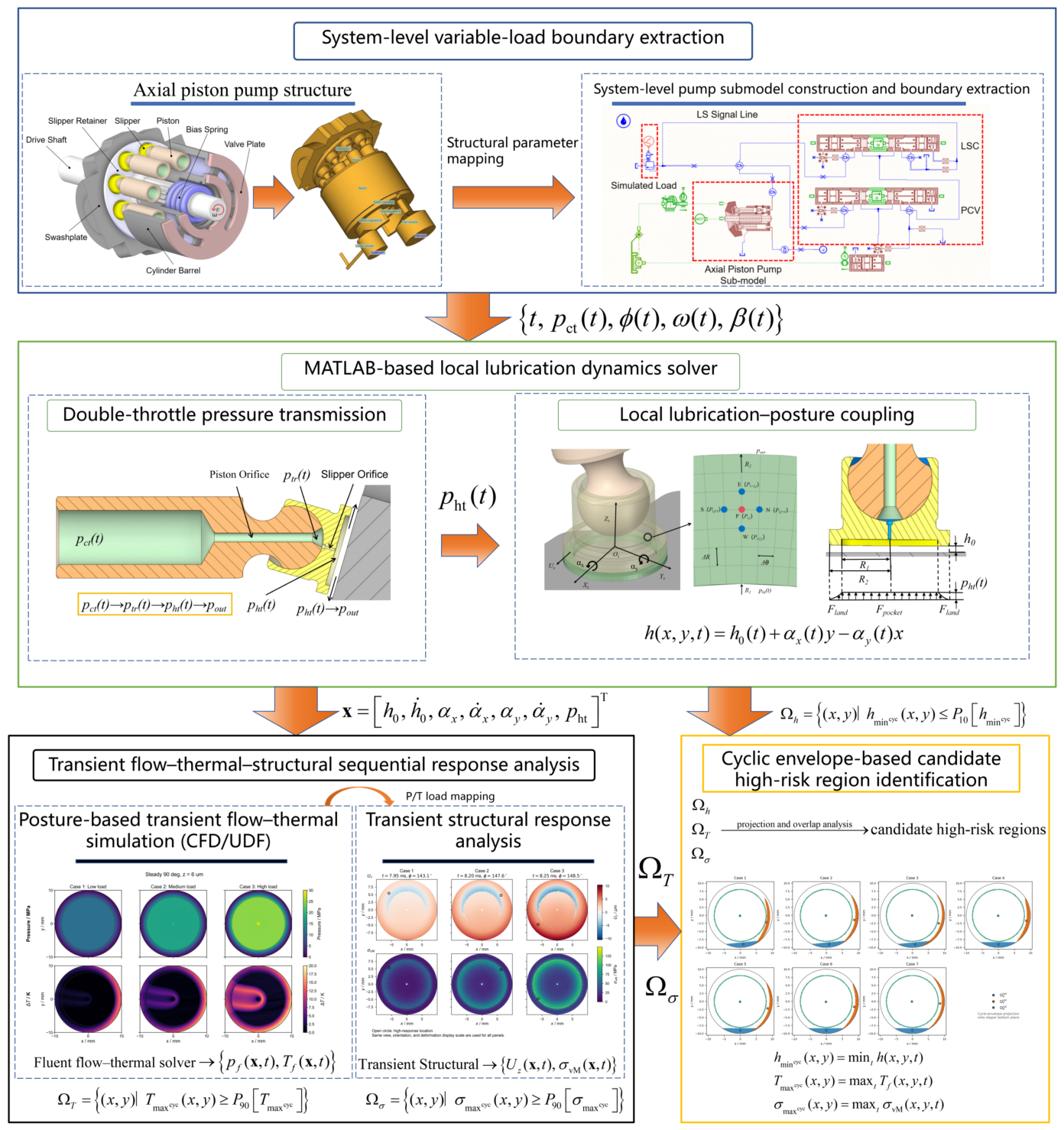
The unresolved problem is that existing studies rarely connect pressure-boundary correction, slipper posture evolution, posture-driven flow–thermal redistribution, and structural response into a single traceable chain under variable loading. In this paper, a flow–thermal–structural sequential coupling framework is established for a swash-plate axial piston pump slipper pair, as shown in Figure 1. The framework connects the cascade path of system-level piston chamber pressure → central pocket pressure → slipper posture → instantaneous clearance → three-dimensional flow–thermal field → single-slipper structural response → candidate high-risk region identification. The objective is to clarify how variable loading is transmitted through the pressure boundary and posture response, as well as how film-thinning, temperature-rise, and stress high-response regions become spatially adjacent within a cycle-envelope field.

2. Mathematical Model and Numerical Method

This section describes the computational chain used to transfer the variable-load excitation from the system model to the local lubrication, flow–thermal, and structural analyses. The method is organized into four modules: system-level boundary extraction, dual-orifice pressure transmission and slipper micro-motion lubrication, one-way flow–thermal–structural sequential coupling, and numerical reliability assessment. Detailed discretization formulae, interpolation expressions, and sensitivity tables are provided in Appendix A.

2.1. System-Level Variable-Load Boundary and Transient Excitation Extraction

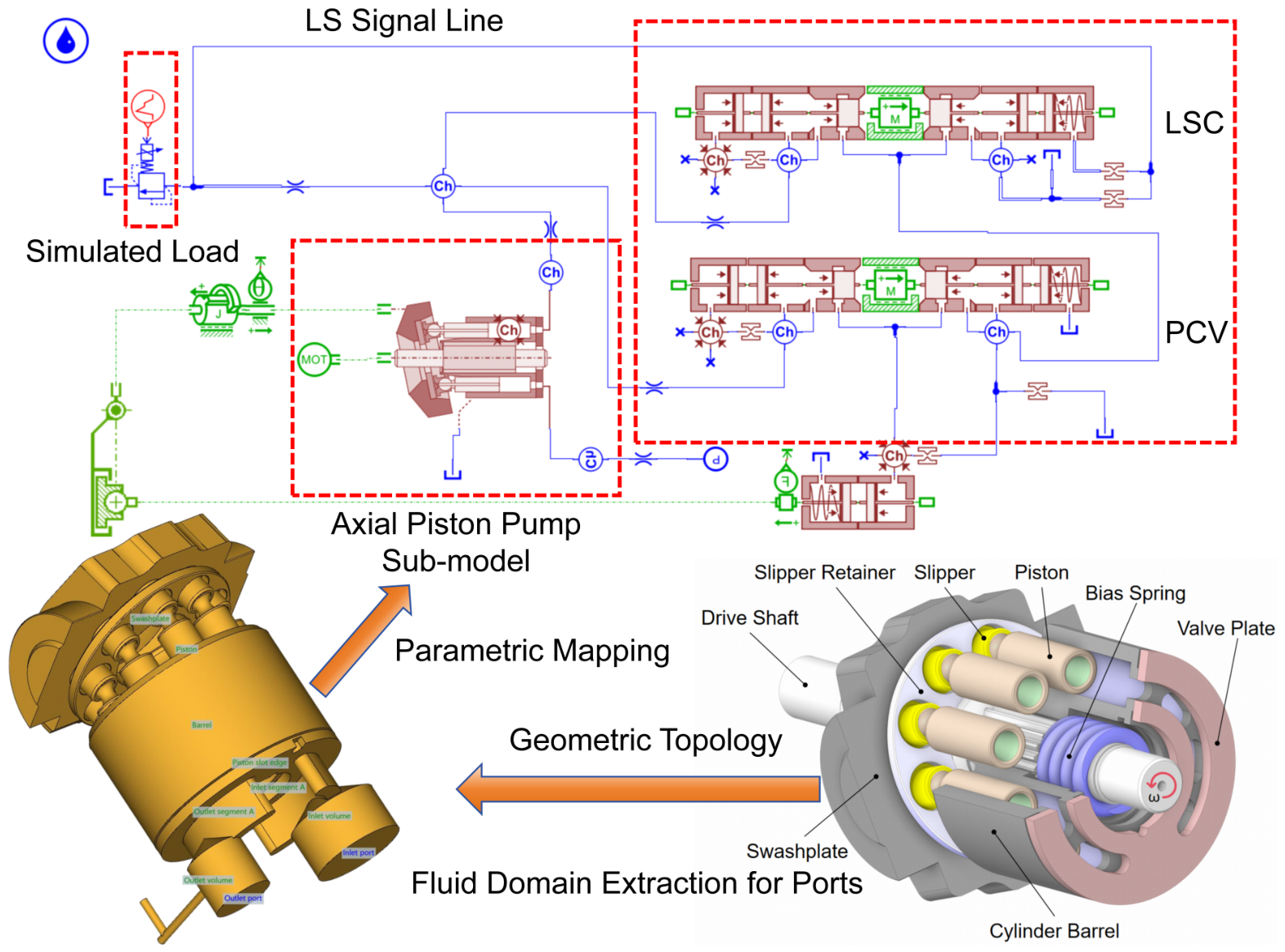
The system-level model shown in Figure 2 provides the piston chamber pressure and rigid-body phase information required by the local slipper-pair model. The exported variables are time t, piston chamber pressure $p_{\mathrm{ct}}\left(t\right)$, cylinder-block angle $\tilde{\varphi }\left(t\right)$, and swash-plate angle $\beta \left(t\right)$. The cylinder-block angle is unwrapped to remove artificial $0^{\circ }$–${360}^{\circ }$ jumps, and the relative phase and angular velocity are obtained as

$$\varphi \left(t\right)=unwrap\left[\tilde{\varphi }\left(t\right)\right]-unwrap\left[\tilde{\varphi }\left(0\right)\right],\omega \left(t\right)={\displaystyle \frac{\mathrm{d}\varphi \left(t\right)}{\mathrm{d}t}}.$$

(1)

Thus, the boundary vector transferred to the local lubrication model is $\{t,p_{\mathrm{ct}}\left(t\right),\varphi \left(t\right),\omega \left(t\right),$ $\beta \left(t\right)\}$. The pressure history drives the dual-orifice pressure-transmission model, whereas the phase and swash-plate angle determine the instantaneous motion state of the piston–slipper assembly.

The nominal rotational speed is $3000\mathrm{r}/\min$, corresponding to a rotation period of $0.02\mathrm{s}$. The global time window $t=0.20–0.22\mathrm{s}$ is therefore used as one complete comparison cycle. In the downstream flow–thermal, structural, and cycle-envelope calculations, this global window is converted to the local cycle time $t^{\prime }=0–20\mathrm{ms}$, where $t^{\prime }=t-0.20\mathrm{s}$. The seven operating cases are summarized in

Table 1. Operating conditions for steady and transient load cases.

Case	Condition	Target Pressure Level (MPa)	Purpose
Case 1	Low-load steady state	Low ($\sim 12.5$)	Steady baseline
Case 2	Medium-load steady state	Medium ($\sim 20.8$)	Steady baseline
Case 3	High-load steady state	High ($\sim 31.0$)	Steady baseline
Case 4	Low-to-medium	Medium ($\sim 20.8$)	Variable-load transition
Case 5	Medium-to-high	High ($\sim 31.0$)	Variable-load transition
Case 6	Low-to-high	High ($\sim 31.0$)	Large-amplitude loading
Case 7	High-to-low	Low ($\sim 12.5$)	Unloading transition

. Cases 1–3 are steady baselines at low, medium, and high load levels, whereas Cases 4–7 represent single-cycle variable-load paths.

The variable-load window is not interpreted as a small interval around a single step event. Instead, at $3000\mathrm{r}/\min$, it covers one complete rotation including suction, discharge, and load-transition phases. Therefore, subsequent comparisons are made on the basis of the cycle phase rather than a simplified single-step response.

2.2. Dual-Orifice and Dual-Control-Volume Pressure Transmission and Micro-Motion Lubrication Model

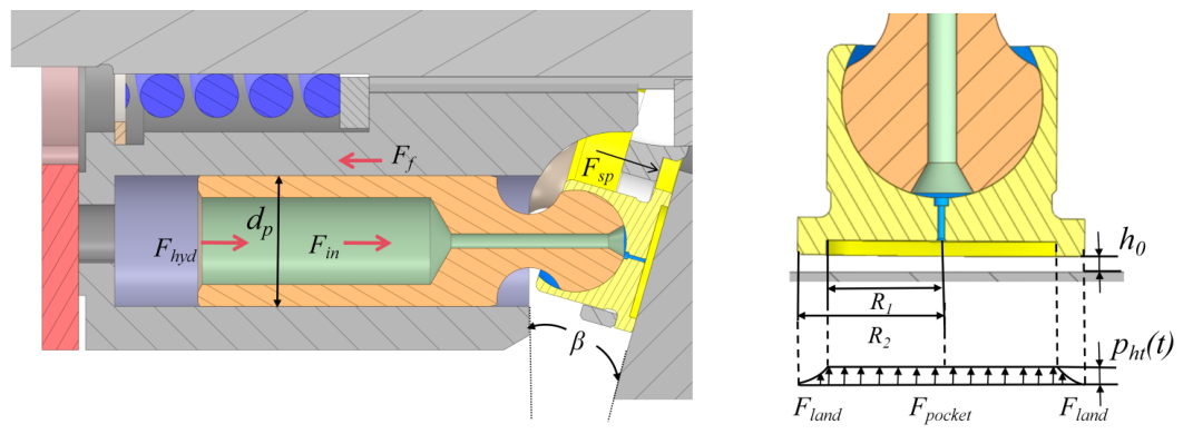
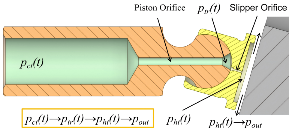
The piston chamber pressure is transmitted to the slipper bottom through the piston damping orifice, transition chamber, slipper damping orifice, and central pocket, as illustrated in Figure 3. The corresponding pressures are denoted by $p_{\mathrm{ct}}\left(t\right)$, $p_{\mathrm{tr}}\left(t\right)$, $p_{\mathrm{ht}}\left(t\right)$, and $p_{\mathrm{out}}$, respectively. Therefore, the pressure boundary acting on the slipper oil film is not the piston chamber pressure $p_{\mathrm{ct}}\left(t\right)$ directly but rather the central-pocket pressure $p_{\mathrm{ht}}\left(t\right)$ after dual-orifice and dual-control-volume modulation.

Both damping orifices are represented by an equivalent laminar conductance model,

$$G_i={\displaystyle \frac{\pi d_i^4}{128\mu L_i}},i=p,s,$$

(2)

where $d_i$ and $L_i$ are the diameter and length of the corresponding damping channel. The flow rates through the piston and slipper damping orifices are

$$Q_p=G_p[p_{\mathrm{ct}}\left(t\right)-p_{\mathrm{tr}}\left(t\right)],Q_s=G_s[p_{\mathrm{tr}}\left(t\right)-p_{\mathrm{ht}}\left(t\right)].$$

(3)

With oil bulk modulus K and chamber volumes $V_{\mathrm{tr}}$ and $V_{\mathrm{ht}}$, the pressure evolution is written as

$${\displaystyle \frac{\mathrm{d}{p}_{\mathrm{tr}}}{\mathrm{d}t}}={\displaystyle \frac{K}{V_{\mathrm{tr}}}}(Q_p-Q_s),{\displaystyle \frac{\mathrm{d}{p}_{\mathrm{ht}}}{\mathrm{d}t}}={\displaystyle \frac{K}{V_{\mathrm{ht}}}}(Q_s-Q_{\mathrm{leak}}-{\dot{V}}_{\mathrm{ht}}).$$

(4)

Here, $Q_{\mathrm{leak}}$ denotes radial leakage from the central pocket into the sealing-land annulus, and ${\dot{V}}_{\mathrm{ht}}$ denotes the equivalent volume-change rate induced by slipper micro-motion. Thus, $p_{\mathrm{ht}}\left(t\right)$ is a dynamically modulated local boundary rather than a direct copy of $p_{\mathrm{ct}}\left(t\right)$.

All pressures in this subsystem are gauge values, and the time-advancement scheme bounds $p_{\mathrm{tr}}$ and $p_{\mathrm{ht}}$ from below at $p_{\mathrm{out}}=0\mathrm{MPa}$ gauge. The formulation is single-phase and contains neither a gas/vapor volume-fraction state nor mass-transfer terms for dissolved-air release or vaporous cavitation; the lower-bound projection is therefore a numerical constraint rather than a cavitation model.

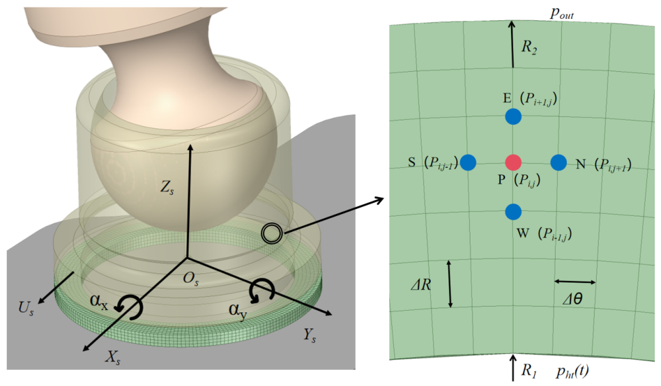
The slipper posture is described by the central film thickness $h_0\left(t\right)$ and the tilt components ${\alpha }_x\left(t\right)$ and ${\alpha }_y\left(t\right)$. In the local coordinate system at the slipper bottom, the instantaneous clearance is reconstructed as

$$h(x,y,t)=h_0\left(t\right)+{\alpha }_x\left(t\right)y-{\alpha }_y\left(t\right)x,$$

(5)

or, in polar coordinates,

$$h(r,\theta ,t)=h_0\left(t\right)+{\alpha }_x\left(t\right)rsin\theta -{\alpha }_y\left(t\right)rcos\theta ,h_{min}\left(t\right)=\underset{\mathsf{\Omega }}{min}h(r,\theta ,t).$$

(6)

This reconstruction links the overall normal displacement and two-dimensional tilt to the local film-thinning state. The corresponding geometry and polar discretization are shown in Figure 4.

The sealing-land oil film is modeled as a thin laminar Newtonian film. In the local translational coordinate system, the radial and circumferential velocity components are

$$u_r=U_x\left(t\right)cos\theta +U_y\left(t\right)sin\theta ,u_{\theta }=-U_x\left(t\right)sin\theta +U_y\left(t\right)cos\theta +\gamma \omega \left(t\right)r.$$

(7)

The transient Reynolds equation in polar coordinates is

$${\displaystyle \frac{1}{r}}{\displaystyle \frac{\partial }{\partial r}}\left(r{\displaystyle \frac{h^3}{12\mu }}{\displaystyle \frac{\partial p}{\partial r}}\right)+{\displaystyle \frac{1}{r^2}}{\displaystyle \frac{\partial }{\partial \theta }}\left({\displaystyle \frac{h^3}{12\mu }}{\displaystyle \frac{\partial p}{\partial \theta }}\right)={\displaystyle \frac{1}{2r}}{\displaystyle \frac{\partial \left(rh{u}_r\right)}{\partial r}}+{\displaystyle \frac{1}{2r}}{\displaystyle \frac{\partial \left(h{u}_{\theta }\right)}{\partial \theta }}+{\displaystyle \frac{\partial h}{\partial t}}.$$

(8)

The inner and outer radial pressure boundaries are $p(R_1,\theta ,t)=p_{\mathrm{ht}}\left(t\right)$ and $p(R_2,\theta ,t)=p_{\mathrm{out}}$, respectively, with circumferential periodicity and Reynolds-type pressure truncation for non-physical negative pressure. The force-balance and hydrostatic-support decomposition used in the model is shown in Figure 5.

The oil-film support force, anti-overturning moments, and leakage flux are obtained from the solved pressure field:

$$F_{\mathrm{land}}={\int \int }_{\mathsf{\Omega }}[p(r,\theta ,t)-p_{\mathrm{out}}]\mathrm{d}A,F_{\mathrm{pocket}}=[p_{\mathrm{ht}}\left(t\right)-p_{\mathrm{out}}]A_{\mathrm{ht}},$$

(9)

$$M_{x,\mathrm{film}}={\int \int }_{\mathsf{\Omega }}[p(r,\theta ,t)-p_{\mathrm{out}}]y\mathrm{d}A,M_{y,\mathrm{film}}=-{\int \int }_{\mathsf{\Omega }}[p(r,\theta ,t)-p_{\mathrm{out}}]x\mathrm{d}A,$$

(10)

$$Q_{\mathrm{leak}}={\int }_0^{2\pi }{\left[-{\displaystyle \frac{h^3}{12\mu }}{\displaystyle \frac{\partial p}{\partial r}}+{\displaystyle \frac{1}{2}}h{u}_r\right]}_{r=R_1}{R}_1\mathrm{d}\theta .$$

(11)

The posture variables are updated by reducing the normal force residual and the two overturning-moment residuals. The detailed state-space form and successive over-relaxation (SOR) discretization are provided in Appendix A.

2.3. Flow–Thermal–Structural Sequential Coupling Method

The sequential coupling strategy follows a one-way data-transfer topology: system-level dynamics (AMESim) → local lubrication and instantaneous posture solution (MATLAB R2024a) → three-dimensional transient flow–thermal reconstruction (Fluent) → solid heat conduction (Transient Thermal) → structural thermal–mechanical response (Transient Structural). The Fluent pressure field is transferred directly to the structural model, whereas the Fluent temperature field first passes through the transient thermal model. Unlike fully coupled thermoelastohydrodynamic (TEHD) or thermo-mechanical models [21,22], the present framework neither returns the solid-side interfacial heat flux to Fluent nor feeds the fluid-domain thermal or structural response back to modify the macroscopic rigid-body posture. This choice is consistent with the objective of tracing the forward transfer of variable-load excitation and avoids repeated cross-scale mesh reconstruction.

In the flow–thermal calculation, the comparison window is shifted to the local time $t^{\prime }=t-t_0$, and the central pocket pressure is imposed as

$$p_{\mathrm{in}}\left(t^{\prime }\right)=p_{\mathrm{ht}}(t_0+t^{\prime }).$$

(12)

The slipper wall is treated as a rigid moving boundary driven by the posture history with lifting and angular velocities obtained from $h_0\left(t\right)$, ${\alpha }_x\left(t\right)$, and ${\alpha }_y\left(t\right)$. When the solver time step is not exactly aligned with the MATLAB sampling points, the pressure and posture histories are synchronized by the same linear interpolation rule, which is given in Appendix A.

The oil in the three-dimensional flow–thermal field is treated as an incompressible Newtonian fluid with pressure- and temperature-dependent viscosity. The governing equations are

$$\nabla ·\mathbf{u}=0,$$

(13)

$$\rho \left({\displaystyle \frac{\partial \mathbf{u}}{\partial t}}+\mathbf{u}·\nabla \mathbf{u}\right)=-\nabla p+\nabla ·\left[{\mu }_f(p_g,T)(\nabla \mathbf{u}+\nabla {\mathbf{u}}^{\mathrm{T}})\right],$$

(14)

$$\rho c_p\left({\displaystyle \frac{\partial T}{\partial t}}+\mathbf{u}·\nabla T\right)=\nabla ·(k_f\nabla T)+\Phi ,\Phi =\tau :\nabla \mathbf{u}.$$

(15)

For No. 10 aviation hydraulic oil, $\rho =850\mathrm{kg}/{\mathrm{m}}^3$, $c_p=2040\mathrm{J}/(\mathrm{kg}·\mathrm{K})$, and $k_f=0.12\mathrm{W}/(\mathrm{m}·\mathrm{K})$ are used according to Li et al. [26]. In the present calculations, these three thermophysical properties are treated as constants independent of pressure and temperature; among the oil properties listed in

Table A1. Oil physical properties and viscosity-model parameters.

Parameter	Symbol	Value	Unit	Source Type
Constant physical properties
Density	$\rho$	850	kg/m3	source-data table
Specific heat capacity	$c_p$	2040	J/(kg·K)	source-data table
Thermal conductivity	$k_f$	0.12	W/(m·K)	source-data table
MATLAB constant viscosity	${\mu }_{\mathrm{MATLAB}}$	0.0168	Pa·s	MATLAB posture model
Fluent separable Barus–Reynolds viscosity model
Reference viscosity	${\mu }_{\mathrm{ref}}$	0.013099	Pa·s	Fluent material expression
Reference temperature	$T_{\mathrm{ref},\mu }$	303.15	K	Fluent material expression
Temperature–viscosity coefficient	${\lambda }_T$	0.0173	K−1	Fluent material expression
Pressure–viscosity coefficient	$a_p$	$2.3\times {10}^{-8}$	Pa−1	Fluent material expression
Viscosity lower/upper bounds	${\mu }_{min},{\mu }_{max}$	0.002/0.05	Pa·s	Fluent material expression
Inlet/reference temperature	$T_{\mathrm{in}}$	300	K	Fluent boundary/setup
Atmospheric-pressure viscosity–temperature data
Viscosity at 20 °C	${\mu }_{20}$	0.016812	Pa·s	source-data table
Viscosity at 30 °C	${\mu }_{30}$	0.013099	Pa·s	source-data table
Viscosity at 40 °C	${\mu }_{40}$	0.010425	Pa·s	source-data table
Viscosity at 50 °C	${\mu }_{50}$	0.008785	Pa·s	source-data table
Viscosity at 60 °C	${\mu }_{60}$	0.007385	Pa·s	source-data table
Viscosity at 70 °C	${\mu }_{70}$	0.006303	Pa·s	source-data table
Viscosity at 80 °C	${\mu }_{80}$	0.005408	Pa·s	source-data table
Viscosity at 90 °C	${\mu }_{90}$	0.004614	Pa·s	source-data table
Viscosity at 100 °C	${\mu }_{100}$	0.004012	Pa·s	source-data table
Viscosity at 110 °C	${\mu }_{110}$	0.003528	Pa·s	source-data table
Viscosity at 120 °C	${\mu }_{120}$	0.002760	Pa·s	source-data table

, only the Fluent dynamic viscosity varies with both variables through the relation below. The viscosity–temperature data are listed in Table A1. The Barus–Reynolds viscosity model is

$${\mu }_f(p_g,T)={\mu }_{\mathrm{ref}}exp\left[a_p{p}_g-{\lambda }_T(T-T_{\mathrm{ref}})\right],$$

(16)

where $T_{\mathrm{ref}}=303.15\mathrm{K}$, ${\mu }_{\mathrm{ref}}=0.013099\mathrm{Pa}·\mathrm{s}$, ${\lambda }_T=0.0173{\mathrm{K}}^{-1}$, and $a_p=2.3\times {10}^{-8}{\mathrm{Pa}}^{-1}$.

The separable Barus–Reynolds form was retained as a bounded engineering approximation rather than being treated as universally superior to the Roelands model. The available No. 10 aviation-hydraulic-oil data comprise 11 atmospheric-pressure viscosity values over 20–120 °C; the implemented temperature term reproduces these values with $R^2=0.987$ and a mean absolute percentage error of $3.67\%$. The imposed and computed pressures do not exceed approximately $31.0\mathrm{MPa}$, and the maximum fluid temperature is approximately $365.0\mathrm{K}$. Roelands-type correlations are more flexible when lubricant-specific high-pressure rheological data are available and have been used in detailed TEHD slipper modeling [21,27]. However, the present source package contains neither oil-specific Roelands parameters nor a high-pressure viscosity curve for No. 10 oil. Introducing generic Roelands parameters would therefore add an unverified assumption rather than improve parameter traceability.

In Fluent, the two oil-facing moving-wall zones were assigned zero normal heat flux, $q_n=0$. This is a fluid-side thermal simplification and does not imply that the ZQSn10-1 bronze slipper is non-conducting. After the Fluent calculation, the temperature histories on the pocket and sealing-land surfaces were mapped as two prescribed-temperature loads to a separate transient thermal model of the slipper. Transient heat conduction was then solved using the bronze thermal properties, and the resulting solid-temperature field was transferred to the transient structural model, while the Fluent pressure field was mapped directly as surface traction. Because the resulting solid-side heat flux was not returned to Fluent, the procedure remains a one-way sequential coupling rather than a conjugate fluid–solid heat-transfer solution.

Using the properties in

Table A6. Transient thermal and structural solver settings.

Parameter	Symbol	Value	Unit	Source Type
Material
Material	–	ZQSn10-1 tin bronze	–	Structural setup
Young’s modulus	E	110	GPa	Structural setup
Poisson’s ratio	$\nu$	0.33	–	Structural setup
Density	${\rho }_s$	8770	kg/m3	Structural setup
Thermal expansion coefficient	${\alpha }_T$	$1.76\times {10}^{-5}$	K−1	Structural setup
Thermal conductivity	$k_s$	71	W/(m·K)	Structural setup
Specific heat	$c_s$	396.1	J/(kg·K)	Structural setup
Model and mesh
Structural body	–	single slipper	–	Structural setup
Contact pair	–	not included	–	Structural setup
Formal mesh nodes	–	$4.942\times {10}^5$	–	Structural setup
Formal mesh elements	–	$3.548\times {10}^5$	–	Structural setup
Element type	–	SOLID187, 10-node quadratic tetrahedron	–	Structural setup
Coarse mesh nodes/elements	–	352275/253394	–	Structural setup
Fine mesh nodes/elements	–	660612/474232	–	Structural setup
Constraints
Support type	–	remote displacement, ball-joint equivalent	–	Structural setup
Remote point	–	slipper-bottom geometric center	–	Structural setup
X displacement	$U_X$	0	m	Structural setup
Y displacement	$U_Y$	0	m	Structural setup
Z displacement	$U_Z$	$z\left(t^{\prime }\right)$	m	From MATLAB posture
X rotation	$R_X$	${\theta }_x\left(t^{\prime }\right)$	rad	From MATLAB posture
Y rotation	$R_Y$	${\theta }_y\left(t^{\prime }\right)$	rad	From MATLAB posture
Z rotation	$R_Z$	0	rad	Structural setup
Thermal transfer, loads, and outputs
Initial solid temperature	–	300	K	Transient Thermal setup
CFD-to-thermal load	–	mapped oil-film temperature histories	K	From Fluent temperature field
CFD-to-thermal load scope	–	pocket and sealing-land oil-facing surfaces	–	two imported-temperature loads
Solid thermal solution	–	transient conduction in one ZQSn10-1 slipper body	–	Transient Thermal setup
Thermal-to-structural load	–	calculated solid-temperature field	K	From Transient Thermal solution
Pressure load	–	mapped oil-film pressure field	Pa	From Fluent pressure field
Pressure direction	–	${\mathbf{t}}_p=-p\mathbf{n}$	–	Structural setup
Thermal/structural time step	$\mathsf{\Delta }{t}_{\mathrm{struct}}$	$5.0\times {10}^{-5}$	s	Transient Thermal/Structural setup
Total simulation time	–	0.02	s	Structural setup
Number of output steps	–	400	–	Structural setup
Output quantities	–	$U_{\mathrm{total}},U_z,{\sigma }_{\mathrm{vM}},T_{max}$	–	Post-processing definition

, the bronze thermal diffusivity is ${\alpha }_s=k_s/\left({\rho }_s{c}_s\right)=2.04\times {10}^{-5}{\mathrm{m}}^2/\mathrm{s}$. The corresponding characteristic diffusion length is $\sqrt{{\alpha }_{s}t}=0.19\mathrm{mm}$ at the Case 7 fluid-temperature peak time of $1.75\mathrm{ms}$ and approximately $0.64\mathrm{mm}$ over the full $20\mathrm{ms}$ local cycle. Thus, local conduction in the bronze is physically relevant within the analyzed window; the zero-flux Fluent condition should be interpreted only as the fluid-side boundary used in the present sequential model.

The transient structural model receives the same-source posture boundary, the pressure field exported from Fluent, and the solid-temperature field calculated by the intervening transient thermal model. The posture boundary is imposed through relative increments with respect to the zero-time state,

$$z\left(t^{\prime }\right)=h_0(t_0+t^{\prime })-h_0\left(t_0\right),{\theta }_x\left(t^{\prime }\right)={\alpha }_x(t_0+t^{\prime })-{\alpha }_x\left(t_0\right),{\theta }_y\left(t^{\prime }\right)={\alpha }_y(t_0+t^{\prime })-{\alpha }_y\left(t_0\right).$$

(17)

The pressure field is mapped as a normal traction, ${\mathbf{t}}_p(\mathbf{x},t^{\prime })=-p(\mathbf{x},t^{\prime })\mathbf{n}$, and the calculated solid-temperature field is imported as a thermal load. For an isotropic solid, the thermal strain is

$${\epsilon }_{\mathrm{th}}={\alpha }_T[T(\mathbf{x},t^{\prime })-T_{\mathrm{ref}}]\mathbf{I}.$$

(18)

The structural model contains a single slipper body only. No slipper–swash-plate contact pair, asperity contact, wear evolution, material yielding, or fatigue-life criterion is introduced.

2.4. Numerical Implementation and Model Reliability Assessment

The MATLAB lubrication model uses a polar annular grid with $n_r=25$ radial nodes and $n_{\theta }=72$ circumferential nodes. Each system-level case lasts approximately $1.0\mathrm{s}$ and contains approximately 20,000 sampling points, corresponding to an average interval of $\mathsf{\Delta }t\approx 5.0\times {10}^{-5}\mathrm{s}$. The Reynolds pressure field is solved using a pointwise SOR method with relaxation factor ${\omega }_{\mathrm{SOR}}=1.6$, pressure residual threshold $20\mathrm{Pa}$, and maximum iteration number 200. The value ${\omega }_{\mathrm{SOR}}=1.6$ is retained as an empirically robust setting rather than a theoretical spectral-radius optimum. In a full-trace sweep over representative Cases 2, 6, and 7, all 240,000 pressure solves converged; relative to 1.6, a value of 1.55 reduced the total iteration count by only $0.038\%$, whereas 1.65 and 1.70 increased it by $0.017\%$ and $0.063\%$, respectively (

Table A12. SOR relaxation-factor sensitivity for representative Cases 2, 6, and 7 on the formal $25\times 72$ grid.

${\mathit{\omega }}_{\mathbf{SOR}}$	Conv./Total	Total Iter.	Mean Iter.	P95	Max. Iter.	Max. Residual (Pa)	Max. Change (%)
1.55	60,000/60,000	60,075	1.001250	1	2	19.961	0.595
1.60	60,000/60,000	60,098	1.001633	1	2	19.935	–
1.65	60,000/60,000	60,108	1.001800	1	2	19.947	1.331
1.70	60,000/60,000	60,136	1.002267	1	2	19.968	1.201

Note: P95 denotes the 95th percentile of the iteration count per pressure solve. Each row aggregates 60,000 time steps from the three cases. The maximum output change is the largest absolute relative difference in pocket-pressure peak, minimum film thickness, maximum tilt magnitude, mean leakage, or leakage integral relative to ω_SOR = 1.60.

). To avoid non-physical thin-film states, $h_{min,\lim }=0.30\mathsf{\mu }\mathrm{m}$, $h_{0,max}=40\mathsf{\mu }\mathrm{m}$, and ${\left|\alpha \right|}_{max}=1000\mathsf{\mu }\mathrm{rad}$ are used.

Discretization reliability was evaluated at three levels. For the MATLAB lubrication solver, refinement from the formal $25\times 72$ polar grid to a $33\times 96$ reference grid produced a maximum relative deviation of $2.68\%$ for the principal pressure, posture, and leakage indicators, whereas halving the input time step produced a maximum relative deviation of $1.31\%$. For the three-dimensional flow–thermal calculation, Case 7 was selected as a representative high-to-low unloading condition. The maximum relative deviations in the grid and time-step sensitivity checks were $5.393\%$ and $3.715\%$, respectively, and the dominant hydraulic indicators showed much smaller deviations. For the transient structural model, the formal structural mesh yielded a window-averaged equivalent-stress error of $1.249\%$ and a window-averaged maximum-deformation error of $0.148\%$ relative to the fine mesh. The full sensitivity tables are provided as

Table A8. Fluent grid sensitivity analysis for Case 7.

Metric	Test	Ref.	End Err. (%)	Peak Err. (%)
$F_{\mathrm{lift}}$ (N)	−2740.668	−2741.200	0.019	0.083
${\dot{m}}_{\mathrm{in}}$ (kg/s)	0.013284	0.013292	0.058	0.161
${\dot{m}}_{\mathrm{out}}$ (kg/s)	−0.013284	−0.013292	0.066	0.171
${\overline{\mathsf{\Delta }T}}_{f,\mathrm{mean}}$ (K)	0.555	0.580	4.271	5.393
$\mathsf{\Delta }{T}_{max}$ (K)	26.988	27.455	1.701	1.704

Note: “Test” denotes the grid solution being evaluated, whereas “Ref.” denotes the reference grid solution. The end error is calculated from the final or window-averaged value, and the peak error is calculated from the peak or time-series response.

,

Table A9. Fluent time-step sensitivity analysis for Case 7.

Metric	Test	Ref.	End Err. (%)	Peak Err. (%)
$F_{\mathrm{lift}}$ (N)	−5248.430	−5248.184	0.005	0.030
${\dot{m}}_{\mathrm{in}}$ (kg/s)	0.028279	0.028282	0.010	0.018
${\dot{m}}_{\mathrm{out}}$ (kg/s)	−0.028280	−0.028283	0.010	0.019
${\overline{\mathsf{\Delta }T}}_{f,\mathrm{mean}}$ (K)	1.732	1.670	3.715	0.564
$\mathsf{\Delta }{T}_{max}$ (K)	51.732	50.400	2.642	0.197

Note: “Test” denotes the time-step solution being evaluated, whereas “Ref.” denotes the reference time-step solution. The end error is calculated from the final or window-averaged value, and the peak error is calculated from the peak or time-series response.

and

Table A10. Structural grid sensitivity analysis for Case 7.

Mesh	${\overline{\mathit{\sigma }}}_{\mathbf{vM},\mathit{R}}$ (MPa)	${\overline{\mathit{d}}}_{max}$ ($\mathsf{\mu }$m)	${\mathit{e}}_{\mathit{\sigma }}$ (%)	${\mathit{e}}_{\mathit{d}}$ (%)
Coarse mesh	32.605	7.582	4.063	0.452
Formal mesh	33.562	7.605	1.249	0.148
Fine mesh	33.986	7.616	–	–

Note: The relative errors $e_{\sigma }$ and $e_d$ are calculated with respect to the fine-mesh solution.

in Appendix A. Mesh quality was additionally audited for all three CFD and structural mesh levels. Fluent-native statistics were extracted for the setup mesh and every archived dynamic-mesh state (126 states in total), whereas the SOLID187 volume elements were assessed using corner-node element quality and skewness together with Ansys Mechanical APDL (MAPDL; APDL denotes Ansys Parametric Design Language)-native aspect-ratio and Jacobian-ratio checks. The worst-case statistics and structural outlier context are reported in

Table A13. Mesh-quality statistics for the three CFD and structural mesh levels.

(a) Fluent CFD meshes: worst statistics over the archived dynamic-mesh states.
Mesh	States	Cells	Nodes	Min. OQ	Mean/Max. Skew.	Mean/Max. AR
Coarse	22	1,808,243	1,934,256	0.309	0.055/0.691	10.505/38.269
Formal	82	2,918,073	3,067,526	0.309	0.054/0.691	7.386/38.269
Fine	22	4,360,852	4,540,777	0.309	0.054/0.691	6.387/38.269
(b) Mechanical structural meshes: SOLID187 volume-element statistics.
Mesh	Nodes	Elements	SOLID187	Mean/Min. EQ	Mean/Max. Skew.	Mean/Max. AR	Mean/Max. JR
Coarse	352,275	253,394	228,701	0.810/0.143	0.277/0.947	1.941/14.570	1.005/3.708
Formal	494,222	354,839	324,722	0.815/0.153	0.268/0.963	1.921/12.632	1.005/2.435
Fine	660,612	474,232	438,848	0.819/0.203	0.261/0.913	1.907/10.739	1.004/4.560

Note: OQ, AR, EQ, and JR denote orthogonal quality, aspect ratio, element quality, and Jacobian ratio, respectively. For the CFD meshes, each mean is the largest statewise mean, each maximum is the largest statewise maximum, and the minimum OQ is the smallest statewise minimum over the setup mesh and all archived dynamic-mesh states (126 states: 22 coarse, 82 formal, and 22 fine). All Fluent-native mesh and quality checks completed with positive minimum cell volumes and no warnings or errors. Structural total-element counts include surface, contact, and target elements; EQ and skewness were evaluated from the four corner nodes of each SOLID187 element, whereas AR and JR are MAPDL-native statistics. The formal structural maximum skewness of 0.963 corresponds to one element among 324,722; its 99th-percentile skewness is 0.635, and the independent MAPDL shape checks returned no warnings or errors.

.

The cross-physics calculations were also checked for physical consistency. Over the evaluated pressure-transmission states, the pressurized portions of the cycle generally satisfy the hierarchy $p_{\mathrm{ct}}\left(t\right)>p_{\mathrm{tr}}\left(t\right)>p_{\mathrm{ht}}\left(t\right)>p_{\mathrm{out}}$, supporting the physical rationality of the dual-orifice and dual-control-volume model without implying a universal inequality during all suction or depressurization intervals. In the flow–thermal and structural transfer, the same case number, relative time axis, and posture history are used for the MATLAB, Fluent, and Transient Structural models. This reduces artificial phase mismatch and provides a consistent computational basis for the subsequent multi-physics response analysis.

3. Results and Discussion

3.1. Transient Pressure Transmission Characteristics Under Variable Loading

Section 2 established the computational chain from system-level variable-load input to the local pressure boundary of the slipper pair. For the slipper pair in a swash-plate axial piston pump, the piston chamber pressure $p_{\mathrm{ct}}$ does not act directly on the sealing-land oil film. Instead, it is transmitted through the piston damping orifice, transition chamber, slipper damping orifice, and central pocket before forming the actual pressure boundary at the slipper bottom. Therefore, $p_{\mathrm{ct}}$ mainly represents the system-level pressure excitation, whereas the central pocket pressure $p_{\mathrm{ht}}$ is the local inlet pressure boundary used in subsequent posture reconstruction, three-dimensional flow–thermal calculation, and structural response analysis. Previous studies on damping grooves, system-level pressure pulsation, and viscosity–temperature–pressure leakage indicate that pump pressure signals are modulated by flow-path damping, porting processes, and leakage paths [6,12,13]. This section does not repeat the derivation of the dual-orifice and dual-chamber model. Instead, using the unified full-cycle window of $0.20–0.22\mathrm{s}$ defined in Section 2, it analyzes the amplitude attenuation, peak-time shift, and pressure-rate weakening that occur when $p_{\mathrm{ct}}$ is transmitted to $p_{\mathrm{ht}}$ through the dual-orifice and dual-chamber system.

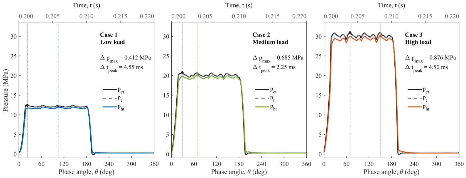
Figure 6 compares the typical-cycle histories of the piston chamber pressure $p_{\mathrm{ct}}$, transition chamber pressure $p_{\mathrm{tr}}$, and central pocket pressure $p_{\mathrm{ht}}$ under low-, medium-, and high-load steady conditions. In some figures, the transition chamber pressure is abbreviated as $p_t$, which has the same physical meaning as $p_{\mathrm{tr}}$ defined in Section 2. Overall, all three pressures pass through suction, pressurization, high-pressure plateau, and depressurization stages within the same rotation period. This indicates that the central pocket pressure is established in response to the piston chamber pressure. However, $p_{\mathrm{ht}}$ is not a lossless copy of $p_{\mathrm{ct}}$. During pressurization and depressurization, the central pocket pressure curve is smoother; in the high-pressure plateau region, the peak value of $p_{\mathrm{ht}}$ is lower than that of $p_{\mathrm{ct}}$, and the peak phases differ. This shows that orifice throttling, chamber compressibility, and sealing-land leakage jointly form a hydraulic transmission unit with buffering characteristics.

Table 2. Steady pressure-transmission statistics.

Case	Load	${\mathit{p}}_{\mathbf{ct},\mathbf{max}}$ (MPa)	${\mathit{p}}_{\mathbf{ht},\mathbf{max}}$ (MPa)	$\mathit{\Delta }{\mathit{p}}_{max}$ (MPa)	${\mathit{\eta }}_{\mathbf{att}}$ (%)	$\mathit{\Delta }{\mathit{t}}_{\mathbf{peak}}$ (ms)	${\mathit{\eta }}_{\mathbf{rate}}$ (%)	${\mathit{p}}_{\mathbf{tr},\mathbf{mean}}$ (MPa)	${\mathit{p}}_{\mathbf{ht},\mathbf{mean}}$ (MPa)
Case 1	Low load	12.4010	11.9885	0.4124	3.33	4.55	7.39	6.1385	5.9621
Case 2	Medium load	20.7702	20.0853	0.6849	3.30	2.25	6.77	10.1719	9.8893
Case 3	High load	30.9598	30.0839	0.8759	2.83	4.50	6.47	15.1192	14.7221

Note: ${\eta }_{\mathrm{att}}$ denotes the peak-pressure attenuation ratio, $\Delta t_{\mathrm{peak}}$ denotes the peak-time difference between $p_{\mathrm{ct}}$ and $p_{\mathrm{ht}}$, and ${\eta }_{\mathrm{rate}}$ denotes the weakening ratio of the maximum pressure-change rate.

gives the statistical results for the three steady cases within the unified cycle window. The piston chamber pressure peaks in Cases 1, 2, and 3 are $12.4010\mathrm{MPa}$, $20.7702\mathrm{MPa}$, and $30.9598\mathrm{MPa}$, respectively. The corresponding central pocket pressure peaks are $11.9885\mathrm{MPa}$, $20.0853\mathrm{MPa}$, and $30.0839\mathrm{MPa}$. The resulting peak attenuation values are $0.4124\mathrm{MPa}$, $0.6849\mathrm{MPa}$, and $0.8759\mathrm{MPa}$ with peak attenuation ratios of $3.33\%$, $3.30\%$, and $2.83\%$, respectively. These results show that under steady periodic pressure input, the central pocket pressure peak is always lower than the piston chamber pressure peak. The peak attenuation does not increase monotonically with load level but rather is jointly affected by the periodic pressure waveform and the two-stage throttling response.

Within the pressurized portions of the steady comparison window, the mean pressures follow $p_{\mathrm{ct}}>p_{\mathrm{tr}}>p_{\mathrm{ht}}>p_{\mathrm{out}}$. A seven-case audit of the formal-grid results showed that the case-wise minimum $p_{\mathrm{ht}}$ remained between $0.1286$ and $0.2724\mathrm{MPa}$ gauge and never reached $p_{\mathrm{out}}$ in the 0.20–0.22 s windows, whereas $p_{\mathrm{tr}}$ reached the numerical floor in 23 of 2800 samples during low-pressure intervals. The hierarchy is therefore interpreted as a pressurized-state/mean-pressure relation rather than a universal inequality during suction and depressurization, and the floor-projected samples are not treated as cavitation predictions.

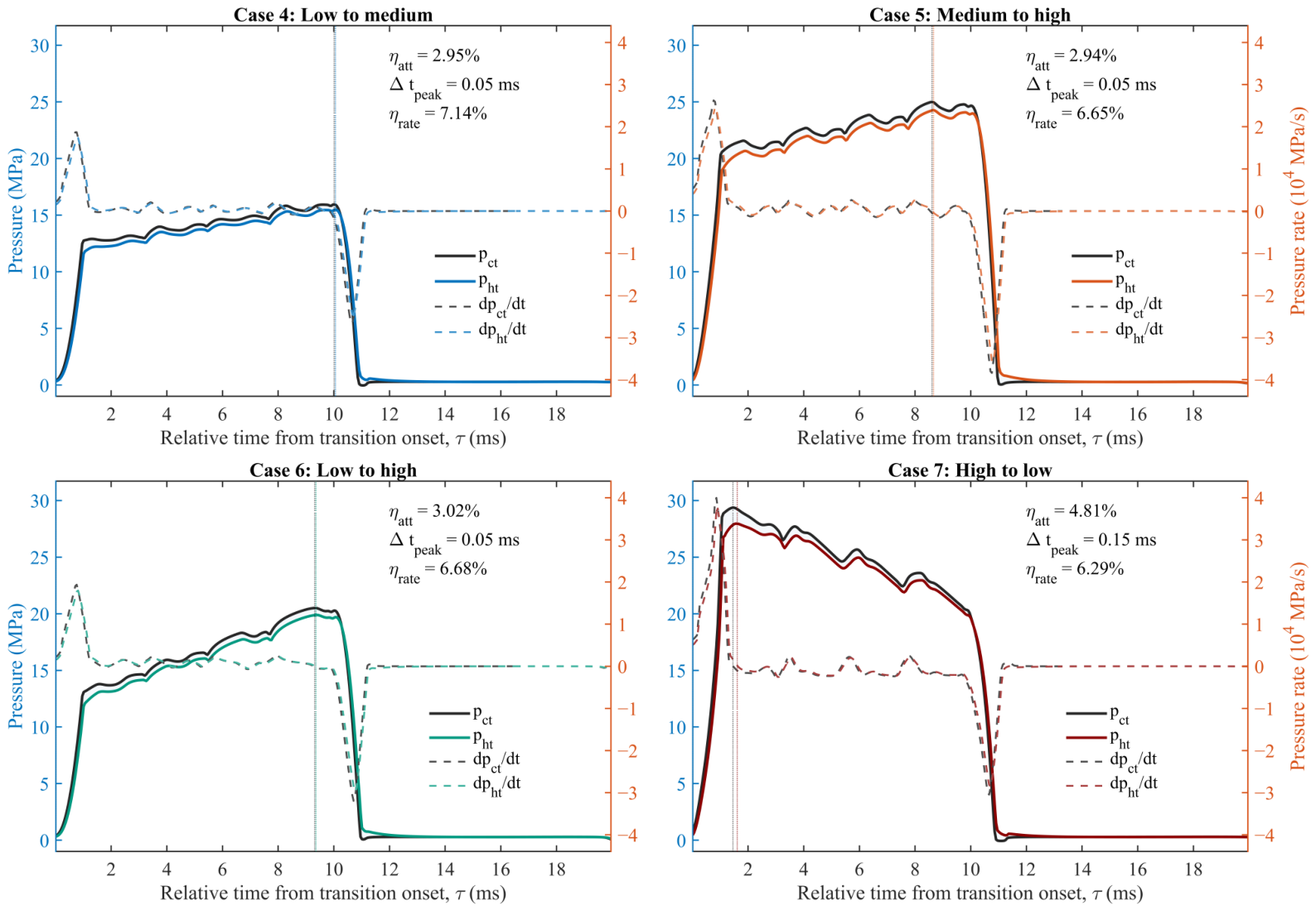
After clarifying the steady pressure transmission characteristics, Figure 7 further presents the local pressure responses of the four variable-load cases during one complete single-cycle load-transition process. Unlike a conventional local segment immediately after a single step input, the variable-load cases in this paper complete one full rotation and the corresponding load-level change within 0.20–0.22 s. Therefore, this window simultaneously includes suction, discharge, load variation, and pressure release phases. Cases 4, 5, 6, and 7 correspond to low-to-medium, medium-to-high, low-to-high, and high-to-low paths, respectively. Figure 7 shows that even under single-cycle load variation, $p_{\mathrm{ht}}$ follows the main pressure pattern of $p_{\mathrm{ct}}$, but its peak amplitude and pressure-rate characteristics remain modulated by the dual-orifice and dual-chamber system.

Table 3. Transient pressure-transmission statistics.

Case	Transition	${\mathit{p}}_{\mathbf{ct},\mathbf{max}}$ (MPa)	${\mathit{p}}_{\mathbf{ht},\mathbf{max}}$ (MPa)	$\mathit{\Delta }{\mathit{p}}_{max}$ (MPa)	${\mathit{\eta }}_{\mathbf{att}}$ (%)	$\mathit{\Delta }{\mathit{t}}_{\mathbf{peak}}$ (ms)	${\mathit{R}}_{\mathbf{ct}}$ (MPa/s)	${\mathit{R}}_{\mathbf{ht}}$ (MPa/s)	${\mathit{\eta }}_{\mathbf{rate}}$ (%)
Case 4	Low–medium	15.9590	15.4885	0.4706	2.95	0.05	26639.30	24735.96	7.14
Case 5	Medium–high	25.0022	24.2664	0.7358	2.94	0.05	38431.86	35877.54	6.65
Case 6	Low–high	20.5098	19.8913	0.6185	3.02	0.05	31960.38	29824.46	6.68
Case 7	High–low	29.3719	27.9595	1.4124	4.81	0.15	39971.25	37458.92	6.29

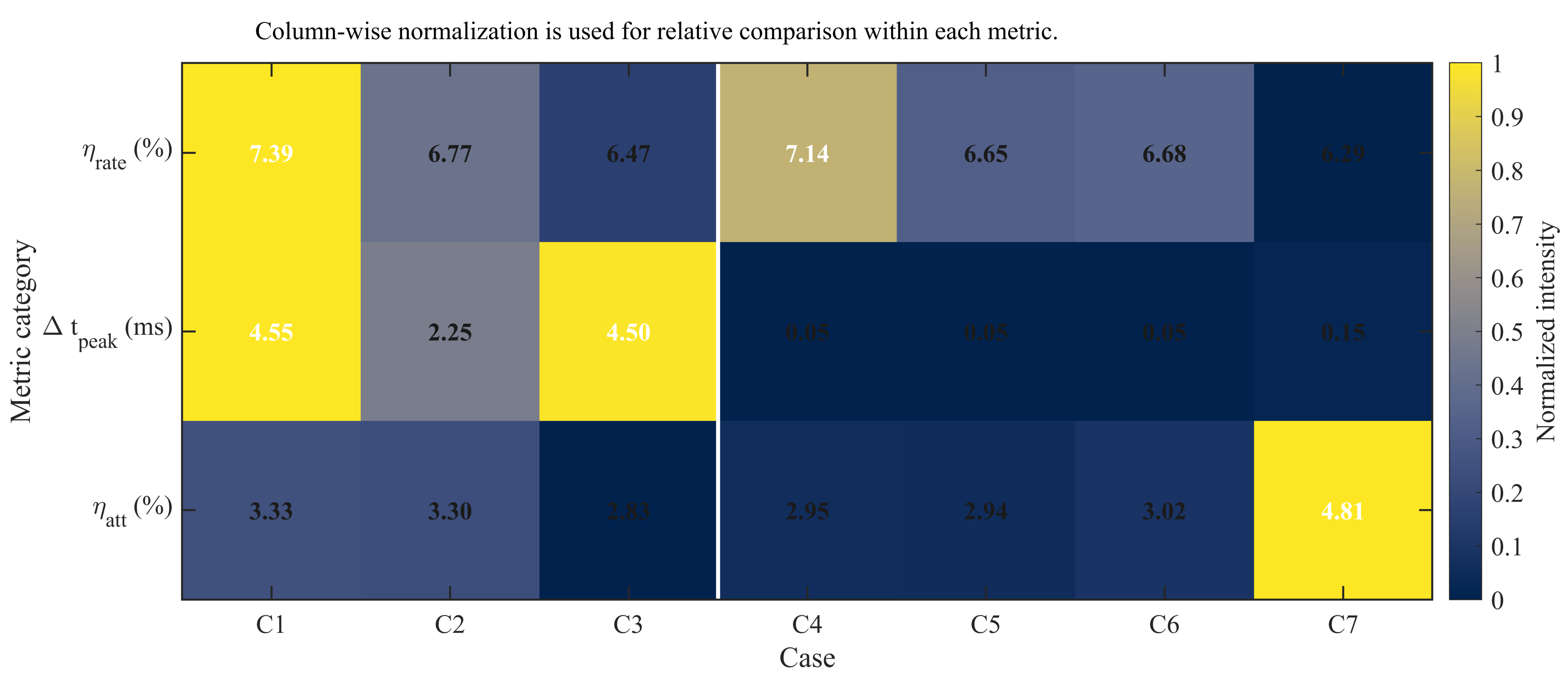
Note: $R_{\mathrm{ct}}=max|\mathrm{d}{p}_{ct}/\mathrm{d}t|$  and  $R_{\mathrm{ht}}=max\left|\mathrm{d}{p}_{\mathrm{ht}}/\mathrm{d}t\right|$ denote the maximum pressure-change rates in the piston chamber and central pocket, respectively.

shows that the peak attenuation ratios of Cases 4, 5, 6, and 7 are $2.95\%$, $2.94\%$, $3.02\%$, and $4.81\%$, respectively. The corresponding peak-time differences are $0.05\mathrm{ms}$, $0.05\mathrm{ms}$, $0.05\mathrm{ms}$, and $0.15\mathrm{ms}$. Compared with steady periodic waveforms, the global pressure peak in variable-load cases is usually controlled by the main pressure peak or residual high-pressure region within the same full rotation period. Thus, the peak-time difference between $p_{\mathrm{ct}}$ and $p_{\mathrm{ht}}$ is significantly reduced. The values of $\Delta t_{\mathrm{peak}}$ are close to the sampling resolution of the time-history data and therefore should not be interpreted alone as the main evidence for the buffering capacity under variable loading.

It should be noted that Case 6 represents a large-amplitude loading command from low to high load, but this does not mean that the highest pressure level is reached at every phase within the selected single cycle. Because the load-establishment process is superposed with the porting phase, the actual piston chamber pressure peak of Case 6 in the current cycle is lower than that of Case 5. This indicates that the variable-load pressure response is jointly controlled by the load amplitude and cycle phase. This observation is also consistent with CFD studies showing that instantaneous clearance and pressure distribution in slipper pairs are jointly modulated by the relative posture and porting phase [17,28].

Compared with the peak-time difference, the pressure-rate weakening provides a more stable indicator for the variable-load cases. Table 3 shows that the ${\eta }_{\mathrm{rate}}$ values of Cases 4–7 are $7.14\%$, $6.65\%$, $6.68\%$, and $6.29\%$, respectively. In other words, even when the peak times of $p_{\mathrm{ct}}$ and $p_{\mathrm{ht}}$ are nearly synchronized, the maximum pressurization or depressurization rate of the central pocket pressure remains clearly lower than that of the piston chamber pressure. This result indicates that during the complete single-cycle variable-load process, the main buffering effect of the dual-orifice and dual-chamber structure is not necessarily expressed as a large shift in peak time but rather more directly as pressure-rate weakening and pressure-curve smoothing.

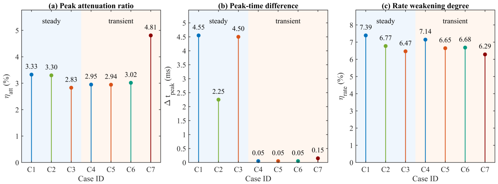
Figure 8 compares ${\eta }_{\mathrm{att}}$, $\mathsf{\Delta }{t}_{\mathrm{peak}}$, and ${\eta }_{\mathrm{rate}}$ across all cases. The high value of the peak attenuation ratio is concentrated in Case 7, indicating that the pressure-amplitude buffering is strongest under the high-to-low unloading path. High values of the peak-time difference mainly appear in steady Cases 1 and 3, reflecting a more pronounced phase shift of the central pocket pressure peak relative to the piston chamber pressure peak in steady periodic waveforms. The pressure-rate weakening is relatively high in Cases 1 and 4, indicating that low-load steady and low-to-medium variable-load processes are more sensitive to pressure-rate modulation. A column-normalized heatmap of the same three indicators is provided in Figure A1 to show the relative strength distribution within each metric column. Its color intensity is used only for within-metric comparison and should not be interpreted as an absolute comparison among different indicators.

Combining Figure 6, Figure 7 and Figure 8 and Table 2 and Table 3, the dual-orifice and dual-chamber system transforms the piston chamber pressure into a smoother and physically bounded central pocket pressure through orifice pressure drop, chamber compressibility, and sealing-land leakage. This transformation is expressed as peak attenuation, peak-time difference, and pressure-rate weakening. For steady periodic pressure input, the peak phase shift reflects the periodic response difference between the central pocket pressure and piston chamber pressure. For the single-cycle variable-load process, the pressure-rate weakening better characterizes the smoothing effect of the pressure transmission chain on the transient input. Therefore, $p_{\mathrm{ht}}$ is used as the unified local pressure boundary for the subsequent slipper posture, three-dimensional flow–thermal, and structural-response analyses rather than directly imposing $p_{\mathrm{ct}}$ at the local slipper-pair inlet.

3.2. Evolution of Slipper Micro-Motion Posture Under Transient Pressure Excitation

Based on the corrected central-pocket pressure boundary obtained in Section 3.1, this section analyzes how $p_{\mathrm{ht}}\left(t\right)$ is transformed into slipper micro-motion and the instantaneous clearance field. The time-history evolution of the central film thickness $h_0$, minimum film thickness $h_{min}$, and tilt components ${\alpha }_x$ and ${\alpha }_y$ is examined to clarify the kinematic response of the slipper bottom. The coupling between slipper posture and oil-film thickness has been discussed in lubrication and vibration–lubrication studies, indicating that the central film thickness and tilt variables are important indicators of slipper micro-motion [7,8].

Section 2 has defined the posture variables, instantaneous clearance reconstruction relation, and local lubrication solution method. These formulae are not repeated here. To compare posture variations among different cases, the tilt magnitude $\left|\alpha \right|={({\alpha }_x^2+{\alpha }_y^2)}^{1/2}$ and the film-thickness uniformity index ${\eta }_p=h_{min}/h_0$ are also used. Here, $\left|\alpha \right|$ represents the overall tilting level, while ${\eta }_p$ describes the retention of the local minimum film thickness relative to the central film thickness. It should be noted that ${\eta }_p$ is only a descriptive indicator of posture uniformity. An increase in ${\eta }_p$ indicates a more uniform bottom clearance distribution, but it does not imply a strictly parallel support state.

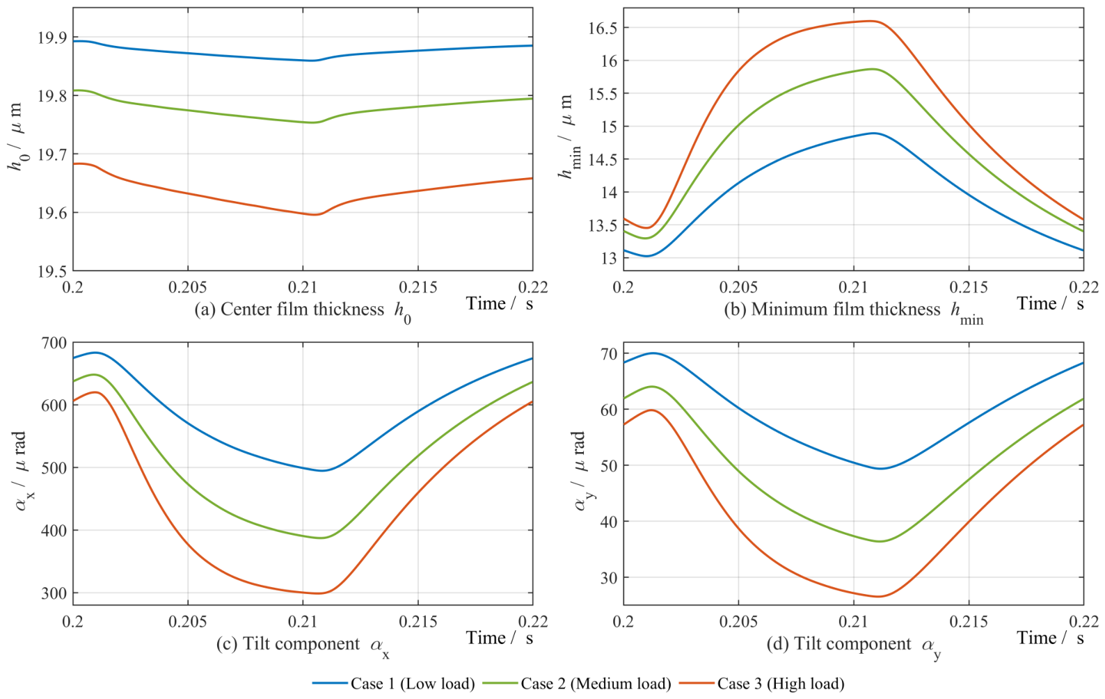
Figure 9 shows the time histories of slipper posture variables over a complete cycle under the three steady load levels. The variables $h_0$, $h_{min}$, ${\alpha }_x$, and ${\alpha }_y$ all exhibit periodic fluctuations, but their sensitivities to load variation differ. The central film thickness $h_0$ mainly reflects the overall axial floating or sinking of the slipper, and its variation amplitude is relatively small. The minimum film thickness $h_{min}$ is affected by both the overall film thickness and the tilting posture, and it is more sensitive to the geometric constraint of local thin-film regions. In the coordinate definition used in this paper, the magnitude of ${\alpha }_x$ is much larger than that of ${\alpha }_y$, indicating that the slipper posture variation within the present case window is dominated by the x-direction tilt component, while the y-direction component is relatively weak.

Table 4. Steady posture statistics at the minimum-film-thickness instant.

Case	Load	${\mathit{t}}_{\mathit{d}}$ (ms)	${\mathit{h}}_{min}$ ($\mathsf{\mu }$m)	$\left|\mathit{\alpha }\right|$ ($\mathsf{\mu }$rad)	${\mathit{\eta }}_{\mathit{p}}$
1	Low	1.01	13.024	686.67	0.6548
2	Medium	0.96	13.293	651.10	0.6712
3	High	1.01	13.452	622.68	0.6836

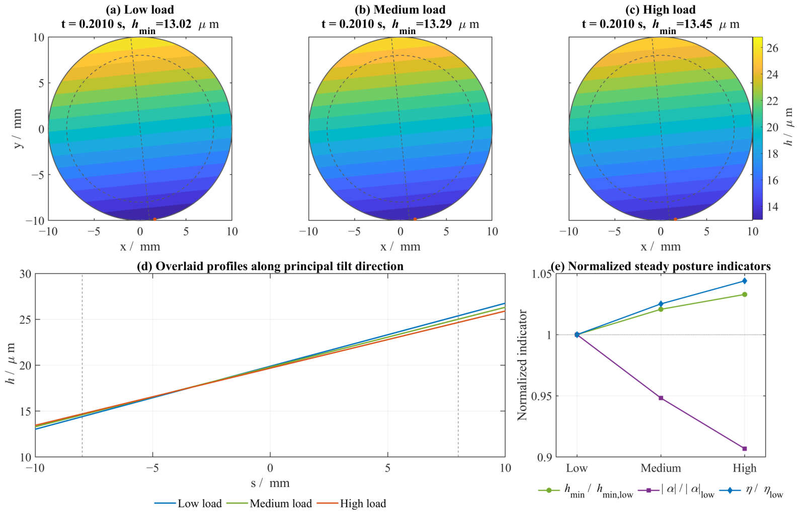
Note: t_d is the time at which h_min reaches its minimum within the observation window of each steady case.

lists the posture statistics at the minimum-film-thickness instant for the three steady cases. In this paper, $t_d$ denotes the time at which $h_{min}$ reaches its minimum within the observation window of each steady case; this instant is defined as the steady critical instant, and $h_{min}$, $\left|\alpha \right|$, and ${\eta }_p$ are evaluated at $t_d$. As the load increases from low to high, $h_{min}$ increases from $13.024\mathsf{\mu }\mathrm{m}$ to $13.452\mathsf{\mu }\mathrm{m}$, $\left|\alpha \right|$ decreases from $686.67\mathsf{\mu }\mathrm{rad}$ to $622.68\mathsf{\mu }\mathrm{rad}$, and ${\eta }_p$ increases from $0.6548$ to $0.6836$. These results indicate that within the steady load range considered in this paper, increasing load does not further reduce the local minimum film thickness. Instead, the smaller tilt magnitude makes the bottom clearance distribution more uniform, causing the minimum film thickness to increase.

Figure 10 further presents the spatial reconstruction of film thickness at the key instants for the three steady load levels. The upper-row film-thickness maps show that the low-load case has a more obvious tilting gradient and a more concentrated minimum-film-thickness region. As the load increases, the film-thickness distribution becomes more uniform and the film-thickness difference along the principal tilt direction decreases. The lower-row overlapped profiles and normalized indicator plot further indicate that although the high-load case is accompanied by a slight reduction in central film thickness, it has a smaller tilt magnitude and a higher film-thickness uniformity index. Thus, the influence of increasing steady load on slipper posture is not simply reflected as overall sinking but also as reduced tilting and improved clearance uniformity. Within the current parameter range, the beneficial effect of tilt reduction on the minimum film thickness exceeds the possible adverse effect of reduced central film thickness.

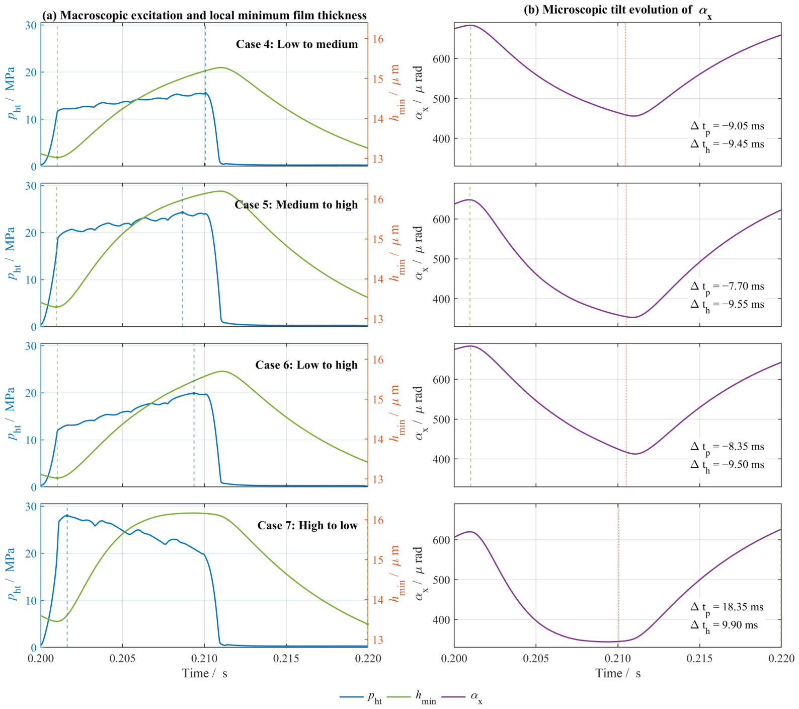
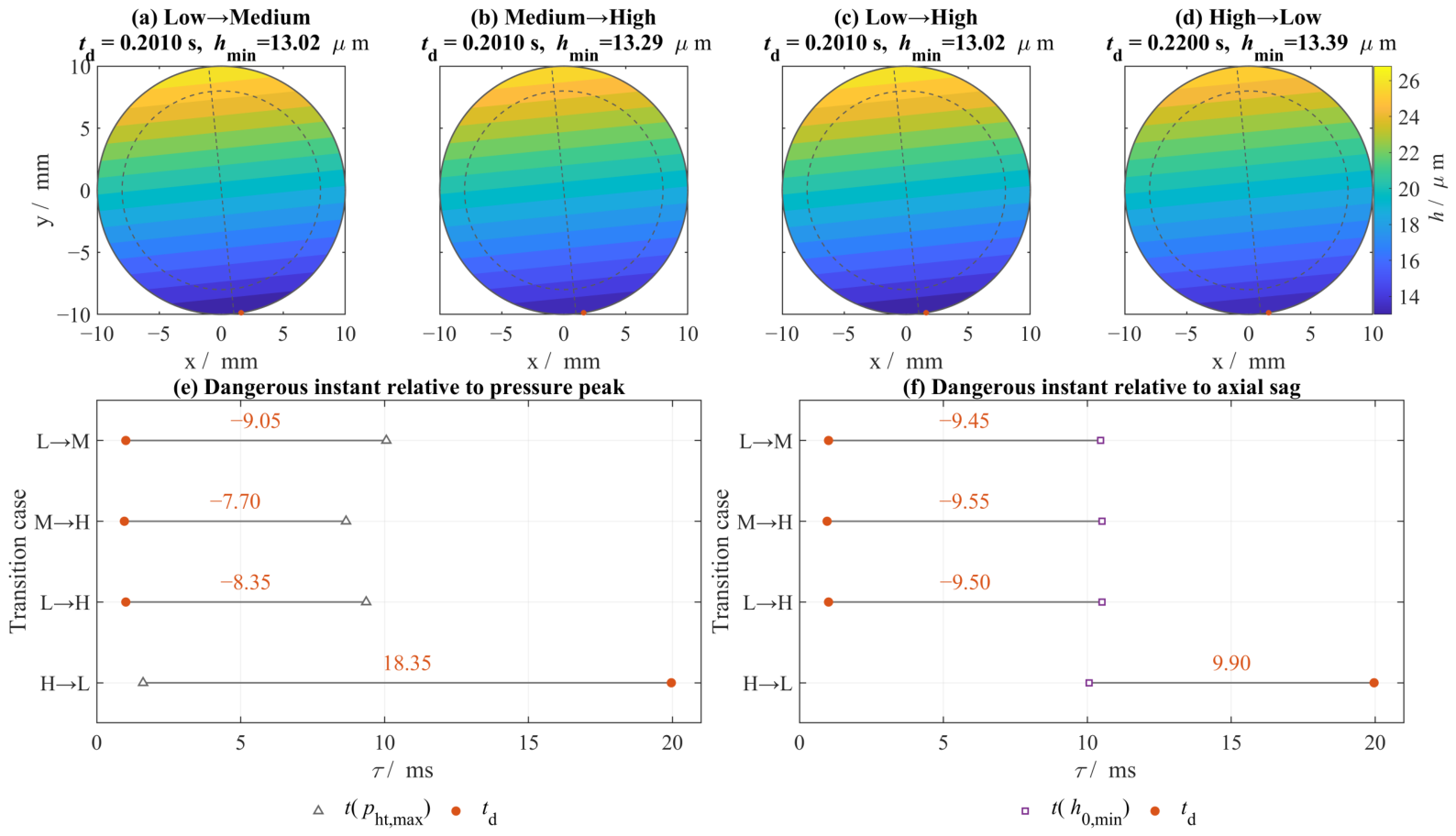
For the variable-load cases, the full-cycle window defined in Section 2 is used for analysis. This window is not a local segment before and after a single transition but rather a complete transition cycle that includes discharge, suction, and load-level variation within one rotation period. Therefore, the posture response under variable loading should not be simplified into a two-stage comparison of “before” and “after” a transition. Instead, the phase relationships among pressure peak, overall sinking, and minimum film thickness should be analyzed over the complete cycle. To describe this phase relationship, the time at which $h_{min}$ reaches its minimum within the window is denoted by $t_d$, while the central pocket pressure peak time and central film-thickness minimum time are denoted by $t_p=t\left(p_{\mathrm{ht},\max }\right)$ and $t_h=t\left(h_{0,min}\right)$, respectively. The time differences are defined as $\mathsf{\Delta }{t}_p=t_d-t_p$ and $\mathsf{\Delta }{t}_h=t_d-t_h$. Here, $\mathsf{\Delta }{t}_p<0$ means that the minimum film thickness occurs before the central pocket pressure peak, while $\mathsf{\Delta }{t}_h<0$ means that the minimum film thickness occurs before the maximum overall sinking.

Figure 11 shows the local time-history responses of the four variable-load cases over the complete transition cycle. Compared with the steady cases, the phase relationship among $p_{\mathrm{ht}}$, $h_{min}$, and ${\alpha }_x$ becomes more complex. The central pocket pressure peak does not necessarily coincide with the minimum film thickness, and the minimum central film thickness does not necessarily correspond to the minimum film thickness. This indicates that over the complete transition cycle, the formation of the minimum film thickness depends not only on the pressure peak magnitude but also on the porting phase at which the peak occurs and the historical state of slipper tilting at that time. CFD studies with continuously updated slipper positions also show that slipper translation and tilting can change the instantaneous clearance and flow-field response [17,28]. In other words, the minimum film-thickness state results from the coupled effects of pressure input, overall axial displacement, and tilting posture.

Table 5. Transient posture and phase-timing statistics at the minimum-film-thickness instant.

Case	Path	${\mathit{t}}_{\mathit{p}}$ (ms)	${\mathit{t}}_{\mathit{h}}$ (ms)	${\mathit{t}}_{\mathit{d}}$ (ms)	${\mathit{h}}_{min}$ ($\mathsf{\mu }$m)	$\left|\mathit{\alpha }\right|$ ($\mathsf{\mu }$rad)	${\mathit{\eta }}_{\mathit{p}}$	$\mathit{\Delta }{\mathit{t}}_{\mathit{p}}$ (ms)	$\mathit{\Delta }{\mathit{t}}_{\mathit{h}}$ (ms)
4	L→M	10.06	10.46	1.01	13.024	686.68	0.6548	−9.05	−9.45
5	M→H	8.66	10.51	0.96	13.293	651.13	0.6712	−7.70	−9.55
6	L→H	9.36	10.51	1.01	13.023	686.69	0.6548	−8.35	−9.50
7	H→L	1.61	10.06	19.96	13.386	628.92	0.6804	18.35	9.90

Note: The times $t_p$, $t_h$, and $t_d$ denote the central-pocket pressure peak time, central film-thickness minimum time, and local minimum-film-thickness time within the local cycle, respectively.

gives the posture and phase-timing statistics at the minimum-film-thickness instant for the four variable-load cases. For Cases 4 (low to medium), 5 (medium to high), and 6 (low to high), $t_d$ is located in the early stage of the cycle at approximately $1.01\mathrm{ms}$, $0.96\mathrm{ms}$, and $1.01\mathrm{ms}$, respectively. The corresponding $t_p$ values are approximately $10.06\mathrm{ms}$, $8.66\mathrm{ms}$, and $9.36\mathrm{ms}$. Therefore, $\mathsf{\Delta }{t}_p$ is negative for all three loading cases with values of $-9.05\mathrm{ms}$, $-7.70\mathrm{ms}$, and $-8.35\mathrm{ms}$. The values of $\mathsf{\Delta }{t}_h$ are also negative—namely, $-9.45\mathrm{ms}$, $-9.55\mathrm{ms}$, and $-9.50\mathrm{ms}$. This indicates that during the loading transition cycle, the minimum film thickness is not directly triggered during the central pocket pressure peak stage but rather appears earlier near the initial phase of the cycle.

In contrast to the loading cases, Case 7 (high to low) exhibits an opposite phase characteristic. Its central pocket pressure peak is located in the early stage of the cycle, with $t_p\approx 1.61\mathrm{ms}$, while the window minimum-film-thickness instant $t_d$ appears near the end of the cycle at approximately $19.96\mathrm{ms}$, corresponding to $\mathsf{\Delta }{t}_p=18.35\mathrm{ms}$. Meanwhile, $\mathsf{\Delta }{t}_h=9.90\mathrm{ms}$, indicating that the minimum film thickness also lags behind the minimum central film thickness. This result suggests that during the high-to-low unloading process, pressure release does not immediately improve the local clearance. The recovery of slipper posture lags behind pressure release, and the local film-thinning risk is more strongly controlled by posture adjustment in the later part of the cycle.

The upper row of Figure 12 further verifies the above observations through film-thickness reconstruction. At the window minimum-film-thickness instants, all four variable-load cases exhibit non-uniform film-thickness distributions, but their phase locations and posture origins differ. In Cases 4, 5, and 6, the minimum-film-thickness state mainly reflects the continuation of the early-cycle posture state, whereas in Case 7, it appears near the end of the cycle and reflects delayed posture adjustment during unloading. The lower-row timing comparison in Figure 12 directly compares $t_p$, $t_h$, and $t_d$, further indicating that the minimum film thickness, pressure peak, and overall sinking are not synchronized. Therefore, the film-thinning risk under variable loading cannot be judged only from the pressure peak or central film-thickness extremum but rather must be identified by considering the two-dimensional tilting posture and full-cycle phase.

Taken together, Figure 9, Figure 10, Figure 11 and Figure 12 and Table 4 and Table 5 indicate two main features of slipper micro-motion posture response. First, within the steady load range, increasing load makes the slipper posture more uniform, which is reflected by a reduced tilt magnitude, increased film-thickness uniformity index, and increased minimum film thickness. Second, within the complete variable-load cycle, the minimum film thickness is clearly asynchronous with the central pocket pressure peak and the central film-thickness minimum. In loading cases, the window minimum film thickness tends to occur in the early cycle and is more closely controlled by the inherited initial posture. In the unloading case, the window minimum film thickness shifts toward the end of the cycle and reflects delayed posture recovery. Therefore, slipper posture acts as a temporal–spatial filter between the scalar pressure boundary and the downstream three-dimensional flow field: it converts $p_{\mathrm{ht}}\left(t\right)$ into a history-dependent clearance distribution $h(x,y,t)$ through overall floating, tilting adjustment, and posture inheritance.

These results provide the direct geometric basis for the subsequent three-dimensional flow–thermal calculation. Because the instantaneous slipper-bottom clearance evolves with $h_0$, ${\alpha }_x$, and ${\alpha }_y$, a fixed parallel clearance in the three-dimensional model would fail to represent the spatial redistribution of local thin-film regions caused by posture evolution. Therefore, Section 3.3 uses the key-instant posture and film-thickness reconstruction results identified in this section as geometric inputs to further analyze the pressure and temperature-rise fields under transient posture conditions.

3.3. Transient Pressure–Temperature Field Evolution Under Posture-Dependent Clearance

Section 3.1 shows that the central pocket pressure $p_{\mathrm{ht}}$, rather than the piston chamber pressure $p_{\mathrm{ct}}$, is the actual inlet pressure boundary for the three-dimensional flow–thermal calculation after modulation by the dual-orifice and dual-chamber system. Section 3.2 further shows that the central pocket pressure is not converted into a synchronous film-thickness response but rather reconstructs the instantaneous slipper-bottom clearance through the combined variations of the central film thickness $h_0$ and the tilt components ${\alpha }_x$ and ${\alpha }_y$. Based on the pressure boundary and posture boundary established in the previous sections, this section analyzes the transient evolution of the three-dimensional oil-film pressure field and temperature-rise field of the slipper pair under different load levels and variable-load paths.

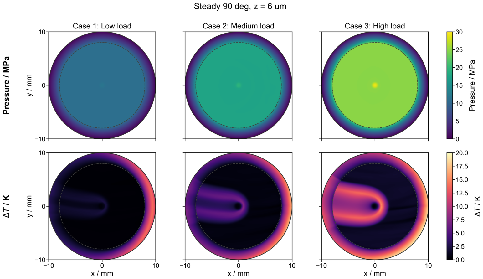
The pressure boundary import, posture moving boundary, mesh update, and thermal boundary settings in Fluent have been described in Section 2. Therefore, this section does not repeat the governing equations or numerical implementation details. Instead, it focuses on two questions: first, how the pressure field and temperature-rise field spatially expand as the steady load increases; second, whether the temperature-rise peak under variable loading remains synchronized with the instantaneous pressure peak or target load level. To combine spatial distribution and cyclic thermal response, two types of evidence are used. First, pressure and temperature-rise contours are extracted from the $z=6\mathsf{\mu }\mathrm{m}$ oil-film section to compare the bearing region and local thermal concentration among cases. Second, the maximum temperature rise in the full fluid domain is extracted to characterize single-cycle heat accumulation and phase lag. The $z=6\mathsf{\mu }\mathrm{m}$ section is selected because it avoids any over-amplification of near-wall local boundary effects while clearly presenting spatial differences in oil-film temperature rise.

Figure 13 shows the pressure and temperature-rise distributions for steady Cases 1–3 at the ${90}^{\circ }$ phase, corresponding to the middle stage of the discharge process. As the load increases from low to high, the maximum sectional pressure increases from $11.68\mathrm{MPa}$ to $19.43\mathrm{MPa}$ and $29.23\mathrm{MPa}$, while the area-averaged pressure increases from $9.16\mathrm{MPa}$ to $14.39\mathrm{MPa}$ and $20.14\mathrm{MPa}$. This indicates that increasing the steady load not only raises the local pressure peak but also increases the average load-carrying level over the entire oil-film region. Correspondingly, the maximum sectional temperature rise increases from $13.75\mathrm{K}$ to $16.92\mathrm{K}$ and $19.24\mathrm{K}$, while the area-averaged temperature rise increases from $1.84\mathrm{K}$ to $3.07\mathrm{K}$ and $5.72\mathrm{K}$. Thus, during the middle discharge phase, the enhanced thermal response under high steady load is not expressed only as an increase in a single hot spot but rather as the combined result of an expanded high-pressure bearing region and an expanded temperature-rise region.

The spatial distributions complement the posture response discussed in Section 3.2. Section 3.2 shows that within the steady load range considered here, increasing load reduces the slipper tilt magnitude, increases the film-thickness uniformity index, and prevents the local minimum film thickness from deteriorating synchronously with the decrease in central film thickness. Figure 13 further shows that even when the slipper-bottom clearance distribution becomes more uniform, the higher central pocket pressure and stronger oil-film shear under high load still significantly increase the fluid-domain temperature rise. The influence of posture updating on pressure distribution, leakage, and local flow state has been verified in slipper-pair CFD studies [17,28]. Therefore, the steady flow–thermal response should not be attributed simply to changes in the local minimum film thickness but rather should be understood as the combined effect of the central pocket pressure boundary, instantaneous clearance distribution, and viscous shear dissipation.

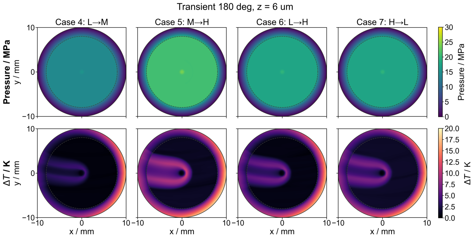
Figure 14 presents the pressure and temperature-rise fields for variable-load Cases 4–7 at the ${180}^{\circ }$ phase, corresponding to the end of the discharge stage or the beginning of the suction stage. For the three loading cases, Cases 4 (low to medium), 5 (medium to high), and 6 (low to high), the maximum sectional pressures are $15.47\mathrm{MPa}$, $23.96\mathrm{MPa}$, and $19.66\mathrm{MPa}$, respectively, and the corresponding maximum sectional temperature rises are $16.98\mathrm{K}$, $18.45\mathrm{K}$, and $17.25\mathrm{K}$. The pressure peak and temperature-rise peak of Case 5 are both higher than those of Case 6. Case 6 represents a large-amplitude low-to-high load command, but this does not mean that the highest pressure is reached at every phase within the selected single cycle. Because the load-establishment process is superposed with the porting phase, the actual pressure peak of Case 6 at the current phase is lower than that of Case 5, indicating that the variable-load flow–thermal response is jointly controlled by the load amplitude and cycle phase.

For Case 7 (high to low), although the target load has switched from high to low, the maximum sectional pressure at the ${180}^{\circ }$ phase remains $19.60\mathrm{MPa}$, which is close to that of Case 6. Its maximum sectional temperature rise is $17.95\mathrm{K}$, which is higher than that of Case 6. This result indicates that during high-to-low unloading, the oil-film flow–thermal field does not immediately recover to the low-load state after the target load is reduced. Instead, it retains the influence of the pressure and heat accumulation from the preceding high-load stage for a certain period. The influence of thermal effects on the load-carrying capacity and temperature rise of slipper pairs has been discussed in thermoelastohydrodynamic and thermal–mechanical coupling studies [18,21,22]. Considering the modulated pressure release in Case 7 shown in Section 3.1 and the delayed minimum film thickness near the end of the cycle shown in Section 3.2, the unloading case exhibits a clear phase mismatch among pressure decay, posture recovery, and thermal response.

To avoid the limitation of judging thermal response from a single section or a single phase, the maximum temperature rise in the full fluid domain is introduced as a cyclic thermal-load indicator:    

$$\mathsf{\Delta }{T}_{max,\mathsf{\Omega }}\left(t\right)=T_{max}\left(t\right)-T_{\mathrm{in}}.$$

(19)

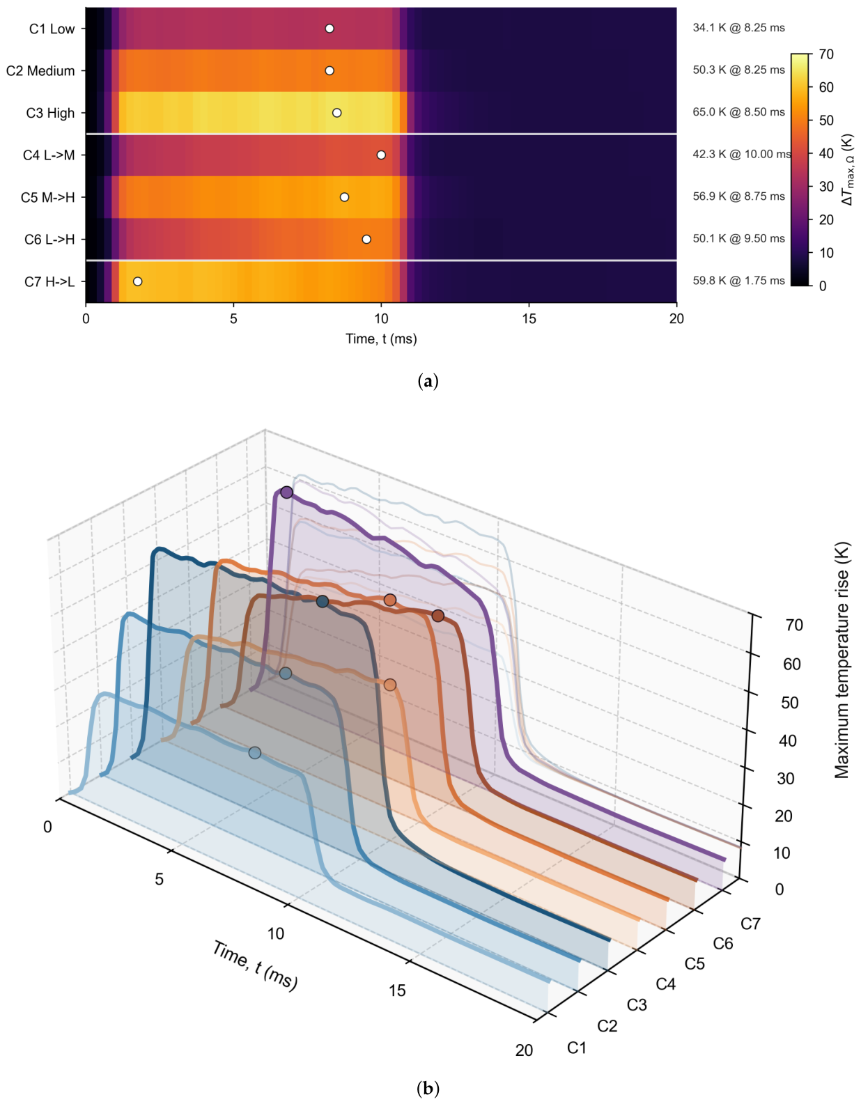
Here, $T_{max}\left(t\right)$ is the maximum temperature in the Fluent fluid domain at the current time, and $T_{\mathrm{in}}$ is the inlet temperature. For consistency, all absolute maximum temperatures reported in the Results section are expressed in °C, whereas temperature rises $\mathsf{\Delta }T$ are expressed in K. Fluent continues to use absolute temperature in K internally; the reported absolute values are converted using $T{(}^{\circ }\mathrm{C})=T\left(\mathrm{K}\right)-273.15$. Figure 15a shows the heatmap of the full-domain maximum temperature rise for the seven cases over one cycle, while Figure 15b presents the corresponding temperature-rise histories in a waterfall format. The temperature rise does not reach its peak instantaneously with changes in the pressure boundary. Instead, each case undergoes rapid heating, peak retention, or slow decay within the cycle. This indicates that the oil-film temperature field has thermal inertia relative to pressure input and posture variation. The localized temperature rise depends not only on the current pressure level but also on the preceding high-pressure stage, local shear dissipation, and heat transport within the oil film. Similar thermal inertia and thermal–mechanical coupling effects are central issues in TEHD models and thermoelastic multibody models [19,21].

Table 6. Full-domain temperature-rise peak statistics across seven load cases.

Case	Condition	Path	${\mathit{t}}_{\mathbf{peak}}$ (ms)	$\mathit{\Delta }{\mathit{T}}_{max}$ (K)	${\mathit{T}}_{max}$ (°C)
1	Case 1	Low steady	8.25	34.12	60.97
2	Case 2	Medium steady	8.25	50.25	77.10
3	Case 3	High steady	8.50	65.01	91.86
4	Case 4	Low to medium	10.00	42.33	69.18
5	Case 5	Medium to high	8.75	56.89	83.74
6	Case 6	Low to high	9.50	50.13	76.98
7	Case 7	High to low	1.75	59.76	86.61

summarizes the full-domain temperature-rise peaks for the seven cases. Under steady loading, the maximum temperature rises of Cases 1, 2, and 3 are $34.12\mathrm{K}$, $50.25\mathrm{K}$, and $65.01\mathrm{K}$, respectively, corresponding to maximum temperatures of 60.97 °C, 77.10 °C, and 91.86 °C. The temperature-rise peaks of all three cases occur in the first half of the cycle. The low- and medium-load peaks both occur at $8.25\mathrm{ms}$, while the high-load peak occurs at $8.50\mathrm{ms}$. This indicates that under steady periodic response, increasing load significantly increases the thermal load of the oil-film region, while the phase of the maximum temperature rise remains relatively concentrated among the steady load levels.

The reported absolute oil-film temperatures are conditional on the zero-heat-flux fluid-side wall boundary. Applying the same boundary treatment to all seven cases supports their comparison within the present model, but the reported values should not be interpreted as conjugate fluid–solid interface temperatures.

Under variable loading, the temperature-rise peak is no longer determined solely by the target load level or load-change amplitude, but it exhibits stronger path dependence. The maximum temperature rises of Cases 4, 5, 6, and 7 are $42.33\mathrm{K}$, $56.89\mathrm{K}$, $50.13\mathrm{K}$, and $59.76\mathrm{K}$, respectively. The peak times of the loading cases are mainly concentrated near the middle of the cycle: $10.00\mathrm{ms}$, $8.75\mathrm{ms}$, and $9.50\mathrm{ms}$ for Cases 4, 5, and 6, respectively. In contrast, the temperature-rise peak of Case 7 appears at $1.75\mathrm{ms}$, which is much earlier than those of the other variable-load cases. This phenomenon indicates that the thermal peak in the high-to-low unloading process is mainly inherited from the high-load pressure and heat-accumulation state in the early cycle rather than being generated during the later low-load stage.

Overall, Figure 13, Figure 14 and Figure 15 and Table 6 indicate that the three-dimensional pressure–temperature response of the slipper pair is governed by three coupled factors: pressure-driven load carrying, posture-modulated clearance, and thermal-inertia retention. First, the central pocket pressure determines the basic intensity of oil-film load carrying and shear dissipation, and increasing load raises both the pressure level and the thermal load. Second, the slipper posture modifies local flow passages by changing the instantaneous clearance distribution, so the pressure and temperature-rise fields are not determined only by the target load level but also by cycle phase and inherited posture state. Third, the temperature field has thermal inertia relative to pressure input and posture variation, so the maximum temperature rise may not be synchronized with the pressure peak, central film-thickness extremum, or minimum-film-thickness instant.

Therefore, in the subsequent structural response analysis, the thermal-load input should not be selected solely based on a single pressure peak or the minimum-film-thickness instant. Instead, it should consider the full-cycle pressure and temperature-rise histories and the corresponding phase of the fluid-domain thermal peak. The transient pressure and temperature fields obtained in this section provide the load basis for the structural thermal–mechanical response analysis in Section 3.4. The integrated identification of candidate high-risk regions is further completed in Section 3.5 by combining the film-thickness envelope field, oil-film temperature-rise envelope field, and structural stress envelope field.

3.4. Structural Response Under Pressure and Thermal Loads

The flow–thermal results in Section 3.3 show that the pressure field and temperature-rise field in the oil film exhibit clear spatial redistribution and phase differences under posture-dependent clearance conditions. To further determine how these fluid-domain loads are transferred into the slipper body, the transient pressure and temperature fields obtained from the CFD calculation were mapped onto a single-slipper transient structural model. More precisely, the pressure field was transferred directly from Fluent, while two mapped oil-facing surface-temperature histories were first used to solve transient heat conduction in the bronze slipper, and the resulting solid-temperature field was then transferred to the structural analysis. Bronze conduction is therefore included downstream, but the thermally induced components of deformation and stress remain conditioned by the upstream zero-heat-flux Fluent boundary because no solid-to-fluid heat-flux feedback is included. Since the structural model in this paper contains only the slipper body, without the swash plate or a slipper–swash-plate contact pair, this section focuses only on the transient thermal–mechanical response of the slipper structure. The contact pressure, contact state, contact clearance, swash-plate deformation, and two-body contact response are therefore not considered. Following the evidence boundary of this paper, this section identifies structural high-response features within the single-slipper model rather than final failure, wear, or contact-damage regions.

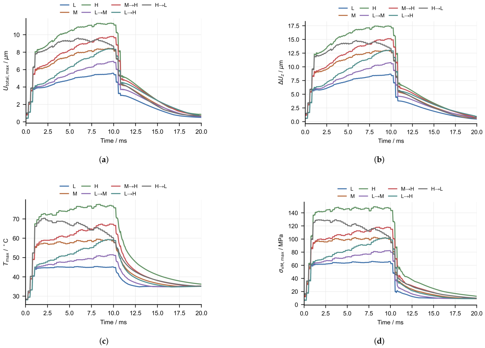
The structural response was evaluated over the same local cycle of 0–$20\mathrm{ms}$. The main-text quantities include the maximum total deformation $U_{\mathrm{total},\max }$, the normal deformation range $U_{z,\mathrm{range}}=U_{z,max}-U_{z,min}$, the maximum von Mises equivalent stress ${\sigma }_{\mathrm{vM},\max }$, the maximum principal stress $S_{1,max}$, the minimum principal stress $S_{3,min}$, and the maximum structural temperature $T_{max}$. The corresponding peak instants $t_U$, $t_{Uz}$, $t_{\sigma }$, and $t_T$ were used to examine whether deformation, normal warpage, stress concentration, and thermal response occur synchronously. The maximum equivalent elastic strain $E_{\mathrm{eqv},\max }$ is retained as an auxiliary structural-response quantity in the full source data, but it is not listed as a main-text column in

Table 7. Structural-response peak statistics across seven load cases.

Case	Condition	${\mathit{U}}_{\mathbf{total},\mathbf{max}}$ ($\mathsf{\mu }$m)	${\mathit{t}}_{\mathit{U}}$ (ms)	${\mathit{U}}_{\mathit{z},\mathbf{range},\mathbf{max}}$ ($\mathsf{\mu }$m)	${\mathit{t}}_{\mathbf{Uz}}$ (ms)	${\mathit{\sigma }}_{\mathbf{vM},\mathbf{max}}$ (MPa)	${\mathit{t}}_{\mathit{\sigma }}$ (ms)	${\mathit{S}}_{1,max}$ (MPa)	${\mathit{S}}_{3,min}$ (MPa)	${\mathit{T}}_{max}$ (°C)	${\mathit{t}}_{\mathit{T}}$ (ms)
Case 1	Low steady	5.59	9.95	8.68	9.95	65.89	7.95	79.35	−103.81	45.35	8.05
Case 2	Medium steady	8.45	9.45	13.04	9.45	102.68	8.20	125.58	−160.39	59.49	8.05
Case 3	High steady	11.34	9.75	17.47	9.75	149.37	8.25	168.07	−217.16	77.52	8.30
Case 4	Low to medium	6.95	9.95	10.77	9.95	82.32	9.95	100.74	−129.71	51.44	9.55
Case 5	Medium to high	9.81	9.75	15.16	9.75	118.05	9.75	143.43	−179.11	67.32	9.55
Case 6	Low to high	8.44	9.95	13.08	9.95	101.61	9.25	124.96	−158.81	59.31	9.30
Case 7	High to low	9.62	6.00	14.81	6.00	129.54	1.75	162.04	−193.82	70.34	2.05

. This loading strategy is consistent with thermal–mechanical studies in which pressure and temperature fields are treated as external structural loads, while local deformation and stress concentration are used to assess the structural side of the coupled response [19,21,22].

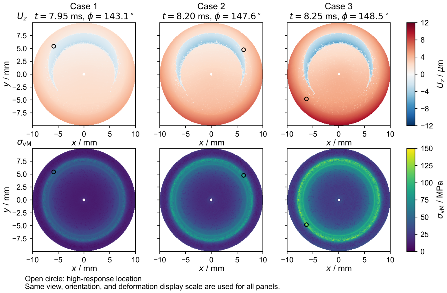
Figure 16 compares the normal deformation and von Mises stress distributions under steady-load conditions, and Table 7 summarizes the peak structural-response metrics for all seven cases. Under steady loading, increasing the load level amplifies the structural response in a nearly monotonic manner. The maximum total deformation increases from $5.59\mathsf{\mu }\mathrm{m}$ in Case 1 to $8.45\mathsf{\mu }\mathrm{m}$ in Case 2 and $11.34\mathsf{\mu }\mathrm{m}$ in Case 3. Over the same sequence, the normal deformation range increases from $8.68\mathsf{\mu }\mathrm{m}$ to $13.04\mathsf{\mu }\mathrm{m}$ and $17.47\mathsf{\mu }\mathrm{m}$, respectively. This indicates that the slipper does not respond to the thermal–mechanical load only through a rigid-body-like displacement; instead, the bottom surface develops increasingly non-uniform normal warpage as the pressure and temperature loads rise.

The stress response exhibits the same load-dependent strengthening. The maximum von Mises stress increases from $65.89\mathrm{MPa}$ in Case 1 to $102.68\mathrm{MPa}$ in Case 2 and $149.37\mathrm{MPa}$ in Case 3. The maximum principal stress increases from $79.35\mathrm{MPa}$ to $168.07\mathrm{MPa}$, whereas the minimum principal stress decreases from $-103.81\mathrm{MPa}$ to $-217.16\mathrm{MPa}$. These principal-stress extrema are used as auxiliary evidence for the tensile and compressive stress-state variation, while ${\sigma }_{\mathrm{vM},\max }$ remains the primary structural strength-response indicator.

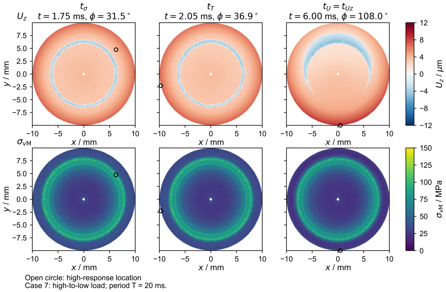
For variable-load cases, the Case 7 contour maps in Figure 17 and the time-history curves in Figure 18 further show that the structural response is path dependent and phase dependent. In Case 4, the peak values of $U_{\mathrm{total},\max }$, $U_{z,\mathrm{range}}$, and ${\sigma }_{\mathrm{vM},\max }$ are $6.95\mathsf{\mu }\mathrm{m}$, $10.77\mathsf{\mu }\mathrm{m}$, and $82.32\mathrm{MPa}$, respectively. In Case 5, these values increase to $9.81\mathsf{\mu }\mathrm{m}$, $15.16\mathsf{\mu }\mathrm{m}$, and $118.05\mathrm{MPa}$. Although Case 6 represents a large low-to-high loading command, its maximum von Mises stress is $101.61\mathrm{MPa}$, which is lower than that in Case 5. This result is consistent with the pressure and flow–thermal analyses in Section 3.1 and Section 3.3: the prescribed loading path does not guarantee that all phases within the selected cycle reach the highest instantaneous pressure level, because pressure build-up is coupled with the porting phase.

The high-to-low load case (Case 7) exhibits a particularly clear temporal separation among thermal, stress, and deformation responses. Its maximum von Mises stress reaches $129.54\mathrm{MPa}$ at $t_{\sigma }=1.75\mathrm{ms}$, while the maximum structural temperature reaches 70.34 °C at $t_T=2.05\mathrm{ms}$. In contrast, the maximum total deformation of $9.62\mathsf{\mu }\mathrm{m}$ and the maximum normal deformation range of $14.81\mathsf{\mu }\mathrm{m}$ both occur at $t_U=t_{Uz}=6.00\mathrm{ms}$. This indicates that stress and temperature peaks can precede the deformation peak during unloading, implying that the structural response is not governed only by the current pressure level but is also affected by the preceding high-load state and thermal inertia [19,22].

Overall, Figure 16, Figure 17 and Figure 18 and Table 7 show that the pressure and temperature loads transferred from the oil film generate three levels of structural response within the present single-slipper structural model. First, increasing steady load strengthens the total deformation, normal warpage, and equivalent stress. Second, variable loading changes the phase relationship among stress, temperature, and deformation peaks, especially during unloading. Third, the structural high-response location does not necessarily coincide with the highest pressure or highest temperature location in the fluid domain. These observations provide the structural evidence needed for the multi-field candidate high-risk region identification in Section 3.5.

3.5. Candidate High-Risk Region Identification Based on Cycle-Envelope Fields

The candidate high-risk region discussed in this paper does not represent a region where structural damage, film rupture, wear, yielding, or fatigue failure has already occurred. Instead, it denotes a relative high-response region jointly characterized by local film thinning, oil-film temperature-rise concentration, and structural stress concentration within a variable-load cycle. This definition is consistent with the evidence boundary of this paper. Existing mixed thermoelastohydrodynamic and lubrication–wear interaction models have incorporated asperity contact and wear evolution to evaluate degradation processes [24,25]. In contrast, this paper does not introduce absolute thresholds for oil-film rupture, material yielding, wear initiation, or fatigue life. The regions identified here should therefore be interpreted as candidate high-risk regions rather than confirmed failure regions.

To avoid identifying risk only from a single instantaneous peak, this paper uses cycle-envelope fields to define the core high-response regions. For each load case, the minimum film-thickness envelope, maximum oil-film temperature envelope, and maximum structural stress envelope are defined as

$$h_{min}^{\mathrm{cyc}}(x,y)=\underset{t}{min}h(x,y,t),$$

(20)

$$T_{max}^{\mathrm{cyc}}(x,y)=\underset{t}{max}{T}_f(x,y,t),$$

(21)

$${\sigma }_{max}^{\mathrm{cyc}}(x,y)=\underset{t}{max}{\sigma }_{\mathrm{vM}}(x,y,t).$$

(22)

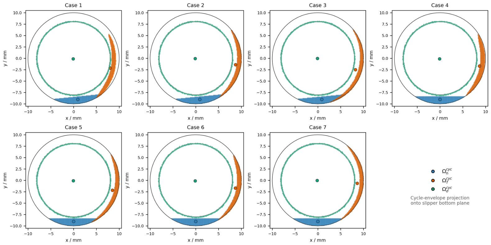
Here, $h_{min}^{\mathrm{cyc}}(x,y)$ is reconstructed from the 400-step posture history over the 0–$20\mathrm{ms}$ local cycle, $T_{max}^{\mathrm{cyc}}(x,y)$ is obtained from the 81 saved CFD oil-film temperature frames over the same cycle, and ${\sigma }_{max}^{\mathrm{cyc}}(x,y)$ is extracted from the 400-step transient structural von Mises stress field. The temperature-rise high-response region ${\mathsf{\Omega }}_T$ is defined only from the CFD oil-film temperature envelope.

The core high-response regions are identified using a relative percentile criterion. The film-thinning core region ${\mathsf{\Omega }}_h$ is defined as the lowest 10% of $h_{min}^{\mathrm{cyc}}(x,y)$, the temperature-rise core high-response region ${\mathsf{\Omega }}_T$ is defined as the highest 10% of $T_{max}^{\mathrm{cyc}}(x,y)$, and the stress core high-response region ${\mathsf{\Omega }}_{\sigma }$ is defined as the highest 10% of ${\sigma }_{max}^{\mathrm{cyc}}(x,y)$. The 10% level is an equal-area lower/upper-decile rule rather than an absolute failure criterion. Statistically, it permits a unit-independent comparison among the three fields and across load cases; physically, it confines the comparison to compact locations of the strongest film-thinning, temperature-rise, and stress responses without implying film rupture, wear, or material failure. The Jaccard overlap ratio between two regions is calculated as

$${\eta }_{ij}={\displaystyle \frac{A({\mathsf{\Omega }}_i\cap {\mathsf{\Omega }}_j)}{A({\mathsf{\Omega }}_i\cup {\mathsf{\Omega }}_j)}}.$$

(23)

In

Table 8. Cycle-envelope projection statistics and maximum pairwise Jaccard overlap ratio across seven load cases.

Case	Condition	${\mathit{\varphi }}_{\mathit{h}min}$ (°)	${\mathit{\varphi }}_{\mathit{T}max}$ (°)	${\mathit{\varphi }}_{\mathit{\sigma }}$ (°)	${\mathit{\varphi }}_{\mathbf{Uz},\mathbf{range}}$ (°)	Relation	${\mathit{\eta }}_{\mathit{J},max}$
1	Low steady	18.2	148.5	143.1	179.1	adjacent	0.0104
2	Medium steady	17.3	148.5	147.6	170.1	adjacent	0.0057
3	High steady	18.2	153.0	148.5	175.5	adjacent	0.0327
4	Low to medium	18.2	180.0	179.1	179.1	none	0.0000
5	Medium to high	17.3	157.5	175.5	175.5	adjacent	0.0101
6	Low to high	18.2	171.0	166.5	179.1	adjacent	0.0019
7	High to low	359.3	31.5	31.5	108.0	adjacent	0.0017

, ${\eta }_{J,max}$ denotes the maximum pairwise Jaccard overlap ratio among ${\mathsf{\Omega }}_h$, ${\mathsf{\Omega }}_T$, and ${\mathsf{\Omega }}_{\sigma }$. The relation grade “adjacent” indicates that no common triple-overlap core is formed, but at least two projected core regions show edge-adjacent or near-edge topology within the $0.1\mathrm{mm}$ projection grid. The grade “none” indicates that neither effective overlap nor edge adjacency is detected.

Figure 19 and Table 8 present the cycle-envelope projection results for all seven load cases. The three high-response regions are projected onto a common x–y plane in the slipper bottom coordinate system. Under the 10% criterion, the area fractions of ${\mathsf{\Omega }}_h$, ${\mathsf{\Omega }}_T$, and ${\mathsf{\Omega }}_{\sigma }$ are close to the prescribed value. More importantly, the three core high-response regions do not form a common overlap region in any case, and the pairwise overlap ratios remain within 0–$3.27\%$. Case 4 shows no effective overlap under the current $0.1\mathrm{mm}$ projection grid, whereas the other cases mainly exhibit adjacent or weakly overlapping distributions. This indicates that film thinning, oil-film temperature rise, and structural stress concentration do not collapse into a single peak location; rather, they form an edge-adjacent spatial topology [17,22].

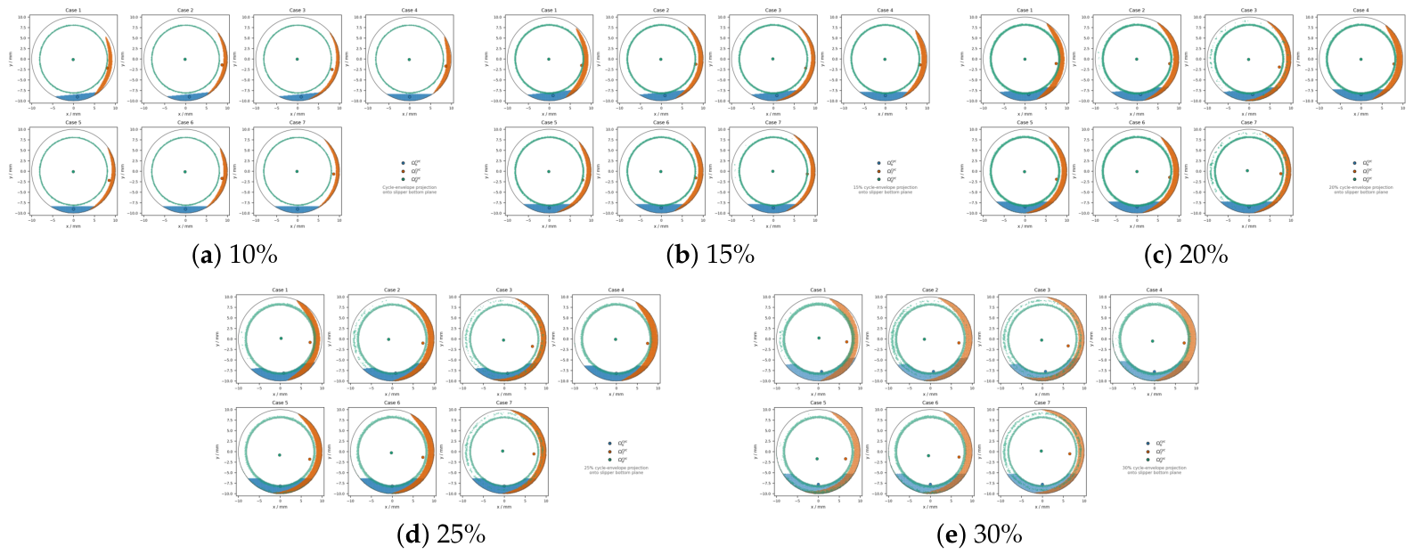
The 10% criterion is retained as the base threshold because it isolates the compact extreme-response cores defined above. In the 15–30% checks shown in Figure A2, the common triple-overlap fraction remains zero at 15%; at 20%, only Cases 3 and 7 show very small values with a maximum of $0.30\%$ of the three-region union. The maximum then increases to $1.57\%$ and $4.71\%$ at 25% and 30%, respectively, as the selected regions broaden. This expected expansion supports using 10% for core-region reporting and the larger fractions only as sensitivity bounds; none of these percentiles is interpreted as a failure threshold.

From the spatial distribution, ${\mathsf{\Omega }}_h$ is mainly located near the outer-edge film-thinning band, indicating that slipper posture and instantaneous clearance reconstruction first determine the local film-thinning location. ${\mathsf{\Omega }}_T$ is concentrated mainly on the outer-edge side of the oil film, suggesting that temperature-rise high-response regions tend to develop near regions with smaller local film thickness, larger velocity gradients, or stronger shear dissipation. ${\mathsf{\Omega }}_{\sigma }$ represents the structural stress-envelope high-response region. The full cycle-envelope source data retain auxiliary geometric quantities, including thresholds, centroid distances, and nearest projected distances, whereas the main-text Table 8 keeps only the phase values, Jaccard overlap ratios, and spatial-relation grades to avoid an excessively wide table. Thus, the structural stress high-response region is spatially associated with the film-thinning and temperature-rise high-response regions, but it is not completely co-located with them. Its formation is also affected by the pressure-load path, temperature gradient, and geometric features of the slipper body.

The temporal relationship among the three response types was evaluated by converting the characteristic instants to a local cycle phase,

$$\varphi ={\displaystyle \frac{mod(t-t_0,T)}{T}}\times {360}^{\circ },$$

(24)

where $T=20\mathrm{ms}$ and $t_0=0.20\mathrm{s}$. In Cases 1–6, ${\varphi }_{hmin}$ is concentrated around $17.3^{\circ }$–$18.2^{\circ }$, whereas ${\varphi }_{Tmax}$, ${\varphi }_{\sigma max}$, and ${\varphi }_{Uz,\mathrm{range}}$ are mainly distributed around ${143}^{\circ }$–${180}^{\circ }$. In Case 7, the response sequence is different: ${\varphi }_{\sigma max}$ and ${\varphi }_{Tmax}$ are both approximately $31.5^{\circ }$, ${\varphi }_{Uz,\mathrm{range}}$ is approximately $108.0^{\circ }$, while ${\varphi }_{hmin}$ approaches $359.3^{\circ }$. This phase separation indicates that the unloading condition is influenced by the preceding high-load state and thermal accumulation.

Overall, the formation of candidate high-risk regions under variable loading follows a chain-like transmission mechanism. The piston chamber pressure is first modulated by the damping orifices and central pocket to form the actual pressure boundary. This pressure boundary drives slipper posture evolution and reconstructs the instantaneous clearance $h(x,y,t)$. When the local film thickness decreases, the velocity gradient and shear dissipation in the oil film are enhanced, promoting localized temperature rise. The pressure and temperature fields are then transferred to the slipper structure as thermal–mechanical loads, producing non-uniform normal deformation and a local von Mises stress response. Therefore, the candidate high-risk region under variable loading should be interpreted as a relative high-response and lubrication-safety-sensitive zone. It is not determined by a single pressure peak, temperature peak, or structural stress peak but rather by the spatial proximity and phase difference among film-thinning, temperature-rise, and stress high-response regions. Based on the cycle-envelope projection, the outer-edge film-thinning band and its adjacent temperature-rise and structural stress high-response regions are identified as the main candidate high-risk region in this paper.

A principal limitation is that the present framework has not been validated against physical slipper-pair measurements; the grid- and time-step studies in Section 2.4 assess numerical sensitivity only. A staged experiment should first reproduce the same nominal low, medium, and high pressure levels at $3000\mathrm{r}/\min$ on an instrumented slipper-bearing or pump test rig. Synchronized pressure transducers for $p_{\mathrm{ct}}$ and $p_{\mathrm{ht}}$, three circumferentially spaced eddy-current film-thickness probes, and near-surface temperature sensors around the sealing land would test the predicted pressure attenuation, posture response, and azimuth of outer-edge thermal localization using established slipper-test-rig concepts [9,10]. Subsequent low-to-high and high-to-low load-transition tests, synchronized with shaft angle, should compare measured extrema and their phase order with the predicted cycle envelopes. Where feasible, strain or deformation measurements on an instrumented slipper could assess the structural-response location; post-test surface inspection should be treated only as a separate check of whether repeated response localization develops into damage. Validation should be judged by spatial location, phase order, and trends across load cases rather than by treating the current 10% criterion as an experimental failure threshold.

4. Conclusions

This paper established a sequential analysis framework for the slipper pair of an axial piston pump under variable loading. The framework links piston chamber pressure, central pocket pressure, slipper posture, instantaneous clearance, three-dimensional flow–thermal field, single-slipper structural response, and candidate high-risk region identification within a unified local cycle. The scientific contribution is threefold: (i) the central-pocket pressure boundary is resolved through dual-orifice and dual-control-volume transmission instead of directly imposing piston chamber pressure; (ii) this boundary is propagated through posture-dependent clearance to three-dimensional flow–thermal and single-slipper structural responses while retaining a common local-cycle phase reference; and (iii) candidate high-risk regions are screened from the spatial proximity and phase relationship of multiple cycle-envelope fields rather than from a single instantaneous peak. The third contribution is a comparative numerical screening method and does not constitute validation of wear, failure, or service life. The main conclusions are as follows.

First, the piston chamber pressure is not equivalent to the actual pressure boundary acting on the slipper bottom. The dual-orifice and dual-chamber pressure transmission model shows that the central pocket pressure exhibits peak attenuation, peak-time difference, and pressure-rate weakening relative to the piston chamber pressure. Under steady loading, the peak attenuation ratio of $p_{\mathrm{ht}}$ relative to $p_{\mathrm{ct}}$ is approximately $2.83$–$3.33\%$. Under variable loading, the pressure-rate weakening ratio is $6.29$–$7.14\%$, and the high-to-low load case shows the largest peak attenuation ratio of $4.81\%$. These results indicate that $p_{\mathrm{ht}}$, rather than $p_{\mathrm{ct}}$, should be used as the pressure boundary for subsequent flow–thermal and structural analyses.

Second, the pressure-driven posture response reconstructs the instantaneous clearance and changes the downstream flow–thermal behavior. With increasing steady load, the minimum film thickness increases from approximately $13.024\mathsf{\mu }\mathrm{m}$ to $13.452\mathsf{\mu }\mathrm{m}$, indicating that the slipper posture becomes more uniform within the examined steady-load range. However, the maximum oil-film temperature rise increases from $34.12\mathrm{K}$ to $65.01\mathrm{K}$. Therefore, improved film-thickness uniformity does not necessarily imply a weaker thermal response. The variable-load cases further show that local film thinning, pressure peaks, and temperature-rise peaks do not always occur synchronously within one cycle.

Third, within the single-slipper structural model, the transient structural analysis shows that the pressure and temperature fields mapped from the oil film induce total deformation, normal warpage, and von Mises stress response in the slipper body. Increasing steady load strengthens all three structural response metrics, while variable loading changes their phase relationship. In the high-to-low load case, the structural stress and temperature peaks appear earlier than the maximum total deformation and maximum normal deformation range, suggesting that structural response during unloading is affected by the preceding high-load state and thermal inertia.

Fourth, the cycle-envelope projection demonstrates that the film-thinning, temperature-rise, and stress core high-response regions do not form a common overlap region under the 10% criterion. The pairwise Jaccard overlap ratios remain within 0–$3.27\%$. This indicates that the candidate high-risk region is better identified through the spatial proximity and phase relationship among multiple physical fields rather than through a single peak value. The outer-edge film-thinning band and its adjacent temperature-rise and structural stress high-response regions are identified as the main candidate high-risk region, which is interpreted as a relative high-response and lubrication-safety-sensitive zone in the present analysis.

For practical design use, the framework is best applied as a comparative screening workflow rather than as a direct optimization rule. Under the same duty cycle, engineers can rerun the pressure-transmission–posture–clearance–flow–thermal–structural chain for candidate damping-path or slipper-geometry variants and compare central-pocket pressure modulation, minimum film thickness and uniformity, temperature rise, deformation, stress, and the spatial relation among the corresponding high-response regions. The outer sealing-land/edge neighborhood identified here is therefore a priority region for evaluating candidate designs and planning measurements. However, because no geometry sensitivity or optimization was performed, the present results do not prescribe a universal increase or decrease in orifice size, pocket or land dimensions, or nominal clearance. Similarly, only ZQSn10-1 was analyzed; material screening would require dedicated comparative calculations with candidate-specific thermal and mechanical properties and a justified heat-transfer boundary followed by separate tribological and experimental assessment. No material superiority is inferred from the current model.

This paper does not predict the wear amount, oil-film rupture, material yielding, or fatigue life. The candidate high-risk regions identified here are relative high-response regions defined by cycle-envelope projection and percentile thresholds. The pressure-transmission model is also single-phase and does not resolve dissolved-air release or cavitation mass transfer; low-pressure cavitation onset remains outside the present scope. Variations of density, specific heat capacity, and thermal conductivity with pressure and temperature are likewise neglected, and the influence of this constant-property assumption should be quantified in future sensitivity studies. The viscosity-model form was not calibrated against oil-specific high-pressure rheometry or benchmarked against a Roelands relation; its use is therefore restricted to the present pressure–temperature envelope, and model-form sensitivity should be assessed when suitable high-pressure viscosity data become available. The fluid-side adiabatic wall was not benchmarked against a conjugate heat-transfer solution. Although transient conduction inside the bronze slipper was solved downstream from mapped surface temperatures, the corresponding interfacial heat flux was not fed back to Fluent. The absolute oil-film temperature and thermally induced structural response are therefore boundary-conditioned. Future work should close the interfacial energy balance through partitioned temperature–heat-flux iteration or fully conjugate fluid–solid heat transfer. No physical slipper-pair experiment was performed, and the numerical sensitivity studies do not substitute for experimental validation. The staged steady-state and load-transition measurements outlined in Section 3.5 would be required before the predicted spatial locations and phase relations can be regarded as experimentally confirmed. Future work should incorporate surface roughness, asperity contact, wear evolution, absolute critical thresholds, and experimental validation to further connect the present candidate-region identification method with quantitative degradation and life prediction.

References

1. Pang, Z.; Zhai, W.; Shun, J. The study of hydrostatic lubrication of the slipper in a high-pressure plunger pump. Tribol. Trans. 1993, 36, 316–320. [Google Scholar] [CrossRef] [Scilit]
2. Xu, B.; Li, Y.B.; Zhang, B.; Zhang, J.H. Numerical simulation of overturning phenomenon of axial piston pump slipper pair. J. Mech. Eng. 2010, 46, 161–168. [Google Scholar] [CrossRef] [Scilit]
3. Wang, Y.J. Calculation method of lubricant film pressure distribution of axial piston pump slippers. Appl. Mech. Mater. 2013, 328, 629–633. [Google Scholar] [CrossRef] [Scilit]
4. Wang, Q.N.; Xu, B.; Zhang, J.H. Optimization design of the inner radius of the sealing surface of slipper. In Proceedings of the 2015 IEEE International Conference on Advanced Intelligent Mechatronics (AIM), Busan, Republic of Korea, 7–11 July 2015; pp. 388–395. [Google Scholar] [CrossRef] [Scilit]
5. Guan, D.; Cong, X.; Li, J.; Niu, Z. Experimental test and theoretical modeling on the working characteristics of spherical water pump. Flow Meas. Instrum. 2022, 85, 102162. [Google Scholar] [CrossRef] [Scilit]
6. Du, Y.; Zhao, H.; Ji, H.; Wang, W.; Xu, F.; Wang, H. Research on leakage characteristic of slipper pair of aviation piston pump considering viscosity temperature and pressure effect. Proc. Inst. Mech. Eng. Part J J. Eng. Tribol. 2026, 240, 1065–1075. [Google Scholar] [CrossRef] [Scilit]
7. Meng, X.; Ge, C.; Liang, H.; Lu, X.; Ma, X. Lubrication characteristics of the slipper–swash-plate interface in a swash-plate-type axial piston pump. Proc. Inst. Mech. Eng. Part C J. Mech. Eng. Sci. 2021, 235, 639–651. [Google Scholar] [CrossRef] [Scilit]
8. Ye, S.; Sun, Y.; Zhang, J.; Chen, J.; Xu, B.; Zhao, S.; Liu, H. A new coupled dynamic model to study the vibration and lubrication characteristics of slipper/swash-plate interface in an axial piston pump. Proc. Inst. Mech. Eng. Part J J. Eng. Tribol. 2025, 239, 1026–1049. [Google Scholar] [CrossRef] [Scilit]
9. Chao, Q.; Zhang, J.; Xu, B.; Wang, Q.; Huang, H. Test rigs and experimental studies of the slipper bearing in axial piston pumps: A review. Measurement 2019, 132, 135–149. [Google Scholar] [CrossRef] [Scilit]
10. Zhou, J.; Zhou, J.; Jing, C. Experimental research on the dynamic lubricating performance of slipper/swash plate interface in axial piston pumps. Chin. J. Mech. Eng. 2020, 33, 25. [Google Scholar] [CrossRef] [Scilit]
11. Lai, R.; Zhu, X.; Quan, Y.; Miao, K.; Ye, S.; Bao, Y.; Liu, H.; Zhao, S. Research on vibration and lubrication characteristics of piston pumps with coupled slipper pair and valve plate pair interactions. China Mech. Eng. 2026, 37, 275–284. [Google Scholar] [CrossRef]
12. Li, R.; Li, D.; Li, Z.; Wu, T.; Xu, J. Research on the effect of damping grooves on the pressure and cavitation characteristics of axial piston pumps. Processes 2025, 13, 1274. [Google Scholar] [CrossRef] [Scilit]
13. Li, J.; Xiong, Z.; Liu, Z.; Liu, D.; Liu, X.; Li, H. Three-dimensional modeling-driven AMESim virtual prototype development and flow characterization of swashplate axial piston pumps. J. Phys. Conf. Ser. 2025, 3024, 012011. [Google Scholar] [CrossRef] [Scilit]
14. Zhu, J.; Li, H.; Liu, J.; Fu, J. Research on dynamic lubrication characteristics of slipper pair in aviation fuel piston pump based on CFD internal flow coupling simulation. J. Propuls. Technol. 2019, 40, 1370–1381. [Google Scholar] [CrossRef]
15. Ma, J.; Li, Q.; Shen, Y. CFD-based analysis of oil-film characteristics of the swash-plate/slipper pair. J. Beijing Univ. Aeronaut. Astronaut. 2016, 42, 265–272. [Google Scholar] [CrossRef]
16. Jia, Z.; Yang, Y.; Zhao, J.; Shi, M. Research on multi-field coupling characteristics of slipper pair based on CFD. J. Dyn. Control 2023, 21, 72–80. [Google Scholar] [CrossRef]
17. Muzzioli, G.; Orlandi, F.; Venturelli, M.; Milani, M.; Montorsi, L. CFD simulation of the slipper dynamics during variable displacement operations in a swash-plate type axial piston pump. Int. J. Thermofluids 2024, 24, 100992. [Google Scholar] [CrossRef] [Scilit]
18. Tang, H.; Yin, Y.; Ren, Y.; Xiang, J.; Chen, J. Impact of the thermal effect on the load-carrying capacity of a slipper pair for an aviation axial-piston pump. Chin. J. Aeronaut. 2018, 31, 395–409. [Google Scholar] [CrossRef] [Scilit]
19. Hashemi, S.; Friedrich, H.; Bobach, L.; Bartel, D. Validation of a thermal elastohydrodynamic multibody dynamics model of the slipper pad by friction force measurement in the axial piston pump. Tribol. Int. 2017, 115, 319–337. [Google Scholar] [CrossRef] [Scilit]
20. Yun, Z.; Li, S.; Li, F.; Wang, K.; Fu, L.; Ru, C. A novel model for the thermoelastic hydrodynamic lubrication characteristics of the slipper pair in radial piston pumps. Phys. Fluids 2025, 37, 022105. [Google Scholar] [CrossRef] [Scilit]
21. Schenk, A.; Ivantysynova, M. A transient thermoelastohydrodynamic lubrication model for the slipper/swashplate in axial piston machines. J. Tribol. 2015, 137, 031701. [Google Scholar] [CrossRef] [Scilit]
22. Tang, H.; Ren, Y.; Xiang, J. Fully-coupled thermomechanical analysis for sliding contact between textured slipper and swashplate in axial piston pump. Int. J. Heat Mass Transf. 2020, 163, 120521. [Google Scholar] [CrossRef] [Scilit]
23. Ma, C.; Yan, P.; Wang, B.; Gao, L.; Liu, S.; Du, J.; Feng, L. Research on dynamic response characteristics and wear mechanism of the slipper of key friction pair in axial piston pump. Eng. Fail. Anal. 2025, 182, 109994. [Google Scholar] [CrossRef] [Scilit]
24. Dong, Z.; Liu, M.; An, H.; Guo, S.; Jin, Z.; Lin, H.; Ai, C.; Jiang, Y. Research on lubrication-wear dynamic interaction model of slipper pair under multiple working conditions. J. Tribol. 2025, 147, 121706. [Google Scholar] [CrossRef] [Scilit]
25. Liu, X.; Liu, J.; Du, T.; Liu, Y.; Guo, C.; Fu, J. Investigation of transient mixed thermoelastohydrodynamic lubrication and wear coupled characteristics at the slipper/swash plate interface in aviation fuel piston pump. Tribol. Int. 2026, 214, 111223. [Google Scholar] [CrossRef] [Scilit]
26. Li, S.; Yang, L.; Li, X.; Chen, S.; Zhang, Z. Simulation of strength and friction of slipper pair in high speed axial piston pump. Mach. Tool Hydraul. 2025, 53, 139–145. [Google Scholar] [CrossRef]
27. Dench, J.; di Mare, L.; Morgan, N.; Wong, J.S.S. Comparing the molecular and global rheology of a fluid under high pressures. Phys. Chem. Chem. Phys. 2018, 20, 30267–30280. [Google Scholar] [CrossRef] [Scilit] [PubMed]
28. Muzzioli, G.; Paltrinieri, F.; Montorsi, L.; Milani, M. A computation fluid dynamics methodology for the analysis of the slipper-swash plate dynamic interaction in axial piston pumps. Fluids 2023, 8, 246. [Google Scholar] [CrossRef] [Scilit]
Figure 1. Sequential coupling framework for slipper-pair transient response and candidate high-risk region identification under variable loading. CFD, computational fluid dynamics; UDF, user-defined function; P/T, pressure/temperature.
Lubricants 14 00285 g001
Figure 2. System-level variable-load boundary model and transient input extraction. LS, load sensing; LSC, load-sensing controller; PCV, pressure-compensating valve.
Lubricants 14 00285 g002
Figure 3. Double-throttle and dual-control-volume pressure transmission path from the piston chamber to the slipper oil film.
Lubricants 14 00285 g003
Figure 4. Posture-based film-thickness reconstruction and polar finite-difference discretization of the slipper oil film.
Lubricants 14 00285 g004
Figure 5. Force balance and hydrostatic support decomposition of the piston–slipper assembly.
Lubricants 14 00285 g005
Figure 6. Typical-cycle pressure transmission histories under steady load conditions.
Lubricants 14 00285 g006
Figure 7. Pressure transmission during single-cycle variable-load transitions.
Lubricants 14 00285 g007
Figure 8. Cross-case comparison of pressure attenuation, peak-time difference and rate weakening.
Lubricants 14 00285 g008
Figure 9. Steady-load posture histories over one rotation period.
Lubricants 14 00285 g009
Figure 10. Steady-load film-thickness reconstruction and posture uniformity metrics.
Lubricants 14 00285 g010
Figure 11. Posture response during single-cycle variable-load transitions. The annotations report Δ t p = t d t p and Δ t h = t d t h . Blue dashed, orange dotted, and green dashed vertical lines denote the pressure-peak, central-film-thickness-minimum, and local-film-thickness-minimum instants, respectively.
Lubricants 14 00285 g011
Figure 12. Minimum-film-thickness-instant reconstruction and phase relation during variable-load transitions. L, low; M, medium; H, high.
Lubricants 14 00285 g012
Figure 13. Pressure and temperature-rise fields of steady load cases at 90-degree phase.
Lubricants 14 00285 g013
Figure 14. Pressure and temperature-rise fields of variable-load cases at 180-degree phase.
Lubricants 14 00285 g014
Figure 15. Full-domain maximum temperature-rise evolution showing thermal inertia and path dependence across seven load cases: (a) heatmap; (b) waterfall plot. Circular markers identify the maximum temperature-rise instant of each case (white in panel (a) and case-colored in panel (b)).
Lubricants 14 00285 g015
Figure 16. Steady-load normal deformation and von Mises stress distributions at peak structural stress.
Lubricants 14 00285 g016
Figure 17. Critical-instant structural response under the high-to-low load condition. Open circles mark the high-response locations at the three selected instants.
Lubricants 14 00285 g017
Figure 18. Structural-response time histories across seven load cases: (a) maximum total deformation; (b) normal deformation range; (c) maximum structural temperature; (d) maximum von Mises stress.
Lubricants 14 00285 g018
Figure 19. Cycle-envelope projection of candidate high-risk regions across seven load cases.
Lubricants 14 00285 g019