Method for Real-Time Monitoring of the Lubrication Regimes in Dynamically Loaded Radial Sliding Bearings Using Physics-Informed Neural Networks (PINNs)

Abstract

This study proposes a model-based method for real-time monitoring of the lubrication regimes in dynamically loaded radial sliding bearings using Physics-Informed Neural Networks (PINN). The proposed method replaces computationally intensive elastohydrodynamic lubrication (EHD) simulations with a PINN-based surrogate model. The model predicts hydrodynamic pressure and lubricant film-thickness distributions with comparable accuracy under dynamically varying operating conditions, enabling reliable assessment of lubrication regimes. The proposed model advances the state of the art in physics-informed modelling of mixed lubrication by extending existing approaches to simultaneously account for mixed-friction regimes through the Greenwood–Tripp contact model, transient operating conditions, and bearing surface deformation. Using only the bearing load and shaft rotational speed as inputs, the resulting hydrodynamic pressure field and corresponding lubricant film thickness can be monitored, enabling the direct assessment of the lubrication regime and potential wear risk. The proposed method is applied to a validated EHD model of a 30 mm sliding bearing test rig, where EHD simulation results are used to train, validate, and evaluate the model. The proposed framework achieved an average lubricant film-thickness prediction error of 2.34% and lubrication-regime classification errors of 7.8% and 8.2% for the static and dynamic validation cases, respectively. Furthermore, the computation time for the complete 18-time-step load case was reduced from approximately 35 h to 61.2 ms.

1. Introduction

Radial sliding bearings are widely employed in a variety of technical applications that face challenging operating and environmental conditions, such as wind turbine gearboxes, internal combustion engines and marine propulsion systems [1,2,3]. Despite their widespread use, sliding bearings are often identified as a critical source of failure, with wear-related damage accounting for approximately 80% of failures [4]. These wear mechanisms are strongly influenced not only by operating conditions but also by the combination of lubricant properties and bearing material properties. Lubricant viscosity governs the formation of the lubricant film, while the bearing material affects both the wear rate and the dominant wear mechanisms [5]. For example, an increased incidence of wear-related failures in marine stern tube bearings has been reported after replacing mineral oils with environmentally acceptable lubricants (EALs) [6,7]. Furthermore, white metal bearings are generally more susceptible to wiping under high loads and temperatures, whereas bronze bearings are more prone to adhesive wear [5,7]. Consequently, wear-related damage can significantly undermine system reliability, increase maintenance costs, and lead to economic losses. Therefore, preventing such failures requires satisfying the film-thickness criterion, which states that the minimum lubricant film thickness must exceed a critical threshold defined by the combined surface roughness of the shaft and bearing [8,9]. The criterion specifies a minimum film height to prevent mixed lubrication, which would otherwise cause wear and potential failure. Since the film thickness of sliding bearings is highly dependent on operating conditions, which vary dynamically in most applications, continuous monitoring of the film thickness is essential [10,11]. Monitoring oil film thickness enables the identification of early changes in the contact or lubrication regime that could lead to wear risk [11]. Based on this identification, the operating strategy can be proactively adapted to ensure reliable and safe bearing operation while preventing escalation to severe failures, such as adhesive wear [5,12,13].

Two primary approaches to monitoring exist: physical sensing and model-based approaches [11]. Physical sensors, such as temperature, vibration, and acoustic emission (AE) sensors, are often associated with high hardware costs, complex installation requirements, and demanding signal-processing techniques [14,15]. In certain applications, such as marine propulsion systems and internal combustion engines, physical sensor installations may be restricted or impractical [2]. As an alternative, model-based approaches employ mathematical models to predict system behaviour, reducing dependence on physical sensors while improving system reliability and reducing hardware costs [14]. However, for model-based approaches, applicability depends on the accuracy of the mathematical modelling and calculation time, since the calculations must be performed in real time.

The definition of ‘real-time’ varies across applications, influenced by the specific purpose of the monitoring [12,13]. When optimising operational strategies directly, real-time data on the scale of seconds are required [12,14]. Such rapid feedback enables immediate corrective actions, enhances reliability, and effectively prevents failures [12,14]. Similar to the requirements for real-time-capable simulation models, the required fidelity varies by application, depending on the loading complexity. High-fidelity approaches are required to capture the complex interactions among load, structural deformation, and lubrication, especially in heavy-duty systems such as marine propulsion systems, wind turbine gearboxes, and internal combustion engines [1,3,16]. In such cases, EHD simulations are commonly employed [6,16,17]. These numerical EHD simulations capture lubrication and contact conditions, such as oil film thickness and hydrodynamic pressure, under the influence of load and deformation, thereby providing a reliable and accurate basis for bearing performance assessment [6,16,17]. Although EHD-based approaches accurately capture lubrication behavior, their numerical solution is computationally demanding [18]. The required computational effort grows considerably when these models are embedded within multibody system (MBS) simulations that incorporate elastic deformation and mixed lubrication effects [11]. This makes EHD simulations unsuitable for the real-time monitoring applications [19]. Therefore, high-fidelity models capable of operating in real time are needed.

Existing model-based approaches for real-time monitoring can be broadly categorized as physics-based, data-driven, or hybrid [20,21,22,23]. Physics-based approaches, also called white box approaches, encompass analytical and empirical models whose simplified formulations enable efficient implementation with relatively low computational effort. However, they typically offer limited fidelity, are restricted to rigid systems and steady-state radial loading, and neglect effects such as surface roughness and misalignment [19]. Addressing these effects requires computationally expensive time-dependent and multiscale models, reducing the practicality of this approach [24,25]. As an alternative, correction factors are often introduced to account for neglected effects; however, they are usually derived for specific conditions and valid only within limited ranges [19,26]. Thus, the simplifications and assumptions used in their development limit the predictive accuracy of white-box approaches [26].

Data-driven approaches, often based on machine learning (ML) and commonly referred to as black-box models, use experimental or simulation data to provide real-time predictions without explicit knowledge of the underlying physical system [27]. The rapid adoption of machine learning in tribology has been comprehensively reviewed by Argatov et al. [28], Rosenkranz et al. [29], Marian et al. [30], Sose et al. [31] and Paturi et al. [32]. For instance, Marian et al. [33] employed machine learning approaches to predict film-thickness parameters. To estimate wear volume in journal bearings subjected to start–stop operation, König et al. [34] evaluated different neural network architectures for time-series forecasting, including LSTM, GRU, and NARX. Despite their rapid development in recent years, purely data-driven approaches remain highly dependent on the quality and quantity of the available training data [28,29,30,31,32,35]. Moreover, they often exhibit limited generalisation and transferability beyond the conditions encountered during training [36]. Furthermore, relying solely on purely data-driven models may lead to physically implausible predictions, such as negative lubricant film thickness [19,36].

Building on these two modelling approaches, white box and black box, a third category known as grey box approaches has emerged in recent years [37]. This hybrid approach, often referred to as Scientific Machine Learning (SciML), combines the interpretability of physics-based models with the adaptability of machine learning models [27,36]. Several techniques have been developed in this direction, including physics-guided machine learning, reduced-order models with embedded physics, and Physics-Informed Neural Networks (PINNs) [36,37,38]. Among these, PINNs have emerged as a promising framework capable of overcoming many of these limitations [36,37,38]. Within PINNs, the term framework refers to the combined structure of the neural network, governing the physical equations, loss formulation, and training strategy. The primary advantage of PINNs lies in their ability to integrate the governing Partial Differential Equation (PDE) directly into neural network training [11]. This integration improves data efficiency, ensures physically consistent predictions, and enables generalisation even with limited or noisy data [36]. Unlike white box models, PINNs can efficiently handle complex nonlinear systems once they are trained [36,39]. At the same time, PINNs overcome the main limitation of black-box models by reducing the dependence on large datasets through embedded physical laws and, in some cases, can operate entirely without data [36,40].

The potential of PINNs in tribology was first demonstrated by Almqvist et al. [41], who applied the approach to solve a simplified one-dimensional Reynolds equation for an incompressible and isoviscous fluid in a linear slider bearing. Since then, PINNs have been increasingly applied in tribology, accompanied by a growing number of related publications. An overview of representative studies, particularly those addressing sliding bearings, is provided in

Table 1. Overview of PINN Applications for Sliding Bearings in the Literature.

Year	Authors	Activation Functions	Layers/Neurons Number	NN Family	Inputs	Output	Domains	Operating Regime
2021	Almqvist [41]	Sigmoid	1/10	FF-NN	x	p	1D/ Rigid	Static
2023	Zhao [45]	Sigmoid	3/16	FF-NN	x, y	p	2D/ Rigid	Static
2023	Rom [40]	Tanh	6/20	CNN	x, y and x, y, ε	p, θ	2D/ Rigid	Static
2023	Cheng [46]	ReLU-square, Tanh	6/20	FF-NN	x, y	p, θ	2D/ Rigid	Static
2023	Ramos [42]	Tanh	6/15–60	MLP	x, y, ε, φ, ėX, ėY	p	2D/ Rigid	Dynamic (excluding transient effects, e.g., squeeze-film effect)
2024	Shutin [43]	Tanh	10/20	FF-NN	x, y, u, v	p	2D/ Rigid	Dynamic (excluding transient effects, e.g., squeeze-film effect)
2024	Zhou [47]	Tanh	3/32	FF-NN	x, y	p	2D/ Rigid	Static
2025	Saleh [11]	Sigmoid, softplus	4/256	FF-NN	z, θ, F, n	p, h	2D/ Flexible	Static
2026	Hou [44]	ReLU-square, Sigmoid	6/20	MLP	x, y, F, n	p, ε	2D/ Rigid	Static

. The reviewed studies indicate the potential of PINNs for solving the computationally intensive Reynolds equation in hydrodynamic radial sliding bearings, with promising results compared to conventional simulations. Most existing studies focus on solving the quasi-static Reynolds equation to estimate the hydrodynamic pressure within the fully hydrodynamic regime, typically at a single operating point. Recently, Ramos et al. [42] and Shutin et al. [43] applied PINNs to the quasi-static Reynolds equation in rotor-dynamic analyses by using internal physical quantities as inputs, including shaft eccentricity, journal centre position, and velocities, to predict the pressure distribution. However, these approaches neglect transient effects, including squeeze-film phenomena, and rely on internal variables such as shaft eccentricity parameters, which are not directly accessible and therefore require additional sensors or estimation models based on predefined assumptions. More recently, Saleh et al. [11] proposed a PINN-based monitoring approach for sliding bearings that predicts lubricant film thickness and hydrodynamic pressure from measurable operating parameters, such as rotational speed and bearing load. However, the model is limited to static operating conditions and neglects bearing deformation as a direct physical constraint, as well as the mixed-friction regime. Building upon the approach proposed by Saleh, Hou [44] extended the methodology to include consideration of the mixed-friction regime based on the Greenwood & Tripp contact model. However, this extension relies on hard constraints and partially decoupled networks, which impose a rigid geometry and prevent full two-way coupling between pressure and film thickness.

In summary, existing studies have demonstrated the potential of PINNs for solving the computationally intensive Reynolds equation, achieving promising agreement with numerical simulations. However, the current state of research on PINN-based applications for sliding bearings remains constrained by several limitations. In particular, existing studies often neglect one or more relevant physical effects and do not consider them simultaneously:

• Assumption of a rigid bearing model and neglect of elastic deformation effects.
• Assumption of a prescribed film thickness, requiring the film thickness to be provided in advance.
• Reliance on the quasi-static Reynolds equation, neglecting the time-dependent film thickness term and potentially failing to capture transient loading behaviour such as squeeze-film effects
• Neglect of mixed-friction regimes and associated contact models to account for asperity contact pressure, which is essential for bearing force balancing.

This study addresses these limitations simultaneously by extending the framework proposed by Saleh [11]. The proposed extension explicitly accounts for mixed-friction regimes using the Greenwood & Tripp contact model, dynamic operating conditions including transient effects, and bearing surface deformation as physical constraints [48,49,50,51]. Using only the bearing load and shaft rotational speed as inputs, the proposed method replaces time-intensive EHD simulations with a PINN-based surrogate model that predicts local hydrodynamic pressure and film thickness distributions. Using the film thickness and the lubrication regime, the mixed friction can be determined. As an application case study, a validated EHD model of a 30 mm radial sliding bearing test rig is used to generate the training and validation datasets. Beyond addressing these modelling limitations, the proposed framework is not intended to replace conventional EHD solvers for offline analyses. Instead, it enables real-time prediction of the lubrication state for integration into condition monitoring, control, and digital engineering workflows.

2. Materials and Methods

The development of the proposed PINN framework is described in the following sections. First, the EHD model together with the simulation procedure used to produce the training and validation datasets is introduced in Section 2.1. Section 2.2 then describes the PINN architecture and its implementation for rapid prediction of hydrodynamic pressure and lubricant film thickness, providing the foundation for real-time lubrication regime monitoring in radial sliding bearings.

2.1. EHD Simulation

EHD simulations are formulated as coupled hydrodynamic-lubrication and elastic-deformation problems and solved iteratively until convergence. The hydrodynamic behaviour is governed by the Reynolds equation, which describes the pressure distribution within the lubricant film. The Reynolds equation proposed is expressed as follows:

$${\displaystyle \frac{\partial }{\partial x}}\left({\varphi }_x{h}^3{\displaystyle \frac{\partial p}{\partial x}}\right)+{\displaystyle \frac{\partial }{\partial y}}\left({\varphi }_y{h}^3{\displaystyle \frac{\partial p}{\partial y}}\right)=6\eta {\varphi }_s{\displaystyle \frac{\partial U}{\partial h}}{\displaystyle \frac{\partial h}{\partial x}}+12\eta {\displaystyle \frac{\partial h}{\partial t}}$$

(1)

Within Equation (1), the spatial domain is described by the coordinates x and y, corresponding to the length and width directions, respectively, while the lubricant film thickness h depends on both coordinates. The hydrodynamic pressure is represented by p, U denotes the sliding velocity, and η is the lubricant’s dynamic viscosity. The symbols ϕ_x, ϕ_y and ϕ_s refer to the pressure and shear flow factors introduced by Patir and Cheng [52,53]. The Patir and Cheng pressure and shear flow factors assume Gaussian surface roughness. Although non-Gaussian flow factor formulations have been proposed for engineering surfaces (e.g., Leighton et al. [54]; Tang et al. [55]), the classical Gaussian-based formulation remains widely used. Therefore, the Patir and Cheng flow factors are employed in this study to maintain consistency with the validated EHD/MSB model used to generate the training data.

Under high hydrodynamic pressures, elastic surface deformation becomes significant, leading to pronounced variations in film thickness that, in turn, affect the pressure distribution [56,57]. This necessitates considering and coupling hydrodynamic lubrication and elastic deformation, which can be treated either as a quasi-static coupling or as a fully dynamic one [57]. Quasi-static coupling assumes instantaneous elastic equilibrium and can be implemented through direct coupling with FEM or simplified approaches based on semi-infinite elastic body theory, such as the Boussinesq solution [56,58]. In contrast to quasi-static coupling, dynamic coupling explicitly accounts for inertia and transient structural behaviour, as implemented in multibody simulations (MBS), where Newton’s equations of motion are solved [57].

Once the Reynolds equation is solved iteratively, accounting for elastic deformation, the resulting bearing forces are then obtained by integrating the hydrodynamic pressure over the bearing surface, as expressed in Equations (2) and (3) [59,60]. In Equations (2) and (3), F denotes the force components acting in the x and y directions and P_Total(θ, z) denotes the resulting pressure field. In the fully hydrodynamic regime, P_Total(θ, z) corresponds solely to the hydrodynamic pressure, whereas in mixed-lubrication regimes, it is composed of both hydrodynamic and asperity contact pressure contributions [61]. Convergence is evaluated by comparing the computed bearing force with the applied load F.

$$F_x={\int }_0^{2\pi }{\int }_{-{\displaystyle \frac{L}{2}}}^{{\displaystyle \frac{L}{2}}}{P}_{Total}\left(\theta ,z\right)· \mathit{cos}\theta ·d\theta dz$$

(2)

$$F_y={\int }_0^{2\pi }{\int }_{-{\displaystyle \frac{L}{2}}}^{{\displaystyle \frac{L}{2}}}{P}_{Total}\left(\theta ,z\right)· \mathit{sin}\theta ·d\theta dz$$

(3)

Under mixed-lubrication conditions, the asperity contact pressure is evaluated using the stochastic Greenwood–Tripp (GT) contact mode [62]. This formulation assumes contact between nominally flat rough surfaces with random asperity distributions, from which the asperity contact pressure is obtained as follows [61]:

$$p_a=K{E}^{*}{F}_{{\displaystyle \raisebox{1ex}{$5$}\!\left/ \!\raisebox{-1ex}{$2$}\right.}}\left(H_s\right)$$

(4)

Here, K represents the elastic factor, which can be interpreted as an effective stiffness parameter of the contact model and E* is the composite elastic modulus, defined as [61]:

$$E^{*}={\left({\displaystyle \frac{1-{\upsilon }_1^2}{E_1}}+{\displaystyle \frac{1-{\upsilon }_2^2}{E_2}}\right)}^{-1}$$

(5)

where υ_i and E_i denote the Poisson’s ratio and Young’s modulus of the contacting surfaces, respectively. The function F_5/2(H_s) is the form function, defined as follows [61]:

$$F_{{\displaystyle \raisebox{1ex}{$5$}\!\left/ \!\raisebox{-1ex}{$2$}\right.}}\left(H_s\right)=\left\{\begin{array}{cc}4.4086 \times {10}^{-5}{(4-H_s)}^{6.804}, \hfill & H_s<4\hfill \\ 0,\hfill & H_s\ge 4\hfill \end{array}\right.$$

(6)

Here, H_s denotes the dimensionless clearance parameter, obtained by normalizing the local film thickness with the combined surface roughness [61].

2.1.1. EHD Model for Radial Sliding Bearing

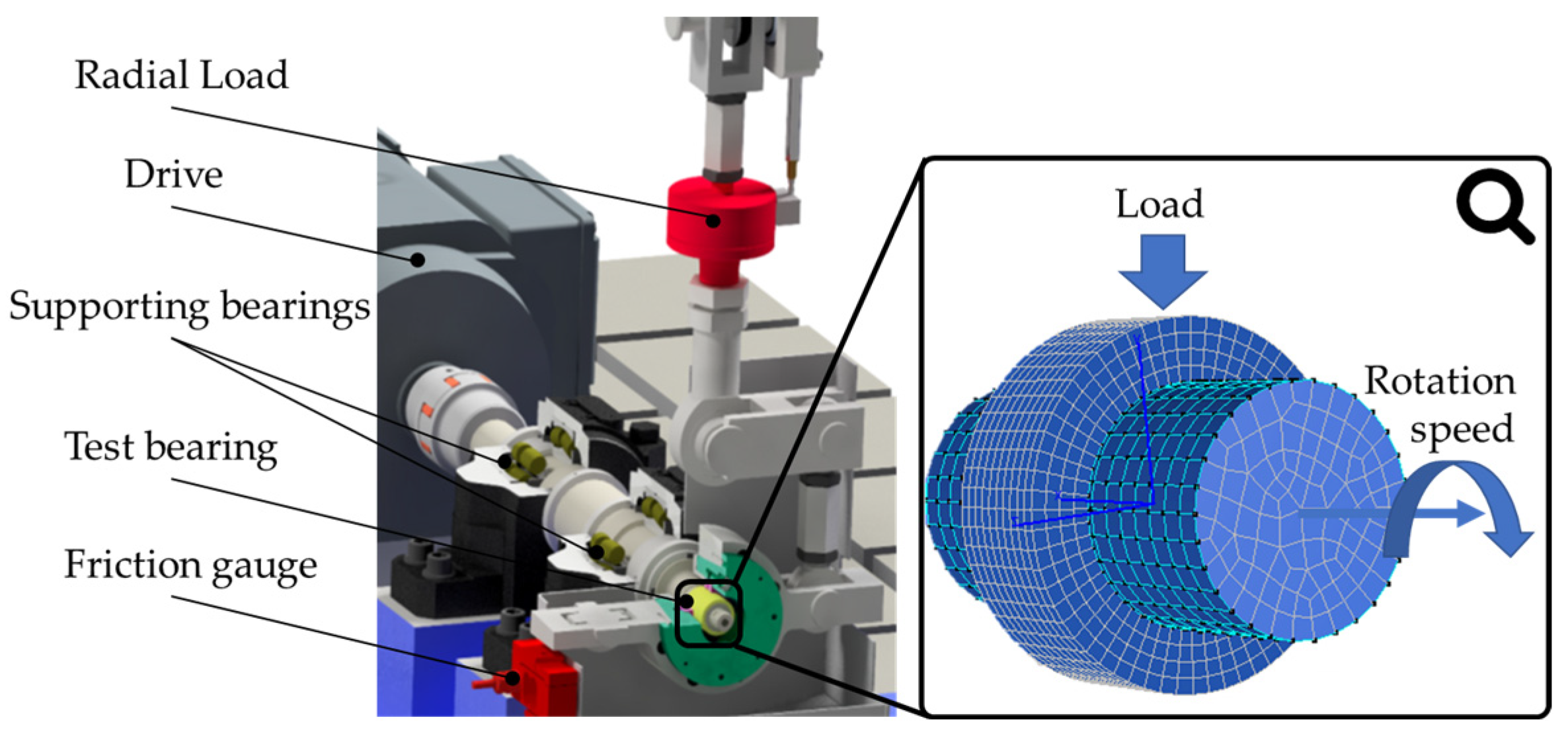
The reference EHD simulations were performed with the commercial software AVL Excite Power Unit (R2022.1). A validated EHD model of a test rig incorporating a radial sliding bearing with a diameter of 30 mm was adopted as the reference case in this study, as shown in Figure 1. This model corresponds to the test rig configuration presented by König [34,63,64,65]. The EHD model was experimentally validated by König in two independent studies [63,64,65]. Simulation inputs were divided into fixed parameters, including lubricant, geometric, material, and surface-roughness properties, and variable parameters, such as load and sliding speed, as summarised in

Table 2. Summary of simulation parameters [11].

Fixed input parameter	Lubrication	Lubricant	FVA2 (additive-free mineral oil)
		Kinematic viscosity at 40 °C	32 mm2/s
		Temperature	40 °C
	Geometry	Diameter	30 mm
		Width	15 mm
		Radial clearance	25 μm
	Bearing	Material	CuSn12Ni2-C
		Young’s modulus	108 GPa
		Poisson ratio	0.33
		Roughness Rq	0.74 μm
	Shaft sleeve	Material	AISI 52100 (100Cr6)
		Young’s modulus	210 GPa
		Poisson ratio	0.3
		Roughness Rq	0.45 μm
Variable input parameter		Radial load	0.45–5.40 kN
		Sliding speed	0.1–8 m/s

.

2.1.2. EHD Simulation Cases

As previously mentioned, one of the objectives of this work is to incorporate the dynamic effects of operating parameters alongside their static influences on lubrication and contact behaviour. Therefore, simulations under both static and dynamic operating conditions were considered in this study. For static operating conditions, 204 simulation cases were conducted to cover a range of operating points. In contrast, for dynamic conditions, 21 scenarios were simulated, each over two revolutions at varying speeds and loads. These simulations cover sliding speeds ranging from 0.1 m/s to 8 m/s and radial loads from 0.45 to 5.45 kN, corresponding to mean specific pressures between 1 and 12 MPa. Dynamic operating phases at zero or near-zero rotational speeds were not simulated due to numerical instabilities and the high computational cost, with single simulations requiring up to one week. Moreover, the initial phase corresponding to the first time step was excluded from the dataset, since transient shaft displacement effects dominate it. These effects result from the MBS initialisation procedure, which is a standard numerical treatment and does not represent the actual physical operating condition, potentially affecting the stability and consistency of the data. The datasets obtained from the EHD simulations were categorised into training, validation, and test cases, as described in Section 2.2.4.

2.2. PINNs Framework

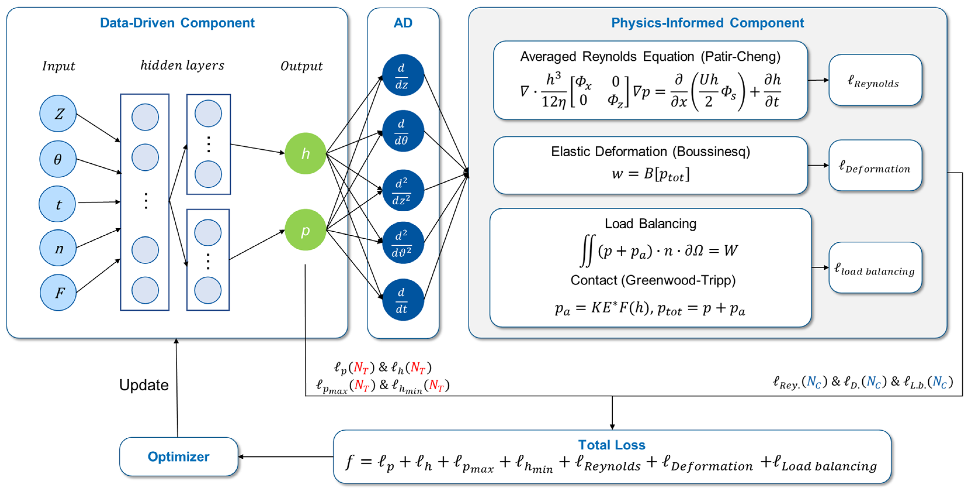
Figure 2 summarizes the workflow used to construct the proposed PINN framework. The radial bearing load (F) and rotational speed (n) are provided as the model inputs and are subsequently converted into the corresponding sliding velocity and specific bearing pressure. In addition, the axial (z), circumferential (θ), and time step (t) coordinates are provided as inputs to the network, enabling the prediction of spatiotemporal fields and the computation of spatial and temporal derivatives within a meshless physics-informed framework. Compared to the framework presented by Saleh [11], the proposed framework introduces only the discrete time-step index as an additional input parameter to account for dynamic effects, while all other input and output parameters remain unchanged. The temporal input to the PINN is therefore represented by a discrete time-step index rather than by the physical time in seconds. The corresponding physical time is computed from the rotational speed, allowing the same time-step sequence to represent different operating speeds. This formulation keeps the network input within the predefined training domain, whereas using continuously increasing physical time as an input would require extrapolation beyond the trained domain and could degrade the prediction accuracy. Based on this input representation, the training of the PINN is performed using two sets of sample points: training points (N_T) for supervised learning and collocation points (N_C) for enforcing the governing physical equations, as illustrated in Figure 2 and discussed in detail in Section 2.2.4.

As illustrated in Figure 2, the proposed framework comprises three main components that operate sequentially. First, the data-driven model receives the input variables and predicts the target quantities, namely the hydrodynamic pressure and film thickness. Second, the physics-informed component employs automatic differentiation (AD) to evaluate the governing equations and additional physical constraints based on the network predictions. Third, the loss-function component combines the data and physics residuals into a single objective function that guides optimisation during training. The individual components are explained in Section 2.2.1, Section 2.2.2 and Section 2.2.3, respectively. Finally, Section 2.2.4 presents the overall training strategy, including the working domain, the sampling of collocation points, the incorporation of training points, the weighting of the different loss terms, and the reproducibility settings.

2.2.1. Data-Driven Component

The data-driven component of the proposed framework is based on a Feedforward Neural Network architecture, which represents the standard neural network architecture used in most state-of-the-art PINN frameworks. Prior to training, all input variables are scaled to the interval [0,1] using their respective maximum values to reduce differences in magnitude between variables, thereby stabilising and accelerating training. The normalised inputs are fed into a fully connected neural network that employs a common backbone with two independent output heads. The backbone acts as a shared feature extractor and consists of three fully connected layers with 256 neurons each, using Tanh as activation functions. This shared representation captures the underlying relationships relevant to both prediction tasks. After the shared layers, the network splits into two branches. The pressure head includes an additional fully connected layer with Tanh activation followed by a linear output layer, with a sigmoid function applied to constrain the predicted pressure between 0 and 1. The film thickness head has a similar structure but uses a softplus activation at the output to ensure strictly positive predictions, consistent with physical constraints. The two scalar outputs are concatenated into a two-dimensional prediction vector, enabling joint learning of pressure and film thickness and exploiting their shared structure. To mitigate potential overfitting due to the relatively large number of neurons, a dropout rate of 0.1 is applied. Unlike many existing models (see Table 1), which rely on deeper but narrower networks, the proposed framework, similar to the approach presented by Saleh [11], adopts a wider and shallower architecture. This architecture improves training stability in solving the governing PDE constraints and eliminates the need for a pre-training phase [11]. However, the wider network structure increases the computational effort and can still lead to convergence instabilities during training.

2.2.2. Physics-Informed Component

The second component of the PINN framework, as depicted in Figure 2, is the physics-informed component. Based on the pressure and film thickness predictions generated by the neural network, this component evaluates the residuals f of the governing equations used in the framework. This can be conveniently achieved using AD, which forms the fundamental basis of the PINNs framework. Using AD, PINNs eliminate the need for traditional methods such as symbolic or numerical derivation. The neural network outputs are passed through an AD procedure to compute the required higher-order derivatives with respect to the input variables. A detailed explanation of AD can be found in the relevant literature [66,67]. Unlike the method presented by Rom and later applied by Saleh, in which the residual (f) is evaluated at both training points (N_T) and collocation points (N_C), the present framework evaluates the residual exclusively at the collocation points. This separation allows the data loss to fit the training data, while the physics loss ensures that the governing equation is satisfied throughout the computational domain independently of the data distribution.

The physics component incorporates nearly the same physical effects as the EHD simulation, but it neglects full elastic body deformation and instead employs an approximation of the surface deformation. The physical model describes hydrodynamic behaviour using the Reynolds equation, incorporates transient effects via the time-dependent squeeze-film term and time-step-dependent operating conditions, and represents surface roughness via the Patir and Cheng flow factors. The load balance equation is incorporated to ensure that the predicted pressure distribution satisfies the global force equilibrium condition. The model accounts for bearing surface deformation using a local Poisson-type approximation of the elastic deformation field, motivated by the classical Boussinesq half-space solution. In its original form (see Equation (7)), the Boussinesq formulation is expressed as a nonlocal integral equation, in which the surface displacement at a given point depends on the pressure distribution over the entire contact domain. In Equation (7), u_z(x,y) denotes the vertical surface displacement, p(x₀,y₀) represents the applied pressure, E is Young’s modulus, and ν is Poisson’s ratio. This formulation reflects the inherent nonlocal nature of elastic half-space behaviour, whereby the deformation at any location is influenced by pressure contributions from the entire domain.

$$u_z\left(x,y\right)={\displaystyle \frac{1-{\nu }^2}{\pi E}}{\iint }_A{\displaystyle \frac{p\left(x_0,y_0\right)}{\sqrt{{(x-x_0)}^2+{(y-y_0)}^2}}}d{x}_{0}d{y}_0$$

(7)

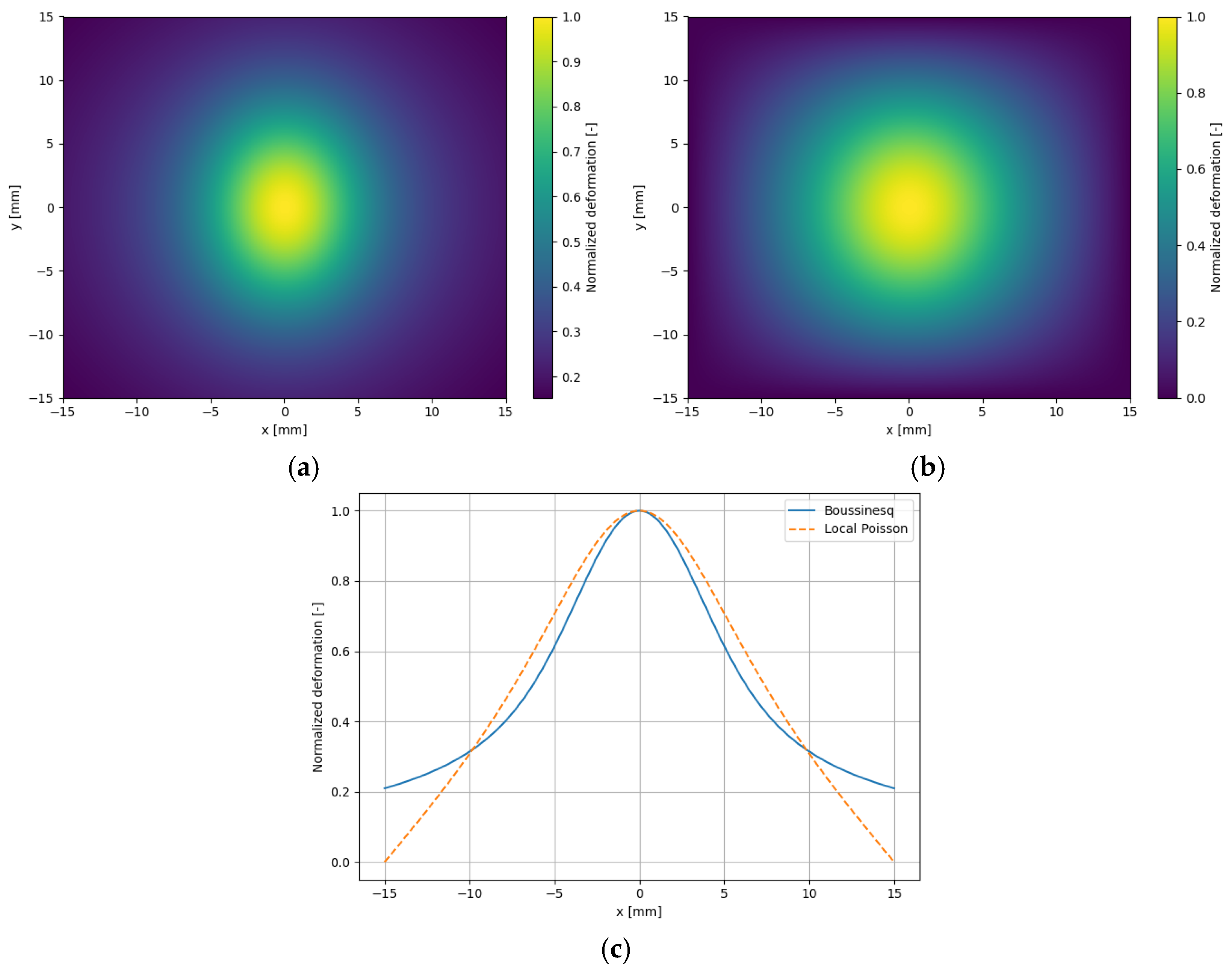
To provide a differential formulation compatible with automatic differentiation and to preserve the mesh-free nature of the PINN framework, a local Poisson-type equation (Equation (8)) is introduced as a local approximation of the elastic deformation field, motivated by the classical Boussinesq half-space solution. For the standalone dimensional formulation, a characteristic length (L) is required to provide the necessary dimensional scaling of the governing equation. However, the value of L is not known a priori. Consequently, the absolute deformation magnitude predicted by the local formulation cannot be uniquely validated against the Boussinesq solution. Instead, the accuracy of the proposed local operator was assessed by comparing the normalized spatial deformation field with the classical Boussinesq solution. The detailed validation procedure and results are provided in Appendix A.

$${{\nabla }^{2}u}_z(x,y)=-{\displaystyle \frac{2(1-{\nu }^2)}{E \left(L\right) }}p(x,y)$$

(8)

This reformulation, as presented in Equation (8), transforms the global integral representation problem into a local PDE, which can be efficiently enforced through AD within the PINNs. To enable AD of the deformation governing equation, the deformation field must be available within the computational graph. However, the elastic deformation is not introduced as an independent neural network output, but is instead computed indirectly from the predicted film thickness by subtracting the rigid geometric gap. The rigid gap is determined from the geometric configuration together with the film thickness predicted by the neural network; consequently, the elastic deformation is obtained implicitly from their relation rather than being introduced as a separate neural network output. In this way, the elastic response is fully embedded within the film thickness representation, allowing its spatial derivatives to be consistently evaluated using AD within the PINNs.

In addition, the GT contact model is incorporated to represent asperity contact under mixed-lubrication conditions and is imposed as a physical constraint within the framework. This constraint is particularly relevant under mixed-friction conditions, where both the hydrodynamic pressure and the asperity contact pressure contribute to balancing the applied bearing load. Neglecting the asperity contact pressure would violate the load-balancing constraint, leading to physically inconsistent predictions of the hydrodynamic pressure and the resulting film thickness. Unlike the Reynolds equation for hydrodynamics and the Poisson-type equation for deformation, which are explicitly incorporated into the loss function, the contact model is treated implicitly through a functional constraint imposed by the load-balance loss. Since the GT contact model is formulated analytically rather than as an additional governing PDE, it was incorporated directly into the PINN framework without requiring a separate loss term, additional network outputs, or dedicated weighting factors. Similar to the elastic deformation, the asperity contact pressure is calculated as an internal quantity and is not treated as an explicit network output, unlike the film thickness and hydrodynamic pressure. Introducing additional outputs and corresponding loss terms would increase the complexity of the optimisation problem, potentially reducing the prediction accuracy of the hydrodynamic pressure and film thickness. The formulation of the corresponding physics-based loss terms is presented in Section 2.2.3.

2.2.3. Loss Formulation

Building upon the data-driven and physics-informed components, seven custom loss functions based on the MSE are defined within the proposed framework. These loss terms quantify deviations from the available reference data as well as violations of the governing equations and physical constraints, thereby guiding the network optimisation during training. The first four loss terms correspond to the data-driven component, representing the supervised component of the model. In particular, Equations (9) and (10) define the losses ${\mathcal{l}}_p$ and ${\mathcal{l}}_h$, which measure the prediction errors associated with the hydrodynamic pressure and oil film thickness, weighted by C₁ and C₂, respectively. Here, N_T represents the total number of training points in the θ- and z-directions, with p_T and p_P the true and predicted pressure values, and h_T and h_P the true and predicted film thickness values.

$${\mathcal{l}}_p=C_1{\displaystyle \frac{1}{N_T}}{\sum }_{i=1}^{N_T}{\left(p_T\right({\theta }_i,z_i)-p_p({\theta }_i,z_i\left)\right)}^2$$

(9)

$${\mathcal{l}}_h=C_2{\displaystyle \frac{1}{{ N}_T}}{\sum }_{i=1}^{N_T}{\left(h_T\right({\theta }_i,z_i)-h_p({\theta }_i,z_i\left)\right)}^2$$

(10)

Besides the standard first two supervised loss terms, Equations (11) and (12) introduce two additional loss functions. These loss terms target the discrepancies in the maximum hydrodynamic pressure and the minimum oil film thickness across the computational domain. Their relative contributions are controlled by the weighting coefficients C3 and C4, respectively. In this formulation, N_D denotes the total number of domain points, which is 1944 in the present framework. Here, p_T,max and p_P,max are the true and predicted maximum pressure values, and h_T,min and h_P,min are the true and predicted minimum film thickness values, respectively. These constraints enforce the predicted global extrema of the pressure and film thickness fields to remain close to the reference values. Since the model does not always reproduce the exact global extrema or minimum values accurately, these additional constraints were introduced to improve the prediction accuracy of the maximum hydrodynamic pressure as well as the minimum film thickness.

$${\mathcal{l}}_{p,max}=C_3{\displaystyle \frac{N_D}{N_T}}{\sum }_{i=1}^{{\displaystyle \frac{N_T}{N_D}}}{\left(p_{T,max}\right({\theta }_i,z_i)-p_{p,max}({\theta }_i,z_i\left)\right)}^2$$

(11)

$${\mathcal{l}}_{h,min}=C_4{\displaystyle \frac{N_D}{{ N}_T}}{\sum }_{i=1}^{{\displaystyle \frac{N_T}{N_D}}}{\left(h_{T,min}\right({\theta }_i,z_i)-h_{p,min}({\theta }_i,z_i\left)\right)}^2$$

(12)

The physics-informed component is represented by the remaining three loss functions. The first physics-informed loss term captures the first PDE residual, which corresponds to the Reynolds equation by Patir and Cheng (see Equation (1)) and is defined in Equation (13). In Equation (13), C₅ denotes the weighting factor assigned to the PDE residual. The residual is evaluated at collocation points (N_C), which are distributed across the computational domain to enforce the governing physics during network training. A detailed description and discussion of the collocation point strategy is given in Section 2.2.4.

$${\mathcal{l}}_{\mathrm{R}\mathrm{e}\mathrm{y}\mathrm{n}\mathrm{o}\mathrm{l}\mathrm{d}\mathrm{s}}=C_5{\displaystyle \frac{1}{N_C}}{\sum }_{i=1}^{N_C}{(0-{(3h^2\left({\varphi }_{\theta }{\displaystyle \frac{dh}{d\theta }}·{\displaystyle \frac{dp}{d\theta }}+{\varphi }_z{\displaystyle \frac{dh}{dz}}·{\displaystyle \frac{dp}{dz}}\right)+h^3\left({\varphi }_{\theta }{\displaystyle \frac{d^{2}p}{d{\theta }^2}}+{\varphi }_z{\displaystyle \frac{d^{2}p}{d{z}^2}}\right)-6\eta u_1{\varphi }_s{\displaystyle \frac{dh}{d\theta }}-12\eta {\displaystyle \frac{dh}{dt}})}_i)}^2$$

(13)

The second physics-informed loss term, denoted as ${\mathcal{l}}_{Deformation}$, captures the PDE residual associated with the deformation of the bearing surface. Unlike the standalone dimensional formulation, the deformation equation is employed as a normalised physics-based residual. Consequently, the loss formulation does not require the introduction of an empirical effective characteristic length (L) whose value is not known a priori. Instead, the normalised form is used directly within the loss function. The corresponding deformation loss is incorporated into the framework as shown in Equation (14).

$${\mathcal{l}}_{\mathrm{D}\mathrm{e}\mathrm{f}\mathrm{o}\mathrm{r}\mathrm{m}\mathrm{a}\mathrm{t}\mathrm{i}\mathrm{o}\mathrm{n}}=C_6{\displaystyle \frac{1}{N_C}}{\sum }_{i=1}^{N_C}{(0-{\displaystyle \frac{d^{2}u}{d{\theta }^2}}+{\displaystyle \frac{d^{2}u}{d{z}^2}}-({\displaystyle \frac{2({\nu }^2-1)}{E}}p(\theta ,z){)}_i)}^2$$

(14)

Unlike the first two loss terms in the physics-informed component, which are formulated as local physics-based loss terms, the third physics-informed loss term represents the load balance equation and is formulated as a global physics-based constraint. Since the load balance equation does not operate locally, it requires that the integral of the pressure distribution over the entire domain equals the applied external load (see Equations (2) and (3)). Consequently, it depends on the cumulative contribution of all spatial points rather than on individual pointwise behaviour. For this reason, it is formulated as a global physics-based loss term, as shown in Equation (15). In this formulation, f_T represents the externally applied load, while f_ph+pa denotes the total load contribution resulting from both the hydrodynamic pressure and the asperity contact pressure.

$${\mathcal{l}}_{load balancing}=C_7{\displaystyle \frac{N_D}{N_C}}{\sum }_{i=1}^{{\displaystyle \frac{N_C}{N_D}}}{\left(f_T\right(x_i,y_i)-f_{p_h+p_a}(x_i,y_i\left)\right)}^2$$

(15)

2.2.4. Training Strategy

Based on the loss formulation described above, the training process aims to minimise the combined loss function by reducing the prediction errors, PDE residuals, and constraint violations. As PINN frameworks involve numerous hyperparameters that strongly influence model accuracy, their selection and tuning must be carried out systematically. Since no universal method exists for determining the optimal configuration, multiple experiments were performed with different setups to identify a configuration that yields good performance [42]. However, a comprehensive comparison of different network architectures and hyperparameter optimization strategies is beyond the scope of this study. The training strategy adopted for the proposed framework is organized into three subsections: Section Training, Validation, and Testing Simulation Cases, Section Loss Balancing and Optimization, and Section Model Validity Domain and Reproducibility.

Training, Validation and Testing Simulation Cases

The training strategy for the proposed PINN framework starts with defining the number of training and collocation data points, which are both utilized during the training process. Firstly, the training points (N_T) represent the input and corresponding true output obtained from the EHD simulations, as presented in Section 2.1.1. These points provide the ground-truth data for the supervised component of the framework. In contrast to the training points (N_T), which are associated with known input–output pairs, the collocation points (N_C) do not have corresponding target outputs. Rather, these are specific points within the training domain that are used to enforce the governing physical equations via the physics-informed component of the framework, representing the unsupervised part of the PINN.

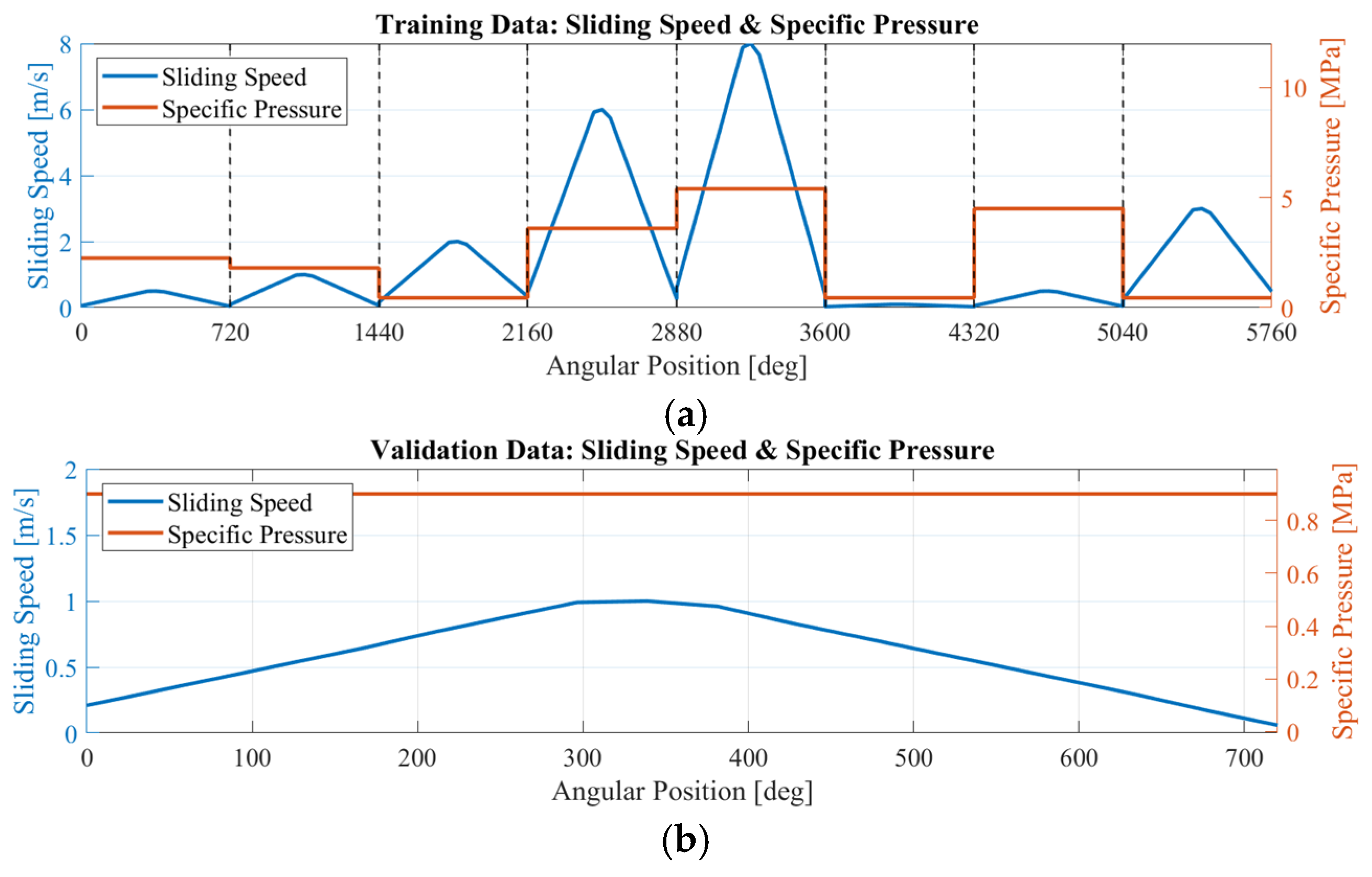
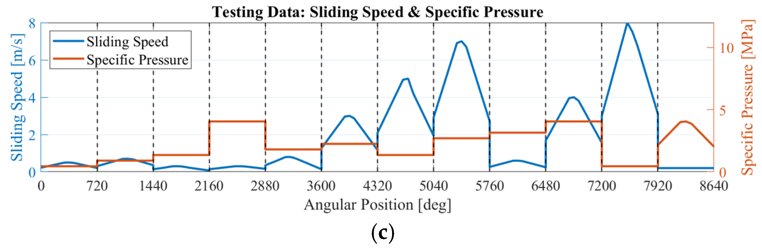
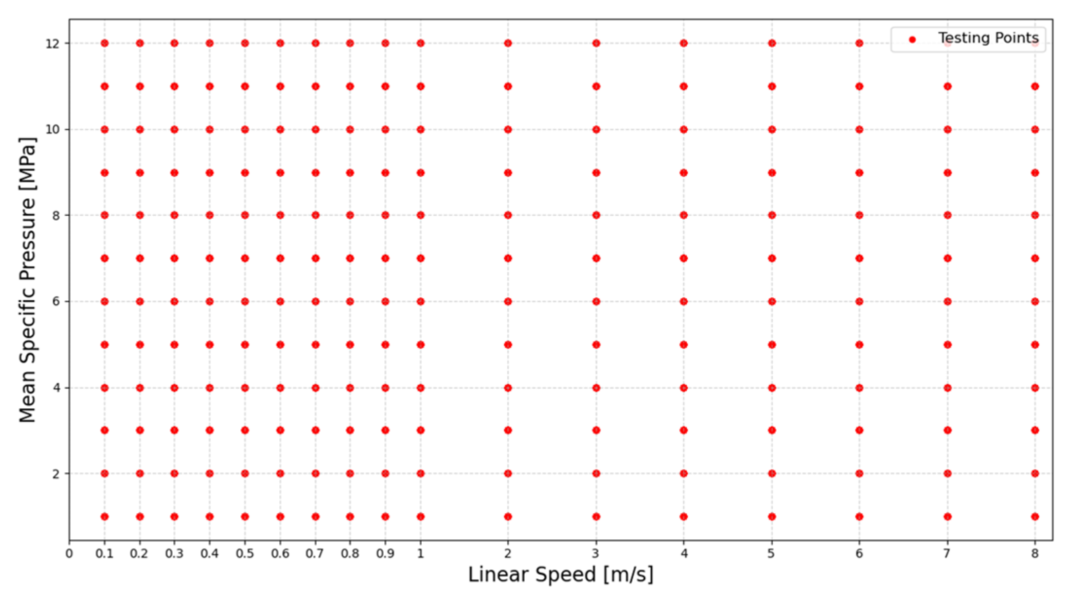
As the proposed real-time model is primarily intended for dynamic loading applications, only data obtained from dynamic simulations were used as training points for the supervised training process. The supervised training process utilizes only two randomly selected discrete time steps from each of eight dynamic simulations (see Figure 3), where every time step represents a specific operating condition in terms of speed, load, and temporal sequence during the system evolution. The random selection was performed under the condition that the selected training points represent at least two out of the three varying operating parameters, namely rotational speed, specific pressure, and time sequence. Consequently, the training set consists of 16 randomly chosen time steps. Due to the significantly increased memory requirements and computational cost associated with large independently sampled collocation datasets, the input data from the same eight simulations are additionally employed as collocation points, thereby avoiding the need for a separate collocation sampling process. However, only the selected discrete time steps are used as supervised training points, while the remaining input data are utilized exclusively for enforcing the physics-based constraints. For validation during the training process, one independent dynamic simulation case was used (see Figure 3b). The remaining 12 dynamic cases (see Figure 3c), together with all 204 static cases (see Figure 4), were reserved exclusively for testing. Neither the validation case nor the test cases were included in the training dataset.

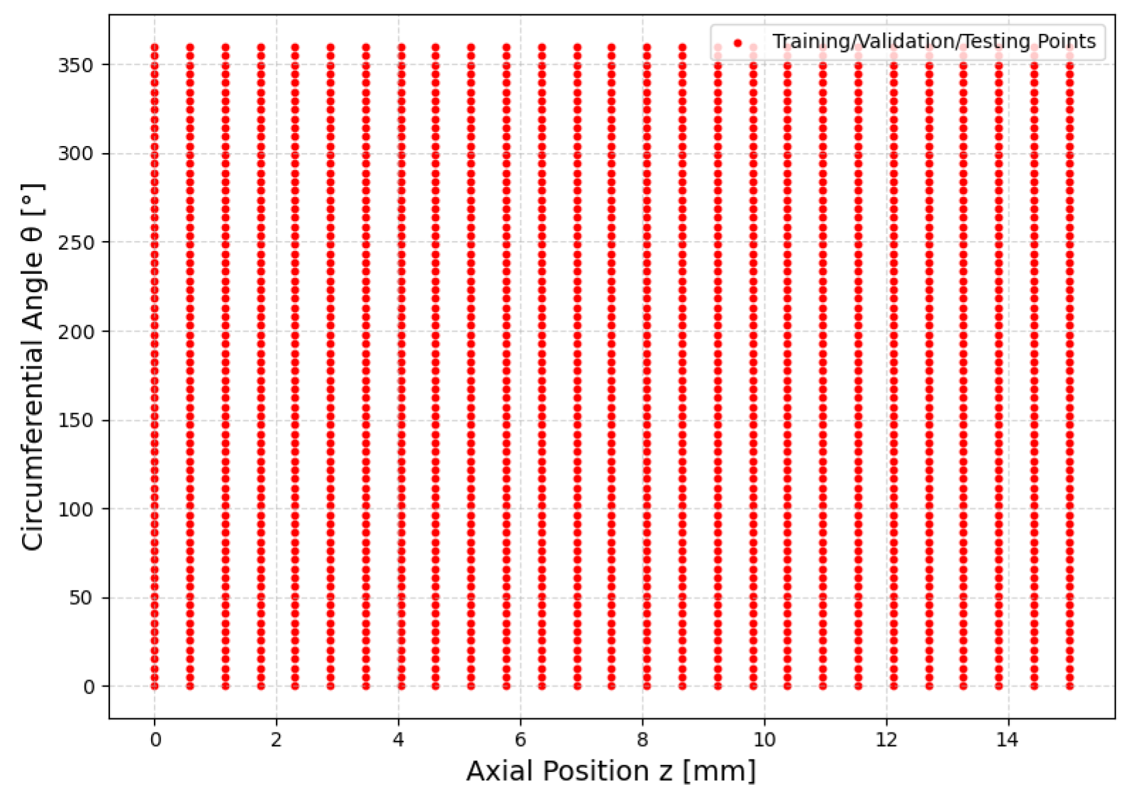
The pressure and film thickness distributions are evaluated at 1944 spatial locations distributed throughout the bearing domain in the circumferential (θ) and axial (z) directions, as shown in Figure 5. Although random points could also be used within the meshless PINN framework, the discretized EHD point distribution was retained in this work to satisfy the load-balancing constraint, which requires the integration of the pressure distribution to determine the resulting force. Nevertheless, the proposed PINN remains meshless, since the governing equations are evaluated at discrete points rather than solved on a connected computational mesh.

Loss Balancing and Optimization

Prior to training, all network weights and biases are initialized using the Kaiming uniform (He) initialization to provide initial values for the optimization process. These initial values serve as the starting point for the subsequent optimization process. The trainable parameters are subsequently optimized using the Adam algorithm with a dynamic learning rate starting at η = 10⁻³. While the Adam optimizer adaptively scales parameter updates, a learning rate scheduler is additionally employed to adjust the global learning rate during training, improving convergence and stability. A major challenge during training PINN frameworks is the effective balancing of the multiple loss terms involved. In this framework, the self-adaptive loss balancing method proposed by Xiang [68] is employed to automatically determine the relative importance of each loss term, eliminating the need for manual weighting. An independent adaptive weighting coefficient is assigned to each of the seven loss terms. These coefficients are initialized equally and updated automatically during training based on the relative convergence of the individual loss terms. Consequently, the relative contribution of each loss term is continuously adjusted throughout the optimization, eliminating the need for manually prescribed weighting coefficients.

Model Validity Domain and Reproducibility

The validity domain of the proposed PINN is defined by the input parameter ranges corresponding to the operating conditions of the experimental test rig. The investigated operating conditions cover sliding speeds ranging from 0.1 to 8 m/s and radial loads from 0.45 to 5.45 kN, corresponding to mean specific pressures between 1 and 12 MPa. Within these bounds, the network is intended for interpolation. Predictions outside this parameter space require extrapolation. Although a limited number of validation and testing cases extend beyond the training range, the extrapolation capability of the proposed PINN has not been systematically evaluated in the present study.

To facilitate the reproduction of the proposed framework and the reported results, the network architecture, training hyperparameters, and Training settings are summarized in

Table 3. Framework configuration and training parameters.

Bearing Geometry	Diameter (D)	30 mm
	Width (B)	15 mm
	Radial clearance	25 μm
Coordinate system	Circumferential coordinate	θ ∈ [0, πD]
	Axial coordinate	z ∈ [0, B]
Computational domain	Circumferential sampling points (θ)	72
	Axial sampling points (z)	27
Neural network	Input variables	z, θ, t, F, n
	Output variables	P, h
	Hidden layers	4
	Neurons/layer	256
	Dropout rate	0.1
	Activation functions	Tanh, Sigmoid, Softplus
Training settings	Training domains (time steps)	16
	Total training data points	31,104
	Collocation domains (time steps)	128
	Total Collocation data points	248,832
	Optimizer	Adam
	Initial learning rate	10−3
	Weight decay (network parameters)	10−5
	Learning-rate scheduler	StepLR, 5000 epochs, 0.9
	Convergence criterion	Early stopping (patience = 5000 epochs)

. In addition, a summary of the main PINN training workflow is provided in the Supplementary Materials.

3. Results and Discussion

The predictive performance of the trained PINN model is assessed and discussed in this section. It is divided into two subsections. Section 3.1 comprises three parts: training behavior and loss evolution, prediction accuracy of the film thickness and hydrodynamic pressure, and identification of the onset of mixed lubrication. Section 3.2 presents the post-training evaluation and is divided into two parts. The first part assesses the model’s generalization capability under static operating conditions, while the second part evaluates its performance under dynamic operating conditions. The trained model is validated and tested using numerical EHD simulation data introduced in Section 2.1.

3.1. Model Behaviour and Validation Throughout Training

3.1.1. Training Convergence Analysis

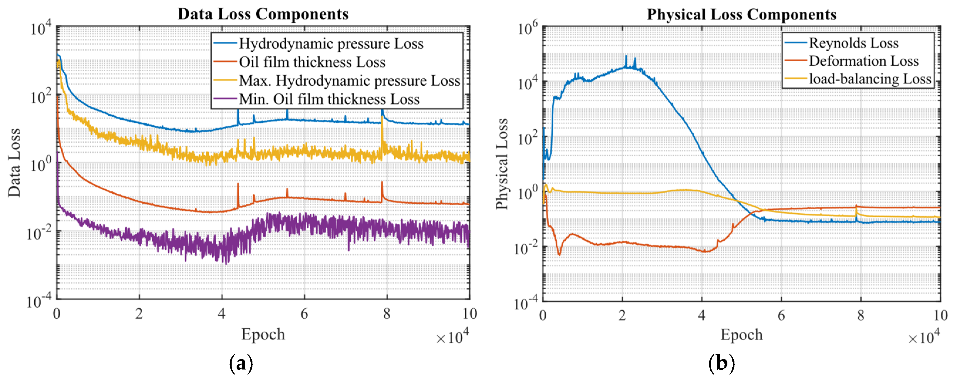
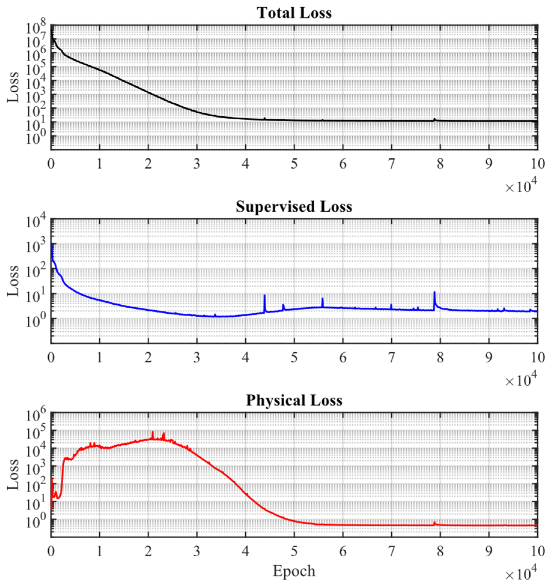
The loss history reflects the convergence of the optimization process, demonstrating how the network progressively satisfies both the supervised data and the governing physical equations while improving its predictive performance on the validation dataset. Stable convergence of the model is achieved after approximately 60,000 training epochs. Beyond this point, the prediction accuracy improves only gradually until around 90,000 epochs, after which the model performance remains nearly constant. The convergence behavior of the total, supervised, and physics-based losses is depicted in Figure 6, whereas Figure 7 presents the evolution of the corresponding individual loss components. The evolution of the total, supervised, and physical losses during training reveals a three-stage learning process. At the beginning of training, the supervised (data) loss decreases rapidly, indicating that the model quickly fits the available data. In this phase, the total loss is primarily dominated by the supervised term, where the pressure loss components dominate, while the film thickness loss components contribute secondarily, as shown in Figure 7a. In contrast to the supervised loss, the physical loss shows transient behavior followed by a rapid increase, indicating that satisfying the governing physical equations is more challenging in the initial phase. As training progresses, dynamic loss weighting decreases the weight of the data loss while increasing the weight of the physical loss. This shift in optimization focus from data dominance toward physics dominance is followed by a significant drop in the physical loss in the later stages, indicating that the model begins to better satisfy the underlying physical constraints. In this stage, the Reynolds equation loss dominates the later stage of training, while the deformation and load-balancing losses contribute as secondary terms, as shown in Figure 7b. In the later stages of training, a pronounced decrease in the physical loss is observed, indicating improved satisfaction of the governing physical constraints. Overall, the observed training history indicates a progressive transition from data-driven learning to physics-informed refinement, reflecting the dynamic rebalancing of the individual loss contributions during optimisation. In the later stages, the model converges toward a balanced compromise between accurately fitting the data and satisfying the governing physical laws.

3.1.2. Validation of Hydrodynamic Pressure and Film Thickness Predictions

Model performance was assessed by comparing the PINN predictions with the numerical EHD reference solution. The evaluation employed the coefficient of determination (R² score) and the Root Mean Square Error (RMSE) were used. In addition, the relative errors of the maximum hydrodynamic pressure and the minimum oil film thickness were calculated to quantify deviations from the reference solution. The error for the peak hydrodynamic pressure was calculated relative to the maximum peak pressure observed in the entire available dataset (23.363 MPa), while the percentage error for the film thickness was determined with respect to the radial clearance (25 μm). After the training process, the validation results for both the pressure and film thickness distributions achieved R² scores of 0.9553 and 0.9956, respectively. These values correspond to the validation load case consisting of 18 time steps (see Figure 3b).

Table 4. Results of the model validation.

Time Step	Liner Speed [m/s]	Specific Pressure [MPa]	Hydrodynamic Pressure					Oil Film Thickness
			R2 [-]	RMSE [MPa]	Peak True [MPa]	Peak Predicted [MPa]	Abs. Error [%]	R2 [-]	RMSE [μm]	Min. True [μm]	Min. Predicted [μm]	Abs. Error [%]
1	0.21	0.9	0.9504	0.2189	5.292	6.090	3.42%	0.9965	1.1576	1.673	1.440	1.00%
2	0.32	0.9	0.9536	0.2379	5.942	6.588	2.77%	0.9974	0.9970	1.684	1.543	0.60%
3	0.43	0.9	0.9759	0.1976	6.718	6.925	0.89%	0.9981	0.8307	1.737	1.646	0.39%
4	0.54	0.9	0.9753	0.2222	7.319	7.305	0.06%	0.9987	0.6848	1.834	1.736	0.42%
5	0.65	0.9	0.9659	0.2792	7.814	7.548	1.14%	0.9989	0.6245	1.985	1.828	0.67%
6	0.77	0.9	0.9624	0.3004	8.006	7.769	1.01%	0.9987	0.6708	2.146	1.928	0.93%
7	0.88	0.9	0.9561	0.3231	7.910	7.799	0.48%	0.9980	0.8012	2.395	1.997	1.70%
8	0.99	0.9	0.9488	0.3453	7.732	7.909	0.76%	0.9970	0.9752	2.660	2.075	2.50%
9	1.00	0.9	0.9412	0.3637	7.496	7.816	1.37%	0.9946	1.2869	2.931	2.042	3.81%
10	0.96	0.9	0.9422	0.3454	6.862	6.180	2.92%	0.9936	1.3550	3.874	3.142	3.13%
11	0.84	0.9	0.9629	0.2771	6.853	6.573	1.20%	0.9948	1.2239	3.856	3.592	1.13%
12	0.73	0.9	0.9716	0.2431	6.865	6.825	0.17%	0.9948	1.2247	3.778	3.871	0.40%
13	0.62	0.9	0.9737	0.2355	6.939	6.990	0.22%	0.9945	1.2798	3.643	3.918	1.18%
14	0.51	0.9	0.9714	0.2482	7.075	7.106	0.13%	0.9941	1.3446	3.453	3.792	1.45%
15	0.40	0.9	0.9631	0.2859	7.252	7.112	0.60%	0.9938	1.4064	3.187	3.554	1.57%
16	0.29	0.9	0.9468	0.3493	7.481	7.053	1.83%	0.9934	1.4744	2.861	3.210	1.49%
17	0.17	0.9	0.9190	0.4422	7.766	6.950	3.49%	0.9929	1.5719	2.453	2.843	1.67%
18	0.06	0.9	0.9143	0.4384	7.802	6.749	4.51%	0.9913	1.8033	1.955	2.441	2.08%

summarizes R² scores, RMSE values, and the corresponding reference and predicted results. It also reports the errors associated with the maximum hydrodynamic pressure and the minimum oil film thickness.

Overall, the validation results demonstrate good agreement between the predicted and reference solutions for all investigated operating conditions. According to Table 4, no consistent correlation was observed between the operating conditions and the prediction accuracy of either the hydrodynamic pressure or the film thickness. In the case of the hydrodynamic pressure R² values ranged from 0.9143 to 0.9759, indicating generally good agreement with the true values. Although some time steps exhibited comparatively lower R² values for hydrodynamic pressure, the corresponding absolute errors and RMSE values remained low, with average values of 1.5% and 0.3 MPa, respectively. These lower R² values for hydrodynamic pressure are mainly attributed to the relatively small variation range of the pressure distribution in these cases, which makes the R² metric more sensitive to minor local differences between the predicted and reference values. In the case of the film thickness, all predicted values exhibited consistently high accuracy, with R² values remaining values vary between 0.9913 and 0.9989 and showing very good agreement with the reference values. Furthermore, the corresponding absolute errors and RMSE values remained low, with average values of 1.45% and 1.1 μm, respectively.

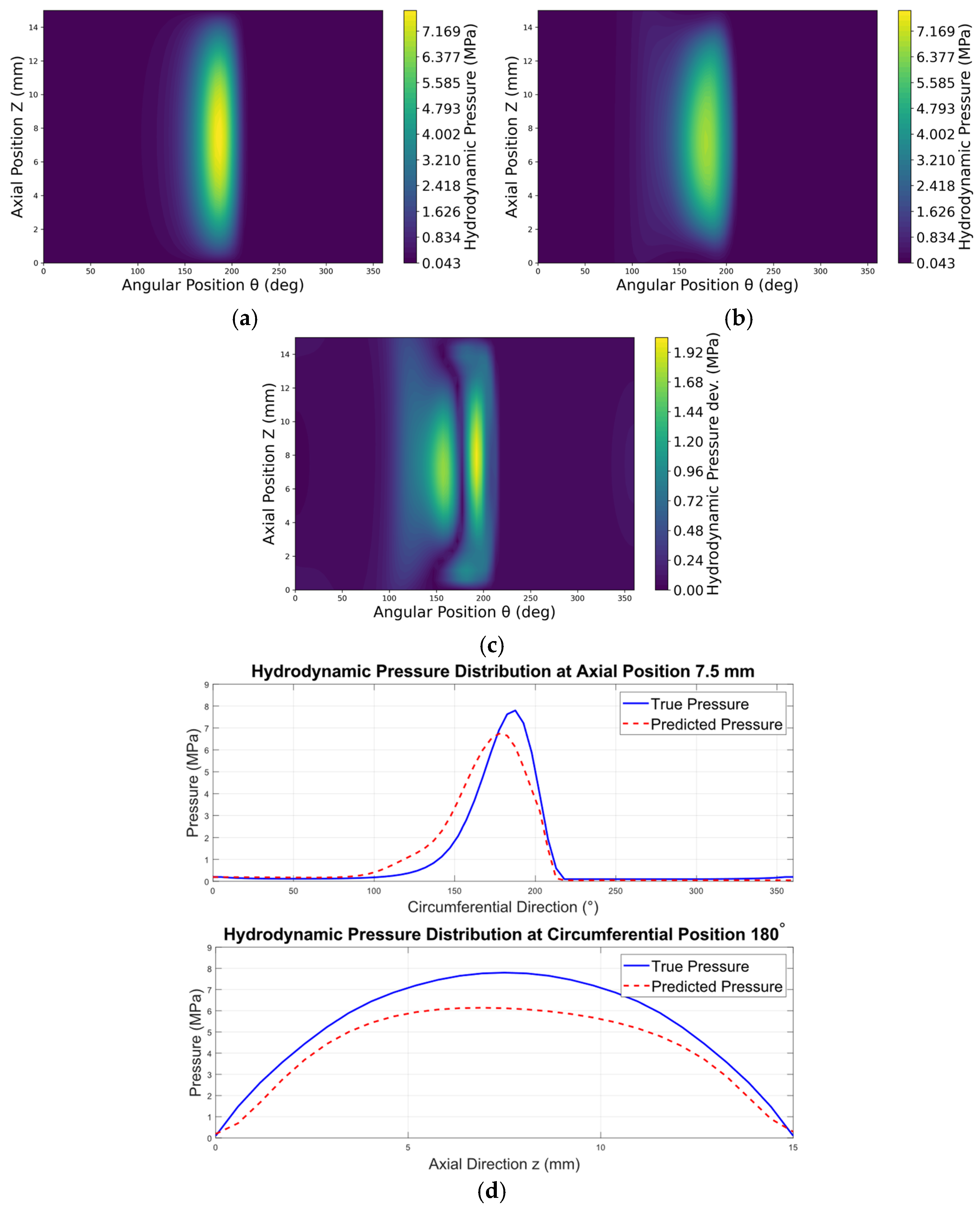
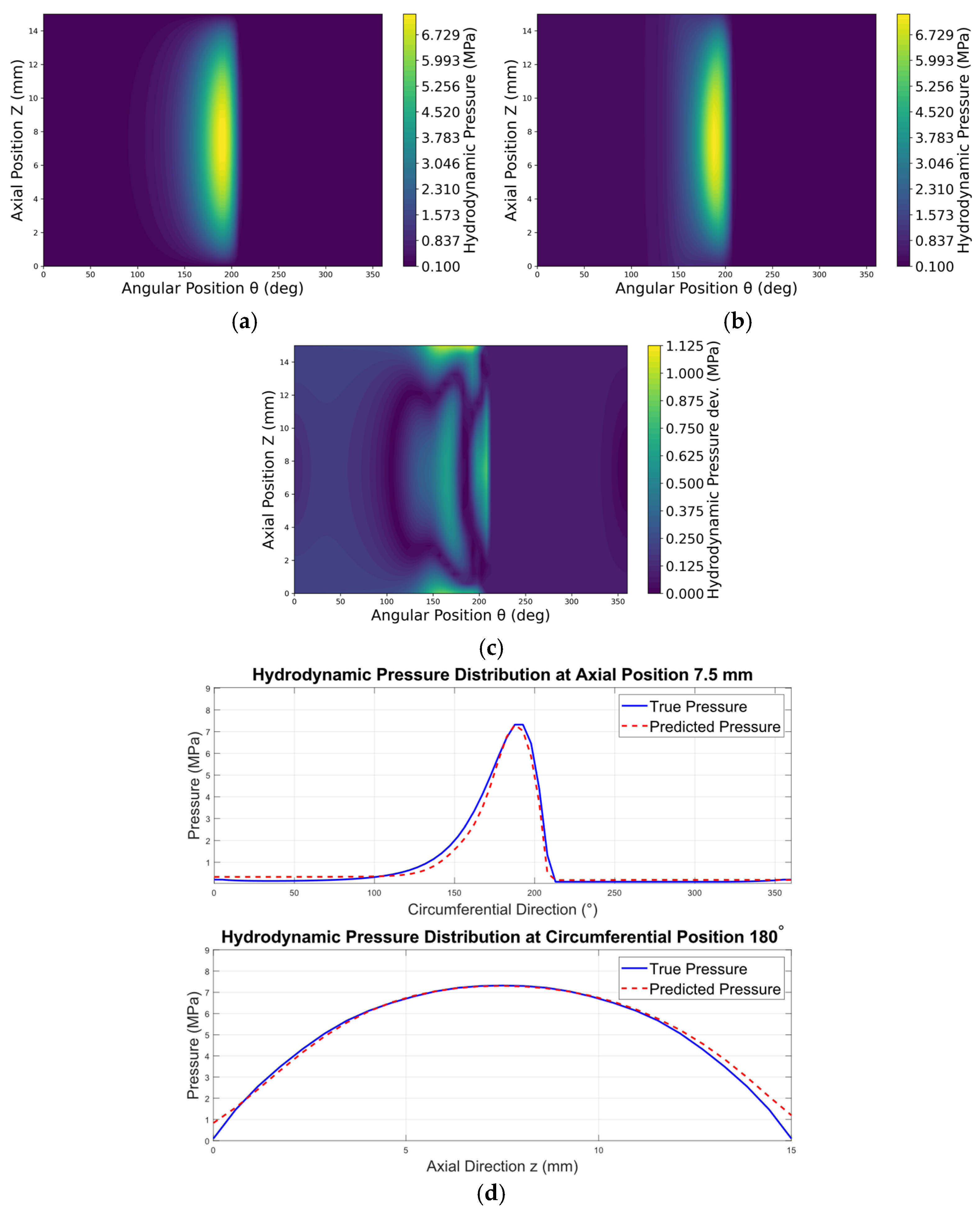
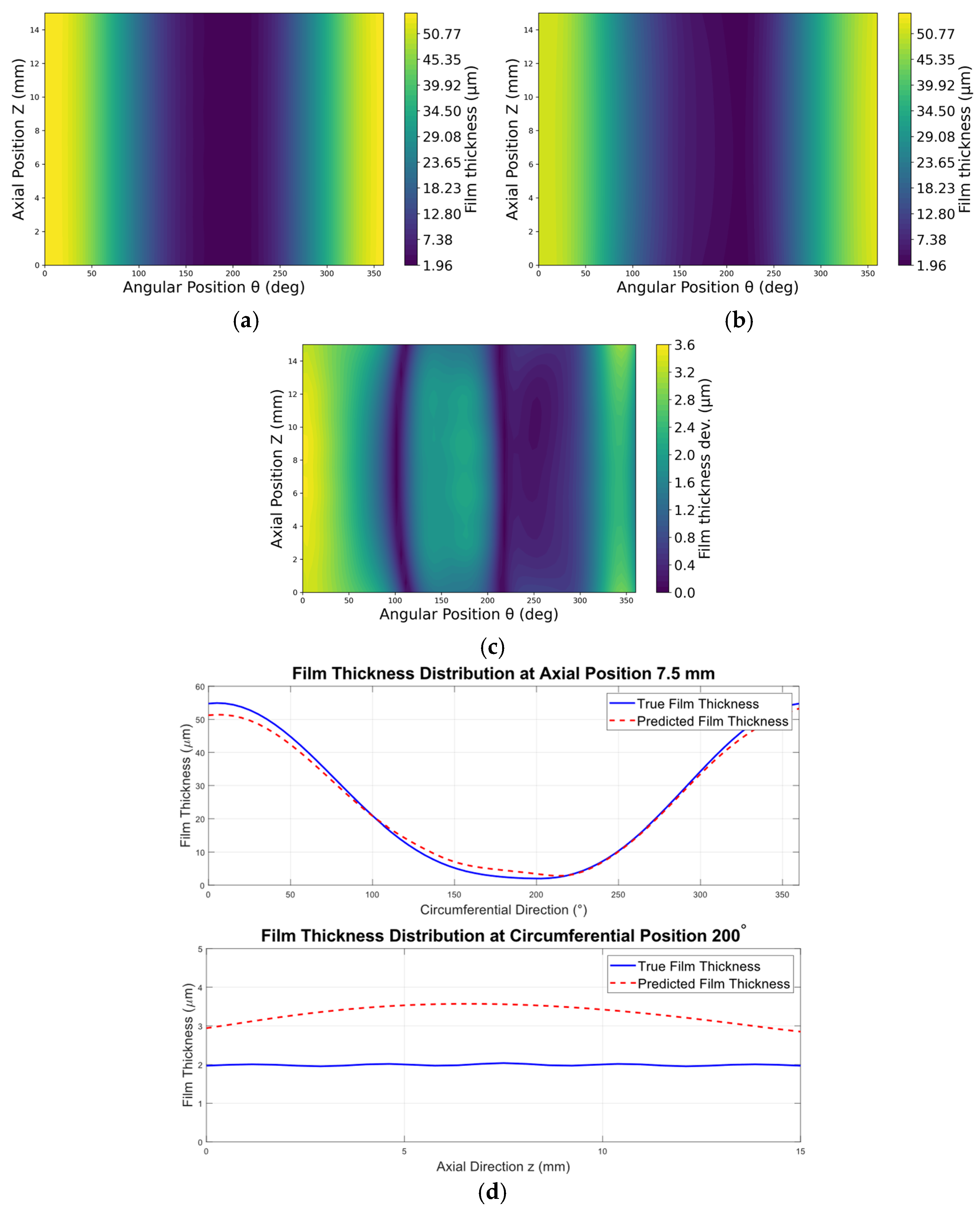
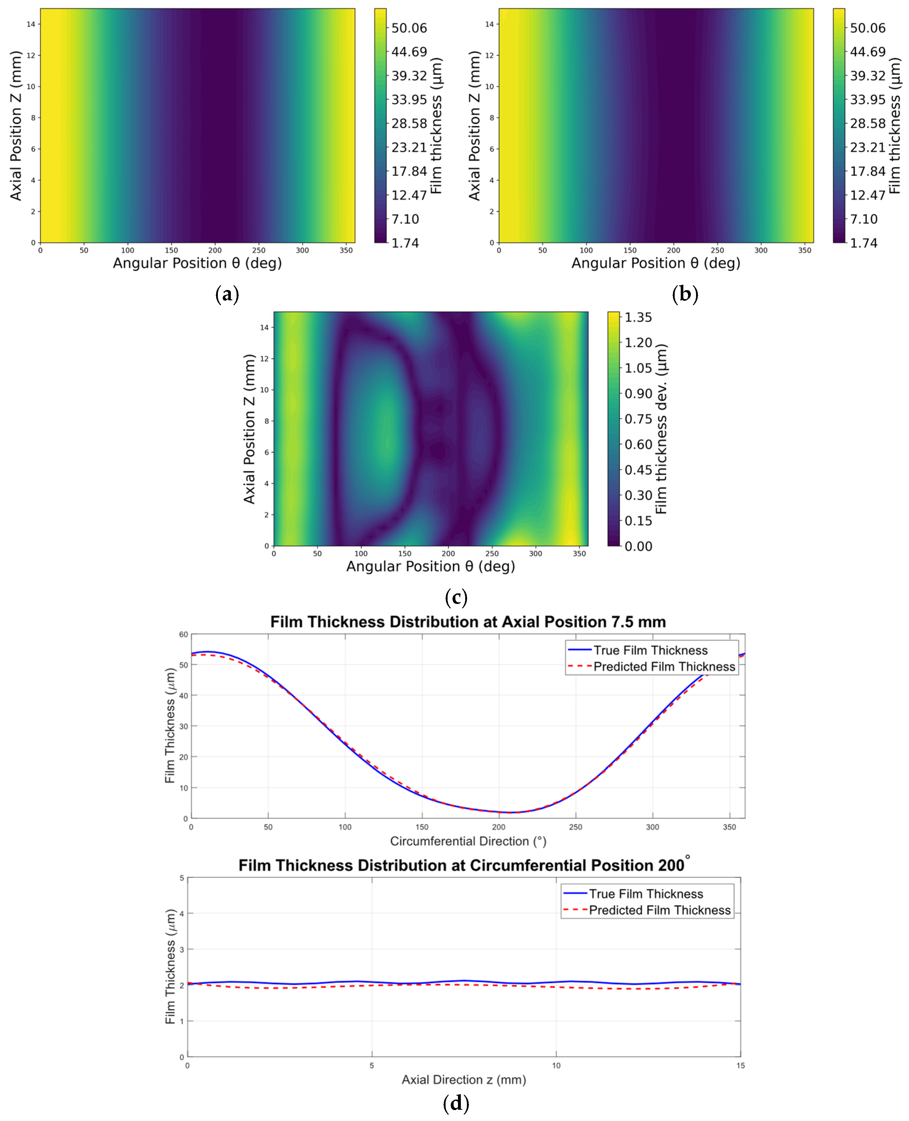
To further evaluate the predictive performance of the proposed model, two representative time steps were selected for detailed comparison: one case with comparatively lower prediction accuracy and another with higher prediction accuracy. The corresponding 2D distributions of the hydrodynamic pressure and film thickness for both the true and predicted solutions are presented in Figure 8, Figure 9, Figure 10 and Figure 11. Figure 8 and Figure 9 correspond to the 18th time step, which exhibits comparatively lower prediction accuracy (see Table 4), with R² values of 0.9143 for the hydrodynamic pressure and 0.9913 for the film thickness. The lower prediction accuracy observed at the 18th time step can be attributed to the very low sliding speed of 0.06 m/s, which was not represented in the training or collocation datasets. Consequently, the PINN model was required to extrapolate beyond the trained operating range, resulting in reduced prediction accuracy. In contrast, Figure 10 and Figure 11 correspond to the 4th time step, which shows comparatively higher prediction accuracy (see Table 4), with R² values of 0.9753 for the pressure and 0.9987 for the film thickness. Although the two selected time steps represent low- and high-accuracy cases, the predicted hydrodynamic pressure and film thickness distributions closely match the corresponding EHD reference distributions in both the axial (z) and circumferential (θ) directions.

For both time steps, the spatial distribution of the pressure prediction error remains nearly identical, with only minor differences in magnitude (see Figure 8c and Figure 10c). In contrast, the spatial distribution of the film thickness prediction error differs slightly between the two time steps, although the overall patterns remain similar (see Figure 9 and Figure 11). For the 18th time step (0.06 m/s), the peak film thickness errors are mainly located near circumferential angles of 45° and 150°. In contrast, for the 4th time step (0.54 m/s), they are located near 45° and 330°. This shift in error locations can be explained by changes in the magnitude and distribution of hydrodynamic pressure prediction errors across different operating conditions, particularly at very low sliding speeds outside the trained parameter range. These pressure deviations consequently lead to deviations in the calculated elastic deformation, which in turn affect the predicted film thickness. As illustrated in Figure 8d and Figure 9d, the maximum film thickness deviations occur in the same regions where the largest pressure deviations are observed. Furthermore, the evaluated operating condition (0.06 m/s) lies outside the training velocity range (0.1–8 m/s), representing an unseen operating condition for the PINN.

3.1.3. Validation of Lubrication-Regime Identification

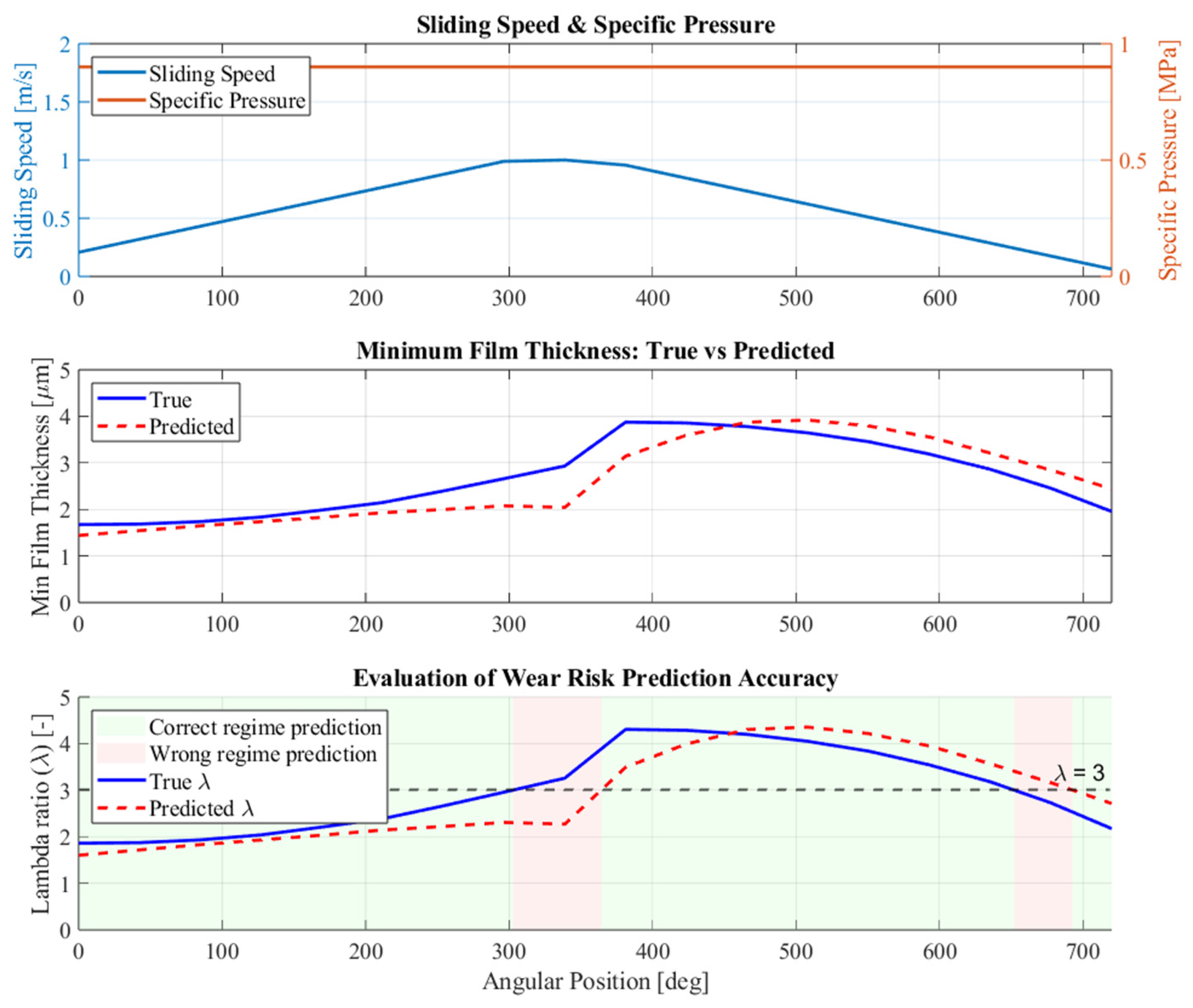
This subsection evaluates the proposed PINN framework’s ability to identify the lubrication regime correctly. As mentioned previously, the GT contact model and the resulting asperity contact pressure are incorporated into the physical component without being treated as explicit network outputs, unlike the film thickness and hydrodynamic pressure. Thus, the lambda ratio (λ) derived from the predicted film thickness is used to determine the onset of mixed-lubrication conditions [69]. A value of (λ = 3) is used as the threshold between hydrodynamic lubrication and mixed lubrication [69]. The results are summarised in Figure 12, which is divided into three subfigures. The first subfigure presents the operating conditions, namely the sliding speed and specific pressure, which were used as input parameters for the real-time model. The second subfigure compares the true and predicted minimum film thickness, which serves as the basis for the lubrication-regime assessment. The third subfigure presents the comparison between the lambda ratio (λ) and the corresponding lubrication-regime assessment based on the critical threshold of λ = 3. Regions highlighted in green indicate correct prediction of the lubrication regime, whereas red regions represent incorrect regime classification. Overall, the predicted λ closely matches the true λ; however, deviations are mainly observed near the transition regions around the critical threshold. These deviations are primarily attributed to a slight temporal delay of approximately 10 ms in the predicted λ evolution, which leads to deviations during the transition between the hydrodynamic and mixed-friction lubrication regimes. This deviation may be attributed to the limited temporal resolution of the employed datasets, as the transient simulation was represented by only 18 time steps over two shaft revolutions (720°). A finer temporal discretisation was not feasible due to hardware memory limitations and the increased computational effort associated with PINN training. Consequently, the network tends to interpolate between neighbouring temporal states, which can result in a slight temporal lag in the predicted response.

In terms of real-time computational performance, the proposed approach achieved an average computation time of approximately 3.4 ms per time step and 61.2 ms per load case, while the corresponding real operating time for two shaft revolutions was approximately 304 ms. In contrast, the equivalent conventional EHD simulation required approximately 35 h for the same operating condition. This demonstrates the strong potential of the proposed model for real-time assessment of lubrication regimes. The real-time model evaluation was performed on a laptop equipped with an AMD Ryzen 7 PRO 5850U processor (8 cores, 16 logical processors) and 32 GB RAM.

3.2. Generalisation Performance Evaluation

In this section, the proposed real-time model is evaluated under static and dynamic loading conditions to assess its ability to generalise across the test rig’s operating range. The testing data used for this evaluation are described in Section Training, Validation and Testing Simulation Cases. Since the film thickness determines the lubrication regime, the evaluation focuses on predicting film thickness and the corresponding transition between lubrication regimes.

3.2.1. Evaluation Under Dynamic Operating Conditions

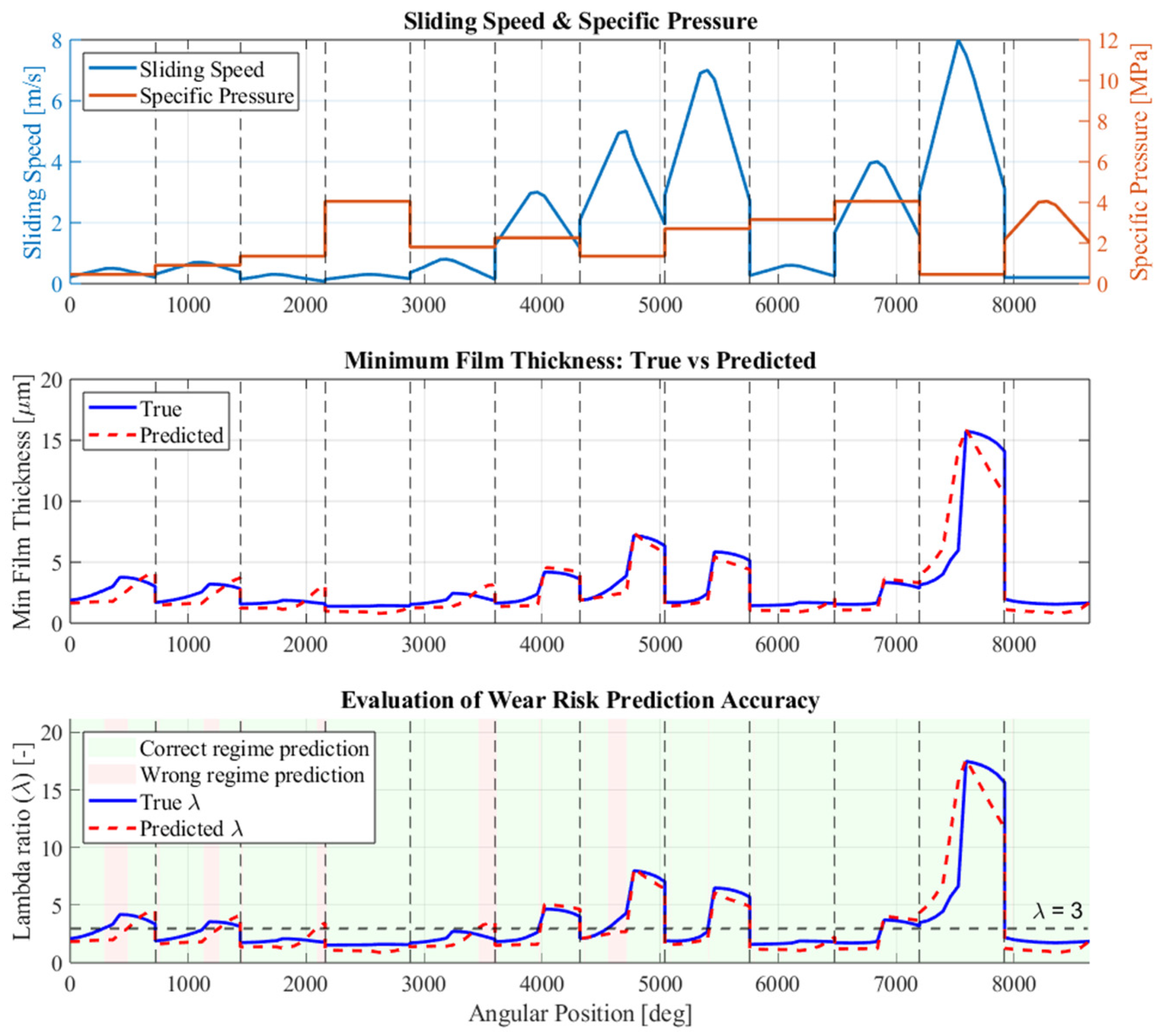
To evaluate the model under dynamic loading conditions, 12 dynamic load cases were considered. Although each load case was simulated separately, the corresponding operating conditions were sequentially supplied to the real-time model, with the time-step sequence restarting for each new load case. The corresponding results are summarised in Figure 13, which, similar to Figure 12, is divided into three subfigures. The first subfigure presents the operating conditions used as input to the real-time model, while the second and third subfigures show the corresponding film-thickness predictions and lubrication-regime assessment results based on the lambda ratio λ, respectively.

The results presented in Figure 13 show that the predicted λ closely follows the reference values, consistent with the validation cases. The mean model error for film-thickness prediction across the 12 dynamic load cases is 2.3%, while the corresponding error for lubrication-regime classification is 8.2%. The main deviations are observed near the transition regions around the critical threshold λ = 3, where small discrepancies in the predicted film thickness can lead to changes in the identified lubrication regime. Furthermore, it can be observed that the film thickness prediction error tends to increase with increasing magnitude of the true and predicted film thickness values. This behaviour indicates that larger absolute film thicknesses are associated with larger absolute deviations, although the proposed model accurately captures the overall trend and temporal evolution of the lubrication behaviour. Furthermore, the proposed real-time model tends to predict slightly lower film thicknesses in most cases, resulting in a conservative assessment of the lubrication regime compared to the high-fidelity model.

3.2.2. Evaluation Under Static Operating Conditions

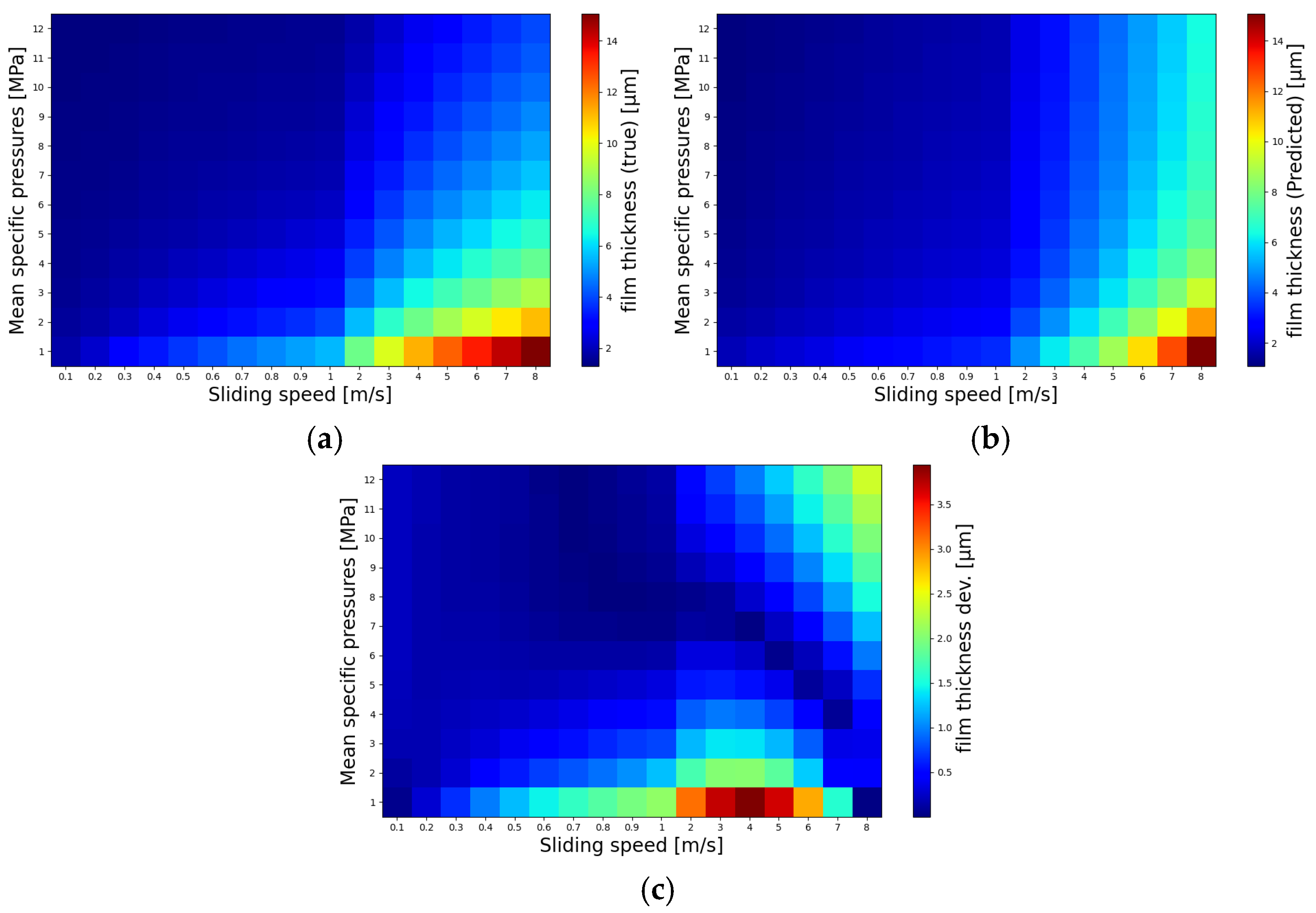
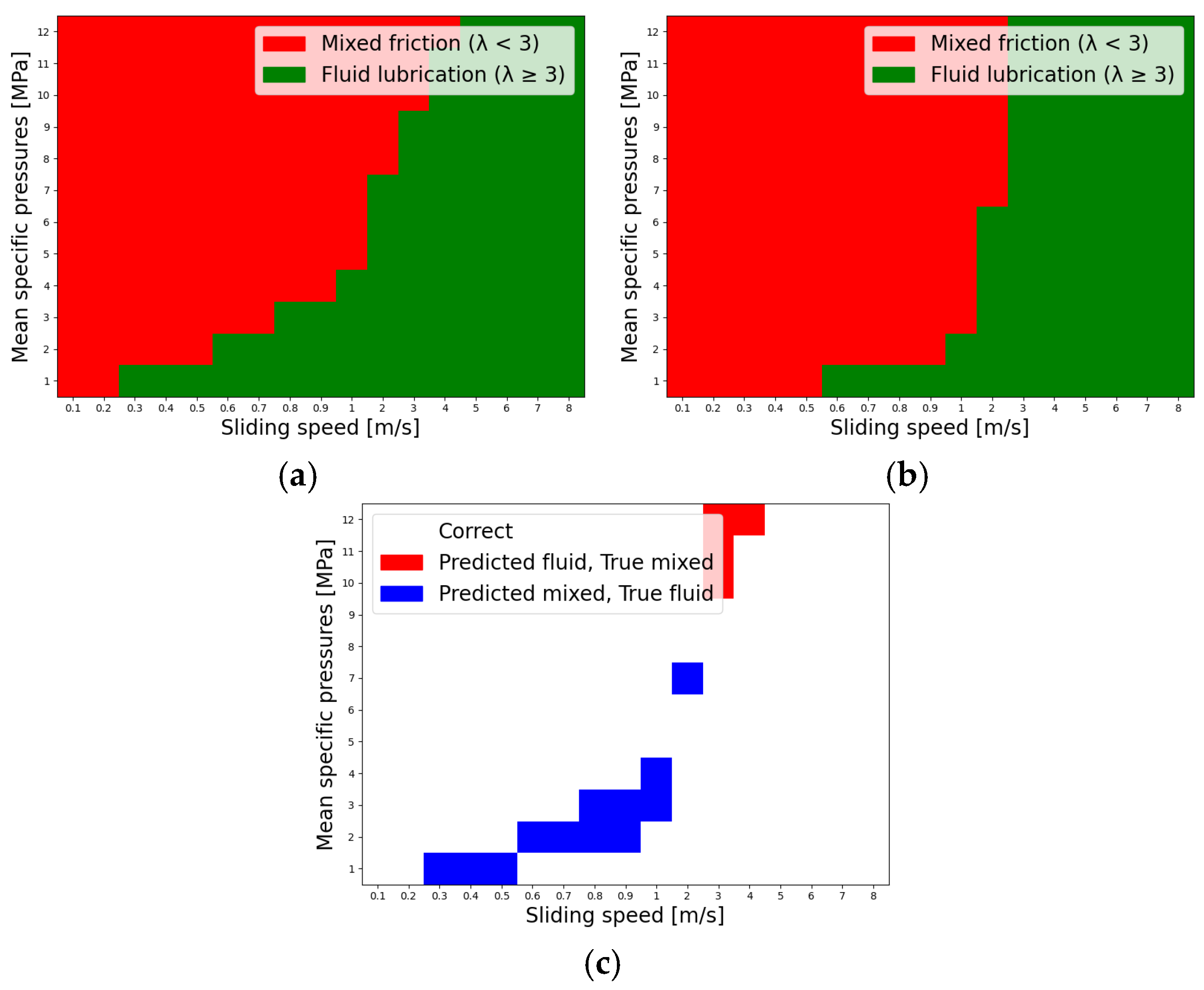
For the evaluation of the model under static loading conditions, 204 static load cases were considered, covering the operating range of the 30 mm sliding bearing test rig with sliding speeds from 0.1 to 8 m/s and specific pressures from 1 to 12 MPa. To apply the proposed model under static-loading operating conditions, the time-step input parameter was kept constant at t = 1 for all cases. The results are summarised in Figure 14 and Figure 15. Figure 14 presents the magnitudes of the true and predicted film thicknesses, together with their deviations, across the entire operating range. Figure 15 illustrates the corresponding lubrication regime classification based on the true and predicted film-thickness values, using the critical threshold λ = 3. In addition, the figure presents the associated prediction errors, indicating whether the film thickness is overestimated or underestimated. Although the proposed model was primarily trained on dynamic loading conditions, the results demonstrate that it can also accurately predict the lubrication behaviour under static operating conditions. The mean model error for film-thickness prediction across the 204 cases is 2.34%, while the corresponding error for the lubrication-regime classification is 7.8%. This is consistent with the results observed under dynamic operating conditions. The model exhibits similar behaviour under static loading conditions to that observed under dynamic loading. In particular, the film thickness prediction error tends to increase with increasing magnitude of the true film thickness values, as shown in Figure 14. This behaviour is more pronounced under static loading conditions, where the hydrodynamic lubrication regime dominates over a wider range of sliding speeds. Furthermore, the model exhibits the largest deviations under the lowest load condition, corresponding to a specific pressure of 1 MPa, over almost the entire sliding speed range. A similar behaviour was also observed for the corresponding load range under dynamic loading conditions in dynamic case 11 (see Figure 13), where comparable deviations between the true and predicted film thicknesses were observed, reaching a maximum of approximately 3.5 μm. The larger deviations observed at the lowest load condition are likely related to the strongly hydrodynamic operating regime in this load range. Under these conditions, the pressure gradients become comparatively small, with maximum hydrodynamic pressures ranging from approximately 2 to 4 MPa, while the film thickness increases significantly, making the film thickness more sensitive to small deviations in the predicted hydrodynamic pressure field. Without considering the lowest load condition corresponding to a specific pressure of 1 MPa, the maximum deviation between the true and predicted film thickness values was approximately 1.5 μm under dynamic loading conditions and 2 μm under static loading conditions. In both cases, the maximum deviations occurred at film thickness values greater than 5 μm, which still correspond to hydrodynamic lubrication conditions. Therefore, these deviations have only a minor influence on the overall assessment of the lubrication regime.

4. Conclusions

This work proposes a method that replaces computationally intensive EHD simulations with a PINN-based surrogate model while maintaining comparable accuracy. The proposed PINN-based model enables real-time lubrication-regime monitoring in sliding bearings, making it suitable for online condition monitoring. Using only the bearing load and shaft rotational speed as inputs, the model directly predicts the hydrodynamic pressure and lubricant film thickness. The predictions are guided by the key governing physics of the reference EHD formulation, including the transient Reynolds equation, the Greenwood–Tripp contact model, and bearing surface deformation. The predicted film thickness is subsequently used to calculate the lambda ratio (λ), which is then employed to identify the lubrication regime. The proposed model is developed and evaluated using a validated EHD model of a 30 mm sliding-bearing test rig, with the EHD simulation results serving as the reference data for training, validation, and testing. The main findings of this work are summarized as follows:

• The proposed PINN model predicts the lubricant film thickness with a mean error of 2.30% for dynamic load cases and 2.34% across the 204 static operating cases.
• The proposed PINN model assesses the lubrication regime based on the predicted lubricant film thickness through the λ-ratio criterion, achieving mean classification errors of 8.2% for dynamic load cases and 7.8% for static operating cases.
• The primary limitation of the proposed model is observed near lubrication-regime transitions and under low loading conditions, where small prediction errors have a greater impact on lubrication-regime classification.
• The proposed PINN model reduces the computation time from several hours required by conventional EHD simulations to approximately 3.4 ms per time step and only a few hundred milliseconds per load case, demonstrating its potential for real-time lubrication-regime monitoring.

Future work will also investigate whether the proposed physics-informed approach can be transferred to new bearing geometries and lubricants with reduced additional training effort, limited supplementary datasets, or through parameterisation-based adaptation strategies. Furthermore, additional physical effects, such as temperature-dependent behaviour and thermo-elastohydrodynamic (TEHD) models, as well as the solution of reduced-order structural equations of motion for more accurate deformation prediction, will be incorporated to further enhance prediction accuracy under complex operating conditions. In addition, the transferability of the framework from the component level to the system level will be investigated to evaluate its robustness and applicability across a broader range of engineering applications, such as stern-tube sliding bearings within propulsion systems.

References

1. El-Daher, C.C.; Kebir, H.; Bouvier, S.; Pont, M.; Hay, M. Prediction of fatigue damage and spalling in a multilayered journal bearing shell. Tribol. Int. 2022, 175, 107850. [Google Scholar] [CrossRef] [Scilit]
2. Purcell, E.; Nejad, A.R.; Böhm, A.; Sapp, L.; Lund, J.; von Bock und Polach, F.; Nickerson, B.M.; Bekker, A.; Gilges, M.; Saleh, A.; et al. On Methodology for a Digital Twin of Ship Propulsion Under Harsh Environmental Conditions. In Proceedings of the ASME 2024 43rd International Conference on Ocean, Offshore and Arctic Engineering. Volume 6: Polar and Arctic Sciences and Technology; CFD, FSI, and AI, Singapore, 9–14 June 2024; American Society of Mechanical Engineers: New York, NY, USA, 2024; p. V006T07A024. [Google Scholar]
3. Lucassen, M.; Decker, T.; Guzmán, F.G.; Lehmann, B.; Bosse, D.; Jacobs, G. Simulation methodology for the identification of critical operating conditions of planetary journal bearings in wind turbines. Forsch. Ingenieurwes. 2023, 87, 147–157. [Google Scholar] [CrossRef] [Scilit]
4. Vencl, A.; Rac, A. Diesel engine crankshaft journal bearings failures: Case study. Eng. Fail. Anal. 2014, 44, 217–228. [Google Scholar] [CrossRef] [Scilit]
5. Marheineke, J. Ermittlung und Bewertung des Verhaltens von Hydrodynamischen Gleitlagern bei Mangelschmierung. Ph.D. Thesis, RWTH Aachen University, Aachen, Germany, 2024. [Google Scholar]
6. Gilges, M.; Saleh, A.; Bekker, A.; Jain, M.; Lehmann, B.; Jacobs, G. Influence of Propeller–Ice Loads on the Wear Development in Stern Tube Bearings of Marine Propulsion Systems and Identification of Critical Operating Conditions. J. Offshore Mech. Arct. Eng. 2024, 146, 061602. [Google Scholar] [CrossRef] [Scilit]
7. DNV. Safeguard Shaft Seals and Propeller Shaft Bearings—Avoid Costly Failures. Available online: https://www.dnv.com/news/safeguard-shaft-seals-and-propeller-shaft-bearings-avoid-costly-failures-215171 (accessed on 12 January 2023).
8. Baszenski, T.; Kauth, K.; Kratz, K.-H.; Gutiérrez Guzmán, F.; Jacobs, G.; Gemmeke, T. Sensor integrating plain bearings: Design of an energy-autonomous, temperature-based condition monitoring system. Forsch. Ingenieurwes. 2023, 87, 441–452. [Google Scholar] [CrossRef] [Scilit]
9. DIN 31652-1:2017-01; Gleitlager—Hydrodynamische Radial-Gleitlager im Stationären Betrieb—Teil 1: Berechnung von Kreiszylinderlagern. DIN Media GmbH: Berlin, Germany, 2017.
10. Koetz, F.; Schmitt, F.; Kirchner, E.; Zancul, E. Visualising the lubrication condition in hydrodynamic journal bearings using impedance measurement. Front. Mech. Eng. 2024, 10, 1456575. [Google Scholar] [CrossRef] [Scilit]
11. Saleh, A.; Jacobs, G.; Katre, D.; Lehmann, B.; Lucassen, M. Real-Time Prediction of Pressure and Film Height Distribution in Plain Bearings Using Physics-Informed Neural Networks (PINNs). Lubricants 2025, 13, 360. [Google Scholar] [CrossRef] [Scilit]
12. Wright, L.; Davidson, S. How to tell the difference between a model and a digital twin. Adv. Model. Simul. Eng. Sci. 2020, 7, 13. [Google Scholar] [CrossRef] [Scilit]
13. Dyskin, A.V.; Basarir, H.; Doherty, J.; Elchalakani, M.; Joldes, G.R.; Karrech, A.; Lehane, B.; Miller, K.; Pasternak, E.; Shufrin, I.; et al. Computational monitoring in real time: Review of methods and applications. Geomech. Geophys. Geo-Energy Geo-Resour. 2018, 4, 235–271. [Google Scholar] [CrossRef] [Scilit]
14. Brinkschulte, L.; Geimer, M. Real-time Estimation of the Remaining Lifetime of Components. ATZ Offhighw Worldw. 2017, 10, 54–60. [Google Scholar] [CrossRef] [Scilit]
15. Pagitsch, M.; Jacobs, G.; Bosse, D. Remaining Useful Life Determination for Wind Turbines. J. Phys. Conf. Ser. 2020, 1452, 12052. [Google Scholar] [CrossRef] [Scilit]
16. Saleh, A.; Könekamp, M.; Jacobs, G.; Gilges, M.; Lehmann, B.; Lucassen, M. Evaluation of fatigue damage in stern tube sliding bearings of ship propulsion systems under ice impact. Forsch. Ingenieurwes. 2025, 89, 32. [Google Scholar] [CrossRef] [Scilit]
17. Lehmann, B.; Gutiérrez Guzmán, F.; Jakobs, G. Einfluss von Eiskollisionslasten am Propeller auf die Kontaktzustände in den Antriebsstranggleitlagern von Schiffen. Tribol. Schmier. 2022, 69, 5–17. [Google Scholar] [CrossRef] [Scilit]
18. Lucassen, M.; Jacobs, G.; Lehmann, B. Efficient dynamic simulations of planetary journal bearings in wind turbine gearboxes. Forsch. Ingenieurwes. 2025, 89, 20. [Google Scholar] [CrossRef] [Scilit]
19. Marian, M.; Bartz, M.; Wartzack, S.; Rosenkranz, A. Non-Dimensional Groups, Film Thickness Equations and Correction Factors for Elastohydrodynamic Lubrication: A Review. Lubricants 2020, 8, 95. [Google Scholar] [CrossRef] [Scilit]
20. Lee, J.; Wu, F.; Zhao, W.; Ghaffari, M.; Liao, L.; Siegel, D. Prognostics and health management design for rotary machinery systems—Reviews, methodology and applications. Mech. Syst. Signal Process. 2014, 42, 314–334. [Google Scholar] [CrossRef] [Scilit]
21. Javed, K.; Gouriveau, R.; Zerhouni, N. State of the art and taxonomy of prognostics approaches, trends of prognostics applications and open issues towards maturity at different technology readiness levels. Mech. Syst. Signal Process. 2017, 94, 214–236. [Google Scholar] [CrossRef] [Scilit]
22. Jardine, A.K.; Lin, D.; Banjevic, D. A review on machinery diagnostics and prognostics implementing condition-based maintenance. Mech. Syst. Signal Process. 2006, 20, 1483–1510. [Google Scholar] [CrossRef] [Scilit]
23. Heng, A.; Zhang, S.; Tan, A.C.; Mathew, J. Rotating machinery prognostics: State of the art, challenges and opportunities. Mech. Syst. Signal Process. 2009, 23, 724–739. [Google Scholar] [CrossRef] [Scilit]
24. Gong, R.-Z.; Li, D.-Y.; Wang, H.-J.; Han, L.; Qin, D.-Q. Analytical solution of Reynolds equation under dynamic conditions. Proc. Inst. Mech. Eng. Part J J. Eng. Tribol. 2016, 230, 416–427. [Google Scholar] [CrossRef] [Scilit]
25. Mauro, F.; Kana, A.A. Digital twin for ship life-cycle: A critical systematic review. Ocean Eng. 2023, 269, 113479. [Google Scholar] [CrossRef] [Scilit]
26. Echávarri Otero, J.; de La Guerra Ochoa, E.; Chacón Tanarro, E.; Franco Martínez, F.; Contreras Urgiles, R.W. An Analytical Approach for Predicting EHL Friction: Usefulness and Limitations. Lubricants 2022, 10, 141. [Google Scholar] [CrossRef] [Scilit]
27. Springer, M.; Jordan, D.C.; Barnes, T.M. Future-proofing photovoltaics module reliability through a unifying predictive modeling framework. Prog. Photovolt. 2023, 31, 546–553. [Google Scholar] [CrossRef] [Scilit]
28. Argatov, I. Artificial Neural Networks (ANNs) as a Novel Modeling Technique in Tribology. Front. Mech. Eng. 2019, 5, 30. [Google Scholar] [CrossRef] [Scilit]
29. Rosenkranz, A.; Marian, M.; Profito, F.J.; Aragon, N.; Shah, R. The Use of Artificial Intelligence in Tribology—A Perspective. Lubricants 2021, 9, 2. [Google Scholar] [CrossRef] [Scilit]
30. Marian, M.; Tremmel, S. Current Trends and Applications of Machine Learning in Tribology—A Review. Lubricants 2021, 9, 86. [Google Scholar] [CrossRef] [Scilit]
31. Sose, A.T.; Joshi, S.Y.; Kunche, L.K.; Wang, F.; Deshmukh, S.A. A review of recent advances and applications of machine learning in tribology. Phys. Chem. Chem. Phys. 2023, 25, 4408–4443. [Google Scholar] [CrossRef] [Scilit] [PubMed]
32. Paturi, U.M.R.; Palakurthy, S.T.; Reddy, N.S. The Role of Machine Learning in Tribology: A Systematic Review. Arch. Comput. Methods Eng. 2023, 30, 1345–1397. [Google Scholar] [CrossRef] [Scilit]
33. Marian, M.; Mursak, J.; Bartz, M.; Profito, F.J.; Rosenkranz, A.; Wartzack, S. Predicting EHL film thickness parameters by machine learning approaches. Friction 2023, 11, 992–1013. [Google Scholar] [CrossRef] [Scilit]
34. König, F.; Wirsing, F.; Singh, A.; Jacobs, G. Machine-Learning-Based Wear Prediction in Journal Bearings under Start–Stop Conditions. Lubricants 2024, 12, 290. [Google Scholar] [CrossRef] [Scilit]
35. Peta, K. Surface Wettability Modeling and Predicting via Artificial Neural Networks. Materials 2025, 18, 191. [Google Scholar] [CrossRef] [Scilit] [PubMed]
36. Marian, M.; Tremmel, S. Physics-Informed Machine Learning—An Emerging Trend in Tribology. Lubricants 2023, 11, 463. [Google Scholar] [CrossRef] [Scilit]
37. Schweidtmann, A.M.; Zhang, D.; von Stosch, M. A review and perspective on hybrid modeling methodologies. Digit. Chem. Eng. 2024, 10, 100136. [Google Scholar] [CrossRef] [Scilit]
38. Sharma, N.; Liu, Y.A. A hybrid science-guided machine learning approach for modeling chemical processes: A review. AIChE J. 2022, 68, e17609. [Google Scholar] [CrossRef] [Scilit]
39. Raissi, M.; Perdikaris, P.; Karniadakis, G.E. Physics-informed neural networks: A deep learning framework for solving forward and inverse problems involving nonlinear partial differential equations. J. Comput. Phys. 2019, 378, 686–707. [Google Scholar] [CrossRef] [Scilit]
40. Rom, M. Physics-informed neural networks for the Reynolds equation with cavitation modeling. Tribol. Int. 2023, 179, 108141. [Google Scholar] [CrossRef] [Scilit]
41. Almqvist, A. Fundamentals of Physics-Informed Neural Networks Applied to Solve the Reynolds Boundary Value Problem. Lubricants 2021, 9, 82. [Google Scholar] [CrossRef] [Scilit]
42. Ramos, D.J.; Cunha, B.Z.; Daniel, G.B. Evaluation of physics-informed neural networks (PINN) in the solution of the Reynolds equation. J. Braz. Soc. Mech. Sci. Eng. 2023, 45, 568. [Google Scholar] [CrossRef] [Scilit]
43. Shutin, D.; Kazakov, Y.; Stebakov, I.; Savin, L. Data-driven and physics-informed approaches for improving the performance of dynamic models of fluid film bearings. Tribol. Int. 2024, 191, 109136. [Google Scholar] [CrossRef] [Scilit]
44. Hou, Z.; Wu, Z.; Li, Z.; Zhang, Z. Bridging physics-informed neural networks and the Stribeck curve: A Tribo-informatics approach to multi-regime lubrication analysis. Tribol. Int. 2026, 218, 111702. [Google Scholar] [CrossRef] [Scilit]
45. Zhao, Y.; Guo, L.; Wong, P.P.L. Application of physics-informed neural network in the analysis of hydrodynamic lubrication. Friction 2023, 11, 1253–1264. [Google Scholar] [CrossRef] [Scilit]
46. Cheng, Y.; He, Q.; Huang, W.; Liu, Y.; Li, Y.; Li, D. HL-nets: Physics-informed neural networks for hydrodynamic lubrication with cavitation. Tribol. Int. 2023, 188, 108871. [Google Scholar] [CrossRef] [Scilit]
47. Zhou, G.; Zhan, M.; Huang, D.; Lyu, X.; Yan, K. Enhanced PINNs with augmented Lagrangian method and transfer learning for hydrodynamic lubrication analysis. Ind. Lubr. Tribol. 2024, 76, 1246–1255. [Google Scholar] [CrossRef] [Scilit]
48. Johnson, K.L. Contact Mechanics; Cambridge University Press, 2012; ISBN 9780521255769. [Google Scholar]
49. Gui, C.; Meng, F. Comparative study of spherical dimple and bump effects on the tribological performances of journal bearing. Proc. Inst. Mech. Eng. Part J J. Eng. Tribol. 2019, 233, 139–157. [Google Scholar] [CrossRef] [Scilit]
50. Dobrica, M.B.; Fillon, M.; Maspeyrot, P. Mixed Elastohydrodynamic Lubrication in a Partial Journal Bearing—Comparison Between Deterministic and Stochastic Models. J. Tribol. 2006, 128, 778–788. [Google Scholar] [CrossRef] [Scilit]
51. Meng, F.; Cheng, Z.; Zou, T. Numerical and experimental investigation on influence of compound dimple on tribological performances for rough parallel surfaces. Ind. Lubr. Tribol. 2017, 69, 433–446. [Google Scholar] [CrossRef] [Scilit]
52. Patir, N.; Cheng, H.S. An Average Flow Model for Determining Effects of Three-Dimensional Roughness on Partial Hydrodynamic Lubrication. J. Lubr. Technol. 1978, 100, 12–17. [Google Scholar] [CrossRef] [Scilit]
53. Patir, N.; Cheng, H.S. Application of Average Flow Model to Lubrication Between Rough Sliding Surfaces. J. Lubr. Technol. 1979, 101, 220–229. [Google Scholar] [CrossRef] [Scilit]
54. Leighton, M.; Rahmani, R.; Rahnejat, H. Surface-specific flow factors for prediction of friction of cross-hatched surfaces. Surf. Topogr. Metrol. Prop. 2016, 4, 25002. [Google Scholar] [CrossRef] [Scilit]
55. Tang, Y.; Huang, L.; Meng, X. Study on the influence of non-Gaussian honing surface on contact and flow characteristics. Ind. Lubr. Tribol. 2024, 76, 59–69. [Google Scholar] [CrossRef] [Scilit]
56. Bobach, L. Simulation Dynamisch Belasteter Radialgleitlager unter Mischreibungsbedingungen; Shaker: Pittsfield, MA, USA, 2008. [Google Scholar]
57. Bartel, D. Simulation von Tribosystemen; Vieweg+Teubner: Wiesbaden, Germany, 2010. [Google Scholar]
58. Habchi, W. Finite Element Modelling of Elastohydrodynamic Lubrication Problems; Wiley: New York, NY, USA, 2018. [Google Scholar]
59. AVL-List GmbH. EXCITE Power Unit User Manual (R2022.1); AVL-List GmbH: Graz, Austria, 2022. [Google Scholar]
60. Nikolakopoulos, P.G.; Papadopoulos, C.A. Non-linearities in misaligned journal bearings. Tribol. Int. 1994, 27, 243–257. [Google Scholar] [CrossRef] [Scilit]
61. Sander, D.E.; Allmaier, H.; Priebsch, H.H.; Reich, F.M.; Witt, M.; Skiadas, A.; Knaus, O. Edge loading and running-in wear in dynamically loaded journal bearings. Tribol. Int. 2015, 92, 395–403. [Google Scholar] [CrossRef] [Scilit]
62. Greenwood, J.A.; Tripp, J.H. The Contact of Two Nominally Flat Rough Surfaces. Proc. Inst. Mech. Eng. 1970, 185, 625–633. [Google Scholar] [CrossRef] [Scilit]
63. König, F. Prognose des Verschleißverhaltens Ölgeschmierter Gleitlager im Mischreibungsbetrieb: Wear Prediction of Plain Bearings Under Mixed Friction Conditions. Ph.D. Thesis, RWTH Aachen University, Aachen, Germany, 2020. [Google Scholar]
64. König, F.; Ouald Chaib, A.; Jacobs, G.; Sous, C. A multiscale-approach for wear prediction in journal bearing systems—From wearing-in towards steady-state wear. Wear 2019, 426–427, 1203–1211. [Google Scholar] [CrossRef] [Scilit]
65. König, F.; Sous, C.; Jacobs, G. Numerical prediction of the frictional losses in sliding bearings during start-stop operation. Friction 2021, 9, 583–597. [Google Scholar] [CrossRef] [Scilit]
66. Margossian, C.C. A review of automatic differentiation and its efficient implementation. WIREs Data Min. Knowl. 2019, 9, e1305. [Google Scholar] [CrossRef] [Scilit]
67. Baydin, A.G.; Pearlmutter, B.A.; Radul, A.A.; Siskind, J.M. Automatic differentiation in machine learning: A survey. arXiv 2015, arXiv:1502.05767. [Google Scholar] [CrossRef] [Scilit]
68. Xiang, Z.; Peng, W.; Liu, X.; Yao, W. Self-adaptive loss balanced Physics-informed neural networks. Neurocomputing 2022, 496, 11–34. [Google Scholar] [CrossRef] [Scilit]
69. Hansen, J.; Prajapati, D.K.; Björling, M.; Larsson, R. Robustness and Sensitivity of the Λ*-Ratio in Microelastohydrodynamic Lubrication. Tribol. Lett. 2025, 73, 129. [Google Scholar] [CrossRef] [Scilit]
Figure 1. Schematic of the sliding bearing test rig and its corresponding EHD model.
Lubricants 14 00278 g001
Figure 2. Structure of the PINN framework for the prediction of hydrodynamic pressure (p) and film thickness (h) distribution in radial sliding bearings. The framework incorporates the axial (z) and circumferential (θ) directions, radial load (F), rotational speed (n) and time (t), training points (NT), collocation points (NC), loss functions (l), and Residuals (f).
Lubricants 14 00278 g002
Figure 3. Dynamic dataset showing the sliding speed and specific pressure distributions for the (a) training, (b) validation, and (c) testing datasets.
Lubricants 14 00278 g003aLubricants 14 00278 g003b
Figure 4. Distribution of testing dataset under static operating conditions.
Lubricants 14 00278 g004
Figure 5. Spatial distribution of the dataset points.
Lubricants 14 00278 g005
Figure 6. Training history of the total loss, supervised loss, and physics-based loss.
Lubricants 14 00278 g006
Figure 7. Training history of the individual contributions to the data and physics losses: (a) data-loss components and (b) physics-loss components.
Lubricants 14 00278 g007
Figure 8. Evaluation of the hydrodynamic pressure prediction for the 18th time step: (a) the true values, (b) the predicted values, (c) the spatial distribution of the prediction error, and (d) the pressure distribution along the selected axial and circumferential position where the peak pressure occurs.
Lubricants 14 00278 g008
Figure 9. Evaluation of the film thickness prediction for the 18th time step: (a) the true values, (b) the predicted values, (c) the spatial distribution of the prediction error, and (d) the film thickness distribution along the selected axial and circumferential position where the min. film thickness occurs.
Lubricants 14 00278 g009
Figure 10. Evaluation of the hydrodynamic pressure prediction for the 4th time step: (a) the true values, (b) the predicted values, (c) the spatial distribution of the prediction error, and (d) the pressure distribution along the selected axial and circumferential position where the peak pressure occurs.
Lubricants 14 00278 g010
Figure 11. Evaluation of the film thickness prediction for the 4th time step: (a) the true values, (b) the predicted values, (c) the spatial distribution of the prediction error, and (d) the film thickness distribution along the selected axial and circumferential position where the minimum film thickness occurs.
Lubricants 14 00278 g011
Figure 12. Evaluation of lubrication-regime assessment over the time steps as a function of angular position.
Lubricants 14 00278 g012
Figure 13. Evaluation of lubrication-regime assessment under dynamic load conditions.
Lubricants 14 00278 g013
Figure 14. Evaluation of film thickness prediction under static load conditions: (a) the true values, (b) the predicted values, (c) the 2D deviation between true and predicted values.
Lubricants 14 00278 g014
Figure 15. Evaluation of lubrication regime prediction under static load conditions: (a) true lubrication-regime assessment, (b) predicted lubrication-regime assessment, and (c) 2D deviation between the true and predicted results.
Lubricants 14 00278 g015