A PINN-Based Fault Diagnosis Method for Crack Damage in Wind Turbine Blades

Abstract

Vibration response analysis constitutes a pivotal approach for crack monitoring and early warning of damage identification in wind turbine blades. Traditional data-driven methods, however, demonstrate marked deficiencies in identification accuracy and generalization capability. To mitigate these issues, a method for crack damage identification in wind turbine blades is proposed, grounded in Physics-Informed Neural Networks (PINNs). Initially, utilizing a scaled-down test platform for doubly fed wind turbines, simulation experiments on blade cracks were executed. Vibration data were amassed under varying crack locations and lengths to scrutinize the intrinsic relationship between crack characteristics and the three-dimensional vibration response of the blade root bearing pedestal. Subsequently, leveraging the rotating cantilever Euler–Bernoulli beam model, the physical correlation between cracks and vibrations was dissected, and a physical information constraint model was formulated. This model was then amalgamated with a GRU-Transformer network to establish a PINN model tailored for crack damage identification. Ultimately, the model underwent testing and validation utilizing experimental data. The outcomes reveal that, in comparison to traditional data-driven models, the PINN model exhibits superior accuracy and precision in crack identification and localization, along with exceptional generalization capability and noise resilience. This research provides a novel technical pathway for enhancing the intelligence level of health monitoring for wind turbine units and holds substantial engineering significance for achieving precise condition assessment and early fault warning.

1. Introduction

With the rapid advancement of the wind power generation industry, both the quantity and scale of generator units have continued to grow, leading to increasingly prominent issues related to faults and damage [1]. Wind turbine failures not only result in reduced power generation efficiency but also significantly escalate operation and maintenance costs, while causing a loss of power generation capacity. If not promptly detected and addressed, these failures may even trigger safety incidents, posing severe threats to personnel and equipment [2,3]. Consequently, the safety and reliability of wind energy utilization are garnering heightened attention. Among all components of wind turbines, blades constitute a substantial proportion of the overall cost, and their crack damage occurs with relatively high frequency among various wind turbine failures, with corresponding maintenance costs ranking among the highest [4,5]. Therefore, conducting research on the crack damage identification of wind turbine blades holds significant engineering value and practical implications.

At present, the principal techniques employed for crack damage identification of wind turbine blades encompass acoustic emission technology [6,7], infrared thermal imaging inspection [8,9], image recognition technology [10,11], non-contact acoustic detection [12,13], and vibration detection methodology [14,15]. Among these approaches, acoustic emission technology exhibits high sensitivity to microcracks, albeit with a susceptibility to interference from ambient noise. Infrared thermal imaging enables the visual detection of temperature anomalies, yet it is contingent upon external thermal excitation and demonstrates limited efficacy in identifying deep-seated defects. Image recognition technology facilitates visual inspections but is compromised by variations in lighting conditions and surface contamination, thereby impeding the detection of internal damage. Non-contact acoustic detection offers operational flexibility but is prone to interference from wind noise and exhibits inadequate responsiveness to low-frequency signals. Conversely, the vibration detection method, grounded in the principles of structural dynamics, accomplishes damage diagnosis by inversely deducing anomalies in system parameters through the analysis of vibration responses [16,17]. This method boasts several advantages, including ease of sensor installation, the capability for continuous online monitoring, heightened sensitivity to alterations in local stiffness, and the provision of comprehensive information [18]. It effectively captures the early damage characteristics of both blades and root bearings, thereby establishing itself as the predominant methodology for monitoring the damage of wind turbine blades.

The diagnostic efficacy of vibration detection methods is significantly contingent upon the precision of manual feature extraction and prior knowledge, posing challenges in fully uncovering latent damage information embedded within vibration signals. Deep learning, as a potent signal processing tool, possesses the capability to autonomously extract intricate damage features, circumventing reliance on human expertise [19]. It adeptly captures nonlinear relationships and time–frequency coupling information, demonstrating heightened sensitivity towards incipient micro-damages and complex faults [20]. By integrating architectures such as convolutional neural networks [21], recurrent neural networks [22], and temporal learning networks [23], it facilitates multi-task joint identification of both damage location and severity. Presently, deep learning technology has been extensively employed across diverse domains, including manufacturing equipment condition monitoring [24], energy system operational assessment [25], and soil environmental quality detection [26], showcasing robust cross-domain adaptability and advantages in data-driven modeling. Furthermore, it has found widespread application in the vibration analysis of rotating machinery, such as bearings and gearboxes, emerging as a predominant approach in intelligent fault diagnosis [27]. In the context of wind turbine blade damage identification, deep learning methodologies have also achieved notable advancements: Zhao et al. [28] developed a multimodal dual-layer detection system integrating image, sound, and vibration signals; Zhou et al. [29] formulated a fault diagnosis model grounded in ridge regression by amalgamating bee colony optimization with a convolutional attention mechanism; Wang et al. [30] leveraged multi-source vibration signals and multi-channel convolutional networks to accomplish parallel identification of blade composite faults, attaining an accuracy of 87.8%; Pałczyński et al. [31] validated the efficacy of a neural network model incorporating continuous wavelet transform and an LSTM + CNN dual-branch input structure for multi-fault pattern classification; and Sethi et al. [32] employed continuous wavelet transform alongside convolutional neural networks, achieving a classification accuracy of 97.916%, thereby underscoring promising application prospects. Nevertheless, the aforementioned methods inherently adhere to a “black box” architecture centered on artificial neural networks, all of which are data-driven models predicated on data distribution assumptions. Their performance is profoundly influenced by data distribution, sample quality, and scale, and they are generally plagued by inherent limitations, including overfitting and diminished interpretability.

Physics-driven methods can reduce the reliance on labeled data and enhance the model’s generalization capability. The fusion of physics-driven and data-driven approaches, constrained by physical information, has attracted extensive attention from scholars. In 2018, the RAISSI M team [33] introduced the Physics-Informed Neural Network (PINN), which incorporates the physical information of partial differential equations into the neural network’s loss function. Unlike traditional machine learning/deep learning models that merely capture variable correlations, PINN introduces a causal mechanism between inputs and outputs, effectively addressing the inherent limitations of artificial intelligence fault diagnosis models, such as poor interpretability and high dependency on data quality and quantity. It ensures accuracy while adhering to scientific principles, demonstrating superior generalization performance. In the realm of equipment structural health monitoring, PINN has yielded remarkable application outcomes. Zhang et al. [34] combined the Paris crack propagation law with PINN to propose a mechanism–data dual-driven residual life prediction method, facilitating intelligent operation and maintenance of aero-engines. Panagiotopoulou et al. [35] accomplished online damage detection in helicopter transmission shafts through vibration monitoring within a physical information framework. Yucesan et al. [36] integrated the acoustic wave equation into PINN to achieve high-precision identification of surface cracks via ultrasonic non-destructive testing. Furthermore, PINN has been explored in various domains, including rotating machinery fault diagnosis [37], lithium-ion battery life prediction [38], and mechanical lubrication state evaluation [39]. Nevertheless, research on applying this method to wind turbine blade damage identification through vibration detection remains relatively limited and necessitates further exploration.

Against the backdrop described above, this research undertakes the following tasks: (1) by utilizing a scaled-down test platform for doubly fed wind turbines, an experiment on blade crack damage was devised to gather vibration data across various crack locations and lengths, thereby uncovering the intrinsic relationship between crack characteristics and the three-dimensional vibration response of the blade root bearing housing; (2) the rotating cantilever Euler–Bernoulli beam model was employed to streamline the representation of wind turbine blades, dissect the physical interplay between crack features and vibration responses, formulate a physically informed constraint model, and amalgamate it with the GRU-Transformer network to create a PINN model for identifying blade crack damage; and (3) the PINN model was subjected to testing and comparative analysis using scaled experimental data to validate the efficacy and superiority of the proposed approach. The findings demonstrate that incorporating crack-vibration correlation information as physical constraints in training deep learning networks enables precise identification of crack positions and prediction of their lengths, substantially reducing the reliance of traditional data-driven methods on extensive datasets. This holds significant implications for advancing blade fault diagnosis technology and ensuring the safe operation of wind turbine systems.

2. Scaled-Down Experiment of Wind Turbine Blade Crack Damage

2.1. Scaled-Down Experiment Design

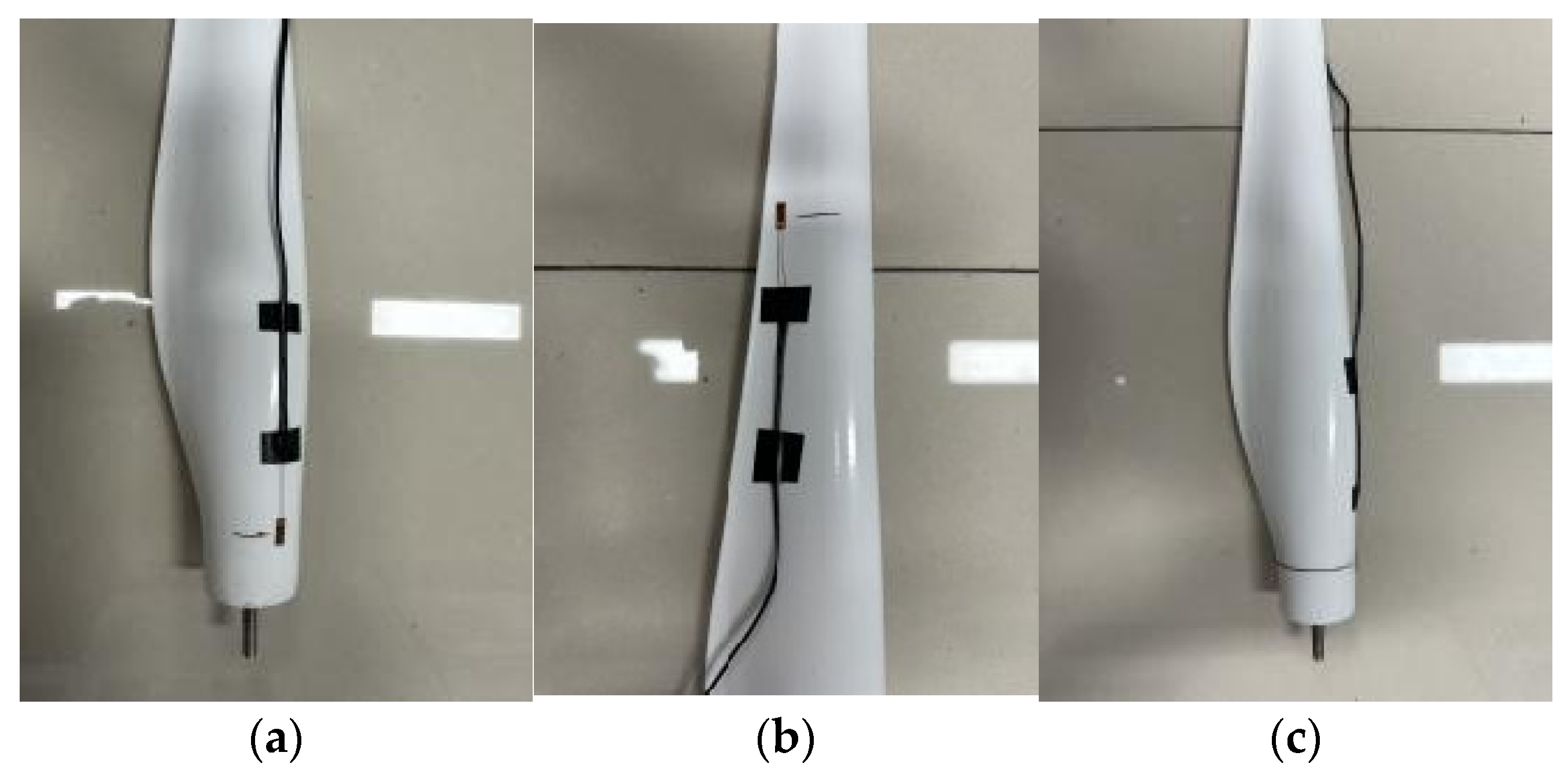
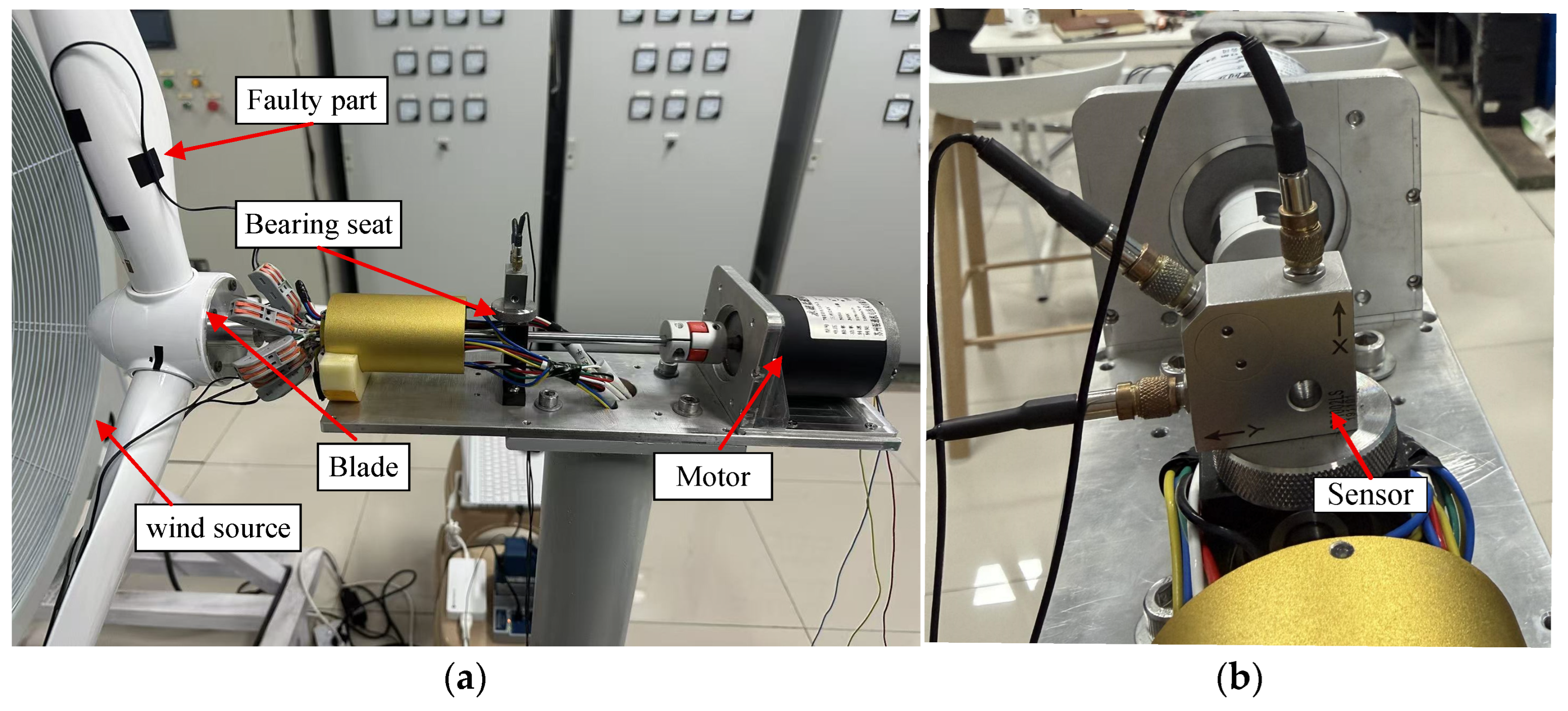
This research utilized the double-fed wind turbine scaled test rig at the National Key Laboratory for Offshore Wind Turbine Equipment and High-Efficiency Utilization of Wind Energy (Figure 1a) to conduct simulation experiments on blade crack faults. The objective was to gather vibration response data under varying crack positions and lengths, thereby elucidating the intrinsic mapping relationship between crack characteristics and the three-dimensional vibration of the blade root bearing housing. The physical parameters of the test blades are shown in

Table 1. The physical parameters of the test blade.

Parameter	Value
Material density (kg/m3)	1000
Modulus of elasticity (MPa)	3200
Moment of inertia of cross-section (m4)	0.92 × 10−9
Blade length (m)	0.6

. The crack fault specimens were fabricated by pre-forming scratches on the surface of the test blade, with both the width and depth of the scratches controlled to be within 1 mm (inclusive), as depicted in Figure 2 and detailed in

Table 2. Description of prefabricated fault components.

Label	Failure Mode	Location	Crack Length	Image
F1	Healthy
F2	Crack	Root crack	10 mm	Figure 2a
F3	Crack	Central crack	20 mm	Figure 2b
F4	Crack	Root crack	30 mm	Figure 2c

. Throughout the experiment, a CT1010LS piezoelectric three-axis IEPE vibration acceleration sensor from Yangzhou KEDONG Electronics Co., Ltd. (Yangzhou, Jiangsu, China), was mounted on the surface of the blade root bearing housing (Figure 1b) to enable synchronous acquisition of three-dimensional vibration signals. Data collection was performed using a NI-9263 32-channel 16-bit high-speed data acquisition card from National Instruments (Austin, TX, USA), with the sampling frequency set at 10 kHz. Acquisition control and data storage were managed by a data acquisition software independently developed on the LabView 2025 platform.

The blade damage simulation experiment was designed in accordance with the actual operating conditions of a specific type of doubly fed wind turbine. Three rotational speed levels were established at 10 rpm, 20 rpm, and 30 rpm, with the speed control deviation kept within ±1 rpm. For each fault state at every speed level, five independent replicate tests were performed, each with a sampling duration of 60 s. The acquired raw data were segmented using a 1 s time window (equivalent to 10,000 sampling points), from which 1024 consecutive data points were randomly selected from each segment to form a sample. These samples were subsequently aggregated and mixed according to the fault mode. Following this processing, a total of 960 sample sets were obtained for each fault mode, collectively constituting the experimental sample set. The sample set was then partitioned into training, validation, and test sets in a 6:2:2 ratio, as detailed in

Table 3. Fault pattern and data sample length.

Fault Pattern	Sample Length	Training Set	Validation Set	Test Set
F1	1024 points	540	180	180
F2		540	180	180
F3		540	180	180
F4		540	180	180

.

2.2. Vibration Response Analysis

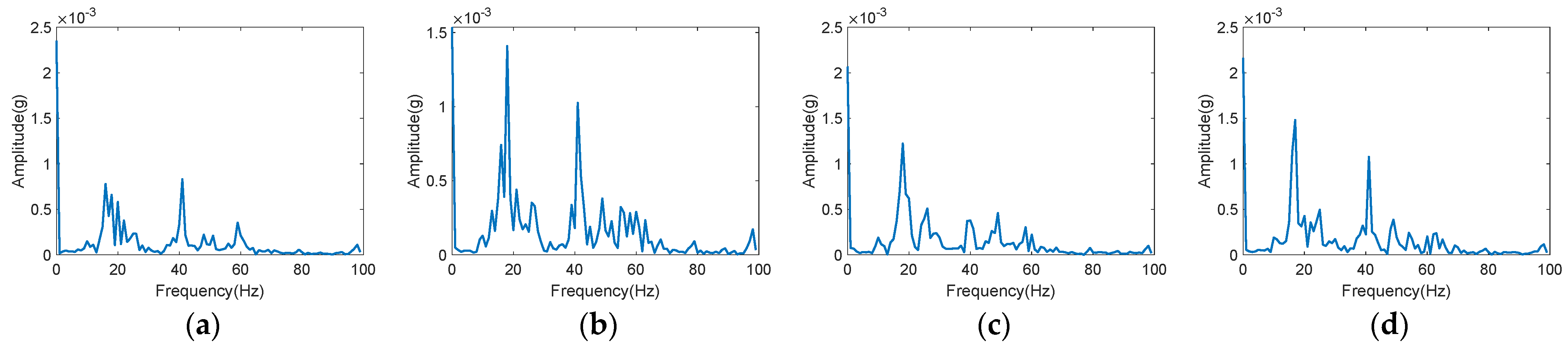
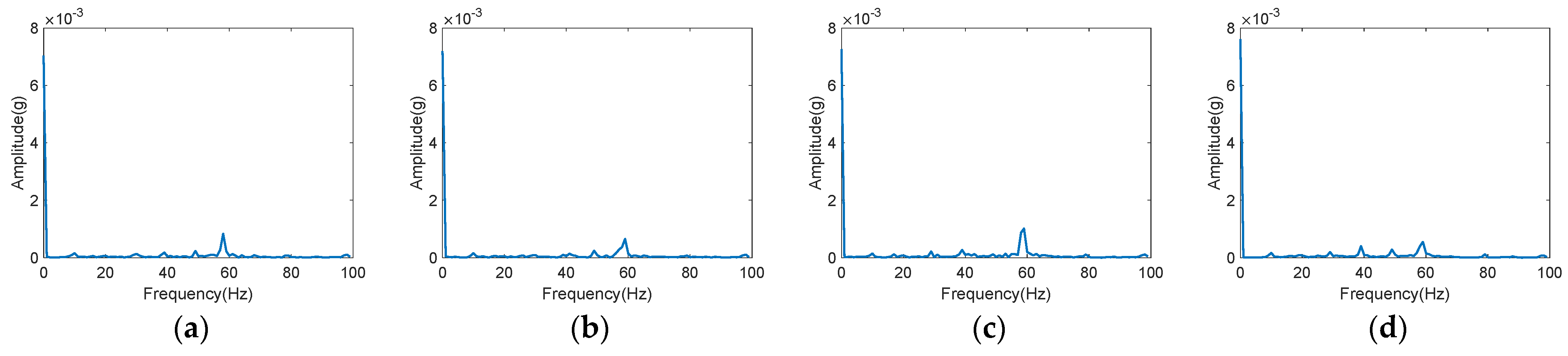
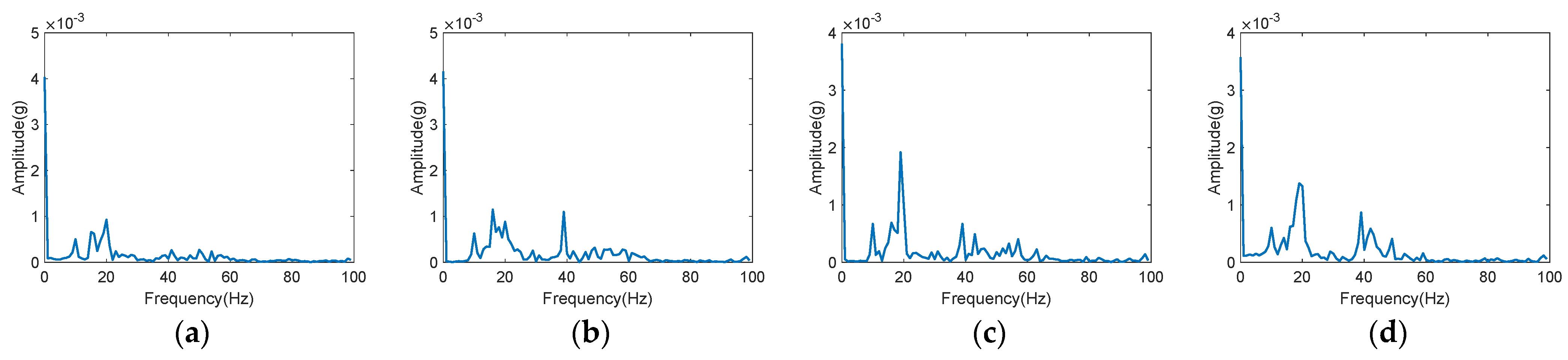
Using the operating condition with a rotational speed of 30 rpm as an illustrative example, this research analyzed the correlation between crack characteristics and the three-directional vibration response of the blade root bearing housing. The frequency spectra of the three-directional vibration signals under four distinct fault modes are presented in Figure 3, Figure 4 and Figure 5, respectively.

A comparison of Figure 3, Figure 4 and Figure 5 reveals that the three-directional vibration response of the blade root bearing exhibits pronounced directional dependence. This phenomenon fundamentally stems from the directional anisotropy in the distribution of structural stiffness and the paths of load transfer. The X-direction, being axial, benefits from high constraint stiffness provided by the bearing and locking mechanism, rendering it resistant to significant axial displacement induced by external excitation. Consequently, its frequency spectrum is relatively simple, with energy predominantly concentrated around natural frequencies associated with the rotational frequency. When cracks manifest in the blade, given that they primarily compromise bending stiffness while exerting a limited impact on axial stiffness, and considering the difficulty in exciting nonlinear responses along the axial path, the frequency spectrum in the X-direction undergoes minimal alteration, with linear responses continuing to predominate. In contrast, the Y-direction (flapping) and Z-direction (oscillation) are directly subjected to broadband dynamic loads, including aerodynamic thrust, alternating gravity, and centrifugal force components. Furthermore, the support stiffness in these two directions is comparatively lower, accompanied by an increased presence of gaps or flexible links, which are conducive to exciting higher-order structural modes. As a result, their vibration signals inherently encompass a wealth of frequency components. Following the emergence of cracks, bending stiffness further diminishes, and the cracks alternately “open” and “close” with each load cycle, resulting in nonlinear stiffness modulation. This, in turn, induces a notable increase in the amplitudes of higher-order harmonics and sidebands within the acceleration spectrum. It is evident that vibrations in the Y-direction and Z-direction exhibit heightened sensitivity to blade damage, and their harmonic and sideband characteristics can serve as pivotal indicators for the early detection of cracks. To this end, the development of a physical mapping model that integrates vibration amplitude with crack geometry and location parameters facilitates inverse inference from the vibration feature space to the crack parameter space, thereby enhancing the sensitivity and localization accuracy of blade anomaly detection.

3. PINN Modeling for Damage Identification of Wind Turbine Blades

3.1. Basic Theory of PINN

Building upon existing research on neural networks, Jo et al. [40] introduced a deep learning algorithm framework that integrates physical information, with the objective of enhancing its applicability in mathematical and physical modeling as well as engineering computations. The crux of this framework lies in harnessing the robust function approximation capabilities of neural networks while incorporating physical information as constraints to bolster the model’s physical consistency and generalization performance. By integrating prior knowledge, such as partial differential equations, conservation laws, or constraints derived from physical experiments, into conventional data-driven models, this approach effectively mitigates overfitting and enhances predictive performance for unseen data. The neural network thus trained not only accurately approximates observed values but also inherently adheres to fundamental physical laws, including symmetry, invariance, conservation, and monotonicity, as encapsulated by partial differential equations [41].

The architecture of PINN primarily comprises two components: the neural network module, which is employed for function approximation; and the physical rule module, which imposes constraints. The latter orchestrates the model training process by integrating physical laws (e.g., governing equations and conservation laws) as regularization terms within the loss function [42].

The loss function of PINN is composed of a weighted combination of data fitting term $L_{data}$, physical constraint term $L_{physics}$, and boundary condition term $L_{boundary}$. Its general form can be expressed as:

$$Loss={\lambda }_1{L}_{data}+{\lambda }_2{L}_{physics}+{\lambda }_3{L}_{boundary}$$

(1)

where ${\lambda }_i\left(i=1,2,3\right)$ is the weight coefficient used to coordinate the relative importance between data fitting and adherence to physical laws.

3.2. Physical Information Constraint Model

3.2.1. Crack-Vibration Correlation Information

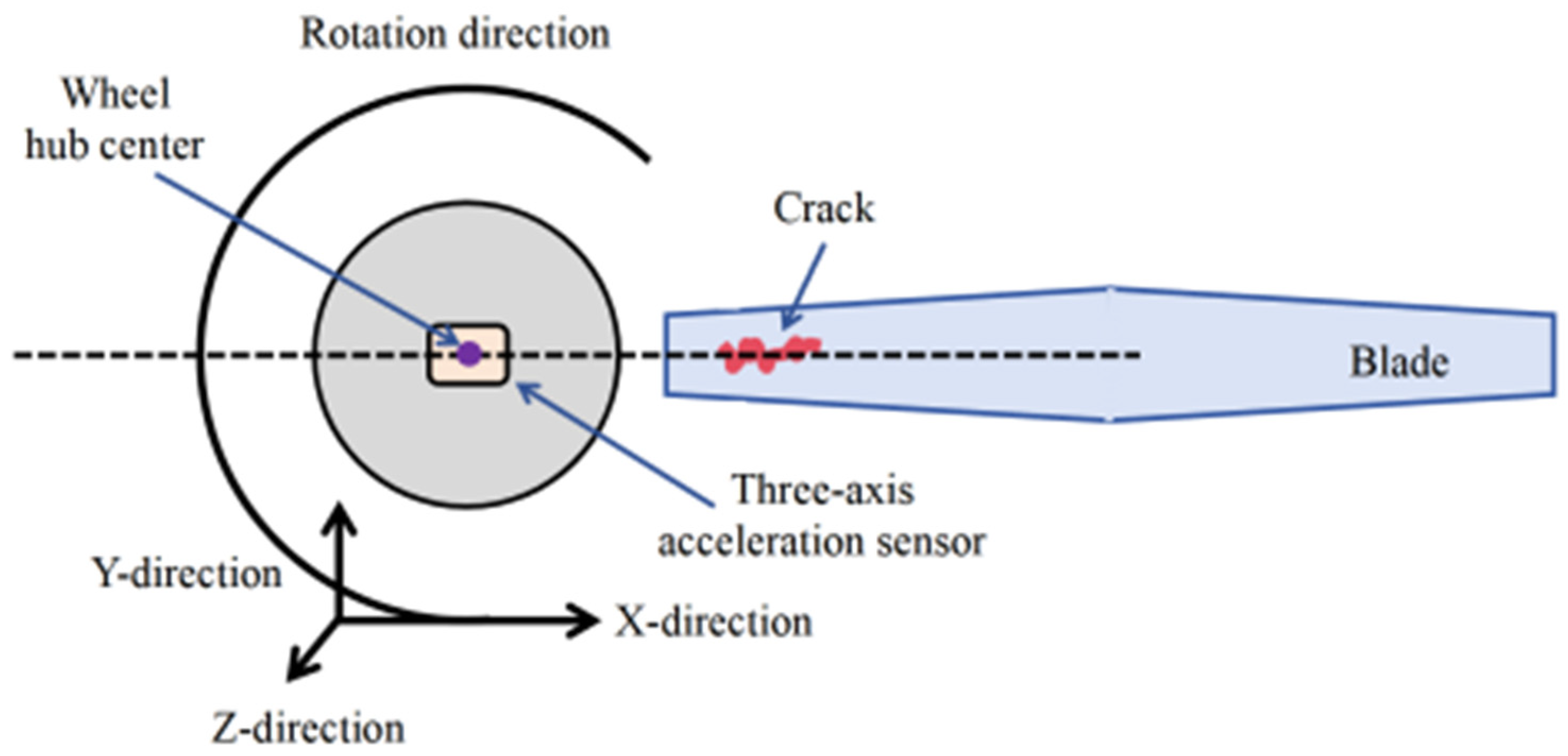
The wind turbine blade was simplified by employing the rotating cantilever Euler–Bernoulli beam model [43], as depicted in Figure 6. Within this model, the blade is considered as a uniform cross-section beam with a length denoted as $L$ and a cross-sectional area of $A$. The root of the blade is firmly attached to the hub and rotates at a constant angular velocity $\mathsf{\Omega }$ around the axis of rotation.

The variable separation method was employed to first analyze the vibrational acceleration in the flapping direction (Y-direction). Assuming the displacement in the Y-direction is denoted as $y\left(x,t\right)=\varphi \left(x\right)e^{i\omega t}$, the crack was simplified to a massless torsional spring model [44]. That is, a torsional spring was introduced at the crack position $x_c$, and the relationship between its Y-direction stiffness $K_T^{\left(y\right)}$ and crack length $a$ is:

$$K_T^{\left(y\right)}\left(a\right)={\displaystyle \frac{E{I}^{\left(y\right)}}{ah}}·{\left({\displaystyle \frac{h}{a}}\right)}^2$$

(2)

where $E{I}^{\left(y\right)}$ is the bending stiffness of the beam in the Y-direction, and $h$ is the section height of the blade. This formula indicates that the longer the crack, the more severe the decrease in local stiffness, and it is inversely proportional to $a^2$.

By treating cracks as perturbations to an intact (or undamaged) beam and based on the first-order perturbation theory [45], the i-th natural flapping frequency of a cracked beam can be formulated as:

$${\omega }_i^{\left(y\right)}\left(a,x_c\right)={\omega }_{0i}^{\left(y\right)}\sqrt{1-{\Delta }_i^{\left(y\right)}\left(a,x_c\right)}$$

(3)

where ${\omega }_{0i}^{\left(y\right)}$ is the natural flapping frequency of a healthy beam, and the frequency drop rate ${\Delta }_i^{\left(y\right)}$ is defined as:

$${\Delta }_i^{\left(y\right)}\left(a,x_c\right)={\displaystyle \frac{E{I}^{\left(y\right)}}{2{\left({\omega }_{0i}^{\left(y\right)}\right)}^2}}·{\displaystyle \frac{{\left[{\varphi }_{0i}^{″}\left(x_c\right)\right]}^2}{M_i}}·\left({\displaystyle \frac{E{I}^{\left(y\right)}}{K_T^{\left(y\right)}\left(a\right)}}\right)$$

(4)

where ${\varphi }_{0i}^{″}\left(x_c\right)$ is the curvature of the healthy mode shape in the Y-direction at the crack, and denotes the modal mass. Equation (4) reveals an important physical law, stating that the decrease in frequency is proportional to the square of the curvature of the mode shape at the crack. This relationship explains why root cracks have a more significant impact than tip cracks.

The vibration mode in the Y-direction of a cracked beam can be represented as the sum of the healthy vibration mode ${\varphi }_{i0}$ in the Y-direction and the local perturbation induced by the cracks:

$${\varphi }_i\left(x\right)={\varphi }_{0i}\left(x\right)+{\displaystyle \frac{E{I}^{\left(y\right)}}{K_T^{\left(y\right)}\left(a\right)}}·{\varphi }_{0i}^{″}\left(x_c\right)·G_i\left(x,x_c\right)$$

(5)

where $G_i\left(·\right)$ is the Green’s function, indicating the response caused by the unit corner action at $x_c$.

When subjected to external load $f\left(x,t\right)=F\left(x\right)e^{i\mathsf{\Omega }t}$, the modal coordinate $q_i^{\left(y\right)}\left(t\right)$ conforms to the following condition based on the modal superposition method [45]:

$${\ddot{q}}_i^{\left(y\right)}+2{\varsigma }_i{\omega }_i^{\left(y\right)}{\dot{q}}_i^{\left(y\right)}+{\left({\omega }_i^{\left(y\right)}\right)}^2{q}_i^{\left(y\right)}={\displaystyle \frac{Q_i^{\left(y\right)}}{M_i}}{e}^{i\mathsf{\Omega }t}$$

(6)

where ${\varsigma }_i$ is the damping ratio of the i-th mode, and the modal force $Q_i^{\left(y\right)}$ in the Y-direction can also be decomposed into two parts: healthy and crack disturbance.

$$Q_i^{\left(y\right)}=Q_{0i}^{\left(y\right)}+{\displaystyle \frac{E{I}^{\left(y\right)}}{K_T^{\left(y\right)}\left(a\right)}}·{\varphi }_{0i}^{″}\left(x_c\right)·{\Gamma }_i\left(x_c\right)$$

(7)

where ${\Gamma }_i\left(x_c\right)={\displaystyle {\int }_0^{L}F\left(x\right)}·G_i\left(x,x_c\right)dx$ is the influence integral of the crack location.

Substituting Equation (7) into Equation (6), the steady-state solution for $q_i^{\left(y\right)}(t)$ is:

$$q_i^{\left(y\right)}\left(t\right)={\displaystyle \frac{Q_i^{\left(y\right)}·H_i^{\left(y\right)}}{M_i}}{e}^{i\mathsf{\Omega }t}$$

(8)

where $H_i^{\left(y\right)}$ is the frequency response function of the i-th mode.

$$H_i^{\left(y\right)}={\displaystyle \frac{1}{{\left({\omega }_i^{\left(y\right)}\right)}^2-{\mathsf{\Omega }}^2+2j{\varsigma }_i{\omega }_i^{\left(y\right)}\mathsf{\Omega }}}$$

(9)

The displacement in the Y-direction at the hub center is denoted as $y\left(0,t\right)={\displaystyle \sum _i{\varphi }_i\left(0\right)q_i^{\left(y\right)}\left(t\right)}$. Substituting Equations (5) and (8) yields the amplitude of the sensor’s acceleration in the Y-direction as follows:

$$A_y={\mathsf{\Omega }}^2\left|{\displaystyle \sum _i\frac{E{I}^{\left(y\right)}}{K_T^{\left(y\right)}\left(a\right)}·{\varphi }_{0i}^{″}\left(x_c\right)·G_i\left(x,x_c\right)·\frac{Q_{0i}^{\left(y\right)}+\frac{E{I}^{\left(y\right)}}{K_T^{\left(y\right)}\left(a\right)}·{\varphi }_{0i}^{″}\left(x_c\right)·{\Gamma }_i\left(x_c\right)}{M_i}·H_i^{\left(y\right)}}\right|$$

(10)

Similarly, the acceleration amplitude in the Z-direction (blade flutter direction) can be calculated based on the healthy mode shape ${\phi }_{i0}$ in this direction and its corresponding slope ${\phi }_{i0}^{″}$ at the crack location:

$$A_z={\mathsf{\Omega }}^2\left|{\displaystyle \sum _i\frac{E{I}^{\left(z\right)}}{K_T^{\left(z\right)}\left(a\right)}·{\phi }_{0i}^{″}\left(x_c\right)·G_i\left(x,x_c\right)·\frac{Q_{0i}^{\left(z\right)}+\frac{E{I}^{\left(z\right)}}{K_T^{\left(z\right)}\left(a\right)}·{\phi }_{0i}^{″}\left(x_c\right)·{\Gamma }_i\left(x_c\right)}{M_i}·H_i^{\left(z\right)}}\right|$$

(11)

where $K_T^{\left(z\right)}$ is the stiffness of the beam in the Z-direction, $E{I}^{\left(z\right)}$ is the bending stiffness in the Z-direction, $Q_i^{\left(z\right)}$ is the modal force in the Z-direction, and $H_i^{\left(z\right)}$ is the frequency response function in the Z-direction.

Vibration in the X-direction (axial direction) mainly stems from the longitudinal shortening effect caused by bending:

$$A_x=4{\mathsf{\Omega }}^2\left|{\displaystyle \sum _i{\Lambda }_i{\left(a,x_c\right)}^2\left(\frac{Q_i^{\left(x\right)}·H_i^{\left(x\right)}}{M_i}\right)}\right|$$

(12)

where $Q_i^{\left(x\right)}$ is the modal force in the X-direction, $H_i^{\left(x\right)}$ denotes the frequency response function in the X-direction, and ${\Lambda }_i$ signifies the axial strain coefficient of the i-th mode. Under the small crack condition (${\displaystyle \frac{a}{h}}<<1$), the scenario can be approximated as:

$${\Lambda }_i\left(a,x_c\right)={\Lambda }_{0i}\left[1+{\alpha }_i{\displaystyle \frac{E{I}^{\left(x\right)}}{K_T^{\left(x\right)}\left(a\right)}}{\eta }_{0i}^{″}\left(x_c\right)\right]$$

(13)

where ${\eta }_{0i}^{″}\left(x_c\right)$ is the curvature of the healthy mode shape ${\eta }_{0i}$ in the X-direction at the crack location, while ${\alpha }_i$ denotes the dimensionless axial modal coupling coefficient, with a value ranging from 0.1 to 2.0, depending on the modal order and crack location.

3.2.2. Modeling of Physical Information Constraint

To develop a physical information-constrained model for crack-vibration analysis, the expression for acceleration amplitude was simplified with consideration of the following factors:

(1)

Within the modeling frequency band, the blade predominantly exhibits first-order modal response, while the root response of higher-order modes remains weak due to weaker excitation. Consequently, the influence of higher-frequency modes is disregarded.

(2)

Under conditions of small cracks, the torsional spring stiffness associated with the crack is notably high, rendering the crack disturbance term in the modal force a second-order minor quantity. Thus, the crack disturbance term in the modal force is omitted, and only the mode shape disturbance term is preserved.

(3)

The magnitudes of sway and flutter frequencies are comparable, with the axial response being the outcome of squared coupling of the flutter mode and inheriting its frequency characteristics from the flutter. Therefore, by overlooking the differences in natural frequencies across directions and assuming that the first-order frequencies in all three directions are ${\omega }_1^{\left(y\right)}={\omega }_1$, the result $H_1^{\left(x\right)}=H_1^{\left(y\right)}=H_1^{\left(z\right)}=H_1$ is obtained.

Based on the aforementioned assumptions, Equations (10)–(12) are decomposed into the product of independent functions concerning crack length $a$, crack position $x_c$, and frequency ${\omega }_1$:

$$A_y\left(\mathsf{\Omega };a,x_c\right)={\mathsf{\Omega }}^2·C_y·f_y\left(a\right)·g_y\left(a\right)·\left|H_1\left(\mathsf{\Omega };a,x_c\right)\right|$$

(14)

$$A_z\left(\mathsf{\Omega };a,x_c\right)={\mathsf{\Omega }}^2·C_z·f_z\left(a\right)·g_z\left(a\right)·\left|H_1\left(\mathsf{\Omega };a,x_c\right)\right|$$

(15)

$$A_x\left(\mathsf{\Omega };a,x_c\right)=4{\mathsf{\Omega }}^2·C_x·\left|H_1\left(\mathsf{\Omega };a,x_c\right)\right|$$

(16)

where $C_x={\Lambda }_{01}{\left({\displaystyle \frac{Q_{01}^{\left(x\right)}}{M_1}}\right)}^2$, $C_y={\displaystyle \frac{Q_{01}^{\left(y\right)}}{M_1}}$, and $C_z={\displaystyle \frac{Q_{01}^{\left(z\right)}}{M_1}}$ are the proportionality constants for the X-, Y-, and Z-directions, respectively. $f_y\left(a\right)={\displaystyle \frac{E{I}^{\left(y\right)}}{K_T^{\left(y\right)}\left(a\right)}}$ and $f_y\left(a\right)={\displaystyle \frac{E{I}^{\left(z\right)}}{K_T^{\left(z\right)}\left(a\right)}}$ are the crack length influence functions for the Y- and Z-directions, and $g_y\left(x_c\right)=\left|{\varphi }_{01}^{″}\left(x_c\right)G_1\left(0,x_c\right)\right|$ and $g_z\left(x_c\right)=\left|{\phi }_{01}^{″}\left(x_c\right)G_1\left(0,x_c\right)\right|$ are the crack position influence functions for the Y- and Z-directions.

Further analysis of ${\omega }_1$ reveals that, based on the perturbation results of the first-order mode, under the condition of small cracks, the following holds:

$${\omega }_1\left(\mathsf{\Omega };a,x_c\right)={\omega }_{01}\sqrt{1+{\displaystyle \frac{{\mathsf{\Omega }}^2}{{\omega }_{01}^2}}{J}_1}·\left[1-{\displaystyle \frac{1}{2}}\gamma \left(x_c\right){\left({\displaystyle \frac{a}{h}}\right)}^2\right]$$

(17)

where ${\omega }_{01}$ is the first-order natural frequency of a healthy beam, $J_1$ denotes the first-order rotational stiffening coefficient, and $\gamma \left(x_c\right)$ signifies the influence coefficient of crack location on frequency. $\left|H_1\left(\mathsf{\Omega };a,x_c\right)\right|$ is calculated based on Formula (17):

$$\left|H_1\left(\mathsf{\Omega };a,x_c\right)\right|={\displaystyle \frac{1}{{\left[{\omega }_{01}^2\left(1-\gamma \left(x_c\right){\left(a/h\right)}^2\right)+J_1{\mathsf{\Omega }}^2-{\mathsf{\Omega }}^2\right]}^2+{\left(2{\varsigma }_1{\omega }_{01}\sqrt{1+J_1{\mathsf{\Omega }}^2/{\omega }_{01}^2}·\mathsf{\Omega }\right)}^2}}$$

(18)

Substitute Equation (18) into Equations (14)–(16) to establish a physical information constraint model for crack-vibration:

$$A_y\left(\mathsf{\Omega };a,x_c\right)={\displaystyle \frac{C_y·f_y\left(a\right)·g_y(x_c)·{\mathsf{\Omega }}^2}{{\left[{\omega }_{01}^2\left(1-\gamma \left(x_c\right){\left(a/h\right)}^2\right)+J_1{\mathsf{\Omega }}^2-{\mathsf{\Omega }}^2\right]}^2+{\left(2{\varsigma }_1{\omega }_{01}\sqrt{1+J_1{\mathsf{\Omega }}^2/{\omega }_{01}^2}·\mathsf{\Omega }\right)}^2}}$$

(19)

$$A_z\left(\mathsf{\Omega };a,x_c\right)={\displaystyle \frac{C_z·f_z\left(a\right)·g_z(x_c)·{\mathsf{\Omega }}^2}{{\left[{\omega }_{01}^2\left(1-\gamma \left(x_c\right){\left(a/h\right)}^2\right)+J_1{\mathsf{\Omega }}^2-{\mathsf{\Omega }}^2\right]}^2+{\left(2{\varsigma }_1{\omega }_{01}\sqrt{1+J_1{\mathsf{\Omega }}^2/{\omega }_{01}^2}·\mathsf{\Omega }\right)}^2}}$$

(20)

$$A_x\left(\mathsf{\Omega };a,x_c\right)={\displaystyle \frac{4C_x·{\mathsf{\Omega }}^2}{{\left[{\omega }_{01}^2\left(1-\gamma \left(x_c\right){\left(a/h\right)}^2\right)+J_1{\mathsf{\Omega }}^2-{\mathsf{\Omega }}^2\right]}^2+{\left(2{\varsigma }_1{\omega }_{01}\sqrt{1+J_1{\mathsf{\Omega }}^2/{\omega }_{01}^2}·\mathsf{\Omega }\right)}^2}}$$

(21)

3.3. PINN Modeling

3.3.1. GRU-Transformer Network

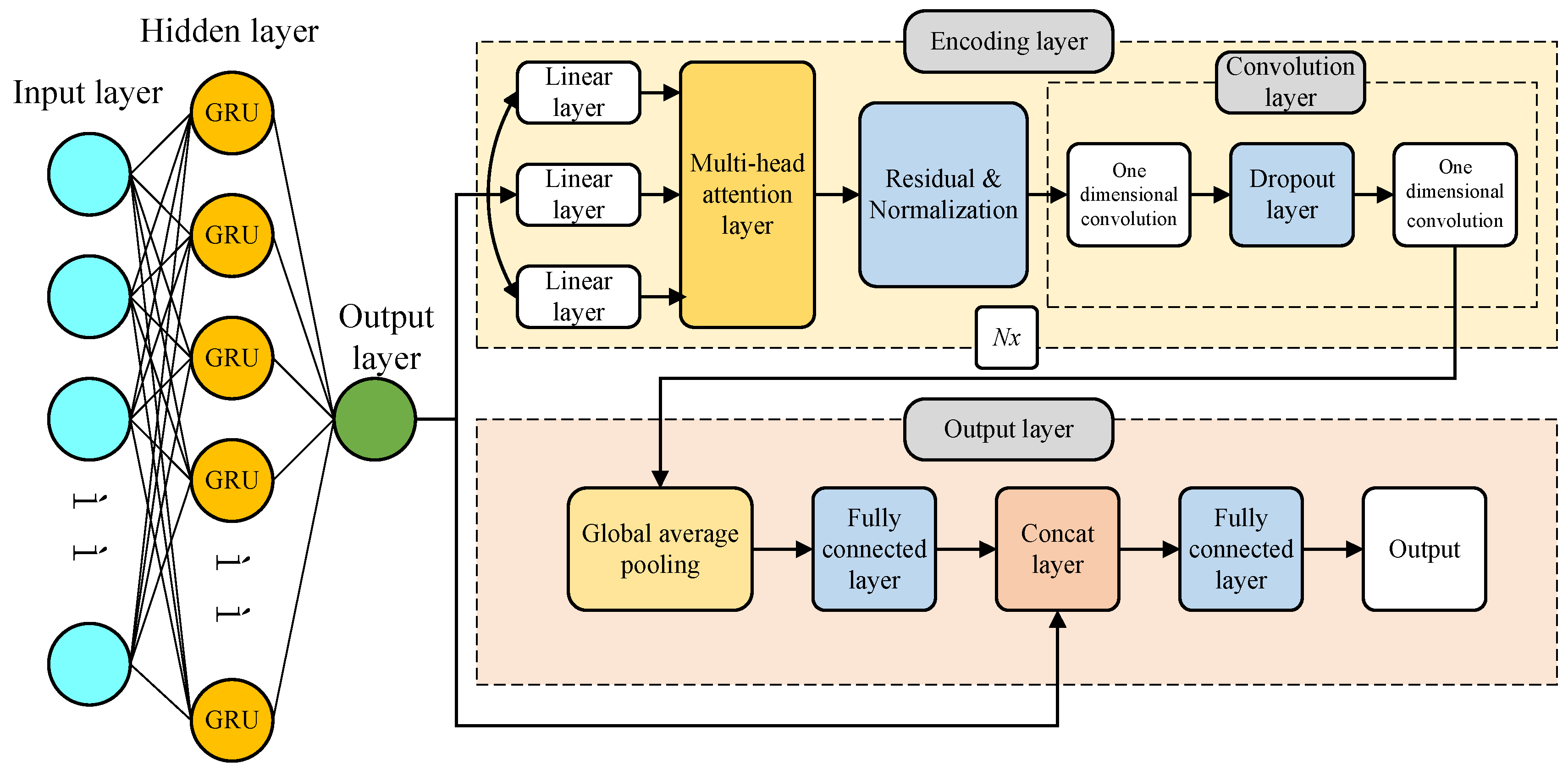
In this research, GRU-Transformer was selected as the deep learning network for blade damage identification [46,47], as shown in Figure 7.

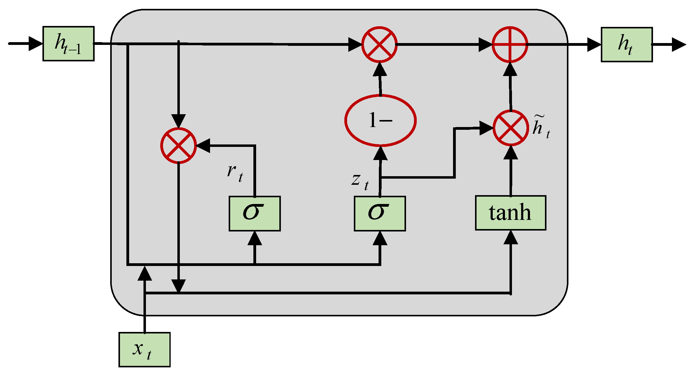
The Gated Recurrent Unit-Transformer (GRU) represents a streamlined variant of the Long Short-Term Memory (LSTM) network. It effectively mitigates the vanishing gradient issue inherent in conventional recurrent neural networks (RNNs) by employing update and reset gate mechanisms, enabling adaptive capture of short-term dependencies within time-series data. Notably, it offers the benefits of reduced parameter quantity and accelerated training speed. The GRU neuron is composed of an update gate and a reset gate, as illustrated in Figure 8.

At time $t$, the internal state of the GRU neuron is represented as follows:

$$r_t=\sigma \left(U_r{x}_t+W_r{h}_{t-1}+b_r\right)$$

(22)

$$z_t=\sigma \left(U_z{x}_t+W_z{h}_{t-1}+b_z\right)$$

(23)

$$h_t=\tanh \left(U_h{x}_t+W_h\left(r_t\otimes h_{t-1}\right)+b_h\right)$$

(24)

$$h_t=\left(1-z_t\right)\otimes h_{t-1}+z_t\otimes h_t$$

(25)

where $x_t$ is the input data at time $t$; $r_t$ and $z_t$ are the outputs of the reset gate and update gate respectively; $h_t$ is the hidden state; $U$, $W$, and $b$ are the weight and bias matrices respectively; $\sigma$ is the Sigmoid activation function; and ${\tilde{h}}_t$ is the temporary hidden state.

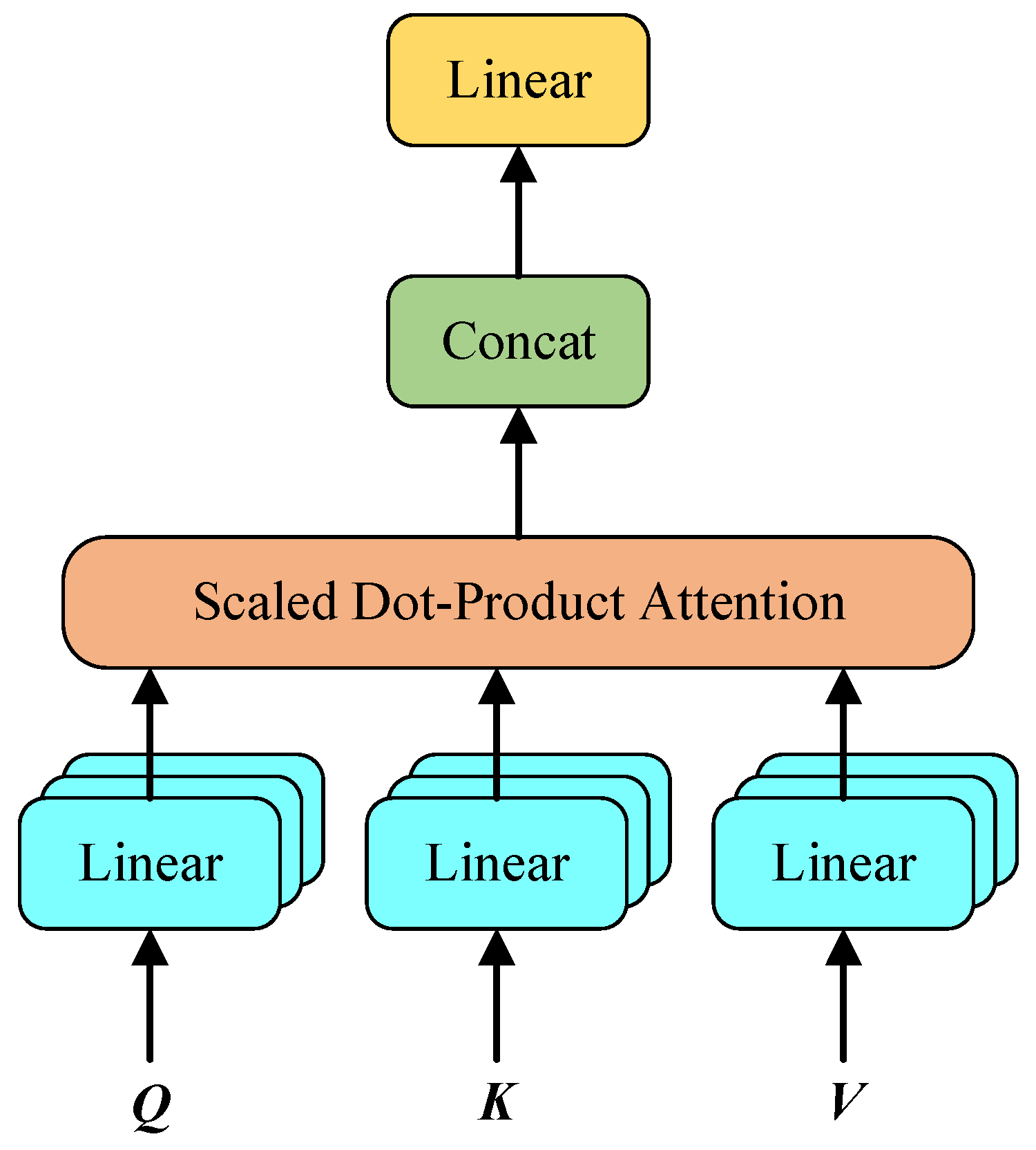
Transformer is entirely constructed based on the self-attention mechanism, abandoning the recurrent structure. It captures long-range dependencies at any position in the sequence through parallel multi-head attention. Its positional encoding mechanism enables the model to perceive temporal order, and it excels in global feature modeling. The computational process of the multi-head self-attention mechanism is illustrated in Figure 9.

For the input sequence $X\in R^{n\times d}$, the attention score of the i-th element $x_i$ can be expressed as:

$$Attension(Q,K,V)=soft\max \left({\displaystyle \frac{Q{K}^T}{\sqrt{d_k}}}\right)V$$

(26)

where $Q$, $K$, and $V$ are the query matrix, key matrix, and value matrix, respectively, while $d_k$ denotes the scaling factor.

The multi-head attention mechanism can be represented as:

$$MultiHeal(Q,K,V)=Concat(hea{d}_1,hea{d}_2,\cdots ,hea{d}_h)W^o$$

(27)

$$hea{d}_i=Attension(Q{W}_i^Q,K{W}_i^K,V{W}_i^V)$$

(28)

where $W^O\in R^{h{d}_k\times d}$ is the output weight matrix, while $W_i^Q$, $W_i^K$, and $W_i^V$ are the learnable weight matrices for $Q$, $K$, and $V$, respectively.

Combining GRU and Transformer can complement each other’s strengths: GRU serves as a preprocessing layer to perform preliminary filtering and dimensionality reduction on the input sequence, extracting key short-term fluctuation features and compressing the sequence length; Transformer, on this basis, utilizes the multi-head attention mechanism to deeply explore global dependencies. This combined architecture of “GRU local perception + Transformer global modeling” not only retains the efficiency of GRU in processing short-term patterns but also fully utilizes the powerful capabilities of Transformer in long sequence modeling, significantly improving the model’s prediction accuracy for complex time-series signals while maintaining low computational overhead.

The ReLU function was chosen as the activation function for the GRU-Transformer network, and the physical model is trained based on experimental data, using cross-entropy loss as the loss function. During the model training process, the K-fold cross-validation method [48] is employed to adjust the model hyperparameters to achieve optimal diagnostic performance (K = 10). The final determined model parameters are shown in

Table 4. Parameters of GRU-Transformer network.

Network Parameters	Values
Number of GRU layers	1
Number of GRU neurons	50
Number of Transformer encoder blocks	4
Dimension of attention heads	64
Number of attention heads	16
Dimension of fully connected layer	64
Dropout rate	0.1

.

3.3.2. PINN Model for Blade Crack Damage Identification

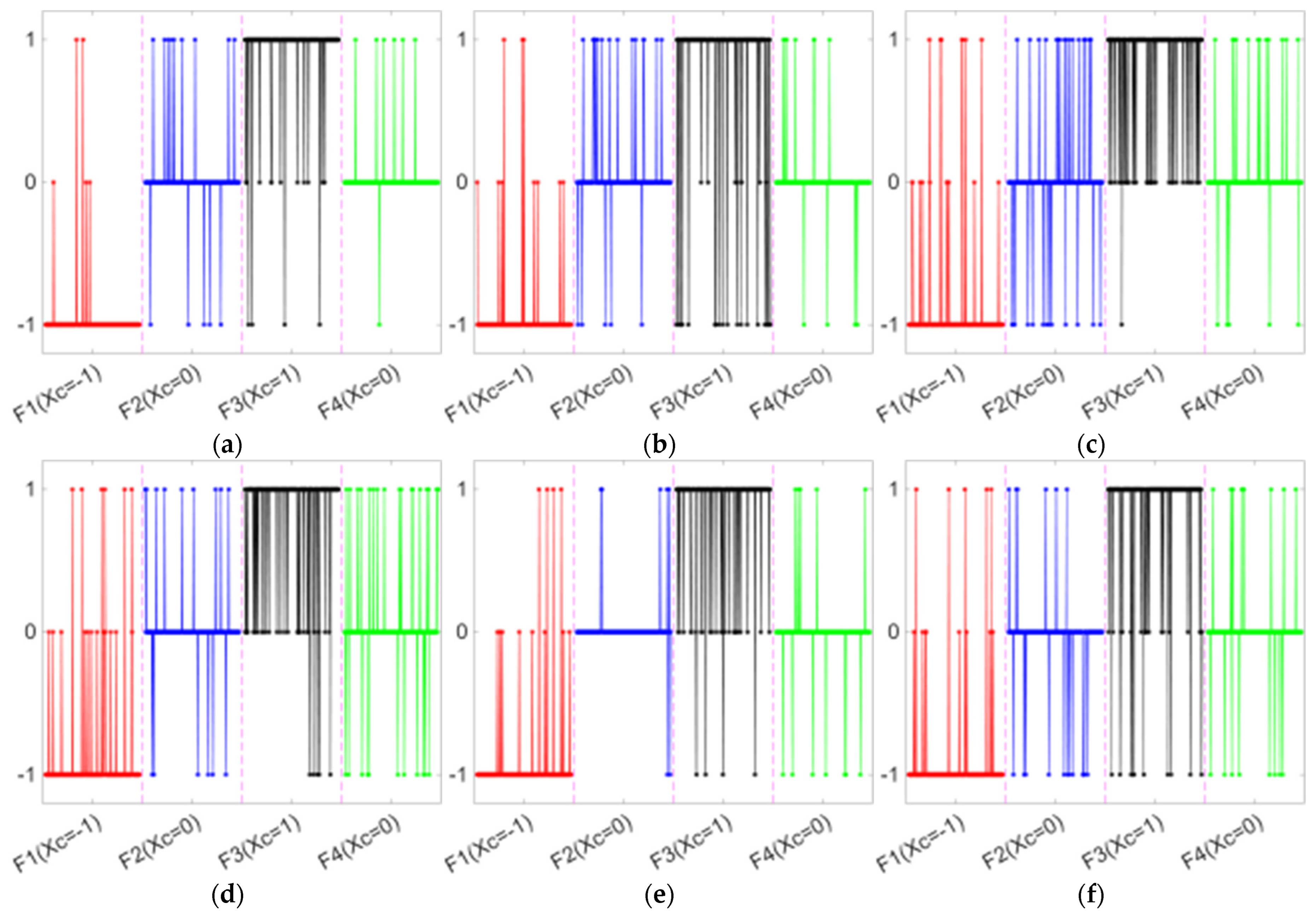
In the previously mentioned physical information-constrained model of crack-vibration, the crack position $x_c$ is represented as a continuous parameter within both the frequency influence coefficient $\gamma \left(x_c\right)$ and the position influence function $g\left(x_c\right)$. When $x_c$ is regarded as a continuous variable for regression analysis, two significant challenges emerge in practical engineering applications: Firstly, measured vibration signals inevitably incorporate noise and uncertainties, and the continuous inverse problem is inherently ill-posed. Consequently, minor measurement discrepancies can induce substantial fluctuations in position estimation. Secondly, the influence of crack position on vibration response exhibits spatial non-uniformity, with response variations being exceedingly subtle at specific locations (e.g., near mode shape nodes), thereby impeding the convergence of continuous regression models to a stable solution. To overcome these issues, this research discretized the crack position x_c into three representative states: crack-free (x_c = −1), root crack (x_c = 0), and central crack (x_c = 1). This approach transforms the originally sensitive continuous inverse problem into a more robust three-class classification problem, substituting precise localization with fault pattern recognition, and thus enabling reliable diagnosis within an engineering-acceptable accuracy margin.

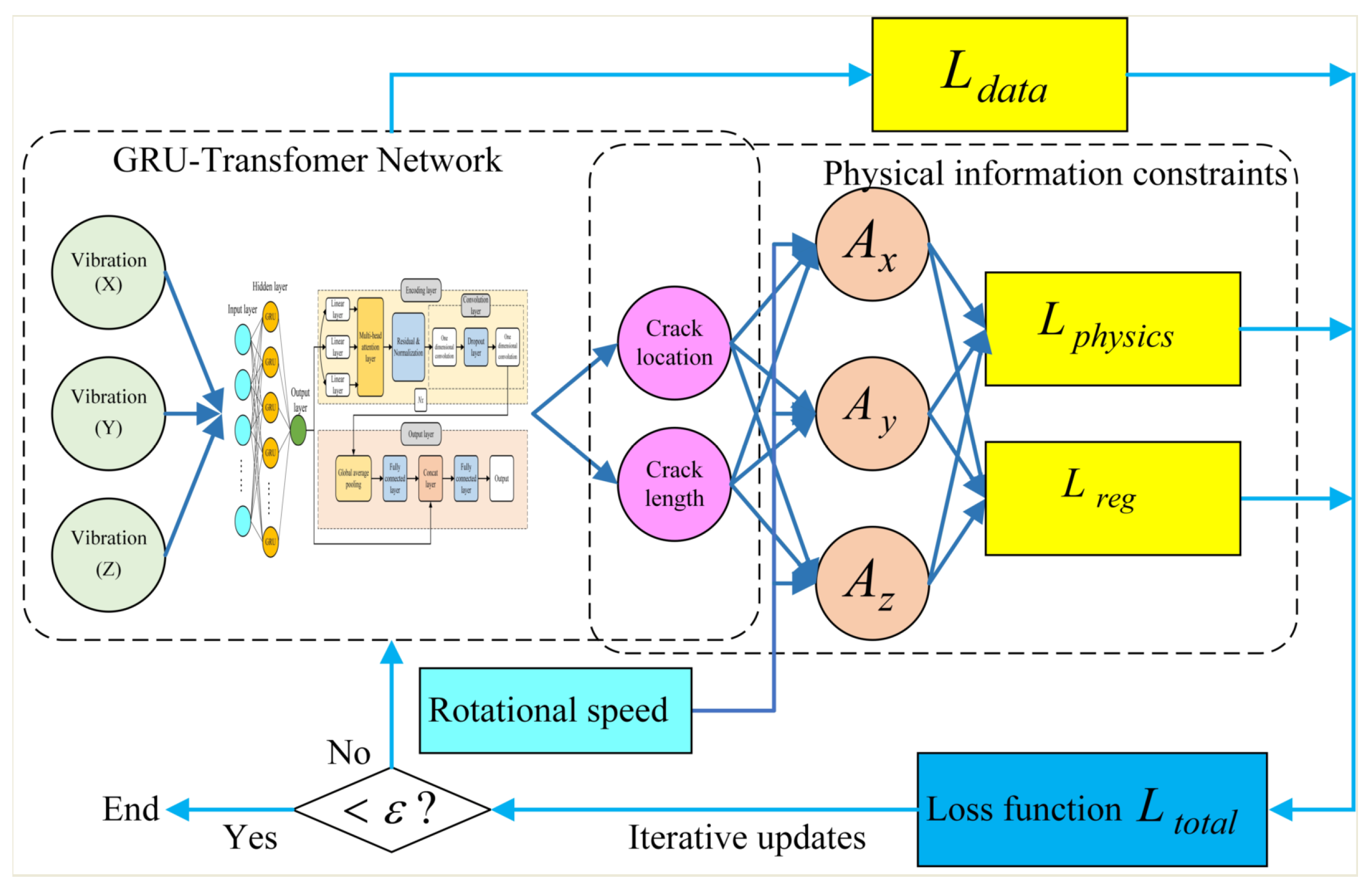
Based on the aforementioned discretization strategy, the physical information constraint model of wind turbine blade cracks and vibration in Section 3.2.2 is integrated into the GRU-Transformer network to construct a blade damage identification model based on PINN, as shown in Figure 10. Specifically, the input dimension of the model is three-dimensional, representing vibration accelerations in three directions, and the output layer dimension is two-dimensional, encompassing crack length $a$ and crack position $x_c$, respectively.

The loss function of the model comprises multiple components, among which the error loss term arising from data fitting is:

$$L_{data}={\displaystyle \frac{1}{N}}{\displaystyle \sum _{j=1}^N\left[{\left(a_j^{pred}-a_j^{true}\right)}^2+{\left(x_{c,j}^{pred}-x_{x,j}^{true}\right)}^2\right]}$$

(29)

where $N$ is the data length, $a_j^{true}$ and $x_{c,j}^{true}$ denote the normalized labels of crack length and position corresponding to the j-th sample, while $a_j^{pred}$ and $x_{c,j}^{pred}$ signify the predicted values of the j-th sample by the GRU-Transformer network.

The physical constraint loss term generated by the physical information constraint model is:

$$L_{physics}={\displaystyle \frac{1}{N}}{\displaystyle \sum _{j=1}^N{‖A^{pred}\left({\mathsf{\Omega }}_j;a_j^{pred},x_{c,j}^{pred}\right)-A_j^{measured}‖}^2}$$

(30)

where $A_j^{measured}$ is the measured acceleration amplitude value of the j-th sample, while $A^{pred}\left({\mathsf{\Omega }}_j;a_j^{pred},x_{c,j}^{pred}\right)$ denotes the network prediction value based on the j-th sample, which is calculated using Equations (19)–(21).

Finally, to ensure that the parameters learned by the model possess meaningful network insights, prevent overfitting, and guarantee the stability of predictions, a regularization loss term is constructed.

$$L_{reg}=L_{param}+L_{smooth}$$

(31)

In Equation (31), $L_{param}$ represents the physical parameter boundary constraint term, ensuring that the trainable physical parameters in the PINN model remain within a reasonable physical range:

$$L_{param}={\displaystyle \sum _{p\in P}\left[\mathrm{ReLU}\left(p_{min}-p\right)+\mathrm{ReLU}\left(p-p_{max}\right)\right]}$$

(32)

where $P$ is a set of trainable physical parameters, encompassing the directional proportionality constant $C_d$, the crack position influence function $g_d$, the crack length influence function $f_d$, and the crack position frequency influence function $\gamma$, among others, with $d=x,y,z$. Throughout the training process, all physical parameters are initialized to a value of 1.0, signifying the ideal stiffness and amplitude gain under the baseline condition of a crack-free state. To prevent parameter drift during optimization from straying beyond physically plausible bounds, the permissible range for each parameter is constrained as follows: $\gamma ,g_d\in [0.5,2.0]$, $C_d\in [0.5,3.0]$, $f_d\in [0.5,5.0]$.

$L_{smooth}$ serves as a physical regularization constraint term, designed to impose smoothness constraints on the variations of $\gamma$ and $g_d$ across different discrete states, thereby ensuring the continuity of physical parameters and mechanical plausibility during the crack evolution process.

$$L_{smooth}={‖\gamma \left(-1\right)-2\gamma \left(0\right)+\gamma \left(1\right)‖}^2+{\displaystyle \sum _{d=x,y,z}{‖g_d\left(-1\right)-2g_d\left(0\right)+g_d\left(1\right)‖}^2}$$

(33)

In summary, by weighting and summing the loss items of each part, the final loss function can be obtained as follows:

$$L_{total}={\lambda }_1{L}_{data}+{\lambda }_2{L}_{pyhsics}+{\lambda }_3{L}_{reg}$$

(34)

The model training adopts a multi-loss dynamic weighting and staged training approach, with the loss function weight coefficient ${\lambda }_i\left(i=1,2,3\right)$ also treated as a “trainable parameter” of the model, incorporated into the Adam optimizer for joint learning and dynamic adjustment [49]. A two-stage strategy is employed during the training process: Firstly, the physical model parameters are fixed and only the weights of the GRU-Transformer network are optimized. This stage involves 100 rounds of training, with a learning rate set at 0.001 and a decay of 0.2 every 50 rounds. Subsequently, the joint fine-tuning stage begins, during which the physical model parameters are unfrozen and both the network weights and physical model parameters are optimized. An early stopping mechanism is introduced in this stage to control the training process: performance on the validation set is monitored in real time. If the accuracy on the validation set does not improve for 10 consecutive rounds, training is terminated early; otherwise, training continues until reaching the preset upper limit of 300 rounds.

4. Instance Verification and Analysis

4.1. Scheme of Instance Verification

4.1.1. Test Environment and Evaluation Metrics

The wind turbine blade damage identification model that integrates PINN, as proposed in this research, was programmed and implemented on the MATLAB 2025b platform. The operating environment was equipped with an Intel i9-12900 processor (3.19 GHz) and 64 GB of RAM. The model underwent testing using experimental data derived from damage simulation experiments, and its performance in crack damage identification was evaluated through various indicators, including accuracy, coefficient of determination $E_{R^2}$, root mean square error $E_{RMSE}$, mean absolute percentage error $E_{MAPE}$, training time, floating-point operations (FLOPs), parameter quantity, model file size and inference time. Specifically, accuracy was employed to gauge the model’s precision in recognizing fault modes (where $x_c=-1$ and $x_c=1$ correspond to fault modes F1 and F3, respectively; $x_c=0$ in conjunction with $a<20$ to fault mode F2; and $x_c=0$ in conjunction with $a\ge 20$ to fault mode F4). $E_{R^2}$, $E_{RMSE}$ and $E_{MAPE}$ were utilized to assess the prediction accuracy of crack length. Meanwhile, training time, FLOPs, parameter quantity, model file size and inference time served as metrics for evaluating the model’s computational performance. The calculation formulas for some of these evaluation indicators are presented as follows [50]:

$$E_{R^2}=1-{\displaystyle \frac{{\displaystyle \sum _{i=1}^n{\left(y_i-{\widehat{y}}_i\right)}^2}}{{\displaystyle \sum _{i=1}^n{\left(y_i-{\overline{y}}_i\right)}^2}}}$$

(35)

$$E_{RMSE}=\sqrt{{\displaystyle \frac{1}{n}}{\displaystyle \sum _{i=1}^n{\left(y_i-{\widehat{y}}_i\right)}^2}}$$

(36)

$$E_{MAPE}={\displaystyle \frac{1}{n}}{\displaystyle \sum _{i=1}^n\frac{\left|y_i-{\widehat{y}}_i\right|}{{\widehat{y}}_i}}\times 100\%$$

(37)

where $n$ represents the total number of samples, $y_i$ denotes the true value of the sample, ${\widehat{y}}_i$ signifies the predicted value of the sample, and ${\widehat{y}}_i$ stands for the average of the true values of the samples.

4.1.2. Deep Learning Models for Comparative Analysis

To validate the effectiveness and superiority of the method proposed in this research for the application of damage localization and identification in wind turbine blades, a systematic comparative analysis was carried out between the PINN model and the following representative deep learning models:

(1)

GRU-Transformer: Based on the network architecture in Figure 7 and the parameters in Table 4, without considering physical constraint information;

(2)

CNN-LSTM [51]: Extract local shallow and deep features of three-dimensional vibration signals using convolutional layers, fuse them, and then input them into LSTM to capture long-range dependencies in time series;

(3)

CNN-Transformer [52]: Local feature encoding is implemented via convolutional layers, and a standard Transformer module is incorporated to facilitate global cross-stride feature interaction.

(4)

FD-Transformer [53]: Vibration signals are preprocessed using multi-channel one-dimensional convolution, and a Transformer encoder with a dense connection structure is constructed to enhance the efficiency of feature extraction;

(5)

Swin Transformer [54]: Conduct a wavelet time–frequency transformation on each vibration component, transform it into a two-dimensional time–frequency image, and subsequently feed it into a model that incorporates a hierarchical window attention mechanism to capture multi-scale spatial features.

4.2. Comparative Analysis Experiment of Model Performance

4.2.1. Model Training and Validation

During the model training and validation phase, to ensure a fair assessment of each model’s performance and achieve its optimal diagnostic state, all models uniformly employed the K-fold cross-validation method (K = 10) for meticulous hyperparameter tuning and underwent four separate training sessions under identical hardware conditions. The experimental results are shown in

Table 5. Comparison results of accuracy and precision metrics.

Model	Accuracy (%)	${\mathit{E}}_{{\mathit{R}}^2}$	${\mathit{E}}_{\mathit{R}\mathit{M}\mathit{S}\mathit{E}}$	${\mathit{E}}_{\mathit{M}\mathit{A}\mathit{P}\mathit{E}}$ (%)
PINN model	93.19 ± 0.18	0.9287	1.8731	35.54
GRU-Transformer	86.91 ± 1.47	0.8536	4.1545	46.67
CNN-LSTM	82.21 ± 3.12	0.7357	5.7686	55.67
CNN-Transformer	85.50 ± 3.01	0.7714	5.2053	52.79
FD-Transformer	87.43 ± 2.74	0.8292	4.4395	46.83
Swin Transformer	89.45 ± 1.34	0.8327	4.2065	44.87

and Figure 11.

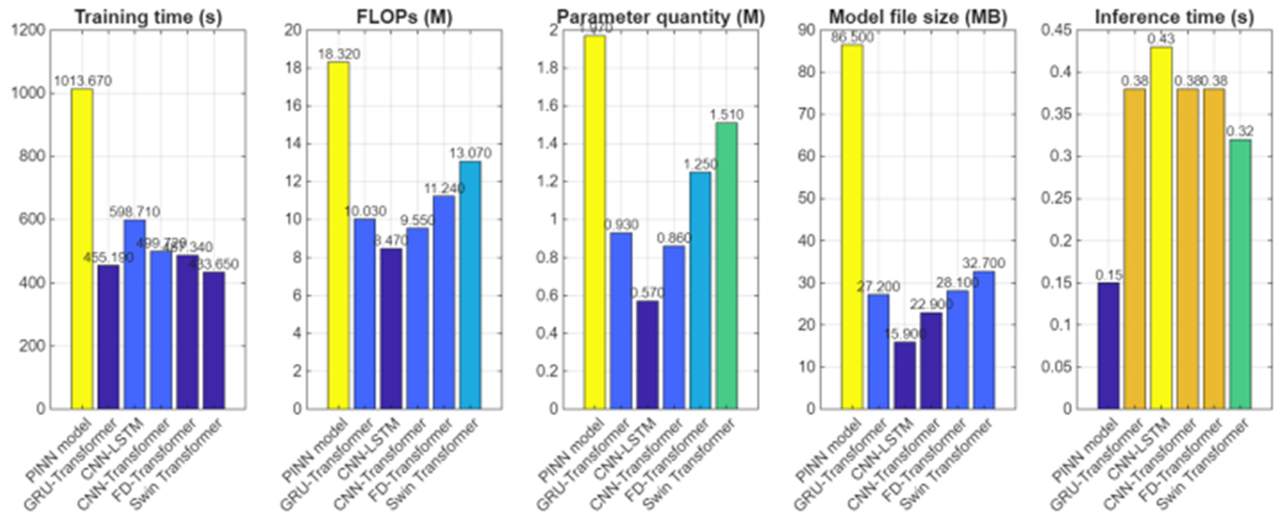
Table 5 provides a summary of the accuracy and precision metrics for each model (with accuracy expressed as mean ± standard deviation, and the coefficient of determination, root mean square error, and mean absolute percentage error all representing the average values from four training sessions). Figure 11 illustrates the inference and training times (averaged), FLOPs, parameter quantity, and file sizes (all measured in inference mode) for each model. As indicated in Table 5, the PINN model exhibits the highest mean fault identification accuracy and the lowest standard deviation. Concurrently, the coefficient of determination for crack length prediction is at a high level, while both the root mean square error and mean absolute percentage error are the lowest, demonstrating its superior damage identification capability, prediction accuracy, and stability compared to the other five comparative models. To further ascertain the statistical significance of this performance advantage, an independent samples t-test ($\alpha =0.05$) was performed, using the PINN model as the reference against the other models. The results reveal that the p-values between each comparative model and the PINN model are all approaching zero ($p<<0.001$), significantly below the significance threshold, thereby confirming the statistical reliability of the enhanced diagnostic accuracy of the PINN model.

Figure 11 visually displays the comparative results of six models concerning computing power-related metrics in the form of a heatmap. It is evident that the PINN method employed in this research surpasses the comparative models in terms of training time, model file size, parameter quantity, and FLOPs. Nevertheless, in practical engineering applications, it is customary to utilize high-performance computing platforms to accomplish the offline training and structural optimization of models using extensive historical samples. Subsequently, the fully trained model is solidified and deployed to an online monitoring system for swift identification and state assessment of real-time collected data, adhering to the engineering paradigm of “offline training + online inference”. Within this framework, inference time emerges as a pivotal metric for evaluating the model’s online performance. Experimental findings demonstrate that the method proposed in this paper exhibits the shortest inference time, further corroborating the merits of the PINN model: in contrast to purely data-driven deep networks, PINN effectively constrains the parameter search space and expedites the model optimization process by incorporating physical constraints into the loss function, thereby facilitating efficient learning and more stable convergence performance.

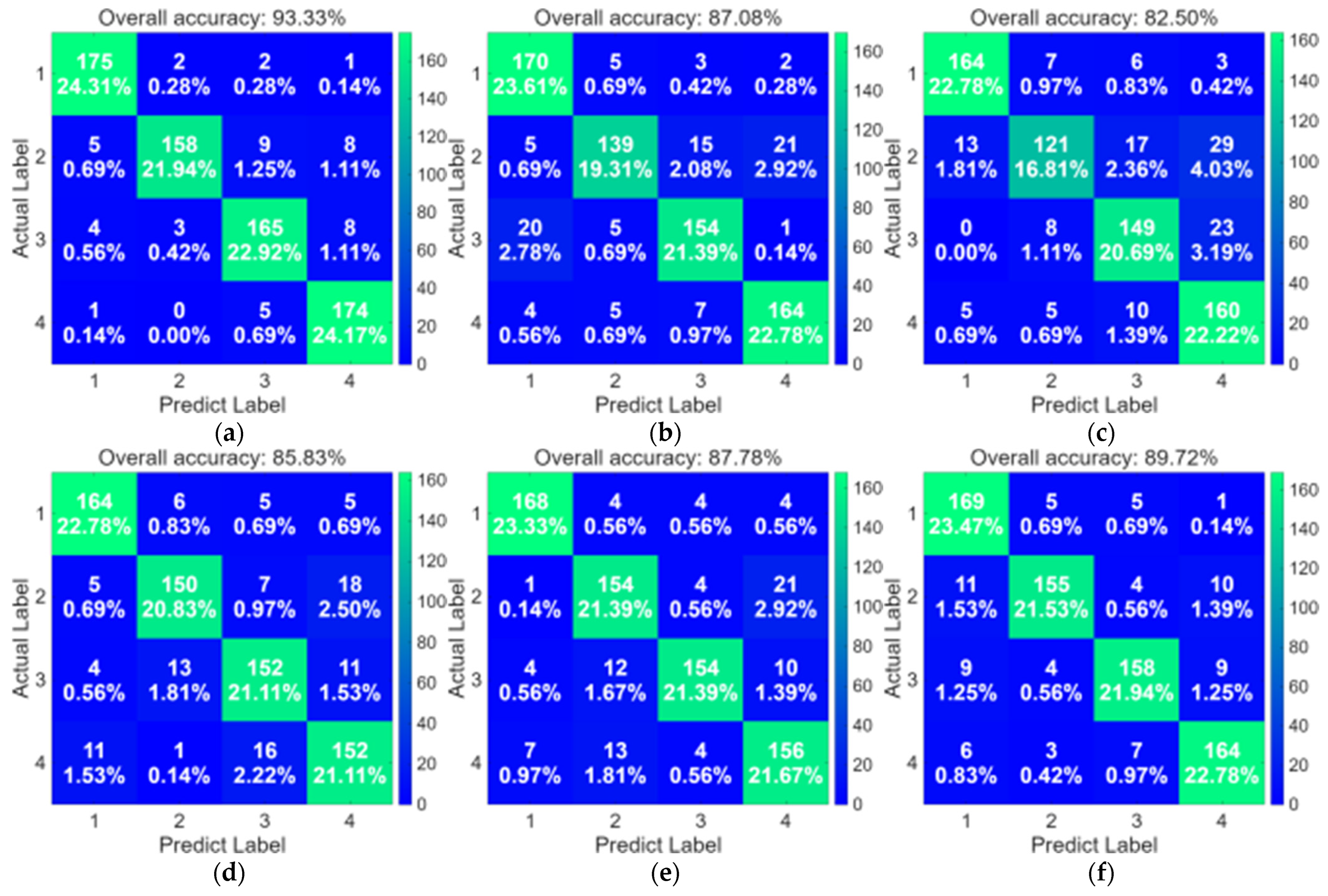
Figure 12 illustrates the optimal classification confusion matrices obtained from four independent experimental runs. Analysis of the figure indicates that each model demonstrates a relatively high recognition accuracy for fault mode F1. Nevertheless, when it comes to fault modes F2, F3, and F4, which involve cracks, there is a marked divergence in the recognition performance among the models. Specifically, comparative models, including GRU-Transformer, CNN-LSTM, CNN-Transformer, FD-Transformer, and Swin Transformer, generally exhibit limited recognition capabilities for the aforementioned types of crack damage, often leading to confusion between different crack patterns. This highlights the constraints of traditional data-driven models in effectively capturing crack-sensitive features. Conversely, the PINN model proposed in this study demonstrates robust recognition capabilities across all fault modes, significantly outperforming the comparative models in terms of classification accuracy and robustness. This suggests that incorporating physical information constraints into the model can substantially enhance its ability to extract and discriminate crack-induced vibration features.

4.2.2. Model Testing Based on Independent Datasets

Furthermore, to assess the generalization performance and engineering applicability of each model in real-world deployment scenarios, the model with the best accuracy and precision indicators was selected from the aforementioned four independent experiments for deployment. Subsequently, the chosen optimal models were subjected to application testing using the independent test sets outlined in Table 3, to validate their capability in identifying and localizing damage on unseen samples.

Table 6. Testing results of different models.

Model	Accuracy (%)	${\mathit{E}}_{{\mathit{R}}^2}$	${\mathit{E}}_{\mathit{R}\mathit{M}\mathit{S}\mathit{E}}$	${\mathit{E}}_{\mathit{M}\mathit{A}\mathit{P}\mathit{E}}$ (%)
PINN model	93.1	0.9284	1.8694	36.34
GRU-Transformer	86.94	0.8297	4.2715	47.28
CNN-LSTM	81.59	0.7128	5.835	56.14
CNN-Transformer	84.3	0.7589	5.2805	53.24
FD-Transformer	87.3	0.817	4.4755	48.04
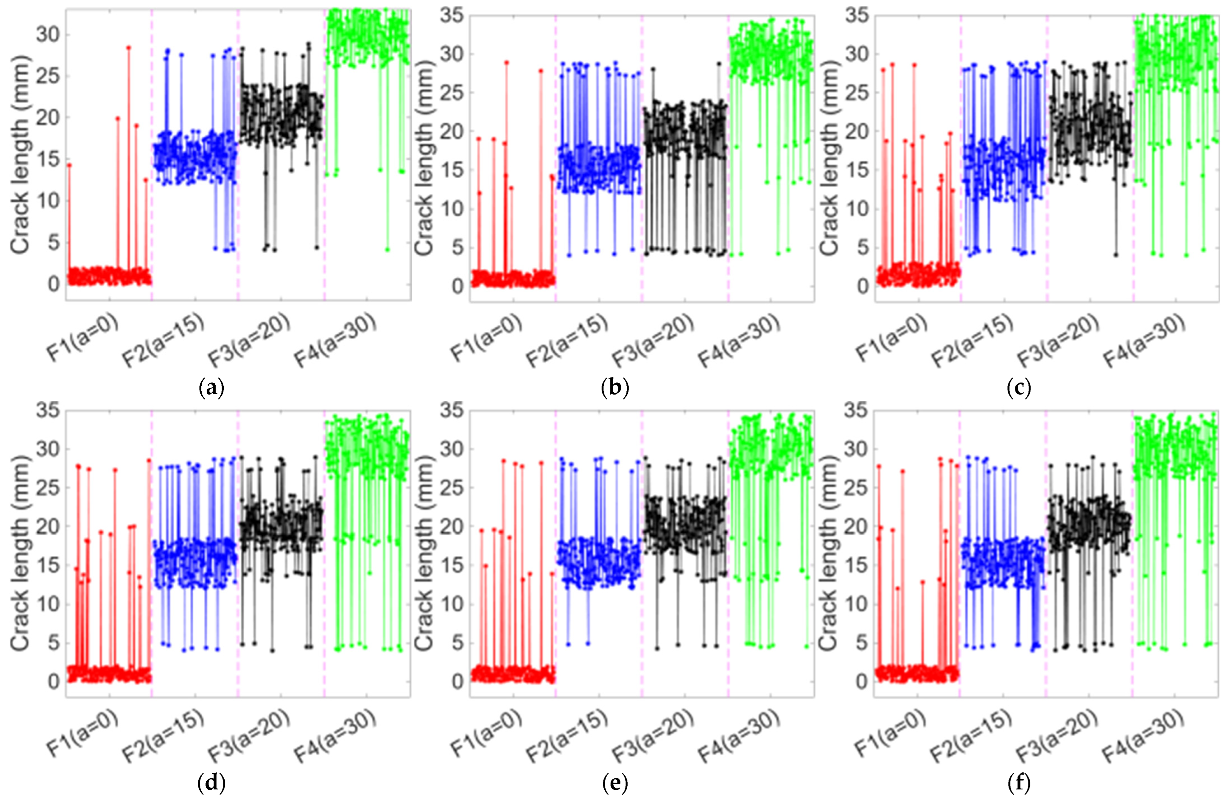
Swin Transformer	87.7	0.8231	4.3732	46.77

displays the testing outcomes of the aforementioned six models on an independent dataset, whereas Figure 13 and Figure 14 respectively depict the predictive results of each model concerning crack location $x_c$ and crack length $a$.

By analyzing Figure 13 and Table 6, it is evident that the PINN model proposed in this study demonstrates exceptional performance in predicting crack locations, achieving an overall accuracy exceeding 3%. This indicates that the PINN model exhibits high reliability in evaluating structural health conditions and effectively prevents false alarms. Furthermore, the model maintains a high recognition accuracy for various crack-related fault modes, thereby further confirming its superior performance and excellent engineering applicability in the task of crack localization in wind turbine blades. In contrast, other deep learning models, due to the absence of physical information constraints and excessively expansive hypothesis spaces, are prone to overfitting to noise rather than capturing true physical laws under conditions of limited sample sizes, consequently constraining their accuracy and generalization capabilities in fault diagnosis.

Further examination of Figure 14 and Table 6 demonstrates that, for the independent test set, the PINN model also demonstrates high precision in predicting crack length, boasting a notably superior coefficient of determination compared to other comparative models, with all error metrics remaining at a low level. This suggests that by explicitly incorporating physical conservation constraints into the loss function, a neural network that integrates physical information can adhere rigorously to the physical laws governing the relationship between cracks and vibrations, even under conditions of limited sample availability or significant measurement noise. Consequently, this ensures the stability and rationality of the prediction outcomes while effectively diminishing the model’s reliance on high-quality, voluminous training datasets. Conversely, traditional time-series prediction models lacking physical information constraints exhibit markedly inferior predictive performance relative to the method proposed in this research across all comparative approaches, particularly displaying substantial prediction discrepancies on datasets containing crack characteristics. The underlying reason is that traditional time-series prediction models rely exclusively on data-driven pattern recognition, rendering it challenging to capture the physical mechanisms underlying vibration disturbances caused by cracks. This results in pronounced deviations when extrapolating beyond the observed data distribution, thereby constraining their generalization capabilities. Hence, under conditions of limited sample size, traditional methods relying solely on data-driven approaches struggle to achieve high-quality identification and prediction of wind turbine blade damage.

4.3. Generalization Experiment

To further validate the generalization capability of the network, two rotational speed conditions unutilized during the training phase were introduced, namely 15 rpm and 25 rpm. Data under each of these two conditions was gathered for a duration of 2 min, yielding a total of 960 sample sets. Following an identical preprocessing protocol, the data was fed into the pre-trained network model for testing purposes. The results are presented in

Table 7. Result of generalization experiment (15 rpm).

Model	Accuracy (%)	${\mathit{E}}_{{\mathit{R}}^2}$	${\mathit{E}}_{\mathit{R}\mathit{M}\mathit{S}\mathit{E}}$	${\mathit{E}}_{\mathit{M}\mathit{A}\mathit{P}\mathit{E}}$ (%)
PINN model	92.83	0.9143	1.8933	37.92
GRU-Transformer	82.88	0.7939	4.3964	52.77
CNN-LSTM	66.34	0.6642	8.5240	60.96
CNN-Transformer	80.37	0.7303	5.6321	57.65
FD-Transformer	79.91	0.7738	4.6150	56.09
Swin Transformer	80.87	0.7929	4.9255	58.21

and

Table 8. Result of generalization experiment (25 rpm).

Model	Accuracy (%)	${\mathit{E}}_{{\mathit{R}}^2}$	${\mathit{E}}_{\mathit{R}\mathit{M}\mathit{S}\mathit{E}}$	${\mathit{E}}_{\mathit{M}\mathit{A}\mathit{P}\mathit{E}}$ (%)
PINN model	92.65	0.9110	1.902	38.66
GRU-Transformer	82.34	0.7891	4.6604	53.3
CNN-LSTM	67.22	0.6629	8.587	61.19
CNN-Transformer	79.82	0.7324	5.6939	58.46
FD-Transformer	79.15	0.7685	4.6521	55.74
Swin Transformer	81.22	0.7711	4.7769	57.4

. Through a comprehensive analysis of Table 7 and Table 8, it can be observed that under these two unfamiliar operating conditions, the fan blade damage identification model integrated with PINN still sustains high accuracy and prediction precision, showcasing robust generalization capabilities, whereas other networks experience a notable decline in performance.

4.4. Noise Resistance Experiment

To address the prevalent noise interference in engineering signals and validate the anti-noise capability of the method proposed in this paper, Gaussian white noise with a level of ±3 dB was introduced into the collected experimental data to simulate noisy operational conditions. Specifically, for the original signal denoted as $s(t)$, the noise-added signal is represented as $\tilde{s}\left(t\right)$, as follows:

$$\tilde{s}\left(t\right)=s\left(t\right)+\eta ·\sigma \left(s\right)·N\left(0,1\right)$$

(38)

where $\sigma \left(s\right)$ is the variance of the original signal, $N\left(0,1\right)$ denotes a standard Gaussian white noise sequence, and $\eta$ signifies the noise intensity coefficient. By setting $20 {\log }_{10}\left(\eta \right)=\pm 3\mathrm{dB}$, noise levels of ±3 dB can be introduced. To mitigate the incidental effects arising from a single realization of random noise, five independent sets of Gaussian white noise sequences are generated for each noise level. After injecting these sequences into the original signal, the mean of the model prediction results obtained from the five sets of noise-added signals corresponding to each sample is taken as the final prediction output for that sample. This approach helps to attenuate fluctuations in the evaluation metrics caused by the randomness inherent in individual noise instances.

The fault identification accuracy for noisy samples is detailed in

Table 9. Results of noise resistance experiment (−3 dB).

Model	Accuracy (%)	${\mathit{E}}_{{\mathit{R}}^2}$	${\mathit{E}}_{\mathit{R}\mathit{M}\mathit{S}\mathit{E}}$	${\mathit{E}}_{\mathit{M}\mathit{A}\mathit{P}\mathit{E}}$ (%)
PINN model	83.49	0.9168	1.8297	38.39
GRU-Transformer	69.52	0.7862	4.5591	55.28
CNN-LSTM	60.88	0.6271	9.5901	68.36
CNN-Transformer	67.50	0.7186	5.7559	59.51
FD-Transformer	67.56	0.7229	5.9111	61.53
Swin Transformer	73.46	0.7369	5.506	58.83

and

Table 10. Results of noise resistance experiment (3 dB).

Model	Accuracy (%)	${\mathit{E}}_{{\mathit{R}}^2}$	${\mathit{E}}_{\mathit{R}\mathit{M}\mathit{S}\mathit{E}}$	${\mathit{E}}_{\mathit{M}\mathit{A}\mathit{P}\mathit{E}}$
PINN model	83.23	0.91141	1.8288	38.75
GRU-Transformer	67.81	0.7681	4.7625	57.23
CNN-LSTM	63.1	0.6247	9.5926	67.89
CNN-Transformer	67.01	0.7155	5.7798	60.31
FD-Transformer	68.33	0.7301	5.8604	61.76
Swin Transformer	74.31	0.7366	5.6459	57.65

. The findings reveal that, under the two signal-to-noise ratio conditions examined, the proposed model exhibits superior accuracy and coefficient of determination compared to the other five benchmark models. Furthermore, it achieves the lowest levels of both root mean square error and mean absolute percentage error. These results comprehensively confirm that the proposed model preserves high precision in damage identification and localization even amidst substantial noise interference, thereby showcasing its remarkable noise resilience and robustness.

5. Conclusions and Prospects

To address the limitations inherent in data-driven vibration analysis methods, this research introduced a damage identification approach for wind turbine blades that integrates Physics-Informed Neural Networks (PINNs). Through crack damage simulation experiments, the correlation between crack damage and the three-dimensional vibration responses of the blade root bearing housing was analyzed. The following conclusions are drawn:

(1)

Compared to traditional deep network diagnostic methods, PINN can uncover latent data causal relationships within the “black box” structure, significantly enhancing the interpretability of the workflow and endowing the model with greater credibility and scalability.

(2)

The PINN-based damage identification model developed in this study surpasses traditional deep learning networks in terms of both inference speed and identification accuracy. Notably, under unfamiliar operating conditions and in environments with strong noise interference, it maintains high diagnostic accuracy, demonstrating superior physical consistency and generalization capabilities.

(3)

Compared to purely data-driven approaches, the model incorporating physical information exhibits significantly superior performance across various evaluation metrics. The robustness conferred by physical constraints not only enhances model performance but also refines its underlying mechanisms, thereby providing more reliable technical support for elevating the intelligence level of wind turbine operation and maintenance and ensuring the long-term safe and stable operation of wind turbines.

Meanwhile, the research content presented in this manuscript exhibits certain limitations. During the construction of the crack-vibration physical information constraint model, complex rotor dynamics equations were necessarily simplified, taking into account real-time computation and model convergence requirements. Specifically, wind turbine blades were modeled as rotating cantilever Euler–Bernoulli beams, disregarding the influences of shear deformation, rotational inertia, and nonlinear aerodynamic damping. Additionally, an ideal torsional spring model was employed to characterize crack features, with modeling predicated on the assumptions of single-mode dominance and small crack perturbation. However, the actual engineering environment is considerably more intricate than the simplified model. Blades are subjected to wind load excitations that vary both spatially and temporally, encountering complex boundary conditions such as tower shadow effects and blade-hub coupling, while also being influenced by material nonlinearity, temperature effects, and nonlinear contact stiffness arising from bolt connections. Furthermore, the fluid–structure interaction between airflow and the structure induces nonlinear variations in added mass and aerodynamic damping, whereas the crack breathing effect introduces time-varying characteristics to system stiffness, thereby eliciting rich superharmonic and subharmonic response components. These nonlinear and time-varying factors result in real vibration signals often encompassing complex modulation characteristics and broadband responses, which significantly surpass the descriptive capacity of the simplified physical model. Additionally, constrained by experimental conditions and costs, the current experimental dataset encompasses only four typical crack scenarios. The variations in crack location and length have not been fully independently combined, and the sample size remains relatively small. Additionally, all experimental data are derived from the same test rig and the same blade model, with no cross-validation performed across different blade specimens or test rigs. This, to a certain extent, limits the comprehensive validation of the model’s generalization capability and the statistical robustness of the conclusions drawn.

Notwithstanding the aforementioned limitations, this research nonetheless offers novel theoretical insights and technical underpinnings for the damage detection and fault diagnosis of wind turbine blades. Subsequent research endeavors will be directed towards incorporating a broader array of practical considerations to further refine the physically informed constraint model.

References

1. Chen, X.-F.; Guo, Y.-J.; Xu, C.-B.; Shang, H.-B. Review of fault diagnosis and health monitoring for wind power equipment. China Mech. Eng. 2020, 31, 175–189. [Google Scholar] [CrossRef]
2. Zhang, D.-H.; Wang, Y.-M.; Jiang, Y.-J.; Zhao, T.; Xu, H.-Y.; Qian, P.; Li, C.-L. A novel Wind Turbine Rolling Element Bearing Fault Diagnosis Method Based on CEEMDAN and Improved TFR Demodulation Analysis. Energies 2024, 17, 819. [Google Scholar] [CrossRef] [Scilit]
3. Wang, S.; Vidal, Y.; Pozo, F. Recent advances in wind turbine condition monitoring using SCADA data: A state-of-the-art review. Reliab. Eng. Syst. Saf. 2026, 267, 111838. [Google Scholar] [CrossRef] [Scilit]
4. Data Source: OCPE. Available online: http://www.ocpe.com.cn (accessed on 20 March 2026).
5. Analysis of the Manifestations, Diagnosis, and Maintenance Points of Wind Turbine System Faults. Available online: https://www.in-en.com/article/html/energy-2265000.shtml (accessed on 20 March 2026).
6. Chen, N.; Zhao, Z.; Lin, L. A hybrid deep learning method for AE source localization for hetero-structure of wind turbine blades. Mar. Struct. 2024, 94, 03562. [Google Scholar] [CrossRef] [Scilit]
7. Ogaili, A.; Jaber, A.; Hamzah, M. A methodological approach for detecting multiple faults in wind turbine blades based on vibration signals and machine learning. Curved Layer. Struct. 2023, 10, 20220214. [Google Scholar] [CrossRef] [Scilit]
8. Wang, C.; Gu, Y. Research on infrared nondestructive detection of small wind turbine blades. Results Eng. 2022, 15, 100570. [Google Scholar] [CrossRef] [Scilit]
9. Kaewniam, P.; Cao, M.; Alkayem, N. Recent advances in damages detection of wind turbine blades: A state-of-the-art review. Renew. Sustain. Energy Rev. 2022, 167, 112723. [Google Scholar] [CrossRef] [Scilit]
10. Deng, L.W.; Guo, Y.G.; Chai, B.R. Defect detection on a wind turbine blade based on digital image processing. Processes 2021, 9, 1452. [Google Scholar] [CrossRef] [Scilit]
11. Memari, M.; Skakya, P.; Shekaramiz, M. Review on the advancements in wind turbine blade inspection: Integrating drone and deep learning technologies for enhanced defect detection. IEEE Access 2024, 12, 33236–33282. [Google Scholar] [CrossRef] [Scilit]
12. Chen, B.; Yu, S.; Yu, Y. Acoustical damage detection of wind turbine blade using the improved incremental support vector data description. Renew. Energy 2020, 156, 548–557. [Google Scholar] [CrossRef] [Scilit]
13. Chen, B.; Zhang, M.; Lin, Z. Acoustic-based whistle detection of drain hole for wind turbine blade. ISA Trans. 2022, 131, 736–747. [Google Scholar] [CrossRef] [Scilit] [PubMed]
14. García, D.; Tcherniak, D. An Experimental study on the data-driven structural health monitoring of large wind turbine blades using a single accelerometer and actuator. Mech. Syst. Signal Process. 2019, 127, 102–119. [Google Scholar] [CrossRef] [Scilit]
15. Joshuva, A.; Kumar, R.; Sivakumar, S. An insight on VMD for diagnosing wind turbine blade faults using C4.5 as feature selection and discriminating through multilayer perception. Alex. Eng. J. 2020, 59, 3863–3879. [Google Scholar] [CrossRef] [Scilit]
16. Fremmelev, M.A.; Ladpli, P.; Orlowitz, E.; Dervilis, N.; McGugan, M.; Branner, K. A full-scale wind turbine blade monitoring campaign: Detection of damage initiation and progression using medium-frequency active vibrations. Struct. Health Monit. 2023, 22, 4171–4193. [Google Scholar] [CrossRef] [Scilit]
17. Andeas, P.; Tcherniak, D.; Fassois, D.S. Damage detection on the blade of an operating wind turbine via a single vibration sensor and statistical time series methods: Exploring the performance limits of robust methods. Struct. Health Monit. 2023, 22, 1475–9217. [Google Scholar] [CrossRef] [Scilit]
18. Wang, M.; Zhang, X.-F.; Qin, G.J.; Liu, M. Wind turbine blade fault diagnosis integrating multi-scale enhanced hierarchical fuzzy entropy, isolation forest and GWO-GRU. Entropy 2026, 28, 810. [Google Scholar] [CrossRef] [Scilit]
19. Ayankoso, S.; Dutta, A.; He, Y.-H.; Gu, F.S.; Bal, A.; Pa, S.K. Performance of vibration and current signals in the fault diagnosis of induction motors using deep learning and machine learning techniques. Struct. Health Monit. 2026, 25, 196–212. [Google Scholar] [CrossRef] [Scilit]
20. Gómez, M.C.; García-Vellisca, M.A.; Do-Cabo, C.T.; Xi, Y.J.; Mao, Z. Structural health monitoring through deep learning: A study on scalogram-based vibration signal classification. J. Low Freq. Noise Vib. Act. Control. 2026, 45, 404–419. [Google Scholar] [CrossRef] [Scilit]
21. Sarma, I.V.; Chanda, S.; Reddy, M.S. Interpretable ai for vibration-based structural health monitoring: A comparative study of CNN and Transformer architectures on a benchmark shear building. Asian J. Civ. Eng. 2026, 26, 4615–4628. [Google Scholar] [CrossRef] [Scilit]
22. Zhang, X.-L.; Zhou, W.-S. Structural vibration data anomaly detection based on multiple feature information using CNN-LSTM model. Struct. Control Health Monit. 2023, 2023, 3906180. [Google Scholar] [CrossRef] [Scilit]
23. Wei, H.; Jian, X. A proposed recursive TCN–GRU for the time-series forecast of engineering vibration. J. Vib. Acoust. 2025, 147, 061008. [Google Scholar] [CrossRef] [Scilit]
24. Yao, Z.-Q.; Wu, M.; Qian, J.; Reynaerts, D. Non-invasive radio frequency (RF)-driven in-process monitoring and control for enhancing micro-electrical discharge machining stability and efficiency. Mech. Syst. Signal Process. 2026, 249, 114072. [Google Scholar] [CrossRef] [Scilit]
25. Khan, M.A.; Munir, S.; Ali, M.N.; Kim, B.S. Deep learning based smart energy consumption prediction in residential buildings. PeerJ Comput. Sci. 2026, 12, e3689. [Google Scholar] [CrossRef] [Scilit]
26. Alizamir, M.; Ahmed, K.O.; Heddam, S.; Kim, S.; Lee, J.E. Daily soil temperature prediction using hybrid deep learning and SHAP for sustainable soil management. Eng. Appl. Comput. Fluid Mech. 2025, 19, 2541686. [Google Scholar] [CrossRef] [Scilit]
27. Liu, S.-Y.; Wang, C.-H.; Sun, X.-H.; Yang, Z.-B.; Ma, Z.-Q. Graph neural network based on multi-source and multi-feature nodes for fault diagnosis of bearings under variable rotating speed working condition. J. Vib. Shock 2026, 3, 201–209. [Google Scholar] [CrossRef]
28. Zhao, Y.; Zhang, Y.; Li, Z. AI-enabled and multimodal data driven smart health monitoring of wind power systems: A case study. Adv. Eng. Inform. 2023, 56, 102018. [Google Scholar] [CrossRef] [Scilit]
29. Zhou, Q.-Z.; Mu, Y.; Wu, H.-N.; Chen, X.; Wang, F.; Li, C.; Zhang, W.; Liu, P.-P.; Wang, C. Fault detection and classification of wind turbine blades based on machine learning. J. Jilin Univ. Eng. Technol. Ed. 2025, 55, 3119–3130. [Google Scholar] [CrossRef]
30. Wang, M.-H.; Lu, S.-D.; Hsieh, C.C. Fault detection of wind turbine blades using multi-channel CNN. Sustainability 2022, 14, 1781. [Google Scholar] [CrossRef] [Scilit]
31. Pałczyński, C.; Olejnik, P. Anomalies classification in fan systems using dual-branch neural networks with continuous wavelet transform layers: An experimental study. Information 2025, 16, 71. [Google Scholar] [CrossRef] [Scilit]
32. Sethi, M.; Subba, A.; Faisal, M. Fault diagnosis of wind turbine blades with continuous wavelet transform based deep learning model using vibration signal. Eng. Appl. Artif. Intell. 2024, 138, 109372. [Google Scholar] [CrossRef] [Scilit]
33. Raissi, M.; Perdikaris, P.; Karniadaks, G.E. Physic informed deep learning: A deep learning framework for solving forward and inverse problems involving nonlinear partial differential equations. J. Comput. Phys. 2018, 378, 686. [Google Scholar] [CrossRef] [Scilit]
34. Zhang, Y.; Liu, P.; Liu, Q.-C. Method for predicting the high-cycle fatigue remaining useful life of aero-engine blades based on physics-informed neural networks. J. Vib. Eng. 2025, 38, 1190–1198. [Google Scholar] [CrossRef]
35. Panagiotopoulou, V.; Vlachas, K.; Giglio, M. Damage identification in rotary shafts via vibration monitoring and physics-informed neural networks. In Proceedings of the 11th International Operational Modal Analysis Conference, Rennes, France, 20–23 May 2025. [Google Scholar]
36. Yucesan, Y.A.; Viana, F.A. A hybrid physics-informed neural network for main bearing fatigue prognosis under grease quality variation. Mech. Syst. Signal Process. 2022, 33, 108875. [Google Scholar] [CrossRef] [Scilit]
37. Liu, X.; Cheng, W.; Xing, J.; Chen, X.-F.; Zhao, Z.-B.; Zhang, R.-Y.; Huang, Q.; Lu, J.-L.; Zhou, H.-P.; Zheng, W.-X.; et al. Physics-informed Neural Network for system identification of rotors. IFAC-PapersOnLine 2024, 58, 307–312. [Google Scholar] [CrossRef] [Scilit]
38. Wang, F.-J.; Zhai, Z.; Zhao, Z.-B.; Di, Y.; Chen, X.-F. Physics-informed neural network for lithium-ion battery degradation stable modeling and prognosis. Nat. Commun. 2024, 15, 4332. [Google Scholar] [CrossRef] [Scilit] [PubMed]
39. Wang, M.; Qin, G.J.; Liu, M. Electrochemical response characteristics during the oxidative degradation of gear oil in wind turbine generators. Lubricants 2026, 14, 272. [Google Scholar] [CrossRef] [Scilit]
40. Jo, J.Y.; Jeong, Y.; Kim, J.; Yoo, J. Thermal conductivity estimation using physics-informed neural networks with limited data. Eng. Appl. Artif. Intell. 2024, 137, 109079. [Google Scholar] [CrossRef] [Scilit]
41. Sun, H.-D.; He, H.-X.; Cheng, Y. Experimental study on the mechanical mechanism and vibration reduction performance of suspended multi-mass pendulums. J. Vib. Shock 2024, 43, 50–63. [Google Scholar] [CrossRef]
42. Yang, Y.-K.; Wang, X.-F.; Li, J.-F.; Ge, R. A data-physic driven method for gear fault diagnosis using PINN and pseudo-dynamic features. Meas. J. Int. Meas. Confed. 2024, 236, 115124. [Google Scholar] [CrossRef] [Scilit]
43. Shakya, P.; Sunny, M.R.; Maiti, D.K. Time domain flutter analysis of bend-twist coupled large composite wind turbine blades: A parametric study. Mech. Based Des. Struct. Mach. 2020, 50, 4048–4070. [Google Scholar] [CrossRef] [Scilit]
44. Shao, B.; Fan, C.-G.; Fu, S.-G.; Zeng, J. Analysis of the nonlinear complex response of cracked blades at variable rotational speeds. Machines 2024, 12, 725. [Google Scholar] [CrossRef] [Scilit]
45. Wolniak, M.; Ragnitz, J.; Jonscher, C.; Hofmeister, B.; Jauken, H.; Hübler, C.; Rolfes, R. Damage identification on a large-scale wind turbine rotor blade using sample-based deterministic model updating. Wind Energy Sci. 2026, 11, 1227–1249. [Google Scholar] [CrossRef] [Scilit]
46. Li, X.-J.; Diao, Y.-S.; Lü, J.-D.; Hou, J.-R. Damage Identification of An Offshore Wind Turbine Supporting Structure Based on A CNN-GRU Parallel Network. J. Vib. Shock 2024, 43, 229–237. [Google Scholar] [CrossRef]
47. Li, Y.-H.; Zhang, Y.; Yang, T.-J.; Shi, R.-B. Remaining useful life prediction of rolling bearings based on MRF-GCN-Transformer. J. Vib. Shock 2025, 44, 328–337. [Google Scholar] [CrossRef]
48. Lasfar, R.; Toth, G. The difference of model robustness assessment using cross-validation and bootstrap methods. J. Chemom. 2024, 38, e3530. [Google Scholar] [CrossRef] [Scilit]
49. Wang, S.-F.; Teng, Y.-J.; Perdikaris, P. Understanding and mitigating gradient flow pathologies in physics-informed neural networks. SIAM J. Sci. Comput. 2021, 43, A3055–A3081. [Google Scholar] [CrossRef] [Scilit]
50. Dong, M.; Chen, J.; Chang, H.-X.; Hu, Y.-Z.; Zhang, C.-X.; Zhang, H.-B.; Dong, X. Research on prediction method of dissolved gas in transformer oil based on physical information neural network model. Electr. Mach. Control. 2025, 29, 1–12. [Google Scholar] [CrossRef]
51. Xiang, L.; Wang, P.-H.; Li, J.-X. Abnormal state detection of wind turbines based on CNN-LSTM. J. Vib. Shock 2021, 40, 11–17. [Google Scholar] [CrossRef]
52. Sheng, R.; Xu, J.-S.; Wei, B.-T.; Wang, B. Diagnosis of intake and exhaust faults in aviation piston engine based on CNN-Transformer interactive fusion network. J. Vib. Shock 2025, 44, 258–269. [Google Scholar] [CrossRef]
53. Zhao, Z.-H.; Li, C.-X.; Li, L.-H.; Yang, S.-P. A FD-Transformer method for fault diagnosis of mechanical equipment. J. Vib. Shock 2023, 42, 326–333. [Google Scholar] [CrossRef]
54. Chen, Z.-G.; Tao, Z.-C.; Wang, Y.-X.; Wei, Z.-S. Fault diagnosis method of planetary gearbox with TCN-Transformer based on hybrid attention mechanism. J. Vib. Shock 2025, 44, 348–356. [Google Scholar] [CrossRef]
Figure 1. Simulation experiment setup for wind turbine blade failure. (a) Double-fed wind turbine scaled-down test bench; (b) three-directional vibration sensor.
Machines 14 00857 g001
Figure 2. Image of prefabricated fault components. (a) F2; (b) F3; (c) F4.
Machines 14 00857 g002
Figure 3. Vibration spectrum in X-direction. (a) F1; (b) F2; (c) F3; (d) F4.
Machines 14 00857 g003
Figure 4. Vibration spectrum in Y-direction. (a) F1; (b) F2; (c) F3; (d) F4.
Machines 14 00857 g004
Figure 5. Vibration spectrum in Z-direction. (a) F1; (b) F2; (c) F3; (d) F4.
Machines 14 00857 g005
Figure 6. A schematic diagram of a rotating cantilever Euler–Bernoulli beam structure.
Machines 14 00857 g006
Figure 7. Schematic diagram of GRU-Transformer network.
Machines 14 00857 g007
Figure 8. Structure diagram of GRU neuron.
Machines 14 00857 g008
Figure 9. Flowchart of multi-head self-attention mechanism.
Machines 14 00857 g009
Figure 10. Structural diagram of blade damage recognition model.
Machines 14 00857 g010
Figure 11. Heat map of computational metrics.
Machines 14 00857 g011
Figure 12. Classification confusion matrix. (a) PINN model; (b) GRU-Transformer; (c) CNN-LSTM; (d) CNN-Transformer; (e) FD-Transformer; (f) Swin Transformer.
Machines 14 00857 g012
Figure 13. Prediction results of crack locations by different models. (a) PINN model; (b) GRU-Transformer; (c) CNN-LSTM; (d) CNN-Transformer; (e) FD-Transformer; (f) Swin Transformer.
Machines 14 00857 g013
Figure 14. Prediction results of crack length by different models. (a) PINN model; (b) GRU-Transformer; (c) CNN-LSTM; (d) CNN-Transformer; (e) FD-Transformer; (f) Swin Transformer.
Machines 14 00857 g014