Numerical Investigation on the Relationship Between Pitch Angle Variance and Milling Stability with Waveform Parameter Variations

Abstract

Wave-edge milling tools can suppress chatter by introducing periodic harmonic variations along the cutting edge, which change the tooth-passing time delays between adjacent teeth. However, their stability is affected by coupled waveform parameters, such as amplitude, wavelength, and phase, making it difficult to screen suitable parameter combinations efficiently. This numerical/modeling-based study uses a previously validated multi-delay dynamic model to investigate the probabilistic relationship between pitch angle variance (PAV) and stability region area (SRA). A large number of feasible waveform-parameter combinations are generated under geometric constraints, and a PAV-based stratified sampling strategy is used to retain 54 representative parameter sets from six PAV layers for stability lobe diagram construction and SRA calculation. The results show that PAV has weak pointwise predictive capability for individual SRA values, with Pearson = 0.4234, Spearman = 0.4720, and R² = 0.179. However, the stratified statistical results reveal a clear layer-wise probabilistic tendency: the mean SRA increases from 17.962 to 20.996 in units of rpm·m, and the probability of obtaining an above-median SRA increases from 11.1% to 88.9%. The high-value tail case with PAV > 0.06 further indicates that a higher PAV does not necessarily guarantee a larger SRA for an individual parameter set. Therefore, PAV should not be used as a deterministic predictor or stand-alone tool-selection criterion, but can serve as a low-cost auxiliary probabilistic pre-screening descriptor before high-fidelity SLD/SRA evaluation.

1. Introduction

Wave-edge milling tools suppress regenerative chatter by reconstructing the cutting-edge geometry and introducing non-uniform tooth-passing time delays. Their stability performance is governed not only by the wave-edge structure itself, but also by the coupled configuration of waveform parameters such as amplitude, wavelength, and phase. These coupled variations can simultaneously change local helix angles, pitch-angle distributions, and inter-tooth time delays, leading to more complex multi-delay dynamic behavior. Consequently, constructing stability lobe diagrams and calculating the stability region area for all feasible parameter combinations would result in a high computational cost. Therefore, a low-cost pre-screening strategy based on time-delay diversity is needed to narrow the candidate waveform-parameter space before high-fidelity stability evaluation.

Existing studies on chatter suppression by altering inter-tooth phase relationships and regenerative time delays first focused on unequal-pitch and variable-pitch milling tools. Sellmeier and Denkena [1] pointed out that unequal-pitch milling tools transform the single-delay problem in conventional milling into a multi-delay system and may generate stability islands in the stable domain. Suzuki et al. [2] proposed a robust unequal-pitch design method based on the regeneration factor. Stepan et al. [3] discussed the ultimate chatter-suppression capability of variable-pitch tools. Mei et al. [4] further established an analytical design model for alternating variable-pitch tools and validated it experimentally. On this basis, related studies were extended to variable-helix tools and combined variable-pitch–variable-helix tools. Comak and Budak [5] established the corresponding geometric, dynamic, and stability analysis framework. Zhan et al. [6] extended this concept to five-axis ball-end milling cutters. Niu et al. [7] indicated that the runout effect can significantly influence the chatter-suppression performance of variable-pitch and variable-helix tools. Otto et al. [8] emphasized that such tools correspond to periodic time-varying systems with multiple or distributed time delays. Yusoff and Sims [9] improved the chatter stability of variable-helix tools from the perspective of optimization design. Guo et al. [10] proposed an optimization method for variable-helix tools targeting the absolutely stable region and introduced a suppression factor to quantify chatter-suppression capability. For difficult-to-machine materials, Li et al. [11] applied variable-pitch design to the milling of Ti-6Al-4V, analyzed the influence of time-delay perturbations on the system instability factor using the Routh criterion, and validated the specially designed variable-pitch tool through simulations and experiments. In addition, Nie et al. [12,13] analyzed the vibration-reduction mechanism and stability prediction of variable-pitch milling tools from the perspectives of time–frequency characteristics and multiple time delays. Ozsahin [14] optimized variable-pitch tools by maximizing the chatter-free axial depth of cut, while Hu et al. [15] showed that non-constant helix structures can improve machining stability by modifying local inter-tooth phase relationships and time delays. In addition to conventional variable-pitch and variable-helix cutters, recent studies have further shown that special edge geometries and anti-vibration tool structures can modify the regenerative mechanism and improve chatter stability. Sims et al. [16] developed stability prediction methods for variable-pitch and variable-helix milling tools, while Jiang et al. [17] considered axially varying dynamics and cutter runout effects in variable-pitch/helix milling systems. Tehranizadeh et al. [18] experimentally compared special end mills for thin-walled part machining, and Yang et al. [19] demonstrated that damping-enhanced tool structures can significantly increase milling stability.

However, most existing studies on variable-pitch, variable-helix, serrated, and wave-edge tools focus on either directly prescribed pitch/helix distributions or separated investigations of predefined waveform parameters. In variable-pitch and variable-helix tools, the non-uniform tooth spacing or helix distribution is usually treated as the direct design variable, whereas in wave-edge milling tools the pitch-angle and time-delay diversity are generated indirectly by coupled waveform parameters, including amplitude, wavelength, and phase. Previous studies on serrated or wave-edge tools have provided important modeling and stability-prediction frameworks, but they mainly examined individual waveform parameters or specific edge profiles. Jiang et al. [20] further established an explicit geometric and multi-delay dynamic model for wave-edge milling tools and introduced PAV to characterize time-delay diversity. Nevertheless, whether PAV can be extended from a post-analysis descriptor to a practical pre-screening tool in a large-scale coupled waveform-parameter space has not been systematically examined. Therefore, the methodological difference of the present study lies not in proposing a new dynamic model or a new PAV index, but in evaluating the limited probabilistic screening capability and applicability boundary of PAV before high-fidelity SLD/SRA calculation.

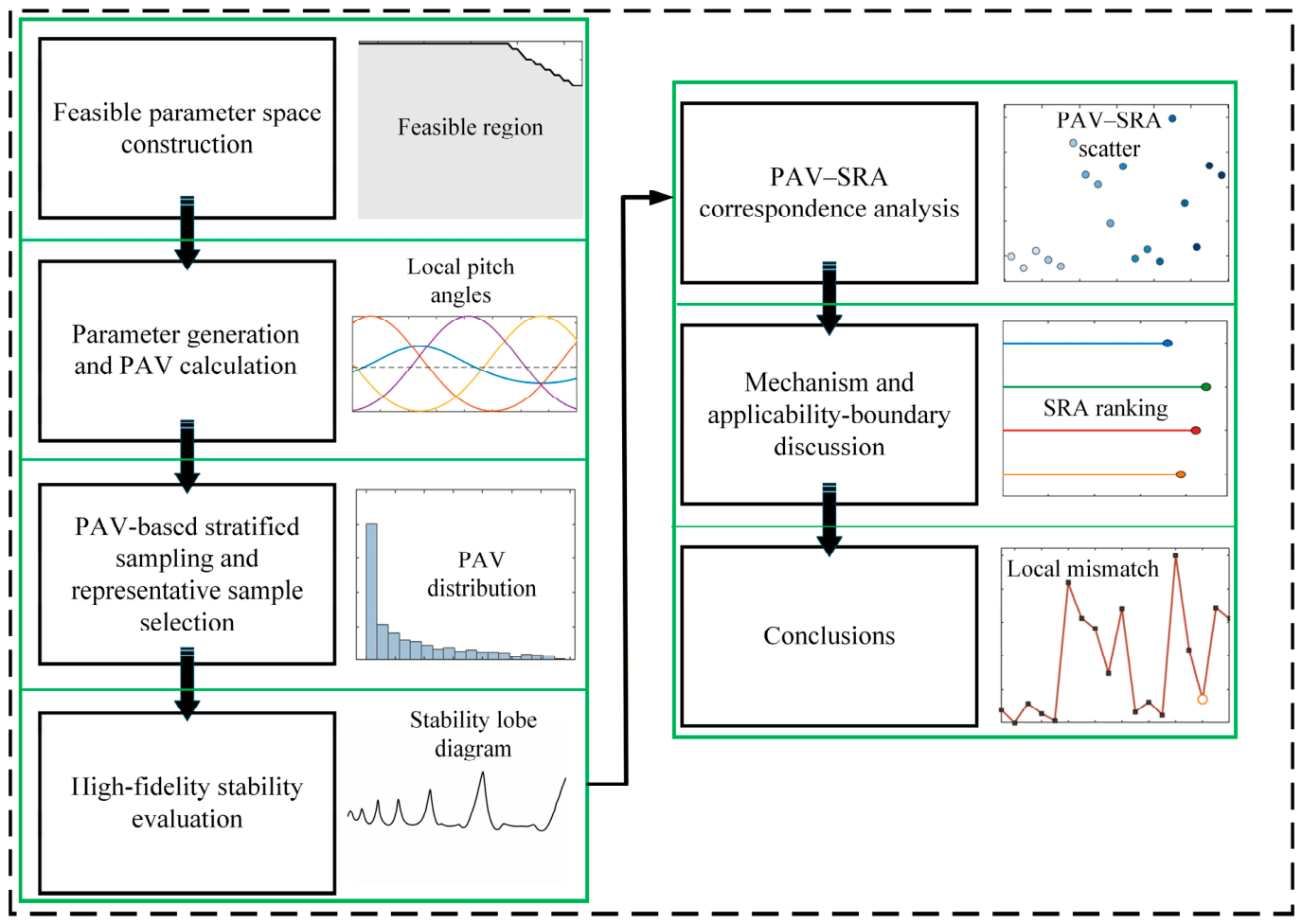
Therefore, based on the geometric model, dynamic model, and PAV-based characterization concept for wave-edge milling tools established by Jiang et al. [20], this study further focuses on a more design-oriented problem: how to rapidly identify candidate parameter configurations with superior stability at a relatively low computational cost when amplitude, wavelength, and phase vary cooperatively in a large-scale parameter space. To this end, on the basis of the existing modeling framework for wave-edge milling tools, a PAV-based stratified sampling strategy is introduced to examine whether PAV can provide probability-biased pre-screening information for waveform parameters before high-fidelity stability evaluation. The overall workflow of the proposed PAV-based probability-biased pre-screening and SLD/SRA-based stability evaluation framework is illustrated in Figure 1.

The main contributions of this study are: (1) constructing a feasible coupled waveform-parameter space involving amplitude, wavelength, and normalized phase ratio; (2) proposing a PAV-based stratified sampling strategy to reduce the number of high-fidelity SLD/SRA calculations from 2000 candidate combinations to 54 representative samples; (3) distinguishing the weak pointwise predictive capability of PAV from its layer-wise probability-biased screening capability; and (4) clarifying the applicability boundary of PAV, namely that it cannot deterministically predict the SRA of each individual parameter set but is associated with a higher observed probability of identifying large-SRA candidate regions. The research gap addressed is whether PAV can provide a probability-biased pre-screening basis in a large-scale coupled waveform-parameter space, rather than whether it can deterministically predict the SRA of each individual parameter set.

The remainder of this paper is organized as follows. Section 2 introduces the geometric modeling framework and the PAV-based characterization of time-delay diversity for wave-edge milling tools. Section 3 presents the construction of the feasible waveform-parameter space and the PAV-based stratified sampling strategy. Section 4 describes the stability prediction method and the definition of SRA. Section 5 analyzes the pointwise and stratified probabilistic relationship between PAV and SRA, discusses the applicability boundary of PAV as a probability-biased pre-screening descriptor, and compares typical stability lobe diagrams. Section 6 summarizes the main conclusions and future work.

2. Wave-Edge Milling Modeling and PAV-Based Characterization of Time-Delay Characteristics

2.1. Geometric Description of the Wave-Edge Milling Tool

The geometric description used in this section follows the explicit parametric modeling framework for wave-edge milling tools proposed by Jiang et al. [20]. This model is adopted as the theoretical basis of the present study rather than introduced as a new model.

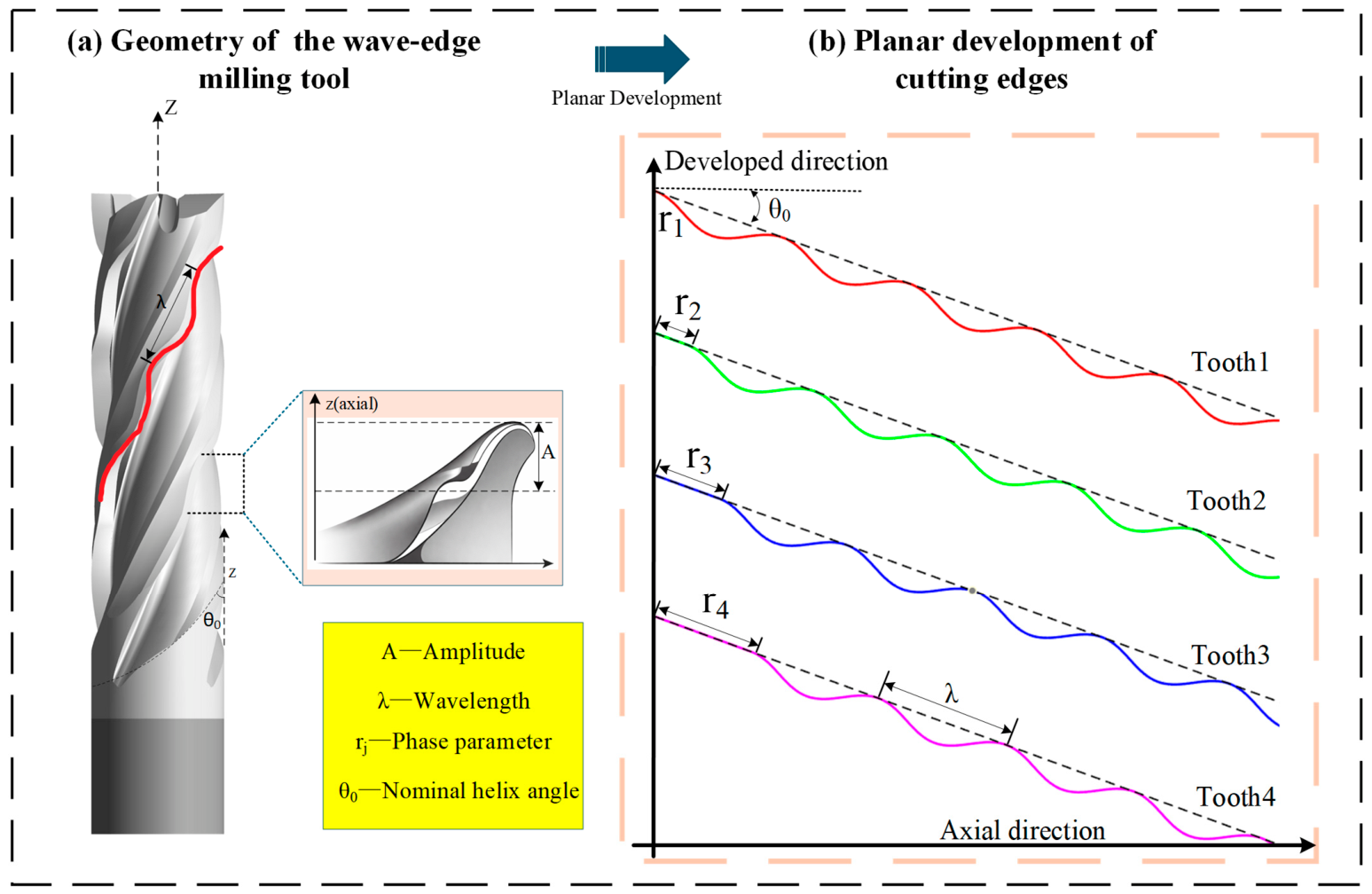
As shown in Figure 2, to facilitate the description of the geometric configuration of the wave-edge milling tool and the waveform differences among different teeth, the three-dimensional geometric schematic of the wave-edge milling tool and the planar development diagram of the cutting edges are presented, respectively. Figure 2a shows the overall structural characteristics of the wave-edge milling tool, in which the cutting edges exhibit continuous harmonic undulations along the tool axis. Its geometric morphology is jointly determined by the amplitude $A_j$, wavelength ${\lambda }_j$, and nominal helix angle ${\theta }_{0j}$. The locally enlarged view further illustrates the undulating characteristics of a single wave-edge profile. Figure 2b presents the planar development form of the cutting edges of a four-tooth wave-edge milling tool. When the position variable in the developed coordinate system is smaller than the phase parameter $r_j$, the profile remains a reference straight line; when it exceeds $r_j$, the cutting-edge profile varies according to a harmonic function.

Under the explicit parametric framework, the waveform profile of the j-th tooth can be expressed as a piecewise harmonic function. The amplitude $A_j$ determines the undulation magnitude of the cutting-edge waveform, the wavelength ${\lambda }_j$ determines the variation period of the waveform along the axial direction, and the phase parameter $r_j$ controls the relative waveform position among different teeth. Accordingly, only the basic expression required for the subsequent analysis is retained as follows:

$$y_{0j}=\left(\begin{array}{cc}0,\hfill & \hfill x_{0j}<r_j\\ A_j\sin (a_j{x}_{0j}+b_j)+A_j,\hfill & x_{0j}>r_j\hfill \end{array}\right.$$

(1)

where

$$\begin{array}{l}{a}_j={\displaystyle \frac{2\pi }{{\lambda }_j}}\\ b_j=-{\displaystyle \frac{\pi }{2}}-r_j{a}_j\end{array}$$

(2)

where $a_j$ is the angular wavenumber of the harmonic edge profile of the j-th tooth, and $b_j$ is the phase-offset coefficient determined by $a_j$ and the phase parameter $r_j$.

2.2. Non-Uniform Inter-Tooth Time Delays Induced by Waveform Variations

After the planar developed profile of each tooth is obtained, the cutting-edge positions corresponding to different axial discrete layers in three-dimensional space can be further determined through rotation, discretization, and interpolation by incorporating the nominal helix angle ${\theta }_{0j}$ and nominal pitch distance $L_{0j}$. To facilitate the subsequent time-delay analysis, the lag distance of the j-th tooth at the k-th axial discrete layer relative to its standard line is defined as $d_{k,j}$, which serves as an important geometric basis for calculating the lag angle, pitch angle, and tooth-passing time delay.

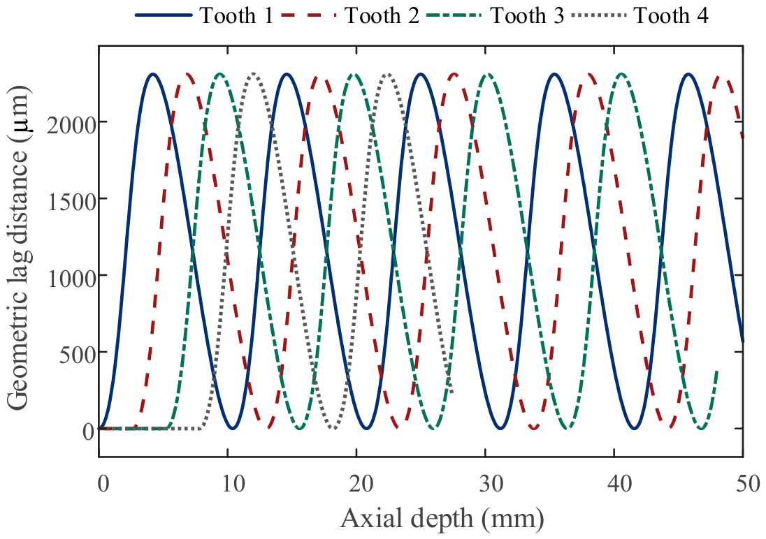
Figure 3 shows the distribution of geometric lag distances of the four cutting edges of the wave-edge milling tool at different axial positions. It can be observed that the geometric lag distance $d_{k,j}$ of each tooth varies periodically with the axial depth, and different teeth exhibit similar variation amplitudes and fluctuation periods. However, due to differences in phase parameters, these curves present an obvious staggered distribution along the axial direction. The local lag angle fluctuation induced by such differences in geometric lag distance directly leads to axial non-uniformity in the pitch angles between adjacent teeth and the corresponding tooth-passing time delays.

To quantitatively describe the local angular position variation induced by waveform undulation, the lag angle of the cutting element of the j-th tooth at the k-th axial discrete layer relative to the reference position of the free-end tool tip of the first tooth is defined as ${\mathrm{\varphi }}_{k,j}$. This lag angle consists of three components: the nominal axial lag angle, the nominal circumferential lag angle, and the additional lag angle caused by the harmonic waveform, which can be expressed as:

$${\varphi }_{\mathrm{k},j}={\varphi }_{k,j}^a+{\varphi }_{k,j}^c+{\varphi }_{k,j}^d$$

(3)

where ${\mathrm{\varphi }}_{k,j}^a$ reflects the axial angular position variation induced by the nominal helix angle, ${\mathrm{\varphi }}_{k,j}^c$ reflects the basic angular position difference caused by the nominal circumferential distribution of the teeth, and ${\mathrm{\varphi }}_{k,j}^d$ is determined by the local lag distance $d_{k,j}$ induced by the waveform profile. According to the aforementioned geometric relationship, they can be further expressed as:

$${\varphi }_{k,j}^a={\displaystyle \frac{(k-1)dz\tan {\theta }_{0j}}{R}}$$

(4)

$${\varphi }_{k,j}^c={\displaystyle \sum _1^{\mathrm{j}}{\phi }_{0j}}$$

(5)

$${\varphi }_{k,j}^d={\displaystyle \frac{d_{k,j}}{R}}$$

(6)

where $d_z$ denotes the height of each axial discrete layer, R denotes the tool radius, and ${\phi }_{0,j}$ denotes the nominal pitch angle.

During the cutting process, when the overall rotation angle of the tool is $\mathrm{\varphi }$, the instantaneous position angle of the cutting element of the j-th tooth at the k-th axial discrete layer can be expressed as:

$${\varphi }_{\mathrm{k},j}(\varphi )={\varphi }_{\mathrm{k},j}+\varphi$$

(7)

Accordingly, the local pitch angle between any two adjacent teeth at the same axial layer can be defined as:

$${\phi }_{k,j-1,j}={\varphi }_{\mathrm{k},j}-{\varphi }_{\mathrm{k},j-1}$$

(8)

The angular wrap-around effect was considered by defining the local pitch angles as cyclic adjacent-tooth intervals. The interval from the fourth tooth to the first tooth includes the nominal pitch distance, which accounts for the closure across the 0/2π boundary.

For conventional milling tools with equal pitch angles, ${\phi }_{k,j-1,j}$ is generally constant. In contrast, for wave-edge milling tools, ${\phi }_{k,j-1,j}$ varies continuously with the axial layer index k. This indicates that the differences in entry time between adjacent teeth are no longer identical at different axial positions, thereby forming a non-uniform inter-tooth engagement characteristic induced by waveform parameters. Therefore, it is necessary to introduce an index capable of quantitatively characterizing the fluctuation level of pitch angles.

2.3. Construction and Physical Meaning of PAV

As discussed in the previous section, the local pitch angle ${\phi }_{k,j-1,j}$ between adjacent teeth of the wave-edge milling tool at the same axial discrete layer is no longer constant, but varies jointly with the axial position and tooth index. It is necessary to introduce a statistical index based on the local pitch angles to reflect the overall fluctuation level. In this study, the pitch angle variance (PAV) proposed by Jiang et al. [20] is adopted as a quantitative characterization index for the time-delay diversity of wave-edge milling tools. Since PAV is defined as the variance of local pitch angles, its unit is rad² when the angular quantities are calculated in radians.

Assuming that there are N pitch angles between adjacent teeth at the k-th axial discrete layer, the average pitch angle of this axial layer can be expressed as:

$$\overline{{\phi }_k}={\displaystyle \frac{1}{N}}{\displaystyle \sum _{j=1}^N{\phi }_{\mathrm{k},j-1,j}}$$

(9)

where ${\phi }_{k,j-1,j}$ denotes the local pitch angle between adjacent teeth $j-1$ and $j$ at the k-th axial discrete layer. On this basis, the variance of pitch angles within the k-th axial layer can be expressed as:

$$V_k={\displaystyle \frac{1}{N}}{\displaystyle \sum _{j=1}^N({\phi }_{\mathrm{k},j-1,j}}-\overline{{\phi }_k}{)}^2$$

(10)

where $V_k$ characterizes the dispersion degree of the pitch angles between adjacent teeth within the k-th axial layer relative to the average value of that layer. A larger $V_k$ indicates more pronounced pitch angle fluctuation within this layer, corresponding to stronger fluctuation in local tooth-passing time delays. Conversely, a smaller $V_k$ indicates that the pitch angle distribution within this layer is closer to uniform.

Considering that the pitch angle distribution of a wave-edge milling tool varies continuously along the axial direction, the variance at a single axial layer is insufficient to reflect the overall time-delay diversity of the tool. Therefore, the variances of all Q axial discrete layers are further averaged, and the pitch angle variance of the cutting elements of the wave-edge milling tool is defined as:

$$V={\displaystyle \frac{1}{Q}}{\displaystyle {\displaystyle \sum _{k=1}^Q}{V}_K}={\displaystyle \frac{1}{Q}}{\displaystyle {\displaystyle \sum _{k=1}^Q}\left[\frac{1}{N}{\displaystyle \sum _{j=1}^N{({\phi }_{\mathrm{k},j-1,j}-\frac{1}{N}{\displaystyle \sum _{j=1}^N{\phi }_{\mathrm{k},j-1,j}})}^2}\right]}$$

(11)

where V is the PAV index, Q denotes the number of axial discrete layers of the tool, and N denotes the number of teeth. This definition is consistent with the previous work of Jiang et al. [20].

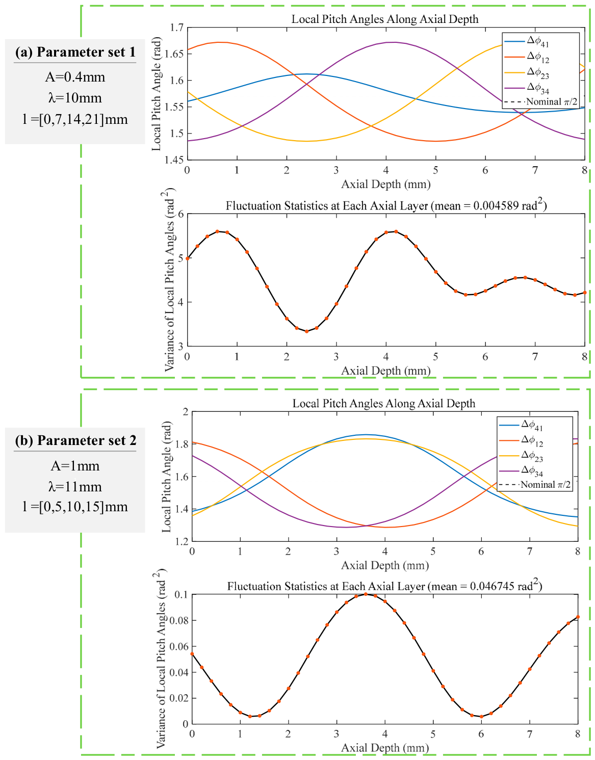
Figure 4 shows the axial distributions of local pitch angles for two representative parameter sets, where the upper figure corresponds to a low-PAV parameter set and the lower figure corresponds to a high-PAV parameter set. It can be observed that, under the low-PAV parameter set, the local pitch angles $\mathsf{\Delta }{\varnothing }_{41}$, $\mathsf{\Delta }{\varnothing }_{12}$, $\mathsf{\Delta }{\varnothing }_{23}$, and $\mathsf{\Delta }{\varnothing }_{34}$ between adjacent teeth only exhibit mild fluctuations with small amplitudes around the nominal pitch angle of 90°, and the overall deviation magnitude at different axial positions remains relatively small. Accordingly, the corresponding variance within each axial layer is also maintained at a low level. In contrast, under the high-PAV parameter set, the deviations of the local pitch angles from the nominal value of 90° become more significant, showing stronger undulation characteristics along the axial direction, and the corresponding variance curves within the axial layers increase as a whole.

3. PAV-Based Stratified Sampling of Waveform Parameters

3.1. Construction of the Feasible Waveform-Parameter Space Under Progressive Phase Distribution

This study adopts progressive phase distribution as the unified phase distribution form. For a four-tooth wave-edge milling tool, the progressive phase distribution can be expressed as $\left(r_1=0,r_2=\mathsf{\Delta }l,r_3=2\mathsf{\Delta }l,r_4=3\mathsf{\Delta }l\right)$, where $\mathsf{\Delta }l$ denotes the phase step between adjacent teeth. However, since the wavelength λ is also treated as an independent variable in this study, directly using the absolute length $\mathsf{\Delta }l$ as the sampling variable would make the phase intensity corresponding to the same value of $\mathsf{\Delta }l$ inconsistent under different wavelength conditions, which is unfavorable for unified comparison among different parameter sets. Therefore, a normalized phase ratio $\mathrm{\xi }=∆l/\lambda$ is further introduced in this study. Accordingly, the progressive phase distribution can be equivalently written as $\left(r_1=0,r_2=\xi \lambda ,r_3=2\xi \lambda {,r}_4=3\xi \lambda \right)$.

The ranges $A\in \left[0,1.5\right]\mathrm{mm}$ and $\lambda \in \left[8,32\right]\mathrm{mm}$ were selected based on the typical geometric window of the wave-edge tools considered in Jiang et al. [20], while avoiding unrealistically large edge undulations or excessively short wave periods that may cause edge interference and manufacturing difficulty. The constraint $\mathsf{\Delta }l\le 8 \mathrm{mm}$ was adopted as a practical upper bound for the adjacent-tooth phase step, where 8 mm corresponds to the minimum wavelength considered in this study. This constraint limits the absolute phase-step magnitude to the scale of the shortest wavelength and keeps the phase design range comparable across different wavelengths. For the phase ratio $\xi$, its value should not only satisfy a reasonable design window of the phase step, but also ensure that the progressive phase distribution does not produce a repeated envelope within a single wavelength period, namely:

$$0\le \xi \le {\xi }_{\max }(\lambda ),{\xi }_{\max }(\lambda )=\min ({\displaystyle \frac{8}{\lambda }},{\displaystyle \frac{1}{3}})$$

(12)

However, the above parameter ranges only provide the initial design window for candidate waveform parameters. The parameter combinations actually used for subsequent PAV calculation and stratified sampling must further satisfy the non-interference condition of the wave-edge geometry. Jiang et al. [20] pointed out that the occurrence of wave-edge interference is jointly determined by the amplitude, wavelength, and nominal helix angle, and the interference avoidance criterion can be written as:

$$\arctan (A_{\mathrm{j}}{a}_j)+{\theta }_{0j}<{\displaystyle \frac{\pi }{2}},a_j={\displaystyle \frac{2\pi }{{\lambda }_j}}$$

(13)

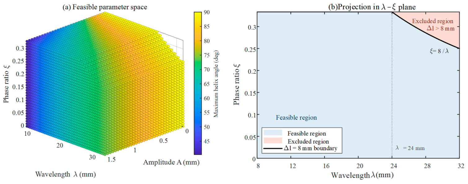
After applying the above constraints, the feasible waveform-parameter space is obtained, as shown in Figure 5. Figure 5a presents the three-dimensional distribution of feasible parameter combinations in the $\left(A,\lambda ,\xi \right)$ space. The color represents the maximum allowable helix angle determined by the wave-edge non-interference condition. Figure 5b further shows the projection of the feasible region in the $\lambda -\xi$ plane. In this projection, the upper boundary is determined by $\Delta l=\xi \lambda \le 8 \mathrm{mm}$ and $\xi \le 1/3$. When $\lambda >24 \mathrm{mm}$, the condition $\Delta l\le 8 \mathrm{mm}$ becomes more restrictive than $\xi \le 1/3$, resulting in the excluded region in the upper-right part of the projection.

It should be emphasized that the proposed PAV-based layered sampling strategy is not inherently restricted to the progressive phase distribution. The progressive distribution is adopted in this study as a controlled and representative phase arrangement, which allows the coupled effects of amplitude, wavelength, and phase ratio to be examined in a unified parameter space. In principle, the same sampling framework can be applied to other phase distribution patterns, such as symmetric or arbitrary phase distributions, as long as the local pitch angles and the corresponding PAV values can be calculated for each parameter set. For a different phase distribution form, the feasible parameter space and the PAV distribution may change, and the layer boundaries should be redefined according to the resulting PAV range and sample density.

3.2. Calculation and Distribution Analysis of PAV

The calculation of PAV relies only on the geometry–delay relationship established in Section 2 and does not require full dynamic stability simulation. It is more suitable as a low-cost geometric descriptor for probability-biased pre-screening in the parameter space. Based on the defined feasible waveform-parameter space, high-throughput computation is adopted in this study to evaluate PAV for a large number of candidate parameter sets.

To reveal the overall distribution characteristics of PAV in the feasible parameter space, the PAV results of all samples were statistically analyzed. The analysis mainly includes the overall value range, frequency distribution, and dispersion degree of PAV, as well as the relative distribution characteristics of high- and low-PAV samples in the parameter space.

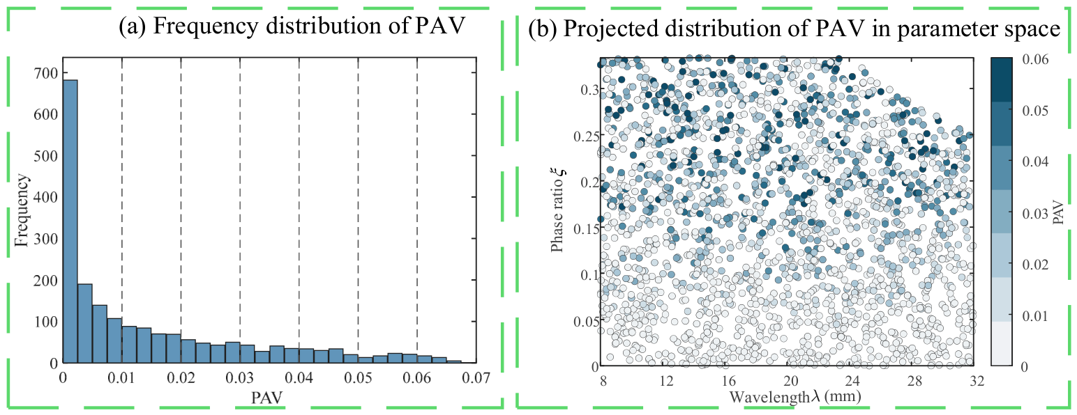
As shown in Figure 6, PAV exhibits a significantly non-uniform distribution within the feasible parameter space. The frequency statistics indicate that most samples are concentrated in the low-PAV region, and the overall distribution shows an evident right-skewed characteristic. This phenomenon can be attributed to the restrictive effect of the geometric feasibility constraints on high-PAV parameter combinations. A large PAV generally requires a relatively large amplitude, a short wavelength, and a sufficiently large phase shift among adjacent teeth. However, these conditions also increase the local edge slope, lag-angle fluctuation, and possibility of wave-edge interference. Therefore, only a limited portion of the feasible parameter space can generate strong pitch-angle dispersion, whereas most manufacturable parameter combinations produce relatively mild pitch-angle fluctuation and fall into the low-PAV region. This interpretation is consistent with studies on serrated and harmonically varied milling tools, where the attainable time-delay distribution is strongly constrained by edge-profile continuity, local helix-angle variation, phase arrangement, and chip-thickness redistribution [21,22,23,24]. Therefore, the concentration of samples in the low-PAV region is not only a statistical phenomenon, but also a consequence of the geometric feasibility constraints imposed on wave-edge tool design.

The projection results in the parameter space further show that the response of PAV to wavelength and normalized phase ratio exhibits a certain degree of dispersion. Nevertheless, high-PAV samples generally appear more frequently in regions with larger phase ratios, indicating that the phase progression ratio has a more direct influence on the formation of time-delay diversity. Figure 6 indicates that low-PAV parameter combinations occupy the dominant proportion in the feasible parameter space, whereas high-PAV combinations are relatively sparse.

3.3. PAV-Based Stratified Sampling Strategy

Based on the global distribution characteristics of PAV shown in Figure 6, stratified sampling was conducted in this study according to different PAV value levels. Within each layer, instead of selecting only three representative parameter sets corresponding to the lower end, middle region, and upper end of the interval, each of these three subregions was further sampled to retain three representative parameter sets. In this way, nine representative samples were obtained from each layer, corresponding to the lower-end, mid-range, and upper-end portions of the interval, respectively.

Combined with the frequency distribution of PAV shown in Figure 6a, the main sample-concentrated interval $V\in \left[\mathrm{0,0.06}\right]$ was selected as the formal stratification range in this study and was evenly divided into six layers. Layers 1 to 6 correspond to the PAV intervals of 0–0.01, 0.01–0.02, 0.02–0.03, 0.03–0.04, 0.04–0.05, and 0.05–0.06, respectively. For a small number of high-value tail samples falling within $V>0.06$, they were not included in the formal stratified statistics because of their extremely limited quantity and their unsuitability for balanced inter-layer comparison. Instead, these samples were retained as supplementary extreme cases and are discussed in Section 5.3 as high-value tail conditions to examine the boundary behavior of PAV.

If multiple samples within a given layer exhibit similar deviations from the target value, samples with larger differences in parameter combinations are preferentially retained to avoid excessive clustering of representative parameters in the $\left(A,\lambda ,\xi \right)$ space. Finally, through the above stratified sampling method, a total of 54 representative waveform-parameter samples were selected from the six PAV layers for the stability solution and SRA calculation in Section 4. The 54 samples were not intended to construct a high-accuracy predictive surrogate model. Instead, they were selected to retain representative low-, medium-, and high-PAV cases for comparative SLD/SRA evaluation at a manageable computational cost.

To quantitatively examine the coverage of the selected samples, the parameter-span coverage ratio was calculated by comparing the range of the 54 representative samples with that of the 2000 feasible candidate combinations. The selected samples cover 87.0% of the amplitude range, 98.2% of the wavelength range, 90.4% of the phase-ratio range, and 90.9% of the adjacent-tooth phase-step range of the full candidate set. For PAV, the selected samples cover 96.9% of the formal PAV range below 0.06. Therefore, the 54 samples retain broad coverage of both the waveform-parameter space and the PAV-layer space.

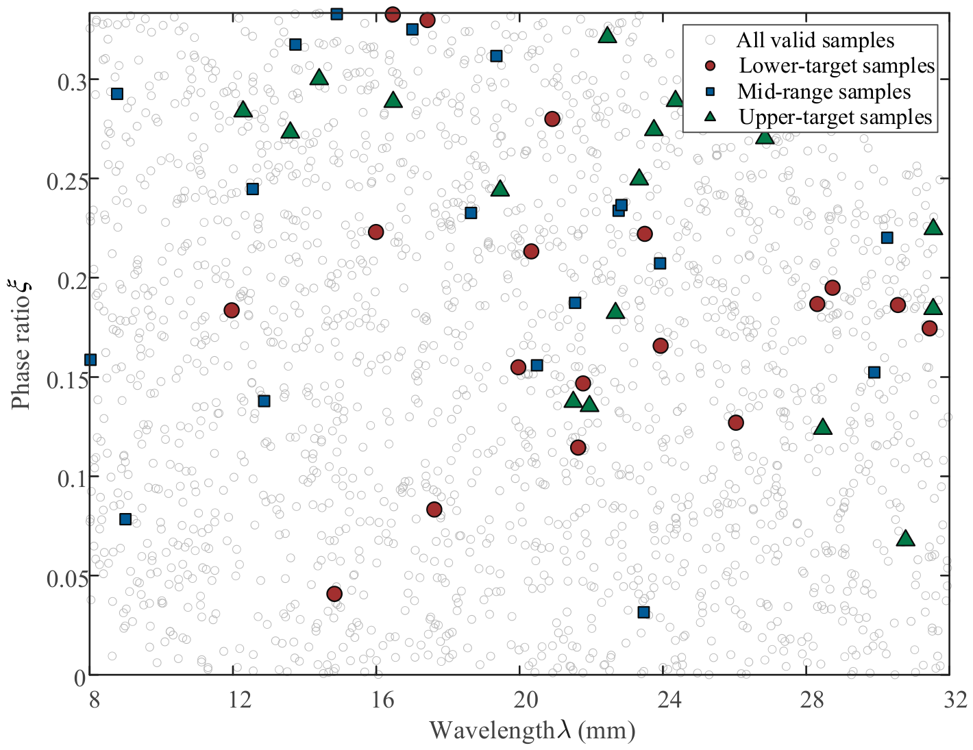
As shown in Figure 7, to verify whether the PAV-based stratified sampling strategy can maintain representativeness in the parameter space while ensuring computational efficiency, the 54 representative parameter samples were further projected onto the wavelength–phase-ratio parameter plane for visualization. In the figure, the light-gray hollow circles represent all feasible parameter sets, while the colored solid circles, squares, and triangles represent the lower-target samples, mid-range samples, and upper-target samples selected from each PAV layer, respectively. It can be observed that the 54 selected representative samples do not exhibit obvious local clustering, but instead maintain good distribution coverage over the entire feasible parameter space. Meanwhile, the three types of samples within different layers also show certain differences in the parameter space, indicating that the proposed sampling strategy not only preserves the inter-layer information among different PAV levels, but also retains, to some extent, the intra-layer gradient variation characteristics.

For subsequent stability evaluation and inter-layer statistical analysis,

Table 1. Lower-end target samples.

Layer	PAV Interval	ID	A (mm)	$\mathit{\lambda }$ (mm)	$\mathit{\xi }$	PAV
1	[0, 0.01]	L1-1	0.1792	30.5615	0.1863	8.3546 × 10−4
1	[0, 0.01]	L1-2	0.7983	14.8339	0.0408	1.67872 × 10−3
1	[0, 0.01]	L1-3	0.3432	23.9385	0.1658	2.50533 × 10−3
2	[0.01, 0.02]	L2-1	0.8282	21.6354	0.1145	1.077578 × 10−2
2	[0.01, 0.02]	L2-2	0.7690	21.7733	0.1468	1.167047 × 10−2
2	[0.01, 0.02]	L2-3	0.6934	11.9648	0.1836	1.248099 × 10−2
3	[0.02, 0.03]	L3-1	0.8657	20.9131	0.2800	2.088428 × 10−2
3	[0.02, 0.03]	L3-2	1.3639	17.6210	0.0833	2.167192 × 10−2
3	[0.02, 0.03]	L3-3	1.0020	19.9659	0.1549	2.253780 × 10−2
4	[0.03, 0.04]	L4-1	1.4615	26.0401	0.1270	3.082285 × 10−2
4	[0.03, 0.04]	L4-2	1.1135	28.7373	0.1950	3.159384 × 10−2
4	[0.03, 0.04]	L4-3	1.0606	15.9922	0.2230	3.248021 × 10−2
5	[0.04, 0.05]	L5-1	1.2108	23.4953	0.2221	4.080959 × 10−2
5	[0.04, 0.05]	L5-2	1.3922	31.4460	0.1745	4.163770 × 10−2
5	[0.04, 0.05]	L5-3	1.1624	17.4310	0.3298	4.246647 × 10−2
6	[0.05, 0.06]	L6-1	1.3567	20.3272	0.2133	5.087188 × 10−2
6	[0.05, 0.06]	L6-2	1.4796	28.3098	0.1868	5.154619 × 10−2
6	[0.05, 0.06]	L6-3	1.2943	16.4608	0.3326	5.237192 × 10−2

,

Table 2. Mid-range target samples.

Layer	PAV Interval	ID	A (mm)	$\mathit{\lambda }$ (mm)	$\mathit{\xi }$	PAV
1	[0, 0.01]	M1-1	1.3410	23.4659	0.0315	4.16912 × 10−3
1	[0, 0.01]	M1-2	0.4464	21.5506	0.1874	4.98843 × 10−3
1	[0, 0.01]	M1-3	0.8101	8.9993	0.0784	5.83198 × 10−3
2	[0.01, 0.02]	M2-1	0.6776	17.0104	0.3251	1.414659 × 10−2
2	[0.01, 0.02]	M2-2	0.9410	29.9009	0.1523	1.499136 × 10−2
2	[0.01, 0.02]	M2-3	0.7297	13.7459	0.3175	1.582854 × 10−2
3	[0.02, 0.03]	M3-1	0.9300	22.7653	0.2337	2.428983 × 10−2
3	[0.02, 0.03]	M3-2	0.9169	19.3553	0.3117	2.502196 × 10−2
3	[0.02, 0.03]	M3-3	0.9111	14.8993	0.3328	2.581296 × 10−2
4	[0.03, 0.04]	M4-1	1.1024	18.6441	0.2326	3.439987 × 10−2
4	[0.03, 0.04]	M4-2	1.3244	12.8705	0.1379	3.503210 × 10−2
4	[0.03, 0.04]	M4-3	1.2663	20.4856	0.1559	3.582607 × 10−2
5	[0.04, 0.05]	M5-1	1.2378	8.7676	0.2927	4.415444 × 10−2
5	[0.04, 0.05]	M5-2	1.4115	8.0248	0.1587	4.500057 × 10−2
5	[0.04, 0.05]	M5-3	1.2691	30.2619	0.2202	4.588687 × 10−2
6	[0.05, 0.06]	M6-1	1.3835	22.8440	0.2366	5.436579 × 10−2
6	[0.05, 0.06]	M6-2	1.3780	12.5504	0.2447	5.495548 × 10−2
6	[0.05, 0.06]	M6-3	1.4473	23.9226	0.2072	5.581055 × 10−2

and

Table 3. High-end target samples.

Layer	PAV Interval	ID	A (mm)	$\mathit{\lambda }$ (mm)	$\mathit{\xi }$	PAV
1	[0, 0.01]	H1-1	1.1857	30.7763	0.0677	7.51283 × 10−3
1	[0, 0.01]	H1-2	0.5451	16.4730	0.2885	8.31789 × 10−3
1	[0, 0.01]	H1-3	0.6184	22.6771	0.1823	9.18115 × 10−3
2	[0.01, 0.02]	H2-1	0.7875	14.4068	0.3000	1.752301 × 10−2
2	[0.01, 0.02]	H2-2	0.9822	21.4992	0.1375	1.836440 × 10−2
2	[0.01, 0.02]	H2-3	1.2543	28.4657	0.1239	1.916207 × 10−2
3	[0.02, 0.03]	H3-1	1.0024	24.3526	0.2890	2.751444 × 10−2
3	[0.02, 0.03]	H3-2	1.2295	21.9517	0.1354	2.832183 × 10−2
3	[0.02, 0.03]	H3-3	1.0973	31.5435	0.1843	2.913458 × 10−2
4	[0.03, 0.04]	H4-1	1.1886	27.0859	0.2907	3.765965 × 10−2
4	[0.03, 0.04]	H4-2	1.1925	26.8480	0.2703	3.842475 × 10−2
4	[0.03, 0.04]	H4-3	1.1649	31.5490	0.2245	3.928033 × 10−2
5	[0.04, 0.05]	H5-1	1.3096	23.7488	0.2743	4.740066 × 10−2
5	[0.04, 0.05]	H5-2	1.3106	19.4585	0.2439	4.864014 × 10−2
5	[0.04, 0.05]	H5-3	1.2673	22.4524	0.3212	4.914101 × 10−2
6	[0.05, 0.06]	H6-1	1.4239	23.3404	0.2495	5.754003 × 10−2
6	[0.05, 0.06]	H6-2	1.4346	13.6003	0.2731	5.824588 × 10−2
6	[0.05, 0.06]	H6-3	1.4557	12.2833	0.2838	5.894120 × 10−2

summarize the 54 representative waveform-parameter samples selected by the PAV-based stratified sampling strategy. Table 1, Table 2 and Table 3 correspond to the lower-end target samples, mid-range target samples, and high-end target samples of each PAV layer, respectively. For each PAV layer, three lower-end target samples, three mid-range target samples, and three high-end target samples were selected, resulting in nine representative samples per layer and 54 samples in total. These samples cover the formal PAV range of $V\in \left[\mathrm{0,0.06}\right]$ and were used for subsequent high-fidelity stability lobe diagram construction and SRA extraction.

4. Stability Prediction Framework and Quantitative Evaluation Index

4.1. Multi-Delay Dynamic Model of Wave-Edge Milling

To ensure consistency in stability evaluation among different representative parameter samples, this study adopts the wave-edge milling dynamic model established and experimentally validated by Jiang et al. [20] based on the explicit geometric modeling framework as the basis for stability prediction. This model takes the local pitch angles and local tooth-passing time delays obtained in Section 2 as geometric inputs, and characterizes the regenerative dynamic behavior of the wave-edge milling system within a multi-modal framework. Since the corresponding modeling procedure has been systematically derived in the aforementioned literature, the complete derivation is not repeated in this study. Instead, only the dynamic equations and key variable definitions directly related to the subsequent stability solution are retained. To facilitate the subsequent stability analysis, the system is formulated in modal coordinates using modal superposition, in which the structural dynamic characteristics and the regenerative cutting-force terms are uniformly incorporated into a time-delay state equation.

Let the generalized displacement vector of the tool–spindle system in the cutting plane be $q\left(t\right)$. The dynamic equation of the wave-edge milling system can then be written as:

$$\mathit{M}\ddot{\mathit{q}}(t)+\mathit{C}\dot{\mathit{q}}(t)+\mathit{K}\mathit{q}(t)=\mathit{F}(t)$$

(14)

where M, C, and K denote the mass, damping, and stiffness matrices of the system, respectively, and $\mathit{F}\left(t\right)$ denotes the time-varying cutting-force vector jointly generated by the cutting elements of all teeth. Considering that the cutting edges of the wave-edge milling tool exhibit continuous harmonic undulations along the axial direction, and that the local helix angle, local pitch angle, and local tooth-passing time delay at different axial heights vary with the waveform parameters, the cutting force $\mathit{F}\left(t\right)$ should be obtained by summing the contributions of all axial discrete layers and tooth cutting elements.

Under regenerative milling conditions, the chip thickness depends not only on the instantaneous displacement of the cutting element of the current tooth, but also on the historical displacement of the preceding adjacent tooth after the corresponding local time delay. The dynamic undeformed chip thickness at the cutting element of the j-th tooth and the k-th axial discrete layer can be expressed as the projection of the difference between the current displacement and the delayed displacement, namely:

$$h_{k,j}(t)=h_{0,k,j}(t)+{\mathit{n}}_{k,j}^T\left[\mathit{q}(t)-\mathit{q}(t-{\tau }_{k,j-1,j})\right]$$

(15)

where $h_{0,k,j}\left(t\right)$ denotes the static undeformed chip thickness determined by tool kinematics and feed motion, ${\mathit{n}}_{k,j}$ denotes the normal direction vector of the corresponding cutting element, and ${\tau }_{k,j-1,j}$ is the local tooth-passing time delay defined in Section 2. The above equation indicates that the regenerative term in wave-edge milling no longer corresponds to a single fixed time delay, but is jointly determined by the local time delays associated with different axial layers and different tooth pairs.

After summing the cutting-force contributions corresponding to all axial discrete layers and tooth cutting elements, the equation can be further written in a matrix form containing multiple time-delay terms:

$$\mathit{M}\ddot{\mathit{q}}(t)+\mathit{C}\dot{\mathit{q}}(t)+\mathit{K}\mathit{q}(t)={\displaystyle {\displaystyle \sum _{j=1}^{N_t}}{\displaystyle \sum _{k-1}^Q{\mathit{G}}_{k,j}}}(t)\mathit{q}(t)-{\displaystyle {\displaystyle \sum _{j=1}^{N_t}}{\displaystyle \sum _{k-1}^Q{\mathit{H}}_{k,j}}}(t)\mathit{q}(t-{\tau }_{k,j-1,j})$$

(16)

where $N_t$ denotes the number of teeth and Q denotes the number of axial discrete layers. ${\mathit{G}}_{k,j}\left(t\right)$ and ${\mathit{H}}_{k,j}\left(t\right)$ represent the time-varying coefficient matrices associated with the current displacement term and the delayed displacement term, respectively, whose specific forms are jointly determined by the cutting-force model, local cutting geometry, and tooth engagement state. Since ${\tau }_{k,j-1,j}$ varies with the axial layer k and tooth index j, the above equation essentially constitutes a multi-delay and multi-modal periodic time-varying dynamic system.

4.2. Stability Solution and Stability Lobe Diagram Construction Based on the Semi-Discretization Method

Based on the established multi-delay dynamic model, the semi-discretization method was adopted in this study as a unified stability evaluation tool for the representative parameter samples. The numerical stability of the wave-edge milling system was then solved, and the corresponding stability lobe diagrams were constructed accordingly.

The present study focuses on numerical parameter screening based on the previously validated dynamic model reported by Jiang et al. [20], rather than on new cutting experiments. To improve the reproducibility of the SLD/SRA calculations, the main simulation parameters used in the stability evaluation are summarized in

Table 4. Simulation parameters used for SLD/SRA evaluation.

Category	Parameter	Value
Tool geometry	Tool diameter, D	16 mm
Tool geometry	Number of teeth, $N_t$	4
Tool geometry	Nominal helix angle, ${\theta }_0$	30°
Cutting condition	Workpiece material	TC4 titanium alloy
Cutting condition	Milling mode	Down milling
Cutting condition	Radial depth of cut, $a_e$	4 mm
Stability map settings	Spindle speed range, n	2000–8000 rpm
Stability map settings	Axial depth of cut range, $a_p$	0–8 mm
Stability map settings	Axial-depth increment, $∆a_p$	0.1 mm
Stability map settings	Spindle-speed grid points, $N_n$	101
Stability map settings	Spindle-speed increment, $∆n$	60 rpm
Stability map settings	axial-depth grid points, $N_{a_p}$	81
Cutting force coefficients	Tangential coefficient, $K_t$	1533.35 N/mm2
Cutting force coefficients	Radial coefficient, $K_n$	631.90 N/mm2
Structural dynamics	Natural frequency in x direction, $f_{nx}$	1177.35 Hz, 2228.56 Hz
Structural dynamics	Natural frequency in y direction, $f_{ny}$	914.551 Hz, 1052.21 Hz, 2203.53 Hz
Structural dynamics	Damping ratio in x direction, ${\zeta }_x$	0.0372, 0.0337
Structural dynamics	Damping ratio in y direction, ${\zeta }_y$	0.0342, 0.0416, 0.0454
Structural dynamics	Modal stiffness in x direction, $k_x$	1.6446 × 107 N/m, 2.2330 × 107 N/m
Structural dynamics	Modal stiffness in y direction, $k_y$	5.6145 × 107 N/m, 3.8574 × 107 N/m, 1.7737 × 107 N/m

, including the tool geometry, cutting conditions, stability-map settings, cutting force coefficients, and structural dynamic parameters. These parameters were kept identical for all representative waveform-parameter samples.

The cutting force coefficients listed in Table 4 were adopted from the experimentally validated dataset of Jiang et al. [20], in which the coefficients were calibrated through standard-tool slot-milling tests using the same workpiece material and comparable tool parameters as the wave-edge tools, with milling forces measured by a KISTLER 9257B dynamometer. The detailed calibration and verification conditions, including spindle speed, feed engagement, axial depth of cut, radial depth of cut, and milling mode, are reported in the experimental section of Jiang et al. [20]. In the present two-dimensional stability calculation, the tangential and radial coefficients are incorporated into the wave-edge force model through the local cutting geometry, local helix-angle variation, tooth engagement state, and axial-layer summation. Therefore, no new force-coefficient calibration was performed in the present numerical study.

In this study, SRA is calculated on the spindle speed–axial depth plane of the stability lobe diagram. The spindle speed range is 2000–8000 rpm, and the axial depth of cut range is 0–8 mm. The spindle speed direction is discretized into 101 grid points with a step of 60 rpm, while the axial depth direction is discretized into 81 grid points with a step of 0.1 mm. For each grid point, the stability state is determined using the semi-discretization method and the Floquet stability criterion. A grid point is regarded as stable when the maximum modulus of the eigenvalues of the single-period transition matrix is smaller than 1. The SRA is then calculated by summing the area of all stable grid cells. Mathematically, the grid-based SRA can be expressed as:

$$\mathrm{SRA}={\displaystyle \sum _{i=1}^{N_n}{\displaystyle \sum _{j=1}^{N_{a_p}}I(n_i,a_{p,j})}}\Delta n\Delta a_p=N_S\Delta n\Delta a_p$$

(17)

where $N_n$ and $N_{a_p}$ are the numbers of grid points in the spindle-speed and axial-depth directions, respectively. In this study, $N_n=101$ and $N_{a_p}=81$. $n_i$ denotes the $i$-th spindle speed, and $a_{p,j}$ denotes the $j$-th axial depth of cut. $I\left(n_i,a_{p,j}\right)$ is the stability indicator function, where $I=1$ if the grid point is stable and $I=0$ otherwise. $N_s$ is the total number of stable grid points, $\mathsf{\Delta }n=60$ rpm is the spindle-speed step, and $\mathsf{\Delta }{a}_p=1\times {10}^{-4}$ m is the axial-depth step. The calculated SRA values are reported in units of $\mathrm{r}\mathrm{p}\mathrm{m}\cdot \mathrm{m}$, and the SRA is not normalized.

To facilitate the application of the semi-discretization method, the multi-delay dynamic equation shown in Equation (16) is rewritten into a first-order state-space form. The system state vector is defined as:

$$\mathbf{x}(t)=\left[\begin{array}{l}\mathit{q}(t)\\ \dot{\mathit{q}}(t)\end{array}\right]$$

(18)

Then, the wave-edge milling system can be uniformly expressed as:

$$\dot{\mathit{x}}(t)=\mathit{A}(t)\mathit{x}(t)+{\displaystyle \sum _{p=1}^{N_d}{\mathit{B}}_p}(t)\mathit{x}(t-{\tau }_p)$$

(19)

where $\mathit{A}\left(t\right)$ denotes the time-varying coefficient matrix associated with the current state, ${\mathit{B}}_p\left(t\right)$ denotes the coefficient matrix corresponding to the p-th local time-delay term, $N_d$ represents the total number of local time-delay terms involved in the regenerative effect, and ${\tau }_p$ is the set of local tooth-passing time delays defined in Section 2. Since the local pitch angles and local tooth-passing time delays are not constant among different axial layers and different tooth pairs, Equation (18) essentially corresponds to a periodic time-varying delay differential equation with multiple time-delay terms.

Let the spindle angular velocity be $\Omega$. Then, one tooth-passing period can be expressed as:

$$T_o={\displaystyle \frac{2\pi }{N_t\Omega }}$$

(20)

where $N_t$ denotes the number of teeth. According to the semi-discretization method, one tooth-passing period $T_0$ is uniformly divided into m discrete subintervals, and the length of each subinterval is given by:

$$\mathrm{\Delta }t={\displaystyle \frac{T_0}{m}}$$

(21)

In the present calculation, each tooth-passing period was divided into m = 160 subintervals. Since the spindle speed range was 2000–8000 rpm, the corresponding time step Δt varied from 1.875 × 10⁻⁴ s to 4.6875 × 10⁻⁵ s according to the spindle speed.

Within each discrete interval $[t_i,t_{i+1})$, the time-varying coefficient matrices $A\left(t\right)$ and $B_p\left(t\right)$ are assumed to be approximated as piecewise constants, namely, the continuously varying coefficient matrices are replaced by the representative values ${\mathit{A}}_i$ and ${\mathit{B}}_{p,i}$ within the interval. In this way, the original periodic time-varying delay system can be approximated as a constant-coefficient multi-delay system in each time subinterval, thereby facilitating the construction of the discrete state mapping.

For any local time delay ${\tau }_p$, it can be written as:

$${\tau }_p=(l_p+{\alpha }_p)\mathrm{\Delta }t,0\le {\alpha }_p<1$$

(22)

where $l_p$ is the integer number of discrete steps corresponding to the time delay, and ${\alpha }_p$ is the remaining fractional part. Since ${\tau }_p$ generally does not exactly coincide with a discrete node, the semi-discretization method uses linear interpolation between two adjacent historical nodes to approximate the delayed state, namely:

$$\mathit{x}(t_i-{\tau }_p)\approx (1-{\alpha }_p){\mathit{x}}_{i-l_p}+{\alpha }_p{\mathit{x}}_{i-l_p-1}$$

(23)

where ${\mathit{x}}_{i-l_p}$ and ${\mathit{x}}_{i-l_p-1}$ denote the two discrete historical states adjacent to the delayed instant, respectively. Through the above interpolation, the continuous time-delay term is transformed into a linear combination of several discrete historical states, so that a discrete recursive relationship can be established within each discrete interval.

Substituting Equation (22) into Equation (18) and applying the semi-discretization approximation within each discrete interval, the following discrete state recursive form can be obtained:

$${\mathit{x}}_{i+1}={\mathit{P}}_i{\mathit{x}}_i+{\displaystyle \sum _{p=1}^{N_d}({\mathit{H}}_{p,i}^{(0)}{\mathit{x}}_{i-l_p}+{\mathit{H}}_{p,i}^{(1)}{\mathit{x}}_{i-l_p-1})}$$

(24)

where ${\mathit{P}}_i$ denotes the discrete transition matrix of the current state term, and ${\mathit{H}}_{p,i}^{\left(0\right)}$ and ${\mathit{H}}_{p,i}^{\left(1\right)}$ represent the discrete weighting matrices of the p-th time-delay term at two adjacent historical nodes, respectively. To further construct a standard discrete mapping, the current state and the required historical states are combined into an augmented state vector, namely:

$${\mathit{X}}_i={\left[{\mathit{x}}_i^T,{\mathit{x}}_i^T,\dots ,{\mathit{x}}_{i-L}^T\right]}^T$$

(25)

where L is the maximum number of historical steps required to be retained. Accordingly, the equation can be further written as:

$${\mathit{X}}_{i+1}={\mathit{\Psi }}_i{\mathit{X}}_i$$

(26)

where ${\mathit{\Psi }}_i$ denotes the augmented state transition matrix corresponding to the i-th discrete interval. By successively multiplying the transition matrices of all m discrete intervals within one tooth-passing period, the single-period state transition matrix can be obtained as:

$$\mathit{\Phi }={\mathit{\Psi }}_{m-1}{\mathit{\Psi }}_{m-2}\dots {\mathit{\Psi }}_1{\mathit{\Psi }}_0$$

(27)

This matrix is the single-period mapping matrix used for stability judgment based on Floquet theory.

Based on Floquet theory, the system stability can be determined by the spectral radius of the matrix Φ. Let ${\mu }_{max}$ denote the maximum modulus of the eigenvalues of Φ; then, the following criterion can be obtained:

$$\rho (\mathit{\Phi })=\left|{\mu }_{\max }\right|$$

(28)

When $\rho \left(\mathit{\Phi }\right)<1$, the system is stable; when $\rho \left(\mathit{\Phi }\right)>1$, the system becomes unstable; and $\rho \left(\mathit{\Phi }\right)=1$ corresponds to the stability boundary.

5. Results and Discussion

Based on the 54 representative waveform-parameter samples obtained in Section 3 and the unified stability evaluation framework established in Section 4, this section further systematically analyzes the relationship between PAV and milling stability from four aspects: the global correspondence, inter-layer statistical characteristics, comparison of stability lobe diagrams under typical working conditions, and the discussion of mechanisms and applicability boundaries.

5.1. Correlation Between PAV and SRA Under the Sampling Framework

Before analyzing the relationship between PAV and SRA, the computational efficiency of the proposed framework must be evaluated. In the present parameter space, 2000 feasible waveform-parameter combinations were randomly generated. If high-fidelity SLD/SRA evaluation is directly performed for all feasible combinations, 2000 stability lobe diagrams need to be constructed. Since the average computational time for one SLD/SRA calculation is about 242 s, the full direct evaluation would require approximately 134.4 h. In contrast, the proposed PAV-based layered sampling strategy only requires high-fidelity SLD/SRA evaluation for 54 representative samples, corresponding to approximately 3.6 h of computation. The number of high-fidelity stability evaluations is reduced from 2000 to 54, giving a reduction of about 97.3% in the dominant SLD/SRA computational cost.

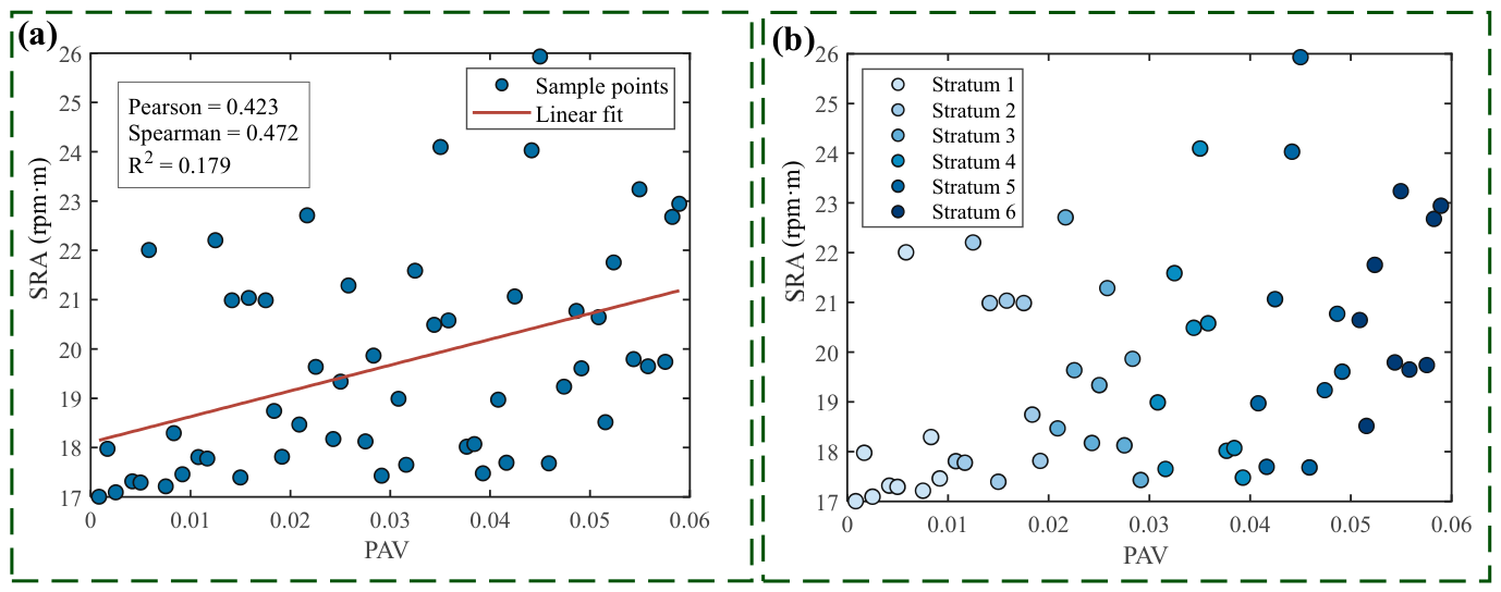
As shown in Figure 8a, the 54 representative samples exhibit an overall positive but scattered distribution trend in the PAV–SRA plane. The linear fitting results indicate that the pointwise correlation between PAV and SRA is weak under the coupled waveform-parameter space. The corresponding Pearson correlation coefficient is 0.4234, the Spearman rank correlation coefficient is 0.4720, and the coefficient of determination is R² = 0.179. This low R² value indicates that PAV alone cannot quantitatively predict the SRA of an individual waveform-parameter set. Therefore, PAV should not be interpreted as a deterministic prediction model or a stand-alone stability selection criterion. Furthermore, Figure 8b presents the sample distribution after PAV stratification. It can be observed that samples from different layers do not form strictly separated banded regions in the PAV–SRA plane, but instead exhibit a certain degree of overlap. A larger PAV does not guarantee a larger SRA for every individual sample. However, the distribution still suggests a statistical tendency that higher-PAV layers are more likely to contain larger-SRA samples, which motivates the subsequent stratified probability analysis.

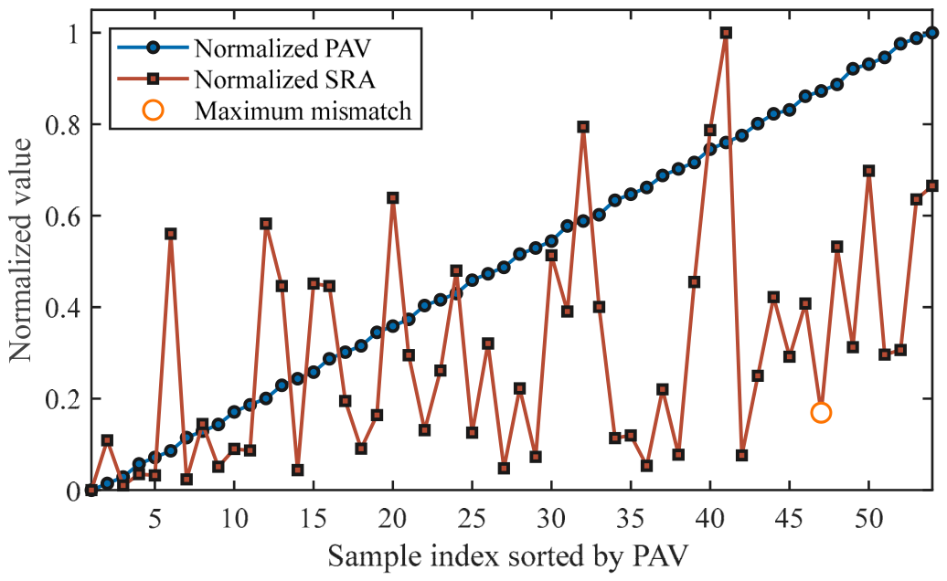
Figure 9 further compares the variation trends of normalized PAV and normalized SRA after the 54 samples are sorted in ascending order of PAV. Since the horizontal axis is ordered according to PAV, the normalized PAV increases monotonically with the sample index. In contrast, the normalized SRA does not exhibit a synchronous monotonic increasing trend, but only shows locally consistent variations amid overall fluctuations. Particularly in the medium- and high-PAV regions, the SRA values corresponding to different samples may still vary considerably. Even when samples have similar pitch-angle fluctuation levels, their final stability performance may differ due to the coupled effects of amplitude, wavelength, phase, and dynamic response characteristics.

5.2. Layer-by-Layer Statistical Analysis

Although the pointwise PAV–SRA relationship is weak at the individual-sample level, the scatter distribution still shows an overall positive tendency. Therefore, it is necessary to further return to the stratified sampling framework constructed in Section 3 and examine the distribution characteristics of stability responses at different PAV levels from the perspective of inter-layer statistics.

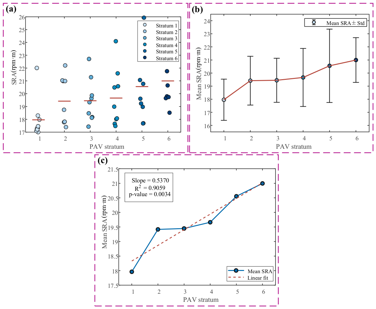
As shown in Figure 10a, the SRA distributions corresponding to different PAV layers exhibit certain inter-layer differences. Overall, the samples in Layer 1 are mainly concentrated in the lower-SRA region, whereas higher SRA values appear more frequently in the medium- and high-PAV layers. However, the samples from different layers do not form clearly separated banded structures. Some samples from the medium and high layers still fall within the lower-SRA region, and evident overlap also exists between adjacent layers.

Figure 10b further presents the mean values and standard deviations of SRA for different layers. Compared with Layer 1, the average SRA values of Layers 2 to 6 are generally increased, while some layers still exhibit relatively large standard deviations.

To examine the evolution of layer-averaged SRA with increasing PAV levels, Figure 10c plots the trend curve of the average SRA for each layer as a function of the layer index. The results show that the mean SRA increases monotonically from 17.962 in Layer 1 to 20.996 in Layer 6, in units of $\mathrm{r}\mathrm{p}\mathrm{m}\cdot \mathrm{m}$. The linear trend analysis gives a positive slope of 0.5370, with $R^2=0.9059$ and $p=0.0034$. This result further suggests that samples in higher-PAV layers have a higher statistical tendency to achieve larger stability regions, although the intra-layer dispersion indicates that this tendency is not deterministic at the individual-sample level.

The mean, standard deviation, median, and value range of SRA for each layer are summarized in

Table 5. Statistical summary of SRA for each PAV layer.

Layer	PAV Interval	Sample Number	Mean SRA (rpm·m)	Std. Dev. (rpm·m)	Median (rpm·m)
1	[0, 0.01]	9	17.962	1.574	17.316
2	[0.01, 0.02]	9	19.417	1.862	18.744
3	[0.02, 0.03]	9	19.449	1.683	19.338
4	[0.03, 0.04]	9	19.663	2.219	18.990
5	[0.04, 0.05]	9	20.555	2.804	19.608
6	[0.05, 0.06]	9	20.996	1.708	20.646

. As shown in Table 5, Layer 1 exhibits the lowest average SRA, whereas Layers 3, 5, and 6 generally show higher average SRA values, which is consistent with the overall upward trend across layers observed in Figure 10. To further evaluate the probability-biased screening capability of PAV, the probabilities of obtaining above-median, above-mean, and top-quartile SRA values are summarized in

Table 6. Probability of obtaining large-SRA samples in different PAV layers.

Layer	Mean SRA (rpm·m)	Median SRA (rpm·m)	P (SRA > Global Median)	P (SRA > Global Mean)	P (SRA in Top 25%)
1	17.962	17.316	11.1%	11.1%	11.1%
2	19.417	18.744	44.4%	44.4%	22.2%
3	19.449	19.338	55.6%	33.3%	22.2%
4	19.663	18.990	44.4%	44.4%	22.2%
5	20.555	19.608	55.6%	44.4%	33.3%
6	20.996	20.646	88.9%	77.8%	44.4%

.

As shown in Table 6, the global median SRA of the 54 samples is 19.287 rpm·m, and the global mean SRA is 19.674 rpm·m. The probability of obtaining an above-median SRA increases from 11.1% in Layer 1 to 88.9% in Layer 6, while the probability of obtaining an above-mean SRA increases from 11.1% to 77.8%. In addition, the probability of obtaining a top-quartile SRA increases from 11.1% in Layer 1 to 44.4% in Layer 6. These results suggest that, although PAV cannot predict individual SRA values, the present sample set exhibits a layer-wise statistical tendency that may provide auxiliary information for preliminary candidate prioritization.

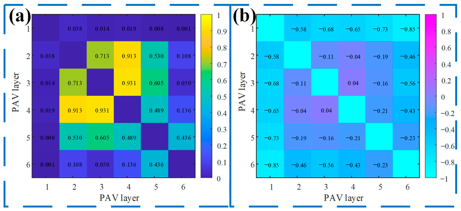
Figure 11 presents the results of the nonparametric pairwise comparisons among different PAV layers. The Mann–Whitney U test is used to evaluate whether the SRA distributions between two layers show a significant difference, while Cliff’s delta is adopted to quantify the corresponding effect size and distributional difference. As shown in Figure 11a, the pairwise p-values indicate that the differences between adjacent layers are not always statistically significant, which is consistent with the overlap of SRA distributions observed in Figure 10a. However, comparisons involving layers with larger PAV separation generally show clearer distributional differences. Figure 11b further confirms this tendency from the perspective of effect size. These results suggest that PAV stratification can capture a layer-wise probabilistic tendency of SRA variation, although the stability performance of individual samples is still governed by the coupled waveform parameters and the dynamic response of the milling system.

Combining Figure 10, Figure 11, Table 5 and Table 6, it can be concluded that PAV stratification should not be regarded as a strict stability classification criterion. Its main value lies in probability-biased pre-screening: higher-PAV layers have a higher probability of containing large-SRA samples, but overlap still exists between adjacent layers and the intra-layer dispersion remains noticeable. Therefore, PAV stratification is more suitable for prioritizing candidate regions and reducing the number of high-fidelity SLD/SRA evaluations, rather than for directly determining the final stability ranking of individual waveform-parameter sets.

5.3. Comparison of Stability Lobe Diagrams Under Representative Conditions

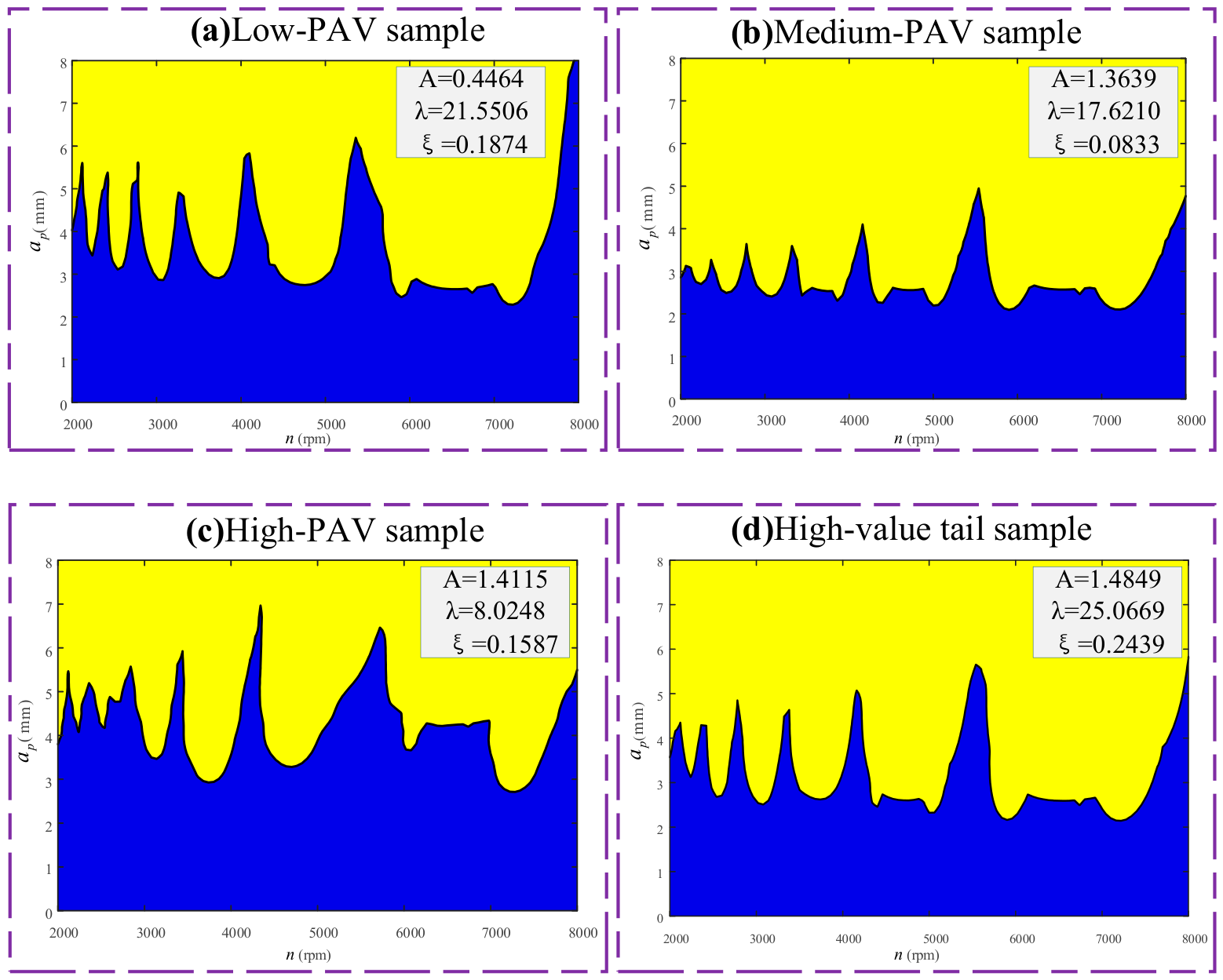
To further reveal the stability differences of the wave-edge milling system under representative PAV levels from the graphical perspective, four waveform-parameter cases were selected for comparative analysis of the stability lobe diagrams. The first three cases were selected from the formal 54-sample set and correspond to low-PAV, medium-PAV, and high-PAV representative conditions, respectively. In addition, according to the treatment of high-value tail samples described in Section 3.3, one sample with $V>0.06$ that is not included in the formal stratified statistics was selected as a supplementary extreme case to examine the boundary behavior of the correspondence between PAV and stability. The detailed parameter values and corresponding SRA results are listed in

Table 7. Representative waveform parameter cases and corresponding SRA values.

Case	Sample Type	A (mm)	$\mathit{\lambda }$ (mm)	ξ	PAV	SRA (rpm·m)
1	Low-PAV	0.4464	21.5506	0.1874	4.98843 × 10−3	17.292
2	Medium-PAV	1.3639	17.6210	0.0833	2.167192 × 10−2	22.710
3	High-PAV	1.4115	8.0248	0.1587	4.500057 × 10−2	25.932
4	High-value tail case	1.4849	25.0669	0.2439	6.271321 × 10−2	19.422

.

As can be seen from Figure 12, the stability lobe diagrams of the four representative cases exhibit clear differences in stable-region morphology and SRA values. When the sample changes from the low-PAV representative case to the medium-PAV representative case, the stable region is enlarged, and the SRA increases from 17.292 to 22.710, in units of $\mathrm{r}\mathrm{p}\mathrm{m}\cdot \mathrm{m}$. When the PAV further increases to the high-PAV representative case, the SRA reaches 25.932 $\mathrm{r}\mathrm{p}\mathrm{m}\cdot \mathrm{m}$. However, the high-value tail case with $V>0.06$, which is not included in the formal stratified statistics, has an SRA of 19.422 $\mathrm{r}\mathrm{p}\mathrm{m}\cdot \mathrm{m}$. Although its PAV is higher than those of the formal representative cases, its SRA is lower than those of the medium-PAV and high-PAV representative cases. The high-value tail case indicates that a higher PAV does not necessarily lead to better stability. Excessively high PAV may correspond to an unfavorable organization of local time delays or cutting-force distribution. Therefore, PAV should be interpreted together with the specific waveform-parameter combination, and final tool selection still requires SLD/SRA verification.

5.4. Mechanism and Applicability Boundaries of PAV as a Probability-Biased Screening Descriptor

Existing studies have focused on the trend consistency between PAV and SRA under controlled variations of waveform parameters. This study further investigates whether such trend consistency can be extended to a large-scale coupled parameter space in the form of probability-biased pre-screening, and where the applicability boundaries of PAV lie.

PAV is physically related to milling stability because it reflects the fluctuation intensity of local pitch angles and the corresponding diversity of inter-tooth time delays. In general, larger time-delay diversity is more conducive to weakening the continuous accumulation of the regenerative effect between adjacent teeth. This explains why higher-PAV layers tend to show larger mean SRA values and higher probabilities of containing large-SRA samples. However, chatter stability in milling is governed by the complete dynamic system rather than by delay variation alone. Previous studies on multi-delay and time-periodic milling dynamics have shown that stability boundaries are affected by modal dynamics, directional cutting-force coefficients, spindle speed, axial depth of cut, tool–workpiece engagement, and the spatial organization of local delays [24,25,26]. Therefore, the low pointwise R² value is not contradictory to the probability-biased screening role of PAV. Instead, it indicates that PAV cannot determine the SRA of an individual waveform-parameter set and should not be used as a stand-alone stability selection criterion.

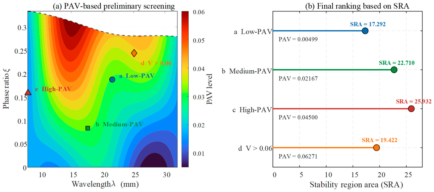
Figure 13 provides an intuitive illustration of the complementary roles of PAV and SLD/SRA in waveform-parameter screening. Figure 13a schematically shows that PAV can be used as a low-cost probability-biased descriptor to prioritize candidate regions with higher stability potential. Figure 13b further compares the final SRA ranking of representative cases. The high-PAV representative case achieves the largest SRA, whereas the high-value tail case does not obtain the highest stability despite having the largest PAV. Therefore, a more reasonable strategy for practical parameter optimization is to use PAV only for preliminary probability-biased pre-screening, followed by high-fidelity SLD/SRA evaluation for final stability ranking and tool selection.

6. Conclusions

This study investigated the relationship between pitch angle variance and milling stability under coupled waveform-parameter variations. A PAV-based stratified sampling and stability evaluation framework was established for wave-edge milling tools. The main conclusions are as follows:

(1)

A feasible waveform-parameter space was constructed under progressive phase distribution by considering manufacturing feasibility and wave-edge non-interference constraints. This provides a unified basis for PAV calculation, representative sample selection, and subsequent stability evaluation.

(2)

PAV was adopted to characterize the non-uniformity of local pitch angles and the corresponding diversity of inter-tooth time delays. The results indicate that PAV can reflect the time-delay fluctuation induced by waveform-parameter variations, but its role should be interpreted as a low-cost probability-biased descriptor rather than a deterministic stability predictor.

(3)

The PAV-based stratified sampling strategy reduced the number of high-fidelity SLD/SRA calculations from 2000 feasible waveform-parameter combinations to 54 representative samples, corresponding to a reduction of approximately 97.3% in the dominant stability-evaluation workload. Therefore, the proposed strategy can improve the efficiency of preliminary candidate-space reduction while retaining representative samples across different PAV levels.

(4)

The pointwise PAV–SRA relationship is weak under coupled waveform-parameter variations, with Pearson = 0.4234, Spearman = 0.4720, and R² = 0.179, indicating that PAV cannot deterministically predict the SRA of each individual parameter set. However, the stratified probability analysis shows that higher-PAV layers have a higher probability of producing large-SRA samples. The probability of obtaining an above-median SRA increases from 11.1% in Layer 1 to 88.9% in Layer 6, and the probability of obtaining an above-mean SRA increases from 11.1% to 77.8%.

(5)

The comparison of representative stability lobe diagrams further clarifies the applicability boundary of PAV. The SRA increases from 17.292 for the low-PAV representative case to 22.710 and 25.932 for the medium- and high-PAV representative cases, respectively, in units of $\mathrm{r}\mathrm{p}\mathrm{m}\cdot \mathrm{m}$. However, the high-value tail case with PAV > 0.06 rad² has a lower SRA of 19.422 $\mathrm{r}\mathrm{p}\mathrm{m}\cdot \mathrm{m}$, indicating that a higher PAV does not necessarily lead to better stability for an individual parameter set. Therefore, PAV should not be used as a stand-alone tool-selection criterion. It is more appropriate to use PAV as an auxiliary probabilistic pre-screening descriptor, while final tool selection still requires high-fidelity SLD/SRA verification.

In future work, representative low-, medium-, high-, and tail-PAV wave-edge tools will be fabricated and tested to further verify the experimental applicability of the proposed PAV-based pre-screening strategy. In addition, structural features characterizing the axial organization pattern of time delays can be introduced on the basis of PAV to construct a combined indicator or surrogate model integrating “PAV + distribution features”. By further combining this framework with high-fidelity stability solutions and experimental validation, a more efficient and reliable optimization method for wave-edge parameters can be developed.

References

1. Sellmeier, V.; Denkena, B. Stable Islands in the Stability Chart of Milling Processes Due to Unequal Tooth Pitch. Int. J. Mach. Tools Manuf. 2011, 51, 152–164. [Google Scholar] [CrossRef] [Scilit]
2. Suzuki, N.; Ishiguro, R.; Kojima, T. Design of Irregular Pitch End Mills to Attain Robust Suppression of Regenerative Chatter. CIRP Ann. 2016, 65, 129–132. [Google Scholar] [CrossRef] [Scilit]
3. Stepan, G.; Hajdu, D.; Iglesias, A.; Takacs, D.; Dombovari, Z. Ultimate Capability of Variable Pitch Milling Cutters. CIRP Ann. 2018, 67, 373–376. [Google Scholar] [CrossRef] [Scilit]
4. Mei, J.; Luo, M.; Guo, J.; Li, H.; Zhang, D. Analytical Modeling, Design and Performance Evaluation of Chatter-Free Milling Cutter with Alternating Pitch Variations. IEEE Access 2018, 6, 32367–32375. [Google Scholar] [CrossRef] [Scilit]
5. Comak, A.; Budak, E. Modeling Dynamics and Stability of Variable Pitch and Helix Milling Tools for Development of a Design Method to Maximize Chatter Stability. Precis. Eng. 2017, 47, 459–468. [Google Scholar] [CrossRef] [Scilit]
6. Zhan, D.; Jiang, S.; Niu, J.; Sun, Y. Dynamics Modeling and Stability Analysis of Five-Axis Ball-End Milling System with Variable Pitch Tools. Int. J. Mech. Sci. 2020, 182, 105774. [Google Scholar] [CrossRef] [Scilit]
7. Niu, J.; Ding, Y.; Zhu, L.; Ding, H. Mechanics and Multi-Regenerative Stability of Variable Pitch and Variable Helix Milling Tools Considering Runout. Int. J. Mach. Tools Manuf. 2017, 123, 129–145. [Google Scholar] [CrossRef] [Scilit]
8. Otto, A.; Rauh, S.; Ihlenfeldt, S.; Radons, G. Stability of Milling with Non-Uniform Pitch and Variable Helix Tools. Int. J. Adv. Manuf. Technol. 2017, 89, 2613–2625. [Google Scholar] [CrossRef] [Scilit]
9. Yusoff, A.R.; Sims, N.D. Optimisation of Variable Helix Tool Geometry for Regenerative Chatter Mitigation. Int. J. Mach. Tools Manuf. 2011, 51, 133–141. [Google Scholar] [CrossRef] [Scilit]
10. Guo, Y.; Lin, B.; Wang, W. Optimization of Variable Helix Cutter for Improving Chatter Stability. Int. J. Adv. Manuf. Technol. 2019, 104, 2553–2565. [Google Scholar] [CrossRef] [Scilit]
11. Li, M.; Zhao, W.; Li, L.; He, N. Investigation of Variable Pitch Tool Design for Chatter Suppression in Milling of Ti-6Al-4 V: A Comparison of Simulation and Experimental Results. Int. J. Adv. Manuf. Technol. 2022, 121, 3841–3855. [Google Scholar] [CrossRef] [Scilit]
12. Nie, W.; Zheng, M.; Zhang, W.; Liu, Y.; Bi, Y. Analytical Prediction of Chatter Stability with the Effect of Multiple Delays for Variable Pitch End Mills and Optimization of Pitch Parameters. Int. J. Adv. Manuf. Technol. 2023, 124, 2645–2658. [Google Scholar] [CrossRef] [Scilit]
13. Nie, W.; Zheng, M.; Yu, H.; Xu, S.; Liu, Y. Analysis of Vibration Reduction Mechanism for Variable Pitch End Mills. Int. J. Adv. Manuf. Technol. 2022, 119, 7787–7797. [Google Scholar] [CrossRef] [Scilit]
14. Ozsahin, O. Optimization of Variable Pitch Milling Tools for Improved Chatter Stability. J. Manuf. Process. 2024, 120, 260–271. [Google Scholar] [CrossRef] [Scilit]
15. Hu, X.; Qiao, H.; Yang, M.; Zhang, Y. Research on Milling Characteristics of Titanium Alloy TC4 with Variable Helical End Milling Cutter. Machines 2022, 10, 537. [Google Scholar] [CrossRef] [Scilit]
16. Sims, N.D.; Mann, B.; Huyanan, S. Analytical Prediction of Chatter Stability for Variable Pitch and Variable Helix Milling Tools. J. Sound Vib. 2008, 317, 664–686. [Google Scholar] [CrossRef] [Scilit]
17. Jiang, S.; Zhan, D.; Liu, Y.; Sun, Y.; Xu, J. Modeling of Variable-Pitch/Helix Milling System Considering Axially Varying Dynamics with Cutter Runout Offset and Tilt Effects. Mech. Syst. Signal Proc. 2022, 168, 108674. [Google Scholar] [CrossRef] [Scilit]
18. Tehranizadeh, F.; Berenji, K.R.; Yıldız, S.; Budak, E. Chatter Stability of Thin-Walled Part Machining Using Special End Mills. CIRP Ann. 2022, 71, 365–368. [Google Scholar] [CrossRef] [Scilit]
19. Yang, Y.; Liu, H.-L.; Yuan, J.-W.; Kong, W.-L.; Wan, M.; Zhang, W.-H. Development of an Anti-Vibration Cutting Tool Combining the Lattice Structures Infill with Damping Particles. Mech. Syst. Signal Process. 2025, 228, 112425. [Google Scholar] [CrossRef] [Scilit]
20. Jiang, S.; Qin, Z.; Chen, M.; Xu, J.; Sun, Y.; Deng, P. Explicit Geometry Framework Based Dynamic Modeling of Wave-Edge Milling and Stability Investigation on Waveform Parameters. J. Manuf. Process. 2025, 155, 1026–1048. [Google Scholar] [CrossRef] [Scilit]
21. Dombovari, Z.; Altintas, Y.; Stepan, G. The Effect of Serration on Mechanics and Stability of Milling Cutters. Int. J. Mach. Tools Manuf. 2010, 50, 511–520. [Google Scholar] [CrossRef] [Scilit]
22. Bari, P.; Law, M.; Wahi, P. Improved Chip Thickness Model for Serrated End Milling. CIRP J. Manuf. Sci. Technol. 2019, 25, 36–49. [Google Scholar] [CrossRef] [Scilit]
23. Sanz, M.; Iglesias, A.; Munoa, J.; Dombovari, Z. The Effect of Geometry on Harmonically Varied Helix Milling Tools. J. Manuf. Sci. Eng. 2020, 142, 074501. [Google Scholar] [CrossRef] [Scilit]
24. Bari, P.; Kilic, Z.M.; Law, M.; Wahi, P. Rapid Stability Analysis of Serrated End Mills Using Graphical-Frequency Domain Methods. Int. J. Mach. Tools Manuf. 2021, 171, 103805. [Google Scholar] [CrossRef] [Scilit]
25. Zhan, D.; Li, S.; Jiang, S.; Sun, Y. Optimal Pitch Angles Determination of Ball-End Cutter for Improving Five-Axis Milling Stability. J. Manuf. Process. 2022, 84, 832–846. [Google Scholar] [CrossRef] [Scilit]
26. Defant, F.; Ghezzi, D.; Albertelli, P. Development of a Generalized Extended Harmonic Solution for Analyzing the Combination of Chatter Suppression Techniques in Milling. J. Sound Vib. 2023, 543, 117368. [Google Scholar] [CrossRef] [Scilit]
Figure 1. Workflow of PAV-based probability-biased pre-screening and SLD/SRA-based stability evaluation.
Machines 14 00856 g001
Figure 2. Geometry and planar development of the cutting edges of the wave-edge milling tool: (a) three-dimensional geometry of the wave-edge milling tool; (b) planar development of the cutting edges with different phase parameters.
Machines 14 00856 g002
Figure 3. Distribution of geometric lag distances of different teeth along the axial depth.
Machines 14 00856 g003
Figure 4. Axial distributions of local pitch angles and their variances for representative parameter sets.
Machines 14 00856 g004
Figure 5. Feasible waveform-parameter space under geometric constraints: (a) feasible samples in the A λ ξ space; (b) projection in the λ ξ plane showing the feasible region and the excluded region with Δ l > 8   m m .
Machines 14 00856 g005
Figure 6. Statistical distribution of PAV in the feasible waveform-parameter space: (a) frequency distribution of PAV; (b) projected distribution of PAV in the wavelength–phase-ratio parameter plane.
Machines 14 00856 g006
Figure 7. Projection distribution of the 54 representative samples in the wavelength–phase-ratio parameter plane.
Machines 14 00856 g007
Figure 8. Global correspondence between PAV and SRA for the 54 representative samples: (a) PAV–SRA scatter plot with linear fitting; (b) stratified distribution of samples in the PAV–SRA plane.
Machines 14 00856 g008
Figure 9. Comparison of the variation trends of normalized PAV and normalized SRA after sorting by PAV.
Machines 14 00856 g009
Figure 10. Stratified statistical analysis of SRA for the 54 representative samples: (a) distribution of SRA in each PAV layer; (b) mean SRA and standard deviation of each PAV layer; (c) trend of mean SRA across PAV layers.
Machines 14 00856 g010
Figure 11. Nonparametric pairwise comparison of SRA distributions among different PAV layers: (a) pairwise p-value matrix based on the Mann–Whitney U test; (b) effect size matrix based on Cliff’s delta.
Machines 14 00856 g011
Figure 12. Comparison of stability lobe diagrams for representative waveform-parameter cases: (a) low-PAV representative case; (b) medium-PAV representative case; (c) high-PAV representative case; (d) high-value tail case with V > 0.06 . The blue and yellow areas indicate the stable and unstable milling regions, respectively.
Machines 14 00856 g012
Figure 13. Schematic illustration of PAV-based probability-biased pre-screening and final SRA-based stability ranking: (a) PAV-based pre-screening map in the wavelength–phase-ratio parameter plane; (b) final ranking of representative cases based on SRA.
Machines 14 00856 g013