Multiple Frequency Vibration Estimation in Controlled Electric Synchronous Motor Systems

Abstract

Synchronous motors are widely used in applications demanding high efficiency, torque density, and precise velocity regulation, such as electrified transportation, industrial automation, and robotics. Their operation, however, is degraded by mechanical and electromagnetic disturbances that induce oscillatory load torque components, worsening velocity tracking and increasing mechanical stress. This paper presents a control-based reconstruction and harmonic characterization framework for multiple-frequency load torque disturbances in permanent magnet synchronous motor systems, addressing the order-based case in which the harmonic frequencies scale with the rotor speed. The proposed approach combines a robust velocity tracking control structure with a disturbance torque reconstruction scheme based on internal signals of the control system, so that the estimated torque acts as a virtual sensor. The reconstructed disturbance is resampled in the angular domain, where each speed order becomes stationary, and is processed by a hybrid Empirical–Variational mode decomposition with a blind order-identification stage; the Hilbert transform then yields the amplitude, frequency, and phase of each component without prior knowledge of the orders present. Unlike approaches based on additional sensors, specific harmonic observers, or detailed disturbance models, the proposed methodology relies solely on information already available within the control structure. The framework is validated on a surface-mounted and salient-pole permanent magnet synchronous motor under speed-dependent multiple-frequency disturbances, including a nonstationary Bézier load profile with amplitude-modulated harmonics, and remains reliable under measurement noise and abrupt load-torque steps. The yielded results evidence the proposed framework represents an efficient approach for condition monitoring, fault diagnosis, and predictive maintenance by accurate velocity tracking, adequate disturbance torque reconstruction, and precise harmonic characterization in synchronous-motor drive systems.

1. Introduction

Electric drives based on synchronous machines are used in several modern engineering applications due to their high efficiency and accurate torque, speed, and position regulation [1,2]. They are commonly found in robotic systems, precision motion platforms, renewable energy converters, electric vehicles, and automated production processes [2,3]. However, their performance may be affected by parameter variations, unmodeled dynamics, and external disturbances. Consequently, suitable estimation and control techniques are required to preserve the desired operating conditions [4,5].

Continuous advances and innovations in machine topology continue to improve the performance of these drives, with recent designs achieving higher torque density, greater efficiency, and better magnet utilization, while also improving the quality of the generated torque. For instance, partitioned-stator flux-switching machines exploiting a strongly coupled flux-reversal effect achieve higher average torque with reduced torque ripple [6], whereas hybrid-magnet multilayer interior permanent magnet motors employing fractional-slot windings and flux-barrier structures suppress cogging torque to enable low-vibration operation in cost- and supply-constrained traction applications [7]. These advances confirm that torque ripple and vibration remain central design concerns even in state-of-the-art synchronous machines, reinforcing the need for the accurate characterization of the oscillatory load torque addressed in this work.

These type of electromechanical systems may be subjected to undesired mechanical and electromagnetic vibrations which deteriorate significantly their performance. These undesired oscillations may arise from a wide variety of sources including structural resonances, unbalanced loads, shaft misalignments, bearing irregularities, power electronic switching effects, cogging torque, torque ripple, and interactions with external mechanical components [8,9,10]. Without a proper treatment, such perturbations lead to degraded tracking accuracy, increased mechanical stress, higher acoustic noise levels, excessive current demand, and reduced operational lifetime of the machinery [9,11].

For these reasons, the analysis, estimation, and possible suppression of vibrations in rotating electrical machines have become central objectives in modern motion control engineering. Active vibration control techniques have been widely investigated as an effective means to counteract oscillatory disturbances in real time, providing several advantages over purely passive damping approaches [8,12]. The main drawback for vibration attenuation or compensation schemes is the necessity for detailed knowledge of the disturbances features such as the amplitude, frequency, and phase of the oscillatory components, which are essential for understanding the origin, intensity, and temporal behavior of the load torque vibrations.

Under industrial operating conditions, vibrations rarely remain constant or are fully known beforehand. Their amplitude, frequency, and phase change with the operating point, load profile, mechanical coupling, and component wear. Reliable estimation of these parameters is therefore needed for drive operation, condition monitoring, fault detection, and predictive maintenance in synchronous motor systems [13,14]. Deficient estimation can also reduce the performance of vibration monitoring and suppression methods.

Among the different parameters describing oscillatory phenomena, identification of vibration frequencies is of particular importance. Frequency information enables the design of selective filters, adaptive compensation mechanisms, and diagnostic tools aimed at mitigating or identifying specific harmonic components [15,16]. Moreover, knowledge of dominant oscillation modes can be directly exploited for online condition monitoring, predictive maintenance, and detection of abnormal operating conditions [2,17].

A variety of strategies have been proposed to estimate and attenuate such multiperiodic disturbances. Extended Kalman filters have been employed to reconstruct periodic load torque components and reduce velocity ripple in PMSM drives [18]; adaptive periodic estimators have been embedded into disturbance-rejection current controllers [19]; identified vibration models have enabled multi-frequency vibration suppression in multiphase machines [20]; and adaptive observer and internal-model approaches based on output regulation can reject multi-frequency sinusoidal load torques even when only an upper bound on the number of harmonics is known [21].

These contributions show that estimating multiple oscillatory components is an active and, in several settings, effectively addressed problem. Nevertheless, most of these techniques rely on a detailed dynamic model of the machine, require a nontrivial observer or filter design, assume prior knowledge of the disturbance structure, or are oriented towards disturbance rejection rather than the explicit characterization of each individual harmonic component. Consequently, the development of methodologies able to provide model-independent harmonic characterization of load torque disturbances, reconstructing the amplitude, frequency, and phase of each component directly from signals already available within the control loop, while simultaneously preserving high-performance velocity regulation remains a relevant open research challenge.

From a motion control perspective, addressing these challenges requires strategies capable of maintaining accurate velocity tracking under uncertain and time-varying conditions. In this context, the design of high-performance velocity control systems for synchronous motors has been an active research topic for several decades. PI and PID controllers, linear observers, and model-based compensation methods remain common choices for synchronous motor drives [22,23]. Their simple structure and moderated computational burden facilitate real-time implementation, however, is sensitive to modeling errors and controller tuning, particularly when nonlinear effects, parameter variations, and external disturbances are present [24,25].

During operation synchronous motor drives are frequently affected by time-varying loads, unmodeled dynamics, and mechanical vibrations that degrade velocity tracking performance. Traditional linear control schemes exhibit limited robustness against such perturbations and often require extensive retuning when operating conditions change [19,26]. To overcome these limitations, advanced nonlinear and robust control techniques have been investigated, including sliding-mode control, backstepping, model predictive control, disturbance rejection control, and adaptive robust controllers [27,28].

Although these methods improve disturbance rejection, many require detailed system models and complex design procedures, which may limit real-time implementation [5,23]. To reduce this dependence, feedback structures incorporating automatic tuning have been proposed, such as auto-tuned constrained state-feedback controllers whose gains are adjusted online by nature-inspired optimization to attenuate periodic disturbances without an explicit disturbance model [29]. However, such schemes remain primarily devoted to disturbance attenuation and do not provide an explicit, per-component characterization of the oscillatory load torque.

Classical vibration estimation techniques including Fourier-based spectral analysis, adaptive notch filters, phase-locked loops, and observer-based methods [9,15] have been applied to estimate oscillations affecting electric drives. Although these techniques perform well in specific applications, their integration into velocity control systems subject to nonstationary multifrequency disturbances remains challenging. Most require predefined frequency ranges, assume quasi-stationary conditions, or rely on detailed knowledge of the system dynamics, which limits their use under uncertain operating conditions [2,9]. In addition, Fourier-based approaches provide global spectral information but may lose temporal resolution when the disturbance signal contains nonstationary components or amplitude variations.

The Hilbert–Huang transform and Empirical Mode Decomposition (EMD) are commonly considered for nonstationary vibration signals in electrical and mechanical systems [9,30]. Throughout the decomposition procedure, the measured response is separated into intrinsic mode functions directly from the data, so neither a predefined harmonic basis nor a stationary representation is imposed. Each extracted component describes part of the local oscillatory content and can be examined over time. In practice, however, the decomposition is sensitive to noise and mode mixing, and its mathematical basis is less formal than that of optimization-based methods. These issues are particularly important when the signal contains closely spaced frequencies or when the algorithm must operate within a real-time control scheme [30,31,32].

Variational Mode Decomposition (VMD) is formulated to separate a multicomponent signal into a fixed number of band-limited modes [32,33,34]. Unlike empirical decomposition procedures, the number of modes is selected beforehand and each component is obtained around a specific center frequency. This formulation can reduce sensitivity to noise and avoid some numerical difficulties associated with empirical techniques [32,33,34,35]. For this reason, variational mode decomposition has been considered for harmonic estimation in rotating machinery and electric drive applications.

Despite these advantages, the direct application of this technique may require an adequate selection of decomposition parameters and the number of modes, which is not always straightforward when the disturbance signal contains both stationary and nonstationary components. Therefore, the combination of variational and empirical mode decomposition represents a suitable alternative for exploiting the spectral separation advantages of the variational technique while incorporating the adaptive decomposition capability of the empirical technique.

Once the oscillatory modes have been separated, the extraction of harmonic parameters is necessary for a complete description of the disturbance signal. In this context, the Hilbert transform provides a useful tool for constructing the analytic signal associated with each extracted mode, allowing the estimation of the instantaneous amplitude, frequency, and phase. These quantities provide a detailed characterization of the dynamic behavior of each vibration component and make it possible to analyze how the disturbance evolves over time. For synchronous motor systems, this information can be used to identify dominant vibration modes, evaluate the quality of the reconstructed load torque signal, and provide useful indicators for condition monitoring and predictive maintenance.

The literature reveals two main limitations. Many vibration estimation methods rely on accelerometers, torque sensors, or dedicated monitoring equipment, increasing implementation cost and system complexity. Other techniques require accurate mathematical models, prior knowledge of the disturbance, or predefined spectral ranges. Although the signals available in the speed control loop contain information about the load torque acting on the motor shaft, they have not been fully used to reconstruct and characterize its multifrequency vibration components without additional sensors or prior spectral information. These limitations show that reconstructing and characterizing multifrequency load torque vibrations from the velocity control-loop signals remains an unresolved problem.

This paper proposes a reconstruction and harmonic characterization framework based on control signals for multiple-frequency load torque vibrations in permanent magnet synchronous motor (PMSM) systems. The proposed scheme reconstructs the disturbance torque from available signals in the velocity control loop and extracts its harmonic content using a hybrid Empirical–Variational mode decomposition strategy. Next, the Hilbert transform is applied to the oscillatory modes extracted from the reconstructed disturbance signal to estimate the amplitude, frequency, and phase of each harmonic component. Unlike methods that depend on additional sensors, dedicated harmonic observers, detailed disturbance models, or machine-learning techniques, this approach relies only on signals available in the control loop.

The proposed framework allows the characterization of multiple stationary and nonstationary harmonic components acting on the motor shaft, while simultaneously performing a proper velocity reference tracking. The framework offers several practical advantages, including the reconstruction of the load torque disturbance from internal control-related signals, model-independent harmonic analysis of the disturbance, the separation of multiple oscillatory modes via hybrid Empirical–Variational mode decomposition processing, and the extraction of instantaneous harmonic parameters through the Hilbert transform. Although the present study focuses on permanent magnet synchronous motors, the proposed estimation framework can be extended to other electrical machines and nonlinear electromechanical systems affected by uncertain oscillatory load disturbances.

The remainder of this paper is organized as follows: Section 2 presents the mathematical formulation of the permanent magnet synchronous motor system as well as the load torque disturbance model in the presence of unknown oscillatory components. In Section 3, the velocity tracking control structure and the reconstruction of the disturbance torque signal from internal control dynamics are described. The hybrid Empirical–Variational mode decomposition technique for vibration estimation and explains the extraction of harmonic parameters through the Hilbert transform is introduced in Section 4. Section 5 presents the analytical and numerical validation of the proposed approach under several operating conditions with multiple-frequency disturbances. Finally, Section 6 summarizes the main conclusions and outlines some directions for future research and applications.

2. Mathematical Model of the Permanent Magnet Synchronous Motor

As illustrated in Figure 1, the physical structure of a permanent magnet synchronous motors consist of a stator with three-phase windings and a rotor equipped with permanent magnets. The interaction between the stator currents and the rotor magnetic field generates the electromagnetic torque that drives the mechanical shaft, whereas the rotor dynamics are influenced by the external load torque and possible oscillatory disturbances [36].

Nonlinear dynamics in the $dq$ reference frame of a permanent magnet synchronous motor can be described in state space by

$$\begin{array}{c}\hfill {\displaystyle \frac{d}{dt}}z=f(z,v,{\tau }_L),z\left(t_0\right)=z_0,z\in {\mathbb{R}}^3,\end{array}$$

(1)

with

$$f(z,v,{\tau }_L)=\left[\begin{array}{c}{\displaystyle \frac{3}{2J}}{n}_p\left[{\lambda }_m+\left(L_d-L_q\right)i_d\right]i_q-{\displaystyle \frac{b}{J}}\omega -{\displaystyle \frac{1}{J}}{\tau }_L\\ -{\displaystyle \frac{R_s}{L_q}}{i}_q-{\displaystyle \frac{L_d{n}_p}{L_q}}{i}_d\omega -{\displaystyle \frac{n_p{\lambda }_m}{L_q}}\omega +{\displaystyle \frac{1}{L_q}}{v}_q\\ -{\displaystyle \frac{R_s}{L_d}}{i}_d+{\displaystyle \frac{L_q{n}_p}{L_d}}{i}_q\omega +{\displaystyle \frac{1}{L_d}}{v}_d\end{array}\right].$$

(2)

The state vector is denoted as $z={[\omega ,i_q,i_d]}^T$, where $\omega$ refers to the rotor speed, $i_q$ expresses the quadrature current and $i_d$ corresponds to the direct current. The voltage input vector is represented as $v={[v_q,v_d]}^T$, where $v_q$ is the quadrature voltage and $v_d$ is the direct voltage. Quadrature and direct inductances are defined as $L_q$ and $L_d$. $R_s$ stands for the stator resistance, $n_p$ specifies the number of pole pairs and ${\lambda }_m$ indicates the magnetic flux of permanent magnet. J represents the equivalent inertia and b symbolizes the viscous damping both of the rotational mechanical system.

The control electromagnetic torque ${\tau }_u$ generated by the electric motor is given by

$${\tau }_u={\displaystyle \frac{3}{2}}{n}_p\left[{\lambda }_m+\left(L_d-L_q\right)i_d\right]i_q.$$

(3)

In this expression, the first term corresponds to the magnetic alignment torque produced by the permanent-magnet flux ${\lambda }_m$, whereas the second term represents the reluctance torque associated with the magnetic saliency $L_d\ne L_q$. The reluctance contribution is exploited when a nonzero direct-axis current $i_d$ is imposed.

Dynamics of the load torque ${\tau }_L$ of the rotational mechanical system coupled to the rotor of the motor with undesirable arbitrary frequency vibration components is described as

$$\begin{array}{c}\hfill {\tau }_L={\tilde{\tau }}_L+{\displaystyle \sum _{j=1}^m}{\tau }_{L,j}cos\left({\theta }_{L,j}-{\phi }_{L,j}\right),{\theta }_{L,j}={\int }_{t_0}^t{\mathrm{\Omega }}_{L,j}\left(s\right)\mathrm{d}s.\end{array}$$

(4)

Here, ${\tau }_{L,j}$, ${\mathrm{\Omega }}_{L,j}$ and ${\phi }_{L,j}$ denote, respectively, the possibly time-varying amplitude, the instantaneous angular frequency, and the initial phase of the j-th vibration component, while ${\theta }_{L,j}$ is its instantaneous phase. Expressing the argument through the instantaneous phase ${\theta }_{L,j}$, rather than through a fixed term ${\mathrm{\Omega }}_{L,j}t$, allows the model to represent both stationary and nonstationary oscillatory disturbances, and is consistent with the instantaneous-frequency description recovered by the Hilbert-transform stage in Section 4, where ${\mathrm{\Omega }}_{L,j}=\mathrm{d}{\theta }_{L,j}/\mathrm{d}t$.

In rotating electrical machines, oscillatory load torque components could not occur at fixed frequencies but at integer multiples of the rotational speed, referred to as speed orders. Mechanisms such as cogging torque, flux-harmonic distortion, rotor eccentricity, gear meshing, and mass unbalance produce harmonics whose frequencies scale with the operating speed, so that

$${\mathrm{\Omega }}_{L,j}=h_j\omega ,$$

(5)

where $h_j$ is the characteristic order of the j-th component with respect to the mechanical rotational speed $\omega$; for electromagnetically induced harmonics, $h_j$ is a multiple of the pole-pair number $n_p$, i.e., referred to the electrical angular frequency ${\omega }_e=n_p\omega$. Other disturbance sources, such as structural resonances or inverter switching effects, are essentially independent of the rotational speed and are recovered as the particular case of constant ${\mathrm{\Omega }}_{L,j}$. Parametric variations in the amplitudes and frequencies are thus admitted by the model, and other deterministic or slowly varying load profiles are represented by ${\tilde{\tau }}_L$.

Nevertheless, arbitrary and unknown frequencies of completely uncertain oscillatory components can be also considered, in accordance with the application of the electric motor used as a motion actuator in some engineering system under influence of load torque vibrations.

3. Velocity Tracking Control Formulation

For control design, ${\tau }_L$ is modelled within an adaptive small interval of time around time $t_i$ as

$${\tau }_L={\displaystyle \sum _{k=0}^n}{\tau }_{k,t_i}{\left(t-t_i\right)}^k,t_i\le t\le t_i+ϵ.$$

(6)

Moreover, the parameters ${\tau }_{k,t_i}$ are assumed to be unknown and $ϵ>0$. In this fashion, the capability to suppress exogenous vibrations with uncertain multiple-frequency components is incorporated into the electromagnetic torque controller ${\tau }_u$. The order n of the polynomial approximation in Equation (6) is selected according to the expected complexity of the disturbance profile and the desired robustness of the control structure.

On each small time window $[t_i,t_i+ϵ]$, the load torque disturbance admits the local polynomial description presented in Equation (6) with unknown but bounded coefficients ${\tau }_{k,t_i}$; equivalently, ${\tau }_L$ is sufficiently smooth for its $(n+1)$-th time derivative to be negligible over the window. This family captures constant, ramp and polynomial loads, as well as the slowly varying envelopes and the locally band-limited oscillatory components introduced in Section 2. It constitutes the only structural assumption required by the proposed design: neither an exact disturbance model, nor its frequency content, nor additional sensors are needed, which is what enables the model-independent reconstruction in this work.

The tracking error of the desired speed profile is $e_{\omega }:=\omega -{\omega }^{\star }$. A dynamic torque controller can then be derived from Equations (1) and (6) to achieve robust tracking of the reference speed trajectory ${\omega }^{\star }$, as expressed in Equation (7).

$${\tau }_u=J{\displaystyle \frac{d}{dt}}{\omega }^{\star }+b{\omega }^{\star }-{\beta }_{n+1,{\tau }_u}{e}_{\omega }-{\tau }_{u_1}.$$

(7)

with

$$\begin{array}{cc}\hfill {\displaystyle \frac{d}{dt}}{\tau }_{u_1}=& {\beta }_{n,{\tau }_u}{e}_{\omega }+{\tau }_{u_2},\hfill \\ \hfill {\displaystyle \frac{d}{dt}}{\tau }_{u_2}=& {\beta }_{n-1,{\tau }_u}{e}_{\omega }+{\tau }_{u_3},\hfill \\ \hfill & ⋮\hfill \\ \hfill {\displaystyle \frac{d}{dt}}{\tau }_{u_{n-1}}=& {\beta }_{2,{\tau }_u}{e}_{\omega }+{\tau }_{u_n},\hfill \\ \hfill {\displaystyle \frac{d}{dt}}{\tau }_{u_n}=& {\beta }_{1,{\tau }_u}{e}_{\omega }+{\tau }_{u_{n+1}},\hfill \\ \hfill {\displaystyle \frac{d}{dt}}{\tau }_{u_{n+1}}=& {\beta }_{0,{\tau }_u}{e}_{\omega }.\hfill \end{array}$$

(8)

The auxiliary variables ${\tau }_{u_1},\dots ,{\tau }_{u_{n+1}}$ defined in Equation (8) are not physical state variables of the motor but extended state variables of an Extended Proportional–Integral compensator [37]. Driven by the tracking error $e_{\omega }$, this cascade of integrators embeds an internal model of the disturbance; it asymptotically reproduces the unknown load torque together with its successive time derivatives, so that the first state variable provides an online estimate of the disturbance, i.e., ${\tau }_{u_1}\to -{\tau }_L$. The controller therefore rejects and simultaneously reconstructs ${\tau }_L$ from the tracking error, without measuring or modeling it explicitly.

The quadrature reference current signal $i_q^{\star }$ can be hence computed as

$$i_q^{\star }={\displaystyle \frac{2}{3}}{\displaystyle \frac{1}{n_p\left[{\lambda }_m+\left(L_d-L_q\right)i_d\right]}}{\tau }_u.$$

(9)

The design parameters ${\beta }_{j,{\tau }_u}>0$, $j=0,1,\dots ,n+1$, should be therefore determined so that the closed-loop dynamics of the tracking error

$$\left[J{\displaystyle \frac{d^{n+2}}{d{t}^{n+2}}}+\left(b+{\beta }_{n+1,{\tau }_u}\right){\displaystyle \frac{d^{n+1}}{d{t}^{n+1}}}+\dots +{\beta }_{1,{\tau }_u}{\displaystyle \frac{d}{dt}}+{\beta }_{0,{\tau }_u}\right]e_{\omega }=0$$

(10)

is exponentially stable.

A systematic and reproducible selection of the gains ${\beta }_{j,{\tau }_u}$ follows from imposing a single desired closed-loop bandwidth on Equation (10). Placing all roots of the associated monic characteristic polynomial at a common value $-{\alpha }_{\omega }$, with ${\alpha }_{\omega }>0$, gives

$$s^{n+2}+{\displaystyle \frac{b+{\beta }_{n+1,{\tau }_u}}{J}}{s}^{n+1}+\dots +{\displaystyle \frac{{\beta }_{1,{\tau }_u}}{J}}s+{\displaystyle \frac{{\beta }_{0,{\tau }_u}}{J}}={\left(s+{\alpha }_{\omega }\right)}^{n+2},$$

(11)

from which the gains are obtained in closed form as the scaled binomial coefficients ${\beta }_{n+1,{\tau }_u}=(n+2)J{\alpha }_{\omega }-b$ and ${\beta }_{m,{\tau }_u}=J\left({\displaystyle \genfrac{}{}{0pt}{}{n+2}{n+2-m}}\right){\alpha }_{\omega }^{n+2-m}$, $m=0,\dots ,n$. Since the resulting polynomial is Hurwitz by construction, the tracking error $e_{\omega }$ and the reconstruction error ${\tau }_{u_1}+{\tau }_L$ converge exponentially to a small residual set whose size is governed by the neglected $(n+1)$-th derivative of ${\tau }_L$. The single parameter ${\alpha }_{\omega }$ thus fixes the convergence rate of both objectives, trading faster disturbance rejection and tracking against increased measurement-noise sensitivity and control effort.

As a result, the speed tracking error dynamics under the influence of load torque vibrations are described in Equation (12):

$$J{\displaystyle \frac{d}{dt}}{e}_{\omega }+\left(b+{\beta }_{n+1,{\tau }_u}\right)e_{\omega }=-{\tau }_{u_1}-{\tau }_L.$$

(12)

Based on Equation (12), the internal dynamic compensation signal ${\tau }_{u_1}$ contains information associated with the unknown load torque disturbance. Therefore, the dynamic load torque can be directly estimated from the control structure as expressed in Equation (13):

$${\widehat{\tau }}_L\approx -{\tau }_{u_1}.$$

(13)

Controllers for tracking of quadrature and direct current reference trajectories, $i_q^{\star }$ and $i_d^{\star }$, with capabilities to suppress possible dynamic disturbances are proposed as follows:

$$\begin{array}{cc}\hfill v_q=& L_q{\displaystyle \frac{d}{dt}}{i}_q^{\star }+R_s{i}_q^{\star }+n_p{L}_d{i}_d\omega +n_p{\lambda }_m\omega -{\beta }_{n_q+1,v_q}{e}_{i_q}-v_{q_1},\hfill \\ \hfill v_d=& L_d{\displaystyle \frac{d}{dt}}{i}_d^{\star }+R_s{i}_d^{\star }-n_p{L}_q{i}_q\omega -{\beta }_{n_d+1,v_d}{e}_{i_d}-v_{d_1},\hfill \end{array}$$

(14)

with

$$\begin{array}{cc}\hfill {\displaystyle \frac{d}{dt}}{v}_{{\rho }_1}=& {\beta }_{n_{\rho },v_{\rho }}{e}_{i_{\rho }}+v_{{\rho }_2},\hfill \\ \hfill {\displaystyle \frac{d}{dt}}{v}_{{\rho }_2}=& {\beta }_{n_{\rho }-1,v_{\rho }}{e}_{i_{\rho }}+v_{{\rho }_3},\hfill \\ \hfill & ⋮\hfill \\ \hfill {\displaystyle \frac{d}{dt}}{v}_{{\rho }_{n_{\rho }-1}}=& {\beta }_{2,v_{\rho }}{e}_{i_{\rho }}+v_{{\rho }_{n_{\rho }}},\hfill \\ \hfill {\displaystyle \frac{d}{dt}}{v}_{{\rho }_{n_{\rho }}}=& {\beta }_{1,v_{\rho }}{e}_{i_{\rho }}+v_{{\rho }_{n_{\rho }+1}},\hfill \\ \hfill {\displaystyle \frac{d}{dt}}{v}_{{\rho }_{n_{\rho }+1}}=& {\beta }_{0,v_{\rho }}{e}_{i_{\rho }}.\hfill \end{array}$$

(15)

Closed-loop dynamics of current reference tracking errors, $e_{\rho }:=i_{\rho }-i_{\rho }^{\star }$, $\rho =q,d$, are then described by

$$L_{\rho }{\displaystyle \frac{d}{dt}}{e}_{i_{\rho }}+\left(R_s+{\beta }_{n_{\rho }+1,v_{\rho }}\right)e_{i_{\rho }}=-v_{{\rho }_1}.$$

(16)

For applications in which the quadrature- and direct-axis current dynamics are not affected by significant disturbances, exponential stability of the tracking errors can be achieved by selecting positive gains, ${\beta }_{n_{\rho }+1,v_{\rho }}>0$, and setting $v_{{\rho }_1}=0$. Conversely, for significantly perturbed electric current dynamics, controllers with dynamic disturbance compensators, as defined in Equation (15), are proposed. As a consequence, disturbances similar to those described by Equation (6) can be suppressed. In this sense, the order of the corresponding polynomial expansions for the quadrature- and direct-axis current disturbances is represented by $n_{\rho }$.

The closed-loop dynamics of the quadrature- and direct-axis currents under the controllers defined in Equation (14) are then described by

$$\left[L_{\rho }{\displaystyle \frac{d^{n_{\rho }+2}}{d{t}^{n_{\rho }+2}}}+\left(R_s+{\beta }_{n_{\rho }+1,v_{\rho }}\right){\displaystyle \frac{d^{n_{\rho }+1}}{d{t}^{n_{\rho }+1}}}+\dots +{\beta }_{1,v_{\rho }}{\displaystyle \frac{d}{dt}}+{\beta }_{0,v_{\rho }}\right]e_{\rho }=0.$$

(17)

Control parameters ${\beta }_{0,v_{\rho }},{\beta }_{1,v_{\rho }},\dots ,{\beta }_{n_{\rho }+1,v_{\rho }}$ should be properly computed to get exponential stability of tracking errors $e_{\rho }$, $\rho =q,d$.

The same rationale applies to the inner current loops. In the disturbance-free case, setting $v_{{\rho }_1}=0$ reduces Equation (16) to first-order exponentially stable error dynamics, whereas the extended compensators of Equation (15) are activated only when the current dynamics are significantly perturbed, reconstructing the corresponding disturbance exactly as in the velocity loop. Their gains ${\beta }_{j,v_{\rho }}$ are selected by the same placement rule, matching the monic form of Equation (17) to ${\left(s+{\alpha }_{\rho }\right)}^{n_{\rho }+2}$ with ${\alpha }_{\rho }>0$, $\rho =q,d$. The whole cascade is governed by only three design parameters, ${\alpha }_{\omega }$, ${\alpha }_q$ and ${\alpha }_d$, chosen so that the current loops are markedly faster than the velocity loop, thereby guaranteeing the time-scale separation required for the cascade to behave as designed.

4. Hybrid Vibration Estimation Method

The vibration estimation stage operates on the disturbance-related signal obtained from the control structure. As established in Section 3, the load torque disturbance is reconstructed from the internal control signal according to Equation (13). The reconstructed disturbance signal ${\widehat{\tau }}_L$ thus constitutes the input to the vibration estimation stage and the internal control structure provides information about the oscillatory disturbances affecting the motor shaft without requiring additional measurement devices.

The identification of the harmonic parameters associated with the oscillatory components acting on the motor shaft is achieved through the proposed approach. To this end, a hybrid signal decomposition strategy combining Empirical and Variational mode decomposition is adopted. This approach exploits the adaptive properties of empirical technique incorporating the enhanced spectral separation capabilities of variational technique, enabling accurate estimation even in the presence of closely spaced frequency components.

4.1. Empirical Mode Decomposition

The empirical mode decomposition is a data-driven method designed to analyze nonlinear and non-stationary signals by decomposing them into intrinsic mode functions [38,39]. After applying the empirical mode decomposition to the reconstructed perturbation signal ${\widehat{\tau }}_L$ the following equation is obtained:

$${\widehat{\tau }}_L={\displaystyle \sum _{i=1}^m}{\mathrm{IMF}}_i+r,$$

(18)

where ${\mathrm{IMF}}_i$ denotes the i-th intrinsic mode function and r represents the residual trend.

Each intrinsic mode function satisfies two fundamental conditions: the first is the number of extrema and zero crossings differ by at most one, and the second is related to the local mean value is approximately zero. These conditions ensure that each intrinsic mode function represents a narrow-band oscillatory component.

Nevertheless, the adaptive nature of empirical mode decomposition makes it susceptible to mode mixing when oscillatory components with closely spaced frequencies coexist or when amplitude modulation is present. Under such conditions, a single intrinsic mode function may contain multiple frequency components, or a single component may be distributed across different intrinsic mode functions, degrading the accuracy of harmonic parameter identification. To overcome this limitation, variational mode decomposition is incorporated as a refinement stage [33].

4.2. Variational Mode Decomposition Refinement

The variational technique consists of decomposing a signal into a predefined number of band-limited modes by solving the next constrained variational problem

$$\underset{\left\{u_k\right\},\left\{{\omega }_k\right\}}{min}\left\{{\displaystyle \sum _{k=1}^K}{∥{\partial }_t\left[\left(\delta +{\displaystyle \frac{j}{\pi t}}\right)⁎u_k\right]e^{-j{\omega }_{k}t}∥}_2^2\right\},$$

(19)

subject to the reconstruction constraint defined as

$${\displaystyle \sum _{k=1}^K}{u}_k={\widehat{\tau }}_L,$$

(20)

where $u_k$ represents the k-th variational mode and ${\omega }_k$ the estimated center frequency. By solving equations in (19) and (20) provides modes with compact and well-separated spectral support, allowing for the handling of closely spaced frequency components that EMD fails to solve properly.

4.3. Hybrid Decomposition Strategy

The hybrid methodology combines the adaptability of EMD with the spectral resolution of VMD through a suitably activation mechanism and a preprocessing step [32]. The procedure is structured into the stages described below.

First, the presence of significant oscillatory components in ${\widehat{\tau }}_L$ is evaluated through the energy-based condition

$$\parallel {\widehat{\tau }}_L{\parallel }_2>\epsilon ,$$

(21)

where $\epsilon$ represents a predefined threshold. If the condition is not met, the signal is considered free of oscillatory disturbances and then the estimation stage is not activated.

If a significant disturbance is detected, EMD is applied to ${\widehat{\tau }}_L$ to obtain a preliminary set of intrinsic mode functions that reveal the dominant oscillatory patterns of the disturbance signal. The frequency proximity between adjacent modes is then evaluated as follows:

$$\Delta f_{ij}=|f_i-f_j|<{\delta }_f,$$

(22)

where $f_i$ and $f_j$ denote the dominant frequencies of the i-th and j-th intrinsic mode function, respectively, and ${\delta }_f$ is the spectral proximity threshold. In addition, the spectral overlap index is defined as

$${\mathcal{O}}_{ij}={\displaystyle \frac{{\displaystyle \int S_i\left(f\right)S_j\left(f\right)df}}{{\parallel S_i\parallel }_2{\parallel S_j\parallel }_2}},$$

(23)

where $S_i\left(f\right)$ and $S_j\left(f\right)$ are the power spectra of the i-th and j-th intrinsic mode function, respectively.

When the index ${\mathcal{O}}_{ij}$ exceeds the predefined threshold, a potential mode mixing is detected, and the VMD technique is applied to improve the decomposition. Otherwise, the Intrinsic Mode Functions obtained directly via EMD are accepted. This preprocessing mechanism reduces computational cost when EMD provides adequate spectral separation, reserving VMD for cases where robust resolution is strictly necessary.

If refinement is required, the number of variational modes is not set arbitrarily but is estimated from the preliminary empirical decomposition. A joint analysis of extrema, zero crossings, and spectral overlap is performed for each IMF; this yields an estimate $q_i$ of the number of oscillatory components it contains where $q_i=1$ if no mixing is detected and $q_i>1$ otherwise such that the total number of variational modes is set to $K={\sum }_{i=1}^N{q}_i$. This data-driven rule eliminates the primary source of user dependency in VMD and ensures the procedure’s reproducibility. The detection thresholds specifically the energy threshold $\epsilon$, the spectral proximity threshold ${\delta }_f$, the overlap threshold in ${\mathcal{O}}_{ij}$, and the mixing tolerance $\gamma$ are normalized quantities calibrated once for the drive’s operating range.

A final aspect of the strategy concerns the frequency content of the disturbances addressed in this work. When the oscillatory load torque is order-based, the instantaneous frequency of each component scales with the rotor speed as ${\mathrm{\Omega }}_{L,j}=h_j\omega$, where $h_j$ denotes its speed order; in the time domain these frequencies drift continuously as the machine accelerates or decelerates, which conflicts with the stationary spectral content assumed by the variational stage. To restore this stationarity, the decomposition is applied not to ${\widehat{\tau }}_L$ directly but to a version resampled at uniform increments of the rotor mechanical angle ${\theta }_m$. Because the phase of every component advances as $h_j{\theta }_m$, each speed order maps onto a component of constant order in the angular domain, independent of the operating speed, so that the variational filters can separate the modes under the stationarity they require. The rotor angle is the same signal already used for the $dq$ transformation, so this reformulation requires no additional instrumentation.

When the speed orders are closely spaced, non-contiguous, or of markedly different energy, allowing the variational centres to adapt freely may merge the weakest components or leave the absent orders unpopulated. In such cases the variational stage is preceded by a blind order-identification step: the dominant integer-order peaks of the angular spectrum of ${\widehat{\tau }}_L$ are detected, and the mode centres are then locked to them, so that each identified order is extracted by a variational filter with fixed centres that cannot drift towards neighbouring orders or towards broadband noise. The resulting modes are finally mapped back to the time domain, where their harmonic parameters are obtained as described below. This angular-domain formulation, together with the selective refinement introduced above, constitutes the estimation stage employed in the two case studies of Section 5: a free-centroid variant, in which the centres adapt from the data, and an order-identification variant with fixed centres, applied according to the difficulty of the disturbance.

Following the refinement stage, the disturbance signal is expressed as the superposition of M estimated modes

$${\widehat{\tau }}_L^{\mathrm{rec}}={\displaystyle \sum _{m=1}^M}{\widehat{s}}_m+r,$$

(24)

where ${\widehat{s}}_m$ denotes the m-th estimated mode and ${\widehat{\tau }}_L^{\mathrm{rec}}$ represents the reconstructed signal. The complete estimation process is illustrated in Figure 2.

4.4. Extraction of Harmonic Parameters

For each estimated mode ${\widehat{s}}_m$, the associated analytic signal is constructed via the Hilbert transform as

$$z_m={\widehat{s}}_m+j\mathcal{H}\left\{{\widehat{s}}_m\right\},$$

(25)

where $\mathcal{H}\{·\}$ denotes the Hilbert transform operator. From Equation (25), the instantaneous amplitude and instantaneous phase of the m-th mode are obtained, respectively, as

$${\widehat{\tau }}_{L,m}=\left|z_m\right|,{\widehat{\phi }}_{L,m}=arg\left(z_m\right),$$

(26)

and the instantaneous frequency is determined from the time derivative of the phase

$${\widehat{\mathrm{\Omega }}}_{L,m}={\displaystyle \frac{d{\widehat{\phi }}_{L,m}}{dt}}.$$

(27)

Accordingly, the set of identified harmonic parameters for the m-th mode is defined as

$${\widehat{\mathrm{\Theta }}}_m=\left\{{\widehat{\tau }}_{L,m},{\widehat{\mathrm{\Omega }}}_{L,m},{\widehat{\phi }}_{L,m}\right\},m=1,\dots ,M,$$

(28)

where ${\widehat{\tau }}_{L,m}$ corresponds to the estimated amplitude of the oscillatory component, ${\widehat{\mathrm{\Omega }}}_{L,m}$ to its instantaneous frequency, and ${\widehat{\phi }}_{L,m}$ to its phase. The estimation framework operates directly on signals derived from the dynamic controller, enabling seamless integration between vibration analysis and the control system without additional instrumentation.

4.5. Convergence and Boundedness of the Estimation Stage

Although the proposed estimator is algorithmic rather than a dynamical observer, its well-posedness and boundedness can be established by composing the properties of its three stages. First, as shown in Section 3, the closed-loop characteristic polynomials are Hurwitz by design, so the reconstructed disturbance ${\widehat{\tau }}_L=-{\tau }_{u_1}$ is bounded and converges exponentially to ${\tau }_L$; the input to the estimation stage is therefore bounded. Second, the variational problem described in Equations (19) and (20) is solved by the alternating direction method of multipliers, whose mode and centre-frequency updates admit closed-form Wiener-type solutions and converge to a stationary point of the cost functional; furthermore, the decomposition is energy-preserving, so each estimated mode is bounded by the input, ${\parallel {\widehat{s}}_m\parallel }_2\le {\parallel {\widehat{\tau }}_L\parallel }_2$. Third, the Hilbert transform is a bounded linear operator that preserves the ${\mathcal{L}}_2$ norm; hence, for every band-limited mode, the analytic signal in Equation (25) and the instantaneous amplitude and phase in Equation (26) remain bounded, and the instantaneous frequency in Equation (27) is well defined provided each mode is mono-component, a condition enforced by the selective refinement stage. Consequently, a bounded reconstructed disturbance yields bounded harmonic estimates; that is, the estimation stage is bounded-input bounded-output stable, and no internal mechanism can generate unbounded growth of the estimated parameters. Any transient amplification observed in the instantaneous estimates is confined to the initial and final samples and corresponds to the boundary effect of the Hilbert transform on finite-length records; it is mitigated here by symmetric signal extension at the boundaries and by discarding the initial and final transients before reporting the estimated parameters.

5. Numerical Simulation Results

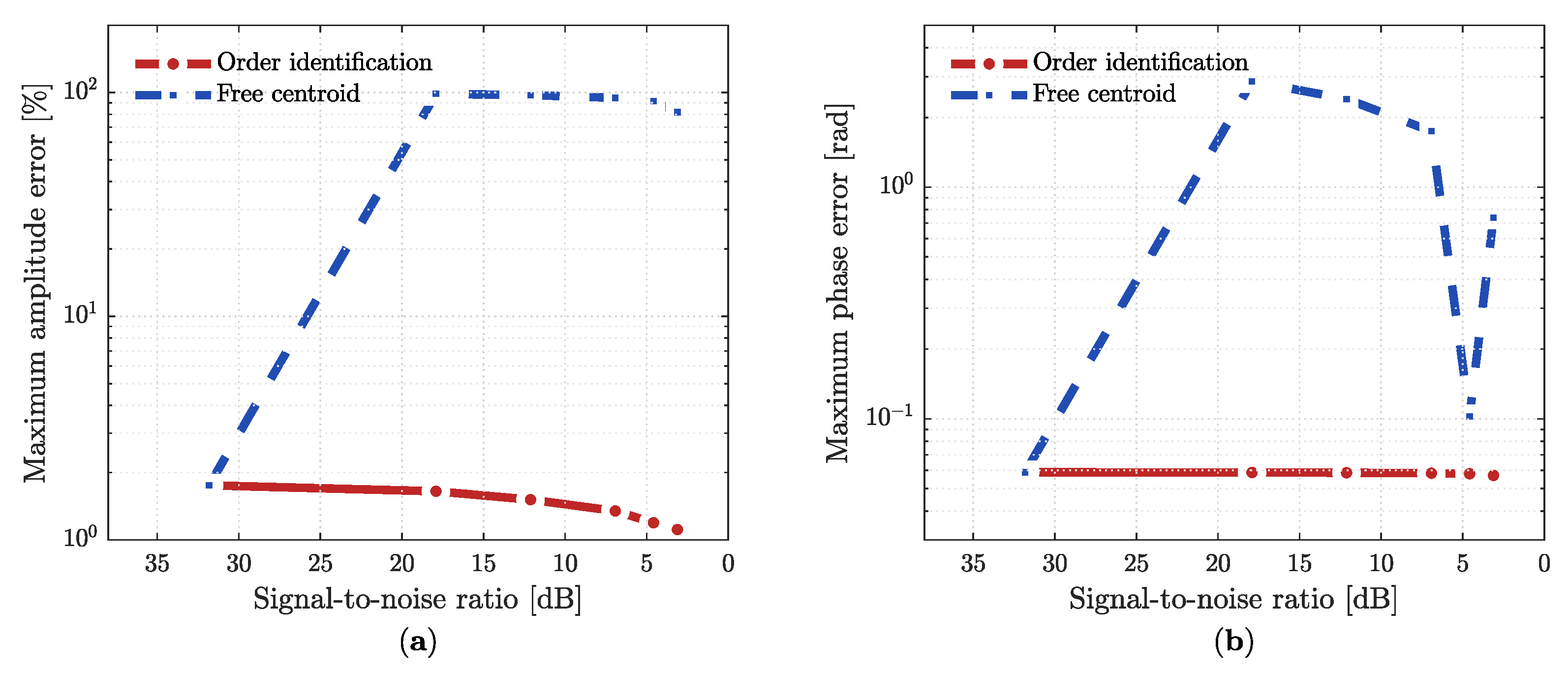
This section presents the numerical validation of the proposed integrated framework for velocity tracking control and hybrid multi-frequency vibration estimation in permanent magnet synchronous motor systems. Two representative case studies are considered in order to evaluate the robustness, adaptability, and estimation accuracy of the method under different electromechanical configurations and disturbance profiles. In addition to the two case studies, the estimation stage is assessed under an abrupt load-torque step, compared against benchmark estimators, evaluated in the presence of measurement noise across a range of signal-to-noise ratios.

In the first case study, a surface-mounted permanent magnet synchronous motor with equal direct and quadrature inductances ($L_d=L_q$) is analyzed under the influence of a multiple-frequency load-torque disturbance whose components are defined as speed orders of the rotor angular velocity, ${\mathrm{\Omega }}_{L,j}=h_j\omega$, in accordance with the model of Section 2. Because this machine operates along piecewise-constant speed plateaus, the resulting harmonic frequencies remain constant within each plateau and shift in steps between plateaus. In the second case study, a salient-pole interior permanent magnet synchronous motor configuration with different inductances ($L_d\ne L_q$) is considered, where the external disturbance torque follows a smooth Bézier trend driven by a continuously varying speed reference, so that its order-based harmonics sweep continuously in frequency; amplitude-modulated components are additionally included, and a maximum-torque-per-ampere strategy [40] is employed so that the machine operates with a nonzero direct-axis current and the magnetic saliency actively participates in the dynamics.

The desired rotor velocity trajectory ${\omega }^{\star }$ is selected as a smooth reference signal in order to evaluate the tracking performance of the proposed control scheme under disturbed operating conditions. To avoid abrupt transients and guarantee smooth acceleration and deceleration phases, the reference velocity is defined as a polynomial Bézier trajectory [41], expressed as

$${\omega }^{\star }=\left\{\begin{array}{cc}{\omega }_i,\hfill & 0\le t<T_1,\hfill \\ {\omega }_i+\left({\omega }_f-{\omega }_i\right){\mathcal{B}}_z\left(t,T_1,T_2\right),\hfill & T_1\le t\le T_2,\hfill \\ {\omega }_f,\hfill & t>T_2,\hfill \end{array}\right.$$

(29)

where ${\omega }_i$ and ${\omega }_f$ denote the initial and final rotor velocities of each segment, respectively, and $T_1$, $T_2$ are the corresponding initial and final transition times. Moreover, ${\mathcal{B}}_z\left(t,T_1,T_2\right)$ is a Bézier curve given by

$${\mathcal{B}}_z\left(t,T_1,T_2\right)={\displaystyle \sum _{k=0}^8}{c}_k{\left({\displaystyle \frac{t-T_1}{T_2-T_1}}\right)}^{k+8},$$

(30)

which is employed to achieve a smooth motion from some initial velocity ${\omega }_i$ to another ${\omega }_f$ within the time interval $[T_1,T_2]$.

The numerical simulations were performed using two representative parameter sets that capture the characteristic behavior of surface-mounted and interior permanent magnet synchronous motors. The isotropic machine corresponds to a representative surface-mounted permanent magnet synchronous motor, in which the direct- and quadrature-axis inductances are equal. The salient-pole machine corresponds to a representative interior permanent magnet traction motor configuration, in which $L_d\ne L_q$ owing to the interior permanent magnet structure. The parameters employed in the simulations are summarized in

Table 1. Electrical and mechanical parameters of the isotropic PMSM.

Parameter	Symbol	Value
Rated power	P	2 kW
Stator resistance	$R_s$	0.675 $\mathrm{\Omega }$
Direct inductance	$L_d$	6.5 mH
Quadrature inductance	$L_q$	6.5 mH
Pole pairs	$n_p$	3
Permanent magnet magnetic flux	${\lambda }_m$	0.29 Wb
Rotor inertia	J	0.0425 kg·m2
Viscous friction coefficient	b	0.02 N·m·s
Number of stator slots	$N_s$	36
PM remanence	$B_r$	1.2 T
Winding connection	-	Three-phase, Y
Winding layout	-	Distributed
PM material	-	NdFeB

and

Table 2. Electrical and mechanical parameters of the salient-pole PMSM.

Parameter	Symbol	Value
Rated power	P	20 kW
Stator resistance	$R_s$	0.02 $\mathrm{\Omega }$
Direct inductance	$L_d$	1.50 mH
Quadrature inductance	$L_q$	3.57 mH
Pole pairs	$n_p$	4
Permanent magnet magnetic flux	${\lambda }_m$	0.892 Wb
Rotor inertia	J	1 kg·m2
Viscous friction coefficient	b	$1.0\times {10}^{-4}$ N·m·s
Number of stator slots	$N_s$	48
PM remanence	$B_r$	1.2 T
Winding connection	-	Three-phase, Y
Winding layout	-	Distributed
PM material	-	NdFeB

.

The difference between $L_d$ and $L_q$ in the second configuration reflects the magnetic saliency characteristic of interior permanent magnet synchronous motors, which introduces a reluctance-torque term into the total electromagnetic torque equation, active only when a nonzero direct-axis current is injected [42]. For the magnet-dominated machine considered here, the reluctance contribution is modest at the operating currents; nevertheless, the maximum-torque-per-ampere strategy operates the machine with $i_d^{\star }\ne 0$, so that the magnetic saliency actively participates in the dynamics rather than remaining dormant as under the conventional $i_d^{\star }=0$ operation. Considering both configurations allows evaluating the robustness of the proposed control and vibration estimation framework under two distinct electromagnetic structures: isotropic and salient-pole machines. Demonstrating the method on both machines further shows that the control-based reconstruction and the harmonic estimation are independent of the specific electromagnetic structure and of the underlying torque-production mechanism. The rated powers listed in Table 1 and Table 2 are nameplate values; both case studies operate along low-to-moderate speed profiles, so the instantaneous mechanical power remains below the rated figure.

5.1. Estimation and Control of a Surface-Mounted PMSM Under Velocity-Dependent Multifrequency Disturbance

In the first case study, an isotropic surface-mounted permanent magnet synchronous motor with equal direct and quadrature inductances is considered. This configuration eliminates the reluctance torque contribution and reduces the nonlinear coupling between the electromagnetic and mechanical subsystems, providing a scenario in which the performance of the proposed framework can be evaluated without the additional complexity introduced by magnetic saliency.

The disturbance signal acting on the motor shaft is expressed as the superposition of a constant load torque and four oscillatory components, consistent with the model established in Section 2, as

$${\tau }_L={\tilde{\tau }}_L+{\displaystyle \sum _{j=1}^4}{\tau }_{L,j}cos\left({\theta }_{L,j}-{\phi }_{L,j}\right),{\displaystyle \frac{d}{dt}}{\theta }_{L,j}=h_j\omega ,$$

(31)

where ${\tilde{\tau }}_L=10\mathrm{N}·\mathrm{m}$ represents a constant static load torque acting on the rotor shaft, $h_j$ is the speed order of the j-th component, and ${\theta }_{L,j}$ is its instantaneous phase. The harmonic parameters proposed for the oscillatory components are presented in

Table 3. Amplitudes ${\tau }_{L,j}$, speed orders $h_j$, and phases ${\phi }_{L,j}$ of the velocity-dependent multifrequency disturbance considered for the surface-mounted PMSM.

j	${\mathit{\tau }}_{\mathit{L},\mathit{j}}$ [N·m]	${\mathit{h}}_{\mathit{j}}$ (Order)	${\mathit{\phi }}_{\mathit{L},\mathit{j}}$ [rad]
1	2.5	1	$\pi /4$
2	3.2	2	$\pi /6$
3	2.2	3	$\pi /8$
4	2.3	4	$\pi /9$

.

The constant component ${\tilde{\tau }}_L$ models a static mechanical resistance applied to the rotor, such as a fixed gravitational load or a sustained friction force, representing the simplest and most common form of load disturbance in practical synchronous motor applications. Unlike the Bézier profile employed in the second case study, this term introduces no temporal variation and therefore does not alter the spectral content of the disturbance signal, acting solely as a constant offset superimposed on the oscillatory components.

The four oscillatory components are defined as the first four speed orders of the rotor angular velocity, so that their instantaneous frequencies ${\mathrm{\Omega }}_{L,j}=h_j\omega$ scale with the operating speed, in agreement with the physical mechanisms that generate torque ripple and load disturbances in permanent magnet synchronous motor drives [43]. The selected orders span the principal rotordynamic harmonics, from the once-per-revolution component to higher-order mechanical harmonics.

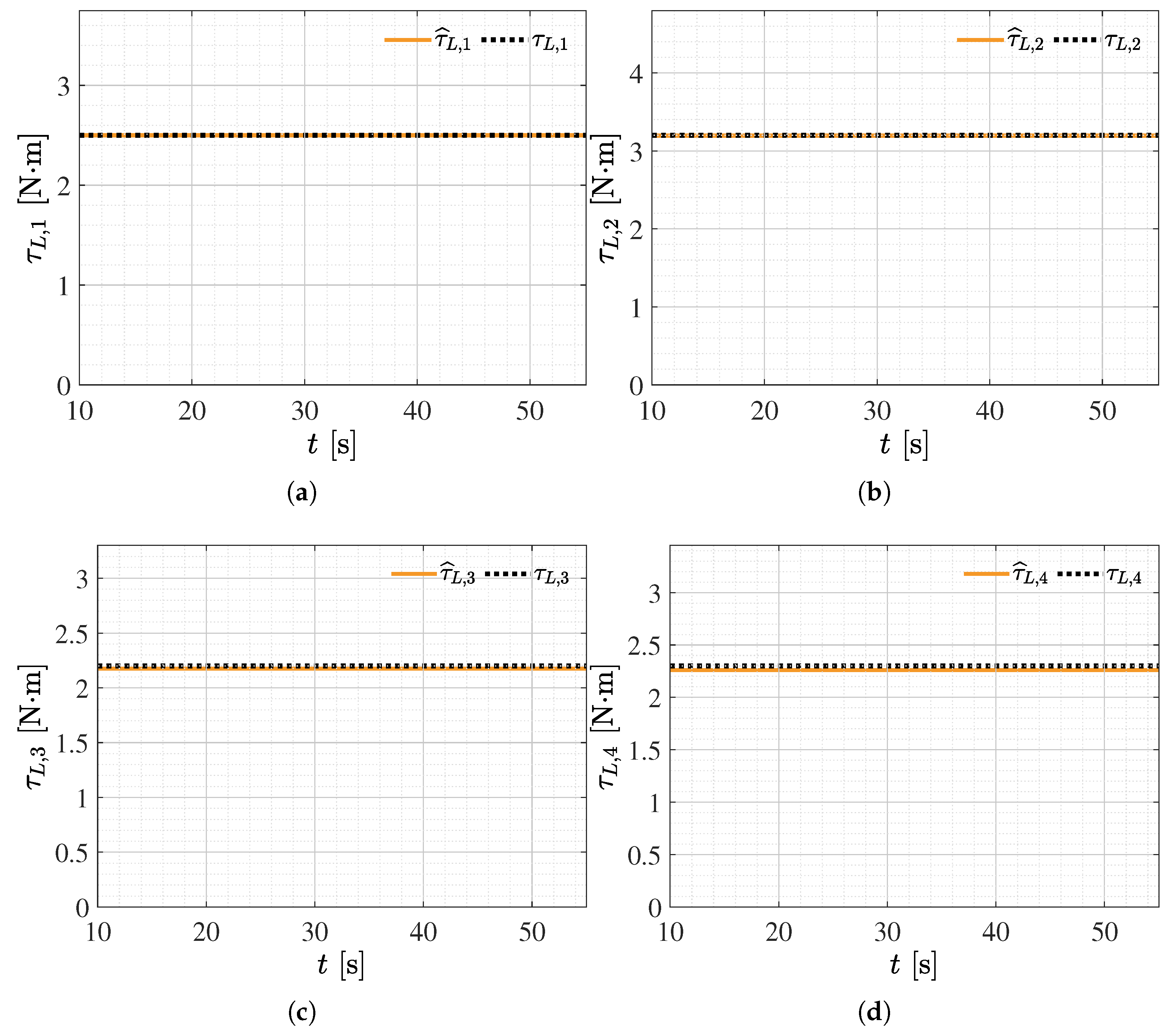
The first component ($h_1=1$, the once-per-revolution $1\times$ order) represents rotor mass unbalance and eccentricity, the most common source of velocity-synchronous vibration, with an amplitude of 2.5 N·m. The second component ($h_2=2$, $2\times$) corresponds to shaft misalignment and coupling asymmetries, with an amplitude of 3.2 N·m, representing the dominant contribution to the oscillatory disturbance energy. The third and fourth components ($h_3=3$ and $h_4=4$) capture higher-order mechanical harmonics associated with bearing and coupling imperfections, as well as torque ripple produced by the non-sinusoidal distribution of the stator windings and the discrete pole structure of the machine [44], with amplitudes of 2.2 and 2.3 N·m, consistent with reported torque-ripple magnitudes in surface-mounted machines operating under inverter-fed conditions, where ripple coefficients typically reach values up to 3.1% of the reference torque [45]. Because all four components are speed orders, their absolute frequencies cluster together at low-speed plateaus, spanning $[20,80]$ rad/s at $\omega =20$ rad/s, and spread apart at high speed, spanning $[80,320]$ rad/s at $\omega =80$ rad/s; this velocity-dependent clustering is precisely the condition that motivates the variational refinement stage of the proposed hybrid decomposition.

The velocity tracking performance of the proposed control scheme is evaluated under the order-based multifrequency disturbance defined in Equation (31). The reference trajectory ${\omega }^{\star }$ is a multi-segment profile constructed from Bézier polynomials. As detailed in

Table 4. Reference velocity profile segments demanded to the surface-mounted PMSM.

Interval [s]	Transition	${\mathit{\omega }}^{\mathbf{\star }}$ [rad/s]
$0\to 4$	Start-up	$0\to 60$
$4\to 10$	Regulation	60
$10\to 14$	Partial braking	$60\to 35$
$14\to 22$	Regulation	35
$22\to 26$	Strong acceleration	$35\to 80$
$26\to 34$	Regulation	80
$34\to 40$	Hard braking	$80\to 20$
$40\to 48$	Regulation	20
$48\to 52$	Return	$20\to 60$
$52\to 60$	Final regulation	60

, the profile spans ${\omega }^{\star }\in [0,80]$ rad/s across ten segments over $t\in [0,60]$ s, combining acceleration, braking, and regulation phases. This type of profile is representative of electric vehicle traction and variable-speed industrial drives.

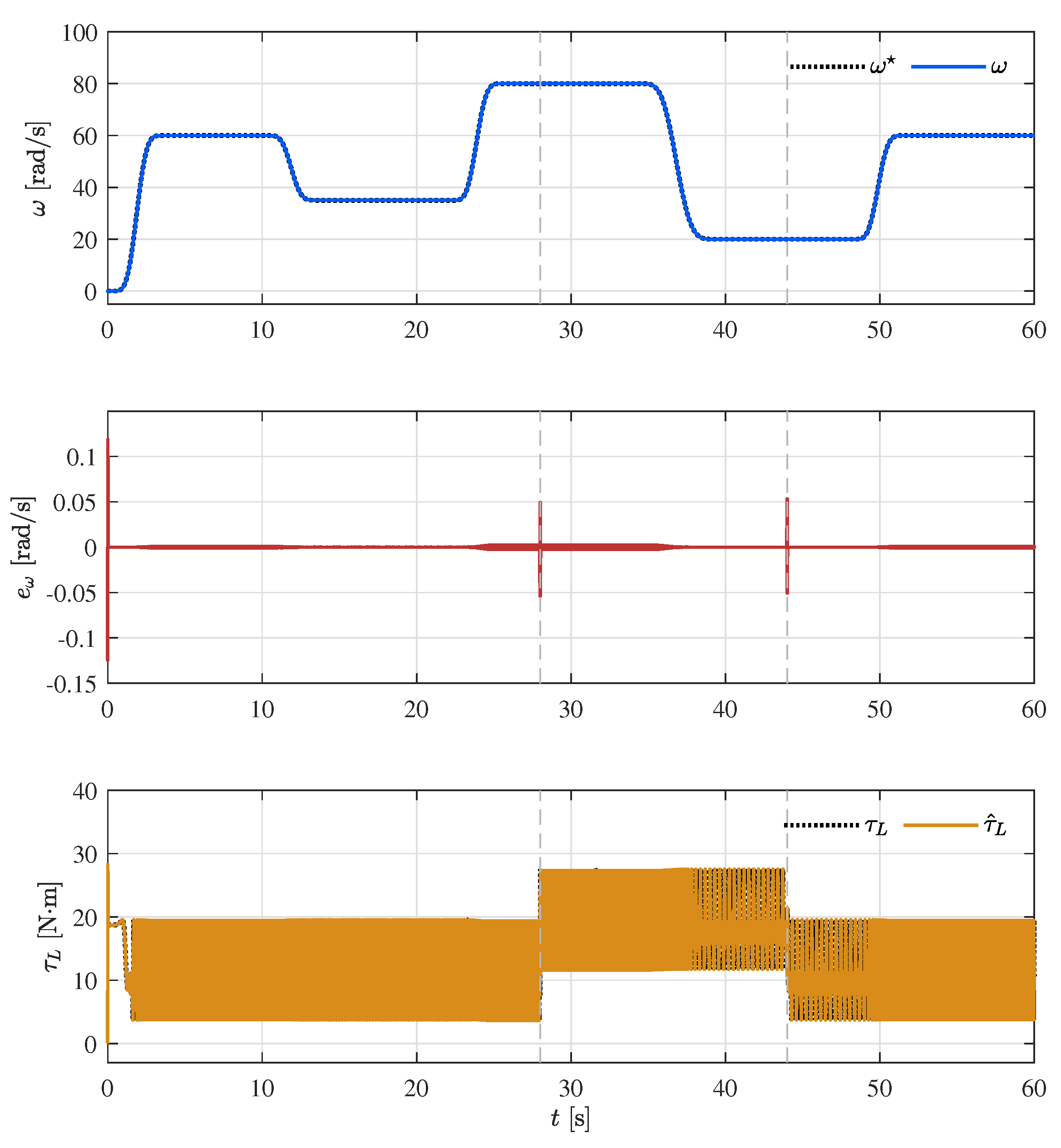
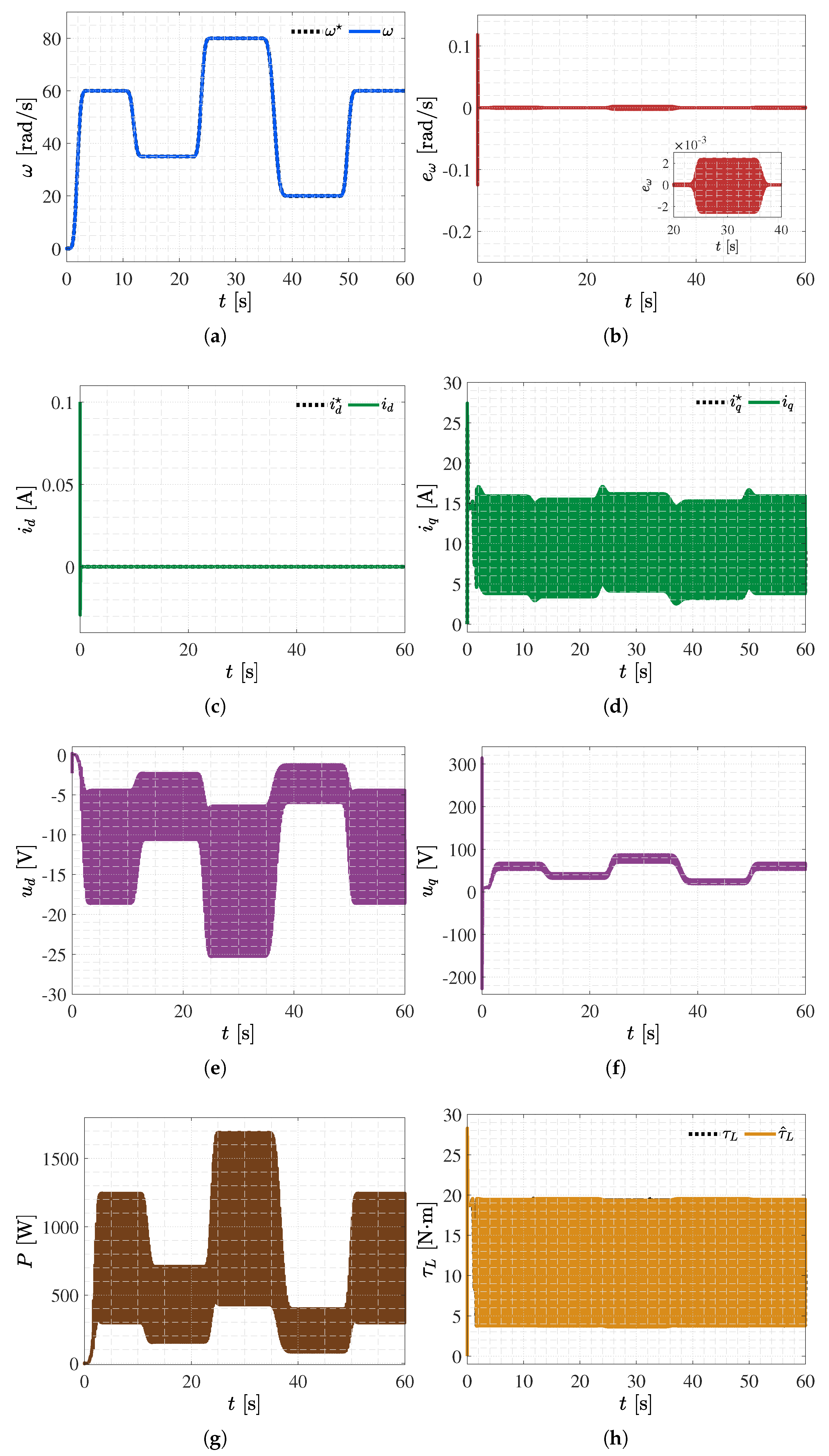
Figure 3 presents the closed-loop response of the surface-mounted permanent magnet synchronous motor system.

Figure 3a shows $\omega$ tracking ${\omega }^{\star }$ without overshoot at any transition. The tracking error in Figure 3b peaks at $|e_{\omega }|\approx 0.12$ rad/s during start-up and settles to an RMS value of $6.7\times {10}^{-4}$ rad/s, with steady peaks below $2.6\times {10}^{-3}$ rad/s; the residual oscillation reflects the order-based harmonic content of ${\tau }_L$, which the finite-bandwidth compensator rejects down to this level. The direct-axis current in Figure 3c converges at $i_d=0$ A, confirming effective axis decoupling under the $i_d^{\star }=0$ strategy. The quadrature current in Figure 3d tracks $i_q^{\star }$ accurately, peaking at ≈27 A during start-up and settling to $i_q\in [2.5,17.1]$ A; notably, the frequency of its ripple changes with the operating speed, becoming denser at the $\omega =80$ rad/s plateau and sparser at $\omega =20$ rad/s, which is the time-domain signature of the velocity-dependent disturbance. The direct-axis voltage in Figure 3e operates within $u_d\in [-25,0]$ V, dominated by the decoupling term. The quadrature voltage in Figure 3f scales with the velocity profile, with mean values of $u_q\approx 23$ V at $\omega =20$ rad/s, 36 V at 35 rad/s, 58 V at 60 rad/s, and 76 V at 80 rad/s, besides a brief start-up transient. 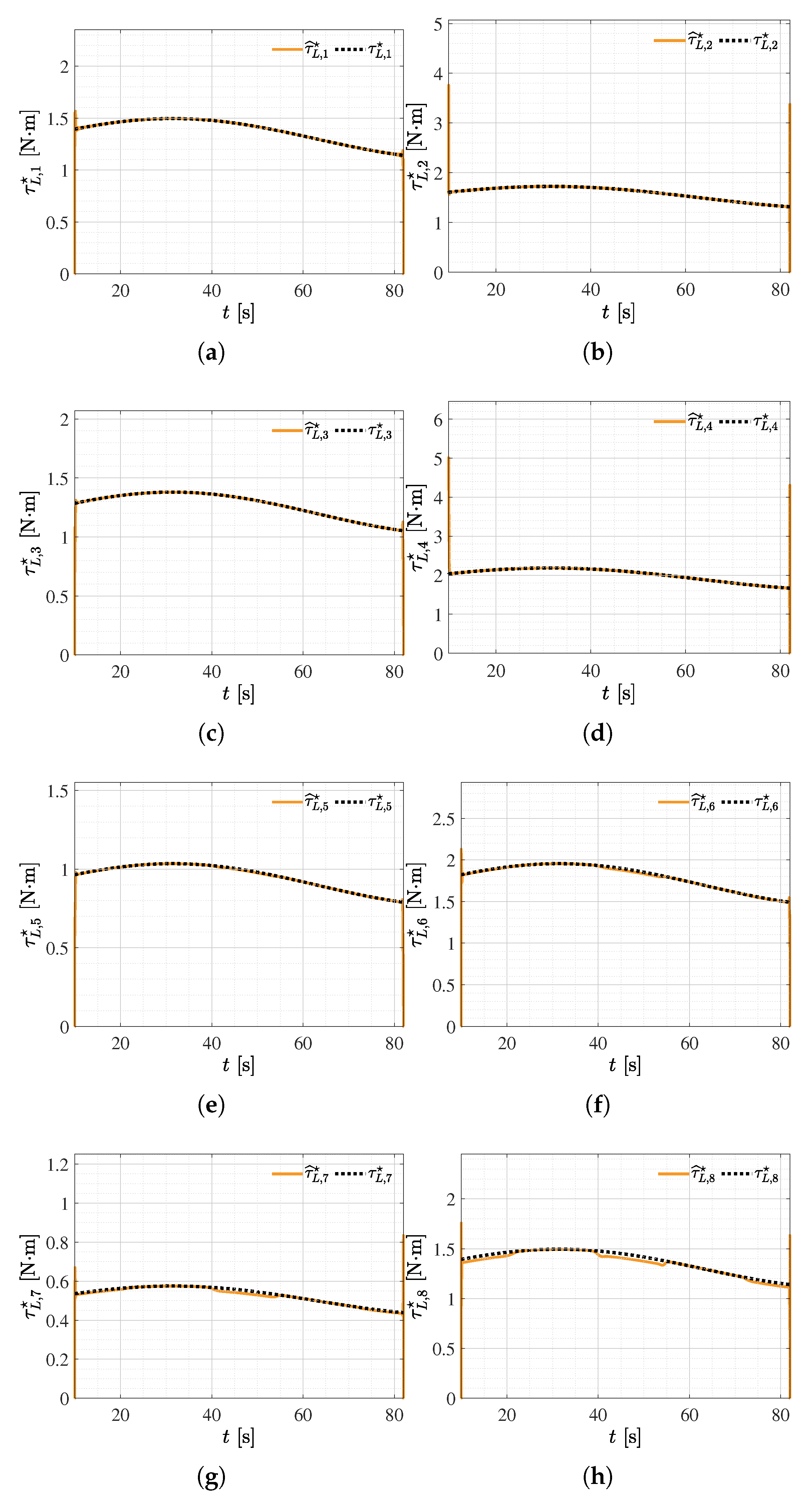The mechanical power in Figure 3g peaks at ≈1.7 kW at $\omega =80$ rad/s and drops to about 200 W on average (peaking near 400 W) at $\omega =20$ rad/s. The load torque estimate ${\widehat{\tau }}_L$ in Figure 3h tracks the disturbance ${\tau }_L\in [3.7,19.6]$ N·m with a steady-state reconstruction error of $0.11$ N·m RMS.

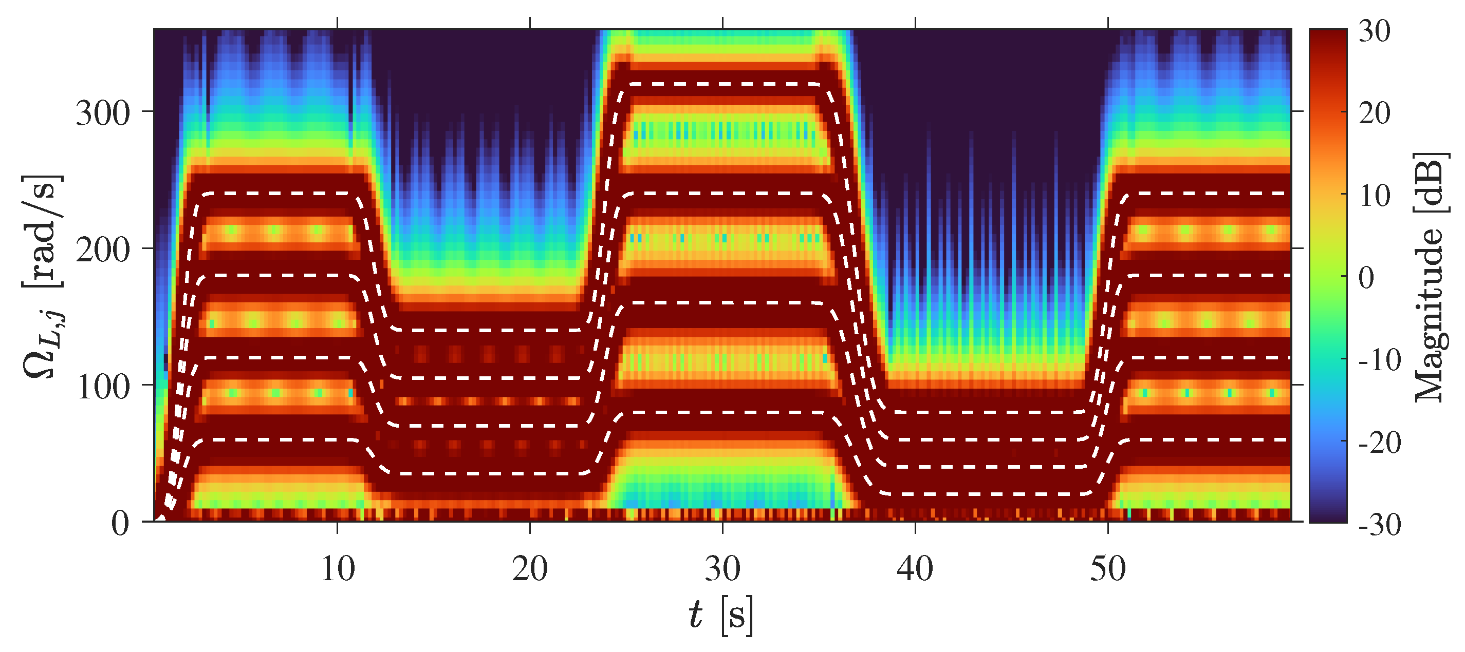
The velocity-dependent nature of the disturbance is made explicit in Figure 4, which shows the time–frequency map of the reconstructed disturbance ${\widehat{\tau }}_L$. The four harmonic ridges remain locked onto the order lines $h_j\omega$ throughout the profile, rising to approximately $[80,160,240,320]$ rad/s on the $\omega =80$ rad/s plateau and descending to $[20,40,60,80]$ rad/s on the $\omega =20$ rad/s plateau. A per-plateau spectral analysis confirms this quantitatively: the dominant peaks of ${\widehat{\tau }}_L$ fall within $0.6\%$ of the predicted orders $h_j\omega$ at every regulation level, a deviation set by the frequency resolution of the finite plateau window. This demonstrates that the proposed framework reconstructs harmonics whose frequencies vary with the operating speed, rather than the fixed-frequency components assumed in idealized stationary models.

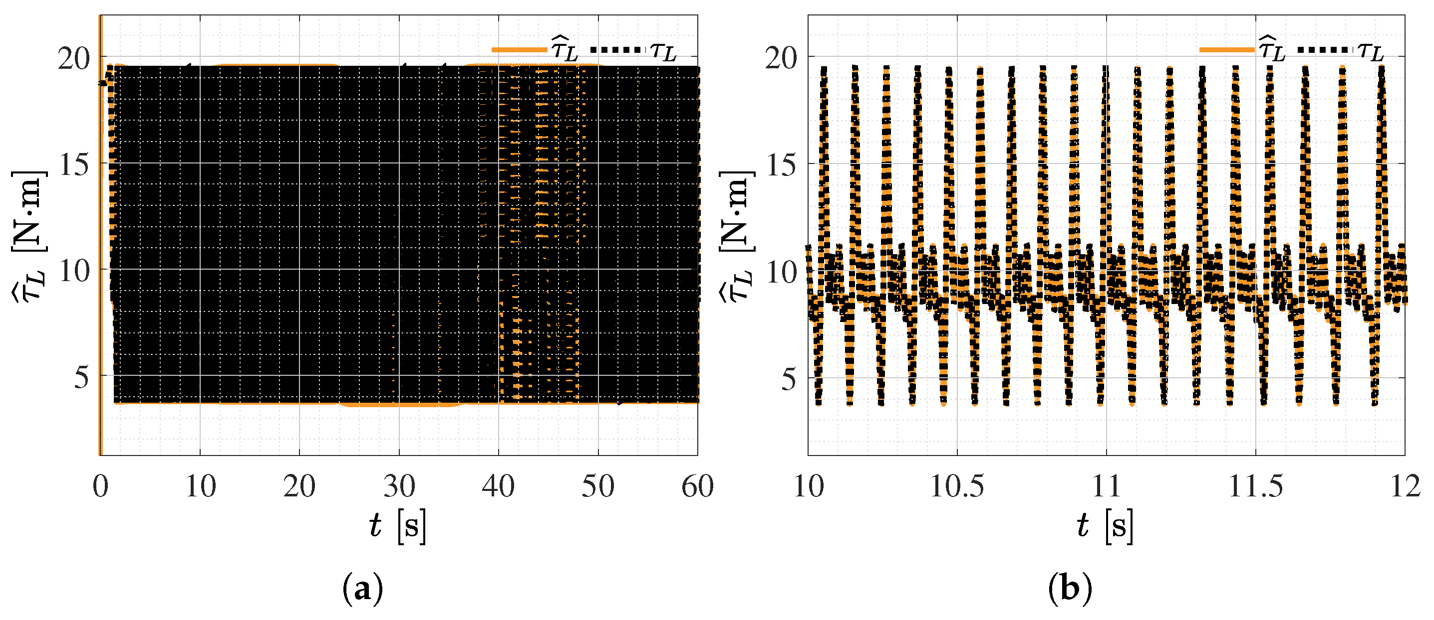
The disturbance torque estimation capability of the proposed framework is assessed by comparing the actual disturbance signal ${\tau }_L$, defined in Equation (31), with its estimate ${\widehat{\tau }}_L$ obtained from the internal control structure as established in Section 3. Figure 5 presents both signals over the complete simulation horizon.

The estimate reproduces both the constant offset and the order-based oscillatory structure across all four components. The agreement between ${\tau }_L$ and ${\widehat{\tau }}_L$ confirms that the proposed scheme simultaneously captures the static load contribution and the complete speed-dependent harmonic content of the disturbance without requiring additional measurement instrumentation. As expected from the finite observer bandwidth, the reconstruction error grows mildly with frequency, from about $4\times {10}^{-4}$ N·m at the $\omega =20$ rad/s plateau to $0.21$ N·m at $\omega =80$ rad/s, while remaining below $1.5\%$ of the peak-to-peak disturbance amplitude at all operating speeds.

The reconstructed disturbance ${\widehat{\tau }}_L$ delivered by the internal observer is processed by the hybrid Empirical–Variational mode decomposition to separate the individual oscillatory modes. Because the disturbance is order-based, the instantaneous frequency of each component, ${\mathrm{\Omega }}_{L,j}=h_j\omega$, varies with the operating speed, and a decomposition applied directly in the time domain would have to track non-stationary spectral peaks. To preserve the stationarity assumed by the variational stage, the decomposition is instead performed in the angular domain: ${\widehat{\tau }}_L$ is resampled at uniform increments of the rotor mechanical angle ${\theta }_m$, where each speed order appears as a component of constant order. The rotor angle is the same signal already used for the $dq$ transformation, so no additional instrumentation is required. In this domain the variational stage separates the modes blindly, recovering the four speed orders $h_j=\{1,2,3,4\}$ without any prior knowledge of their values, after which the modes are mapped back to the time domain and the Hilbert transform yields the amplitude, instantaneous frequency, and phase of each component.

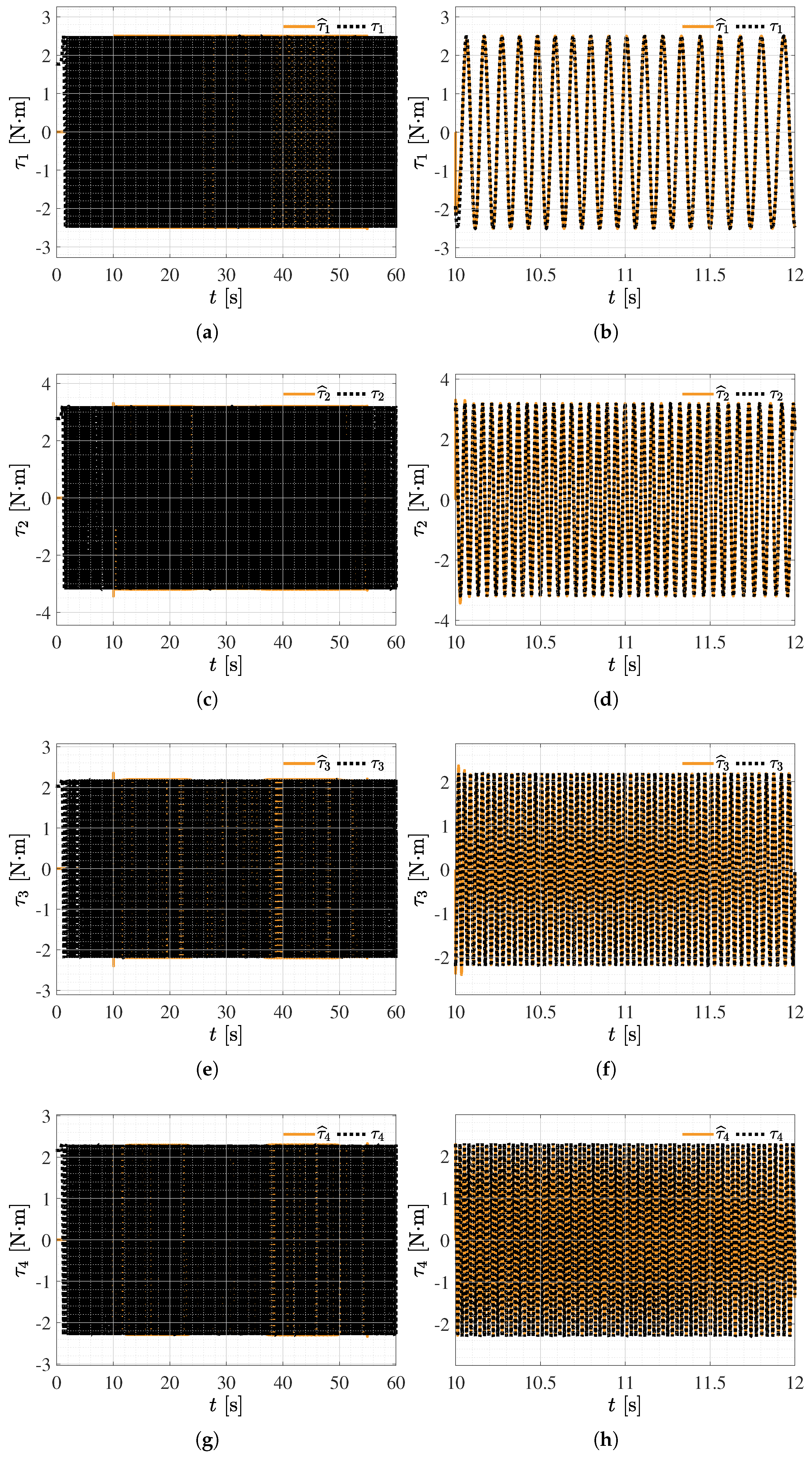
Figure 6 presents the four modes extracted by the hybrid decomposition, each shown as its complete response together with a corresponding zoomed view.

Each extracted mode corresponds to one speed order and reproduces the corresponding term ${\tau }_{L,j}cos({\theta }_{L,j}-{\phi }_{L,j})$ of the disturbance model in Equation (31), with ${\dot{\theta }}_{L,j}=h_j\omega$ and $j=1,2,3,4$. The amplitude and phase of each mode are constant while its frequency follows the speed; the Hilbert transform recovers all three quantities from the decomposed modes, as described below.

The estimated amplitudes ${\widehat{\tau }}_{L,j}$ are compared against the reference values ${\tau }_{L,j}$ defined in Equation (31). Figure 7 presents the amplitude of each mode over the analysis interval.

The estimated amplitudes closely track the reference values for all four components. The larger deviations are confined to the higher orders, whose absolute frequencies are the fastest and are therefore the most affected by the finite observer bandwidth, but the error remains below $1.8\%$ in every case.

Table 5. Amplitude estimation error metrics for the surface-mounted machine under the order-based multifrequency disturbance. The last column reports the Mean-Squared Error (MSE) of the estimated instantaneous amplitude envelope over the analysis window.

Component	${\mathit{\tau }}_{\mathit{L},\mathit{j}}$ [N·m]	${\widehat{\mathit{\tau }}}_{\mathit{L},\mathit{j}}$ [N·m]	Error [N·m]	Error [%]	MSE
1	2.5	2.500	$2.5\times {10}^{-4}$	0.010	$4.98\times {10}^{-4}$
2	3.2	3.195	$5.1\times {10}^{-3}$	0.160	$4.03\times {10}^{-4}$
3	2.2	2.176	$2.44\times {10}^{-2}$	1.110	$2.49\times {10}^{-3}$
4	2.3	2.259	$4.07\times {10}^{-2}$	1.770	$2.29\times {10}^{-3}$

confirms that the amplitude error stays below $1.8\%$ for every component, the largest corresponding to the highest-order mode ($h_4=4$), whose frequency reaches 320 rad/s at the top speed.

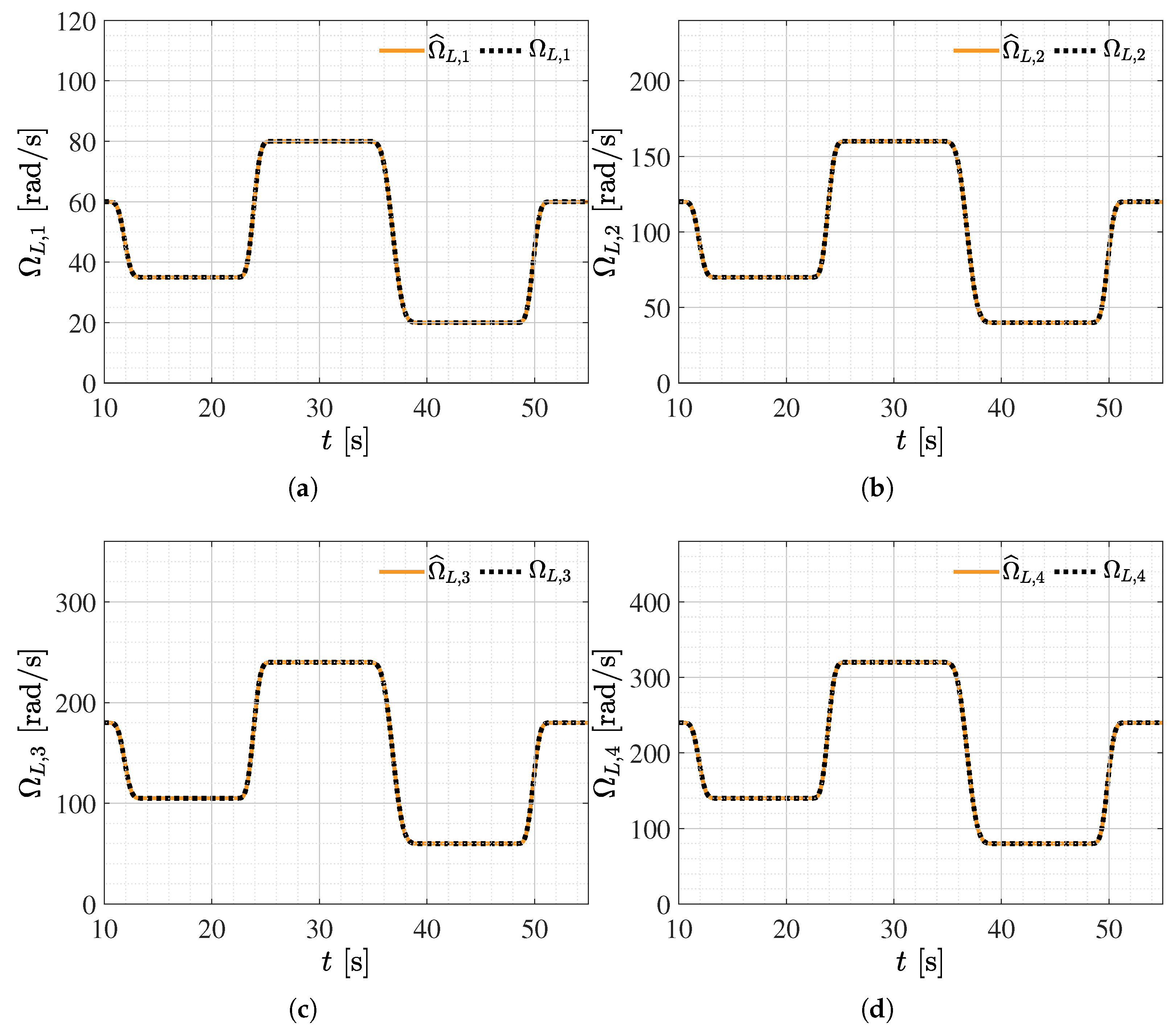
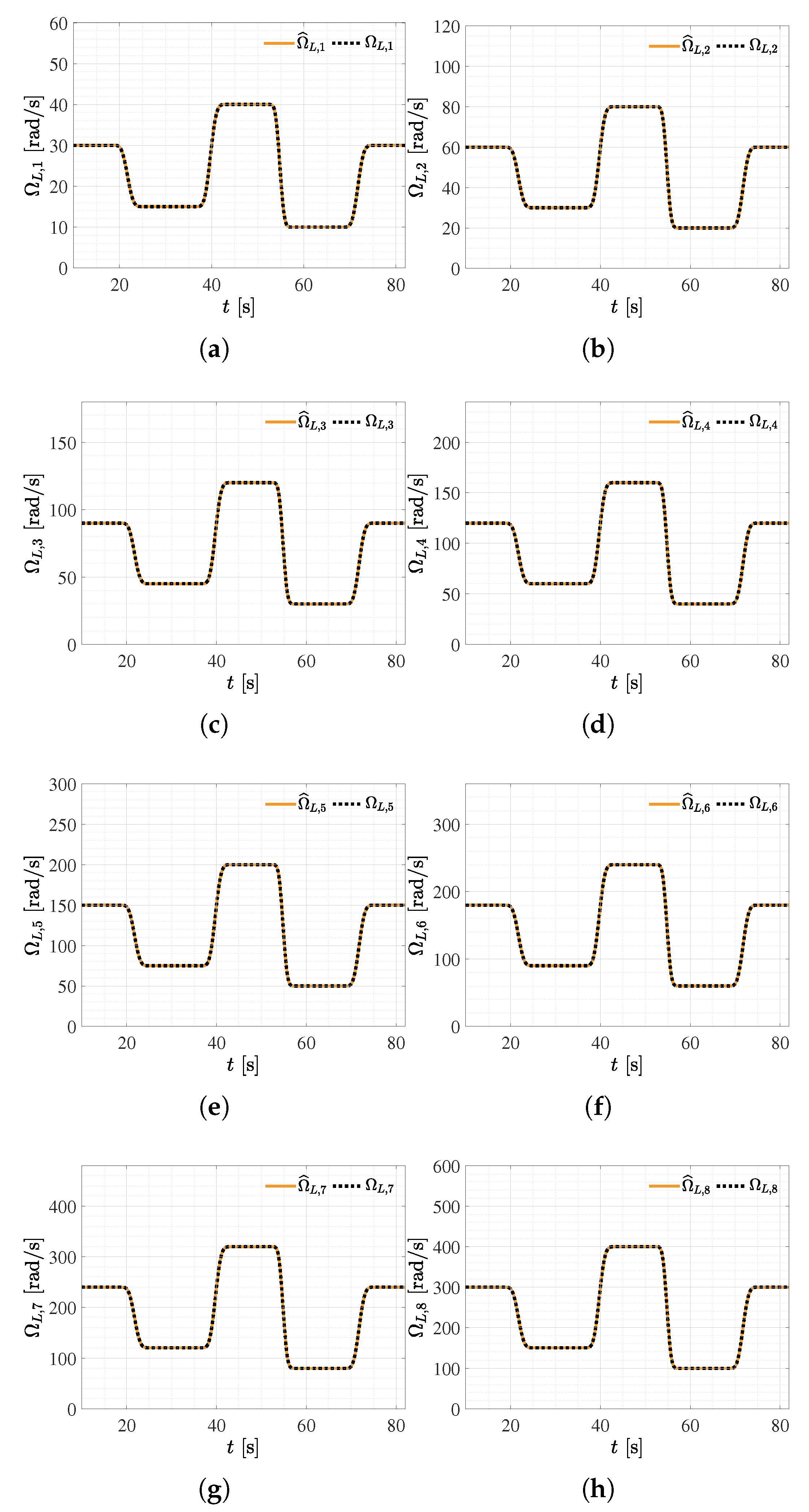
The instantaneous frequency of each mode follows the order line ${\mathrm{\Omega }}_{L,j}=h_j\omega$. Figure 8 presents the estimated instantaneous frequencies together with their order references, and the time–frequency map of Figure 4 shows the four ridges locked onto the order lines throughout the run.

Table 6. Speed orders identified by the hybrid decomposition for the surface-mounted machine under the order-based multifrequency disturbance, together with the frequency range spanned by each order over the velocity profile.

Component	Reference Order ${\mathit{h}}_{\mathit{j}}$	Identified Order ${\widehat{\mathit{h}}}_{\mathit{j}}$	${\mathbf{\Omega }}_{\mathit{L},\mathit{j}}$ Range [rad/s]
1	1	1.000	20–80
2	2	2.000	40–160
3	3	3.000	60–240
4	4	4.000	80–320

shows that the decomposition identifies the four speed orders exactly, so that the instantaneous frequency of every mode is reconstructed as ${\widehat{h}}_j\omega$ and sweeps with the operating speed, confirming that the spectral structure is preserved as the velocity changes.

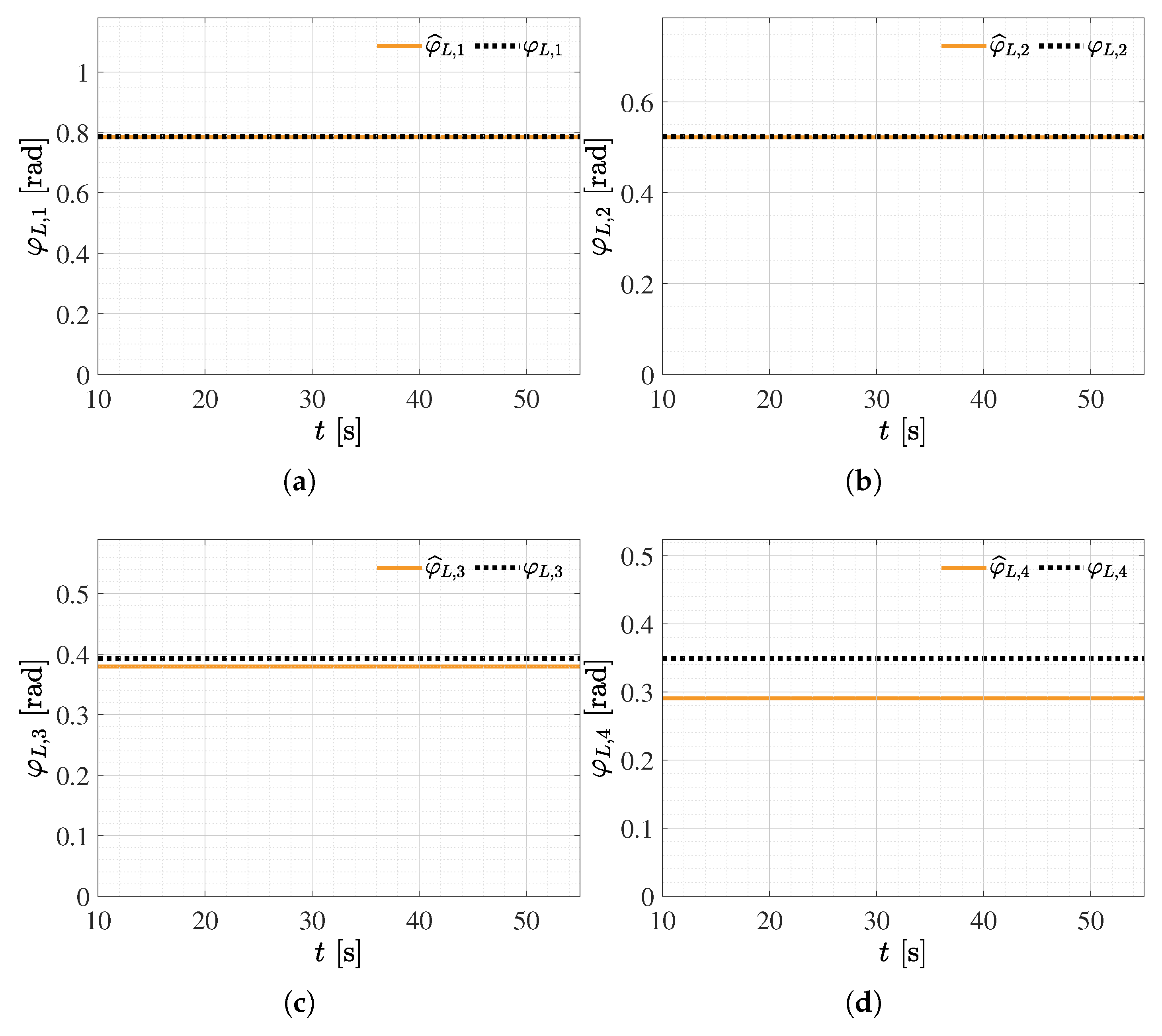
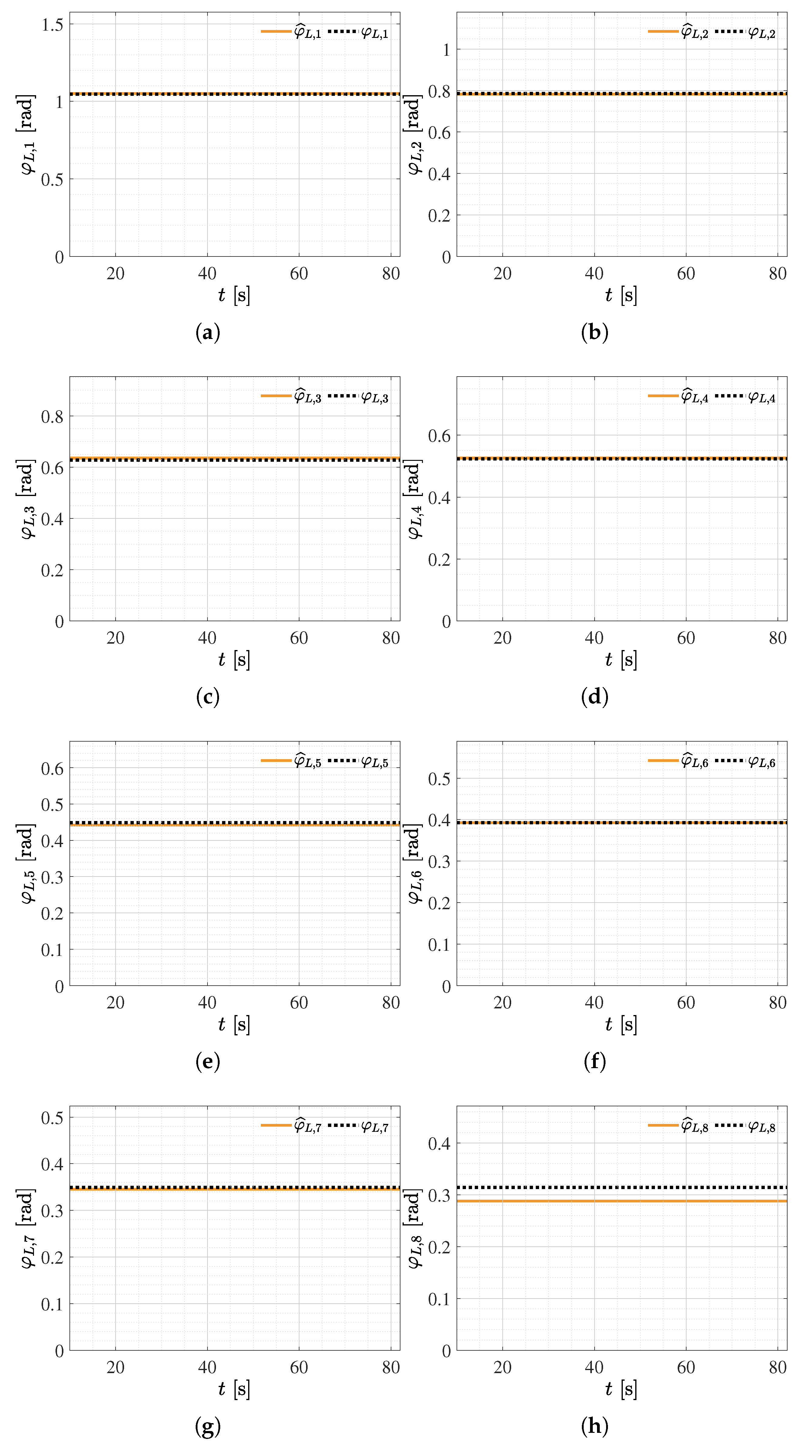
The instantaneous phases ${\widehat{\phi }}_{L,j}$ are obtained from the angle of the analytic signal associated with each extracted mode. Figure 9 presents the estimated phases together with their references.

Table 7. Phase estimation error metrics for the surface-mounted machine under the order-based multifrequency disturbance. The MSE column reports the mean-squared error of the estimated instantaneous phase over the analysis window.

Component	${\mathit{\phi }}_{\mathit{L},\mathit{j}}$ [rad]	${\widehat{\mathit{\phi }}}_{\mathit{L},\mathit{j}}$ [rad]	Error [rad]	Error [%]	MSE
1	0.7854	0.7852	$2.4\times {10}^{-4}$	0.031	$4.56\times {10}^{-5}$
2	0.5236	0.5221	$1.5\times {10}^{-3}$	0.286	$6.41\times {10}^{-5}$
3	0.3927	0.3795	$1.32\times {10}^{-2}$	3.362	$5.02\times {10}^{-4}$
4	0.3491	0.2903	$5.88\times {10}^{-2}$	16.84	$6.95\times {10}^{-3}$

confirms accurate phase recovery, with errors below $1.4\times {10}^{-2}$ rad for the first three components. The largest deviation appears in the fourth mode, whose faster oscillation and smaller relative energy make its phase the most sensitive to the residual reconstruction error; the absolute error nonetheless remains below $0.06$ rad.

To place these results in context, the hybrid decomposition is compared against three classical estimators applied to the same reconstructed signal ${\widehat{\tau }}_L$: a Short-Time Fourier Transform (STFT) evaluated over the quasi-stationary plateaus, a recursive Kalman filter that estimates the harmonic coefficients from the order phases ${\theta }_{L,j}=h_j{\theta }_m$ supplied by the measured rotor angle, and a single fixed-frequency Fourier fit that ignores the speed dependence. The extended Kalman filter is a recursive estimator. Because the order phases are taken from the measured angle rather than treated as unknown states, the amplitude estimation is linear, and the filter therefore reduces to a linear Kalman filter.

Table 8. Benchmark of disturbance-component estimators for the surface-mounted machine under the order-based multifrequency disturbance, reporting the amplitude error of each component and the total root-mean-square reconstruction error.

Method	Comp. 1 Error [%]	Comp. 2 Error [%]	Comp. 3 Error [%]	Comp. 4 Error [%]	Total RMSE [N·m]
Hybrid EMD–VMD	0.01	0.16	1.11	1.77	0.110
STFT	0.02	0.08	0.75	1.30	≈0.07
Kalman filter	0.00	0.15	1.06	2.83	0.064
Fixed-frequency FFT	98.2	95.6	95.6	95.9	3.65

reports the amplitude error of each harmonic component together with the Root Mean Square Error (RMSE) of the reconstructed load torque signal.

The comparison shows that every estimator that respects the speed dependence of the harmonics, namely the hybrid EMD–VMD, the per-plateau short-time Fourier transform, and the recursive Kalman filter, recovers all four amplitudes with errors below $2.9\%$ and total reconstruction errors in the range $0.06$–$0.11$ N·m, whereas the fixed-frequency Fourier fit collapses, with amplitude errors above $95\%$ and a total error roughly two orders of magnitude larger, because demodulating a swept-frequency component at a single fixed frequency averages its energy to nearly zero. This confirms that the speed-dependent nature of the disturbance must be taken into account. The Kalman filter attains the lowest reconstruction error, but it presupposes that the harmonic order phases are supplied as a known regressor, and the per-plateau short-time Fourier transform likewise requires a prior segmentation of the record into quasi-stationary intervals; by contrast, the proposed hybrid decomposition operates blindly in the angular domain, matching their accuracy while additionally identifying the speed orders itself, from the rotor angle already available in the drive and without any externally supplied frequency information.

5.2. Estimation and Control of a Salient-Pole PMSM Under an Order-Based Bézier Disturbance Profile

In the second case study, the complexity of the electromechanical system is deliberately increased along two independent axes in order to assess the robustness of the proposed framework under demanding and realistic operating conditions. First, magnetic saliency is introduced by selecting $L_d\ne L_q$, which produces a nonlinear cross-coupling between the d- and q-axis dynamics, and is exploited through a maximum-torque-per-ampere strategy in which the direct-axis current reference is not fixed to zero. Second, and most importantly, the disturbance torque is no longer a stationary signal with a fixed constant offset, but is instead composed of a smooth Bézier polynomial trend superimposed with eight amplitude-modulated harmonic components whose energy content evolves continuously over time, producing a nonstationary disturbance profile of significantly greater complexity.

It should be noted that, for the magnet-dominated machine considered here, the reluctance torque contributes only marginally to the total electromagnetic torque. The purpose of this second case is therefore not to exploit a large reluctance torque, but to evaluate the framework under three genuinely distinct conditions with respect to the first case: the salient cross-coupled electrical dynamics, operation with a nonzero direct-axis current, and a substantially larger power and inertia scale. These differences make the salient case a non-trivial validation scenario.

Under the maximum-torque-per-ampere strategy, the direct-axis current reference is computed from the provisional quadrature reference $i_q^0$ produced by the velocity-tracking law of Section 3 so as to minimize the stator current magnitude required to deliver a given torque. Thus, the direct-axis reference follows the maximum-torque-per-ampere relation [40]

$$i_d^{\star }={\displaystyle \frac{{\lambda }_m-\sqrt{{\lambda }_m^2+8{(L_q-L_d)}^2{\left(i_q^0\right)}^2}}{4(L_q-L_d)}},$$

(32)

which is strictly negative for the salient-pole machine and reduces to the conventional $i_d^{\star }=0$ operation in the isotropic limit $L_d\to L_q$. The quadrature reference is then refined so that the demanded torque is delivered once the reluctance contribution is included:

$$i_q^{\star }={\displaystyle \frac{{\tau }_{\mathrm{des}}}{\frac{3}{2}{n}_p\left[{\lambda }_m+(L_d-L_q)i_d^{\star }\right]}},{\tau }_{\mathrm{des}}=\frac{3}{2}{n}_p{\lambda }_m{i}_q^0,$$

(33)

so that the reference pair of $i_d^{\star }$ and $i_q^{\star }$ jointly exploits the magnetic saliency while tracking the torque demanded by the velocity controller.

The motivation for adopting a Bézier polynomial as the baseline load profile is rooted in the physical behavior of real drive systems, particularly electric vehicles, where the load torque acting on the motor shaft is not constant but changes progressively as a function of operating conditions. During vehicle acceleration, uphill driving, or the progressive engagement of mechanical loads, the resistive torque increases gradually and smoothly rather than abruptly, depicting a profile that is well approximated by smooth polynomial trajectories. The Bézier polynomial efficiently captures this behavior, since it guarantees continuity of the load profile and its derivatives, avoiding discontinuities that would be physically unrealistic in mechanical systems with inertia. This makes the Bézier-based disturbance profile a representative and physically motivated scenario, and constitutes a closer approximation to the actual load conditions encountered in electric traction, industrial servo drives, and robotic actuation systems.

The baseline disturbance trend is described by a fifth-order Bézier polynomial defined as

$${\tilde{\tau }}_L=\left\{\begin{array}{cc}{y}_i,\hfill & t<t_i\hfill \\ y_i+(10u^3-15u^4+6u^5)(y_f-y_i),\hfill & t_i\le t\le t_f\hfill \\ y_f,\hfill & t>t_f\hfill \end{array}\right.$$

(34)

where

$$u={\displaystyle \frac{t-t_i}{t_f-t_i}},$$

(35)

and the parameters used in the simulation are $t_i=0\mathrm{s}$, $t_f=10\mathrm{s}$, $y_i=0$, and $y_f=6\mathrm{N}·\mathrm{m}$. This profile represents a gradual increase in load torque, modeling realistic operating conditions such as the progressive mechanical resistance experienced by an electric vehicle during an acceleration phase or an uphill driving maneuver.

The complete disturbance signal acting on the motor shaft is expressed as the superposition of the Bézier trend and eight amplitude-modulated oscillatory components, consistent with the model established in Section 2, as

$${\tau }_L={\tilde{\tau }}_L+\xi {\displaystyle \sum _{j=1}^8}{\tau }_{L,j}^{\star }cos\left({\theta }_{L,j}-{\phi }_{L,j}\right),{\displaystyle \frac{d}{dt}}{\theta }_{L,j}=h_j\omega ,$$

(36)

where the time-varying amplitude of each harmonic component is defined as

$${\tau }_{L,j}^{\star }={\tau }_{L,j}\left(1+\delta sin\left({\omega }_{m}t\right)\right),$$

(37)

and $\xi$ is a unit step activation function given by

$$\xi =\left\{\begin{array}{cc}0,\hfill & t<t_0\hfill \\ 1,\hfill & t\ge t_0\hfill \end{array}\right.$$

(38)

with $t_0=6\mathrm{s}$, $\delta =0.15$, and ${\omega }_m=0.05\mathrm{rad}/\mathrm{s}$. Here $h_j$ is the speed order of the j-th component and ${\theta }_{L,j}$ its instantaneous phase, so that the frequency of each harmonic, ${\mathrm{\Omega }}_{L,j}=h_j\omega$, scales with the rotor speed. The activation function $\xi$ models the sudden onset of oscillatory disturbances at $t_0$, representing the engagement of a mechanical load or the initiation of an operating regime in which harmonic excitations become significant, as occurs for instance when an electric vehicle transitions from a standstill to an active traction phase. The modulation term $\left(1+\delta sin\left({\omega }_{m}t\right)\right)$ introduces a slow sinusoidal variation in the amplitude of each harmonic component, capturing the nonstationarity of disturbance signals whose intensity fluctuates over time due to changes in operating velocity, load conditions, or thermal effects. The harmonic parameters are presented in

Table 9. Amplitudes ${\tau }_{L,j}$, speed orders $h_j$, and phases ${\phi }_{L,j}$ of the disturbance profile considered for the salient-pole PMSM.

j	${\mathit{\tau }}_{\mathit{L},\mathit{j}}$ [N·m]	${\mathit{h}}_{\mathit{j}}$ (Order)	${\mathit{\phi }}_{\mathit{L},\mathit{j}}$ [rad]
1	1.3	1	$\pi /3$
2	1.5	2	$\pi /4$
3	1.2	3	$\pi /5$
4	1.9	4	$\pi /6$
5	0.9	5	$\pi /7$
6	1.7	6	$\pi /8$
7	0.5	8	$\pi /9$
8	1.3	10	$\pi /10$

.

The eight components are defined as speed orders of the rotor angular velocity, spanning a wide range of orders ($h=1$ to $h=10$) so that the disturbance contains both closely spaced low-order harmonics and well-separated higher-order ones. This combination is a demanding test for the variational refinement stage, since closely spaced modes are the most difficult to separate.

The low-order components ($h=1$ to $h=4$) represent slow mechanical disturbances such as rotor unbalance, shaft misalignment, gear-meshing effects, and gradual variations in the external load. Their relatively large amplitudes reflect the sustained energy associated with these mechanical interactions over long time intervals. The intermediate orders ($h=5$, $h=6$) correspond to structural resonances and torsional oscillations emerging from the coupling between the motor shaft, the load transmission, and the bearing support structure [43]. The two highest orders ($h=8$, $h=10$) capture faster electromechanical harmonics produced by the non-sinusoidal distribution of the stator windings and the discrete pole structure of the machine [44], with amplitudes consistent with reported torque-ripple magnitudes in interior permanent magnet machines operating under inverter-fed conditions, where ripple coefficients typically reach values up to 3.1% of the reference torque [45]. Because all components are speed orders, the entire spectrum compresses toward low frequencies at the slow plateaus ($\omega =10$ rad/s) and expands at the faster ones ($\omega =40$ rad/s), so the decomposition stage must resolve the harmonics over a continuously shifting frequency support.

The overall structure of the disturbance signal, combining a smooth nonstationary Bézier trend, a step-activated onset of oscillatory components, and a slow amplitude modulation across all harmonics, reflects the expected behavior of load disturbances in real PMSM drive systems and constitutes a substantially challenging validation benchmark. This multifrequency nonstationary disturbance profile therefore provides a comprehensive and physically motivated test scenario for evaluating the robustness of the proposed control and estimation framework against the complex disturbance spectra encountered in practice.

The velocity tracking performance of the proposed control scheme is evaluated under the order-based nonstationary multifrequency disturbance defined in Equation (36). The reference trajectory ${\omega }^{\star }$ is a multi-segment profile constructed from Bézier polynomials. As detailed in

Table 10. Reference velocity profile segments demanded to the salient-pole PMSM.

Interval [s]	Transition	${\mathit{\omega }}^{\mathbf{\star }}$ [rad/s]
$0\to 8$	Start-up	$0\to 30$
$8\to 18$	Regulation	30
$18\to 26$	Partial braking	$30\to 15$
$26\to 36$	Regulation	15
$36\to 44$	Strong acceleration	$15\to 40$
$44\to 52$	Regulation	40
$52\to 58$	Hard braking	$40\to 10$
$58\to 68$	Regulation	10
$68\to 76$	Return	$10\to 30$
$76\to 84$	Final regulation	30

, the profile spans ${\omega }^{\star }\in [0,40]$ rad/s across ten segments over $t\in [0,84]$ s, combining acceleration, braking, and regulation phases. This type of profile is representative of low-speed salient-pole PMSM drives in industrial positioning and heavy-load applications.

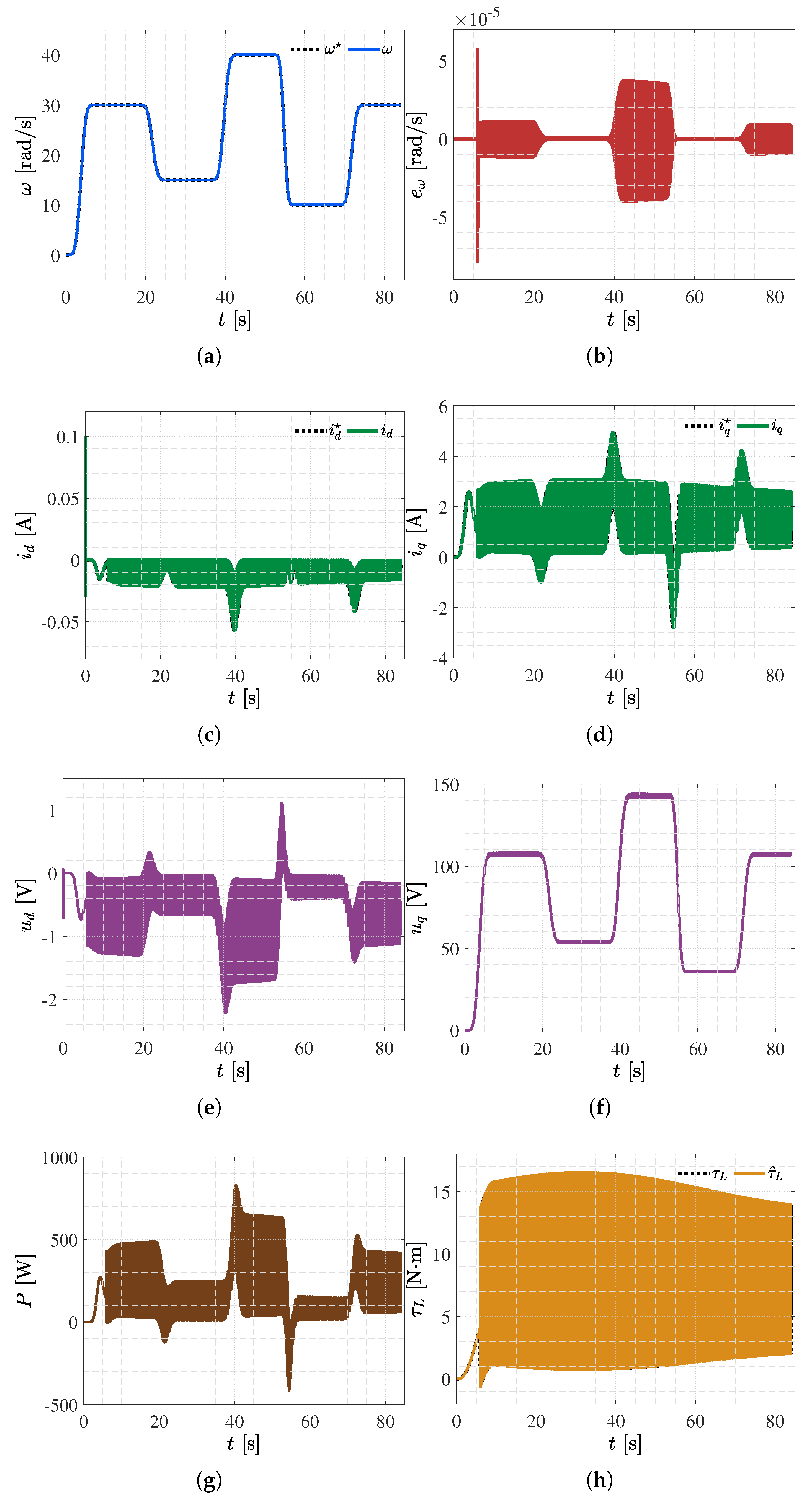
Figure 10 presents the closed-loop response of the synchronous motor system.

Figure 10a shows $\omega$ tracking ${\omega }^{\star }$ without overshoot at any transition. The tracking error in Figure 10b remains at the order of ${10}^{-5}$ rad/s throughout, with a brief peak of $\left|e_{\omega }\right| \approx 7.9 \times {10}^{-5}$ rad/s at the disturbance onset ($t_0=6$ s) and a steady RMS value of $9.4\times {10}^{-6}$ rad/s; its envelope widens at the $\omega =40$ rad/s plateau, where the order-based harmonics reach their highest frequencies. The direct-axis current in Figure 10c tracks the reference $i_d^{\star }<0$, operating within $i_d\in [-0.057,0]$ A; the magnitude is small because the machine is magnet-dominated, but the nonzero negative $i_d$ confirms that the framework operates correctly under the salient maximum-torque-per-ampere strategy rather than under the $i_d^{\star }=0$ condition. The quadrature current in Figure 10d tracks $i_q^{\star }$ accurately, with a start-up peak of ≈2.9 A and a steady range of $i_q\in [-2.8,5.0]$ A; its ripple frequency follows the operating speed, the time-domain signature of the order-based disturbance. The direct-axis voltage shown in Figure 10e operates within $u_d\in [-2.2,1.1]$ V. The quadrature voltage in Figure 10f scales with the velocity profile, with mean values of $u_q\approx 36$ V at $\omega =10$ rad/s, 54 V at 15 rad/s, 107 V at 30 rad/s, and 143 V at 40 rad/s. The mechanical power in Figure 10g peaks at ≈830 W during the strong acceleration to $\omega =40$ rad/s and exhibits regenerative-braking intervals reaching ≈$-420$ W during the hard braking phases. The load torque estimate ${\widehat{\tau }}_L$ in Figure 10h tracks the nonstationary disturbance ${\tau }_L\in [-0.6,16.5]$ N·m with a steady-state reconstruction error of $0.045$ N·m RMS, despite the Bézier trend, the step activation, and the amplitude modulation.

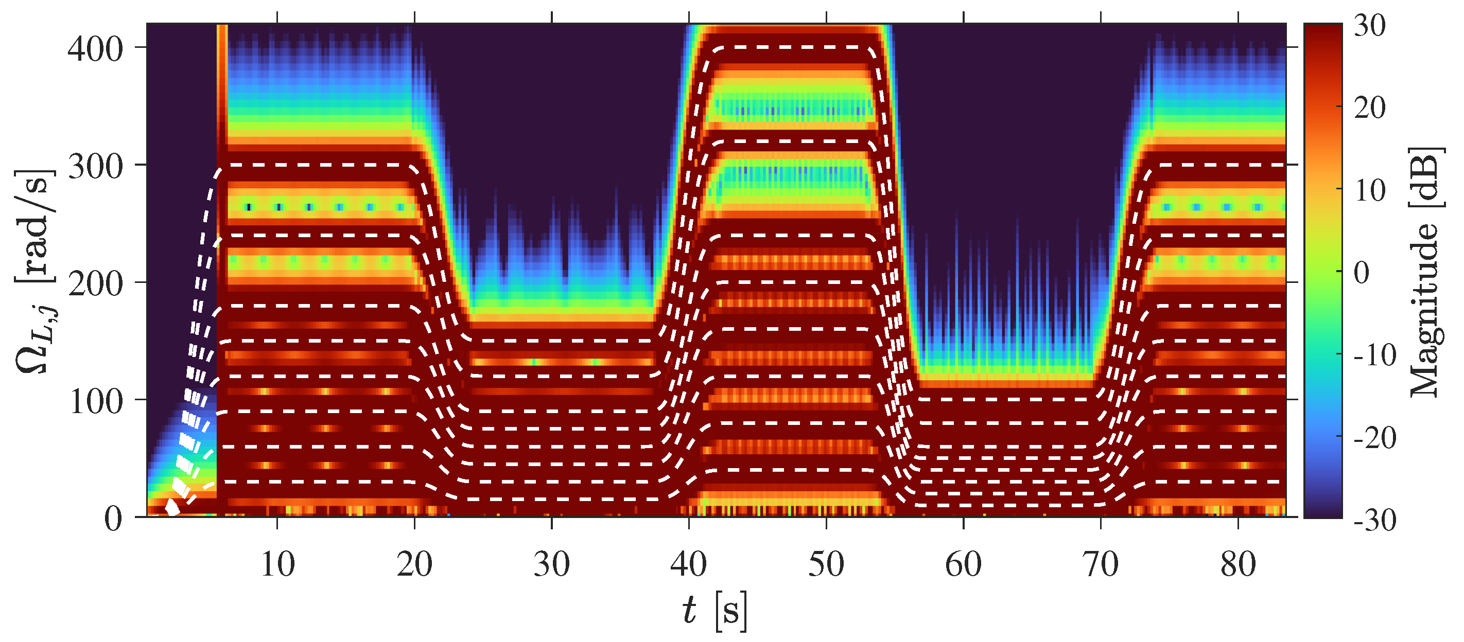
The order-based nature of the disturbance is made explicit in Figure 11, which shows the time–frequency map of the reconstructed disturbance ${\widehat{\tau }}_L$. The eight harmonic ridges appear at the activation instant $t_0=6$ s and remain locked onto the order lines $h_j\omega$ throughout the profile, expanding up to $[40,\dots ,400]$ rad/s on the $\omega =40$ rad/s plateau and compressing toward $[10,\dots ,100]$ rad/s on the $\omega =10$ rad/s plateau. A per-plateau spectral analysis confirms this quantitatively: the dominant peaks of ${\widehat{\tau }}_L$ coincide with the predicted orders $h_j\omega$ at every regulation level, recovering all eight components including the highest orders.

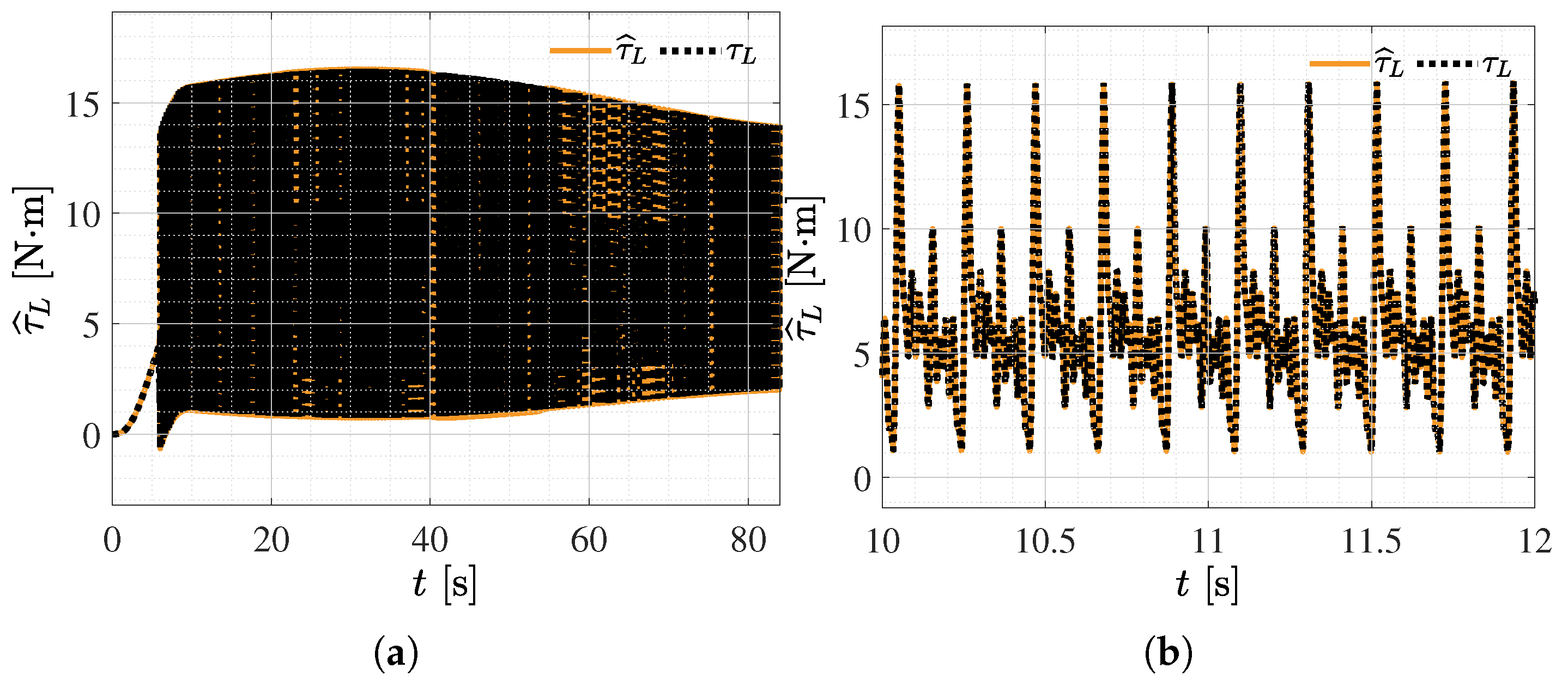
The disturbance torque estimation capability of the proposed framework is assessed by comparing the actual disturbance signal ${\tau }_L$, defined in Equation (36), with its estimate ${\widehat{\tau }}_L$ obtained from the internal control structure as established in Section 3. Figure 12 presents both signals over the complete simulation horizon.

The estimate reproduces both the nonstationary trend introduced by the Bézier profile and the superimposed order-based oscillatory components. The agreement between ${\tau }_L$ and ${\widehat{\tau }}_L$ confirms that the virtual sensor embedded in the control structure captures simultaneously the slow-varying load dynamics and the speed-dependent harmonic content of the disturbance, without requiring additional measurement instrumentation. As in the first case study, the reconstruction error grows with frequency, from about $2\times {10}^{-4}$ N·m at the $\omega =10$ rad/s plateau to $0.10$ N·m at $\omega =40$ rad/s, while remaining below $1\%$ of the peak-to-peak disturbance amplitude at all operating speeds.

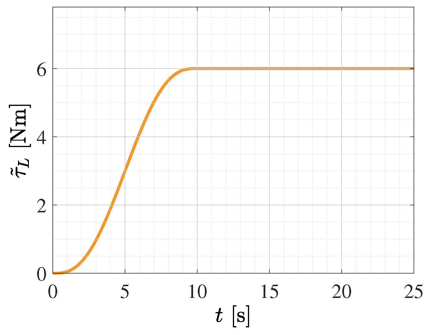
The isolated Bézier component ${\tilde{\tau }}_L$ is presented separately in Figure 13 to highlight its contribution to the overall disturbance energy.

This component represents the nonstationary behavior of the load, modeling a gradual increase in mechanical demand. The smooth evolution defines the global energy trend of the disturbance signal and constitutes the dominant low-frequency contribution to ${\tau }_L$.

The reconstructed disturbance ${\widehat{\tau }}_L$ is processed by the same hybrid Empirical–Variational decomposition introduced for the first case study, again performed in the angular domain so that every speed order appears as a stationary component. The second scenario is, however, considerably more demanding: the disturbance now contains eight harmonic components whose amplitudes are slowly modulated and whose orders span a wide and non-contiguous range ($h=\{1,2,3,4,5,6,8,10\}$, with the orders 7 and 9 absent), and whose absolute energies differ by almost a factor of four. Under these conditions a free-running variational decomposition is prone to merge the weakest components and to leave the gaps unpopulated. To make the separation reliable, the decomposition is preceded by a blind order-identification step: the angular spectrum of ${\widehat{\tau }}_L$ is computed and its dominant integer-order peaks are retained, which recovers exactly the set $\{1,2,3,4,5,6,8,10\}$ without any prior knowledge of the orders present. The variational stage then extracts each identified order, and the Hilbert transform yields the amplitude, instantaneous frequency, and phase of every component.

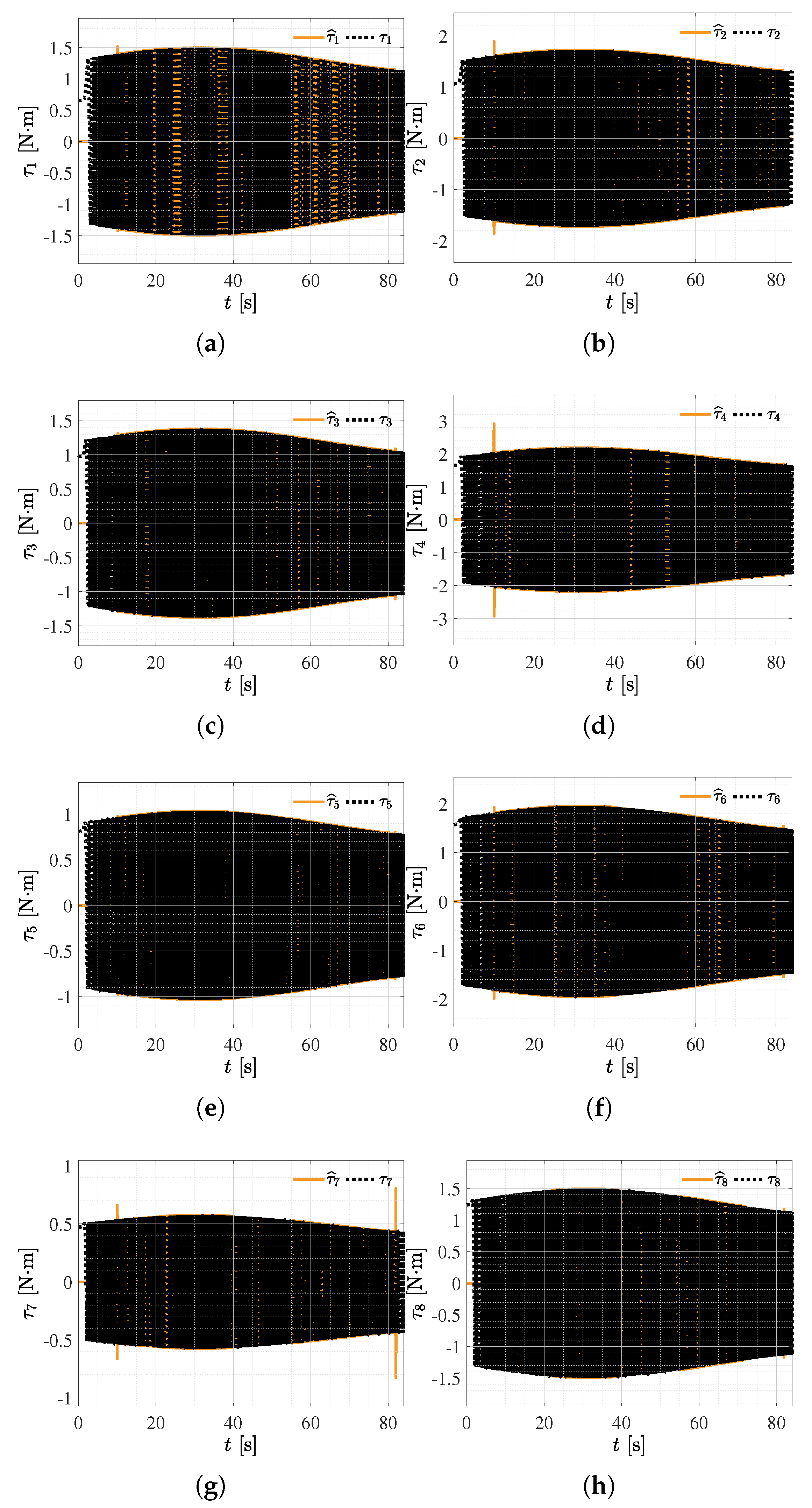
Figure 14 presents the eight modes extracted by the hybrid decomposition.

Each mode corresponds to one speed order and is described by the order-referenced harmonic ${\tau }_{L,j}={\tau }_{L,j}^{\star }cos({\theta }_{L,j}-{\phi }_{L,j})$, with ${\dot{\theta }}_{L,j}=h_j\omega$ and the slowly modulated amplitude ${\tau }_{L,j}^{\star }={\tau }_{L,j}(1+\delta sin{\omega }_{m}t)$ defined in Equation (37). Unlike the first case study, the amplitude of every mode is therefore time-varying, and the Hilbert envelope is expected to track this slow modulation rather than a constant value.

Figure 15 shows the estimated envelope of each mode together with its modulated reference ${\tau }_{L,j}^{\star }$. The envelopes follow the slow $\pm 15\%$ amplitude modulation imposed on the disturbance, confirming that the method captures the nonstationary amplitude content and not merely a mean level.

Table 11. Amplitude estimation error metrics for the salient-pole machine under the order-based nonstationary multifrequency disturbance. The nominal amplitudes are recovered after compensating for the slow modulation, and the MSE column reports the mean-squared error of the estimated instantaneous amplitude envelope over the analysis window.

Component	${\mathit{\tau }}_{\mathit{L},\mathit{j}}$ [N·m]	${\widehat{\mathit{\tau }}}_{\mathit{L},\mathit{j}}$ [N·m]	Error [N·m]	Error [%]	MSE
1	1.3	1.300	$2.2\times {10}^{-6}$	0.00	$2.04\times {10}^{-4}$
2	1.5	1.500	$4.3\times {10}^{-5}$	0.00	$6.94\times {10}^{-4}$
3	1.2	1.200	$1.1\times {10}^{-4}$	0.01	$9.14\times {10}^{-4}$
4	1.9	1.899	$6.7\times {10}^{-4}$	0.04	$1.62\times {10}^{-3}$
5	0.9	0.899	$1.0\times {10}^{-3}$	0.11	$7.60\times {10}^{-4}$
6	1.7	1.695	$5.0\times {10}^{-3}$	0.29	$3.77\times {10}^{-4}$
7	0.5	0.494	$5.6\times {10}^{-3}$	1.11	$2.11\times {10}^{-4}$
8	1.3	1.267	$3.3\times {10}^{-2}$	2.50	$1.19\times {10}^{-3}$

reports the recovered nominal amplitudes ${\tau }_{L,j}$, obtained after compensating for the known slow modulation, together with their error metrics. The estimates remain accurate for all eight components, with errors of at most $2.5\%$. As in the first case study, the error grows with the order of the component: the low orders are recovered almost exactly, whereas the highest order ($h=10$), whose absolute frequency reaches 400 rad/s, shows the largest deviation ($2.5\%$), reflecting the finite bandwidth of the disturbance observer at high frequencies.

The instantaneous frequency of each mode follows its order line ${\mathrm{\Omega }}_{L,j}=h_j\omega$ and therefore sweeps over a wide range as the speed varies between 10 and 40 rad/s. Figure 16 presents the estimated instantaneous frequencies together with their order references, and the time–frequency map of Figure 11 shows the eight ridges tracking the order lines along the nonstationary velocity profile.

Table 12. Speed orders identified by the hybrid decomposition for the salient-pole machine under the order-based nonstationary multifrequency disturbance, together with the frequency range spanned by each order over the velocity profile.

Component	Reference Order ${\mathit{h}}_{\mathit{j}}$	Identified Order ${\widehat{\mathit{h}}}_{\mathit{j}}$	${\mathbf{\Omega }}_{\mathit{L},\mathit{j}}$ Range [rad/s]
1	1	1.000	10–40
2	2	2.000	20–80
3	3	3.000	30–120
4	4	4.000	40–160
5	5	5.000	50–200
6	6	6.000	60–240
7	8	8.000	80–320
8	10	10.000	100–400

confirms that the decomposition identifies all eight speed orders exactly, including the non-contiguous high orders $h=8$ and $h=10$, so that the complete order structure is recovered despite the absence of orders 7 and 9.

The instantaneous phases ${\widehat{\phi }}_{L,j}$ are obtained from the analytic signal of each mode. Figure 17 presents the estimated phases together with their references, and

Table 13. Phase estimation error metrics for the salient-pole machine under the order-based nonstationary multifrequency disturbance. The MSE column reports the mean-squared error of the estimated instantaneous phase over the analysis window.

Component	${\mathit{\phi }}_{\mathit{L},\mathit{j}}$ [rad]	${\widehat{\mathit{\phi }}}_{\mathit{L},\mathit{j}}$ [rad]	Error [rad]	Error [%]	MSE
1	1.0472	1.0502	$-3.0\times {10}^{-3}$	−0.29	$3.15\times {10}^{-4}$
2	0.7854	0.7822	$3.2\times {10}^{-3}$	0.41	$3.07\times {10}^{-4}$
3	0.6283	0.6355	$-7.2\times {10}^{-3}$	−1.15	$1.29\times {10}^{-3}$
4	0.5236	0.5258	$-2.2\times {10}^{-3}$	−0.42	$5.40\times {10}^{-4}$
5	0.4488	0.4420	$6.8\times {10}^{-3}$	1.52	$1.41\times {10}^{-3}$
6	0.3927	0.3925	$2.0\times {10}^{-4}$	0.05	$4.82\times {10}^{-4}$
7	0.3491	0.3455	$3.6\times {10}^{-3}$	1.03	$6.21\times {10}^{-4}$
8	0.3142	0.2880	$2.62\times {10}^{-2}$	8.34	$2.51\times {10}^{-3}$

reports the error metrics.

Phase recovery is accurate for all components, with absolute errors of at most $7.2\times {10}^{-3}$ rad for the first seven modes. The largest deviation again appears in the highest-order mode ($h=10$), whose fast oscillation makes its phase the most sensitive to the residual reconstruction error; the absolute error nonetheless stays below $0.027$ rad.

The benchmark of

Table 14. Benchmark of disturbance-component estimators for the salient-pole machine under the order-based nonstationary multifrequency disturbance, reporting the mean and maximum amplitude error and the total root-mean-square reconstruction error.

Method	Mean Amp. Error [%]	Max. Amp. Error [%]	Total RMSE [N·m]
Hybrid EMD–VMD	0.5	2.5	0.047
STFT	10.0	12.1	>1
Kalman filter	11.1	12.8	0.52
Fixed-frequency FFT	98.3	99.7	2.88

compares the proposed decomposition against the same classical estimators used in the first case study. The contrast is now sharper than in the stationary-plateau scenario, for two compounding reasons. First, the Bézier-driven velocity profile varies continuously and offers no extended constant-speed intervals, so the per-plateau short-time Fourier transform can only be evaluated over short quasi-stationary windows and its mean amplitude error rises to about $10\%$, while the fixed-frequency Fourier fit fails almost completely, with a mean error above $98\%$. Second, and more importantly, the amplitude of every harmonic is slowly modulated: the recursive Kalman filter, which assumes constant harmonic coefficients, cannot follow this modulation, and its mean amplitude error grows to about $11\%$, in contrast to the first case study where it matched the proposed method. The proposed angular-domain decomposition, by contrast, tracks the amplitude through the Hilbert envelope and, after compensating the known modulation, keeps the mean amplitude error near $0.5\%$ and below $2.5\%$ for every component, reconstructing the full disturbance with an RMS error of $0.047$ N·m. This demonstrates that the envelope-based angular-domain formulation is essential when both the operating speed and the disturbance amplitudes vary continuously, a regime in which windowed time-domain methods and constant-amplitude recursive filters degrade.

Together with the first case study, these results show that the proposed framework recovers the amplitude, frequency, and phase of every speed order across two machines of very different scale and under both stationary-plateau and continuously varying operating conditions, while consistently outperforming classical spectral estimators on speed-dependent disturbances.

5.3. Robustness to Measurement and Actuator Noise

To assess the robustness of the proposed estimation framework, the surface-mounted machine is operated under signal-proportional noise injected into the control voltages. The noise model follows the structure proposed for algebraic identification under noisy conditions [46]: each control voltage is contaminated by a bounded random signal proportional to its own magnitude,

$$u_{\{d,q\}}^{\mathrm{noisy}}=u_{\{d,q\}}+{\zeta }_{\{d,q\}}\left|u_{\{d,q\}}\right|,{\zeta }_{\{d,q\}}={\epsilon }_u\left[{\varrho }_{\{d,q\}}-0.5+sgn\left({\nu }_{\{d,q\}}\right)\right],$$

(39)

where ${\varrho }_{\{d,q\}}$ are uniformly distributed random variables on $[0,1]$, ${\nu }_{\{d,q\}}$ are independent zero-mean unit-variance white-noise signals, and ${\epsilon }_u$ sets the noise level. The contaminated voltages are applied to the machine within the closed loop, so that the perturbation propagates through the current, velocity, and observer dynamics and reaches the reconstructed disturbance ${\widehat{\tau }}_L$; the hybrid decomposition therefore operates on a contaminated signal.

The noise level ${\epsilon }_u$ is swept and, for each value, the voltage signal-to-noise ratio, measured jointly over both control voltages $u_d$ and $u_q$ across the analysis window, is computed while the four order components are estimated. This study compares the two variants of the proposed angular-domain decomposition already used in the case studies. In the free-centroid variant, employed as the main method in the first case study, the mode centres are updated from the data during the variational optimization, so that the decomposition itself searches for the dominant frequencies. In the order-identification variant, introduced in the second case study, the dominant integer orders are first detected in the angular spectrum and the mode centres are then locked to them and kept fixed. This order-identification stage is precisely what prevents the variational filters from drifting towards broadband noise. Figure 18 and

Table 15. Estimation error of the four order components versus voltage signal-to-noise ratio, for the two variants of the proposed decomposition. The three central columns report the order-identification variant (maximum amplitude error, maximum phase error, and reconstruction RMSE); the last column reports the maximum amplitude error of the free-centroid variant, which collapses once the signal-to-noise ratio falls below about 30 dB.

${\mathit{\epsilon }}_{\mathit{u}}$	Signal-to-Noise Ratio [dB]	Max. Amp. Error [%]	Max. Phase Error [rad]	Recon. RMSE [N·m]	Free-Centroid Amp. Error [%]
0	∞ (clean)	1.77	0.059	0.110	1.77
0.01	31.8	1.75	0.059	0.110	1.75
0.05	17.9	1.65	0.059	0.112	98.70
0.10	12.1	1.51	0.059	0.117	97.43
0.20	6.9	1.35	0.058	0.137	94.75
0.30	4.6	1.19	0.058	0.171	91.77
0.50	3.1	1.11	0.057	0.319	81.78

report the resulting estimation errors as a function of the signal-to-noise ratio for the two variants.

For the order-identification variant, the amplitude and phase estimates are essentially insensitive to the injected noise: the maximum amplitude error remains between $1.1\%$ and $1.8\%$ and the maximum phase error below $0.06$ rad across the entire swept range, from the clean case down to a signal-to-noise ratio of about 3 dB, and the four integer orders are correctly recovered at every level. Only the reconstruction RMSE grows monotonically with the noise, from $0.11$ N·m in the clean case to $0.32$ N·m at the lowest signal-to-noise ratio, as expected from the broadband residual that the variational filters do not remove; the order amplitudes and phases nonetheless remain accurate throughout, because the mode centres are held at the identified integer orders and therefore do not track the noise. The largest level considered, ${\epsilon }_u=0.5$ with a signal-to-noise ratio of ≈3 dB, lies close to the stability boundary of the closed loop, beyond which the observer states begin to diverge, which delimits the meaningful range of the study.

The comparison in Figure 18 isolates the role of the order-identification stage. Both variants coincide at high signal-to-noise ratio, recovering the four orders with the same $1.8\%$ amplitude and $0.06$ rad phase accuracy as the noise-free case study, but the free-centroid variant, whose mode centres are updated from the data, loses the order structure as soon as the signal-to-noise ratio falls below about 30 dB: it still recovers the orders at 32 dB yet collapses by 18 dB, with amplitude errors near $99\%$, because its centres are captured by the high-frequency noise. The order-identification variant, by locking the centres to the integer orders detected in the angular spectrum, sustains an accurate characterization roughly 15 dB further down, to about 3 dB. These results confirm that the spectral order-identification stage is the key element providing noise robustness, and that the proposed framework retains an accurate harmonic characterization under realistic levels of measurement and actuator noise.

5.4. Response to External Load-Torque Steps

To evaluate the closed-loop behaviour under the abrupt load changes that occur in practice, two external load-torque steps are superimposed on the order-based disturbance of the first case study. A step of $+8$ N·m is applied at $t=28$ s, while the machine operates on the $\omega =80$ rad/s regulation plateau, and a step of $-8$ N·m is applied at $t=44$ s, on the $\omega =20$ rad/s plateau, so that the static component of the load torque follows the sequence $10\to 18\to 10$ N·m. The oscillatory order-based components remain active throughout, so the steps are added on top of the speed-dependent harmonic disturbance rather than replacing it.

Figure 19 shows the closed-loop response. The velocity tracking in Figure 19a is essentially unaffected by the load steps: the rotor speed remains locked to the reference, and the tracking error in Figure 19b exhibits only a brief transient at each step, with a peak magnitude of $0.054$ rad/s at $t=28$ s, about $0.07\%$ of the 80 rad/s operating speed, and $0.053$ rad/s at $t=44$ s, about $0.27\%$ of the 20 rad/s operating speed, recovering to the steady ripple level within approximately $0.03$ s. This confirms that the extended-state compensator rejects abrupt load variations almost instantaneously, as expected from its internal-model structure.

Figure 19c shows that the disturbance observer reconstructs the complete load torque, including the two steps and the order-based oscillations, without any additional measurement. The reconstruction reproduces each step almost immediately and tracks the oscillatory content at every plateau, with a steady-state reconstruction error of about $0.10$ N·m away from the step instants and a short transient at each step. These results demonstrate that the proposed framework remains accurate under abrupt external load changes: the controller maintains velocity tracking and the observer delivers a faithful load-torque estimate that the subsequent decomposition can process, addressing the operation under load-step changes that occur in real drives.

6. Conclusions

This work presented an integrated framework that simultaneously addresses high-performance velocity tracking control and the characterization of multi-frequency oscillatory disturbances in permanent magnet synchronous motor drives, two problems that are usually treated separately. A central contribution is that the oscillatory load torque is reconstructed directly from signals already available within the control loop, through the extended-state compensator embedded in the velocity controller, so that no additional sensors or detailed disturbance models are required and the estimated torque becomes a virtual measurement from which each harmonic component is characterized. A second contribution is the explicit treatment of the disturbance as an order-based, speed-dependent phenomenon, whose instantaneous frequencies scale with the rotor speed: by resampling the reconstructed torque in the angular domain, every speed order becomes a stationary component, and a blind order-identification stage, followed by variational mode decomposition and Hilbert demodulation, recovers its amplitude, frequency, and phase without any prior knowledge of the orders present. The hybrid empirical–variational formulation, in which the variational refinement is activated only when the empirical decomposition exhibits mode mixing, keeps the procedure computationally economical.

The framework was validated on two machines of markedly different scale and electromagnetic structure: an isotropic surface-mounted motor and a salient-pole interior motor. In both cases the controller tracked the demanded velocity profile without overshoot, with steady-state tracking errors of $6.7\times {10}^{-4}$ and $9.4\times {10}^{-6}$ rad/s, respectively, while the internal observer reconstructed the complete load torque with RMSE values of $0.11$ and $0.045$ N·m. The subsequent decomposition identified every speed order exactly, including the non-contiguous high orders of the salient-pole case, and recovered the component amplitudes with errors below $1.8\%$ and $2.5\%$, together with accurate frequency and phase estimates. Benchmarking against classical estimators showed that the proposed method matches the accuracy of a per-plateau short-time Fourier transform and a recursive Kalman filter while operating blindly and without externally supplied frequency information, whereas fixed-frequency spectral methods collapse once the harmonic frequencies vary with the operating speed. The method further retained an accurate harmonic characterization under signal-proportional voltage noise down to a signal-to-noise ratio of about 3 dB, and it rejected abrupt $\pm 8$ N·m load-torque steps with negligible velocity deviation while the observer reproduced the steps almost instantaneously.

Beyond improving velocity regulation, the framework therefore delivers a model-independent, sensorless characterization of the individual harmonic components of the load torque, providing information directly applicable to condition monitoring, fault diagnosis, and predictive maintenance of electric drives. The present study also has limitations: the angular-domain analysis relies on the measured rotor position, and the harmonic characterization assumes that the operating speed remains approximately constant over each analysis window, so strongly transient manoeuvres would require shorter windows or an explicitly time-varying formulation. Although the study focused on permanent magnet synchronous motors, the methodology relies only on signals internal to the control loop and on the angular-domain order structure of the disturbance, so it can be extended to other nonlinear electromechanical systems subject to speed-dependent oscillatory disturbances, which constitutes a promising direction for future research and experimental validation.