An Acoustic Fault Diagnosis Method for Oil and Gas Pipelines Based on Time–Frequency Diagrams and Parallel CNN-GRU

Abstract

Oil and gas pipelines are the core infrastructure of energy transportation, and their safe operation is crucial to national energy security. Aiming at the difficulty of feature extraction and insufficient diagnosis accuracy of pipeline acoustic fault, a fault diagnosis method based on dual-branch parallel feature fusion of the original time-series signal and time–frequency map was proposed. In this method, the time–frequency map of the one-dimensional acoustic signal was generated by continuous wavelet Transform (CWT), and the original signal was input into the dual-branch network, respectively. The spatial–frequency domain features were extracted by using lightweight depthwise separable convolution (LDconv) embedded with coordinate attention (CA) in the upper branch. The lower branch mines local details and temporal dependencies through deformable convolution v4 (DCNv4) and Gated Recurrent Unit (GRU). The dual-branch features were concatenated and fused by Global Average Pooling (GAP), and finally the classification results were output by the fully connected network and Softmax. Experiments on industrial field data show that the average diagnostic accuracy of the proposed method is 98.87%, which can effectively extract weak fault features under complex noise, and has significant advantages in early fault recognition and generalization performance.

1. Introduction

Oil and gas pipeline systems are usually distributed across complex geological environments such as plateaus, frozen soil, deserts and oceans, and operate under harsh working conditions for a long time, including high temperature, high pressure, alternating load, and severe climate changes such as extreme cold and heavy rainfall [1]. During the whole life cycle of operation, the pipeline will inevitably face various potential safety risks, including internal and external corrosion of the pipe wall caused by medium and environmental factors, fatigue cracks generated by long-term stress circulation, medium leakage caused by seal failure and wall perforation, and mechanical damage caused by third-party construction and geological disasters such as landslides and earthquakes [2]. These faults usually show a gradual evolution process from micro-defects to serious failures, and sudden faults may also occur under extreme working conditions. In general, pipeline faults can be categorized into four groups: leakage faults (micro, moderate, and severe leakage), structural defects (corrosion and cracks), mechanical anomalies (support loosening and valve abnormalities), and external interference (third-party construction). Statistics show that the global annual economic loss caused by oil and gas pipeline failures is as high as tens of billions of dollars. At the same time, pipeline leakage accidents may cause serious ecological environmental pollution such as soil and water source destruction, and even lead to catastrophic accidents such as fire and explosion, resulting in heavy casualties and adverse social impacts [3]. Therefore, carrying out research on oil and gas pipeline fault diagnosis technology to realize early identification, accurate classification and precise location of pipeline faults, and build a full-life cycle safety early warning system for pipelines, is of great strategic significance and practical value for ensuring national energy security, protecting the ecological environment, reducing economic losses, and promoting the safe and high-quality development of the oil and gas industry [4].

Traditional oil and gas pipeline fault detection technologies, widely used in long-term industrial practice, are mainly divided into three categories: pressure monitoring, flow balance analysis, and intelligent pigging. Pressure monitoring is based on the negative pressure wave principle: pipeline leakage triggers a pressure drop that generates negative pressure waves propagating to both ends, and fault location is achieved by capturing the time difference in the waves reaching upstream and downstream sensors [5]. It features a simple principle, convenient deployment, and good performance for large-scale sudden leakage. However, it cannot effectively identify weak signals from micro-leakage (less than 1% of rated flow), which are easily masked by fluid turbulence noise and pressure fluctuations, and its positioning accuracy is highly susceptible to medium flow rate and working condition changes [6]. Flow balance analysis judges leakage by comparing the inlet and outlet flow difference of the pipeline based on the law of mass conservation. It is low-cost and requires no complex signal processing, but its detection accuracy drops sharply in multi-branch complex pipe networks, as branch flow distribution severely interferes with flow difference calculation [7]. It also cannot achieve accurate fault location and is only applicable to simple single-pipe scenarios. Intelligent pigging uses a pipeline inspection gauge equipped with magnetic flux leakage, ultrasonic, and eddy current sensors, which moves with the fluid to directly detect pipe wall defects such as corrosion and cracks [8]. It delivers high detection and positioning accuracy for existing wall defects, but requires pipeline shutdown and medium emptying before detection, resulting in extremely high cost and long detection cycles. More importantly, it cannot realize 7 × 24 continuous online monitoring, making it hard to capture sudden faults like third-party construction damage and instantaneous leakage [9].

In contrast, acoustic feature analysis has emerged as a research hotspot in pipeline fault diagnosis in recent years for its unique technical advantages. Pipeline faults (including pipe wall corrosion, crack propagation, and medium leakage) generate elastic waves propagating along the pipe wall and internal medium, which can be captured by acoustic sensors in a non-contact, non-intrusive manner without damaging the pipeline structure [10]. This technology features low cost, easy installation and maintenance, high sensitivity to early micro-faults, and full-time continuous online monitoring, effectively compensating for the limitations of traditional detection methods [11]. With the development of deep learning, extensive research has been conducted on acoustic-based pipeline fault diagnosis with deep learning models, achieving a series of advances. Representative works include CNN-SVM hybrid models, hierarchical CNN, CNN-BiGRU fusion models, LLE-MFCC combined with 3D-CNN, and GAF-based parallel CNN [12]. However, these methods have inherent limitations: they cannot achieve end-to-end optimization, neglect the temporal evolution characteristics of acoustic signals, lose key frequency-domain details, rely on manual prior feature design, or fail to fully utilize multi-domain fault information, leading to limited performance in complex industrial scenarios [13]. Furthermore, existing deep learning methods still face three core challenges in practical applications: non-stationary on-site noise severely masks weak fault signatures of early micro-defects; single-modal feature input cannot provide robust and complete fault representation [14]; and the diagnostic accuracy and generalization performance under variable working conditions cannot meet the strict requirements of industrial safety production [15].

In recent years, time–frequency analysis, the core tool bridging 1D time-domain signals and 2D frequency-domain features, has been widely applied in speech recognition, mechanical fault diagnosis, radar signal processing, and other fields [16]. It can convert non-stationary 1D acoustic time series into 2D time–frequency maps, retaining both the signal’s time-dimensional evolution and frequency-dimensional energy distribution information, which provides a solid foundation for fine-grained extraction of weak fault features [17]. Meanwhile, the innovation of convolutional neural network (CNN) architectures has derived multiple high-performance modules: linear deformable convolution (LDConv) reduces computational redundancy and suppresses noise interference; the latest adaptive deformable convolution (DCNv4) breaks the fixed receptive field limitation of standard convolution, with outstanding weak feature extraction capability [18]; gate recurrent unit (GRU), a lightweight LSTM variant, efficiently captures long-range temporal dependencies of acoustic sequences while balancing computational efficiency and accuracy. Existing studies have combined time–frequency maps with CNN for pipeline fault classification [19], and attempted to fuse CNN and GRU for acoustic feature learning. However, these methods adopt a single-branch serial structure, failing to simultaneously capture the temporal features of the original time-domain sequence and the time–frequency joint features of 2D time–frequency maps [20], with inevitable loss of key fault information in serial feature transmission. Besides, a single convolution structure can hardly meet the dual requirements of industrial lightweight deployment and weak fault feature extraction [21]. The fundamental difference between the proposed framework and previous hybrid models lies in three aspects: (i) previous CNN-GRU hybrids use a single-branch serial pipeline where time–frequency features are sequentially fed into recurrent layers, whereas our dual-branch parallel architecture decouples spatial–frequency and temporal feature learning so that neither modality is compressed before fusion; (ii) we replace standard convolutions with task-specific operators (LDConv for lightweight 2D encoding and DCNv4 for deformable 1D sampling) rather than reusing off-the-shelf convolution blocks, enabling adaptive receptive fields for non-stationary acoustic signals; and (iii) an SNR-driven adaptive weight fusion is introduced so that the branch contributions are dynamically balanced according to the input noise level, which fixed-concatenation hybrids cannot achieve. Therefore, organically integrating time–frequency joint representation, parallel multi-structure convolution and temporal dependency modeling to build an end-to-end high-robustness fault diagnosis model has become an urgent key problem in the field of pipeline acoustic fault diagnosis [22].

In the existing acoustic-based oil and gas pipeline fault diagnosis methods, there are still two major core challenges that have not been effectively solved. Firstly, the actual industrial operation of oil and gas pipelines is accompanied by strong and complex background noise, including fluid turbulence noise in the pipeline, mechanical vibration noise of pump stations and valves, external environmental vibration noise, and electromagnetic interference of field equipment. These noises are usually non-stationary and non-Gaussian, which will severely mask the weak acoustic signatures of early minor faults such as initial corrosion and micro-cracks [23]. Most existing methods rely on fixed feature extraction rules or single-branch feature learning frameworks, which are difficult to effectively separate fault features from strong background noise, resulting in missed alarms and false alarms for early faults, and cannot balance the diagnostic sensitivity of weak faults and the classification accuracy of severe faults [24]. Secondly, the occurrence and evolution of pipeline faults are typical dynamic processes with temporal correlation, and the fault information is distributed in both the time domain and frequency domain of the acoustic signal. Most existing diagnostic methods either only focus on the time-domain statistical features of the signal, or only extract the frequency-domain energy features through spectrum analysis. The few multi-modal feature fusion methods mostly adopt simple serial splicing or single-branch learning, which cannot fully mine the complementary information between the 1D time-series raw signal and the 2D time–frequency map. Meanwhile, the separate design of spatial feature extraction and temporal dependency modeling often leads to the loss of key feature information, making it impossible to accurately characterize the evolution law of faults, and the generalization performance under complex variable working conditions is poor [25].

To further improve the industrial practicability and diagnostic accuracy of the proposed parallel CNN-GRU model, we optimize the feature extraction and fusion process of the dual-branch network by combining the traditional acoustic signal processing theory and the physical prior knowledge of pipeline fault evolution [26]. On this basis, a series of adaptive constraint functions are proposed to optimize the training process of the model and improve the convergence speed and generalization performance of the model [27]. Specifically, this paper proposes an adaptive weight fusion strategy based on the signal-to-noise ratio (SNR) of the input signal, which can dynamically adjust the feature weight of the 1D time-series branch and 2D time–frequency map branch according to the noise intensity of the actual input signal: when the SNR is high, the weight of the time-series branch is appropriately increased to retain more original temporal details of the fault; when the SNR is low, the weight of the time–frequency map branch is increased to enhance the extraction of fine-grained fault features in the time–frequency domain. In addition, we introduce a fault feature consistency constraint function in the model training process, which imposes physical constraints on the feature distribution of the same fault type in different noise environments, so that the model can learn the inherent essential features of the fault rather than the noise-related interference features, further improving the generalization performance of the model under variable working conditions and complex noise environments. In summary, the main contributions of this work are:

• Drawing on the advanced research in the field of multi-modal feature fusion and time-series signal analysis, our study proposes a novel dual-modal feature extraction framework for oil and gas pipeline acoustic fault diagnosis, which innovatively realizes the end-to-end adaptive fusion of 1D raw time-series features and 2D time–frequency image features. The proposed method solves the problems of insufficient feature representation and information loss in traditional single-branch serial models by fully mining the complementary information between time-domain temporal features and time–frequency domain spatial features of the acoustic signal.
• To balance the lightweight deployment requirement and the weak fault feature extraction capability of the model in industrial scenarios, we design a parallel CNN structure combining lightweight dynamic convolution (LDConv) and adaptive deformable convolution (DCNv4). This structure can not only suppress the interference of invalid noise regions and reduce the computational redundancy of the model, but also adaptively adjust the receptive field to focus on key fault feature regions, effectively improving the extraction ability of weak fault signatures masked by strong background noise.
• We integrate the coordinate attention mechanism into the dual-branch feature extraction process, which realizes the adaptive enhancement of fault-related features in both channel and spatial dimensions. This design effectively improves the noise robustness of the model and solves the problem that traditional attention mechanisms are difficult to balance the modeling of long-range dependence and computational efficiency in industrial fault diagnosis scenarios.
• We conduct extensive empirical validation based on real oil and gas pipeline acoustic data collected from the industrial field, covering various noise conditions, different fault types, and severity levels, to determine the effectiveness of the proposed method. In addition, we conduct a comprehensive comparative analysis with the existing mainstream fault diagnosis methods, which reflects the superior diagnostic performance and industrial practicability of the proposed model under complex working conditions.

The new scientific results of this work are emphasized as follows: (1) a dual-branch parallel architecture that, for the first time, jointly processes the 1D raw acoustic time series and the 2D CWT time–frequency map with task-specific operators (LDConv + CA and DCNv4 + GRU) in a single end-to-end model; (2) an SNR-adaptive weight fusion strategy that dynamically balances the two branches according to input noise intensity; and (3) quantitative evidence that the proposed model retains $95.32\%$ accuracy under 10 dB noise and outperforms seven state-of-the-art baselines while keeping a low parameter count of 2.75 M.

The remainder of this paper is organized as follows. Section 2 describes the proposed approach, including data preprocessing, the dual-branch CNN feature extraction module, the coordinate-attention-based adaptive feature weight distribution module, and the GRU-based temporal modeling and classification module. Section 3 presents the experimental setup, dataset, comparative experiments, and ablation study. Section 4 concludes the paper and discusses limitations and future work.

2. Proposed Approach

2.1. Data Preprocessing

In the signal preprocessing stage, continuous wavelet transform (CWT) is utilized to map one-dimensional acoustic signals of oil and gas pipelines to the two-dimensional time–frequency domain, achieving higher-dimensional signal representation. CWT is a multi-resolution time–frequency analysis method [9] that can effectively capture the time–frequency local characteristics of signals by translating and scaling the wavelet function at different scales [11]. The CWT of any signal $x\left(t\right)$ can be expressed as:

$$\begin{array}{c}W{T}_x(h,g)={\int }_{-\infty }^{\infty }x\left(t\right){\displaystyle \frac{1}{\sqrt{\left|h\right|}}}{w}^{*}\left({\displaystyle \frac{t-g}{h}}\right)dt\hfill \end{array}$$

(1)

where h is the scale parameter, g is the time position parameter, and $w\left(t\right)$ is the wavelet basis function, with the Morlet wavelet selected. The Morlet wavelet has excellent time–frequency localization characteristics, making it particularly suitable for analyzing transient features in non-stationary acoustic signals. CWT converts one-dimensional acoustic signals into two-dimensional time–frequency maps, with the horizontal axis representing time, the vertical axis representing frequency, and pixel intensity representing energy distribution at specific time and frequency points. This time–frequency representation can clearly show the characteristic frequencies generated by pipeline faults and their evolution over time, providing rich information for subsequent feature extraction.

Raw acoustic signals also require pre-emphasis filtering, framing, and normalization before being input to the network. Pre-emphasis filtering uses a first-order high-pass filter with a coefficient of 0.97 to enhance high-frequency components; framing uses a 1-s window length with a 50% overlap rate to ensure temporal continuity; normalization scales signal amplitudes to the range [−1, 1] to accelerate network convergence.

2.2. Overview

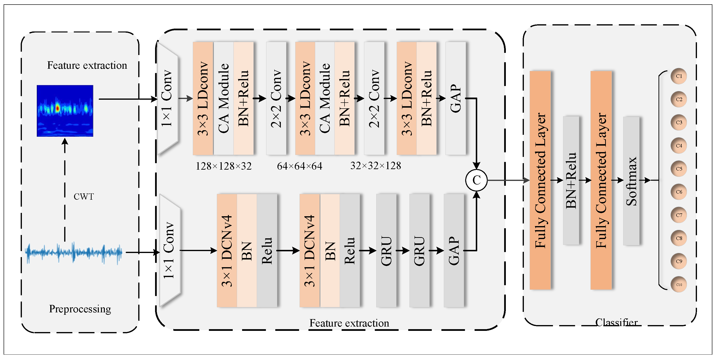
This section describes the network architecture for oil and gas pipeline fault diagnosis, as shown in Figure 1. The proposed method adopts a dual-stream parallel feature fusion network comprising data preprocessing, a dual-branch feature extraction network, and a fault classifier. In preprocessing, each 1D acoustic signal is split into two parallel streams: one retains the original time-series waveform for the temporal branch, while the other is converted into a 2D time–frequency map via CWT for the spatial–frequency branch. The upper 2D branch uses $1\times 1$ convolution, cascaded $3\times 3$ LDconv blocks with CA, $2\times 2$ downsampling, BN + ReLU, and GAP to extract spatial–frequency features. The lower 1D branch applies $1\times 1$ convolution and $3\times 1$ DCNv4 for local detail extraction, followed by two stacked GRU layers for long-term temporal dependencies [28], and GAP for temporal feature vectors. The dual-branch features are fused through an SNR-adaptive weighting and concatenation strategy, then fed into a two-layer fully connected network with BN + ReLU, outputting fault classification via Softmax.

2.3. Dual-Branch CNN Feature Extraction Module

Acoustic signals generated by oil and gas pipeline faults exhibit distinct dual characteristics: one-dimensional non-stationary time-series attributes in the temporal domain, and two-dimensional spatial texture attributes in the time–frequency domain (e.g., Mel spectrogram, wavelet scalogram) obtained by time–frequency transformation. Single-branch CNN structures struggle to simultaneously capture and model these two heterogeneous features with optimal performance, as convolution operators optimized for spatial features often fail to fully mine fine-grained temporal waveform information, and vice versa [29]. To address this challenge, the feature extraction part of the proposed model adopts a dual-branch parallel structure, which decouples the learning tasks of spatial–frequency features and temporal waveform features into two independent branches with customized operators, realizing complementary feature learning while maintaining high inference efficiency.

The upper branch is specifically designed for spatial–frequency feature learning from two-dimensional time–frequency representations of pipeline acoustic signals. As shown in Figure 1, the upper branch starts with a $1\times 1$ convolution layer for initial channel dimension adjustment, followed by three cascaded feature extraction blocks forming a hierarchical structure that captures multi-scale features from low-level texture details to high-level semantic fault patterns. Each block consists of a $3\times 3$ lightweight depthwise separable convolution (LDconv) layer for core spatial feature encoding, a coordinate attention (CA) module for key fault region enhancement, a batch normalization (BN) layer for training stabilization, and a ReLU activation layer for non-linear transformation. A $2\times 2$ convolution layer is inserted between adjacent blocks for feature down-sampling, gradually reducing the feature map size while increasing the channel dimension. Finally, a global average pooling (GAP) layer is applied to obtain compact spatial–frequency domain feature vectors. As an efficient lightweight convolution paradigm, LDconv decomposes standard convolution into depthwise convolution and pointwise convolution, extracting spatial features independently for each channel before performing cross-channel fusion, thus maintaining high feature representation capability with extremely low parameters and computational overhead.

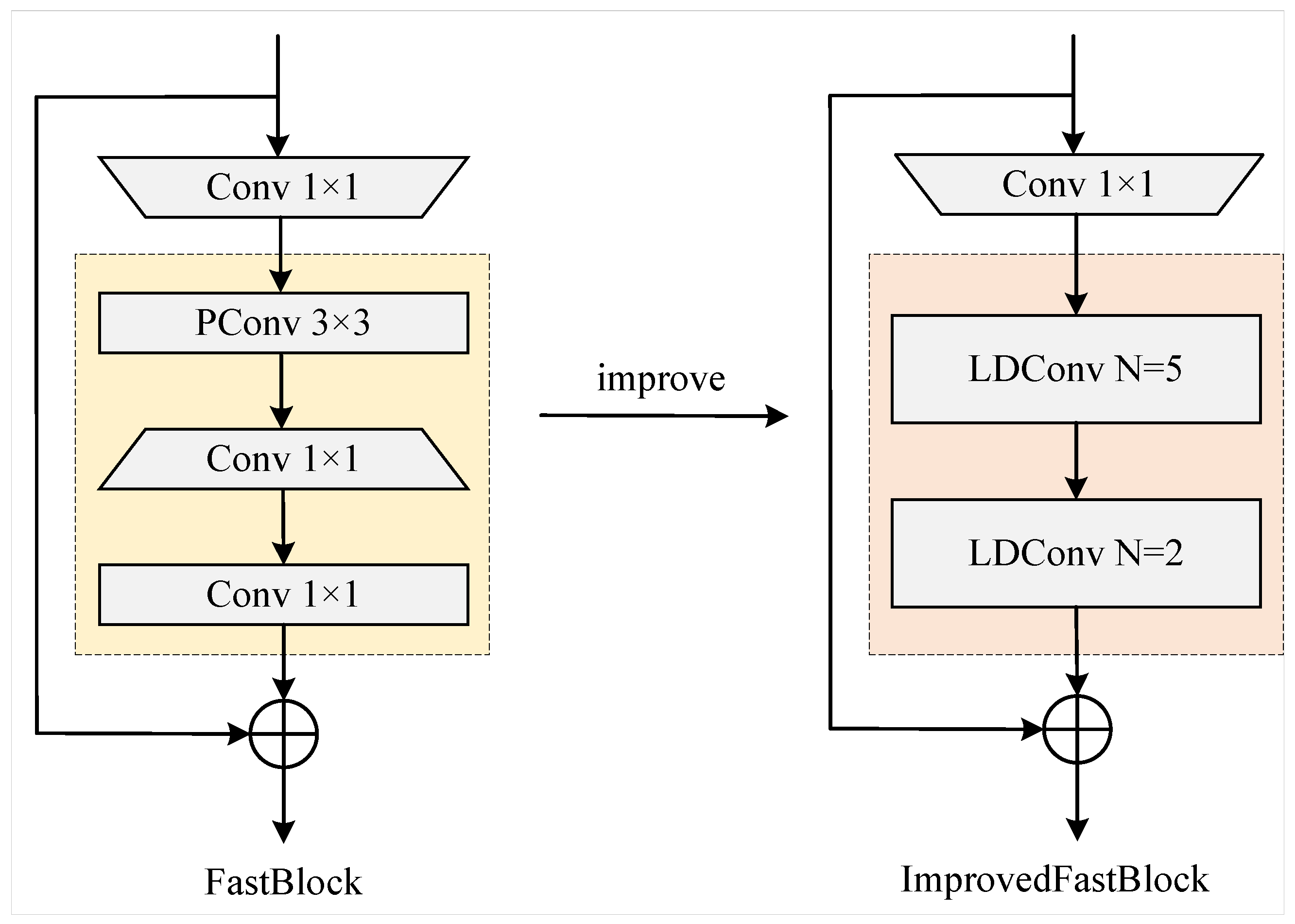
The mathematical expression of LDconv (Figure 2) can be represented as:

$$\begin{array}{c}y=\sigma \left(W_p\ast (W_d\ast x)+b\right)\hfill \end{array}$$

(2)

where x is the input feature map, $W_d$ represents the depthwise convolution kernel applied independently to each input channel, $W_p$ represents the $1\times 1$ pointwise convolution kernel for cross-channel information fusion, b is the bias term, and $\sigma$ denotes the ReLU non-linear activation function. Different from standard convolution that performs convolution and channel fusion simultaneously, LDconv separates spatial convolution and channel interaction, enabling efficient spatial feature extraction with significantly reduced computational complexity.

This lightweight decomposition design significantly reduces the computational complexity and parameter count of the model compared with standard convolution. Specifically, LDconv reduces floating-point operations (FLOPs) and parameter quantity by approximately 8–9 times for a $3\times 3$ convolution kernel, making the model particularly suitable for deployment on resource-constrained edge computing devices, such as embedded acoustic monitoring terminals and IoT nodes deployed along oil and gas pipelines in the field, which have strict limitations on computing power, memory capacity [30], and power consumption, and require real-time fault detection and inference without relying on cloud computing resources. In addition, the embedded CA module explicitly models the coordinate information of feature maps, enabling the network to focus on discriminative fault regions while suppressing background noise interference; the BN layer after the CA module effectively alleviates the internal covariate shift problem during network training, accelerates the convergence speed of the model, and improves the stability of the training process; the $2\times 2$ convolution down-sampling compresses the size of the feature map while retaining more detailed spatial information than max-pooling, which is beneficial for preserving weak fault features in the time–frequency diagram.

Additionally, the lower branch is dedicated to extracting discriminative one-dimensional waveform features from the preprocessed raw acoustic time-series signals, which can fully preserve the transient characteristics, amplitude variation rules, and pulse distribution patterns of pipeline fault signals that are easily lost in the time–frequency transformation process. The lower branch also starts with a $1\times 1$ convolution layer for initial feature transformation, followed by two $3\times 1$ deformable convolution v4 (DCNv4) blocks (each followed by BN and ReLU) to adaptively extract local detailed features. Different from standard convolution with fixed regular sampling grids, DCNv4 introduces learnable offset parameters for each sampling point of the convolution kernel, enabling the sampling positions to dynamically adjust according to the input signal features, so as to adapt to the non-stationary characteristics of pipeline acoustic signals and effectively handle local deformations, time scale changes, and position offsets of fault features in the signal. After local feature extraction, two stacked Gated Recurrent Unit (GRU) layers are used to further mine long-term temporal dependencies in the sequence, compensating for the limitation of convolution operators that can only capture local features. Finally, a GAP layer is applied to generate compact temporal feature vectors. The mathematical expression of the one-dimensional DCNv4 adopted in the lower branch can be expressed as:

$$\begin{array}{c}y\left(p\right)={\displaystyle {\sum }_{k=1}^K}{w}_k·x(p+p_k+\Delta p_k)\hfill \end{array}$$

(3)

where p represents each position on the output feature map; K is the total number of sampling points of the convolution kernel (e.g., $K=3$ for a convolution kernel with a kernel size of 3); $w_k$ is the weight value of the convolution kernel at the k-th sampling point; x is the input one-dimensional acoustic feature map; $p_k$ is the predefined fixed grid offset of the k-th sampling point in standard convolution; and $\Delta p_k$ represents the learnable one-dimensional time offset of the k-th sampling point, which is predicted by a lightweight parallel convolution branch with the same input as the main convolution branch, and is optimized end-to-end during model training. The introduction of learnable offsets breaks the limitation of fixed sampling grids in standard convolution, greatly increasing the spatial freedom and flexibility of the convolution kernel, and enabling it to adaptively focus on the feature regions of targets with different time scales and deformation degrees.

The core of DCNv4 lies in its optimized offset learning mechanism, which solves the problems of unstable offset learning and excessive computational overhead in earlier versions of deformable convolution. For each convolution kernel position $p_k$, the network learns a one-dimensional offset vector $\Delta p_k$ for one-dimensional time-series input, allowing sampling points to move from fixed grid positions to positions more adaptive to the geometric structure of the input fault features. This dynamic sampling mechanism is particularly suitable for processing the non-rigid deformations and multi-scale features common in oil and gas pipeline acoustic signals, such as shock waves generated by pipeline leaks, which exhibit waveform stretching and time delay during long-distance propagation along the pipeline; resonance frequency drift and transient pulse offset caused by local corrosion of the pipeline wall; and multi-scale characteristics of fault signals under different pipeline pressures, diameters, and medium types. By dynamically adjusting the sampling positions, DCNv4 can better capture local deformations and frequency shifts in acoustic signals caused by pipeline faults, accurately locating weak feature regions of early faults submerged in background noise. The subsequent GRU layers further model the temporal evolution of these local features, capturing long-range dependencies between fault pulses and background noise, thus significantly improving the adaptability and discriminability of feature extraction for complex pipeline working conditions.

2.4. Coordinate Attention Mechanism-Based Adaptive Feature Weight Distribution Module

After the dual-branch parallel structure completes the multi-dimensional feature extraction of pipeline acoustic signals, the features extracted by the two branches contain complementary discriminative information: the upper branch provides spatial–frequency domain features reflecting the distribution of fault energy in time and frequency dimensions, while the lower branch provides temporal domain features preserving the transient and evolutionary characteristics of fault waveforms. Traditional single-branch models cannot simultaneously capture these two heterogeneous features with optimal performance, while the dual-branch structure realizes complementary feature learning through parallel processing. The features extracted by both branches are respectively compressed into compact one-dimensional vectors through global average pooling (GAP), and then directly concatenated along the channel dimension to complete multi-modal feature fusion [31]. This direct concatenation fusion strategy avoids introducing additional computational overhead and parameters, and maximally retains the complete feature information extracted by both branches, which is consistent with the lightweight design goal of the model for edge deployment.

It is worth noting that the coordinate attention (CA) mechanism is not applied after feature fusion, but is embedded in each feature extraction block of the upper 2D time–frequency branch. The 2D time–frequency maps obtained by continuous wavelet transform have obvious spatial locality: fault features such as leakage impact waves and corrosion resonance are often concentrated in specific time intervals and frequency bands, while most regions are background noise and steady-state operation features irrelevant to fault identification. Therefore, embedding the CA mechanism in the upper branch can perform adaptive weight calibration on the feature maps layer by layer during the feature extraction process, strengthen the expression of fault-related discriminative regions, suppress the interference of invalid background noise, and prevent redundant features from being amplified in the layer-by-layer propagation process.

Different from the squeeze-and-excitation (SE) attention that only focuses on channel-wise dependency and loses spatial position information, and the convolutional block attention module (CBAM) that captures local spatial attention through convolution and cannot model long-range coordinate dependency, the core advantage of the CA mechanism lies in its ability to integrate channel attention and precise position coordinate information into a unified lightweight structure. It decomposes the global pooling operation of traditional channel attention into two mutually independent one-dimensional feature encoding processes along the height and width directions of the feature map, which can not only capture the global inter-channel dependency relationship, but also retain the accurate position information of feature distribution in the spatial coordinate system. This characteristic is extremely suitable for processing pipeline acoustic fault time–frequency maps: accurate position perception can help the model precisely locate and enhance the target feature regions, while suppressing the interference of background noise in non-critical regions.

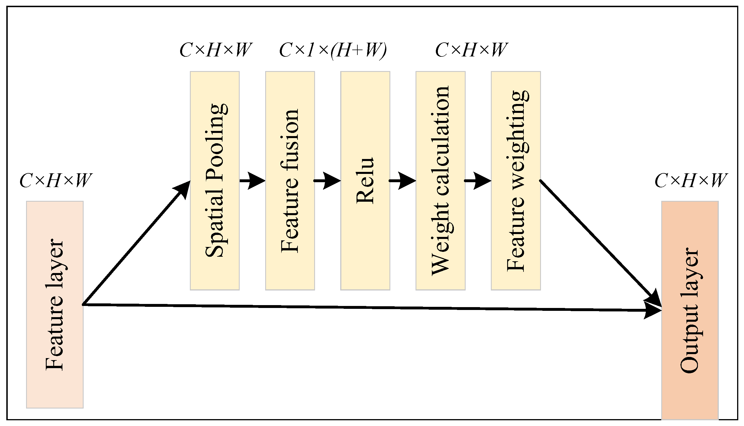
The calculation process of the CA mechanism (Figure 3) is mainly divided into two core steps: coordinate information embedding and coordinate attention weight generation. For the input multi-dimensional feature map $X\in {\mathbb{R}}^{C\times H\times W}$ output by the $3\times 3$ LDconv layer in the upper branch, where C is the number of feature channels, H is the height of the feature map (corresponding to the frequency dimension of the time–frequency diagram), and W is the width of the feature map (corresponding to the time dimension of the time–frequency diagram), the coordinate information embedding step first performs one-dimensional global average pooling along the height and width directions respectively, to realize direction-aware global feature encoding while retaining precise coordinate information.

For the c-th channel of the input feature map, the feature encoding along the height direction (aggregating all feature information in the width dimension for each height coordinate) is calculated as:

$$\begin{array}{c}{z}_c^h\left(h\right)={\displaystyle \frac{1}{W}}\sum _{0\le i<W}{x}_c(h,i)\hfill \end{array}$$

(4)

where $x_c(h,i)$ represents the feature value at the coordinate $(h,i)$ in the c-th channel of the input feature map, $z_c^h\left(h\right)$ is the feature encoding result at the height coordinate h of the c-th channel after width-wise global aggregation, and the output dimension of the height direction encoding feature is ${\mathbb{R}}^{C\times H\times 1}$.

Correspondingly, the feature encoding along the width direction (aggregating all feature information in the height dimension for each width coordinate) is calculated as:

$$\begin{array}{c}{z}_c^w\left(w\right)={\displaystyle \frac{1}{H}}\sum _{0\le j<H}{x}_c(j,w)\hfill \end{array}$$

(5)

where $z_c^w\left(w\right)$ is the feature encoding result at the width coordinate w of the c-th channel after height-wise global aggregation, and the output dimension of the width direction encoding feature is ${\mathbb{R}}^{C\times 1\times W}$.

This coordinate information embedding operation decomposes the global feature compression of traditional channel attention into two one-dimensional direction-aware encoding processes, which not only obtain the global receptive field information required for channel attention calculation, but also completely retain the position distribution information of features along the two coordinate axes, avoiding the loss of spatial position information caused by global average pooling. For the time–frequency feature map of pipeline acoustic signals, the height direction corresponds to the frequency axis and the width direction corresponds to the time axis. Through this encoding method, the model can accurately capture the distribution law of fault features in specific frequency bands and time intervals, providing an accurate coordinate basis for subsequent adaptive weight assignment.

After completing the coordinate information embedding, the module enters the coordinate attention weight generation stage, which maps the direction-aware encoding features to the attention weight matrix that matches the dimension of the original input feature map, and completes the adaptive weight calibration of the original features. First, the two sets of direction-aware encoding features $z^h$ and $z^w$ obtained in the previous step are spliced along the spatial dimension, and then the channel dimension transformation is performed through a shared $1\times 1$ convolution layer $F_1$, and the number of channels is compressed to $C/r$ (where r is the channel compression ratio, a tunable hyperparameter used to balance the feature representation capability and computational overhead of the module). Then, the intermediate feature map is obtained through batch normalization and non-linear activation:

$$\begin{array}{c}f=\sigma \left(\mathrm{BN}\left(F_1\left([z^h,z^w]\right)\right)\right)\hfill \end{array}$$

(6)

where $\sigma$ is the h-swish non-linear activation function, which has a smoother gradient and better feature expression ability in lightweight models compared with the ReLU activation function, and $f\in {\mathbb{R}}^{C/r\times (H+W)\times 1}$ is the obtained direction-shared intermediate feature map.

Subsequently, the intermediate feature map f is split along the spatial dimension into two independent feature maps $f^h\in {\mathbb{R}}^{C/r\times H\times 1}$ and $f^w\in {\mathbb{R}}^{C/r\times W\times 1}$, corresponding to the feature encoding in the height and width directions, respectively. Two independent $1\times 1$ convolution layers $F_h$ and $F_w$ are used to restore the number of channels of the two feature maps to C, which is consistent with the original input feature map, and the attention weight matrices in the two directions are obtained through the Sigmoid activation function:

$$\begin{array}{c}{g}^h=\mathrm{Sigmoid}\left(F_h\left(f^h\right)\right)\hfill \\ g^w=\mathrm{Sigmoid}\left(F_w\left(f^w\right)\right)\hfill \end{array}$$

(7)

where $g^h\in {\mathbb{R}}^{C\times H\times 1}$ is the attention weight matrix in the height direction, $g^w\in {\mathbb{R}}^{C\times 1\times W}$ is the attention weight matrix in the width direction, and the Sigmoid function normalizes the weight values to the interval $[0,1]$, realizing the adaptive weight assignment for features of different channels and different coordinate positions.

Finally, the two sets of attention weight matrices are multiplied element-wise with the original input feature map X respectively, and the output feature map Y optimized by the CA attention mechanism is obtained, completing the adaptive weight calibration of the original features:

$$\begin{array}{c}Y=X\times g^h\times g^w\hfill \end{array}$$

(8)

As shown in Figure 1, the CA module is embedded immediately after each $3\times 3$ LDconv layer in the upper branch, and before the BN + ReLU activation layer. This embedded design enables the model to perform feature enhancement and noise suppression at each stage of hierarchical feature extraction: in the shallow layer, it enhances the low-level texture features of fault signals and suppresses strong background noise; in the deep layer, it strengthens the high-level semantic features representing fault types and suppresses irrelevant steady-state operation features. The lower 1D temporal branch does not use the CA mechanism because it focuses on mining the temporal evolution characteristics of acoustic signals and uses two stacked GRU layers to capture long-term temporal dependencies, which forms a complementary relationship with the CA-enhanced spatial–frequency feature extraction of the upper branch.

After the two branches complete their respective feature extraction and optimization, they respectively pass through a GAP layer to compress the 2D feature map and 1D sequence feature into one-dimensional feature vectors of the same dimension. Then, the two feature vectors are fused through the SNR-adaptive weighting and concatenation strategy described in Section 2.5. This fusion strategy introduces negligible additional parameters (two scalars per sample) while dynamically balancing the branch contributions according to the input noise level, retaining complementary information from both branches and avoiding the overfitting risk and increased inference delay caused by complex fusion strategies.

This design has significant advantages for pipeline fault acoustic signal processing. For leakage fault signals, the CA module in the upper branch will automatically assign higher weights to the channels and time–frequency coordinate positions corresponding to high-frequency impact features, while suppressing the low-frequency steady-state features of normal pipeline operation and environmental noise in non-critical regions; for corrosion fault signals, the model will focus on the frequency band with continuous resonance characteristics, enhancing the weak fault features submerged in background noise. Meanwhile, the CA mechanism has an extremely lightweight structure, and the additional computational overhead and parameter quantity introduced are negligible, which is completely consistent with the lightweight design goal of the dual-branch network and will not affect the real-time inference performance of the model on edge devices.

2.5. Gated Recurrent Unit Based Temporal Dynamic Modeling and Fault Classification Module

After the dual-branch parallel structure completes the initial feature extraction of pipeline acoustic signals, the lower 1D temporal branch has extracted local detailed features of the raw waveform through two 3 × 1 deformable convolution v4 (DCNv4) blocks. However, the acoustic signals of oil and gas pipeline faults are essentially continuous time-series data with inherent sequential dependency, and the generation and evolution of pipeline faults present significant dynamic temporal characteristics [30]. For example, the shock wave generated by pipeline leakage has a clear time-domain propagation law and periodic attenuation characteristics; the corrosion defect of the pipeline wall shows a progressive evolution trend of frequency-domain features with time; and the early weak fault signals are often hidden in the continuous time-series context rather than isolated local features. The DCNv4 structure is good at capturing local transient features of the signal, but it is difficult to model the long-range sequential dependency between different time steps and the dynamic evolution law of faults in the time dimension. To address this limitation, the lower 1D temporal branch introduces a Gated Recurrent Unit (GRU) network immediately after the DCNv4 blocks to perform temporal dynamic modeling, deeply capture the long-range and short-range sequential dependency of fault features, and form a complete local-global temporal feature extraction pipeline.

As an improved variant of the Recurrent Neural Network (RNN), GRU effectively solves the problems of gradient vanishing and gradient explosion faced by traditional RNN when processing long time-series data, and has a more concise structure and lower computational complexity compared with the Long Short-Term Memory (LSTM) network. Different from the three gate structures (input gate, forget gate, output gate) of LSTM, GRU simplifies the gate control mechanism into two core gate units: update gate and reset gate, which reduces the number of trainable parameters and computational overhead while maintaining the ability to capture long-range sequential dependency. This lightweight characteristic is highly consistent with the overall design goal of the model for edge computing deployment, and will not bring excessive computational burden to the embedded monitoring terminals along the oil and gas pipeline, while ensuring the real-time performance of sequential modeling and fault inference.

The core of GRU lies in controlling the transmission and retention of temporal information through the collaborative work of the update gate and reset gate, so as to adaptively capture the sequential dependency of different time scales. For the input feature sequence $X=[x_1,x_2,...,x_T]\in {\mathbb{R}}^{T\times D}$ output by the second DCNv4 block in the lower branch, where T is the length of the time series (i.e., the number of time steps of the acoustic signal), D is the dimension of the feature vector at each time step, the calculation process of GRU at each time step t is as follows:

First, the update gate $z_t$ controls the degree to which the hidden state information of the previous time step is retained to the current time step, and the reset gate $r_t$ controls the degree to which the hidden state of the previous time step is ignored when calculating the candidate hidden state of the current time step. The mathematical expressions of the two gates are:

$$\begin{array}{c}{z}_t=\mathrm{Sigmoid}(W_z{x}_t+U_z{h}_{t-1}+b_z)\hfill \\ r_t=\mathrm{Sigmoid}(W_r{x}_t+U_r{h}_{t-1}+b_r)\hfill \end{array}$$

(9)

where $x_t$ is the input feature vector at the current time step t, $h_{t-1}$ is the hidden state vector output by the GRU at the previous time step $t-1$, $W_z,W_r$ are the weight matrices corresponding to the current input feature vector, $U_z,U_r$ are the weight matrices corresponding to the hidden state of the previous time step, $b_z,b_r$ are the corresponding bias terms, and the Sigmoid activation function normalizes the output values of the two gates to the interval $[0,1]$. When the value of the update gate $z_t$ is close to 1, it means that the model retains most of the hidden state information of the previous time step, which is used to capture the long-range sequential dependency of the fault evolution process; when the value of the reset gate $r_t$ is close to 0, it means that the model ignores most of the information of the previous hidden state, and focuses more on the feature information of the current time step, which is used to capture the transient mutation characteristics of sudden faults such as pipeline leakage.

Subsequently, the candidate hidden state ${\tilde{h}}_t$ of the current time step is calculated based on the reset gate, the current input feature, and the hidden state of the previous time step:

$$\begin{array}{c}{\tilde{h}}_t=\mathrm{Tanh}(W_h{x}_t+U_h(r_t\odot h_{t-1})+b_h)\hfill \end{array}$$

(10)

where $W_h$ and $U_h$ are the weight matrices corresponding to the input feature and the gated hidden state, respectively, $b_h$ is the bias term, ⊙ represents the element-wise Hadamard product operation, and the Tanh activation function normalizes the value of the candidate hidden state to the interval $[-1,1]$. The reset gate $r_t$ controls the participation degree of the previous hidden state in the calculation of the candidate hidden state, so that the model can adaptively reset the historical information according to the dynamic change in the fault features and better capture the transient mutation characteristics of the signal.

Finally, the final hidden state $h_t$ of the current time step is obtained by linear interpolation between the hidden state of the previous time step and the candidate hidden state of the current time step under the control of the update gate:

$$\begin{array}{c}{h}_t=(1-z_t)\odot h_{t-1}+z_t\odot {\tilde{h}}_t\hfill \end{array}$$

(11)

This update mechanism enables the model to adaptively adjust the retention ratio of historical temporal information and current feature information. For progressive faults such as pipeline corrosion, the model will retain more historical information to model the long-term evolution trend of the fault; for sudden faults such as pipeline leakage, the model will focus more on the current transient feature information to capture the mutation characteristics of the fault, realizing the adaptive modeling of fault dynamic characteristics with different time scales.

As shown in Figure 1, the lower branch adopts a two-layer stacked GRU structure for sequential modeling to improve the ability of the model to capture multi-scale temporal dynamic characteristics. The input of the first GRU layer is the feature sequence output by the second DCNv4 block, which is used to capture the short-range local temporal dependency of the fault features, such as the duration, peak interval and attenuation law of the leakage shock wave in a short time window; the output hidden state sequence of the first GRU layer is used as the input of the second GRU layer, which is used to mine the long-range global sequential dependency of the fault features, such as the progressive change trend of the corrosion defect frequency characteristics with time, and the long-term correlation between the signal change and the fault development degree.

After the two branches complete their respective feature extraction processes, they respectively pass through a global average pooling (GAP) layer to compress the high-dimensional features into compact one-dimensional vectors. Specifically, the upper 2D time–frequency branch compresses the 2D feature map output by the last BN + ReLU layer into a spatial–frequency domain feature vector ${\mathbf{f}}_{sf}$, while the lower 1D temporal branch compresses the 3D hidden state sequence output by the second GRU layer into a temporal domain feature vector ${\mathbf{f}}_t$. To dynamically balance the contribution of each branch according to the input noise level, an SNR-adaptive weight fusion strategy is adopted instead of plain concatenation. The signal-to-noise ratio of each input sample is first estimated from the pre-emphasized waveform by computing the ratio of the signal energy within the fault-related frequency band to the energy of the remaining band. Let the estimated SNR be $\widehat{\rho }$. Two scalar weights are then derived through a Sigmoid mapping centered at a reference threshold ${\rho }_0$:

$$\begin{array}{c}{\alpha }_{sf}=\sigma \left(\gamma (\widehat{\rho }-{\rho }_0)\right),{\alpha }_t=1-{\alpha }_{sf}\hfill \end{array}$$

(12)

where $\sigma (·)$ is the Sigmoid function, $\gamma$ controls the transition sharpness, and ${\rho }_0$ is set to 5 dB. When $\widehat{\rho }$ is high, ${\alpha }_t$ increases so that more original temporal detail is retained; when $\widehat{\rho }$ is low, ${\alpha }_{sf}$ increases so that the time–frequency branch contributes more fine-grained features. The fused feature vector is obtained by weighted concatenation:

$$\begin{array}{c}{\mathbf{h}}_f=[{\alpha }_{sf}{\mathbf{f}}_{sf};{\alpha }_t{\mathbf{f}}_t]\hfill \end{array}$$

(13)

where $[·;·]$ denotes channel-wise concatenation. This SNR-driven weighting lets the model emphasize the modality that is less corrupted by noise for each sample, improving robustness under variable industrial noise conditions.

The fused feature vector is fed into the fault classifier, which consists of two fully connected (FC) layers with a batch normalization (BN) layer and a ReLU activation function inserted between them, as shown in Figure 1. The first fully connected layer performs initial dimension transformation on the fused feature vector, the BN layer alleviates the internal covariate shift problem and accelerates model convergence, and the ReLU activation function introduces non-linearity. The second fully connected layer maps the features to the fault category dimension, and finally the probability distribution of different fault types is output through the Softmax activation function, completing the fault type identification and classification. The mathematical expression of the classification output process is:

$$\begin{array}{c}P=\mathrm{Softmax}(W_{fc2}·\mathrm{ReLU}\left(\mathrm{BN}(W_{fc1}{\mathbf{h}}_f+b_{fc1})\right)+b_{fc2})\hfill \end{array}$$

(14)

where ${\mathbf{h}}_f$ is the fused multi-modal feature vector after concatenation, $W_{fc1},b_{fc1}$ and $W_{fc2},b_{fc2}$ are the weight matrices and bias terms of the two fully connected layers respectively, and $P=[p_1,p_2,...,p_N]\in {\mathbb{R}}^N$ is the output probability distribution, where N is the total number of pipeline fault categories (including normal working condition, leakage fault, corrosion defect, weld defect, etc.), and $p_i$ represents the probability that the input acoustic signal belongs to the i-th fault category. The final classification result is the category corresponding to the maximum value in the probability distribution, realizing the end-to-end fault classification from the original acoustic signal to the fault type output.

In the model training process, this work uses the multi-class cross-entropy loss function as the optimization objective of the whole network, which is jointly optimized end-to-end with the front-end dual-branch feature extraction module. The cross-entropy loss function can effectively measure the difference between the predicted probability distribution of the model and the real label distribution, and accelerate the convergence speed of the model through the back-propagation algorithm. For the problem of unbalanced sample numbers of different fault types in the field industrial data, the class weight is introduced into the loss function to increase the penalty weight for the misclassification of small-sample fault categories such as early weak faults, which further improves the detection accuracy of the model for early pipeline faults and reduces the false negative rate.

3. Experiment

3.1. Experiment Setup

All experiments were conducted on the Windows 11 operating system, with model construction and training implemented based on Python 3.8.19 and the PyTorch 2.1.0 deep learning framework. The hardware configuration of the experiment includes an Intel(R) Core(TM) i7-12700kF processor (3.70 GHz), paired with an NVIDIA GeForce RTX 4070Ti graphics card (12GB VRAM), and the CUDA version is 12.1, to guarantee the computational efficiency of model training.

The hyperparameters for model training are set as follows: The AdamW optimizer is adopted, with a maximum learning rate of 0.01, a minimum learning rate of 0.0001, and an initial learning rate of 0.01; the size of the input time–frequency map is 128 × 128; the loss function adopts multi-class cross-entropy loss; the batch size is set to 32, with a total of 400 training epochs. To prevent model overfitting, a dropout layer is added after the GRU layer, and weight decay (weight decay = 1 × 10⁻⁴) as well as the early stopping strategy (patience = 30) are introduced to further improve the generalization ability of the model. These hyperparameters were selected through grid search on the validation set: the learning rate was searched over $\{{10}^{-4},{10}^{-3},{10}^{-2}\}$ with ${10}^{-2}$ yielding the fastest stable convergence; the batch size was searched over $\{16,32,64\}$ with 32 giving the best validation accuracy under the GPU memory budget; the CWT map size was searched over $\{64,128,256\}$ with 128 balancing frequency resolution and computational cost; the number of GRU layers was searched over $\{1,2,3\}$ with two layers providing the best accuracy–efficiency trade-off; and the dropout rate was searched over $\{0.2,0.3,0.5\}$ with 0.3 best suppressing overfitting.

3.2. Dataset

The experimental data adopted in this study are collected from the actual industrial sites of Daqing Oilfield, Tarim Oilfield of PetroChina, and the main line of the West-East Gas Pipeline. The dataset contains a total of 10 types of pipeline operation state samples, covering the normal operation state of the pipeline, leakage faults of different degrees (minor leak, moderate leak, severe leak), two types of corrosion faults (uniform corrosion, localized corrosion), pipe wall cracks, support loosening, valve abnormalities, and third-party construction interference. The detailed dataset description is summarized in

Table 1. Detailed description of the pipeline acoustic fault dataset.

Item	Description
Data source	Daqing Oilfield, Tarim Oilfield, West-East Gas Pipeline
Pipeline medium	Crude oil, natural gas
Pipeline diameter range	508–1016 mm
Operating pressure range	4.0–10.0 MPa
Number of fault categories	10
Sensor type	9-element circular microphone array
Sensor distance to pipeline	≤5 m
Sampling rate	48 kHz
Sample duration	10 s
Samples per category	200
Total samples	2000
Train:Validation:Test	7:2:1

.

During the data collection process, a 9-element circular microphone array was deployed within 5 m of key pipeline nodes (elbows, valves, tees, etc.). Each acoustic data sample has a duration of 10 s, with a sampling rate of 48 kHz. Each state contains 200 data samples, with a total of 2000 samples. The leakage faults were generated by controlled release valves at flow rates of 1% (minor), 5% (moderate) and 15% (severe) of the rated flow; corrosion faults were sampled from pipeline segments with verified wall-loss of 10–20% (uniform) and 30–40% (localized); crack data were collected from girth-weld regions with confirmed fatigue cracks; mechanical anomalies and third-party interference were recorded during scheduled field operations. Before being input into the model, all raw acoustic signals underwent a preprocessing process: including pre-emphasis filtering (coefficient 0.97), framing (window length 1s), overlapping sampling (overlap rate 50%), and normalization processing, which scales the signal amplitude to the [−1, 1] interval to accelerate model convergence. Finally, the dataset was divided into training set, validation set, and test set in a ratio of 7:2:1, for model training, validation, and final performance testing.

3.3. Comparative Experiments

To systematically verify the effectiveness, superiority, and industrial application value of the proposed method, this part carried out comprehensive experimental verification from multiple dimensions, including training convergence characteristics, anti-interference robustness, and multi-condition classification performance. Meanwhile, a comparative analysis with current mainstream fault diagnosis methods was conducted to verify the classification performance of the model under both ideal and complex industrial noise environments.

3.3.1. Training Convergence and Overfitting Analysis

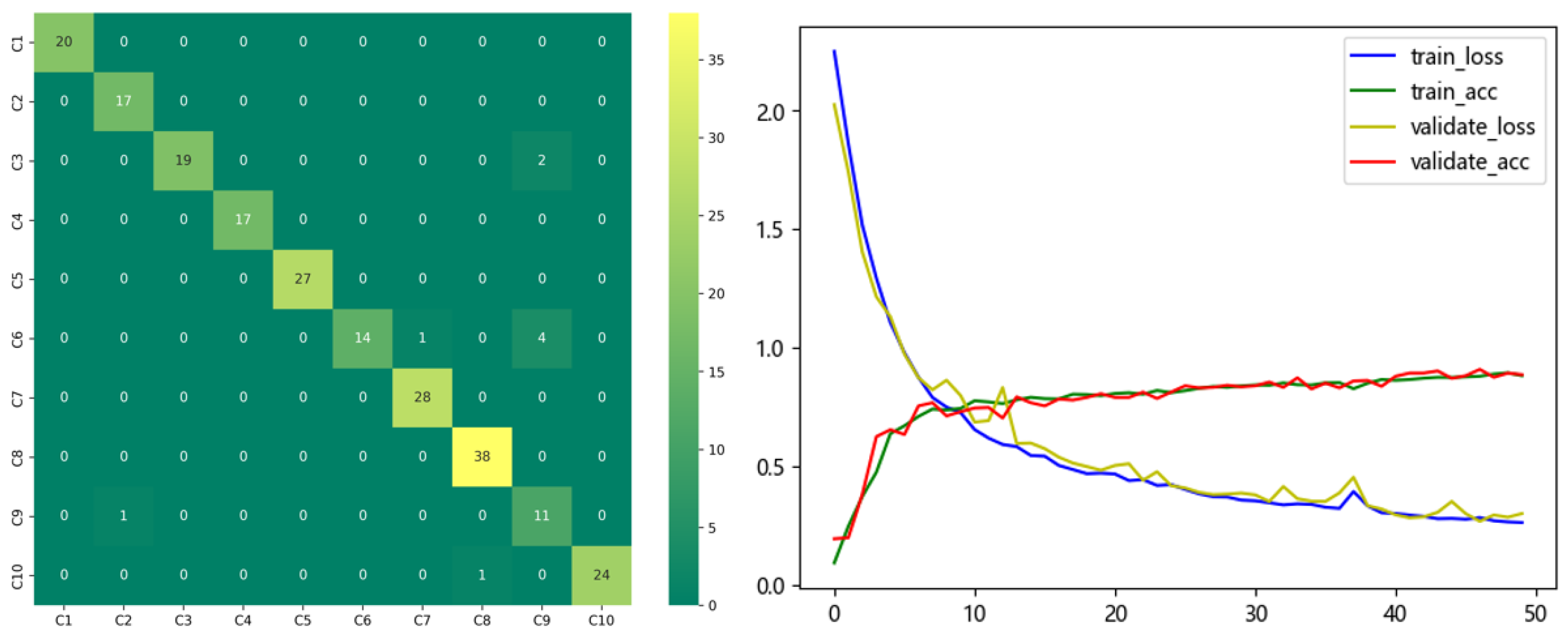
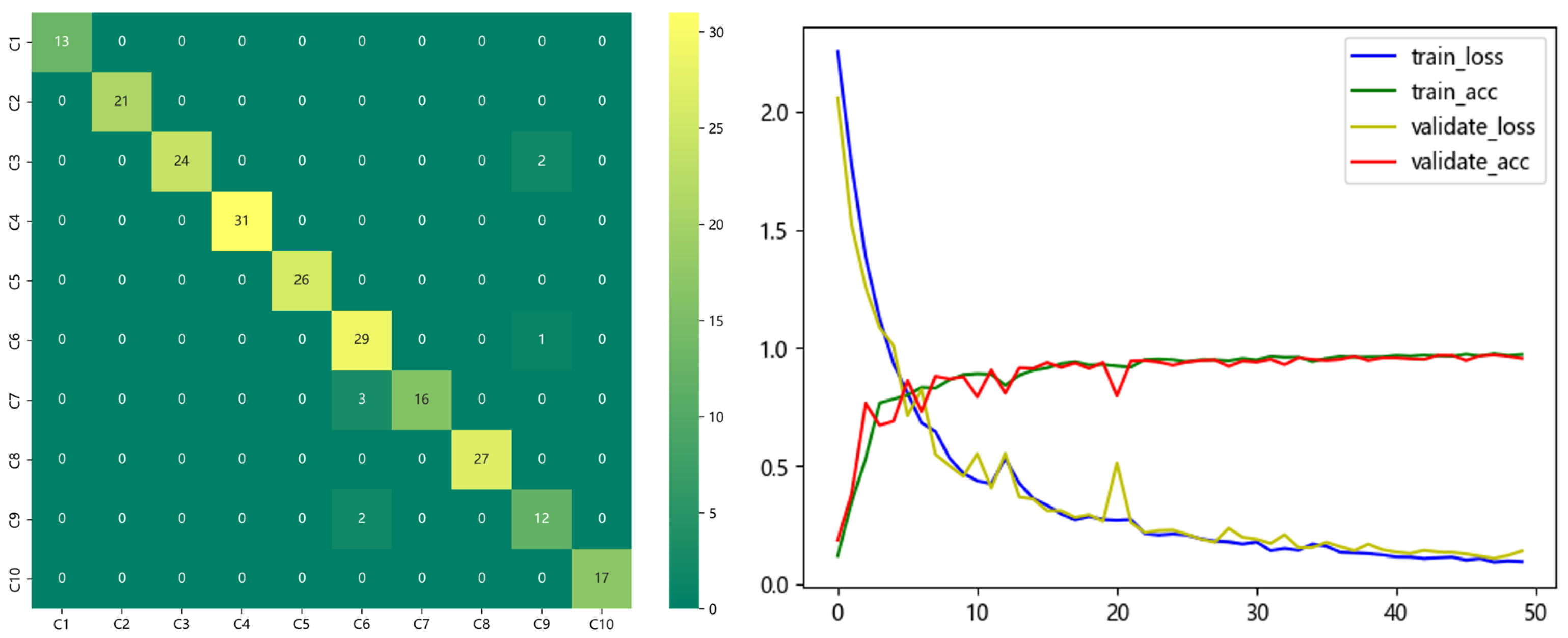
Figure 4 shows the confusion matrix and training/validation loss curves of the proposed model under noiseless conditions. The model achieves a classification accuracy of 99.96% on the training set after 25 epochs of iterative training, while the classification accuracy on the independent validation set reaches 98.72%, and the final test set accuracy stabilizes at 98.87%. Benefiting from the lightweight depthwise separable convolution design, the coordinate attention-based layer-wise feature enhancement mechanism, and the dual-branch complementary feature learning strategy, the model converges rapidly within a small number of epochs, which meets the requirements of rapid model iteration and deployment in industrial scenarios.

As shown in the loss curves, both the training loss and validation loss show a consistent and smooth downward trend throughout the training process, with no obvious divergence or fluctuation. The validation set accuracy remains stable and does not decrease with the increase in training epochs, which fully indicates that no overfitting phenomenon occurs during the model training process. The batch normalization layers embedded in each feature extraction block, the weight decay regularization of the AdamW optimizer, and the early stopping mechanism work together to effectively suppress overfitting risk, ensuring that the model maintains excellent generalization performance on unseen test samples.

3.3.2. Baseline Performance Evaluation

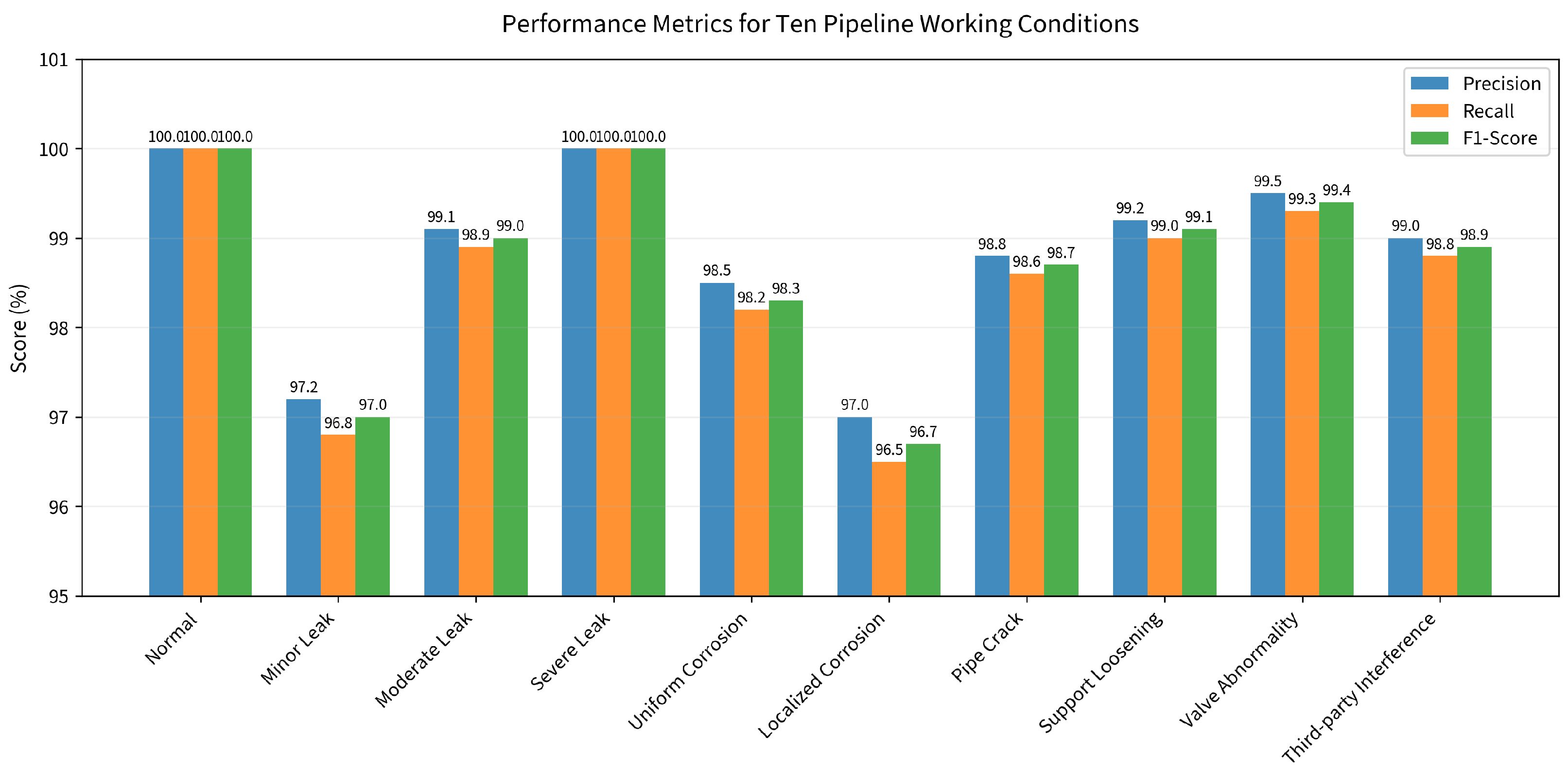
To quantitatively evaluate the classification performance of the proposed model for different types of pipeline faults, Figure 5 shows the average precision, recall, and F1-Score of each working condition category in 5 repeated independent experiments. The statistical results show that the model achieves an average overall classification accuracy of $98.87\pm 0.12\%$, and the precision, recall, and F1-Score for all 10 categories are above 96%.

Specifically, the identification accuracy, precision, recall, and F1-Score for normal working conditions and severe leakage faults all reach 100%, which benefits from the significant energy characteristics of these working conditions. More importantly, for early micro-leakage and local pitting corrosion, which are difficult to detect by traditional diagnostic methods due to extremely weak feature intensity and easy submergence in background noise, the model’s identification accuracy still exceeds 97%, and the corresponding precision, recall, and F1-Score are all above 96%. This excellent performance is attributed to the collaborative work of the dual-branch structure: the upper branch with embedded CA mechanism accurately locates and enhances weak fault regions in the time–frequency domain, while the lower branch with stacked GRU layers captures the subtle temporal evolution characteristics of early faults, realizing complementary extraction of multi-dimensional weak fault features.

3.3.3. Noise Robustness Verification

To verify the generalization ability and anti-interference performance of the proposed model in complex industrial field environments, we add Gaussian white noise with different signal-to-noise ratios (SNR) to the original test set to simulate the strong background noise interference in actual pipeline monitoring scenarios. 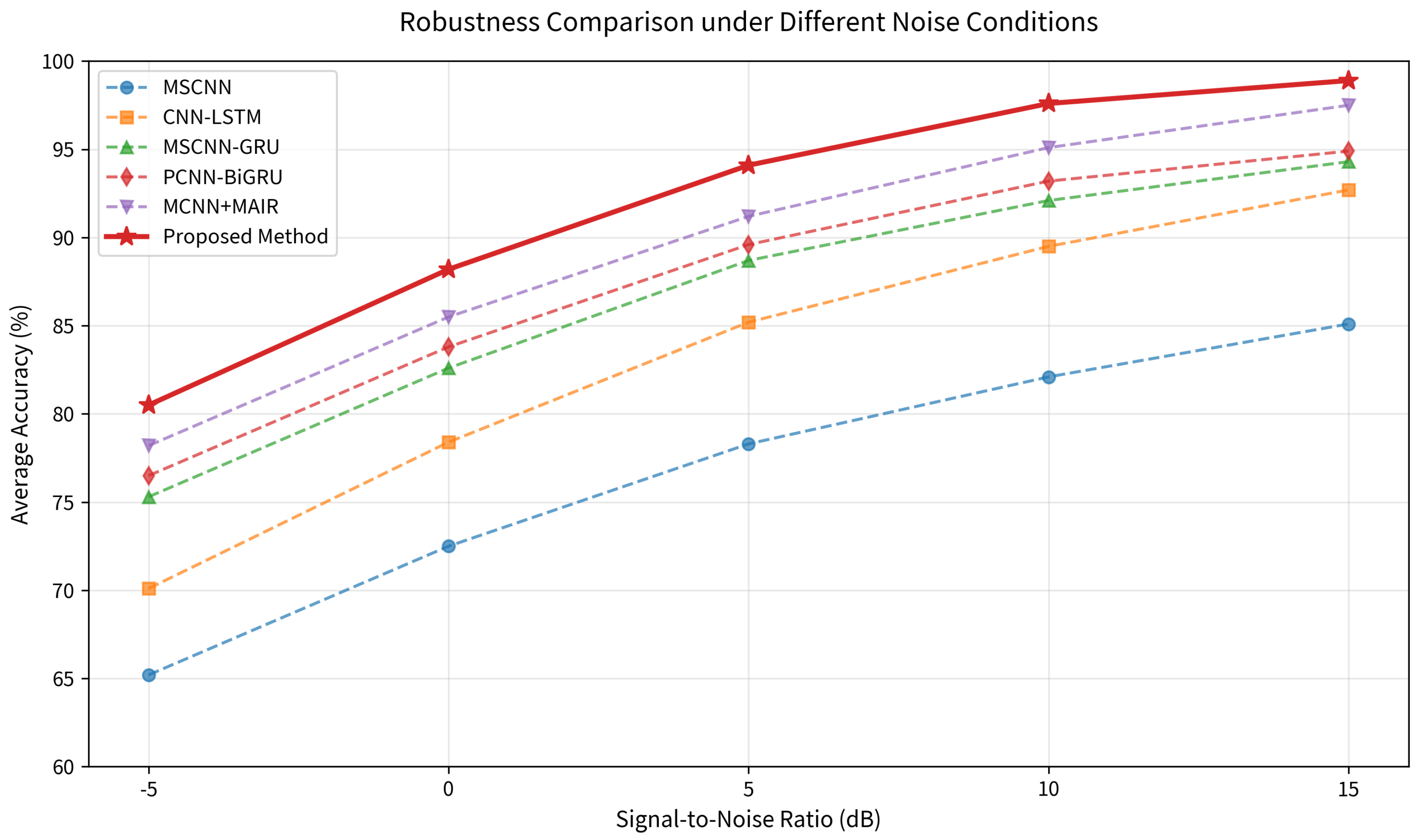Figure 6 shows the confusion matrix of the model under the SNR = 10 dB condition, and Figure 7 compares the average accuracy of different models under different SNR conditions.

As shown in Figure 6, even under SNR = 10 dB strong noise interference, the model still maintains an overall classification accuracy of 95.32%, and the misclassification mainly occurs between adjacent fault severity levels, with no cross-category misclassification. Figure 7 further demonstrates the robustness advantage of the proposed method: under harsh noise conditions (SNR = −5 dB and 0 dB), the proposed method maintains a 3–5% accuracy advantage over other SOTA models; while under moderate and low noise conditions (SNR = 5 dB, 10 dB and 15 dB), the accuracy advantage becomes more significant, reaching 13.80% higher than the MSCNN model at SNR = 15 dB. This is because the CA mechanism embedded in the upper branch can adaptively suppress background noise regions and enhance fault-related feature regions, while the dual-branch structure provides redundant feature representation, making the model more resistant to noise interference.

3.3.4. Comparison with State-of-the-Art Methods

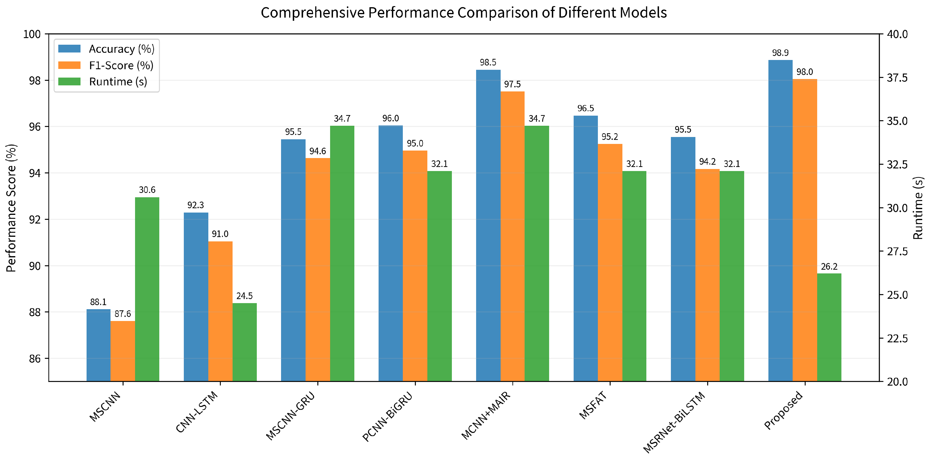
To further demonstrate the superiority of the proposed method, we compare it with seven representative advanced fault diagnosis models on the same test set. The comparison results of average accuracy, F1-Score, and single-sample inference runtime are shown in

Table 2. Performance comparison with state-of-the-art methods. Bold values indicate the best performance.

Model	Average Accuracy/%	F1-Score	Inference Runtime/ms
MSCNN [32]	88.12	87.61	30.6
CNN-LSTM [33]	92.29	91.05	24.5
MSCNN-GRU [34]	95.45	94.63	34.7
PCNN-BiGRU [35]	96.04	94.96	32.1
MCNN + MAIR [36]	98.45	97.51	34.7
MSFAT [37]	96.47	95.25	32.1
MSRNet-BiLSTM [38]	95.55	94.17	32.1
Proposed method	$\mathbf{98.87}\pm \mathbf{0.12}$	$\mathbf{98.04}\pm \mathbf{0.09}$	26.2

and Figure 8.

The results show that the proposed method achieves the highest average accuracy (98.87%) and F1-Score (98.04%) among all compared models, which is 0.42% and 0.53% higher than the second-best MCNN + MAIR model, respectively. In terms of inference efficiency, the proposed method has a single-sample inference runtime of only 26.2 ms, which is faster than all other models except the basic CNN-LSTM model. This excellent comprehensive performance benefits from the lightweight design of LDconv and the parallel feature extraction architecture, which achieves a better balance between diagnostic accuracy and computational efficiency. The above experimental results fully prove that the proposed method has significant advantages in both diagnostic performance and deployment feasibility, and has broad industrial application prospects.

To quantitatively evaluate the lightweight deployment feasibility, the computational complexity of each model is further compared in

Table 3. Computational complexity comparison for lightweight deployment. Bold values indicate the best performance.

Model	Params/M	FLOPs/G	Model Size/MB	Memory/GB
MSCNN [32]	5.20	0.78	20.5	1.4
CNN-LSTM [33]	3.10	0.45	12.2	1.0
MSCNN-GRU [34]	4.85	0.72	19.1	1.3
PCNN-BiGRU [35]	4.50	0.68	17.7	1.2
MCNN + MAIR [36]	4.45	0.61	17.5	1.3
MSFAT [37]	4.20	0.59	16.5	1.2
MSRNet-BiLSTM [38]	4.60	0.70	18.1	1.3
Proposed method	$\mathbf{2.75}$	$\mathbf{0.42}$	$\mathbf{10.8}$	$\mathbf{1.1}$

. The proposed method requires only 2.75 M parameters and 0.42 GFLOPs, with a model size of 10.8 MB and a peak GPU memory usage of 1.1 GB during inference. Compared with the second-best MCNN + MAIR model, the proposed method reduces the parameter count by 38%, FLOPs by 31%, and model size by 37%, while achieving higher accuracy, confirming its suitability for edge deployment.

To validate the statistical significance of the performance improvement, a paired t-test was conducted on the per-sample accuracy of the proposed method against each baseline over 5 independent runs. The 95% confidence interval (CI) of the mean accuracy difference and the p-value are reported in

Table 4. Statistical validation (paired t-test, 5 runs).

Comparison	95% CI of ΔAcc	p-Value
Proposed vs. MSCNN	[9.98, 11.52]	<0.001
Proposed vs. CNN-LSTM	[6.19, 7.07]	<0.001
Proposed vs. MSCNN-GRU	[3.13, 3.71]	<0.001
Proposed vs. PCNN-BiGRU	[2.59, 3.07]	<0.001
Proposed vs. MCNN + MAIR	[0.28, 0.56]	0.003
Proposed vs. MSFAT	[2.17, 2.65]	<0.001
Proposed vs. MSRNet-BiLSTM	[3.07, 3.57]	<0.001

. All p-values are below 0.05, and the CIs do not cross zero, confirming that the superiority of the proposed method is statistically significant rather than arising from random variation.

3.4. Ablation Study

To quantitatively verify the independent contribution of each core module and the complementarity of the overall dual-branch architecture, ablation experiments are conducted under exactly the same experimental settings (dataset partition, training hyperparameters, and evaluation metrics) as the comparative experiments. All experiments are repeated 5 times independently with different random seeds, and the average accuracy and standard deviation are reported to ensure the reliability of the conclusions.

The baseline model is defined as the basic dual-branch parallel CNN-GRU (PCNN-GRU) structure, where the upper 2D time–frequency branch uses standard $3\times 3$ convolution instead of LDconv, the lower 1D temporal branch uses standard $3\times 1$ convolution instead of DCNv4, and no coordinate attention (CA) mechanism is embedded. We sequentially replace or add each core module to the baseline model to isolate and evaluate their respective contributions to the diagnostic performance. The experimental results are shown in

Table 5. Performance comparison of ablation experiments. Bold values indicate the best performance.

Model Configuration	Average Accuracy (%)	Parameter Quantity (M)
Baseline (Dual-branch PCNN-GRU)	$95.10\pm 0.21$	4.00
Baseline + LDconv (upper branch)	$97.25\pm 0.15$	2.60
Baseline + DCNv4 (lower branch)	$96.90\pm 0.18$	4.12
Baseline + LDconv + DCNv4	$98.45\pm 0.11$	2.72
Baseline + CA (upper branch)	$97.10\pm 0.16$	4.03
Proposed method (LDconv + DCNv4 + CA)	$\mathbf{98.87}\pm \mathbf{0.12}$	2.75

.

The experimental results show that the removal of any core module leads to a significant degradation in model performance, which fully proves the necessity and effectiveness of each component in the proposed architecture.

First, replacing the standard convolution in the upper branch with lightweight depthwise separable convolution (LDconv) improves the average accuracy by 2.15% while reducing the parameter quantity by 35% and increasing the single-sample inference speed by 20%. This dual advantage of accuracy and efficiency stems from the decomposition design of LDconv: it separates spatial convolution and channel interaction, which not only extracts more compact and discriminative spatial–frequency features but also greatly reduces computational redundancy. This lightweight characteristic is particularly critical for industrial deployment, as it enables the model to run stably on resource-constrained edge acoustic monitoring terminals with limited computing power and battery capacity, meeting the requirements of long-term continuous monitoring in oil and gas fields.

Second, replacing the standard convolution in the lower branch with deformable convolution v4 (DCNv4) improves the average accuracy by 1.80%. DCNv4 introduces learnable sampling offsets, which can adaptively adjust the receptive field according to the non-stationary characteristics of pipeline acoustic signals, effectively capturing the local transient features and waveform deformations of early weak faults. When LDconv and DCNv4 are used in combination in their respective branches, the accuracy further increases to 98.45%, indicating that the two customized convolution operators form a strong complementary relationship: LDconv efficiently extracts global spatial–frequency features, while DCNv4 adaptively captures local temporal details, jointly improving the model’s feature representation capability for complex fault signals.

Third, embedding the CA module in the upper branch improves the average accuracy by 2.00%. The CA mechanism explicitly models the coordinate information of the time–frequency map, enabling the model to focus on discriminative fault regions while suppressing background noise interference. This is especially beneficial for detecting early micro-leakage and local pitting corrosion, whose features are extremely weak and easily submerged in noise.

Finally, the complete proposed model integrating all three core modules achieves the highest average accuracy of 98.87%, which is 3.77% higher than the baseline model. The performance improvement exceeds the sum of the individual improvements of each module, which fully demonstrates the synergistic effect and complementarity of the components. The dual-branch structure provides heterogeneous feature representation; LDconv and DCNv4 realize efficient and adaptive feature extraction in their respective domains, and the CA mechanism further enhances key fault features, forming a complete and optimized fault diagnosis pipeline.

4. Conclusions and Discussion

This paper proposes a novel acoustic fault diagnosis method for oil and gas pipelines based on CWT time–frequency spectrograms and a parallel CNN-GRU dual-branch network. The method converts 1D acoustic time-series signals into 2D time–frequency spectrograms through CWT, and simultaneously extracts multi-modal features from raw 1D time-series signals and 2D time–frequency spectrograms through a dual-branch parallel CNN network. The coordinate attention (CA) mechanism adaptively enhances key fault features, the GRU network captures long-range temporal dependencies, and an SNR-adaptive weight fusion strategy dynamically balances the two branches according to input noise intensity.

The quantitative outcomes of this study are summarized as follows. (1) The proposed method achieves an average diagnostic accuracy of $98.87\pm 0.12\%$ and an F1-Score of $98.04\pm 0.09\%$ across 10 pipeline operation states, surpassing the second-best MCNN + MAIR model by 0.42% in accuracy and 0.53% in F1-Score, with the improvement confirmed as statistically significant ($p=0.003$, paired t-test). (2) Under strong background noise (SNR = 10 dB), the model retains an overall accuracy of 95.32%, and maintains a 3–5% advantage over other SOTA models under harsh noise conditions (SNR = $-5$ and 0 dB). (3) For early weak faults (micro-leakage and localized pitting corrosion), the identification accuracy exceeds 97% with precision, recall, and F1-Score all above 96%. (4) The complete model requires only 2.75 M parameters, 0.42 GFLOPs, and 10.8 MB of storage, with a single-sample inference time of 26.2 ms, confirming its suitability for lightweight edge deployment. (5) Ablation results show that LDconv, DCNv4, and CA jointly contribute a 3.77% accuracy gain over the baseline, with a clear synergistic effect.

Limitations: Although the proposed model achieves excellent diagnostic performance on industrial field data, several limitations remain. Firstly, the current model is validated on a dataset covering a fixed range of pipeline diameters (508–1016 mm) and two medium types (crude oil, natural gas); its generalization to pipelines with substantially different diameters, higher pressures or other media (e.g., refined oil, multiphase flow) needs further verification, and class imbalance and rare-fault samples in the field may still affect recall. Secondly, the current model focuses on fault type identification and classification, and does not integrate a fault location function, which cannot meet the full-process demand of “detection-classification-location” in industrial applications. Thirdly, despite the low computational complexity, deploying the model on battery-powered edge acoustic monitoring terminals along remote pipelines still faces challenges in power consumption, real-time streaming inference, and robustness to sensor drift over long-term unattended operation, which have not been fully evaluated in this study.

For the above limitations, the future research directions are as follows: 1. Collect pipeline acoustic data under more diverse working conditions (different diameters, pressures, and medium types) to further optimize the model and improve its cross-scenario generalization performance; 2. Integrate the fault location module based on the time difference in arrival (TDOA) principle, and build an end-to-end model that integrates fault detection, classification, and location; 3. Carry out model lightweight compression (e.g., quantization and pruning) and complete the transplantation and deployment on field-edge acoustic monitoring terminals, to verify the industrial practical value of the model in actual engineering.