Protocol and Implementation Sensitivity in Raw-Index-Audited Few-Shot Bearing Fault Diagnosis Benchmarking: Evidence from CWRU and HUSTbearing

Abstract

Sliding-window few-shot evaluations can place support and query windows over shared raw samples. We audited episode-internal overlap, source-noise policy, normalization, and fixed-feature construction using Case Western Reserve University (CWRU) data and a HUSTbearing cross-speed task reconstructed from raw files. In the primary CWRU 0 hp to 3 hp (0 to approximately 2.24 kW), 10-way, 5-shot evaluation at a signal-to-noise ratio (SNR) of −5 dB across 20 seeds, common-pool construction increased log-compressed fast Fourier transform prototype (Log-FFT) accuracy by 3.83 percentage points (95% confidence interval (CI): [+3.63, +4.02]). The corresponding increase for the clean source-supervised cross-entropy prototype encoder (Source-CE-Proto) was 0.95 percentage points and was not statistically distinguishable from zero (95% CI: [−0.004, +1.90]; exact p = 0.05084). Under raw-index-separated evaluation, leave-one-SNR-out Source-CE-Proto achieved 93.23% without direct −5 dB source exposure, compared with 82.43% for Log-FFT. A No-log FFT control achieved 99.09% in the primary task and also exceeded the learned encoders in a second CWRU load pair. HUSTbearing likewise showed channel-dependent fixed-feature accuracy and overlap effects. These results do not support a general method ranking; they support reporting raw-index provenance, source-noise distributions, normalization, and exact feature construction before interpreting method rankings in few-shot bearing fault diagnosis benchmarks.

1. Introduction

Few-shot bearing fault diagnosis addresses settings in which only a small labeled support set is available for a target operating condition. Metric learning, episodic meta-learning, transfer learning, and fixed or learned time-frequency representations have all been used to reduce the dependence on large target-domain training sets [1,2,3,4]. The resulting literature has produced increasingly capable architectures, but a reported accuracy difference is interpretable only if the benchmark controls how raw vibration records are segmented, how support and query sets are formed, what target information is available, and how source models are trained.

Sliding-window segmentation creates a specific risk for few-shot episodes. Two distinct window objects may share most of their raw samples when their start indices differ by less than the window length. If such windows are assigned to the support and query sets of the same class, the query can contain a near-duplicate of a labeled support example. This mechanism operates inside the target episode and differs from reusing the same bearing, file, or asset across conventional training and test partitions. Existing bearing-diagnosis audits have shown that segment-wise splitting, bearing identity, and train/test construction can materially bias performance estimates [5,6,7,8]. Episode-internal raw overlap requires an additional support/query provenance check.

Absence of raw overlap is also not sufficient to make a benchmark conclusion stable. Learned encoders can be sensitive to whether source training included noise resembling the target condition, and BatchNorm can carry source-domain running statistics into target evaluation. Conversely, a fixed FFT prototype depends strongly on choices such as log compression and vector normalization. These factors are often bundled into a method label even though they can change the measured outcome without changing the target episode or nearest-prototype classifier. A benchmark audit should therefore separate the evaluation protocol from source policy, normalization, and fixed-feature construction.

A leave-one-SNR-out (LOSO) policy can test whether recovery of a source-supervised encoder requires direct exposure to the evaluated target SNR, while an architecture-matched GroupNorm control tests sensitivity to replacing BatchNorm with a normalization family that does not use batch running moments. This replacement also affects optimization dynamics and learned representations. Fixed FFT references also require explicit construction: in the present experiments, removing log compression increased the fixed FFT baseline from 82.43% to 99.09% in the primary CWRU task. The resulting scientific question is not which method wins a general ranking. It is how benchmark conclusions depend on overlap control, source-noise policy, normalization, and feature definition.

This study uses two public bearing datasets. CWRU 0 hp to 3 hp provides a 20-seed confirmatory factorial task, and a predeclared 1 hp to 3 hp task provides a secondary CWRU condition. HUSTbearing is reconstructed from raw spreadsheet files with verified X/Y/Z vibration-channel provenance and is used as a second-dataset cross-speed sensitivity analysis [9,10]. Raw-index-separated episodes guarantee zero direct support/query raw-sample overlap for the declared geometry, but support and query remain from the same recording. Accordingly, the paper does not claim complete leakage elimination, asset-level independence, industrial deployment validation, or general superiority of a representation family.

The contributions are as follows:

• A raw-index-audited few-shot protocol is implemented with exact support/query file and interval provenance. A 20-seed CWRU factorial matrix estimates common-pool-minus-separated effects for fixed and learned representation/policy cells, using experimental seed as the inferential unit.
• Source-policy and normalization alternatives are tested directly. Clean, full multi-SNR, and LOSO source training are crossed with the primary learned baselines, and an architecture-matched GroupNorm control tests sensitivity to replacing BatchNorm with a normalization family that does not use batch running moments.
• Temporal direction, guard-gap size, target SNR, shot count, fixed FFT construction, classwise performance, embedding geometry, and a second CWRU load pair are examined. These controls test whether implementation-level interpretations remain stable after alternative explanations are examined.
• The HUSTbearing loader and channel mapping are independently rebuilt and audited. X remains the predeclared primary channel, while Y/Z quantify supplementary channel sensitivity. Supplementary File S1 provides seed-level results, episode references, source data, scripts, hashes, and audit reports.

The resulting evidence supports a protocol-and-implementation sensitivity claim: in the tested public-dataset tasks, overlap, source-noise policy, normalization, and fixed-feature construction can each alter benchmark interpretation. It does not support a general method ranking.

2. Related Work

2.1. Few-Shot Bearing Diagnosis and Heterogeneous Learning Families

Prototypical Networks classify queries by distance to support-derived class means in an embedding space [1]. Matching Networks and Relation Networks provide alternative metric formulations, while model-agnostic meta-learning (MAML) learns an initialization for rapid task-specific adaptation [11,12,13]. Bearing-diagnosis studies have adapted these families through anti-noise Siamese networks, metric-based meta-learning, time-frequency prototypes, relation models, and cross-domain meta-learning [2,3,4,14].

Recent work continues to diversify the learning assumptions. Jiang et al. developed an adaptive deepening Siamese residual network for few-shot bearing diagnosis [15]. Zhang et al. combined dynamic MAML with multi-scale attention for cross-load few-shot diagnosis [16], while another recent study used domain-adaptive meta-learning for few-shot multi-domain motor-bearing diagnosis [17]. Transformer-enhanced prototypical learning and self-supervised time-frequency contrastive pretraining have also been proposed [18,19]. These approaches differ in episodic objectives, pretraining data, target access, augmentation, model capacity, and optimization budget.

The present benchmark does not numerically rank these heterogeneous families. Its learned reference, Source-CE-Proto, is a source-supervised cross-entropy encoder followed by target prototype inference; it is not an episodically trained Prototypical Network. LTF-Proto adds a learned frequency branch but uses the same source-supervised objective. These controlled implementations were selected to isolate source policy, normalization, and representation effects under a shared target-support prototype rule. A modern transformer or self-supervised model would answer a different question unless its pretraining data, target information, episodic objective, and budget were also controlled.

2.2. Spectral Representations and Source-Noise Exposure

Frequency-domain and time-frequency representations remain central to rotating-machinery diagnosis because localized faults can produce periodic impulsive components and characteristic spectral structure. Few-shot studies have used time-frequency maps, wavelet prototypes, temporal-frequency fusion, and Fourier-domain branches [3,20,21,22]. Recent comparative work has also examined time-frequency representations with transformer classifiers [23]. These studies motivate a fixed spectral reference, but they do not imply that an unspecified FFT feature is a single reproducible baseline.

Noise-robust bearing diagnosis has been addressed through anti-noise metric learning, time-frequency fusion, denoising-classification objectives, augmentation, and self-supervised representation learning [2,19,24,25,26]. In several noise-robust studies, synthetic noise or noise-oriented training is incorporated into the proposed learning procedure. Here, source-noise exposure is instead treated as a benchmark variable. The full policy includes the evaluated −5 dB SNR, whereas LOSO excludes it while retaining clean, 10, 5, 0, and −10 dB states. The full-versus-LOSO comparison is a policy contrast: excluding −5 dB also changes the relative sampling weights of the remaining source states, so it does not isolate a causal effect of exact target-SNR exposure.

Normalization is a related but separate factor. BatchNorm uses running moments learned from source batches; freezing these moments is standard for inductive target evaluation but can create a source-target mismatch under severe noise or operating-condition shift. GroupNorm does not use batch running moments. Comparing both within the same encoder and source policies tests sensitivity to the normalization family without changing the target-support classifier; it does not uniquely isolate running-moment mismatch because optimization dynamics and learned representations can also change.

2.3. Leakage-Aware Evaluation and the Episode-Internal Mechanism

Leakage in machine-learning evaluation can arise when information from the nominal test set influences training, model selection, or feature normalization [27]. In bearing diagnosis, Hendriks et al. highlighted limitations of common CWRU benchmark practices [5]. Wheat et al. quantified leakage associated with vibration-signal partitioning [6], and Matania et al. examined train/test leakage in condition-based maintenance evaluation [7]. Vieira et al. further emphasized bearing-wise and leakage-aware evaluation in a 2026 Mechanical Systems and Signal Processing article [8]. A recent multi-sensor HUSTbearing study used partition-before-windowing and guard intervals in a supervised setting [28].

Those frameworks primarily address dataset, asset, file, or conventional train/test partitions. The mechanism audited here is narrower: support and query windows sampled inside one few-shot target episode can share raw samples even when source and target files are different. Raw-index separation is applied before episode sampling and records the exact raw interval of every support and query window. It guarantees zero direct raw overlap for the declared geometry. It does not remove same-recording dependence, periodic similarity, temporal drift, or dataset-specific signatures; reverse-region, larger-guard, and stationarity analyses are therefore required to bound the interpretation.

2.4. Position of This Study

This study is an evaluation-methodology paper rather than a new architecture proposal. Its novelty lies in crossing episode-internal raw-overlap control with source-noise policy under shared seed-level inference, then testing alternative explanations through normalization, temporal, and feature-construction controls. The fixed references are specified as Log-FFT and No-log FFT because the ablation shows that the label “FFT baseline” is otherwise scientifically underdetermined. The learned reference is named Source-CE-Proto to prevent conclusions about the broader Prototypical Network family.

Accordingly, inference is restricted to the sensitivity of the named implementations to the tested protocol factors in the CWRU and HUSTbearing tasks. The results do not establish universal method superiority, general domain adaptation, real-noise robustness, or deployment readiness.

3. Materials and Methods

3.1. Study Design and Evidence Roles

This study audited how evaluation and implementation choices affect few-shot bearing-diagnosis conclusions under controlled public-dataset tasks. The primary confirmatory task used Case Western Reserve University (CWRU) 12 kHz drive-end vibration signals for transfer from 0 hp to 3 hp. A predeclared secondary CWRU task used transfer from 1 hp to 3 hp. HUSTbearing was independently reconstructed from raw spreadsheet files and used as a second-dataset cross-speed sensitivity analysis. The study did not attempt to establish a comprehensive method leaderboard. Instead, it crossed raw support/query construction with representation and source-training policy, then added normalization, temporal-region, fixed-feature, classwise, embedding, and computational-cost controls.

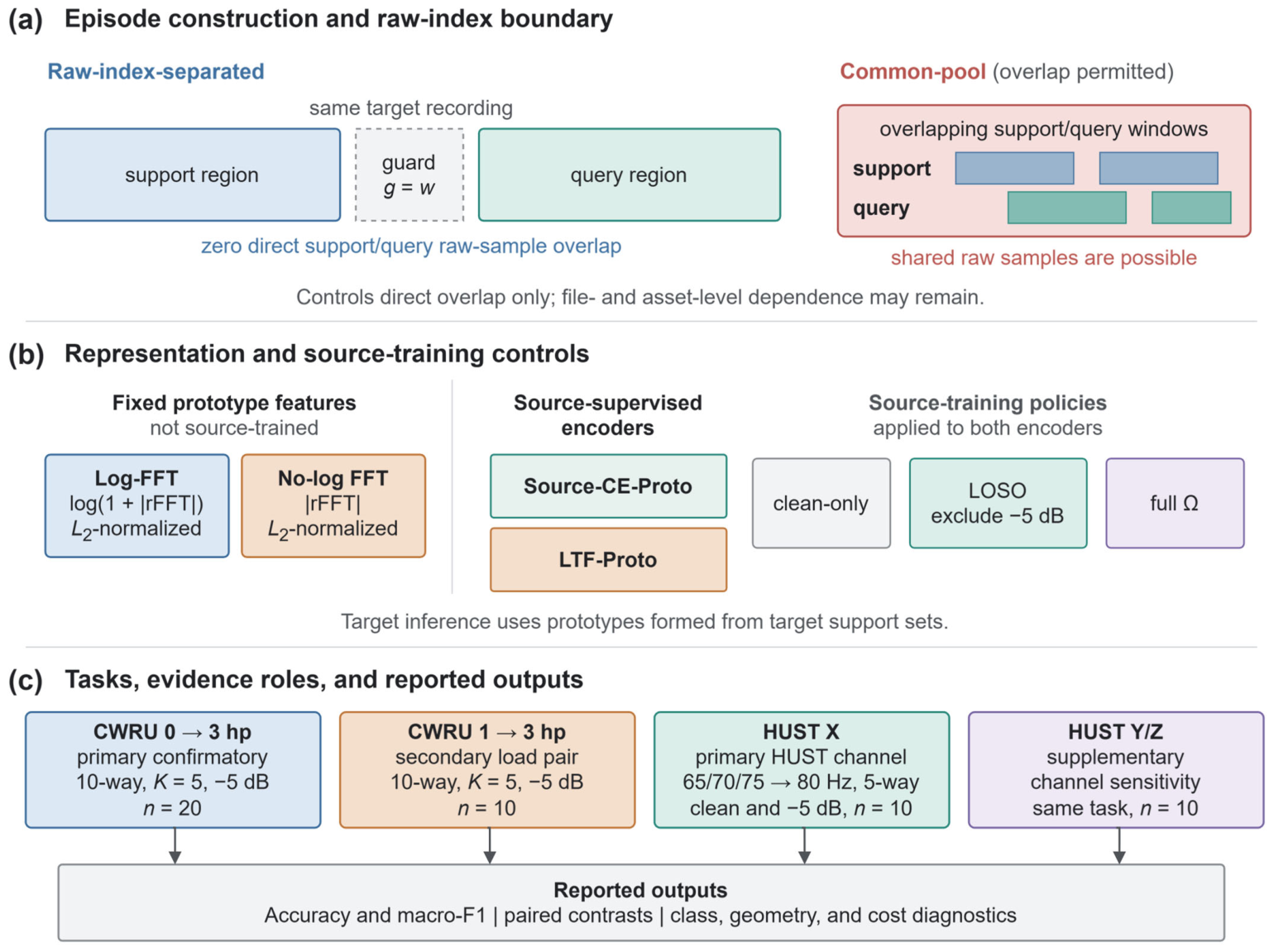
Figure 1 separates the evaluation-side raw-index audit from the source-training and feature-construction controls. The term “raw-index-separated” denotes only the absence of direct raw-sample overlap under the declared window geometry. Support and query windows still originate from different regions of the same target recording and are not assumed to be statistically independent. Panel (c) maps the primary, secondary, and supplementary tasks to the reported metric and diagnostic outputs.

Table 1. Experiment matrix and evidence roles.

Task	Source to Target	Classes	Target Condition	K	Seeds	Evidence Role
CWRU primary	0 hp to 3 hp	10	−5 dB	5	20	confirmatory
CWRU additional	1 hp to 3 hp	10	−5 dB	5	10	secondary replication
HUSTbearing primary channel	65/70/75 Hz to 80 Hz, X	5	clean and −5 dB	5	10	second-dataset boundary/sensitivity
HUSTbearing supplementary channels	65/70/75 Hz to 80 Hz, Y/Z	5	clean and −5 dB	5	10	channel sensitivity

Note: K is the number of support examples per class. HUSTbearing X is the primary HUSTbearing channel; Y and Z are supplementary channel-sensitivity analyses. Experimental seed is the inferential unit.

summarizes the experiment matrix. Experimental seeds, rather than episodes or windows, were the inferential replicates.

3.2. Datasets, Task Definitions, and Provenance

The CWRU analysis used the official 12 kHz drive-end signals [5,29]. The ten classes were normal (N); inner-race faults with diameters of 0.007, 0.014, and 0.021 in (0.178, 0.356, and 0.533 mm, respectively; IR007, IR014, and IR021); ball faults with the same three diameters (BA007, BA014, and BA021); and outer-race faults with the same three diameters at the 6 o’clock position (OR007_6, OR014_6, and OR021_6). The primary source files at 0 hp had IDs 97, 105, 169, 209, 118, 185, 222, 130, 197, and 234 in this class order. The corresponding 3 hp target IDs were 100, 108, 172, 212, 121, 188, 225, 133, 200, and 237. The secondary 1 hp source IDs were 98, 106, 170, 210, 119, 186, 223, 131, 198, and 235. Exact file names, MATLAB variable keys, signal lengths, and hashes are provided in the provenance inventory in Supplementary File S1.

HUSTbearing was reconstructed from the official raw ‘.xls’ files because those files preserve speed, vibration-channel identity, file identity, and raw start/end indices required by the audit [9,10]. The verified raw-column order was Time, Speed/Tacho, X, Y, and Z. The Speed/Tacho column was excluded from all vibration inputs. The sampling rate was 25.6 kHz. The five classes were healthy (H), inner-race fault (I), outer-race fault (O), ball fault (B), and combination fault (C). The primary cross-speed task used 65, 70, and 75 Hz source files and 80 Hz target files. X was specified a priori as the primary vibration channel. Y and Z were evaluated only as supplementary sensitivity channels, irrespective of their observed performance. All HUSTbearing results reported in this study were generated from the verified parser and the stated X/Y/Z channel mapping.

Each episode contained N classes. For CWRU, N = 10, with K = 5 support windows and Q = 15 query windows per class; the exploratory geometry program also evaluated K∈{1,5,10}. For HUSTbearing, N = 5, K = 5, and Q = 15. Each seed contained 200 Monte Carlo episodes. Target support labels were used only to form class prototypes. Target query labels were accessed only after prediction for metric calculation; query features, labels, and statistics were not used for source training, normalization fitting, prototype construction, checkpoint selection, or hyperparameter selection.

3.3. Windowing, AWGN, and Per-Window Normalization

Let $x^{(d,c)}={\left\{x_t\right\}}_{t=0}^{L_{d,c}-1}$ denote a raw vibration signal of length $L_{d,c}$ recorded in operating domain d and class c. The start index of a window of length w with stride r is defined in Equation (1):

$$s_n=nr,\hspace{1em}n=0,1,\dots ,⌊{\displaystyle \frac{L_{d,c}-\omega }{r}}⌋$$

(1)

The corresponding window vector is given by Equation (2):

$${\mathit{x}}_{s_n}^{(d,c)}={\left[x_{s_n},x_{s_n+1},\dots ,x_{s_n+w-1}\right]}^{\mathrm{T}}$$

(2)

CWRU used w = 2048 samples and r = 512 samples; HUSTbearing used w = 3200 and r = 800. Each extracted window was normalized independently according to Equation (3):

$$\tilde{x}={\displaystyle \frac{\mathit{x}-\mu (\mathit{x})}{\max \{\sigma (\mathit{x}),\epsilon \}}},\hspace{1em}\hspace{1em}\epsilon ={10}^{-8}$$

(3)

where $\mu (\mathit{x})$ and $\sigma (\mathit{x})$ are the sample mean and standard deviation within that window. No statistic was estimated from a union of target support and query windows.

Additive white Gaussian noise (AWGN) was used as a controlled synthetic stressor. Equation (4) defines its application to the raw signal vector $\mathit{x}$:

$${\mathit{x}}^{\prime }=\mathit{x}+\mathit{\eta },\hspace{1em}\hspace{1em}{\eta }_t~\mathcal{N}(0,{\sigma }_{\eta }^2)$$

(4)

The noise variance in Equation (4) was set from the requested SNR using Equation (5):

$${\sigma }_{\eta }^2={\displaystyle \frac{P_x}{{10}^{{\mathrm{SNR}}_{\mathrm{dB}}/10}}},\hspace{1em}\hspace{1em}{P}_x={\displaystyle \frac{1}{L}}{\displaystyle \sum _{t=0}^{L-1}{x}_t^2}$$

(5)

Here, L is the number of samples in x, ${\eta }_t$ is the $t$th noise sample, $P_x$ is the mean signal power, and ${\mathrm{SNR}}_{\mathrm{dB}}$ is the requested SNR in decibels. For target evaluation, one seed-specific AWGN realization was added to each complete raw target signal before region definition and window extraction. The resulting noisy target signal was shared by all methods and source policies within that seed. Consequently, overlapping target windows inherited samples from the same signal-level noise realization. Different experimental seeds used different target-noise realizations.

For source training, raw windows were first selected by a seed-specific source subsample. On every access, an SNR state was selected from the declared source policy, AWGN was added to the raw source window when applicable, and Equation (3) was then applied once. The source-noise state and waveform were deterministic functions of the experimental seed, epoch, window index, and SNR. Thus, source noise varied reproducibly across epochs and window accesses. The source and target paths shared the order of noise before the final z-score, but they were not identical: source noise was generated per accessed training window, whereas target noise was generated over the complete raw recording before extraction. Thus, the two pipelines used the same preprocessing order but differed in the granularity at which AWGN was generated.

3.4. Raw-Index-Separated and Common-Pool Episodes

For a target signal of length L, let $m=⌊L/2⌋$ and let the guard gap be g. For a half-open raw interval $[a,b)$, Equation (6) defines the admissible window starts:

$$\mathcal{W}(a,b)=\{a+nr:n=0,1,\dots ,⌊(b-a-w)/r⌋\}$$

(6)

Under forward separation, Equation (7) defines the support and query start pools for class c:

$${\mathcal{A}}_c^{\sup }=\mathcal{W}\left(0,m-⌊g/2⌋\right),\hspace{1em}\hspace{1em}{\mathcal{A}}_c^{\mathrm{qry}}=\mathcal{W}\left(m+⌊g/2⌋,L\right)$$

(7)

The primary setting used g = w. Because every window was wholly contained in its assigned region, support and query windows could not share raw indices. This is a sufficient direct-overlap exclusion rule for the evaluated geometry, not a universal independence threshold. Reverse separation swapped the actual front and back candidate pools. Guard-gap sensitivity used $g\in \{w,2w,4w\}$ while preserving feasible support and query pool sizes.

Within these pools, Equation (8) defines the support and query sets sampled without replacement for episode e:

$${\mathcal{S}}_e={\displaystyle \underset{c\in \mathcal{C}}{\cup }{\mathrm{Sample}}_K}({\mathcal{P}}_c^{\sup }),\hspace{1em}\hspace{1em}{\mathcal{Q}}_e={\displaystyle \underset{c\in \mathcal{C}}{\cup }{\mathrm{Sample}}_Q}({\mathcal{P}}_c^{\mathrm{qry}})$$

(8)

where $\mathcal{C}$ is the class set and ${\mathcal{P}}_c^{\sup }$ and ${\mathcal{P}}_c^{\mathrm{qry}}$ contain windows indexed by Equation (7). The comparison condition, termed common-pool construction, sampled $K+Q$ distinct window objects from all sliding windows of the same target class, assigning K to support and Q to query. Although the same object was never selected twice, different objects could overlap in raw samples.

For two windows $a=[s_a,s_a+w)$ and $b=[s_b,s_b+w)$ from the same file and class, Equation (9) defines direct overlap:

$$I_{\mathrm{ov}}(a,b)=\mathbf{1}\{\max (s_a,s_b)<\min (s_a+w,s_b+w)\}$$

(9)

Equation (10) defines an auxiliary near-duplicate indicator that additionally counts adjacent windows whose closest boundaries are no more than one stride apart:

$$I_{\mathrm{near}}(a,b)=\mathbf{1}\left\{I_{\mathrm{ov}}(a,b)=1\hspace{1em}\mathrm{or}\hspace{1em}\min \left(|s_a-s_b-w|,|s_b-s_a-w|\right)\le r\right\}$$

(10)

Here, $\mathbf{1}\{\cdot \}$ denotes the indicator function, which equals 1 when its enclosed condition is true and 0 otherwise.

The episode hit rate was the proportion of query windows having at least one same-class support window satisfying Equation (10). Exact starts, ends, file IDs, overlap counts, and hit rates were retained for every episode in Supplementary File S1.

3.5. Prototype Inference and Controlled Representations

All prototype-based methods used the same target-support decision rule. Given representation $f(\cdot )$, Equation (11) defines the prototype for class c:

$${\mathit{p}}_c={\displaystyle \frac{1}{K}}{\displaystyle \sum _{({\mathit{x}}_i,y_i)\in {\mathcal{S}}_e}\mathbf{1}}\{y_i=c\}f({\mathit{x}}_i)$$

(11)

Equation (12) then assigns each query by squared Euclidean distance:

$$\widehat{y}(\mathit{x})=\arg {\min }_{c\in \mathcal{C}}{‖f(\mathit{x})-{\mathit{p}}_c‖}_2^2$$

(12)

Equation (13) defines the initial fixed reference, denoted Log-FFT, using a one-sided real-input fast Fourier transform (rFFT):

$$f_{\mathrm{LogFFT}}(\tilde{\mathit{x}})={\displaystyle \frac{\log \left(1+|\mathrm{rFFT}(\tilde{\mathit{x}})|\right)}{{‖\log \left(1+|\mathrm{rFFT}(\tilde{\mathit{x}})|\right)‖}_2+\epsilon }}$$

(13)

Equation (14) defines the stronger No-log FFT control, which omitted log compression but retained $L_2$ normalization:

$$f_{\mathrm{NoLogFFT}}(\tilde{\mathit{x}})={\displaystyle \frac{|\mathrm{rFFT}(\tilde{\mathit{x}})|}{{‖|\mathrm{rFFT}(\tilde{\mathit{x}})|‖}_2+\epsilon }}$$

(14)

Additional fixed-feature ablations removed the direct-current (DC) bin from Equation (13), removed $L_2$ normalization, or used the normalized raw time window directly as the prototype feature.

Source-CE-Proto used a source-supervised one-dimensional convolutional encoder followed by target prototype inference. It was not episodically meta-trained and should not be interpreted as a Snell-style Prototypical Network [1]. The CWRU encoder comprised three convolutional stages: $1\to 32$ channels with kernel 64, stride 8, and padding 28; $32\to 64$ with kernel 5 and padding 2; and $64\to 128$ with kernel 3 and padding 1. Each stage used BatchNorm, rectified linear unit (ReLU) activation, and, after the first two stages, max pooling by 2. Adaptive average pooling and a linear $128\to 64$ projection produced an $L_2$-normalized embedding. The GroupNorm control replaced each BatchNorm layer with eight-group GroupNorm while retaining channel dimensions and all other settings. BatchNorm running statistics were learned only from source training and frozen during target support/query evaluation.

The learned time-frequency prototype encoder (LTF-Proto) combined the same time-domain encoder with a learned frequency branch. The log-rFFT magnitude was mapped from $w/2+1$ bins to 96 hidden units and then to 64 dimensions, with ReLU and dropout probability 0.05. The separately normalized time and frequency embeddings were concatenated and passed through a $128\to 64\to 64$ fusion multilayer perceptron before final $L_2$ normalization. Like Source-CE-Proto, LTF-Proto was trained by source-domain cross-entropy rather than episodic meta-learning.

For each learned method, a temporary source classification head W was optimized using the mini-batch cross-entropy loss in Equation (15):

$${\mathcal{L}}_{\mathrm{src}}(\theta ,W)=-{\displaystyle \frac{1}{B}}{\displaystyle \sum _{i=1}^B\log }{\displaystyle \frac{\exp \left({[W{f}_{\theta }({\mathit{x}}_i)]}_{y_i}\right)}{{\displaystyle \sum _{c\in \mathcal{C}}\exp }\left({[W{f}_{\theta }({\mathit{x}}_i)]}_c\right)}}$$

(15)

where B is the mini-batch size, $\theta$ denotes encoder parameters, and ${[W{f}_{\theta }({\mathit{x}}_i)]}_c$ is the source-class logit. The head was discarded before target prototype evaluation.

The HUSTbearing learned encoders used a dataset-specific lightweight architecture: $1\to 16$, $16\to 32$, and $32\to 64$ convolutional blocks with kernels 7, 5, and 3; strides 2, 2, and 1; BatchNorm, ReLU, and max pooling by 2 in each block; adaptive average pooling; and a $64\to 64\to 64$ projection. The HUSTbearing LTF branch followed the same 96-unit frequency and 64-dimensional fusion design described above.

3.6. Source-Training Policies and Experimental Controls

The clean policy added no source noise. Equation (16) defines the full policy, from which an SNR state was selected uniformly at random and independently for each source-window access:

$${\Omega }_{\mathrm{full}}=\{\mathrm{clean},10,5,0,-5,-10 \mathrm{dB}\}$$

(16)

Equation (17) defines the leave-one-SNR-out policy by excluding the evaluated target SNR:

$${\Omega }_{\mathrm{LOSO}}=\{\mathrm{clean},10,5,0,-10 \mathrm{dB}\}$$

(17)

Comparing LOSO with clean training tested whether recovery persisted without direct source exposure to −5 dB. The full-versus-LOSO comparison is a policy contrast: removing −5 dB also changes the relative sampling weights of the remaining source states. It therefore does not isolate a causal effect of exact target-SNR exposure. Neither policy was interpreted as proof of robustness to unseen or real industrial noise.

CWRU source training used at most 220 raw windows per class, 12 epochs, batch size 64, AdamW with learning rate ${10}^{-3}$, and weight decay ${10}^{-4}$. HUSTbearing used at most 80 source windows per class per source speed, 15 epochs, batch size 64, and the same optimizer settings. All learned-model checkpoints corresponded to the final fixed training epoch; no validation-based early stopping or target-based checkpoint selection was used. Experimental seed controlled source-window subsampling, network initialization, data-loader order, source-noise choices and realizations, target AWGN, and episode sampling. Within a seed, target signals and episode references were shared across methods and source policies wherever their protocol roles permitted pairing. For the HUSTbearing learned encoders, the source-window subsampling seed included the vibration channel, so X, Y, and Z used channel-specific pseudorandom source-window subsets under the same per-class and per-speed budget. Learned-model differences across channels were therefore treated as supplementary sensitivity rather than isolated causal effects of channel choice.

The primary CWRU matrix crossed raw-index-separated/common-pool evaluation with Log-FFT, Source-CE-Proto, and LTF-Proto; learned methods were crossed with clean, full, and LOSO source policies. Additional controls comprised: (i) GroupNorm versus BatchNorm for Source-CE-Proto; (ii) forward g = w, 2w, and 4w and reverse g = w target regions; (iii) target SNRs clean, 10, 5, 0, −5, and −10 dB at K = 5; and (iv) K = 1, 5, and 10 at −5 dB. Further analyses covered fixed-feature ablations, the CWRU 1 hp to 3 hp task, and HUSTbearing positive-control and cross-speed results on X, Y, and Z.

The HUSTbearing 80 Hz positive control used disjoint training, support, and query regions. Boundaries were $b_1=⌊0.4L⌋$ and $b_2=⌊0.6L⌋$, with a 3200-sample guard centered at each boundary. This control assessed clean separability under the verified parser, channel mapping, and labels.

3.7. Performance, Overlap, and Statistical Analysis

For episode e with query set ${\mathcal{Q}}_e$, Equation (18) defines accuracy:

$${\mathrm{Acc}}_e={\displaystyle \frac{1}{\left|{\mathcal{Q}}_e\right|}}{\displaystyle \sum _{({\mathit{x}}_i,y_i)\in {\mathcal{Q}}_e}\mathbf{1}}\{\widehat{y}({\mathit{x}}_i)=y_i\}$$

(18)

Macro-F1 was computed across the N episode classes as a secondary metric. Equation (19) defines the seed-level average of the episode accuracies for experimental seed j:

$${\overline{a}}_j={\displaystyle \frac{1}{E}}{\displaystyle \sum _{e=1}^E{\mathrm{Acc}}_{e,j}},\hspace{1em}\hspace{1em}E=200$$

(19)

For paired conditions A and B, the seed-level difference was ${\Delta }_j={\overline{a}}_j^A-{\overline{a}}_j^B$, expressed in percentage points (pp). Equation (20) gives the mean effect and its two-sided 95% paired t interval:

$$\overline{\Delta }={\displaystyle \frac{1}{n}}{\displaystyle \sum _{j=1}^n{\Delta }_j},\hspace{1em}\hspace{1em}\overline{\Delta }\pm t_{0.975,n-1}{\displaystyle \frac{s_{\Delta }}{\sqrt{n}}}$$

(20)

where n is the number of experimental seeds and $s_{\Delta }$ is the sample standard deviation of the paired differences. The paired standardized effect was $d_z=\overline{\Delta }/s_{\Delta }$ when $s_{\Delta }>0$.

Equation (21) defines the primary two-sided p value obtained by exact paired sign-flip enumeration:

$$p_{\mathrm{exact}}=2^{-n}{\displaystyle \sum _{\mathit{s}\in {\{-1,+1\}}^n}\mathbf{1}}\left\{\left|{\displaystyle \frac{1}{n}}{\displaystyle \sum _{j=1}^n{s}_j}{\Delta }_j\right|\ge |\overline{\Delta }|\right\}$$

(21)

In Equation (21), $s_j\in \{-1,+1\}$ is the enumerated sign assigned to the jth paired difference. The enumeration uses a sign-symmetry/exchangeability assumption for the paired differences under the null; “enumerated” describes the computation and does not remove that statistical assumption. Holm adjustment was applied within each declared multi-contrast family. Paired t tests were retained as sensitivity analyses, not as the primary p values. The t-based confidence intervals are reported as paired uncertainty summaries and are not inversions of the enumerated sign-flip tests. C1 belonged to the seven predeclared overlap contrasts, whereas C2–C4 formed the predeclared ordering-and-source-policy family; Holm correction was applied within each family. The corresponding results are reported in Section 4.1. Other representation-specific leakage contrasts, difference-in-differences, SNR/K, temporal, normalization, ablation, secondary-load, and HUSTbearing comparisons were secondary or exploratory as declared before their execution.

3.8. Diagnostic and Computational Analyses

Diagnostic analyses were prespecified before their outputs were generated and were conducted only after the primary evaluation. Seed-aggregated confusion matrices and per-class accuracies were computed from frozen query predictions. For each seed and representation, 50 source windows and 50 target-query windows per class were selected by deterministic seed-specific sampling. Target silhouette coefficients were computed using Euclidean distances. The between/within-class scatter ratio was defined as the class-weighted between-class sum of squares divided by the within-class sum of squares. Source and target centroids were matched by class label, and their mean Euclidean distance was normalized by the square root of the sum of the source and target within-class mean squared radii. Two-dimensional PCA pooled the source and target embeddings for the fixed seed-0 visualization only. These diagnostics were descriptive and were not used to select methods, channels, classes, or experimental conditions.

Temporal stationarity was assessed descriptively using clean CWRU 3 hp recordings and HUSTbearing 80 Hz X-channel recordings. Non-overlapping windows were extracted from the front and back regions defined using g = w. Root-mean-square amplitude, Pearson kurtosis, spectral centroid, power ratios below 0.1 times the Nyquist frequency, from 0.1 to 0.3 times the Nyquist frequency, and above 0.3 times the Nyquist frequency, and normalized autocorrelation at a lag corresponding to one shaft revolution were computed for each window. Region-level means were first computed within each class, after which back-minus-front differences were summarized across classes.

Training wall time, parameter count, peak allocated GPU memory, embedding time per window, and end-to-end episode time were recorded. Experiments were implemented in Python 3.10.20 with PyTorch 2.11.0, NumPy 2.2.6, pandas 2.3.3, SciPy 1.15.3, and scikit-learn 1.7.2. Learned models were measured on an NVIDIA GeForce RTX 5070 Ti Laptop GPU (NVIDIA Corporation, Santa Clara, CA, USA) using CUDA 12.8. FFT timing used NumPy on the CPU. CPU and GPU times were therefore reported as implementation costs, not as a same-device speed competition. Versioned run directories, source-data tables, episode references, audit scripts, code hashes, and figure/table sources were included in Supplementary File S1.

4. Results

4.1. Primary CWRU Factorial Results

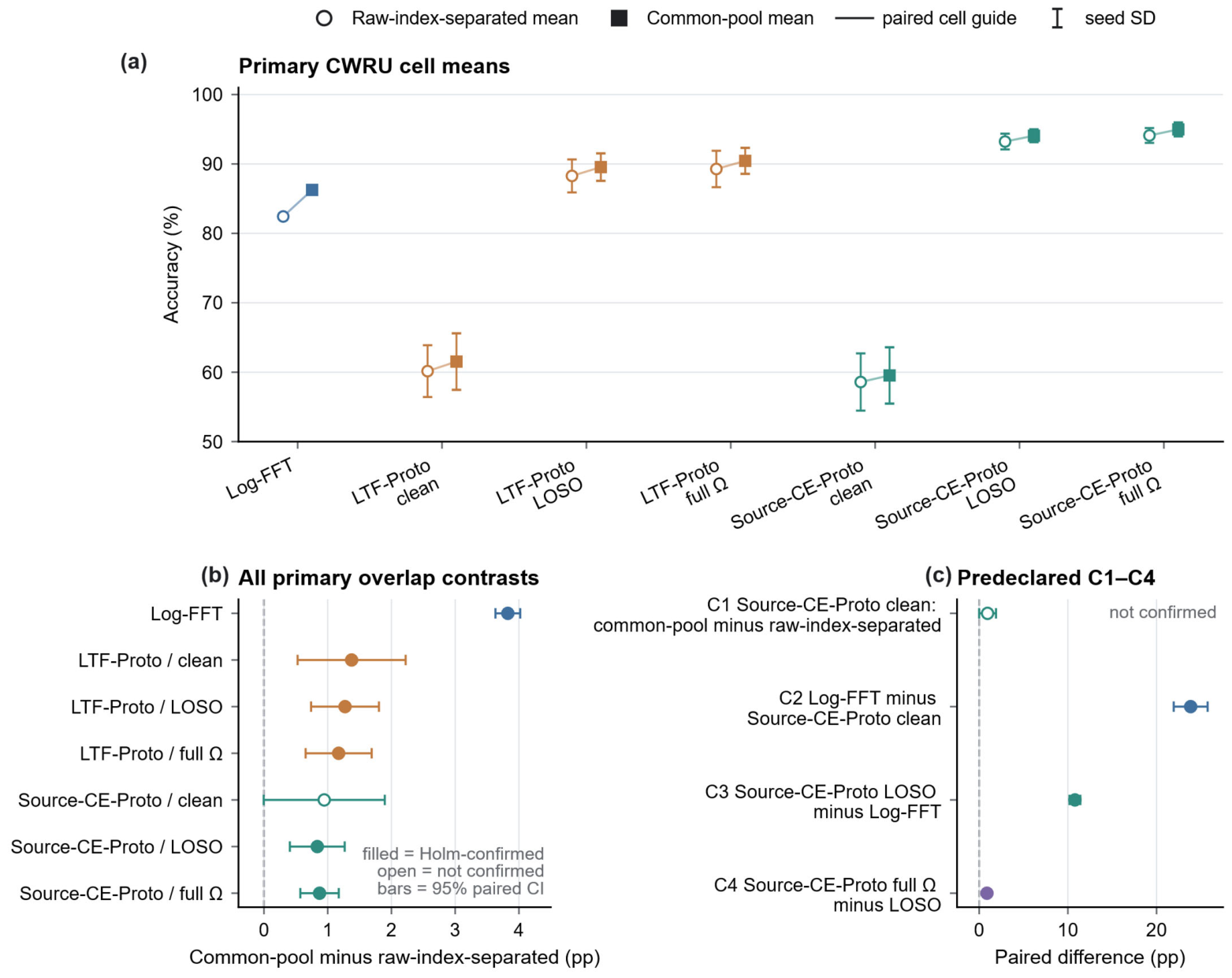
The primary CWRU matrix showed that the measured effect of common-pool episode construction depended on the representation and source policy (

Table 2. Primary CWRU 0 hp to 3 hp results at −5 dB and K = 5.

Representation	Source Policy	n	Separated Accuracy, Mean (SD), %	Common-Pool Accuracy, Mean (SD), %	Separated Macro-F1, Mean (SD), %	Common-Pool Macro-F1, Mean (SD), %	Common-Pool Minus Separated, pp [95% CI]	Exact p	Holm p
Log-FFT	not applicable	20	82.43 (0.44)	86.26 (0.29)	82.11 (0.44)	86.10 (0.30)	+3.83 [+3.63, +4.02]	1.91 × 10−6	1.34 × 10−5
LTF-Proto	clean	20	60.15 (3.73)	61.53 (4.07)	59.63 (3.71)	60.99 (4.15)	+1.38 [+0.53, +2.22]	0.00347	0.00693
LTF-Proto	LOSO (exclude −5 dB)	20	88.27 (2.38)	89.55 (1.98)	87.77 (2.62)	89.23 (2.12)	+1.27 [+0.74, +1.80]	0.00023	0.00093
LTF-Proto	full Ω	20	89.27 (2.62)	90.45 (1.87)	88.80 (2.96)	90.19 (1.94)	+1.17 [+0.65, +1.69]	8.39 × 10−5	0.00042
Source-CE-Proto	clean	20	58.59 (4.12)	59.53 (4.05)	58.43 (4.11)	59.39 (4.08)	+0.95 [−0.004, +1.90]	0.05084	0.05084
Source-CE-Proto	LOSO (exclude −5 dB)	20	93.23 (1.13)	94.06 (0.92)	93.04 (1.20)	93.91 (0.99)	+0.84 [+0.41, +1.27]	0.00066	0.00197
Source-CE-Proto	full Ω	20	94.10 (1.07)	94.98 (1.00)	93.96 (1.13)	94.86 (1.07)	+0.87 [+0.57, +1.17]	1.53 × 10−5	9.16 × 10−5

Note: The task was 10-way, 5-shot, with 20 seeds and 200 episodes per seed. SD denotes the between-seed standard deviation. Confidence intervals are paired seed-level t intervals. p values are two-sided enumerated paired sign-flip probabilities under the stated sign-symmetry/exchangeability assumption with Holm correction across the seven displayed overlap contrasts. The clean Source-CE-Proto contrast was not confirmed at α = 0.05.

; Figure 2). Log-FFT increased from 82.43% under raw-index-separated evaluation to 86.26% under common-pool evaluation, a paired gap of +3.83 percentage points (pp; 95% CI: [+3.63, +4.02]; Holm-adjusted exact $p=1.34\times {10}^{-5}$). The corresponding gaps were smaller for the six learned cells, ranging from +0.84 to +1.38 pp. Five of those six gaps were confirmed after Holm adjustment. The exception was clean Source-CE-Proto: its +0.95 pp estimate had a 95% CI of [−0.004, +1.90] and exact p = 0.05084. It was therefore not treated as a confirmed overlap effect.

The secondary macro-F1 values closely tracked accuracy because every episode used a balanced query set. The largest accuracy-macro-F1 separation in Table 2 was less than 0.6 pp, and no principal interpretation changed when macro-F1 was examined.

The full crossing also permitted representation-specific difference-in-differences. Relative to the clean Source-CE-Proto overlap gap, the Log-FFT gap was larger by +2.88 pp (95% CI: [+1.99, +3.77]; exact $p=1.14\times {10}^{-5}$). The corresponding differences for the other learned cells ranged from −0.11 to +0.43 pp and were not confirmed. Thus, the primary matrix did not support a single method-independent overlap correction; it showed that overlap sensitivity varied across the tested representation/policy cells.

Under raw-index-separated evaluation, source-noise policy strongly changed the performance of the source-supervised encoder relative to the Log-FFT implementation (

Table 3. Predeclared primary CWRU paired contrasts.

ID	Defined Difference	n	Difference, pp [95% CI]	Exact p	Holm p	Paired dz
C1	Source-CE-Proto clean: common-pool minus raw-index-separated	20	+0.95 [−0.004, +1.90]	0.05084	0.05084	0.47
C2	Log-FFT minus Source-CE-Proto clean under raw-index-separated evaluation	20	+23.85 [+21.94, +25.76]	1.91 × 10−6	5.72 × 10−6	5.85
C3	Source-CE-Proto LOSO minus Log-FFT under raw-index-separated evaluation	20	+10.79 [+10.18, +11.41]	1.91 × 10−6	5.72 × 10−6	8.22
C4	Source-CE-Proto full Ω minus LOSO under raw-index-separated evaluation	20	+0.88 [+0.60, +1.16]	7.63 × 10−6	7.63 × 10−6	1.47

Note: C1 is the clean Source-CE-Proto common-pool-minus-separated contrast. C2–C4 are raw-index-separated contrasts. Differences and 95% CIs are paired at the experimental-seed level; CIs are paired t intervals. p values are two-sided enumerated paired sign-flip probabilities under the stated sign-symmetry/exchangeability assumption, with Holm correction within each predeclared family.

). Log-FFT exceeded clean Source-CE-Proto by +23.85 pp. Source-CE-Proto trained with LOSO, which had never received −5 dB source windows, exceeded Log-FFT by +10.79 pp. The full policy exceeded LOSO by +0.88 pp under this policy contrast; because excluding −5 dB also changes the relative sampling weights of the remaining source states, this difference does not isolate a causal effect of exact target-SNR exposure. The LOSO result shows that direct exposure to the exact target SNR was not necessary for the observed learned-encoder recovery. However, these contrasts describe ordering relative to the specified log-compressed FFT reference and do not establish intrinsic architecture superiority.

4.2. SNR, Shot-Count, and Temporal-Region Sensitivity

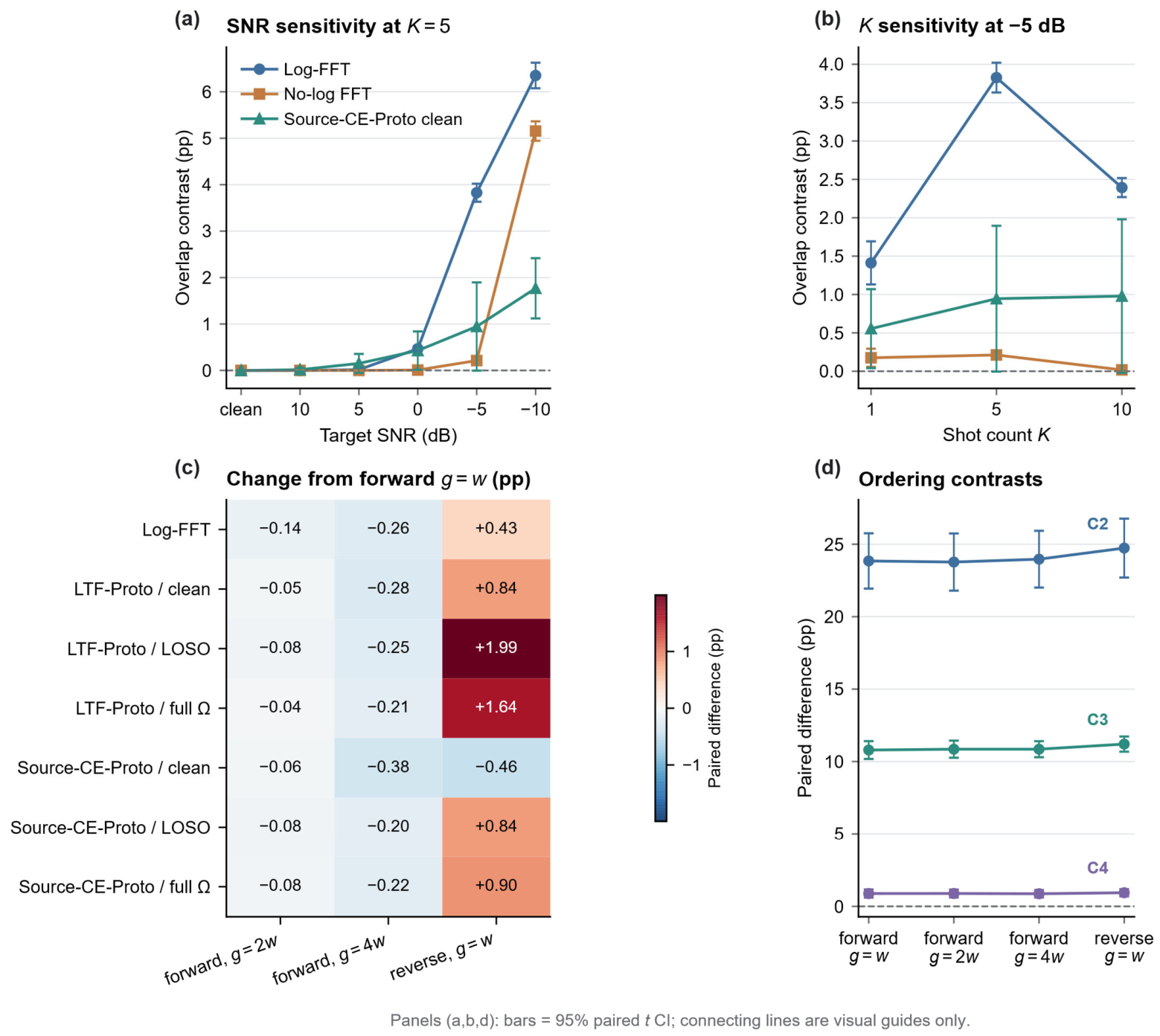
The separate SNR/K program showed that overlap effects were neither uniform across target noise nor monotonic in shot count (Figure 3a,b). At clean and 10 dB targets, all three audited representations had gaps close to zero. At 0 dB, Log-FFT had a +0.47 pp gap, whereas No-log FFT remained near zero (+0.01 pp). At −5 dB, the gaps were +3.83 pp for Log-FFT, +0.21 pp for No-log FFT, and +0.95 pp for clean Source-CE-Proto. At −10 dB, they increased to +6.35, +5.15, and +1.77 pp, respectively. These patterns show that a representation with near-ceiling separated accuracy can have little room for common-pool construction to increase the measured score, whereas the same construction can have a larger effect in a degraded operating regime.

At −5 dB, the Log-FFT gap was +1.41 pp for K = 1, +3.83 pp for K = 5, and +2.39 pp for K = 10. The No-log FFT gaps were +0.18, +0.21, and +0.02 pp, while clean Source-CE-Proto gaps were +0.56, +0.95, and +0.98 pp. Because these sequences were not consistently increasing, the results do not support a universal shot-count law. The −5 dB, K = 5 value in this sensitivity analysis came from a separate run; the primary estimate remains that reported in Section 4.1.

Increasing the forward guard from w to 2w changed absolute accuracy by no more than 0.14 pp in any cell. At 4w, all cells decreased modestly, by 0.21 to 0.38 pp. Reversing the actual support and query regions had larger and method-dependent effects: changes ranged from −0.46 pp for clean Source-CE-Proto to +1.99 pp for LTF-Proto LOSO (Figure 3c). Nevertheless, the predeclared ordering contrasts remained similar across all four geometries. Log-FFT minus clean Source-CE-Proto ranged from +23.77 to +24.73 pp; Source-CE-Proto LOSO minus Log-FFT ranged from +10.79 to +11.20 pp; and full minus LOSO ranged from +0.86 to +0.93 pp (Figure 3d).

Front/back stationarity summaries provided a complementary check. Across the ten CWRU classes, mean back-minus-front differences were small for root-mean-square amplitude (RMS) (+0.0022), spectral centroid (−8.5 Hz), band-energy ratios (absolute mean differences below 0.005), and one-revolution autocorrelation (−0.0003), with class-level intervals spanning zero. Some individual classes nevertheless showed larger temporal changes. Together with the reverse-split results, this indicates that the primary contrasts were not created solely by the forward midpoint assignment, but same-recording temporal-region dependence was not absent.

4.3. Normalization, Fixed-Feature Construction, and Diagnostics

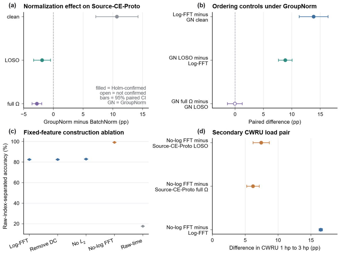
The GroupNorm control showed that replacing BatchNorm with a normalization family that does not use batch running moments altered the magnitude of the clean/noisy discrepancy but did not fully explain the ordering relative to Log-FFT (

Table 4. Normalization, fixed-feature, and secondary-load controls.

Control	ID	Defined Difference	n	Difference, pp [95% CI]	Exact p	Holm p
GroupNorm control	N1	GroupNorm minus BatchNorm under clean training	10	+10.69 [+7.13, +14.24]	0.00195	0.00586
GroupNorm control	N4	Log-FFT minus GroupNorm under clean training	10	+13.84 [+11.30, +16.39]	0.00195	0.00586
GroupNorm control	N5	GroupNorm LOSO minus Log-FFT	10	+8.85 [+7.65, +10.05]	0.00195	0.00586
GroupNorm control	N6	GroupNorm full Ω minus GroupNorm LOSO	10	−0.04 [−1.34, +1.27]	0.95898	0.95898
FFT ablation	no_log	No-log FFT minus Log-FFT	20	+16.66 [+16.48, +16.84]	1.91 × 10−6	7.63 × 10−6
FFT ablation	no_l2	No-L2 FFT minus Log-FFT	20	+0.42 [+0.38, +0.46]	1.91 × 10−6	7.63 × 10−6
FFT ablation	no_dc	Remove-DC FFT minus Log-FFT	20	0.00 [0.00, 0.00]	1	1
FFT ablation	raw_time	Raw-time prototype minus Log-FFT	20	−64.80 [−64.98, −64.61]	1.91 × 10−6	7.63 × 10−6
Additional CWRU pair	A5	No-log FFT minus Source-CE-Proto LOSO	10	+7.43 [+6.19, +8.67]	0.00195	0.01367
Additional CWRU pair	A6	No-log FFT minus Source-CE-Proto full Ω	10	+6.18 [+5.23, +7.14]	0.00195	0.01367
Additional CWRU pair	A7	No-log FFT minus Log-FFT	10	+16.50 [+16.24, +16.75]	0.00195	0.01367

Note: GroupNorm and additional-pair contrasts use 10 seeds; FFT ablations use 20 seeds. Differences and 95% CIs are computed across experimental seeds; CIs are seed-level t intervals. p values are two-sided enumerated paired sign-flip probabilities under the stated sign-symmetry/exchangeability assumption, with Holm adjustment within the corresponding declared family. The zero remove-DC contrast has zero paired variance and therefore no defined paired t statistic; its enumerated sign-flip and Holm p values are both 1.

; Figure 4a,b). This replacement also affects optimization dynamics and learned representations, so the result does not uniquely isolate BatchNorm running-statistic mismatch. Replacing BatchNorm with GroupNorm increased clean Source-CE-Proto accuracy by +10.69 pp. In contrast, GroupNorm reduced LOSO and full-policy accuracy by −1.90 and −2.77 pp, respectively. Under GroupNorm, Log-FFT still exceeded the clean encoder by +13.84 pp, while GroupNorm LOSO still exceeded Log-FFT by +8.85 pp. The full-minus-LOSO contrast under GroupNorm was −0.04 pp (95% CI: [−1.34, +1.27]) and was not confirmed. The full-versus-LOSO policy contrast was therefore small under GroupNorm.

The fixed-feature ablation materially changed the scientific interpretation (Table 4; Figure 4c). Removing log compression increased separated accuracy from 82.43% to 99.09%, a paired gain of +16.66 pp. Removing $L_2$ normalization from the log feature produced only +0.42 pp. Removing the DC bin had exactly zero effect, consistent with prior per-window mean removal. Raw-time prototypes achieved 17.64%, or −64.80 pp relative to Log-FFT. Thus, frequency-domain structure was important in the tested CWRU task, but the hypothesis that log compression drove FFT performance was not supported by the direct ablation.

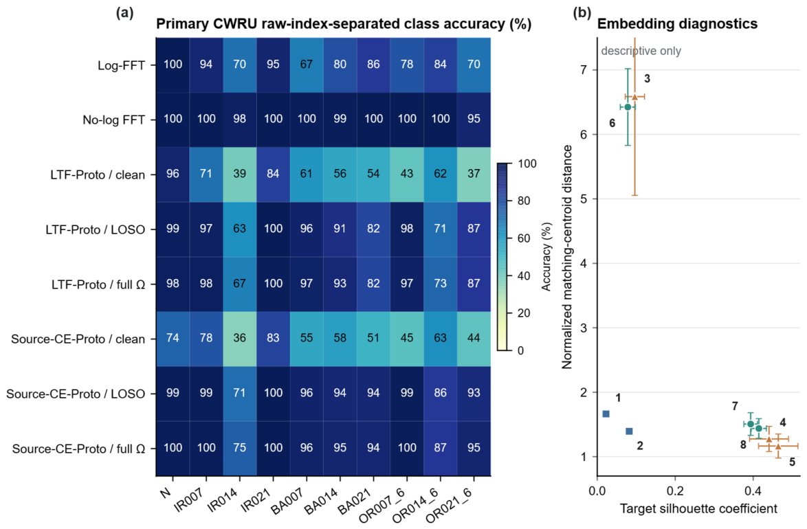
Classwise and embedding analyses further cautioned against a single-mechanism explanation (Figure 5). No-log FFT achieved class accuracies from 95.00% to 100.00%; its weakest class was OR021_6. Log-FFT ranged from 67.39% to 99.97%, and clean Source-CE-Proto ranged from 35.76% to 82.91%. Noise-trained learned encoders improved most classes but remained heterogeneous. Relative to Log-FFT, removing log compression increased the target silhouette coefficient from 0.022 to 0.082 and the between/within-class scatter ratio from 0.087 to 0.268, while decreasing the normalized source-target matching-centroid distance from 1.663 to 1.394. At the same time, global embedding geometry did not rank representations in the same order as accuracy: full-policy Source-CE-Proto and LTF-Proto had higher target silhouette coefficients of 0.414 and 0.464 despite lower accuracies of 94.10% and 89.27%. No single geometry statistic uniquely accounted for episodic performance.

4.4. Secondary CWRU Load Pair

The predeclared CWRU 1 hp to 3 hp task reproduced the fixed-feature sensitivity observed in the primary load pair. Under raw-index-separated −5 dB evaluation, No-log FFT achieved 99.10%, compared with 82.60% for Log-FFT, 91.67% for Source-CE-Proto LOSO, and 92.91% for Source-CE-Proto full Ω (

Table 5. Cross-task raw-index-separated accuracy summary at −5 dB.

Dataset/Task	Channel	Target	Representation	Source Policy	n	Accuracy, Mean (SD), %	95% CI, %
CWRU 0 hp to 3 hp	DE	−5 dB	No-log FFT	not applicable	20	99.09 (0.15)	[99.02, 99.16]
CWRU 0 hp to 3 hp	DE	−5 dB	Log-FFT	not applicable	20	82.43 (0.44)	[82.23, 82.64]
CWRU 0 hp to 3 hp	DE	−5 dB	Source-CE-Proto	full Ω	20	94.10 (1.07)	[93.60, 94.60]
CWRU 0 hp to 3 hp	DE	−5 dB	Source-CE-Proto	LOSO (exclude −5 dB)	20	93.23 (1.13)	[92.70, 93.76]
CWRU 1 hp to 3 hp	DE	−5 dB	No-log FFT	not applicable	10	99.10 (0.17)	[98.98, 99.22]
CWRU 1 hp to 3 hp	DE	−5 dB	Log-FFT	not applicable	10	82.60 (0.39)	[82.32, 82.89]
CWRU 1 hp to 3 hp	DE	−5 dB	Source-CE-Proto	full Ω	10	92.91 (1.27)	[92.00, 93.82]
CWRU 1 hp to 3 hp	DE	−5 dB	Source-CE-Proto	LOSO (exclude −5 dB)	10	91.67 (1.65)	[90.49, 92.85]
HUSTbearing 65/70/75 Hz to 80 Hz	X	−5 dB	Log-FFT	not applicable	10	59.98 (0.65)	[59.51, 60.44]
HUSTbearing 65/70/75 Hz to 80 Hz	X	−5 dB	No-log FFT	not applicable	10	86.21 (1.16)	[85.38, 87.04]
HUSTbearing 65/70/75 Hz to 80 Hz	X	−5 dB	Source-CE-Proto	LOSO (exclude −5 dB)	10	65.41 (3.53)	[62.89, 67.94]
HUSTbearing 65/70/75 Hz to 80 Hz	X	−5 dB	Source-CE-Proto	full Ω	10	65.47 (5.41)	[61.60, 69.34]
HUSTbearing 65/70/75 Hz to 80 Hz	Y	−5 dB	Log-FFT	not applicable	10	63.85 (1.07)	[63.08, 64.61]
HUSTbearing 65/70/75 Hz to 80 Hz	Y	−5 dB	No-log FFT	not applicable	10	99.27 (0.14)	[99.17, 99.38]
HUSTbearing 65/70/75 Hz to 80 Hz	Y	−5 dB	Source-CE-Proto	LOSO (exclude −5 dB)	10	72.36 (4.19)	[69.36, 75.36]
HUSTbearing 65/70/75 Hz to 80 Hz	Y	−5 dB	Source-CE-Proto	full Ω	10	73.28 (4.09)	[70.36, 76.21]
HUSTbearing 65/70/75 Hz to 80 Hz	Z	−5 dB	Log-FFT	not applicable	10	56.47 (0.74)	[55.94, 57.00]
HUSTbearing 65/70/75 Hz to 80 Hz	Z	−5 dB	No-log FFT	not applicable	10	90.39 (0.57)	[89.99, 90.80]
HUSTbearing 65/70/75 Hz to 80 Hz	Z	−5 dB	Source-CE-Proto	LOSO (exclude −5 dB)	10	58.43 (4.78)	[55.01, 61.85]
HUSTbearing 65/70/75 Hz to 80 Hz	Z	−5 dB	Source-CE-Proto	full Ω	10	59.81 (4.52)	[56.58, 63.05]

Note: DE denotes the drive-end channel used for CWRU. HUSTbearing X is primary, and HUSTbearing Y/Z are supplementary channel-sensitivity analyses. For the learned HUSTbearing encoders, source-window subsampling used channel-specific pseudorandom subsets under the same budget. Values are seed-level means with between-seed SDs; 95% CIs are one-sample t intervals across experimental seeds. These summaries are descriptive under raw-index-separated evaluation and do not establish a causal channel effect, channel superiority, sensor fusion, or generalization to industrial settings.

). No-log FFT exceeded LOSO and full Source-CE-Proto by +7.43 and +6.18 pp and exceeded Log-FFT by +16.50 pp (Table 4; Figure 4d). This second CWRU pair supports the conclusion that fixed-feature construction can change the apparent learned-versus-fixed ordering. It does not establish a universal FFT advantage beyond the two tested CWRU load pairs.

4.5. HUSTbearing Cross-Speed Results

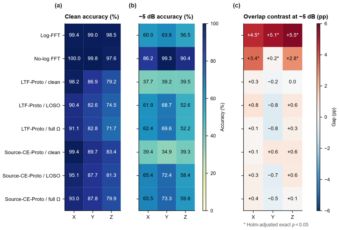
The disjoint-region HUSTbearing 80 Hz positive control produced mean clean accuracies from 97.43% to 100.00% across X/Y/Z and the tested method families, providing a validity check for the parser, class mapping, and separability of the vibration-channel inputs. Clean cross-speed evaluation also remained high for the fixed FFT variants. For Source-CE-Proto, source-noise training often reduced clean-target performance: on X, clean, LOSO, and full policies achieved 99.36%, 95.12%, and 93.01%; on Z, the corresponding values were 83.43%, 81.27%, and 79.95%. Source-noise exposure was therefore not uniformly beneficial outside the noisy target condition.

At −5 dB, HUSTbearing results varied by channel and feature construction (Table 5; Figure 6). On the predeclared X channel, Log-FFT achieved 59.98%, No-log FFT 86.21%, and Source-CE-Proto LOSO/full 65.41%/65.47%. The corresponding Y accuracies were 63.85%, 99.27%, 72.36%, and 73.28%; Z accuracies were 56.47%, 90.39%, 58.43%, and 59.81%. No-log FFT was therefore strong on all three vibration channels, but the channel-dependent magnitudes were not used to select a preferred channel or to imply sensor fusion.

HUSTbearing overlap effects were also representation- and channel-dependent (Figure 6c). Log-FFT common-pool-minus-separated gaps were +4.53, +5.10, and +5.50 pp on X, Y, and Z and remained confirmed after Holm adjustment. No-log FFT gaps were +3.38 pp on X, +0.17 pp on Y, and +2.78 pp on Z; all three were confirmed after Holm correction, although the Y estimate was only +0.17 pp. Most learned-model gaps were not confirmed after correction and included slightly negative estimates on Y. These results reinforce that overlap effects cannot be assigned a method-independent magnitude.

4.6. Computational Cost

The CWRU Source-CE-Proto classifier contained 46,442 trainable parameters, including its temporary source head; LTF-Proto contained 163,562. Across 20 seeds, mean source-training wall time was 3.58 s for clean Source-CE-Proto and 5.03–5.04 s for its full and LOSO policies. LTF-Proto required 4.31 s for clean training and 5.74–5.84 s for LOSO/full training. Mean peak allocated GPU memory ranged from 42.06 to 46.46 MB.

Measured embedding time per window was 0.0108–0.0124 ms for Source-CE-Proto and 0.0194–0.0203 ms for LTF-Proto on the GPU. CPU NumPy feature extraction required 0.0186 ms per window for Log-FFT and 0.0140 ms for No-log FFT. End-to-end processing of one 200-window CWRU episode required 5.98 ms for No-log FFT, 7.07 ms for Log-FFT, and 7.45–8.48 ms for the learned implementations. These values document the computational environment and model budgets. They are not direct CPU-versus-GPU efficiency comparisons.

5. Discussion

5.1. Fixed-Feature Definition Changes the Central Interpretation

Across the tested controls, the data do not support a general learned-versus-fixed ordering. Relative to Log-FFT, source policy changed the ordering: Log-FFT exceeded clean Source-CE-Proto, whereas LOSO and full-policy Source-CE-Proto exceeded Log-FFT. That contrast remained large and stable across temporal geometries. However, No-log FFT reached 99.09% in the primary CWRU task and 99.10% in the secondary load pair, exceeding both noise-trained Source-CE-Proto variants. Across the HUSTbearing channels, No-log FFT reached 86.21–99.27% at −5 dB. The apparent learned-over-fixed crossover was therefore conditional on the log-compressed fixed reference, not a property of fixed versus learned representations in general.

The fixed-feature ablation identifies feature construction as an additional benchmark variable. The evidence supports a methodological conclusion rather than a method-family conclusion: benchmark interpretation can change with overlap control, source-noise policy, normalization, and the exact definition of a fixed feature. None of these factors should be hidden inside a generic baseline name.

5.2. Raw-Index Separation Controls One Leakage Class, Not All Dependence

The primary Log-FFT gap of +3.83 pp shows that assigning windows from a shared overlapping pool can raise measured performance in the tested noisy CWRU setting. HUSTbearing Log-FFT gaps of approximately +4.5 to +5.5 pp provide a second-dataset example. The primary clean Source-CE-Proto estimate, by contrast, was +0.95 pp and not confirmed. No-log FFT showed a small +0.21 pp CWRU gap at −5 dB and a channel-dependent HUSTbearing pattern. The overlap effect was therefore not a constant property of the episode geometry alone; it depended on the representation, performance regime, and, descriptively for HUSTbearing, vibration channel. This representation-dependent episode-internal effect complements earlier leakage studies focused on segment-wise, bearing-wise, and conventional train/test partitions [5,6,7,8].

The SNR and K analyses reinforce this interpretation. Gaps were negligible near the ceiling, increased under severe degradation for some representations, and were not monotonic in K. A shared-pool episode can expose a query to a near-duplicate support window, but the resulting accuracy change depends on whether that local similarity resolves errors that the representation would otherwise make. Reporting only the fraction of overlapping or near-adjacent windows is therefore insufficient. Geometry and performance effects should be reported together.

Raw-index separation should also not be equated with independence. Support and query windows remain in the same file and can share bearing identity, acquisition chain, periodic structure, and slow temporal characteristics. The reverse split changed some absolute accuracies by up to approximately 2 pp, and g = 4w caused small systematic reductions. Stationarity summaries were broadly similar across front and back regions on average, but individual classes showed temporal variation. The appropriate claim is zero direct raw-sample overlap under the declared geometry, not complete removal of leakage or dependence.

5.3. Source-Noise Policy and Normalization Are Separable Benchmark Factors

LOSO training was a central control because the full source policy included the evaluated target SNR. In the primary CWRU task, LOSO Source-CE-Proto exceeded Log-FFT by +10.79 pp despite never receiving −5 dB source windows. The full policy exceeded LOSO by +0.88 pp under this policy contrast; because excluding −5 dB also changes the relative sampling weights of the remaining source states, this difference does not isolate a causal effect of exact target-SNR exposure. Similar LOSO recovery was observed in the additional CWRU task and in HUSTbearing. Direct matched-SNR exposure was therefore not necessary for the main learned-encoder recovery relative to Log-FFT, although the experiment does not establish generalization to arbitrary unseen noise distributions.

The GroupNorm results show why source policy and normalization must be reported separately. GroupNorm substantially improved the clean encoder but slightly reduced both noise-trained encoders. The clean-versus-noise-trained separation was consequently smaller, yet the ordering relative to Log-FFT remained. The result is consistent with, but does not uniquely isolate, a contribution from BatchNorm running-statistic mismatch because changing the normalization family also affects optimization dynamics and learned representations. The unresolved GroupNorm full-minus-LOSO contrast also cautions against presenting inclusion of the exact target SNR as a universally beneficial augmentation choice.

Source-noise exposure can have adverse effects outside the target stress condition. In clean HUSTbearing cross-speed evaluation, LOSO and full training reduced several learned-model accuracies relative to clean training. A source policy that performs well at one noisy endpoint may therefore trade away clean-condition performance. Benchmark reports should state the augmentation distribution and show the operating conditions over which the claimed benefit is evaluated.

5.4. Fixed-Feature Construction Changes the FFT Mechanism Account

The FFT ablation shows that log compression was not required for the strong fixed-reference performance. Removing log compression produced the largest ablation improvement, whereas removing $L_2$ normalization had a small effect and removing the DC bin had none. Because Equation (3) removes each window mean, the zero DC result is expected. Raw-time prototypes produced low accuracy, showing that the strong fixed result was not a generic consequence of nearest-prototype inference.

The no-log result is consistent with strong deterministic spectral separation in these public tasks, but the present analyses do not prove a unique physical mechanism. The descriptive geometry changes reported in Section 4.3 are consistent with more discriminative target geometry and closer normalized source-target class centroids after removal of log compression, but they do not isolate why the transformation changes the spectral representation or establish a causal noise mechanism. Classwise accuracy was high but not uniform, with OR021_6 remaining the weakest no-log CWRU class. Embedding diagnostics also did not align monotonically with accuracy: noise-trained learned representations had higher silhouette coefficients than No-log FFT but lower episodic accuracy. PCA, silhouette, scatter, and centroid distance are therefore descriptive aids rather than causal explanations.

The LTF-Proto results provide a related negative finding. Adding a learned log-rFFT branch did not match No-log FFT, even under noise-trained source policies. Possible reasons include loss of useful magnitude structure through log compression, the limited source-training budget, and optimization of a fused representation for source classification rather than target episodic discrimination. These explanations remain hypotheses because a complete component-by-component LTF ablation and activation analysis were outside the controlled experiment program. The result also qualifies prior uses of spectral and time-frequency representations in few-shot diagnosis by showing that the exact transform construction must be reported [3,20,21,22,23].

5.5. HUSTbearing Evidence and Channel Sensitivity

The HUSTbearing analysis used the verified official Time, Speed/Tacho, X, Y, Z ordering and independently audited channel provenance. Clean positive controls near 97–100% across channels and method families provide a separability sanity check under the verified parser and label mapping.

The cross-speed task remained sensitive to feature construction and channel. No-log FFT ranged from 86.21% on X to 99.27% on Y at −5 dB, whereas Source-CE-Proto full ranged from 59.81% on Z to 73.28% on Y. Overlap gaps also differed across X/Y/Z. Because X was specified a priori as the primary channel, the Y and Z results are interpreted only as supplementary sensitivity analyses. The channel program supports a bounded statement that measured magnitudes vary across vibration axes; it does not establish channel superiority, sensor fusion, or invariance.

HUSTbearing also does not provide validation in an industrial setting. It uses a different public test rig, speed shift, window length, sampling rate, class taxonomy, and dataset-specific learned encoder. The analysis shows that the same audit questions remain meaningful after dataset and channel provenance are verified, but the numerical effects are task-specific. The need for partition-before-windowing and explicit guard regions is consistent with recent leakage-resistant supervised evaluation on HUSTbearing [28], while the present analysis extends that concern to few-shot support/query construction.

5.6. Implications for Benchmarking and Online Diagnosis

For offline benchmarking, the minimum reproducibility unit should include raw file identity, window start/end indices, support/query role, source policy, target-noise realization, experimental seed, and a precise feature definition. A statement such as “FFT baseline” or “source-noise training” is too coarse when log compression, normalization, source SNR distribution, and target access can change the conclusion. Seed-level values and paired episode references should accompany aggregate tables.

For online systems, the results imply a provenance requirement rather than a validated deployment benefit. Rolling buffers can generate highly overlapping windows, and retrospective evaluation can inadvertently place nearly identical raw samples in labeled reference and evaluation sets. An online study should define how long support/reference windows remain valid, whether evaluation windows can overlap them, how adaptation updates are separated from scoring, and whether temporal drift changes the effective task. The present public-dataset experiments do not determine an optimal buffer, adaptation schedule, or alarm policy.

5.7. Limitations

Several limitations define the evidence ceiling. First, raw-index-separated support and query windows remain from different regions of the same recording. Bearing-level and asset-level independence were not available for the primary tasks, and periodic similarity or acquisition-specific signatures may remain.

Second, target corruption used AWGN. Colored, impulsive, non-Gaussian, nonstationary, and mixed industrial noise were not tested. Within AWGN, the full and LOSO SNR sets and uniform per-access sampling were fixed controls rather than optimized augmentation designs; alternative SNR grids, sampling probabilities, or noise mixtures may change the results. The present evidence describes performance at declared synthetic SNRs, not general noise robustness.

Third, Source-CE-Proto is source-supervised rather than episodically meta-trained. The study does not estimate the performance of the full Prototypical Network family, MAML-family methods, transformer-enhanced prototypes, or self-supervised few-shot models. These recent approaches were positioned in the literature but not added as numerical baselines because their pretraining, target access, episodic objectives, and budgets differ from the controlled audit.

Fourth, the dataset scope comprises two CWRU load pairs and one HUSTbearing speed-shift task. Paderborn, XJTU-SY, IMS, run-to-failure datasets, and industrial plant data were not added. A third dataset would require bearing-level split and protocol-comparability controls before it could support broader generality.

Fifth, the mechanism analyses were post-evaluation and descriptive. Confusion matrices, classwise accuracy, FFT ablations, PCA, silhouette, and centroid distances narrow plausible explanations but do not prove causality. Attribution analyses such as gradient-weighted class activation mapping (Grad-CAM) or Shapley additive explanations (SHAP) were not included; they would require a separate design linking attributions to physically interpretable signal regions.

Sixth, the training budget was deliberately compact and fixed within each dataset. Per-epoch learning curves were not retained in the experiments and were not reconstructed after outcomes were known. Final source metrics, available checkpoint manifests and hashes, source-run provenance, wall times, parameter counts, memory, and inference records are provided instead.

Finally, n = 10 secondary analyses have coarse exact sign-flip resolution, and exploratory families should not be interpreted as confirmatory discoveries. The 20-seed primary task provides stronger paired evidence, but statistical confirmation does not remove the dependence and scope limitations above.

6. Conclusions

This study shows that few-shot bearing-diagnosis benchmark conclusions in the tested public-dataset tasks depend on more than the nominal model name. In the primary CWRU task, common-pool episodes produced a confirmed +3.83 pp gap for Log-FFT, whereas the +0.95 pp gap for clean Source-CE-Proto was not confirmed. LOSO source training substantially improved the learned encoder without direct exposure to the evaluated −5 dB SNR, and the full-versus-LOSO policy contrast was small relative to that recovery. GroupNorm changed effect magnitude without removing source-policy sensitivity relative to Log-FFT. Most importantly, removing log compression raised the fixed FFT reference to 99.09% and changed the learned-versus-fixed interpretation in both tested CWRU load pairs. HUSTbearing analyses likewise showed feature- and channel-dependent magnitudes.

The supported conclusion is methodological rather than a general method ranking. Few-shot bearing benchmarks should report raw support/query provenance, direct-overlap controls, source-noise distributions, normalization behavior, exact feature construction, and seed-level paired results. Raw-index separation guarantees zero direct raw-sample overlap for the declared geometry, but it does not create asset-level independence or establish robustness in industrial settings.