Article

Thermal Diffusivity and Thermal Conductivity of Serpentine Minerals vs. Temperature, Pressure, Structure, and Composition: Implications for Subducting Slabs

by
Anne M. Hofmeister
Department of Earth, Environmental, and Planetary Sciences, Washington University, St. Louis, MO 63130, USA
Minerals 2026, 16(5), 509; https://doi.org/10.3390/min16050509
Submission received: 19 March 2026 / Revised: 18 April 2026 / Accepted: 9 May 2026 / Published: 12 May 2026

Abstract

Heat transport properties of serpentine minerals are important to the thermal state of subduction zones, but available data contain systematic errors from contact losses, radiative gains, deformation with pressure (P), and/or modelling short-comings. Here, laser flash analysis (LFA) provides thermal diffusivity (D) within ±3% as a function of temperature (T) of perpendicularly oriented, nearly pure Mg3Si2O5(OH)4 polymorphs, Al-rich lizardite with minor brucite, three serpentinites, plus chrysotile and lizardite near Ni3Si2O5(OH)4. Visible spectra show that Fe is mostly ferric and Cr3+ occasionally occupies tetrahedral sites. The proposed coupled substitution of Al3+ + OH replacing Si4+ + O2− accounts for extra OH peaks in infrared spectra. Rietveld refinements and infrared spectra reveal that serpentine dehydration in LFA runs begins near 800 K. Thermal conductivity (K) vs. T is calculated within ~±5% from D, available heat capacity data, and ambient density. For antigorite, D and K are strongly anisotropic whereas chrysotile has extreme differences, but lizardite is nearly isotropic. A thermodynamic identity provides ∂(lnK)/∂P = 11 ± 1% Gpa−1 for soft serpentine, double that of hard olivine. Lizardite becomes more thermally conductive than olivine near the 1 bar decomposition temperature, which increases with P. Through feedback, and because released H2O vapor carries heat upwards, P,T conditions in serpentinized slabs follow the decomposition phase boundary during subduction.

1. Introduction

Serpentine minerals are tri-octahedral layer silicates, ideally Mg3Si2O5(OH)4. For a detailed description, see [1,2] and citations therein. In summary:
Chemical substitutions are generally low, although incorporation of Al and Fe is common, occurs in both cation sites, and is sometimes extensive. An exception is Ni replacing Mg almost entirely in certain localities [3].
The structures of serpentines are of great interest, yet crystallographic puzzles remain despite a century of study. Unresolved issues stem from a mismatch existing between their internal layers of silica tetrahedra and Mg-rich octahedra, resulting in curved layers and three distinct structural polytypes. Layers in chrysotile form concentric, long cylinders (tubules) and a fibrous habit, which makes this polytype easily identified [2]. In antigorite, misfit is accommodated by an alternating wave pattern (modulation). The most abundant polytype, lizardite, is very fine-grained which permits flat layers to exist locally. Subtypes exist. Lizardite commonly occurs in the 1T subtype, whereas chrysotile mostly has the 2Mc1 structure. Complexities persist to very fine scales as revealed by TEM studies [2].
Serpentine minerals form mainly during hydrothermal alteration of ultramafic rocks, i.e., dunites, peridotites, or pyroxenites. Hence, serpentinites are important constituents of slabs and hydrated upper mantle. Establishing their physical properties as functions of temperature (T) and pressure (P) is needed to interpret geophysical data on subduction zones, and to understand associated processes. Fluid circulation is of particular interest, given hydration reactions such as the following:
2 Mg 2 SiO 4 ( forsterite ) + 3 H 2 O Mg 3 Si 2 O 5 ( OH ) 4 ( serpentine ) + Mg ( OH ) 2 ( brucite )
and
2 Mg 2 SiO 4 + 2 MgSiO 3 + 4 H 2 O 2 Mg 3 Si 2 O 5 ( OH ) 4 .
Iron in olivine partitions into serpentine but also forms magnetite (Fe3O4). Variable amounts of magnetite in serpentinites have been linked to T of formation and partitioning of Fe into brucite [4].
Knowledge of serpentine heat transport properties (thermal conductivity, K and thermal diffusivity, D) is essential to geophysical studies because K (or D), along with boundary conditions, govern thermal evolution. Fourier’s laws quantify diffusion of heat (see, e.g., [5,6]). In 3-dimensions:
= K T   and   ρ c P T t = · K T .
where ℑ is flux (energy per area per time), ρ is density, cP is specific heat (heat capacity on a per mass basis), and t is time.
  • Equation (3) is based on the absence of deformation and other energy-consuming processes.
  • Although diffusion of heat at low temperature is historically denoted as conduction, Fourier’s equations are macroscopic and so cannot differentiate between possible microscopic mechanisms inside the material (e.g., conduction vs. radiation).
Equation (3) neglects internal heating, as is the case for experiments. Fourier’s original, one-dimensional heat equation pertains to many types of experiments:
T t = D 2 T z 2 .
Comparing Equations (3) and (4) links D and K:
K ≡ ρcPD.
The dynamic properties of K and D are thus linked by well-known static properties.
Studies of heat transport of serpentine minerals are few. The focus has been on K and on antigorite [7,8,9]. Data also exist parallel to chrysotile tubules below 298 K [10], on a rock composed of antigorite, calcite, and magnetite [11], and on lizardite-rich serpentinites [12,13]. However, physical contacts were used, except for [13], and so experimental uncertainties in data from [7,8,9,10,11,12] are large and variable, as follows:
Oxides are electrical insulators which bond poorly with metal thermocouples and heaters. Consequent contact losses reduce K by ~10% per contact and also change with compression [14,15]. In addition to possible deformation upon compression, large crystals are impacted by cracking which adds to contact losses [15], while altering geometry and thickness. Rocks are affected by pores compacting more than mineral grains and by grain rolling.
The temperature dependence of transport properties is affected by several factors:
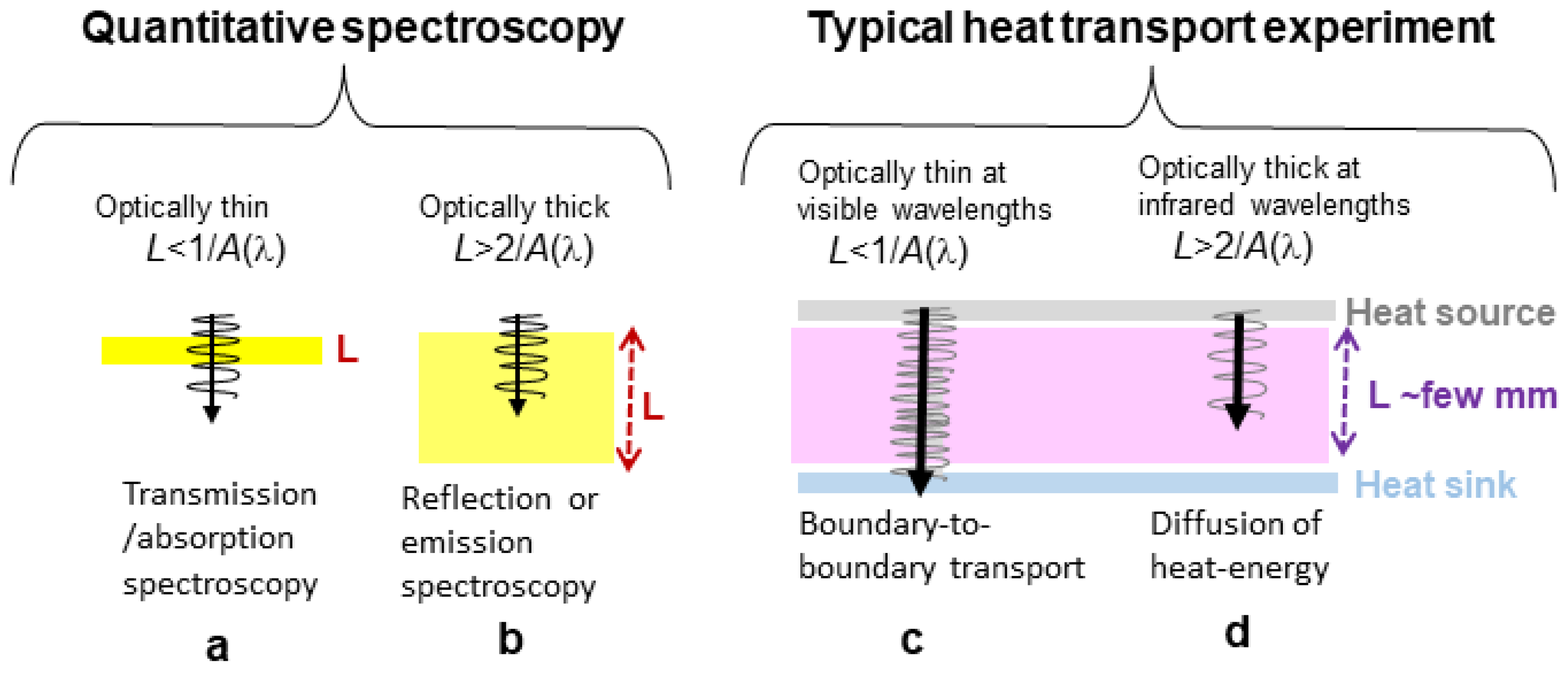
  • Electrical insulators partially transmit light in the near-infrared (IR), and/or visible to ultraviolet (UV) ranges over the ~1–3 mm lengths (Figure 1a), which are typical of heat transfer experiments. Although spurious radiative transfer gains roughly offset contact losses near room T, this non-diffusive radiative contribution (Figure 1d and Figure 2a) increases to ~500% by 1000 K [16,17]. Grain boundary scattering reduces spurious radiative transfer, but does not eliminate this effect for thin and/or pale-colored samples [16,17].
  • Experimental errors are commonly ascertained from comparisons with metals, which typically yield ±5% experimental uncertainty. However, metals lack the systematic errors of contact losses and radiative gains that accompany measurements of insulators, so the actual uncertainty is much larger [5].
  • Modern methods for determining K, such as thermoreflectance, reach ±5% with difficulty [18]. Because the distance over which heat diffuses is not part of analyzing the raw data, benchmarking against previous work is essential, which makes thermoreflectance a lower accuracy, comparative method.
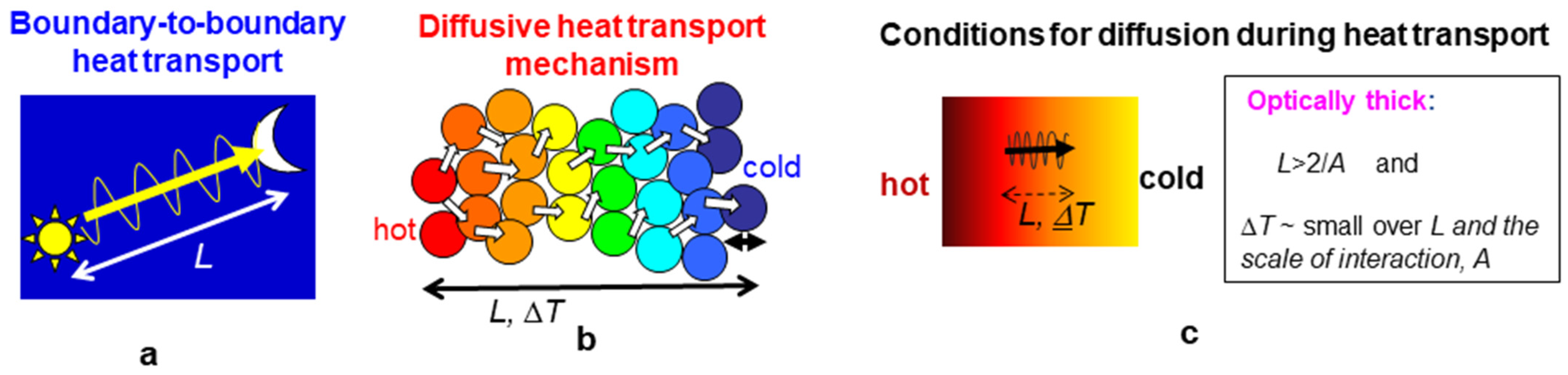
  • Light crossing a sample with negligible interaction (Figure 2a) is called boundary-to-boundary or ballistic radiative transport. This “direct” mechanism is not related to diffusion of heat (Equation (3)), since the latter requires participation of the medium (Figure 1c,d). Because direct radiative transfer is familiar, qualifiers (e.g., “ballistic” or “boundary-to-boundary”) are often omitted, leading to misunderstandings. Thin, pale-colored samples are particularly affected. Sometimes, a T3 formulation for K was inappropriately used to remove unwanted radiative transfer (e.g., [8,19]). However, this formula represents diffusion of radiation, e.g., through large expanses of matter (glass vats: [20]). Moreover, this formulation describes a greybody, not a partially transparent mineral (e.g., [5,21]).
Figure 1. Schematics comparing spectroscopic to heat transport experiments. (a,b) Optically thin vs. optically thick conditions require different types of spectroscopy measurement at a given wavelength (λ). The absorption coefficient, A = −ln(Itransmit/Iincident)]/L where L is thickness, describes attenuation of light with intensity I. Squiggly arrow shows the direction of light and whether it crosses the sample (yellow block) or not. (c,d) Behavior during heat transport experiments where the heat source (grey bar) provides heat (blackbody radiation) over a wide range of λ. Typically, the visible part of the blackbody curve crosses mineral samples (pink rectangle) with little attenuation, reaching the heat sink or thermocouple (blue bar) and warming it. Modified after Criss and Hofmeister [22] (their Figure 4) which has a Creative Commons license.
Minerals 16 00509 g001
Figure 2. Schematics illustrating the two mechanisms of radiative transfer and when these occur. (a) Boundary-to-boundary radiative transfer, where light (yellow arrow) from a source (the Sun) passes through an optically thin medium (space, distance L) with negligible interactions and then heats a sink (the Moon). (b) Diffusion, which consists of progressive absorption and re-emission of heat or light (white arrows) down a temperature gradient. The medium may consist of atoms or grains (small double arrow). Diffusion occurs only at wavelengths where optically thick conditions exist. (c) Schematic defining optically thick conditions in a temperature gradient. “Small” depends on the temperature dependence of the material’s absorption coefficient and on the thermal gradient. If ΔT is very large over some distance L, then the radiation can cross L without interacting with the intervening medium, so the heat is not diffusing. Modified after Criss and Hofmeister [22] (their Figure 6) which has a Creative Commons license.
Minerals 16 00509 g002

1.1. Purpose and Organization of the Present Study

To improve understanding of heat transport in structurally complex and chemically variable serpentine minerals, this paper provides accurate (within ±3%) laser flash analysis (LFA) measurements of D vs. T, which lack systematic experimental errors of contact losses and ballistic radiative gains (e.g., [23]). Section 2 provides background and theory. Section 2.1 summarizes the laser flash and thermoreflectance methods. Section 2.2 covers recent theoretical developments on the dependence of heat transport properties on P, T, and mineral proportions of rocks.
We provide LFA data to high temperature of oriented sections of near-endmember antigorite and chrysotile, and of lizardites with diverse chemical compositions, some of which were measured in three perpendicular directions. Available information on cP and ρ is summarized, evaluated, and utilized to more accurately calculate K from D (via Equation (5)) than can be achieved through direct measurements of K. A thermodynamic identity is used (with elastic moduli data) to accurately provide K−1K/∂P. Samples with thickness > ~1 mm are investigated here, to provide D (or K) values that are relevant to macroscopic behavior (Section 2.1).
Lizardites with low amounts of Fe are the focus, as these are abundant. Charge state and speciation of Fe are characterized using visible spectroscopy, which also probes whether Cr3+ enters tetrahedral sites [24].
Dehydration was not quantified in previous heat transport studies. Thus, infrared spectra and x-ray diffraction data were measured for starting material and run products.
Section 3 describes materials and methods. Section 4 gives the experimental results. Section 5 calculates K from LFA data. Section 6 discusses mineralogical and geophysical implications. Section 7 concludes.

1.2. Key Findings of the Present Study

Our accurate LFA data on transport properties differs from previous contact studies by ~30% at ambient conditions. Previously reported pressure derivatives err by factors of 2 to 5, attributable to deformation of soft serpentines. Previous temperature derivatives are corrupted by ballistic effects and ineffective attempts to remove these. Unaccounted for two-dimensional heat flow also artificially elevates D or K. Our data pave the way for accurate thermal models of slab and upper mantle environments.

2. Background and Theory

2.1. General Discussion of Heat Transport Properties and Their Measurement

2.1.1. Laser Flash Analysis and the Importance of Length-Scale

Laser flash analysis [25] measures D with a high degree of accuracy (~±3% or better): see reviews of [23,26]. This method is contact-free, since samples are suspended by their edges, heat is remotely supplied, and sample temperature is remotely monitored with an IR detector (analogous to Figure 1c,d). LFA is based on measuring the time-dependent changes in temperature on the near side of a sample of known thickness (L), after a brief heat pulse is applied to the far side. Solutions to Equation (4) take on the forms required by dimensional analysis:
D     L 2 / τ   or   D ~ u L .
where τ is a time constant with an associated characteristic speed of u = L/τ. Parker et al.’s [25] adiabatic model for LFA provides the left-hand side (LHS) of Equation (6) with a numerical proportionality constant of 0.138785 mm2 s−1, where τ = t½, is the time needed for sample emissions to reach ½ of the maximum temperature increase following a heat pulse.
Importantly, Fourier’s description of heat diffusion requires the following:
  • Equation (6) indicates that D depends on thickness, asymptoting to D ⟶ 0 as L ⟶ 0, which is consistent with diffusion requiring a medium.
  • The linear dependence of D (and thus K, per Equation (5)) on sample lengths below ~0.5 mm for oxides has been experimentally verified [27,28,29]. The implied mechanism, diffusion of infrared radiation, has been quantified for metals, graphite, and a simple oxide, corundum [5,29].
  • For L > ~1 mm, D is independent of L under temperatures accessed in the laboratory. In this case, heat diffusion involves both IR fundamentals and overtones [5,29], whereas visible radiation provides the spurious boundary-to-boundary component that corrupts data from contact methods (Figure 1c,d).
Thus, LFA experiments on mineral samples with L > ~1 mm represent diffusion of heat in geological environments at high (<~2000 K), but not extreme, T.
It is the simplicity and robust nature of the LFA method which provides versatility and continued developments [23]. Regarding mineral and glass studies, key advances were (1) reduction of radiative transfer gains in LFA experiments through applying thin coatings of graphite or metal to the sample [30] and (2) removal of remnants by mathematically modelling the raw data (time-temperature curves) [31,32,33]. These models are based on negligible participation of the medium when energy is transferred across the sample (Figure 2). Blumm et al. [34] describe the basics of this class of models, which require no knowledge of optical properties.
Elimination of boundary-to-boundary transport from LFA results means that diffusion of heat (Figure 1d and Figure 2b,c) is quantified, which is governed by Fourier’s laws, Equations (3)–(6).
Much confusion exists because visible radiation can diffuse at high temperature, i.e., in Earth’s mantle where T changes slowly over large distances (Figure 2c). Diffusion requires that the sample is optically thick at frequencies associated with the blackbody curve at that temperature and for the sample thickness used in that particular measurement (or environment). Ballistic transport involves optically thin conditions, where light crosses the sample with negligible interactions (Figure 2a). Effects of optically thick conditions vs. optically thin conditions in the laboratory, planetary, and astronomical settings are discussed further by [22,35].

2.1.2. Thermoreflectance Uncertainties and Limitations

Thermoreflectance relies on complex, multi-parameter modelling. For a brief description and references, see Zhao et al. [18].
Sample thickness is not an important component of thermoreflectance modelling, as this technique was developed to study thin films with unknown thickness. Yet, from Equation (3) and its solutions, which follow the form of Equation (5), thickness controls numerical results for D and K [5,28,29].
Despite thermoreflectance probing thin films, the dependence of D or K on thickness has not been mentioned. Benchmarking against 10 to 100 times thicker samples prevents recognition of the thickness dependence required by dimensional analysis (Equation (6)). Because thermoreflectance is based on multiple, free parameters, tweaking achieves “agreement” between samples with dissimilar length scales. Problems with pressure derivatives from thermoreflectance of basaltic glass [36] are discussed by [37].

2.2. Theoretical and Empirical Descriptions of Transport Property Variations

2.2.1. Thermodynamic Identities Provide the Pressure Responses of K, CP, and D

Because any amount of energy can occupy a given space, ℑ is independent of pressure. Hence, taking the P derivative of Equation (3), LHS relates ∂K/∂P to thermodynamic parameters [27,38]. Note that linear thermal expansivity, αlinear ≡ (1/z)∂z/∂T|P, is a scalar quantity. Its typically positive sign requires a positive sign for the thermal gradient, ∂T/∂z. However, a negative temperature gradient (∂T/z) is associated with positive signs for ℑ and K in Equation (3). Maintaining consistent signs for both K and α during algebraic manipulations gives the following:
1 K K P T = 1 V 1 / 3 V 1 / 3 P 1 α α P   = 1 B T 1 3 + δ T ,   where   δ T = B T α α P = 1 α B T B T .
and where V is volume, BT is the bulk modulus (inverse of compressibility = (1/V)∂V/∂P), and α is the volumetric thermal expansivity = (1/V)∂V/∂T. The second Grüneisen parameter (δT) is close to 6.5 for diverse materials if assessed using data on α/∂P [39] or to 7 if more accurate data on ∂B/∂T are considered [27,28,40].
Another identity, derived from the definition of cP as the response of a material to adding heat (Qext) by [40], pertains to the following:
1 c P c P P T = 1 B T 1 Q ext M c P 1 B T B T T 1 B T .
The dimensionless term B−1∂B/∂T is ~10−4 whereas Q/(McP) is ~1. Taking the P derivative of Equation (5) and then inserting Equation (8) yields the following:
1 D D P T = 1 K K P T   .
For completeness, we note that only one bulk modulus exists theoretically, which is confirmed by accurate experimental data [40].
The above equations were experimentally confirmed [27,28,40]. Thus,
  • LFA data on D(T), combined with information on B, ρ, and cP, provide a complete and accurate description of K and the process of thermal transport.

2.2.2. Empirical Dependence of Thermal Diffusivity on Temperature

This simple formula:
D ( T ) = F T G + H T  
describes a large (~300 substance) database on crystals (including several mineral families), glasses, metals, and rocks previously measured using LFA up to melting ([5,41,42]). The FTG term represents diffusion of low-frequency IR light, connected with fundamental vibrational modes, whereas the HT term represents diffusion of light at higher frequencies, e.g., weakly absorbing overtones in the near-IR [5,29]. For both cases, heat transfer occurs via progressive absorption and reemission of light along the path (Figure 2b).
  • Although a power law may describe data collected on many substances up to 800 K, as well as simple diatomics and some elements, reproducing high T data requires the HT term [5,41].
  • From measurements of refractory minerals (e.g., olivine [16]), Equation (10) holds up to 2000 K. Thus, temperatures where serpentines occur are represented.

2.2.3. Sum Rules for Slowly Varying Temperature

Steady-state flow of heat across layers which are perpendicular (⊥) to the direction of flow is long understood since the same applied flux ℑ pertains to each interface [43]. If layer thickness varies, a series is represented by the following:
L K = L j 2 C j K j 1 L i C i = L i K i   .
If the Ci’s are similar for the layers, then a harmonic mean also holds for D.
Early descriptions of parallel (||) flow as K|| = ΣKi originate by analogy to electrical currents, see [43]. This analogy is inappropriate because heat, unlike charge, flows into, across, and out of any solid.
Equations for heat flow in parallel bars of equal area were derived by Criss and Hofmeister [44] from Fourier’s laws by conserving heat-energy (the adiabatic approximation). The resulting summation, KΣCiTi/∂zi = CΣKiTi/∂zi, was simplified to account for common relationships among the component storativities (Ci = ρicPi) and diffusivities (Di). For n independent mechanisms, C = ΣCi, in equal area bars. Allowing for different cross-sectional areas of the bars leads to:
K | | = f i C i K i C i =   f i C i K i C  
where the volumetric fractions (fi) sum to f = 1. Essentially equal Ci values provide the arithmetic mean.
Regarding rocks, both series and parallel flow occur during heat transfer. Thus, Merriman et al. [42] averaged Equations (11) and (12), while replacing Li/L in Equation (11) by fractions fi. When the heat capacities of phases are similar, as is typical of minerals above 700 K, the LHS of Equation (13) holds, where:
D =   1 2 f i D i + 1 2 f i D i 1 ;   for   monomineralic   rocks   D = 1 6 D 1 + D 2 + D 3 + 3 2 1 D 1 + 1 D 2 + 1 D 3 1
For monomineralic rocks, the LHS reduces to the RHS. Data on low porosity rocks [42] confirm Equations (11)–(13).

3. Experimental Methods and Materials

Methods are summarized below. For details, see, e.g., [5,16,17,28,37,41,42,44].

3.1. Samples and Sample Preparation

Samples from the departmental collection at Washington University and the Smithsonian were supplemented by purchases from Excalibur minerals, Charlottesville, VA, USA (Table 1).
For LFA, disks were sawed from portions of the sample that appeared to be monomineralic and then were ground into disks of 6 to 15 mm diameter with 0.7 to 1.55 mm thicknesses and nearly parallel surfaces. Antigorite was oriented in accordance with crystal faces. Blocky lizardites were cut in perpendicular directions. To keep fibrous chrysotile samples intact, thicker (2.5 to 3 mm) samples were used perpendicular (⊥) to the tubules (the a-axis), whereas 8 mm lengths were needed for measurements parallel (||) to a. The platy habit and bright green color of pecoraite were used to extract this phase for LFA. Grains of Ni-Fe-lizardite, studied via spectroscopy, were too small for LFA measurements.
For electron microprobe analysis (EPMA), polished chips were examined. Spectra were obtained from chips and from LFA disks. X-ray diffraction data (XRD) were collected from powder of bulk samples, and from disks post LFA runs, which were powdered in some cases.
Thicknesses (L) of disks and chips were measured using a digital micrometer and/or a calibrated binocular microscope. Faces were polished for spectra and EPMA.

3.2. Chemical Analyses via EPMA and Inferred Formulae

Samples were characterized by wavelength dispersive analysis and standard procedures using a JXA-8200 electron microprobe (JEOL, Akishima, Tokyo, Japan). “Probe for Windows” was used for data reduction (http://www.probesoftware.com/). The CITZAF correction after Armstrong [48] was used. Various oxide and silicate standards were used for calibration, as detailed in [37]. Uncertainties are generally ±2%, but depend on concentration [49].
Mostly F and Cl have been neglected in performing chemical analysis (e.g., [2]). Fluorine contents in existing data on serpentines [50,51] are below 300 ppm. Because the highest value is near the limit of detection in EPMA of ~0.05 wt%, and little Cl was detected, the low totals are attributed to undetected hydroxyl.
Formulae in Table 1 were constructed by first allocating Fe3+ (and Cr3+) to the tetrahedral site, per spectral assignments. If Fe3+ remained, it was allocated to the octahedral site. Then, Al3+ was divided between the octahedral and tetrahedral site. When ambiguities existed, Fe3+ and Al3+ were evenly divided. For S1, charge balance that included excess OH provided a small amount of Fe2+, consistent with spectra.

3.3. Visible and Infrared Spectroscopy

Unpolarized ultraviolet (UV) to visible spectra from 190 to 1100 nm (9090–52,630 cm−1) were collected using a double-beam Shimaduzu UV-1800 (Shimaduzu, Kyoto, Japan) with 1 nm resolution. Identical apertures were used in the sample and reference beams. The bulb change at 340 nm induces a stair step. The UV portion was shifted slightly upwards to match the visible region.
For lower frequencies (~2000–8000 cm−1), a Bomen/ASEE Fourier transform infrared (FTIR) spectrometer (Bomem Inc., Quebec, QC, Canada) was used with an InSb detector and a CaF2 beamsplitter. Data on thin samples were collected from (~500–5000 cm−1) using an HgCdTe detector and a KBr beamsplitter. Samples were placed on an aperture, which was used by itself to provide the reference spectrum.
Absorption coefficients (A) were calculated from the standard convention used in the mineralogical literature and in programs for commercial spectrometers:
A L = log I t r a n s I 0
where I0 is the incident intensity, determined by measuring throughput across the aperture under the same conditions, and Itrans is the measured intensity. Reflections are not accounted for in the present work. Instead, as is typical in studies of the O-H and visible regions, baseline corrections are used.

3.4. Ascertaining Charge State and Site Occupancy

To minimize ambiguities in constructing formulae from microprobe analyses, site location for Cr and charge states and site location for Fe are inferred from comparing our visible spectra to previous studies (Section 4.2). Then, Al3+ is allocated to either or both the octahedral (M) or tetrahedral (T) sites to balance charge (Section 4.3). Table 1 provides these best estimates.

3.5. Powder XRD and Rietveld Analysis

Data were collected from powders (either 0.25 or 1 g) or the actual disks used in LFA, using a Bruker D8 ADVANCE X-Ray Diffractometer (Bruker Corp, Billerica, MA 01821, USA) with a vertical goniometer using Cu-Kα radiation, a position-sensitive LynxEyeXE dectector, and Bruker’s program Diffrac.Eva, version 7. Operating conditions were 35 kV and 35 mA. Scans were made from 2° angles of 5 to 60° or more. Step-size was 0.02° with scan times of 0.5 s per step. Background was removed using a polynomial fit.
The mineral phases present were determined using the Bruker software package Eva, which provided phases similar to those observed in EPMA. EVA matches peak positions in the XRD spectrum with those in the International Centre for Diffraction Data (ICDD) subscription database, version PDF-5+.
Mineral abundances in weight percent were then determined via Rietveld analysis [52], which is basically a structural refinement method [53]. We used the Bruker software package Topas, version 5, and literature data (structure refinements) on the phases detected using EPMA and the EVA program. The same reference data on antigorite, chrysotile, lizardite, and olivine were used in each refinement. Crystal size is determined from the breadths of the XRD peaks [54], and is not perceptibly affected by grinding. As breadths reflect behavior of interatomic planes (~20 nm), the obtained phase proportions and crystal sizes describe the mineral mixture.

3.6. Thermal Diffusivity Measurements

Two somewhat different instruments were used. Both are manufactured by Netzsch Gerätebau (Selb, Germany).

3.6.1. High Temperature Runs

In the LFA 427 apparatus, specimens are held in a graphite furnace under a dried Ar gas atmosphere. The temperature dependence of D is obtained by varying the furnace temperature, which is measured to within ~1 °C using a calibrated W-Re thermocouple. A laser pulse supplies a small amount of heat to a graphite basal coating on the sample, which also buffers oxygen fugacity. As this increment of heat diffuses from the bottom coat to the top graphite coat of the sample (Figure 1d), the time-dependence of thermal emissions is recorded with an InSb detector. The top coat enhances emissions. Data were obtained at 50–100 °C intervals with ~three acquisitions at each temperature which take a few seconds, and 1 min between acquisitions. Heating rates varied from 8 to 18 K per minute, and stability was reached before each acquisition, as confirmed by repeatability among the 3 data points. At ambient temperature, ~9 datapoints were collected to improve accuracy. Runs typically take a total of 6 to 8 h.
Data were processed using the algorithm of Mehling et al. [33] to extract thermal diffusivity from the time-dependent emissions. This model accounts for radiative surface losses from the sides and top to the surroundings and spurious radiative transfer through the sample between the top and bottom graphite coats, and allows for absorbance being frequency dependent, although the detailed values of optical properties are not needed. The measured shape of the laser pulse is accounted for [55].
Thermal diffusivity is accurate to better than ±3%, as verified against opaque reference materials (e.g., iron, steel, graphite and pyroceram, see [6,16,17]). Uncertainty in D arises from uncertainties in thickness and in slight departures from parallel faces. Hence, the precision within any given run is much higher, so the temperature dependence of D is better constrained than the absolute values of D.

3.6.2. Runs Below 500 °C (775 K)

An LFA 467 with a 0.01 ms pulse from a xenon flash lamp at 250 volts was used to collect room temperature data on run products, and to measure D vs. T for samples as small as 6 mm across. Here, 3 to 6 data acquisitions were used.
The LFA 467 has a HgCdTe detector to reach lower temperatures and uses focusing optics to study smaller samples. Purge gas flows continuously. Min et al. [56] provide details on the 467 model. We used a single sample in each of the 4 possible positions, which gives the highest possible accuracy, ~1% for runs on thin samples, based on results for copper and electrolytic iron standards. Obtaining D parallel to chrysotile tubules required using overly long samples. Accuracy for these two runs is lower: Section 4.5 gives details. Again, T derivatives are more accurate than initial values.
Most time-temperature curves were closely fit by the model removing radiative transfer [31,32,33,34]. But, for some samples measured after a heating run, the penetration model [57] provided a better fit. This behavior is explained by differential expansion of fine-grained serpentinites. Differences in D between these two models are within 1%.

4. Results

4.1. Chemical Composition from EPMA

Table 2 lists oxide contents for the main phase in each sample, which describe the disks used in LFA. Total iron contents are low, <3 wt% total FeO, except for Ni-Fe-lizardite, which was too small for LFA measurements. Wet (bulk) chemical analyses of chrysotiles [58] are similar to EPMA data for Globe, AZ, chrysotile, but include magnetite, as evidenced by 1 wt% Fe2O3 for their Thetford, Canada, sample.
Chips from most samples were single-phase. A light green portion (S2) of Snarum serpentine had many tiny calcite veins and so was not studied further. Darker green S1 had large calcite veins which were avoided in preparing disks for LFA. The two serpentine phases in the pecoraite rock are as described previously [3].

4.2. Visible–UV Spectra of Fe, Ni, and Cr Electronic Transitions

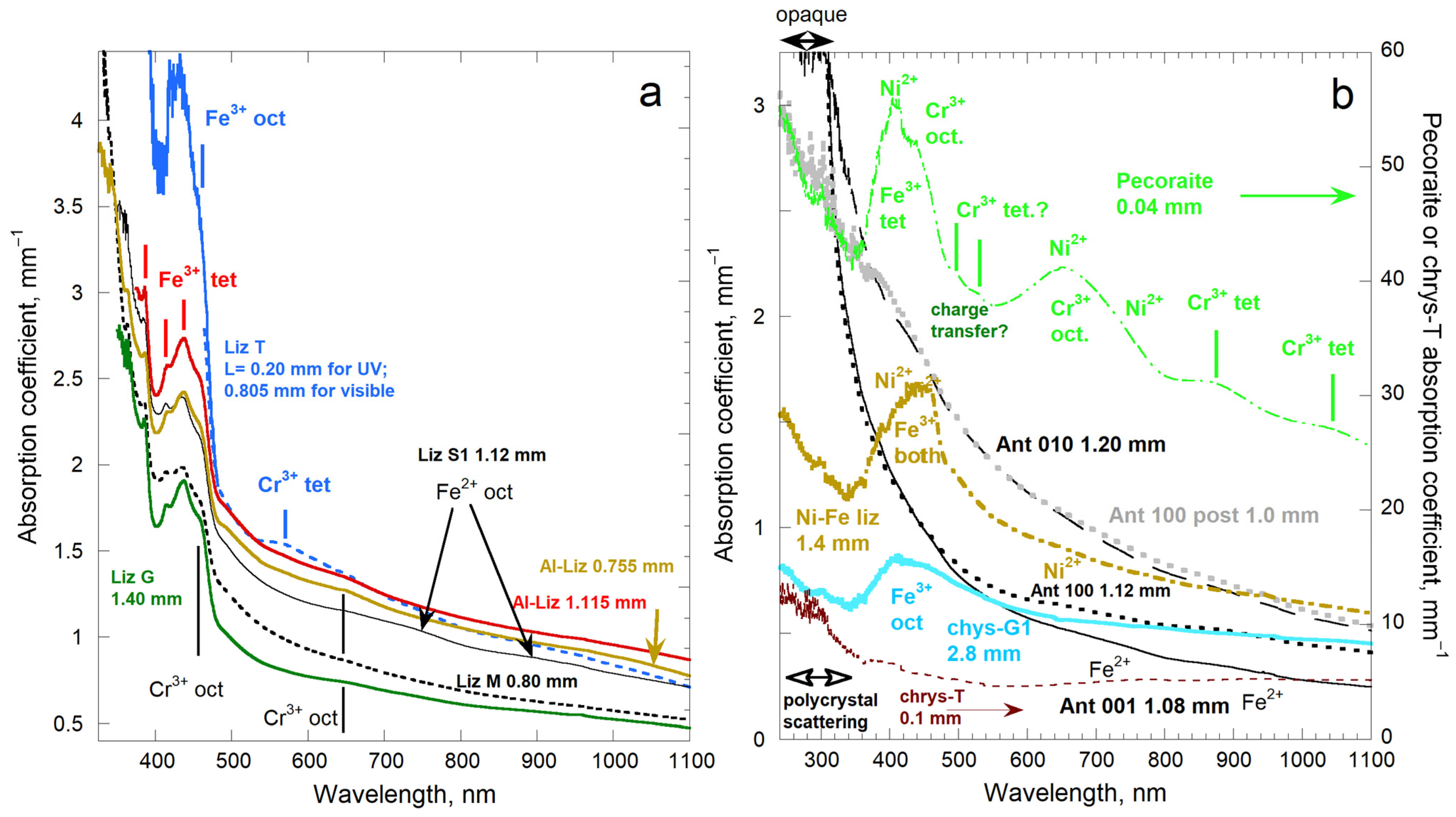
Figure 3 shows optical spectra of our samples before heating. Spectra of run products had strong physical scattering that prohibited acquiring accurate data below 400 nm, except for colorless regions (e.g., antigorite 100 in Figure 3b). Scattering is also evident in some starting material, specifically the Ni-Fe-lizardite, which had inclusions, and both chrysotiles, which are composed of tubules with cross-sections of ~0.1 mm × 0.1 mm. Band assignments in Figure 3 are based on previous spectra [59,60,61,62,63], see Appendix A.

4.3. Fe Charge State and OH Content

Table 1 lists formulae based on results from Section 4.1 and Section 4.2, and band assignments (Appendix A). From visible spectra, iron is mostly trivalent. Lizardites with substantial Fe2+ either have high Cr content (e.g., in the tetrahedral site of Liz-T) or with the presence of impurity phases (serpentines-S and -W).
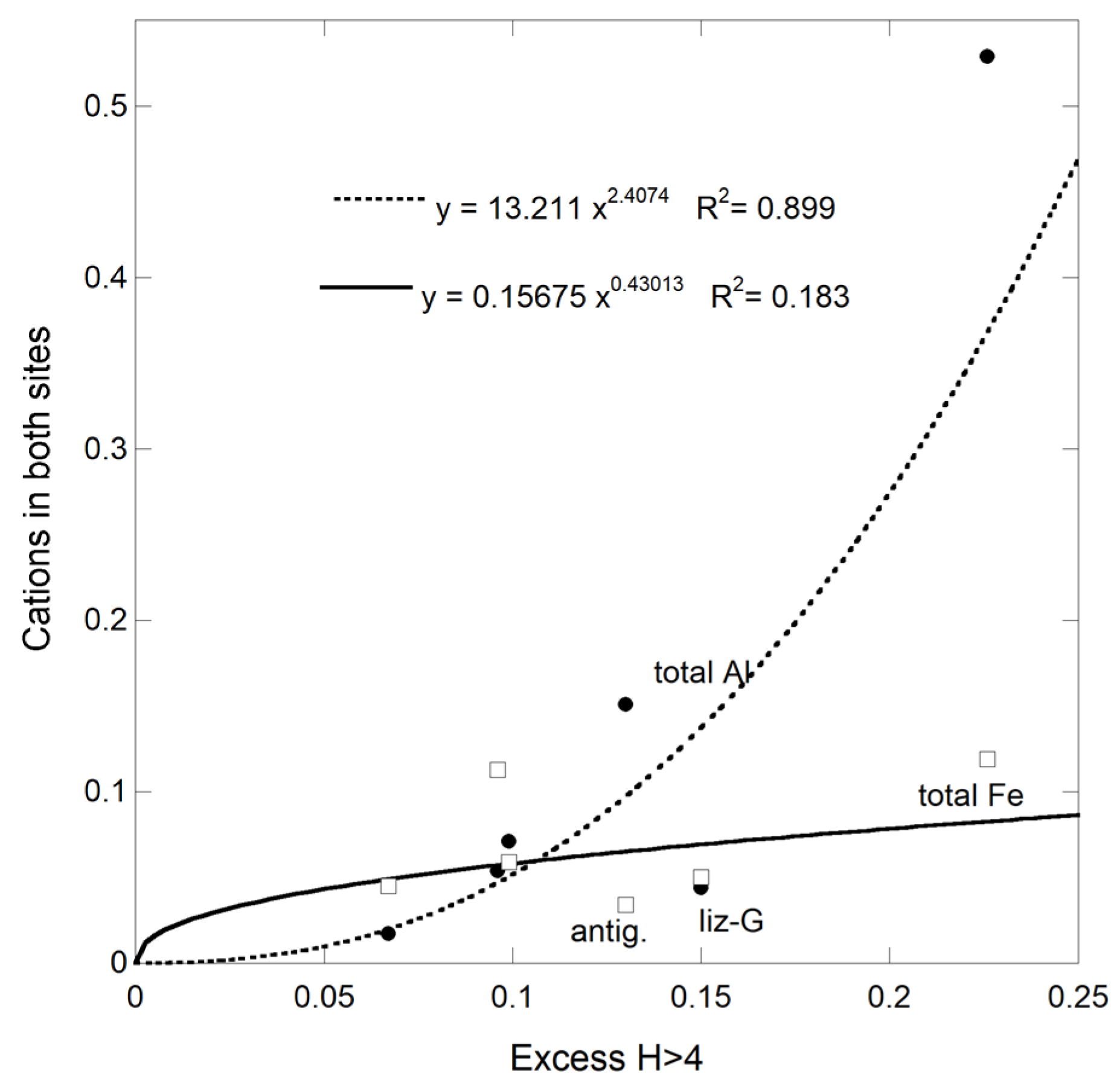
Except for chrysotile-G1, which is the closest to the Mg endmember, the single phases have OH slightly in excess of the ideal value of 4 in the serpentine formula. Total oxides lie below 99.1 wt%, so this excess is not due to overestimating water content. Both Cl and F occur in low amounts (Table 2), so these are not relevant to excess OH. The amounts of total H2O in Table 2 were chosen to provide good stoichiometry. Excess OH thus describes most of our suite. Based on EPMA data (Figure 4), we propose that the following charge-coupled substitution occurs in serpentine minerals:
Al3+ + OH ⟶ Si4+ + O2−
This substitution is known in quartz [64], and furthermore stabilizes the tridymite polymorph [65]. The extra H in serpentines could be located at sites joining the layers or in regions of layer mismatch. Although substitution of trivalent ions in the octahedral site contributes to charge balance, it is not sufficient in a few cases as indicated by the formulae in Table 1.

4.4. Structure and Impurities from XRD of Starting Material and Run Products

Large samples were powdered for XRD. This constrains the mineralogy of the bulk samples, and shows that the common impurity phases of magnetite and brucite are present at the % level (Table 3). Preferred orientation contributes to the uncertainties.
Disks for LFA were cut of portions that appeared translucent. Most of the heated disks only had forsterite or the main lizardite 1T phase, suggesting that large amounts (>5%) of impurities were avoided in LFA measurements. Small amounts of impurities are not precluded, and are likely present in variable amounts in several samples: Disk #3 of the bright yellow Al-serpentine contained brucite, as did the powder. Serpentine-W had both lizardite and chrysotile, with calcite veins throughout (Table 3).
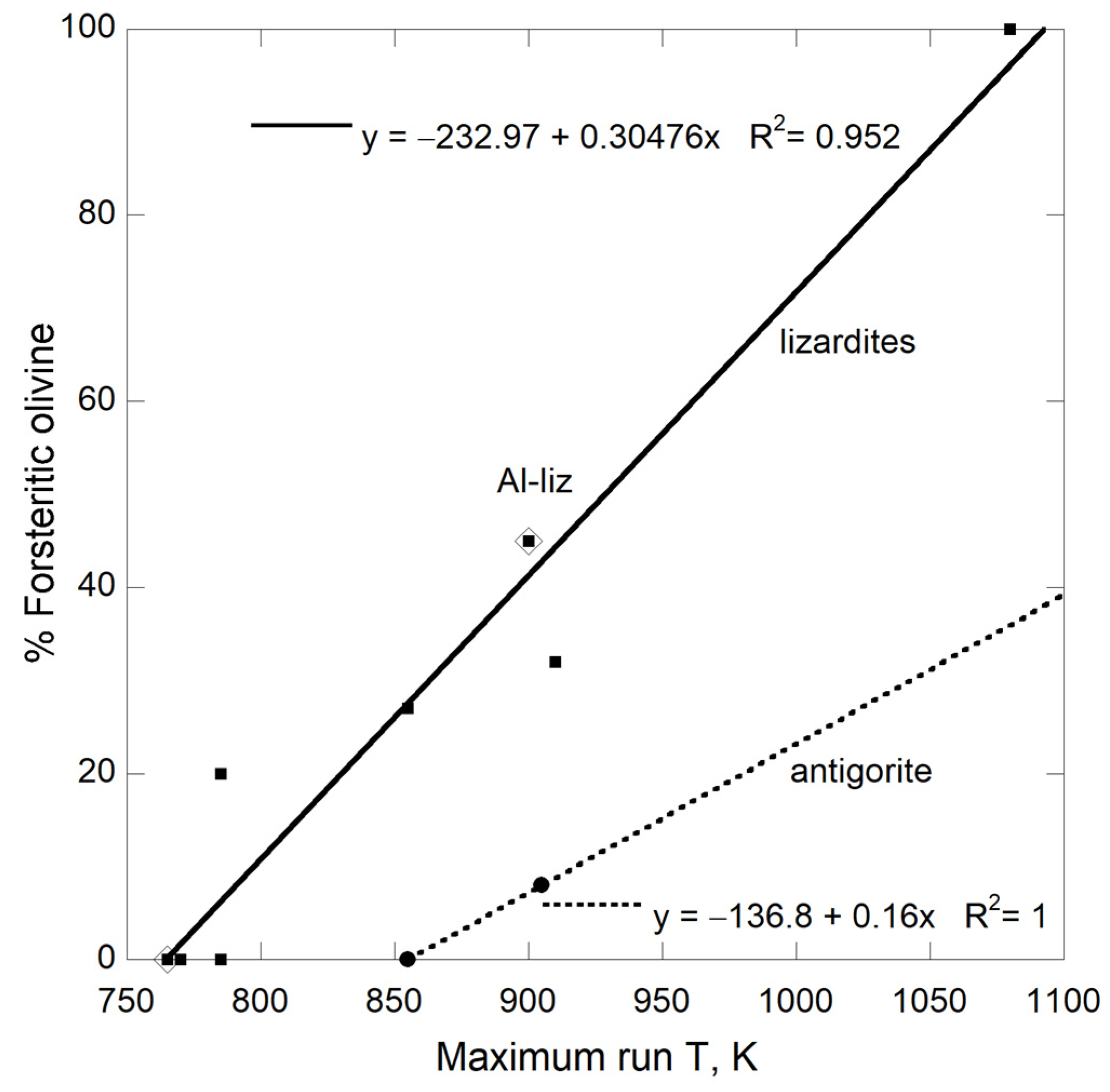
The run products have variable amounts of forsterite, which depends on the maximum temperature of the runs (Figure 5). The heating rate is ~5 K min−1 overall where each set point involves ~5 min of data collection at a fixed temperature after thermal stability is achieved. Variations in hold time plus uncertainties in refinements are consistent with the scatter. In any case, dehydration of the fine-grained lizardites begins by 800 K, whereas ~900 K is required for crystals of antigorite. Chrysotile samples were not heated above 770 K. Linear trends (Figure 5) indicate gradual decomposition of serpentine minerals with time during our experiments. Sixty minutes was sufficient to fully transform the samples in the laboratory. So, in a geologic setting, where the rocks sit at high temperature for longer times, the reaction would go to completion at lower temperatures. For this reason, only D and K for serpentines at T below ~800 K are used here.
Grain sizes of the olivine run products ranged from 30 to 62 μm. This size did not vary appreciably with the maximum T.
Figure 5. Proportion of forsteritic olivine in samples partially decomposed during LFA runs. Heating from ~770 to 1080 K took ~60 min.
Minerals 16 00509 g005

4.5. Near-Infrared Spectra of Antigorite and Lizardite

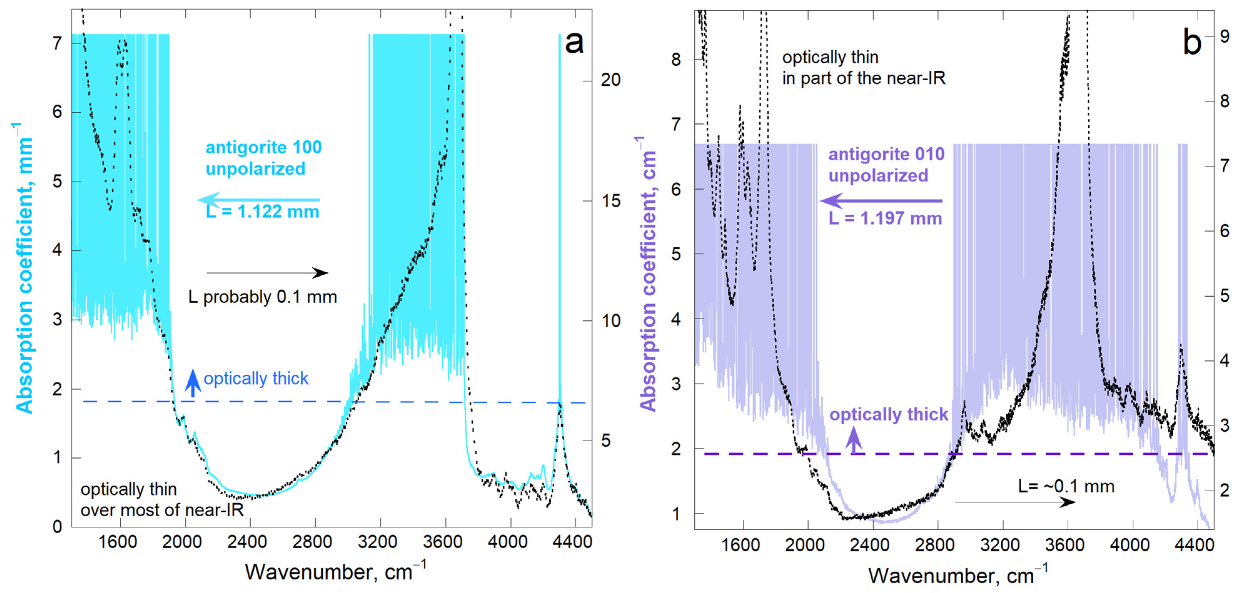
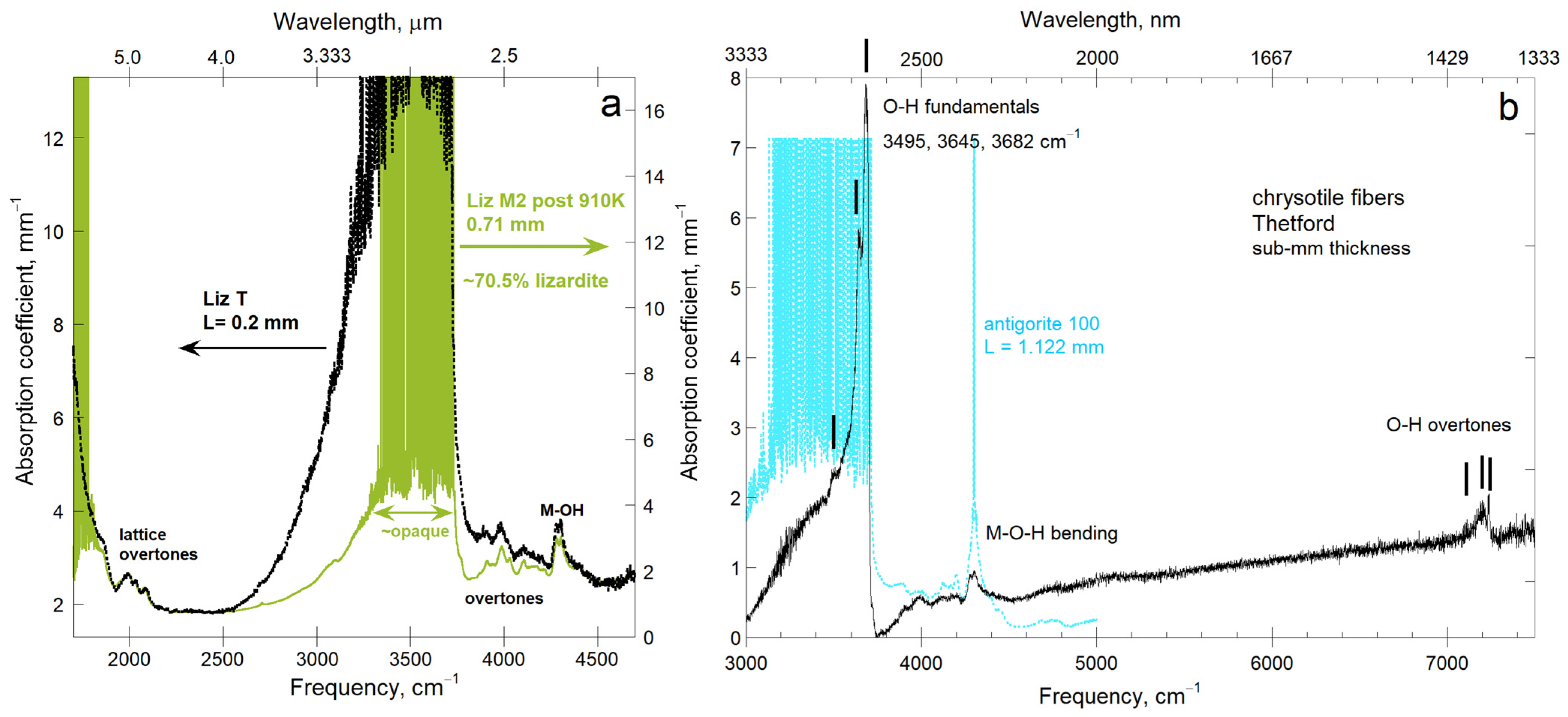
Near-IR spectra were obtained from ~mm thick slabs used in LFA measurements, and compared to spectra from chips with L near 0.1 mm. Antigorite single-crystals (Figure 6) lack internal reflections at grain boundaries. The (001) face provided similar results to (100), see below. Lizardite and chrysotile spectra (Figure 7) are similar to antigorite. Absorptions are strong near frequencies of 3000 to 3600 cm−1 (λ~3.3 to 2.8 μm) due to large amounts of stoichiometric hydroxyl which produces an O-H stretching band. Several bands exist, as clearly shown for chrysotile (Figure 7b).
High A for the main O-H stretching band is also demonstrated in previous IR spectra of films of chrysotile and lizardite powders. The main O-H stretching mode is well-resolved even for films compressed to ~1 µm [66]. In [66], thickness and band strength were calibrated via comparison to powders compressed to either 6 or 12 µm, where thickness was controlled by a tin gasket. In Figure 6, chip thickness is confirmed by comparing peak heights that are well-resolved in spectra from thick and thin samples.
Thin film data are not provided on antigorite given the band strengths [66], and because the band strengths in the near-IR are similarly strong in chrysotile, antigorite, and lizardite (Figure 6 and Figure 7); also, see chrysotile IR spectra from L = ~0.5 to 1.5 µm in [5] (p. 56).

4.5.1. Overtone Region

For chrysotile, near-IR spectra were collected above ν = 5000 cm−1 (λ = 20,000 nm or 2 µm). From Figure 3 and in accordance with the low Fe2+ contents of our suite, our samples weakly absorb from 5000 to 10,000 cm−1 (λ = 1000 nm). Overtones of O-H stretching existing near 7200 cm−1 are weak, with strengths resembling the M-O-H bending modes. Three bands for the fundamental and overtones suggest that three sites exist.

4.5.2. Partial Dehydration of Run Products

Figure 7a compares Liz-M2, which partially transformed to olivine after attaining 910 K in LFA experiments, to a thin slice of the as received, compositionally similar Liz-T sample. The two near-IR spectra were scaled to match the overtones and M-OH stretching band. Forsterite has peaks at 1750 and 1900–1950 cm−1 [5] (p. 59) which are masked by the noise in the heated sample. Thus, Figure 7a measures the lizardite remaining in disk M2 after the LFA run. Scaling the absorption coefficients suggests that disk M2 is 70.5% lizardite. This value is within uncertainty of the Reitveld proportions of 68% lizardite and 32% olivine (Table 3). The main O-H stretching band was reduced by a factor of 2.6 (38%), which suggests that disk M2 is 62% lizardite and 38% olivine. This result is less certain, due to distortion of the O-H stretching band in ~mm thick samples.
All three measures of partial decomposition (overtone peaks, OH band intensity, Rietveld refinement) are compatible for run products of Liz-M2. Thus, XRD data (Table 3) suffices to ascertain partially transformation of the other samples (Figure 5).

4.6. Thermal Diffusivity

4.6.1. Overall Response of D to Temperature and Phase

Results from LFA show that thermal diffusivity of serpentine minerals is generally low at ambient temperature (0.55–1.5 mm2 s−1), except for chrysotile ||a, for which D = 4.5 mm2 s−1 (Table 4). As T increases, D decreases such that the slope ∂D/∂T also decreases, providing relatively flat trends by T~600 K (Figure 8).
Error bars for measurements of thin samples are smaller than the symbol for runs below 775 K using the LFA-467 and are 2 to 3% for the runs to higher T, using the LFA-427, as shown graphically in Section 4.6.3. For the very thick chrysotile samples, error bars provided by the software of the LFA-467 are shown. Values allow for heat flow losses from the sides. Regarding the thinnest samples, Liz-M and Al-liz have similar D values for small L = 0.79 mm and for typical L of ~1 to 2 mm, so the limiting behavior of Equation (6) does not occur here.
Several samples were explored above their stability limit. Dehydration and transformation of Liz-M1 to forsterite is recorded by a substantial decrease in D from ~825 K to 950 K, followed by constant D above 950 K (Figure 8a). Except for sample Liz-M1, maximum run temperatures were insufficient for complete transformation to forsterite (Table 3; Figure 6). Lizardite T, which contains two serpentine phases, has a much flatter trend at high T than liz-M sections.
The dependence of D on T for serpentine-S1a (Figure 8b) is almost identical to that of liz-T. Lizardite-T was too small for XRD evaluation. Previous XRD papers [45] state that “mostly lizardite” was present: thus, the second phase has a different structure. Serpentine-G with impurities follows a similar trend to those of liz-T and serp-S1a. Serpentine-W, which is mostly lizardite but with significant amounts of chrysotile and calcite, was oriented perpendicular to its fibers. The steep trend of serp-W is consistent with low D of chrysotile ⊥a (Figure 8c; Table 4), and a slight increase in the proportion of chrysotile ⊥a during the experimental run per XRD (Table 3). Due to high D of chrysotile||a (Figure 8d; Table 4), randomly oriented chrysotile impurities in lizardite would increase D of the mixture. Note that the strong upturns exist only above 800 K, where the phases are not stable. We infer the following:
  • The trends for Liz-M represent low-Fe lizardite ± magnetite up to dehydration whereas the trends for liz-T, serp-S1a, and serp-G represent a combination of lizardite with minor, probably randomly oriented chrysotile.
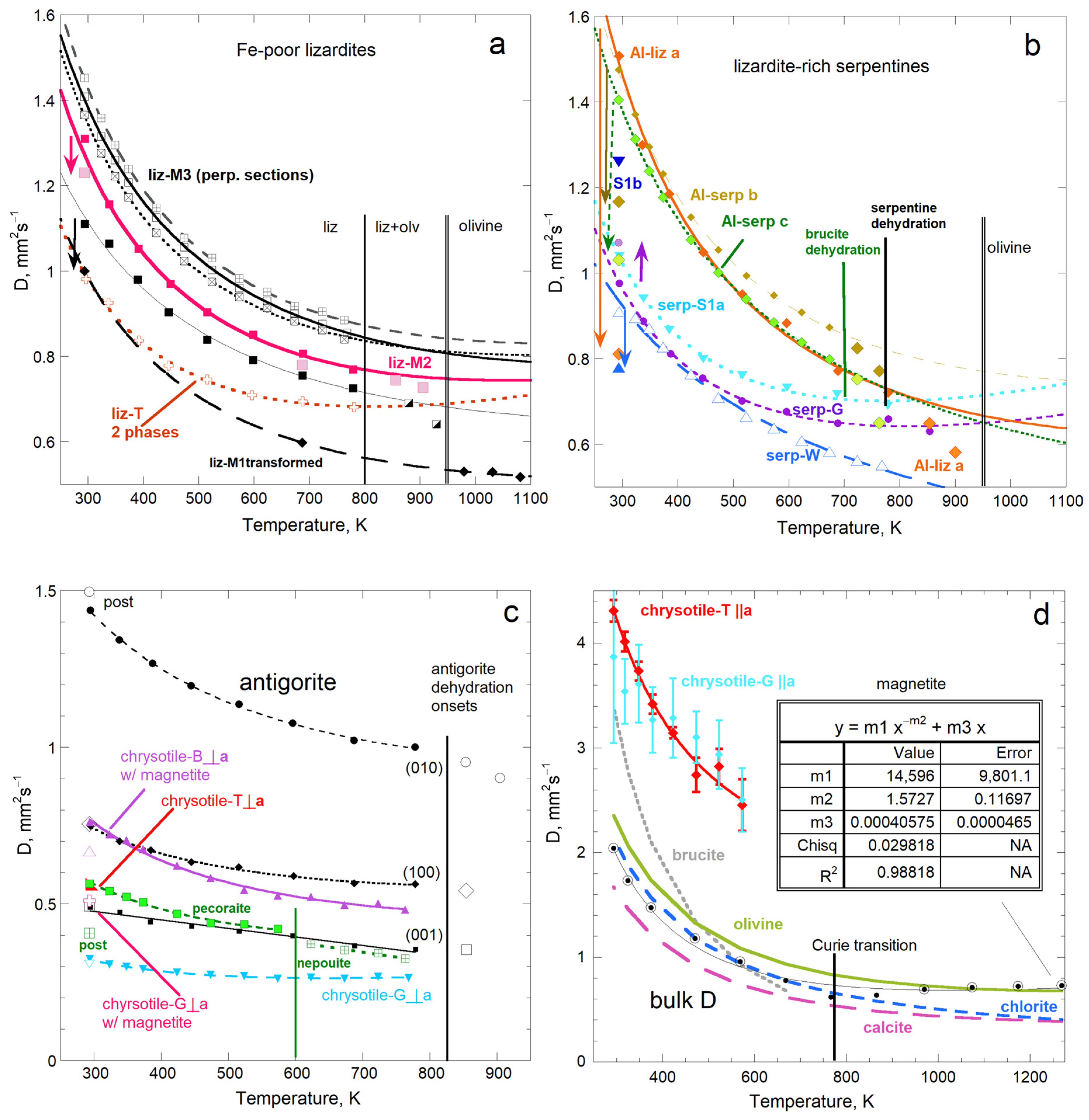
Figure 8. Thermal diffusivity as a function of temperature for various serpentines. Curves are least squares fits, listed in Table 4. Vertical lines indicate transformations. Vertical arrows show the direction of the change in D at 298 K after the run. (a) Lizardites near the Mg endmember. Lizardite M1 (filled squares) converted gradually between 800 and 950 K (half-filled squares) to forsteritic olivine (diamonds). Lizardite-M2 (pink squares) partially dehydrated. Three sections (M3abc: various open squares) were cut perpendicular to one another. Lizardite-T had two phases. (b) Al-lizardite and serpentines. Serp-S1a (filled triangles) and serp-G (purple dots) partially transformed to forsterite. Serp-W (open triangles) had more chrysotile in its run product. Sections b and c of Al-serp dehydrated at low T, confirming the presence of brucite. (c) Antigorite (black symbols, oriented as labelled) and chrysotiles ⊥a in various colors, as labelled. Open symbols indicate transformation, incomplete for antigorite. (d) Chrysotiles ||a and bulk D for the various impurity phases, as labelled. Experimental uncertainties (error bars) are larger than ±2% for chrysotiles||a because these samples were tall cylinders, not flat disks. Chrys-G also had the minimum diameter for our instrument, so fits are to chrys-T, with and without the linear term. Inset gives fits for magnetite omitting the Curie transition. Brucite, olivine, chlorite, and calcite data are respectively from [5,17,67,68].
Minerals 16 00509 g008
Dehydration of the Al-serpentine disk c begins near 700 K (Figure 8b), consistent with detection of 3 wt% brucite via XRD (Table 3). Losses of brucite are indicated by the powder having three-fold higher impurity content (9 wt% brucite). The low dehydration T of disk b shows that minor amounts of brucite are present, but all was converted given XRD results (Table 3). Disk a showed dehydration at 800 K, due to partial conversion to olivine, so brucite impurities were minimal: hence, disk a best represents D for Al-lizardite. Trends for all three Al-rich sections are steeper than those of liz-M slices.
Variations of D(T) for the three perpendicular orientations of liz-M3 and of the Al-serpentines are small. Similar trends indicate that random orientations of lizardite-rich samples reasonably represent bulk lizardite of the given composition.
Anistropy in D of antigorite is large, such that trends for D(T) are flatter for lower D at 298 K (Figure 8c). Dehydration begins near 825 K, as in Mg-rich lizardites.
Chrysotile has even greater anisotropy (Figure 8c,d). The presence of significant amounts of magnetite with D298 = 2 mm2 s−1 strongly influences Da but imperceptibly affects D for chrysotile||a, since the former is much smaller than magnetite D, while the latter is much larger.
Pecoraite transforms from the chrysotile to lizardite structure near 600 K (Figure 8c). Transformation results in very fine grain-sizes and changes in the oxide impurities. The presence of Fe2+ as magnetite in the run product suggests reduction occurred during transformation. Hence, the only quantitative measurement of Ni-serpentines is that of pecoraite at low T.
Notably, samples that transformed to olivine have much lower D near 1100 K (~0.55 mm2 s−1) than bulk olivine, where D is near 0.75 mm2 s−1. This difference remains in the recovered Liz-M. Exsolution of water and the fine grain sizes of the olivine run products (30–60 μm: Table 3) points to high porosity, which lowers D. In natural settings and over longer times than our hours-long experiments, porosity would be removed as water ascends. For this reason, these effects were not quantified, and post-run olivine data is not discussed further. Instead, olivine data from [17] are used below.

4.6.2. Fits to D vs. T

Below dehydration temperatures, D(T) is fit by Equation (10) for almost all samples (Figure 8; Table 4). However, the positive HT term is not needed to fit the (001) orientation of antigorite. This term probably exists, but is “buried” since over all T, (001) can also be fit by D = 0.5592 − 0.00027294T, with residual R2 = 0.969.
For low–T data on chry-T || c + mag, fits with and without the HT term were performed (Figure 8d). Including coefficient H provided a better fit (yielding G = 1.06) but F was poorly constrained. We therefore averaged G from fits with and without HT to provide the alternate fit in Table 4, which is our best representation of the data.
A linear fit describes the high-T data on nepouite (Table 4). The datum on the recovered sample with D = 0.407 mm2 s−1 is not used. During heating, grains preferentially expand, and so a multiphase sample may not return to the original configuration.
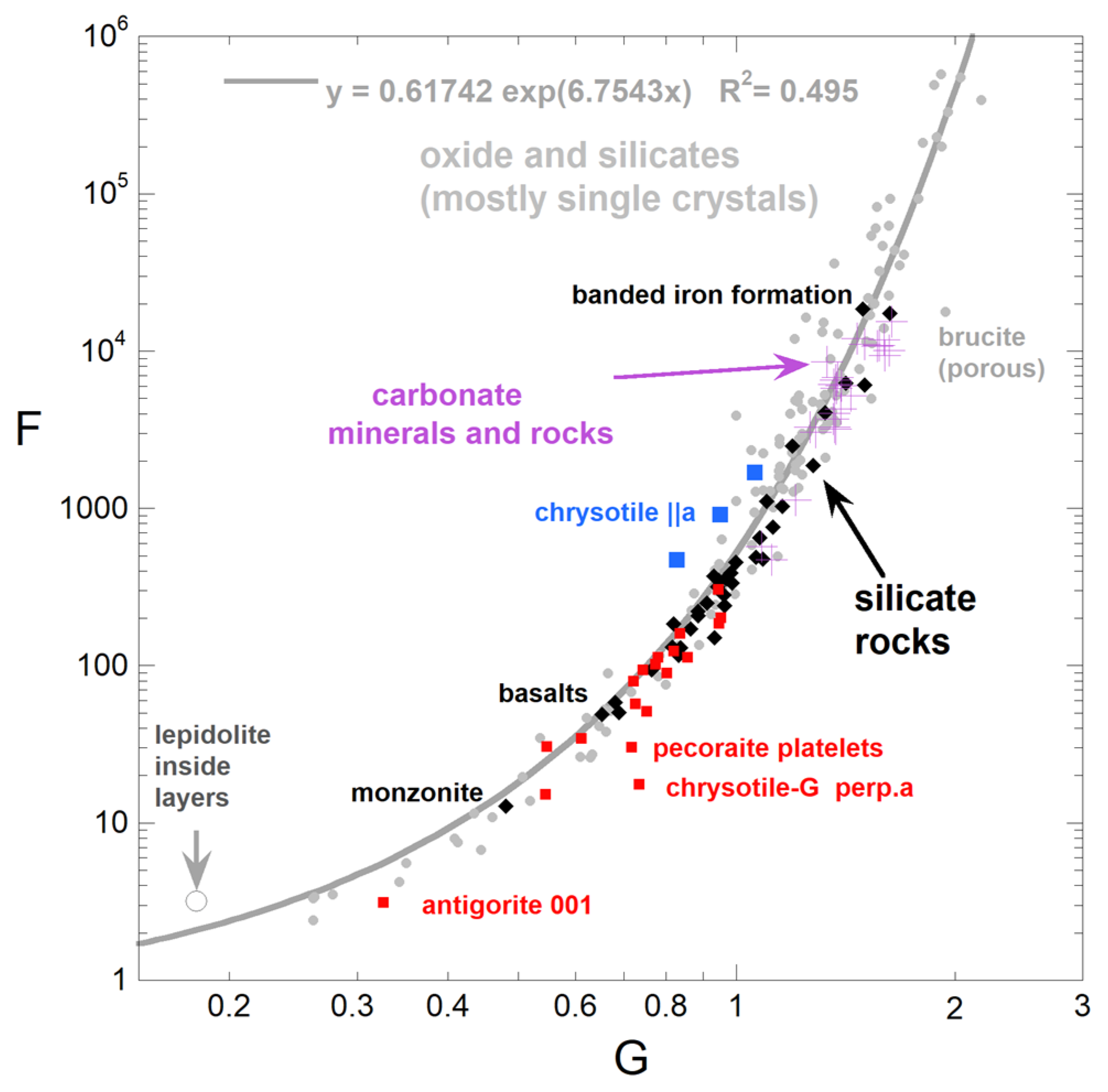
Values of F vary widely, from 3 to 470, mainly because units of F depend on G. The power law parameter-G varies from 0.32 to 0.95, with an average of 0.75 ± 0.15. The high T parameter H varies from ~0 to 0.000044, with an average of 0.00002 ± 0.00001. Values of H are typical of silicate minerals [5] (ch. 7). Parameters F and -G of serpentines are correlated, as observed previously for silicates, carbonates, and oxides (Figure 9). Departures from the fit are associated with minerals for which parameter H is equivocal, due to limited T range or very flat curves (e.g., antigorite 001). Although H is small, it important to obtaining an accurate fit.

4.6.3. Thermal Diffusivity vs. Temperature for Bulk Serpentines

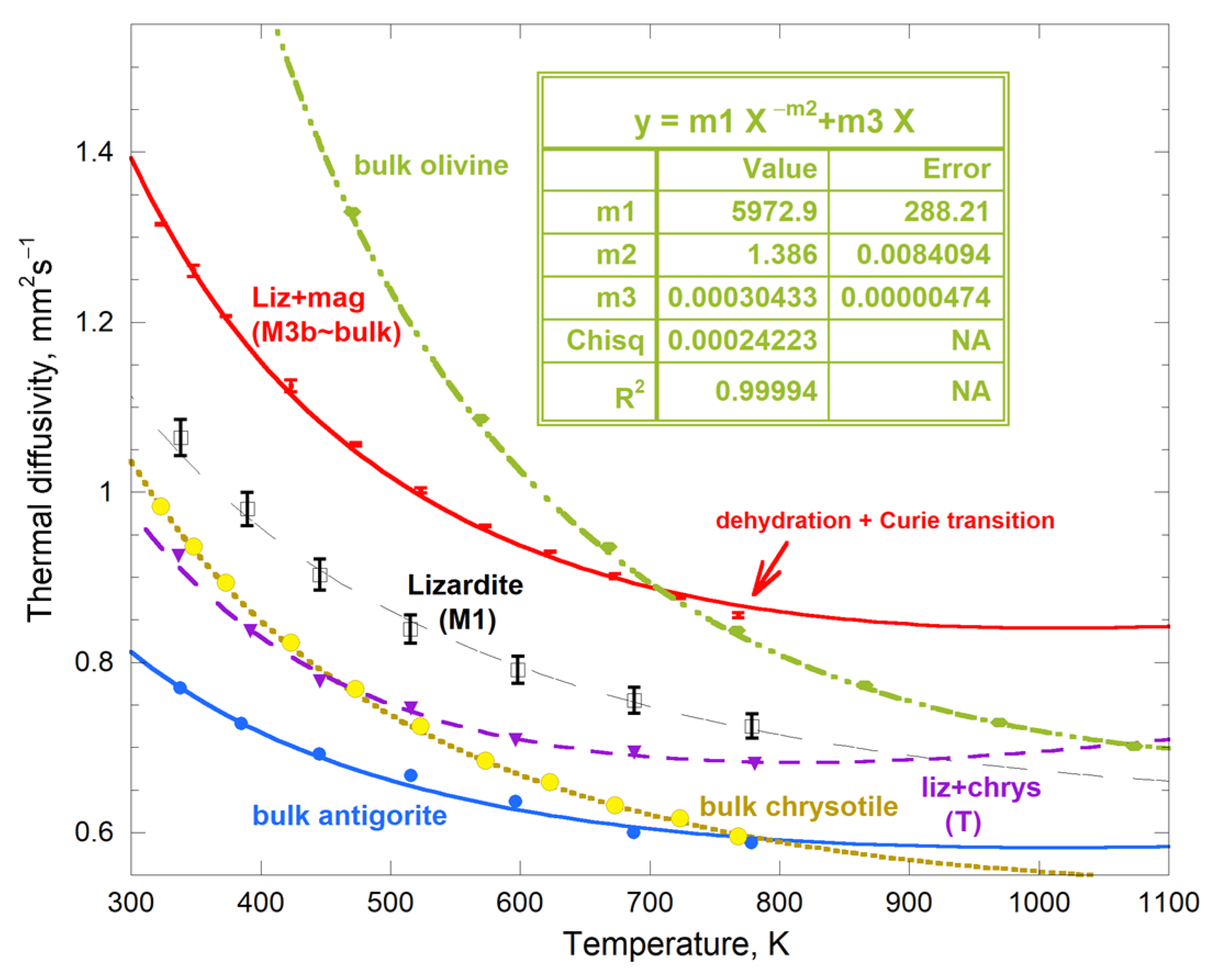
Data on oriented antigorite and chrysotile were averaged according to the RHS of Equation (13) to provide bulk (polycrystalline) mineral values (Table 4; Figure 10). Both samples are near-endmember. Chrysotile has minor magnetite.
Scant orientational differences exist for the three perpendicular cuts from each of Liz-M3 and Al-serpentine. Slight differences in impurities exist (Table 3). On this basis, Liz-M3 section b and Al-liz section a, both with intermediate D values, are proposed to represent bulk properties of near-endmember (with magnetite) and Al-rich lizardites. Other Mg-rich lizardites are shown in Figure 10, for comparison.
Equation (13) represents random orientations of grains in a sample. Chrysotile sections perpendicular to a dominate due to equivalence of the tubule directions. Even so, chrysotile bulk D exceeds that of antigorite at all T (Figure 10). Thermal diffusivity of lizardite is the highest of the three polymorphs.
Figure 10. Thermal diffusivity deduced for randomly oriented crystallites, which depicts bulk D, using the LHS of Equation (13). Least squares fits of Table 4 are shown, plus a new Equation (13) fit for olivine [17], shown as olive ovals and dot-dashed curve. Blue dots = bulk antigorite, calculated from fits to oriented D in Table 4. Tan circles with yellow fill = chrysotile, incorporating the preferred fit of Table 4 for ||a. Purple triangles = liz-T. Open squares with error bars = lizardite M1. Red squares with tiny error bars (LFA-467 runs) = lizardite M with a small amount of magnetite.
Minerals 16 00509 g010

4.6.4. Effects of Impurities on Serpentine Thermal Diffusivity

The Curie transition slightly affects the trends for Liz-S1 and Liz-M3 in Figure 8a, both of which had 3 to 4 wt% Fe3O4 from XRD powder data. Post LFA XRD patterns of lizardites-M1 and -M2 did not indicate magnetite. However, D of M2 decreases towards the Curie transition, suggesting that magnetite is present. It is possible that dehydration began by 750 K in our samples, but unlikely, due to the ~10 min that our samples were at 750 K. Kinetic studies were generally at 775 K and higher and over longer times for all three polymorphs (e.g., [69,70,71]).
Low D for liz-M1 is consistent with this sample being the best representation of pure lizardite (negligible magnetite). Because liz-M3b has high D-values, plus an obvious downturn as the Curie point is approached, this sample best represents lizardite + magnetite.
Our Al-lizardite lacks magnetite, but has brucite impurities. Details are given above.
Many of our lizardites have intermingled chrysotile (liz-T, -S, -G, and -W). Slight differences are attributed to proportions and minor impurities observed in chemical and XRD analysis. Equation (13) was not applied to mineral proportions because the amount of impurities varies between the sections of any given sample. Additionally, impurities of chrysotile are difficult to detect via XRD in low amounts, yet clearly affect thermal diffusivity. Given the similarity of liz-T, -S1, and -G trends, fits for any of these (Table 4) can be used to represent lizardite-chrysotile mixtures.

4.6.5. Effects of Site Substitutions on Serpentine Thermal Diffusivity

Impurities limit quantitatively probing the effect of cation substitution. Nonetheless, it is apparent from the chemical compositions (Table 1 and Table 2) and the data in Table 4 and Figure 8 that substitution of Al increases D substantially at constant Fe (cf. liz-T and Al-liz). Substitution of Fe or Ni decreases thermal diffusivity at constant Al content. This finding is in accordance with the vibrational frequency of Al in the octahedra being higher than Mg and vibrational frequencies of Fe being lower than Mg.

4.6.6. Available LFA Data on Serpentine Rocks

El Alami and Bennouna [12] report rock thermal diffusivity from LFA as ~1 mm2 s−1 at 298 K and ~0.65 mm2 s−1 at 875 K. Neither a graph nor tabulated data were provided and links of D to their three chemically and structurally different serpentinites were not mentioned. Their two reported D-values are close to those from serp-G, which serves as a proxy to calculate serpentinite thermal conductivity below.

5. Thermal Conductivity from LFA Results

5.1. Literature Data on Static Properties

Literature data needed to calculate K(T) from Equation (5) and K(P) from Equation (7) are listed in Table 5. Measurements are limited mostly to low-Fe antigorite and chrysotile. Data sources and brief descriptions of the samples are given in Table 5 notes.
Density was ascertained mostly from previous XRD reports, and represents material with low porosity, roughly below 1%. Porosity effects on chrysotile (tubules are porous) are discussed below.
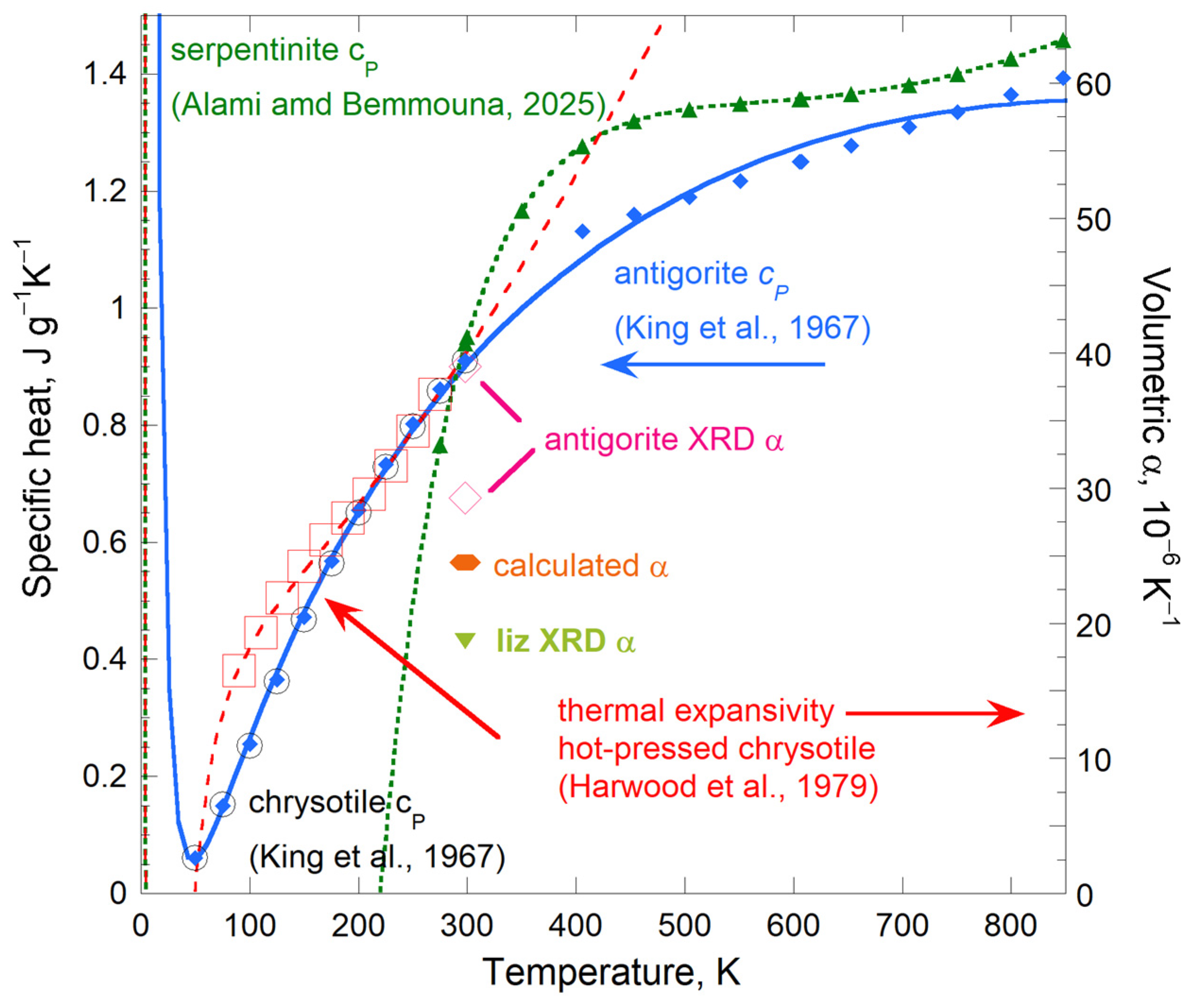
Specific heat data for single phases were obtained below 298 K (Figure 11). Least squares fits of specific heat to a Maier–Kelly form are listed in Table 5. We used the high-T fit obtained using enthalpy data [72] to describe antigorite. Because chrysotile and antigorite cP are nearly identical below 298 K, this should also represent chrysotile. Lizardite cP seems unavailable. Based on reasonable agreement near 298 K of chrysotile and antigorite with lizardite rock data [13], the fit for antigorite is also used to approximate cP for Mg-rich lizardite.
Thermal expansivity is directly measured using interferometry. Data at cryogenic temperatures (Harwood et al. [74]) were fit to a 2nd-order polynomial (see Figure 11). Extrapolating this to high T is reasonable as a steeper and higher trend for αvol than cP vs. T is expected [40]. The cause is solids becoming less rigid as T increases, so applying the same amount of heat to the solid at high and low T is more effective at expanding the solid [40]. Appendix B provides examples.
Measurements of volume (V) vs. T using XRD provide an average αvol = V−1V/∂T over the range of measurements, due the combination of low αvol with uncertainties in bond lengths providing only a linear dependence of V on T. Disagreements at 298 K (Figure 11, Table 5) are typical of silicate minerals; see, e.g., the compilation of Fei [79]. To provide an additional constraint, Section 5.2 calculates αvol from elasticity data.
Bulk moduli are mostly ascertained from V vs. P also using XRD [75,76,77]. The linear dependence of V on P likewise provides average compressibility = B−1 = V−1V/∂P over the range of measurements. Because B increases with P, this result is higher than B at 1 atm, and so an equation-of-state is used to provide the values listed in Table 5. Assuming a value for B’ = ∂B/∂P is required. Typically B’ = 4 is used.
Elasticity measurements of single-crystal antigorite using Brillouin scattering provide adiabatic B = 68.5 GPa and shear modulus G = 38.5 Gpa for bulk values for the Voight–Ruess–Hill average (Bezacier et al. [80]). Theoretical considerations indicate that volumetric and elastic determinations probe the same bulk modulus, which equality holds within experimental uncertainty for hundreds of substances at ambient conditions and for dozens of metals and insulators that are well-studied at high T [40]. One reason is that constant temperature results from keeping the heat input from the surroundings constant. Brillouin scattering [80] results are compatible with assuming B’ = 4 to evaluate XRD data (Table 5).
Ultrasonic measurements [81] provided much lower B compared to all other measurements. Sample density is low, 2560 kg m−3, suggesting that porosity is the source of the discrepancy with [80].
From XRD data, Yang et al. [76] provides ∂B/∂T = −0.026(4) GPa K−1. Equation (7) then yields δT = 9.7, which is large compared to the typical value of 7 from better constrained elastic data [39]. Given uncertainties in ascertaining derivatives from volumetric measurements, we use δT = 7.

5.2. Additional Constraints on Thermal Expansivity

Applied heat performs work which expands the solid. The relevant formula for an isotropic substance is
α v o l = const . ρ c P Υ   where   Υ = 3 B G 4 B + G   and   const . 1 ,
where Υ = Young’s rigidity modulus [40]. Appendix B provides mineralogical examples.
For single-crystal antigorite, Brillouin scattering [80] gives Young’s modulus Υ = 97.3 GPa. Equation (16) then gives αvol = 2.45 × 10⁻⁵ K−1 at 298 K.
All three structures have similar ρ and B at 298 K. Antigorite and chrysotile have nearly identical cP, so lizardite cP should not differ appreciably. On this basis, Equation (16) suggests that αvol values should likewise be similar. Averaging our calculation with the four experimental values (Table 5) provides 3.1 × 10⁻⁵ K−1, which is typical of minerals at 298 K (e.g., [79]).

5.3. Thermal Conductivity vs. Temperature Calculated from Thermal Diffusivity

Equation (5) for K requires D, ρ, and cP. For bulk samples, Equation (13) is used, which is analogous to the Voigt–Reuss–Hill average of elastic constants. Calculations are separately made at ambient and elevated temperature, respectively, using direct measurements and curve fits.
Ambient density is accurately known for all three polymorphs (Table 5). Adiabatic measurements with uncertainties of ±½% provide identical cP below 298 K for antigorite and chrysotile [72]. This value (Table 5) should hold for lizardite, which basically is composed of small domains of the other polymorphs, as well as for lizardite-chrysotile mixtures. On this basis, K(T = 298 K) (Table 6) is accurate to better than ±4% for all mineral phases listed. The serpentinite rock K has less accuracy due to use of digital scanning calorimetry data (~±3%) and the approximate D(298) from [13].
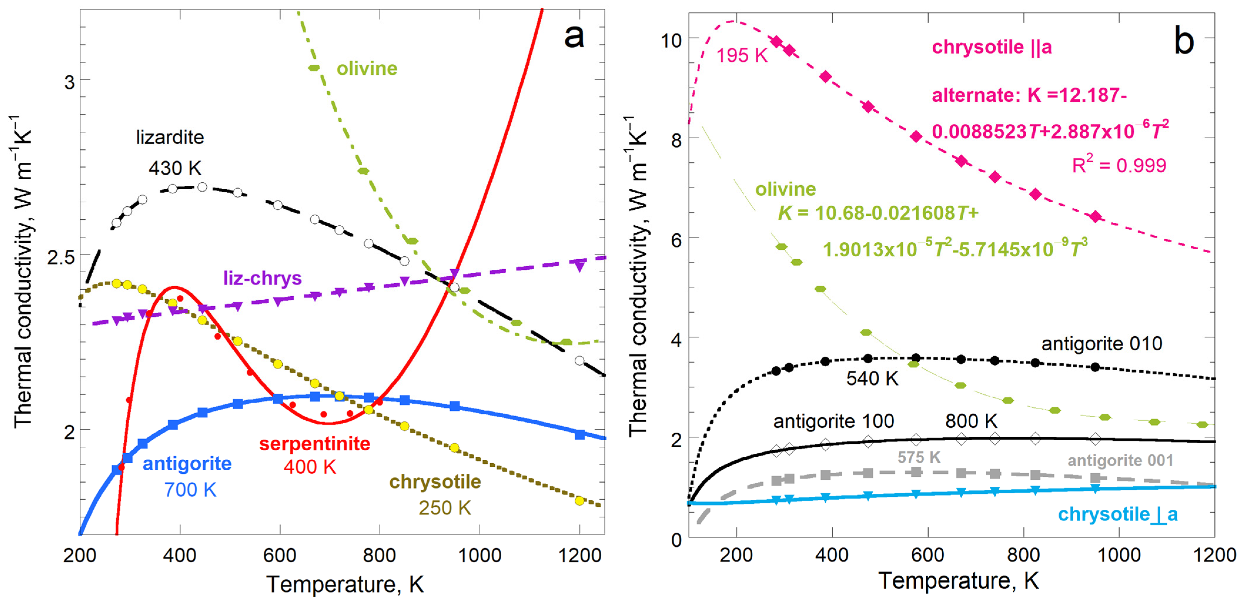
Calculations are less accurate at high T because limited data exist for both V(T) and cP(T). Serpentine phases have low αvol and thus ρ slowly changes with T (Section 5.2; Figure A1). In contrast, cP (Figure 11) increases substantially with T above 298 K, which contrasts with D which mostly decreases weakly with T (Figure 8). Due to different behaviors and larger uncertainty in cP at high T, constant density is used to calculate K(T) from Equation (5). For the bulk samples, the fit to cP for antigorite (Table 5) is combined with D(T) for Liz-M1, or with bulk D(T) for each of antigorite and chrysotile, or with liz-T for mixed serpentine phases (Table 4). For serpentinite rock. we combine its cP (Table 5) with D(T) for serp-G (see Section 4.5). Results are shown in Figure 12 with fits in Table 6. A slightly modified Maier–Kelly form, which reproduced K(T) for basaltic glasses and lavas [37], well describes K(T) of serpentines due to changes in cP likewise exceeding those in D as T increases (cf. Figure 8 and Figure 11).
Ambient K is low for serpentines, except for chrysotile ||a (along the tubules. Thermal conductivity reported for chrysotile should be reduced by a factor of 0.85 to account for porosity on density in Equation (5), see Table 6 footnotes. This deduction is supported by comparison to cryogenic measurements of [10] (Section 6.2.2).
The curves for K vs. T show various behaviors. Trends calculated with well-constrained inputs to Equation (5), namely antigorite and lizardite, are similar, whether presented as bulk or oriented forms. These nearly-pure, single phases have a peaks in K(T) above room temperature. Chrysotile ⊥a and liz-chrysotile have flatter trends so if a peak exists it is above their stability range. Serpentinite behaving differently is attributed to specific heat and thermal diffusivity being measured on different samples. Even so, serpentinite also shows a peak in K above ambient T and fairly constant K up to dehydration near 850 K. Section 5.3 continues discussion of the various trends.
Figure 12. Thermal conductivity vs. temperature. Serpentine fits for D and cP from Table 4 and Table 5 were extrapolated above 850 K. Samples are as labelled. Temperatures indicate the position of the maximum in K(T), if present. Symbols show every 4th point calculated from Equation (3), where data on D were extrapolated to 273.15 K. Curves are least squares fits of Table 6. (a) Bulk samples, based on D from Equation (13). Serpentinite is the only phase where cP data of [13] were used. Olivine K obtained from LFA on single crystals [17]. (b) Oriented samples, based on directly measured D(T). Examples of fits are shown.
Minerals 16 00509 g012

5.4. Thermal Conductivity vs. Pressure Calculated from Fourier’s Law

Integrating Equation (7) gives the pressure response at ambient temperature:
K ( P ) = K 0 1 + B B 0 P 7.33 B ,
where K0 = K(298), listed in Table 6. For the combined P, T response, K0 is replaced by the fits for K(T). Because the term BP/B0 is small, the following linear approximation to Equation (17) holds up to P~25 GPa for these lithospheric phases:
K ( P ) K 0 1 + 7.33 B 0 P   or   K ( 298 ) P 0 7.33 K 0 B 0 .
Knowledge of ∂B/∂P, which is unconstrained, is unnecessary. However, bulk modulus from XRD is uncertain and dependent on the choice of B′. Hence, we use an average B0 = 64 ± 2 GPa to provide the initial slopes ∂K/∂P listed in Table 6. Given the uncertainties, and lack of information, effects of orientational differences for B on Equation (18) are not considered here. These should be slight, except for chrysotile.
Alternatively, the initial pressure response can be represented as ∂(lnK)/∂P, which equals ∂(lnD)/∂P (Equation (9)). The value is 11 ± 1% GPa−1 for B0 = 64 ± 2 GPa. Serpentines are compressible. For comparison, much stiffer olivine with B of 128 GPa has ∂(lnK)/∂P near 4% from experiment and 5.5% from theory [27,38]. Bulk moduli of a material controls the response of its thermal conductivity to pressure because energy (i.e., light or heat) does not compress.

6. Discussion

6.1. Implications of Spectral Data

6.1.1. Site Speciation and Charge of Transition Metal Ions in Serpentines

Serpentines are generally close to the Mg endmember, but low amounts of Fe are not amenable to accurate Mossbauer analysis [82,83]. These studies, on serpentines with FeO averaging 3–4 wt% FeO, show that the ratio Fe3+/Fetot varies widely, from 0.2 to 0.85, with an average of 0.5; ratios from Xanes method are systematically higher [82,83]. In our Fe-poor suite (averaging 1.7 wt% FeO: Table 3), visible spectra show that Fe3+ dominates Fe2+, where the latter is commonly negligible. Exceptions are antigorite and Thetford chrysotile with very low Fe, in which cases, all iron is Fe2+. Because Globe chrysotile has entirely Fe3+, we suggest that the bimodal speciation results from very low Fe content and the need to conserve charge, not the structural polytype.
We also find that the amount of Cr3+ incorporated affects Fe site speciation, which was not noticed previously, since Cr3+ is not detectable by Mossbauer. Cross relaxation between Fe3+ and Cr3+ was observed in a Mossbauer study of other materials [84].
Our study also documents the first detection of Cr3+ occurring naturally in octahedral sites of a mineral. This finding may be connected with the high concentrations of Cr in pecoraite, suggesting that other minerals with large amounts of Cr and Ni may also have this unusual crystal chemistry.

6.1.2. Symmetry Analysis and the Number of O-H Peaks

For the ideal structures, symmetry analysis suggests that two O-H stretching modes should exist parallel to the c-axis and that four M-O-H bending modes are expected perpendicular to the c-axis [66]. Flat sections of fibrous chrysotile provide both orientations. The spectra (Figure 7b) show three O-H stretching modes (and three stretching overtones). Excess bending modes are also observed.
Additional OH bands support our proposal of a charge-coupled substitution (Equation (15); Figure 4) providing excess OH. Two additional reasons exist: (1) Chrysotile from Thetford with tiny amounts of Al (Table 1) lacks excess OH. (2) All three polymorphs have the number of H bands exceeding the number expected plus the spectral patterns are similar in the three polymorphs.
Even so, Equation (15) needs further evaluation, given experimental uncertainties of ~±2% in EPMA [49]. Also, EPMA data on soft minerals may be affected by imperfect polish.

6.1.3. Inference of Ballistic Transport Conditions from IR–Visible Spectra

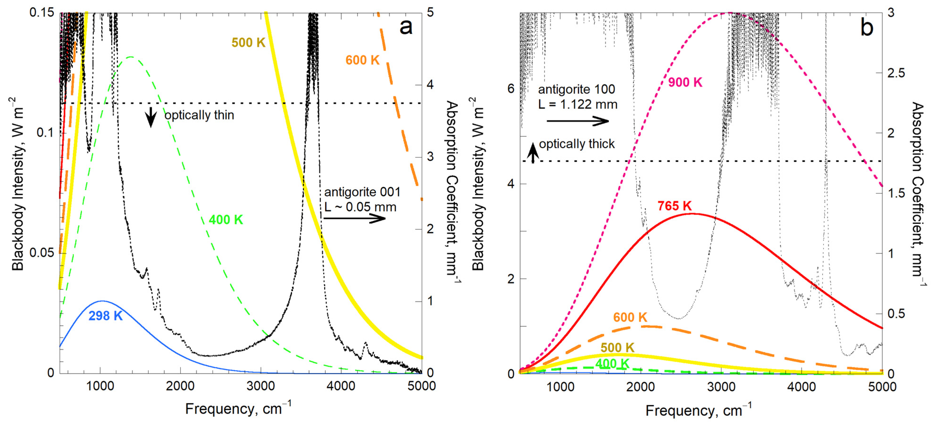
Infrared fundamentals occurring at ν < 1000 cm−1 have extremely large A, requiring sample thickness <1 μm for quantitative spectroscopic study [66]. Thicknesses of ~1 mm used in LFA transmit negligible light for ν < 1900 cm−1 (Figure 6 and Figure 7a). Thus, infrared fundamentals and the lower frequency overtones diffuse heat in our experiments.
Overtones and combination bands exist above 1000 cm−1. Serpentines partially transmit light between ~1900 and 2800 cm−1, so ballistic transport exists in the higher frequency near-IR (overtone) region even near 298 K (Figure 13a). As T increases, the blackbody curve shifts toward the visible region (Figure 13b), and so ballistic transport increases with T. By ~800 K, substantial ballistic transport occurs above 5000 cm−1 (Figure 13b) and into the visible for weakly colored serpentines (Figure 6 and Figure 7b). Small amounts of ballistic transport are evident in the raw LFA data of our serpentines, namely the time-temperature curves, and were removed by modelling [34].
Strong absorbance near 3000 to 3600 cm−1 (the O-H stretching region) could contribute to diffusive heat transport above ~800 K. However, at ambient pressure, serpentine dehydrates above ~800 K, so the participation of O-H modes in heat transfer of serpentines appears unimportant.
Figure 13. Blackbody intensity (flux, in various colors, as labelled, on the left y-axis) compared to unpolarized infrared spectra of antigorite (black or grey curves and the right y-axis). No relationship exists between the left and right y-scales. (a) Low temperature flux compared to the 001 face. Thickness was not verified, so absorption coefficients may be a factor of 2 higher than actual. “Optically thin” is defined by noise in the spectra. (b) Flux for temperatures of LFA runs compared to the verified A for 100 face. By 700 K, the peak of the flux lies in the transparent region between the lattice overtones and the main O-H stretch. The 100 face is shown because D from this face is close to the average of the three orientations.
Minerals 16 00509 g013

6.2. Comparison with Previous Heat Transport Studies of Serpentines

As shown below, quantifying heat transport properties for serpentine minerals and rocks via contact methods is greatly impeded by thermal contact losses, ballistic radiative transport gains, and deformation during compression. Pale colors and low rigidity of serpentines are sources of these systematic experimental errors. Previous studies are discussed individually.

6.2.1. Previous LFA Measurements of Serpentine Rocks

Approximate values of D at 298 and 875 K from LFA reported by El Alami and Bennouna [13] for three serpentinites are consistent with D(T) for our serpentines, permitting calculation of K(T) for serpentinite rock (Table 6). However, K(T) is uncertain (~±7%) between ~350 and ~800 K and the trends cannot be extrapolated with confidence.

6.2.2. Cryogenic Study of Chrysotile Parallel to the Tubules

Kumzerov et al. [10] applied the steady-state contact method of [85] to chrysotile tubules along the a-axis. Samples have 5%–6% porosity. Bulk sample size was 5.5 mm × 6.5 mm × 12 mm. Thermal conductivity having a peak is observed for all solids and expected from spectroscopic modelling [5,29]. At the maximum T reached (~298 K), K of chrysotile parallel to a is 6.5 W m−1 K−1.
For K ||a, LFA suggests a higher T for the peak (195 K) than the Ref. [10] maximum at 150 K. The difference is connected with extrapolation of higher T data, so agreement is reasonable. LFA provides significantly higher K at 298 K (Table 6). This difference is due to (1) contact losses, especially as steady-state techniques require two contacts and losses are typically 10% per contact [14,15]. Another contribution is use of crystallographic density in our computation, which overestimates our K. Lower density of 2190 kg m−3 [58] accounts for the remaining 20% discrepancy.
  • To account for porosity of tubules, K-values in Table 6 for chrysotile should be multiplied by 0.85 = 2190/2570.

6.2.3. Long-Cylinder Contact Method Applied to Lizardite Rocks

Seipold and Schilling [11] applied the method of Seipold [86] to fine-grained serpentine rocks. Ballistic radiative effects are present, as demonstrated by comparing the raw data collected by Seipold [83] to the theoretical curves of Cowan [87], and by K increasing with T at very low T (300 K) for some samples.
Thermal conductivity values for most of their serpentinites oscillate with temperature [80]. This strange behavior is attributed to use of 3 s pulses [11,86] when heat crosses 1 to 3 mm thick rocks with diverse mineralogy within 1 s, as shown by LFA experiments [42,68]. Given the many problems with Seipold’s [86] technique, that mineral compositions were not provided, and that the reported pressure coefficient of ∂(lnK)/∂P = 14.8 ± 6% GPa−1 [83] is highly uncertain, despite being the average of several measurements, these studies do not provide useful information.

6.2.4. Needle Point Method on Antigorite Powder

Antigorite K(298) obtained from a dissolved sample using the needle point method [6] is ~50% larger than the bulk result of Table 6. The composition was not reported and this technique is known to be highly uncertain (e.g., [5]).

6.2.5. Modified Angstrom’s Method on an Antigorite Polycrystal

Osako et al. [8] studied polycrystalline antigorite at high pressure using a periodic technique. Density of 2585 kg m−3 suggests porosity near 2%. Total thickness of the two sample layers is ~1 mm. The reported Fe/(Mg+Fe) ratio of 0.007 is lower than the antigorite studied by spectroscopy here, so ballistic effects are expected. Standards were not measured so experimental uncertainty is unconstrained. The geometry provides two-dimensional heat flow, which is neglected in their modelling, but would artificially elevate K for the geometry used [8].
As preferential compression of pores and deformation of these soft samples is expected at very high pressure, discussion is limited to the initial trends in P. These are K = 2.4 + 0.07P in Wm−1K−1 and D = 0.91 + 0.007P in mm2s−1, where P is in GPa [7]. Derivatives are thus 2.9% Gpa−1 for K and 0.8% Gpa−1 for D, which are incompatible with theory (11 ± 1% Gpa−1 for both). Ambient values from [8] are 25% and 12% higher than LFA data on bulk antigorite (1.92 Wm−1K−1 and 0.81 mm2s−1). Inferred specific heat is 10% higher than calorimetry data [69]. These differences are outside the uncertainties of measurements and theoretical calculations.
Earlier results for olivine [88], obtained using the same method, provided D higher by 10 to 23% for the three orientations at room temperature than LFA data, which probed the same composition (93 mole % forsterite) [17]. Spurious radiative transfer is evident in olivine data from [85] along the b-axis above 700 K, as shown in [14] (their Figure 10). The pressure derivative of 3.5 ± 0.5% GPa−1 for olivine [82], which has high bulk modulus (~110 GPa, providing 4.9% GPa−1 from Equation (17)), is reasonable but slightly low.
Two-dimensional heat flow best explains the consistently high values of K and D associated with this technique in [8,85]. Pressure derivatives for antigorite being especially low are compatible with deformation, based on antigorite being considerably weaker than olivine. Deformation uptakes applied heat. Transport is impeded, and so the pressure derivatives of K are too low.

6.2.6. Thermoreflectance at Pressure of Thin Antigorite

Chien et al. [9] studied antigorite slabs at 298 K with ~30 μm thickness coated with Al in a diamond anvil cell with a silicon oil pressure medium. The Fe/(Mg + Fe) ratio of 0.0167 is close to our antigorite (0.0175). Density was not reported.
From their first figure of [9], the 010 face has K = 4.6 Wm−1 K−1 whereas the 001 face has 1.05 Wm−1 K−1. The 001 face is close to our result (1.17 ± 0.04 Wm−1 K−1). The 010 face is 34% higher than our result of 3.43 ± 0.10 Wm−1 K−1. This large discrepancy is attributed to multiple free parameters used in thermoreflectance and the need for a similar standard.
Initial slopes from the first figure in [9] are both 0.29 Wm−1 K−1 GPa−1, but this equality is unexpected per our analysis of Fourier’s laws (Section 2.2.1). For 010, their graph provides 6.3% GPa−1, and for 001, the slope is 27% GPa−1. The orientation difference in P derivatives requires substantial variation in directional bulk modulus from the bulk value of ~64 GPA, which provides 11 ± 1% GPa−1. Derivatives from [9] suggest B = 112 GPa for 010 and = 26 Gpa for 001 directions. This spread seems inconsistent with measured sound speed variations [80,81].
Thermoreflectance at best attains the nominal uncertainty of ±5% [18]. Comparing such results for antigorite [9] to LFA data on a similar composition show that the accuracy is worse than previously inferred. Importantly, samples used in thermoreflectance are very thin and should provide values much lower than measurements on macroscopic, mm sized samples per theory and experiment (Section 2.1.1). Values resembling macroscopic data are a consequence of thermoreflectance utilizing multiple free parameters and resting on comparisons with previous studies.
Deformation of the thin plates is possible. Perhaps this explains the peculiar high-P maximum shown by [9]. Lastly, physical contacts in thermoreflectance studies should provide losses, so K-values should be less than those obtain in LFA (Table 6).

6.2.7. Antigorite Rock at High T and P

Wei et al. [11] studied an antigorite-carbonate-magnetite rock up to T = 1300 K and at P = 0.5, 1 and 2 GPa. Mineral proportions (65% serpentine) from point counting differ from 75 to 78 wt% serpentine suggested from normative analysis of their reported whole rock chemical composition, which had 34.2 wt% SiO2, and should represent the bulk sample rather than the surface, as is explored in point counting.
The technique is denoted as transient plane wave, but is actually periodic. The configuration indicates that heat flow is two-dimensional, which was not modelled, and would provide higher D and K than is inherent to the phase. A standard was not measured, so uncertainties are unconstrained. Optimistic uncertainties of ±5% for K and D [1], coupled with losses at contacts, make extraction of heat capacity (Equation (3)) uncertain by ~10 to 40%.
Derivatives are reported in [11] as 5.1% Gpa−1 for K and 11.7% Gpa−1 for D. The latter is compatible with theory for antigorite (11% Gpa−1 for both D and K). However, magnetite and calcite have higher B of ~200 and ~130 GPa, respectively, depending on composition and technique. So reported ∂(lnD)/∂P is actually higher than expected for such rocks, while reported ∂(lnK)/∂P is lower. Deformation occurs, as shown in [11] (their Figure S4).
Reported ambient values of 3.1 Wm−1 K−1 and 1.23 mm2 s−1 [11] seem high compared to bulk antigorite with 1.92 Wm−1 K−1 and 0.81 mm2 s−1 at 298 K. However, calcite and magnetite would elevate rock transport values, and so Wei et al.’s [11] ambient values are reasonable, if the rock has 65% antigorite, but are too high for ~76% suggested by normative analysis.
Spurious, ballistic effects are obvious by 900 K. The data were inappropriately fit with a T3 term, for which usage was incorrectly attributed to our papers on radiative transfer (e.g., [21]), where the opposite was stated. See the introduction, Section 2.1.1 and [5,16,17]. Consequently, values at elevated T from [11] are problematic, and so their models of slab temperatures significantly err.

6.3. General Response of Heat Transport Properties of Silicates to Elevated T and P

6.3.1. Temperature Effects

Our previous work provided a simple formula (Equation (10)) for D(T) and showed that the slope ∂D/∂T becomes flatter as D(298) decreases [41]. This is evident in the power G depending on the prefactor F in Equation (10), as shown in Figure 9. Serpentines behave likewise (Figure 8, Figure 9 and Figure 10).
Thermal conductivity vs. T depends on the product of D with cP, since density changes very little with T. Specific heat ranges from 0 at the limit of 0 K to about 1 J g−1 K−1 near 800 K for minerals, rocks, and glasses (e.g., Figure 11; see also [37]). Hence, substances with high D(298) have comparatively high K(298) and a steep decrease to a flat trend (e.g., olivine and chrysotile||a in Figure 12). Substances with low D(298) have flat trends that are controlled by the increase in cP (e.g., chrysotile ⊥a and antigorite 001 in Figure 12; feldspar minerals shown in [5] (pp. 197–198); and mid-ocean ridge basalt (MORB) glass data are shown in [37]). (Note: the fits in [5] used a simple average for D as this work predates Equation (13).) Behavior at intermediate D(298) is more variable, which is connected with (1) tradeoffs of F and G with parameter H in Equation (10), which describes the high-T trend of D, and (2) with variations in the shape of cP with T (e.g., Figure 11). The complex trend of K(T) for serpentinite closely resembles that of MORB lavas [37].
Consequently, three different fitting forms are used to describe K vs. T. The forms largely depend on D(298) but not entirely (Figure 12). Specifically,
  • For with high D(298), a power law describes K(T). This can be extrapolated only to modestly lower temperatures, as a peak exists at cryogenic temperatures.
  • For very low D(298), a 2nd order polynomial or sometimes a linear fit suffices, because a peak in K(T) is either very broad or at very high T. A modified Meier–Kelly form (Table 6) also fits the data:
K ( T ) = a + b T + c T 2 + d T 1 2 .
  • At intermediate D(298), Equation (19) fits K(T) better than a high order polynomial. Equation (19) has the advantage of extrapolating well below 298 K, which feature includes materials with low D(298). This form fits data on mid-ocean ridge glasses and basalts [38] up to melting at 1450 K.
Our results for serpentines confirm that the peak in K(T) is due to the contrasting responses of D and cP to T, as discussed in many of our papers. We further show here that inefficient thermal conductors (serpentine minerals) have peaks well above room temperature (Figure 12). The peak is not relegated to cryogenic temperatures as is commonly assumed (e.g., [10]) nor is due to a change in scattering mechanisms (Umklapp vs. normal) as in phonon-scattering models [5]. These older ideas are based on data for simple materials with very high D(298). The peak in K(T) occurs in diffusive radiative transfer models that approximate absorption over infrared frequencies as a boxcar function or ramp, with a single parameter [5,29].

6.3.2. Pressure Effects

Response of transport properties to pressure is simple because population of energy levels is unchanged with P. Behavior upon compression is harmonic. Fourier’s law provides an identity for the dependence of D or K on P, which is linearized in Equation (18).
Data on K or D vs. P of stiff materials adhere to theory [27], but not serpentine, which is compliant. Fourier’s law assumes that deformation is not occurring. The low bulk modulus and grainy nature of serpentines is conducive to deformation. Hence, the experimental data record effects distortion, not intrinsic changes in thermal transport (Section 6.2). Compression studies are uniaxial to some degree and also decrease the thickness (aspect ratio) as well as the volume, which changes are rarely discussed.

6.4. Implications for Slab Behavior

Previous thermal models of serpentized slabs are based on inaccurate transport data on either nearly pure antigorite or poorly characterized rocks (Section 6.2). Since our results differ significantly in regards to ambient transport properties plus their P and T derivatives, the deductions of [8,9,11,12] are questionable, if not invalid.
As discussed in Section 5, additional data on specific heat and thermal expansivity are needed for an exacting description of K and thus of the thermal state of subducting slabs. Stability relationships are ascertained using cP (e.g., Evans [1]), but data do not exist for pure lizardite. Results on heat transport properties suggest the following dynamic behavior:
Based on abundance, lizardite is taken as the relevant polymorph. Olivine is considered to be the dominant mineral in the upper mantle and deep slabs. Figure 12 shows that thermal conductivity of olivine (from [17]) drops below that of lizardite at the decomposition temperature at ambient pressure. Enstatite has lower D and K [89], so this crossover in efficiency of heat transport would occur at a lower temperature than the simple end-member decomposition described in Equations (1) and (2). Magnetite has high D (Figure 8d) so allowing for its presence also moves the crossover in K to higher T. Importantly, the univariant phase boundary moves to higher T as pressure increases, but the pressure dependence of this boundary is low (flat) [2] (p. 201). Thus, temperature effects are most important to slab behavior. From data on K and D, warming of the slabs is enhanced by the presence of lizardite, which drives their temperature to the decomposition phase boundary.
Pressure enhances K of lizardite at double the rate of olivine. Enstatite with B ~110 GPa has low ∂(lnK)/∂P of ~7% GPa−1. Magnetite has a high B > 180 GPa so changes little with P, being <4% GPa−1. These less abundant phases reduce the difference between serpentized regions and mantle harzburgite, but the serpentized regions would still have higher K due to compression. As slabs sink, the presence of serpentine drives the slab towards higher temperature and towards the univariant phase boundary.
During decomposition, H2O is released. As slab temperatures substantially exceed 400 K, the state of H2O is vapor, which has extremely low density, and so would rise through the slab and overlying mantle. Rising steam carries heat away, and thus decomposition drives the slab to the univariant phase boundary, but in the opposite direction as simple warming or compression.
For the above reasons, conditions in subducting, serpentized slabs should lie on the decomposition phase boundary. Buffering along univariant phase boundaries has been connected with production of large volumes of basaltic melt [37]. Thermoregulation appears to be important to the thermal state of planets [90].

6.5. Future Work

Scant data on specific heat has prevented generalization of our measurements to mineral compositions beyond those probed here and the development of quantitative thermal models of slabs. Measurements of cP for lizardite, the most common phase, and its mixtures with the other polymorphs are particularly needed. Although cP of antigorite and chrysotile nearly match below 298 K, this need not be true of lizardite. However, the more likely departure from antigorite cP is that of mixtures. Disorder is known to lower cP.
Although density of silicates changes little with T, accuracy in K at high T would be improved through additional measurements of thermal expansivity. Crystallographic studies are insufficiently accurate to ascertain the ubiquitously low values of α, as shown by discrepancies in Figure 11, and in the tabulations of [79] for many minerals. More accurate, direct measurements of α attainable via dilatometry and interferometry are needed. This is true for minerals in general and serpentines in particular.
Elasticity studies likewise need revisiting. Again, the most common polymorph, lizardite, has not been studied, other than by crystallography. This phase behaves as if isotropic, so bulk properties could be obtained with relative ease on homogenous appearing lizardites (e.g., liz-M).
Such data, combined with available measurements of the common impurity phase (magnetite) in a mixing model Equation (13), would yield more accurate values of K and D than are possible with conventional contact methods and problematic thermoreflectance studies.

7. Conclusions

Heat transport remains poorly understood in Earth science due to long-standing reliance on contact methods with known systematic errors. More recent use of thermoreflectance in diamond anvil cell studies likewise involves contact losses and has exacerbated the problem, as results from this model-dependent method are largely unconstrained. As shown here and in our recent study of MORB glasses [37], thermoreflectance provides unphysical pressure derivatives and only yields reasonable ambient values of K by incorporating pre-existing measurements. Such benchmarking is against material that is far thicker than used in thermoreflectance. Thin-film samples have substantially smaller transport properties than macroscopic samples when an absolute technique is used [28].
The present paper makes inroads into quantifying the thermal transport properties of serpentine minerals, particularly the common polymorph, lizardite, with a relevant low Fe composition. Amounts of chromium are shown to be important to site speciation and spectroscopic evidence is presented for additional stoichiometric OH at a site not previously noted in crystallographic studies. The present study advances knowledge of both microscopic and macroscopic behavior of serpentine minerals.
Lastly, new data on the effects of temperature and pressure on lizardite transport properties require that conditions in subducting slabs are buffered to the univariant phase boundary describing decomposition. This finding extends to rocks, but quantification of the depths involved requires additional data on specific heat as a function of temperature of serpentized slabs, or at least on lizardite-chrysotile mixtures. Pressure changes in cP are constrained by a thermodynamic identity [40] that is based on applied heat doing work to expand the solid. Models use an older formula, which describes changes in cp with P as temperature effects. This depiction is not physically sensible, as changes in diverse physical properties with P are regulated by the compressibility of the material, not by its thermal expansivity.

Funding

This research received no external funding.

Data Availability Statement

The original contributions presented in this study are included in the article. Further inquiries can be directed to the corresponding author.

Acknowledgments

I thank P. Carpenter (WU) for considerable help with XRD analysis and electron microprobe data.

Conflicts of Interest

The author declares no conflicts of interest.

Abbreviations

The following abbreviations are used in this manuscript:
LFALaser flash analysis
RHSRight-hand side
LHSLeft-hand side
MORBMid-ocean ridge basalt

Appendix A. Reference Optical Spectra and Band Assignments

Appendix A.1. Previous Optical Spectra of Lizardites

Because absorptions originate locally, i.e., in the cation sites, and structural differences reflect larger length-scales, bands in antigorite and chrysotile spectra can be assigned based on available lizardite spectra. Data are summarized as follows:
Visible–UV spectra of Fe-rich lizardite from the New Caledonia ophiolite show an intense broad doublet at 915 and 1150 nm with shoulders at 645 and 750 nm, assigned to octahedral Fe2+ [59]. This expression is similar to that of many minerals, see, e.g., [60]. Their formulae, Mg2.8Fe0.2Si2O5(OH)4, neglected 0.42 wt% Al2O3 and 0.08 wt % Cr as metal. Their analysis had 37 wt% SiO2, which is lower than expected, and a low total since 18.2 wt%, not ~14 wt% as is typical [2], was assumed for H2O.
The presence of Fe3+ in New Caledonia lizardite is demonstrated by narrow bands at 345, 390, 420, 440, and 460 nm [59]. This pattern partly matches peaks at 380, 420, and 440 nm for tetrahedral ferric iron (Fe3+-tet) in feldspar [61] and glasses [62]. Spectral features of Fe3+ in an octahedral site (Fe3+-oct) are much weaker and difficult to detect [62]. The New Caledonia lizardite has 5.43 wt% Fe as metal, which exceeds the 2 wt% mean of the statistical database [82], and so Fe3+-oct is expected. Spectra of corundum with 0.4 wt% Fe3+-oct have a strong band at 450 nm, a strong double at 390+376 nm and a very strong band at 344 nm [63]. We assign the 420 and 440 nm bands in lizardite to Fe3+-tet, 344 and 460 nm bands to Fe3+-oct and the 390 nm band to both sites.
Spectra of Ni2+ in lizardite show three strong features: a doublet at 400 nm, overlapping bands at 660 and 720 nm, and a broad band at 1100 nm [59]. The presence of Fe2+-oct in mixed Fe-Ni lizardites is best evidenced by a strong band at 910 nm, since the others overlap. The band at 400 nm, which is broader than the spin-forbidden transitions of Fe3+ in either site, and a band at 660 nm, indicates Ni2+ [59].

Appendix A.2. Optical Spectra of Cr3+ in Octahedral and Tetrahedral Sites

Variable amounts of Cr have been detected in diverse serpentines [2] and in our samples (Table 2). However, spectra of Cr in serpentines seem unavailable.
Chromium strongly prefers octahedral coordination. The spectral signature of Cr3+-oct consists of strong, well-separated bands at 450 and 650 nm, as exemplified by tremolite [60] and diopside [24]. Importantly, Cr3+-oct absorbs much more strongly than Fe cations, overriding Fe features in many minerals [60]. The 460 nm band of Fe3+-oct is thus not a useful indicator when Cr3+-oct is present.
The presence of Cr3+-tet in minerals has been debated. However, spectra of synthetic diopsides show that Cr3+-tet has a strong band at 600 nm, which is accompanied by weaker bands at 310, 730, 850, and 1100 nm [24]. This pattern is distinct from those of Cr3+-oct [60] and of the various Fe species.

Appendix A.3. Serpentine Band Assignments

Band assignments are as indicated Figure 3. In more detail, our lizardites and serpentines have the three peaks (390, 420, 440 nm) signifying Fe3+-tet (Figure 3a). The signature peak of Fe3+-oct at 344 nm lies where the samples are nearly opaque. Excess intensity ~380 nm for Liz-M and Liz-S may indicate Fe3+-tet exceeding Fe3+-oct.
Ferrous iron is evident for liz-S1 (Figure 3a). If present in the other lizardites, Fe2+ occurs in low amounts. This finding is supported by low intensity near 900 nm in spectra of the yellow-colored Ni-Fe lizardite crystals from Nullagine (Figure 3b), which has more than double the Fe atoms per formula unit (pfu) than our other lizardites (Table 1).
The 650 nm band of Ni2+ in Ni-Fe lizardite is weak, so the other expected Ni2+ peak is a shoulder at 397 nm. Cr appears to be octahedral. Both these species and Fe3+ contribute the strong feature near 420 nm, which provides the yellow color of the tiny blocks.
Serpentine-W was not measured. Its transition metals are octahedrally coordinated (since Si fills the tetrahedral site) and are thus difficult to detect at such low concentrations.
Although Si likewise fills the tetrahedral site of antigorite, the higher quality of this single crystal permitted resolution Fe2+-oct bands (Figure 3b). Apparently, Fe3+ is negligible, as lower concentrations of total Fe in chrys-G provided a strong peak near 400 nm. Chrysotile-G also has Si filling the tetrahedral site, but in this case, Na is present so Fe3+-oct provides charge balance.
Pecoraite spectra are dominated by Ni2+. Substantial Cr3+ is present. Shortage of Si requires the presence of Cr3+ and/or Fe3+ in the tetrahedral site. The site is not identical to the Cr3+ site in diopside, so we tentatively assign the features at 495, 530, 875, and 1040 nm to Cr3+-tet. Iron contents are too low to account for the long wavelength bands. Alternatively, peaks at 495 and 530 nm are due to charge transfer and the expected 600 nm peak for Cr3+-tet is part of the broad feature near 650 nm assigned mainly to Ni.
Deduction that Cr3+ is octahedrally coordinated is based on anhydrous minerals, generally with low impurity contents. Pecoracite could break this rule because it has substantial OH and various transition metals.

Appendix B. Connection of Specific Heat with Thermal Expansion
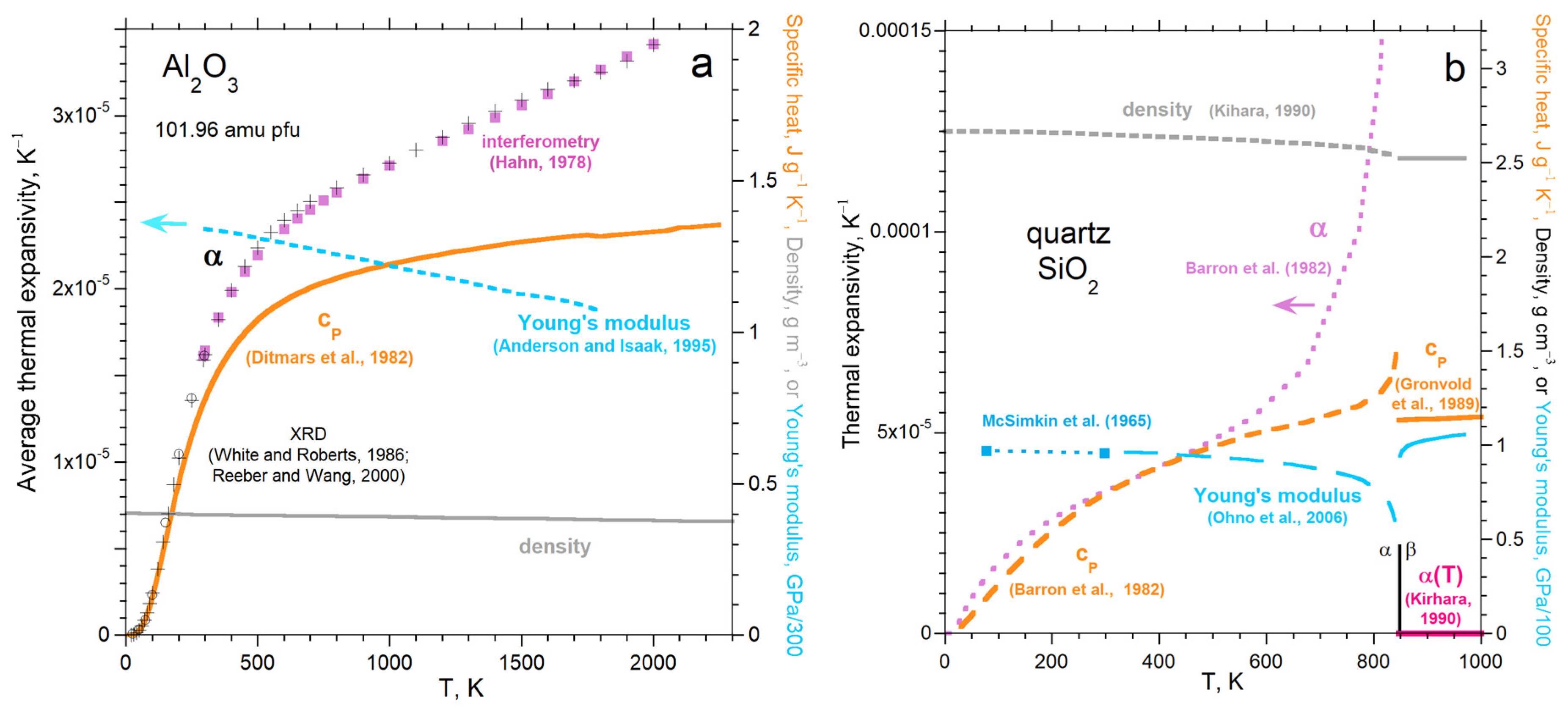
Below are two mineralogical examples on the correlation of highly accurate data on cP with αvol. Hofmeister [29] provides elemental Fe data up to melting temperatures. Hofmeister et al. [40] provide examples of Al, Mo, Ta, Au, diamond, Si, NaCl, KCl, MgO, and Y3Al5O12 garnet, and additional correlations of these physical properties.
Figure A1. Comparison of thermal expansivity to specific heat: (a) Al2O3. Plus = α from powder XRD compiled by [91]. Circle = α compiled by [92]. Pink squares = single-crystal interferometry and twin telemicroscope measurements [93]. Orange curve = cP compiled by [94]; aqua = elasticity data [95]. Grey = density calculated from α. Part a modified after Figure A1a in Hofmeister et al. [40], which has a Creative Commons license. (b) Properties low- and high-quartz polymorphs. Aqua dots = elasticity data from [96]; lavender = α and orange dashes = cP, both from [97]; orange bar from [98]; pink = α from [99]; aqua dashes = elasticity from [100]. Part b modified after Figure 15a in Hofmeister [29], which has a Creative Commons license.
Minerals 16 00509 g0a1

References

  1. Evans, B.W. The Serpentinite Multisystem Revisited: Chrysotile Is Metastable. Int. Geol. Rev. 2004, 46, 479–506. [Google Scholar] [CrossRef]
  2. Deer, W.A.; Howie, R.A.; Zussman, J. Rock-Forming Minerals, Volume 3B, Layered Silicates Excluding Micas and Clay Minerals, 2nd ed.; The Geological Society: London, UK, 2009; pp. 157–229. [Google Scholar]
  3. Nickel, E.H.; Hallberg, J.A.; Halligan, R. Unusual nickel mineralization at Nullagine, Western Australia. J. Geol. Soc. Aust. 1979, 26, 61–71. [Google Scholar] [CrossRef]
  4. Klein, F.; Bach, W.; Humphris, S.E.; Kahl, W.A.; Jöns, N.; Moskowitz, B.; Berquó, T.S. Magnetite in seafloor serpentinite—Some like it hot. Geology 2014, 42, 135–138. [Google Scholar] [CrossRef]
  5. Hofmeister, A.M. Measurements, Mechanisms, and Models of Heat Transport; Elsevier: Amsterdam, The Netherlands, 2019. [Google Scholar]
  6. Hofmeister, A.M.; Criss, R.E. A parameter-free model for temperature and pressure profiles in luminous, stable stars. High Temp.-High Press. 2023, 52, 435–464. [Google Scholar] [CrossRef]
  7. Horai, K. Thermal conductivity of rock-forming minerals. J. Geophys. Res. 1971, 76, 1278–1308. [Google Scholar] [CrossRef]
  8. Osako, M.; Yoneda, A.; Ito, E. Thermal diffusivity, thermal conductivity and heat capacity of serpentine (antigorite) under high pressure. Phys. Earth Planet. Inter. 2010, 183, 229–233. [Google Scholar] [CrossRef]
  9. Chien, Y.H.; Marzotto, E.; Tsao, Y.C.; Hsieh, W.P. Anisotropic thermal conductivity of antigorite along slab subduction impacts seismicity of intermediate-depth earthquakes. Nat. Commun. 2024, 15, 5198. [Google Scholar] [CrossRef] [PubMed]
  10. Kumzerov, Y.A.; Parfen’eva, L.S.; Smirnov, I.A.; Misiorek, H.; Mucha, J.; Jezowski, A. Thermal conductivity of crystalline chrysotile asbestos. Phys. Solid State 2003, 45, 57–60. [Google Scholar] [CrossRef]
  11. Wei, L.; Wang, D.; Zhang, R.; Yi, L. Thermal conductivity and thermal diffusivity of ophicarbonate at high temperature and pressure: Implications for the thermal structure of the oceanic lithosphere. J. Geophys. Res. Solid Earth 2025, 130, e2025JB032087. [Google Scholar] [CrossRef]
  12. Seipold, U.; Schilling, F.R. Heat transport in serpentinites. Tectonophysics 2003, 370, 147–162. [Google Scholar] [CrossRef]
  13. El Alami, K.; Bennouna El, G. Experimental Study of Serpentinite Rocks as Storage Materials for a Packed-bed Thermal Energy Storage System. Procedia Comput. Sci. 2025, 265, 770–775. [Google Scholar] [CrossRef]
  14. Hofmeister, A.M.; Pertermann, M.; Branlund, J.M. Thermal conductivity of the Earth. In Treatise in Geophysics; Schubert, G., Ed.; Elsevier: Amsterdam, The Netherlands, 2007; Volume 2, pp. 543–578. [Google Scholar]
  15. Hofmeister, A.M.; Branlund, J.M. Thermal conductivity of the Earth. In Treatise in Geophysics, 2nd ed.; Schubert, G., Ed.; Elsevier: Amsterdam, The Netherlands, 2015; Volume 2, pp. 584–608. [Google Scholar]
  16. Branlund, J.M.; Hofmeister, A.M. Thermal diffusivity of quartz to 1000 degrees C: Effects of impurities and the α-β phase transition. Phys. Chem. Miner. 2007, 34, 581–595. [Google Scholar] [CrossRef]
  17. Pertermann, M.; Hofmeister, A.M. Thermal diffusivity of olivine-group minerals. Am. Mineral. 2006, 91, 1747–1760. [Google Scholar] [CrossRef]
  18. Zhao, D.; Qian, X.; Gu, X.; Jajja, S.A.; Yang, R. Measurement techniques for thermal conductivity and interfacial thermal conductance of bulk and thin film materials. J. Electron. Packag. 2016, 138, 040802. [Google Scholar] [CrossRef]
  19. Gibert, B.; Schilling, F.R.; Gratz, K.; Tommasi, A. Thermal diffusivity of olivine single crystals and a dunite at high temperature: Evidence for heat transfer by radiation in the upper mantle. Phys. Earth Planet. Inter. 2005, 151, 129–141. [Google Scholar] [CrossRef]
  20. Kellett, B.S. Transmission of radiation through glass in tank furnaces. J. Soc. Glass Technol. 1952, 36, 115–123. [Google Scholar]
  21. Hofmeister, A.M. Thermodynamic and optical thickness corrections to diffusive radiative transfer formulations with application to planetary interiors. Geophys. Res. Lett. 2014, 41, 3074–3080. [Google Scholar] [CrossRef]
  22. Criss, R.E.; Hofmeister, A.M. The physical and mathematical meaning of temperature and its implications for astronomy. Galaxies 2025, 13, 118. [Google Scholar] [CrossRef]
  23. Vozár, L.; Hohenauer, W. Flash method of measuring the thermal diffusivity: A review. High Temp.-High Press. 2004, 36, 253–264. [Google Scholar] [CrossRef]
  24. Ikeda, K.; Yagi, K. Crystal-field spectra for blue and green diopsides synthesized in the join CaMgSi2O6-CaCrAlSiO6. Contrib. Mineral. Petrol. 1982, 81, 113–118. [Google Scholar] [CrossRef]
  25. Parker, W.J.; Jenkins, R.J.; Butler, C.P.; Abbot, G.L. Flash Method of Determining Thermal Diffusivity, Heat Capacity, and Thermal Conductivity. J. Appl. Phys. 1961, 32, 1679. [Google Scholar] [CrossRef]
  26. Corbin, S.F.; Turriff, D.M. Thermal Diffusivity by the Laser Flash Method. In Characterization of Materials; Kaufmann, E.N., Ed.; John Wiley and Sons, Inc.: New York, NY, USA, 2012; pp. 1–10. [Google Scholar]
  27. Hofmeister, A.M. Dependence of heat transport in solids on length-scale, pressure, and temperature: Implications for mechanisms and thermodynamics. Materials 2021, 14, 449. [Google Scholar] [CrossRef]
  28. Hofmeister, A.M. Experimental and theoretical evidence for heat being conducted in solids by diffusing infrared light. Therm. Conduct. 35/Therm. Expans. 2023, 23, 167–176. [Google Scholar]
  29. Hofmeister, A.M. Theory and Measurement of heat transport in solids: How rigidity and spectral properties govern behavior. Materials 2024, 17, 4469. [Google Scholar] [CrossRef]
  30. Degiovanni, A.; Andre, S.; Maillet, D. Phonic conductivity measurement of a semi-transparent material. In Thermal Conductivity 22; Tong, T.W., Ed.; Technomic: Lancaster, PA, USA, 1994; pp. 623–633. [Google Scholar]
  31. Hahn, O.; Hofmann, R.; Raether, F.; Mehling, H.; Fricke, J. Transient heat transfer in coated diathermic media: A theoretical study. High Temp.-High Press. 1997, 29, 693–701. [Google Scholar] [CrossRef]
  32. Hoffmann, R.; Hahn, O.; Raether, F.; Mehling, H.; Fricke, J. Determination of thermal diffusivity in diathermic materials by laser-flash technique. High Temp.-High Press. 1997, 29, 703–710. [Google Scholar] [CrossRef]
  33. Mehling, H.; Hautzinger, G.; Nilsson, O.; Fricke, J.; Hofmann, R.; Hahn, O. Thermal diffusivity of semitransparent materials determined by the laser-flash method applying a new mathematical model. Int. J. Thermophys. 1998, 19, 941–949. [Google Scholar] [CrossRef]
  34. Blumm, J.; Henderson, J.B.; Nilson, O.; Fricke, J. Laser flash measurement of the phononic thermal diffusivity of glasses in the presence of ballistic radiative transfer. High Temp.-High Press. 1997, 34, 555–560. [Google Scholar] [CrossRef]
  35. Hofmeister, A.M. Carryover of Sampling Errors and Other Problems in Far-Infrared to Far-Ultraviolet Spectra to Associated Applications. Rev. Mineral. Geochem. 2014, 71, 481–508. [Google Scholar] [CrossRef]
  36. Hsieh, W.P.; Chang, Y.Y.; Tsao, Y.C.; Lin, C.H.; Vilella, K. Exceptionally low thermal conduction of basaltic glasses and implications for the thermo-chemical evolution of the Earth’s primitive magma ocean. J. Geophys. Res. Solid Earth 2024, 129, e2023JB027722. [Google Scholar] [CrossRef]
  37. Hofmeister, A.M.; Sharp, M.G.; Whittington, A.G. Dependence of viscosity, thermal diffusivity, and thermal conductivity of East Pacific Rise pillow basalts, glasses, and melts on temperature and hydration. J. Volcanol. Geotherm. Res. 2026, 473, 108563. [Google Scholar] [CrossRef]
  38. Hofmeister, A.M. Lower mantle geotherms, flux, and power from incorporating new experimental and theoretical constraints on heat transport properties in an inverse model. Eur. J. Mineral. 2022, 34, 149–165. [Google Scholar] [CrossRef]
  39. Anderson, O.L.; Isaak, D.; Oda, H. High-temperature elastic constant data on minerals relevant to geophysics. Rev. Geophys. 1992, 30, 57–90. [Google Scholar] [CrossRef]
  40. Hofmeister, A.M.; Criss, E.M.; Criss, R.E. Thermodynamic relationships for perfectly elastic solids undergoing steady-state heat flow. Materials 2022, 15, 2638. [Google Scholar] [CrossRef] [PubMed]
  41. Hofmeister, A.M.; Dong, J.J.; Branlund, J.M. Thermal diffusivity of electrical insulators at high temperatures: Evidence for diffusion of phonon-polaritons at infrared frequencies augmenting phonon heat conduction. J. Appl. Phys. 2014, 115, 163517. [Google Scholar] [CrossRef]
  42. Merriman, J.D.; Whittington, A.G.; Hofmeister, A.M. A mineralogical model for thermal transport properties of rocks: Verification for low-porosity, crystalline rocks at ambient conditions. J. Petrol. 2023, 64, 1–30. [Google Scholar] [CrossRef]
  43. Incopera, F.P.; DeWitt, D.P. Fundamentals of Heat and Mass Transfer, 5th ed.; John Wiley and Sons: New York, NY, USA, 2002. [Google Scholar]
  44. Criss, E.M.; Hofmeister, A.M. Isolating lattice from electronic contributions in thermal transport measurements of metals and alloys and a new model. Int. J. Mod. Phys. B 2017, 31, 1750205. [Google Scholar] [CrossRef]
  45. Weber, J.N.; Greer, R.T. Dehydration of serpentine: Heat of reaction and reaction kinetics at PH2O = 1 ATM. Am. Mineral. 1965, 50, 450–464. [Google Scholar]
  46. Zhitova, E.S.; Krivovichev, S.V.; Pekov, I.; Greenwell, H.C. Crystal chemistry of natural layered double hydroxides. 5. Single-crystal structure refinement of hydrotalcite, [Mg6Al2(OH)16](CO3)(H2O)4. Mineral. Mag. 2019, 83, 269–280. [Google Scholar] [CrossRef]
  47. RRUFF: Comprehensive Database of Mineral Data. Available online: https://www.rruff.net/ (accessed on 1 March 2026).
  48. Armstrong, J.T. CITZAF, A package of correction programs for the quantitative electron microbeam X-ray analysis of thick polished materials, thin films, and particles. Microbeam Anal. 1995, 4, 177–200. [Google Scholar]
  49. Carpenter, P.K.; Vicenzi, E.P. Mineral reference standards and quantitative electron-probe microanalysis. Microsc. Microanal. 2012, 18, 1734–1735. [Google Scholar] [CrossRef]
  50. Przybyłowicz, W.; Szymczyk, S.; Kajfosz, J. Fluorine analysis in serpentinite rocks by proton induced gamma-ray emission. In Nuclear Instruments and Methods in Physics Research Section B: Beam Interactions with Materials and Atoms; Elsevier: Amsterdam, The Netherlands, 1986; Volume 15, pp. 573–575. [Google Scholar]
  51. Rao, K.V.; Purushottam, D.; Vaidyanadham, D. Uptake of fluoride by serpentine. Geochim. Cosmochim. Acta 1975, 39, 1403–1411. [Google Scholar] [CrossRef]
  52. Rietveld, H.M. A Profile Refinement Method for Nuclear and Magnetic Structures. J. Appl. Crystallogr. 1969, 2, 65–71. [Google Scholar] [CrossRef]
  53. Young, R.A. Introduction to the Rietveld method. In The Rietveld Method; Young, R.A., Ed.; IUCr Book Series; Oxford University Press: Oxford, UK, 1993; pp. 1–39. [Google Scholar]
  54. Balzar, D. Voigt-function model in diffraction line broadening analysis. In Microstructure Analysis from Diffraction; Snyder, R.L., Bunge, H.J., Fiala, J., Eds.; International Union of Crystallography: Chester, UK, 1999. [Google Scholar]
  55. Blumm, J.; Opfermann, J. Improvement of the mathematical modeling of flash measurements. High Temp.-High Press. 2002, 34, 515–521. [Google Scholar] [CrossRef]
  56. Min, S.; Blumm, J.; Lindemann, A. A new laser flash system for measurement of the thermophysical properties. Thermochim. Acta 2007, 455, 46–49. [Google Scholar] [CrossRef]
  57. McMasters, R.L.; Beck, J.V.; Dinwiddie, R.B.; Wang, H. Accounting for penetration of laser heating in flash thermal diffusivity experiments. J. Heat Transf. 1999, 121, 15–21. [Google Scholar] [CrossRef]
  58. Huggins, C.W.; Shell, H.R. Density of bulk chrysotile and massive serpentine. Am. Mineral. 1965, 50, 1058–1067. [Google Scholar]
  59. Cervelle, B.D.; Maquet, M. Cristallochimie des lizardites substituees Mg-Fe-Ni par spectrometrie visible et infrarouge proche. Clay Miner. 1982, 17, 377–392. [Google Scholar] [CrossRef]
  60. Rossman, G.R. Optical spectroscopy. Rev. Mineral. 1988, 18, 207–254. [Google Scholar]
  61. Hofmeister, A.M.; Rossman, G.R. Determination of Fe3+ and Fe2+ concentrations in feldspar by optical and EPR spectroscopy. Phys. Chem. Miner. 1984, 11, 213–224. [Google Scholar] [CrossRef]
  62. Fenstermacher, J.E. Optical absorption due to tetrahedral and octahedral ferric iron in silicate glasses. J. Non-Cryst. Solids 1980, 38, 239–244. [Google Scholar] [CrossRef]
  63. Lehmann, G.; Harder, H. Optical spectra of di-and trivalent iron in corundum. Am. Mineral. 1970, 55, 98–105. [Google Scholar]
  64. Kats, A. Hydrogen in a-quartz. Philips. Res. Repts. 1962, 17, 113–195, 201–279. [Google Scholar]
  65. Rockett, T.J.; Foster, W.R. The thermal stability of purified tridymite. Am. Mineral. 1967, 52, 1233–1240. [Google Scholar]
  66. Hofmeister, A.M.; Bowey, J.E. Quantitative IR spectra of hydrosilicates and related minerals. Mon. Not. R. Astron. Soc. 2006, 367, 577–591. [Google Scholar] [CrossRef]
  67. Hofmeister, A.M. Thermal diffusivity and thermal conductivity of single-crystal MgO and Al2O3 as a function of temperature. Phys. Chem. Miner. 2014, 41, 361–371. [Google Scholar] [CrossRef]
  68. Merriman, J.M.; Hofmeister, A.M.; Whittington, A.G.; Roy, D.J. Temperature-dependent thermal transport properties of carbonate minerals and rocks. Geophere 2018, 14, 1961–1987. [Google Scholar] [CrossRef]
  69. Candela, P.A.; Crummett, C.D.; Earnest, D.J.; Frank, M.R.; Wylie, A.G. Low-pressure decomposition of chrysotile as a function of time and temperature. Am. Mineral. 2007, 92, 1704–1713. [Google Scholar] [CrossRef]
  70. Trittschack, R.; Grobéty, B.; Koch-Müller, M. In situ high-temperature Raman and FTIR spectroscopy of the phase transformation of lizardite. Am. Mineral. 2012, 97, 1965–1976. [Google Scholar] [CrossRef]
  71. Sawai, M.; Katayama, I.; Hamada, A.; Maeda, M.; Nakashima, S. Dehydration kinetics of antigorite using in situ high-temperature infrared microspectroscopy. Phys. Chem. Miner. 2013, 40, 319–330. [Google Scholar] [CrossRef]
  72. King, E.G.; Barany, R.; Weller, W.W.; Pankratz, L.B. Thermodynamic Properties of Forsterite and Serpentine; US Department of the Interior, Bureau of Mines: Washington, DC, USA, 1967; Volume 6962. [Google Scholar]
  73. Guggenheim, S.; Zhan, W. Effect of temperature on the structures. Can. Mineral. 1998, 36, 1587–1594. [Google Scholar]
  74. Harwood, C.; Yates, B.; Badami, D.V. The thermal expansion of chrysotile asbestos and its composites. J. Mater. Sci. 1979, 14, 1126–1140. [Google Scholar] [CrossRef]
  75. Nestola, F.; Angel, R.; Zhao, J.; Garrido, C.; Sánchez-Vizcaíno, V.; Capitani, G.; Mellini, M. Antigorite equation of state and anomalous softening at 6 GPa: An in situ single-crystal X-ray diffraction study. Contrib. Mineral. Petrol. 2010, 160, 33–43. [Google Scholar] [CrossRef]
  76. Yang, C.; Inoue, T.; Yamada, A.; Kikegawa, T.; Ando, J.I. Equation of state and phase transition of antigorite under high pressure and high temperature. Phys. Earth Planet. Inter. 2014, 228, 56–62. [Google Scholar] [CrossRef]
  77. Hilairet, N.; Daniel, I.; Reynard, B. P–V equations of state and the relative stabilities of serpentine varieties. Phys. Chem. Miner. 2006, 33, 629–637. [Google Scholar] [CrossRef]
  78. Bose, K.; Navrotsky, A. Thermochemistry and phase equilibria of hydrous phases in the system MgO-SiO2-H2O: Implications for volatile transport to the mantle. J. Geophys. Res. Solid Earth 1998, 103, 9713–9719. [Google Scholar] [CrossRef]
  79. Fei, Y. Thermal Expansion. In Mineral Physics and Crystallography; Ahrens, T.J., Ed.; A Handbook of Physical Constants; American Geophysical Union: Washington, DC, USA, 1995; pp. 29–44. [Google Scholar]
  80. Bezacier, L.; Reynard, B.; Cardon, H.; Montagnac, G.; Bass, J.D. High-pressure elasticity of serpentine and seismic properties of the hydrated mantle wedge. J. Geophys. Res. Solid Earth 2013, 118, 527–535. [Google Scholar] [CrossRef]
  81. Wang, D.; Liu, T.; Chen, T.; Qi, X.; Li, B. Anomalous sound velocities of antigorite at high pressure and implications for detecting serpentinization at mantle wedges. Geophys. Res. Lett. 2019, 46, 5153–5160. [Google Scholar] [CrossRef]
  82. Mayhew, L.E.; Ellison, E.T. A synthesis and meta-analysis of the Fe chemistry of serpentinites and serpentine minerals. Phil. Trans. R. Soc. Lond. A Math. Phys. Eng. Sci. 2020, 378, 2165. [Google Scholar] [CrossRef]
  83. Evans, B.W.; Dyar, M.D.; Kuehner, S.M. Implications of ferrous and ferric iron in antigorite. Am. Mineral. 2012, 97, 184–196. [Google Scholar] [CrossRef]
  84. Krzeminski, S.F.; Straub, D.K. Mossbauer spectra of trispyrrolidylcarbodithioates of Cr(III), Co(III), Ga(III), and In(III) doped with Fe(III). Evidence of cross relaxation between Fe(III)–Cr(III). J. Chem. Phys. 1973, 58, 1086–1089. [Google Scholar] [CrossRef]
  85. Jezowski, A.; Mucha, J.; Pompe, G. Thermal conductivity of the amorphous alloy Fe40Ni40P14B6 between 80 and 300 K. J. Phys. D Appl. Phys. 1987, 20, 1500–1506. [Google Scholar] [CrossRef]
  86. Seipold, U. Simultaneous measurements of thermal diffusivity and conductivity under high pressure by thermal pulses of finite length. High Temp.-High Press. 1988, 20, 609–613. [Google Scholar]
  87. Cowan, D.R. Pulse method of measuring thermal diffusivity at high temperatures. J. Appl. Phys. 1963, 34, 926–927. [Google Scholar] [CrossRef]
  88. Osako, M.; Ito, E.; Yoneda, A. Simultaneous measurements of thermal conductivity and thermal diffusivity for garnet and olivine under high pressure. Phys. Earth Planet. Inter. 2004, 143–144, 311–320. [Google Scholar] [CrossRef]
  89. Hofmeister, A.M. Thermal diffusivity of orthopyroxenes at elevated temperature. Eur. J. Mineral. 2012, 24, 669–681. [Google Scholar] [CrossRef]
  90. Hofmeister, A.M.; Criss, R.E. Spin, orbit, drag, and phase equilibria control of Uranus’ surface and atmospheric conditions: Planetary implications. Planet. Space Sci. 2026, 275, 106268. [Google Scholar] [CrossRef]
  91. Reeber, R.R.; Wang, K. Lattice parameters and thermal expansion of important semiconductors and their substrates. MRS Proc. 2000, 622, 1–6. [Google Scholar] [CrossRef]
  92. White, G.K.; Roberts, R.B. Thermal expansion of reference materials: Tungsten and α-Al2O3. High Temp.-High Press. 1983, 15, 321–328. [Google Scholar]
  93. Hahn, T.A. Thermal expansion of single crystal sapphire from 293 to 2000 K, Standard reference material 732. In Thermal Expansion 6; Springer: Boston, MA, USA, 1978; Volume 6, p. 191. [Google Scholar]
  94. Ditmars, D.A.; Ishihara, S.; Chang, S.S.; Bernstein, G.; West, E.D. Enthalpy and heat capacity standard reference material: Synthetic sapphire (α-Al2O3) from 10 to 2250 K. J. Res. Natl. Bur. Stand. 1982, 87, 159–163. [Google Scholar] [CrossRef] [PubMed]
  95. Anderson, O.L.; Isaak, D. Elastic constants of mantle minerals at high temperatures. In Mineral Physics and Crystallography. A Handbook of Physical Constants; Ahrens, T.J., Ed.; American Geophysical Union: Washington, DC, USA, 1995; Volume 2, pp. 64–97. [Google Scholar]
  96. McSkimin, H.J.; Andreatch, J.P.; Thurston, R.N. Elastic moduli of quartz versus hydrostatic pressure at 25 °C and −195.8 °C. J. Appl. Phys. 1965, 36, 1624–1632. [Google Scholar] [CrossRef]
  97. Barron, T.H.K.; Collins, J.F.; Smith, T.W.; White, G.K. Thermal expansion, Gruneisen functions and static lattice properties of quartz. J. Phys. C Solid State Phys. 1982, 15, 4311. [Google Scholar] [CrossRef]
  98. Grønvold, F.; Stølen, S.; Svendsen, S.R. Heat capacity of α quartz from 298.15 to 847.3 K, and of β quartz from 847.3 to 1000 K—Transition behaviour and revaluation of the thermodynamic. Thermochim. Acta 1989, 139, 225–243. [Google Scholar] [CrossRef]
  99. Kihara, K. An X-ray study of the temperature dependence of the quartz structure. Eur. J. Mineral. 1990, 2, 63–77. [Google Scholar] [CrossRef]
  100. Ohno, I.; Harada, K.; Yoshitomi, C. Temperature variation of elastic constants of quartz across the α-β transition. Phys. Chem. Miner. 2006, 33, 1–9. [Google Scholar] [CrossRef]
Figure 3. Visible spectra, with assignments and sample numbers in different colors for each sample, as labelled (1100 nm corresponds to 9091 cm−1 and 250 nm corresponds to 40,000 cm−1). Thicknesses listed are of each disk, which were used in Equation (14) to provide A shown here. Vertical lines in different colors show peak assignments (Appendix A). Notably, Fe3+ tet and Cr3+ oct both absorb at 450 to 460 nm. (a) Lizardites. The liz-T spectrum from the thicker disk (blue dashes) was shifted downwards to match the thinner data collection, which had less physical scattering, likely from grain boundaries. Data below 325 nm exist, but are not included due to physical scattering and low throughput creating artifacts. (b) Antigorite, chrysotiles, and Ni-rich samples. Ni-Fe lizardite is a secondary phase accompanying pecoraite, which occurs as plates, so the latter spectra record both a and c directions. Chrysotiles were oriented ⊥ to the tubules.
Minerals 16 00509 g003
Figure 4. Total Al (dots) and total Fe cations (squares) in our serpentine formula (Table 1: ideally Mg3Si2O5(OH)4), compared to the number of H atoms over 4, obtained from EPMA. Total oxides are below 99.1%. The bulk sample of lizardite G has chlorite, which may affect partitioning and availability of water.
Minerals 16 00509 g004
Figure 6. Unpolarized near-infrared spectra, uncorrected for surface reflections and scattering, from antigorite disks prior to use in LFA measurements and thinner slices. Thicknesses refer to the samples: this value was used in Equation (15) to compute A. (a) Antigorite 100 face. Spectra were scaled to best match shared features. The noisy region exists for the thick section (aqua) where throughput is negligible, so the calculated A is distorted. Comparing weak features suggests that the small chip thickness was ~0.12 mm rather than 0.04 mm recorded. (b) Antigorite 010 face. Scaling confirms thickness of the chip. Purple represents the thick section.
Minerals 16 00509 g006
Figure 7. Near-IR spectra. (a) Lizardites. Liz-M2 after LFA (green curve) to 910 K was scaled to match the lattice overtones of a random chip of the lizardite-T (black curve). Forsterite peaks in the heated sample are masked by either noise below 1800 cm−1 or by the OH peak. (b) Chrysotile (⊥a) compared to antigorite (aqua). Fibers are about 0.1 mm across forming a mat. Thickness was not measured but involves stacked fibers to block stray light. Thick vertical bars mark the O-H fundamentals and their first overtones. Peak positions of the M-O-H bending modes are similar to those in antigorite (blue curve) and in lizardite (right panel), indicating that the O-H sites are similar.
Minerals 16 00509 g007
Figure 9. Interdependence of the fitting parameters for solids with mostly ionic bonding. Grey dot and curve = 134 minerals and related substances compiled in [5,41]. Black diamond = rock data [5,42]. Purple crosses from [68]. Data on chrysotile ||a (blue square) was limited to 500 K, so three possibilities from Table 4 are shown. Red squares = remaining serpentines. Due to the flat trends, it was difficult to ascertain parameter H for antigorite 001, pecoraite, and chrysotiles ⊥a.
Minerals 16 00509 g009
Figure 11. Literature data on cP and volumetric α as a function of temperature from the sources in Table 5. Green triangles from [13] Blue diamonds and circles from [72]. Maier–Kelly fits in Table 5 poorly extrapolate to low T. Fits are singular as T ⟶ 0 K. Least squares fits provide αvol = 5.618 + 0.12984T − 6.1443 × 10⁻⁵ T2 with R2 = 0.995 for averaging the 3 directions of hot-pressed chrysotile (red open squares from [73]). At high-T, antigorite enthalpy was measured [72], which provides a linear dependence for cP vs. T. Adiabatic calorimetric below 298 K is much more accurate, ±0.5% [72]. Open pink diamonds = αvol from XRD for antigorite [76,78]; green down-pointing triangle = αvol from XRD from [73]. Orange hexagon = αvol = calculated in Section 5.2.
Minerals 16 00509 g011
Table 1. Sample characteristics.
Sample *Description LocalitySource Formulae §
Antigorite apale gray green blockCedar Hill Quarry, Lancaster Co., Peach Bottom, PA, USAExcaliburMg2.900Fe2+0.034Al0.076[Al0.075Si1.987]O9H4.13
(ΣM = 3.011; ΣT = 2.062) Fe3+/Fetot~0
Lizardite-Mpale green block Montville, NJ, USAWU481-18Ca0.003Mg2.958Mn3+0.003Al0.017Fe3+0.011[Fe3+0.034Ti0.002Si1.964]
O9H4.067Cl0.003 (ΣM = 3.022; ΣT = 2) Fe3+/Fetot~1
Serpentine-Ggreen block
± chlorite
GermanyWU481-28Na0.012Ca0.003Mg2.968Al0.020[Fe3+0.050Al0.024Si1.926]
O9H4.150Cl0.034 (ΣM = 3.003; ΣT = 2) Fe3+/Fetot~1
Serpentine-S1dark green block
± calcite veins
Snarum, NorwayWU481-24Ca0.004Mg2.932Fe2+0.015Fe3+0.015Al0.036[Fe3+0.029Al0.035Ti0.001Si1.925]
O9H4.150Cl0.001 (ΣM = 3; ΣT = 1.99) Fe3+/Fetot~0.75
Serpentine-Wcream color,
fibrous + calcite
Snarum, NorwayWU481-24Mg2.963Fe2+0.010Fe3+0.004Al0.026[Fe3+0.03Ti0.001Si1.969]O9H3.984
(ΣM = 3.003; ΣT = 2) Fe3+/Fetot~0.77
Lizardite-T bsmall green block, 2 phasesArgent Tunnel,
Tasmania
SM-R10581Ca0.002Mg2.896Fe2+0.017Fe3+0.029Al0.054[Fe3+0.067Cr0.016Si1.917]
O9H4.096Cl0.040 (ΣM = 2.998; ΣT = 2) Fe3+/Fetot~0.85
Al-lizardite cyellow-green block ± bruciteSnarum, Vikersund, NorwayExcaliburMg2.853Fe3+0.059Al0.152[Fe3+0.060Al0.377Si1.563]O9H4.226Cl0.013
(ΣM = 3.064; ΣT = 2.0) Fe3+/Fetot~1
Chrysotile-B apale gray tubules
+ magnetite blebs
Bell Mine, Thetford,
Quebec, QC, Canada
WU481-45poor polish: Mg~Si > Al~Fe;
Na, Mn, K, P, Ni, Cr, Ca, S, Co bld
Chrysotile-T apale green tubules
± magnetite ends
Thetford, Quebec,
Canada
WU481-67n.m. Fe3+/Fetot~0 e
Chrysotile-G1 apale yellow tubules
+ rare magnetite
Globe, AZ, USAWU481-52Na0.006Ca0.002Mg2.983Mn3+0.002Fe3+0.007[Al0.004Si1.998]O9H3.984
(ΣM = 3.00; ΣT = 2.002) Fe3+/Fetot~1
Chrysotile-G2 apale yellow tubules
+ magnetite
Globe, AZ, USAWU481-55n.m.
Pecoraite dbright green curved
plates + metal oxide
Otway Prospect,
Nullagine,
W. Australia
ExcaliburCa0.003Mg0.194Mn0.003Co0.005Ni2.668Cr0.130
[Cr0.259Fe3+0.034Si1.697P0.010]O9H4.123
(ΣM = 3.004; ΣT = 2) Fe3+/Fetot~1
Ni-Fe-lizardite dtiny yellow blocks dpart of pecoraite Ca0.008Mg2.689Ni0.073Fe3+0.131Cr0.017Al0.085
[Al0.086Fe3+0.070Si1.833Ti0.011]O9H4.003
(ΣM = 3.003; ΣT = 2) Fe3+/Fetot~1
* Polymorph determined by XRD analysis. Magnetite is present in many samples. Phases found in EPMA or observed using a binocular microscope. WU = Washington University collection. SM = Smithsonian Museum. Excalibur = purchase. § Formulae from EPMA, where charge state and site occupancy were ascertained from visible spectroscopy and then Al and Cr were assigned in accord with stoichiometry and charge conservation, see below. Site occupancies 0.001 and below are omitted. a Samples which could be oriented by foliation or cleavage. b Mostly lizardite according to Weber and Greer [45]. Two phases with nearly identical compositions were observed in microprobe analysis. c Associated with hydrotalcite [46], which was not detected in our sample. The RRUFF [47] database specified lizardite-1T. Disk c of this Al-rich material contained brucite per XRD (Section 3.4). d See Nickel et al. [3]. Our rock sample similarly has gaspeite (Ni-Mg-Fe carbonate), trevorite (NiFe3+2O4), and maghemite (γ-Fe2O3) per XRD. The formula for the secondary serpentine phase in this rock (yellow Ni-Fe-lizardite) is an average of assuming ferric and ferrous iron in EPMA. No Fe2+ was detected, but is suggested by charge balance. e Visible spectra of pale green Thetford chrysotile show Fe2+, but little if any Fe3+.
Table 2. Chemical composition from EPMA (in oxide wt%) of individual serpentine phases *.
wt%antig.liz-Mserp-Gserp-S1 bserp-S2 cserp-Wliz-T
Main
liz-T
inter. d
Al-lizchry-G1PecoraiteNi-Fe-liz
SiO241.6841.8840.2440.7441.8541.5540.5941.73732.0342.5026.2137.40
TiO20.0020.0570.0230.0260.0110.0260.0100.0050.0090.003bld0.308
Al2O30.2730.3140.7051.270.5950.4590.9730.4169.390.0680.0112.96
Cr2O30.0030.0100.0150.005bldbld0.4270.5240.001bld7.570.434
Fe2O3 a---1.6551.7031.224---0.1950.7025.51
FeO a0.8471.1401.244---2.8531.6812.90---
MgO40.7942.3141.6142.3141.5241.9341.1241.1239.2042.562.0036.85
MnO0.0070.0850.0190.0190.0440.0310.01400.0130.0010.0400.0530.035
NiO----bldbld---bld50.951.85
CoO----0.005bld---bld0.0970.005
ZnO------0.01370.014----
CaO0.0070.0520.0530.0230.08230.0040.0400.0260.0130.0340.0450.147
Na2Obld0.0150.1320.0170.0050.00170.0060.0100.0040.065bldbld
K2Obld0.0050.014bldbldbld0.0100.0030.050bld0.0030.006
P2O5----bldbld0.0060.004-0.0080.1900.030
SO3----0.1010.011--.-0.0700.0410.005
Clbld0.0420.4180.026--0.0400.026bld---
H2O a1313131312.712.613131312.79.512.5
Total a96.6198.8997.3898.3798.5997.7999.0998.8696.6798.1897.3798.03
Fe/(Fe + Mg)0.01150.01500.01660.0197 0.01460.03760.02220.04000.0023§§
* Averages of three datapoints are given. The last digit is uncertain. Uncertainties are roughly ±2%. The dash indicates that this element was not probed. bld = below the detection limit. a The software computes either FeO or Fe2O3 from the measured Fe wt%. The conversion factor is 1.113 × FeO wt% to provide Fe2O3. Values of H2O were chosen in order to provide a reasonable stoichiometry. Both choices determine the totals, which remain low, despite well-polished surfaces (excepting fibrous chrysotile). b Dark green Snarum serpentine used in LFA. c Light green Snarum serpentine (S2) grades into the white fibrous regions, but was not studied by LFA. The formula for S2 is Ca0.004Mg2.912Mn0.002Fe2+0.027Al0.033[Fe3+0.033Si1.969]O9H3.986 (ΣM = 3.006; ΣT = 2.002). d The interstitial phase in liz-T is volumetrically tiny compared to the main phase. Its formula is Mg2.903Fe2+0.066Cr0.020[Al0.023Si1.963]O9H4.078Cl0.026 (with ΣM = 2.989; ΣT = 1.986 and Fe3+/Fetot~0. Trace amounts of ZnO and P2O5 were detected in both phases of lizardite-T. § Pecoraite is 88.8% Ni endmember; Ni-Fe lizardite is 2.4% Ni endmember and 89.5% Mg endmember.
Table 3. XRD determination of mineralogy (in wt%) of the serpentine phases.
SampleFormInitial Phases *Post FormTmax, KProduct Phases *
Antigorite(001) diskantigorite(010) powder90592% atg (21 μm) + 8% for (30 μm)
(100) diskantigorite(100) disk855antigorite
Lizardite-Mpowder §97% liz (32 μm) + 3% mag (45 μm)M1 disk1080forsterite
M2 disk91068% liz 1T (1 mm) + 32% for (32 μm)
Serpentine-Gpowder §55% liz (32 μm) + 45% clinochlore (32 μm)disk85573% liz 1T (14 μm) + 27% for (47 μm)
Serpentine-Spowder §96% liz (20 μm) + 4% mag (25 μm)disk S1a78580% liz (31 μm) + 20% for (50 μm)
Serpentine-Wdisk85% liz (4 μm) + 8% chry 2Mc1 (30 μm) + 7% calcite (80 μm)disk77078% liz (6 μm) + 13% chry 2Mc1 (23 μm) + 9% calcite (110 μm)
Lizardite-T-~liz (Weber and Greer [46])disk785lizardite 1T
Al-lizardite #powder §91% liz (32 μm) + 9% brucite (54 μm) + sapponite disk a90055% liz (20 μm) + 45% for (62 μm)
Al-serpentine #disk b765lizardite 1T
Al-serpentine #disk c76597% liz (31 μm) + 3% brucite (65 μm)
Chrysotile-Bfiber matchrysotile 2Mc1 @fiber mat765n.m.
Chrysotile-G1fiber matchrysotile 2Mc1 @fiber mat765n.m.
Pecoraite powder §pecoraite 2Mc1 + major trevorite +
minor gaspeite + minor maghemite
disk76580% nepouite 1T (9 μm)
+ 20% mag (45 μm)
* Indicates proportions in wt% and crystal sizes from Rietveld, which are approximate due to preferred orientation. Atg denotes antigorite; liz = lizardite 1T; chry = chrysotile; for = forsterite; mag = magnetite. Sappingtonite (indicated by the Eva software) is not in the Rietveld database. Proportions are low from Eva. Hydrotalcite is noted in the literature but was not detected by XRD. Pecoraite is not in the Rietveld database. Rough proportions are suggested by the Eva program. End-member trevorite is NiFeO4; maghemite is γ-Fe2O3 with the spinel structure, and so this starting material has largely ferric iron. § Powders of the starting material represent a larger portion of the sample: several measurements include more phases than the disks measured in LFA. These impurities are likely present in the disks, but in smaller amounts than in the powder. # Brucite was detected in disk c of Al-rich serpentine, which is consistent with disk c dehydrating below 700 K in LFA runs, and is thus denoted serpentine. Disk a did not dehydrate until 800 K was reached, consistent with lizardite. Disk b apparently has impurities, in view of low-T dehydration during LFA runs (Section 4.5). @ Only chrysotile peaks were observed, so a Rietveld refinement was not performed. Magnetite is below the limit of detection.
Table 4. Thermal diffusivity initial values and fitting parameters *.
Sample LTinitDR.T.D = FT−G + HT (mm2 s−1)R2DR.T.,post &
mm°Cmm2 s−1FGH × 105 mm2 s−1
Antigorite 1001.1021.10.74915.208 ± 4.70.54505 ± 0.5720.243 ± 3.90.9950.755
Antigorite 0101.4021.21.43630.55 ± 4.40.54759 ± 0.0002625.545 ± 3.60.9991.496
Antigorite 0010.9920.90.4903.1324 ± 0.30.32586 ± 0.016≡00.9860.493
Antigorite average~1 21.00.81421.219 ± 8.80.58631 ± 0.0821.249 ± 5.50.992-
Lizardite-M11.3921.01.1134.688 ± 150.61082 ± 0.0816.276 ± 80.994
M1 (forsterite) 1.3990.089 ± 130.80146 ± 0.0317.29 ± 1.30.9991.00
Lizardite-M20.7920.91.31124.08 ± 800.81957 ± 0.1131.35 ± 110.9891.23
Lizardite-M3 a1.5520.31.46 &113.33 ± 110.77926 ± 0.0231.585 ± 20.9991.50
Lizardite-M3 b1.18520.51.408 &79.61 ± 80.72063 ± 0.0225.049 ± 20.9991.40
Lizardite-M3 c1.16520.51.365 &102.28 ± 120.77249 ± 0.0231.439 ± 20.999-
Serpentine-G1.4021.50.976 186.39 ± 610.94562 ± 0.0638.398 ± 30.9981.08
Serpentine-S1 a1.1221.01.04201.66 ± 730.95082 ± 0.06543.906 ± 40.9961.035
Serpentine-S1 b3.0120.51.259 &-----
Serpentine-W 0.78 20.60.910 &57.365 ± 140.72495 ± 0.0410.858 ± 30.9980.779
Lizardite-T0.7022.70.981113.69 ± 390.85574 ± 0.0638.7 ± 40.9980.955
Al-lizardite a1.2420.81.507305.66 ± 1700.94444 ± 0.120.68 ± 9.60.9980.811
Al-Serpentine b0.7920.41.475 &159.94 ± 220.83506 ± 0.02526.167 ± 30.9991.167
Al-serpentine c1.4320.11.405 &93.854 ± 130.74302 ± 0.0257.9532 ± 30.9991.031
Chrysotile-T⊥a1.2020.50.564 &-----
Chry-T||a + mag7.3020.54.31 ± 0.1 #&471.04 ± 1290.82728 ± 0.05≡00.983-
fit with linear term---1693.5 ± 25761.0621 ± 0.2890.246 ± 930.985-
preferred Chry-T ||a---916.55 ± 22≡0.9551.253 ± 180.985-
Chry-B ⊥a + much mag2.5620.50.761 &51.22 ± 21.50.7509 ± 0.0817.425 ± 4.40.9930.67
Chrysotile-G ⊥a0.7520.50.325 &17.654 ± 4.880.7338 ± 0.0517.101 ± 1.10.9900.31
Chry-G ⊥a + mag2.8020.50.51 &-----
Chrysotile-G ||a8.0020.53.9 ± 0.8 #&-----
Chrysotile average #Varies20.51.06 &107.08 ± 150.82306 ± 0.02619.024 ± 2.00.999-
Pecoraite plates §1.3520.50.565 &30.524 ± 250.71664 ± 0.1516.816 ± 8.80.991
Nepouite + mag1.35<600~0.41 &D = 0.5676 − 0.00031377T (high T data only)0.9930.407
* Coefficient G has no units. Units of coefficient F depend on the value of G. Coefficient H has units of mm2 s−1 K−1. High uncertainties in coefficient F are due to tradeoffs in fitting exponent G. To reproduce the data, all digits that are shown for F, G, and H are needed. Numbers (e.g., M1 and M2) indicate different pieces of the same sample. Letters (a, b, c) indicate perpendicular cuts of one piece of a given sample. Sample transformed. The post-run value was used as the starting value for forsterite. This data is shown for comparative purposes only. Fit to serpentine W, which is largely perpendicular to the a-axis, is affected by a gradual transition from lizardite to chrysotile ⊥a (Table 3), providing lower D. # Averages are based on morphology, not degeneracy of crystallographic axes. Uncertainties are large for chrysotiles oriented parallel to the a-axis because the samples were macroscopic cylinders, not disks, causing additional 2-dimensional heat flow. Runs were terminated at low T, due to increasing uncertainty. Data on chrys-G ||a were uncertain, but confirm high D for chrys-T ||a. § Pecoraite occurred as curved platelets that were similarly oriented. The morphology is consistent with unrolled tubules and so approximates 1:1 mixture of the crystallographic axes. Oxide impurities are present, from the appearance. & More accurate measurements made with the LFA-467. Post-run data collected with the LFA-467 are listed with more significant figures.
Table 5. Properties used to calculate K for bulk serpentine minerals and mixtures.
ρ(298 K)
(kg m−3)
cP(298 K)
(J/g-K)
cP(T)
(J/g-K)
T Range
(K)
αvol
(K−1)
T Range
(K)
B + BP *
(GPa)
Antigorite2620 *&$0.910 −1.2191 − 0.0028797T
+ 508.3T−2 + 0.1722T½ †
50–300;
400–847
3.9 × 10⁻⁵ $
2.93(7) × 10−5 ^
298–775
473–873
62.9 + 6.1P &$
Lizardite2610 *@---1.87 × 10⁻⁵ #298–80068.9 @
Chrysotile2570 *@0.911 Close to antigorite 50–3004.0 × 10−5 §80–27062 ± 2 @
Serpentinite~2620 0.939 8.1701 + 0.0081558T
− 151720T−2 − 0.46075T½ ‡
300–850---
* Density from room temperature XRD data. Compression studies assumed B’ = ∂B/∂T = 4 except for antigorite, see text for discussion. Molar weight = 300.77 g for endmember serpentine was used to convert high-T enthalpy and cryogenic cP data of King et al. [72] to a per gram basis. Residual R2 of the fit, which combined low- and high-T datasets, is 0.998. Skeletal density for sample SPR2 of El Alami and Bennouna [13], who measured cP using digital scanning calorimetry. SPR2 is described as >85% serpentine (mostly lizardite) with magnesioferite, and having a bulk density ~2520 kg m−3 with porosity ~5%. Fit has R2 = 0.999. # The reported α was obtained from a linear fit of volume vs. temperature reported by Guggenheim and Zhan [73], and thus represents the midpoint T of 550 K. § Chrysotile from the Cassiar mine in Northern British Columbia, which has ~5 wt% FeO [2]. We report the sum of linear thermal expansivities for three perpendicular directions of a hot-pressed bar of aligned chrysotile measured using Fizeau interferometry by Harwood et al. [74]. A composite with resin was pressed to 3.86 × 10⁶ N−2 at~425 K for 30 min. Porosity was ~1%. & Nestola et al. [75]. $ Yang et al. [76]. @ Hilariet et al. [77]. Bulk density is lower, 2190 to 2390 kg m−3 for chrysotiles with magnetite [55], due to porosity. ^ Bose and Navrotsky [78].
Table 6. Thermal conductivity of serpentine minerals and mixtures.
SampleD-Values UsedK(298 K) *
Wm−1 K−1
K(T)
Wm−1 K−1
R2K/∂P|0(298)
Wm−1 K−1 GPa−1
Antigorite1001.790.9517 − 0.0014229T − 9426.1T−2 + 0.077021T½0.9990.202
0103.432.607 − 0.0025599T − 26105T−2 + 0.10559T½0.9990.387
0011.170.37899 − 0.0019004T − 11430T−2 + 0.085357T½0.9990.132
bulk1.921.3429 − 0.0012608T − 11052T−2 + 0.062628T½0.9990.217
Lizarditebulk
(liz-M1)
2.642.7542 − 0.0013321T − 22688T−2 + 0.030518T½0.9990.300
Chrysotile @a0.760.29684 − 0.00024909T − 1309.88T−2 + 0.029213T½0.9990.086
||a10.118.339 + 0.0055522T − 50517T−2 − 0.55655T½0.9991.14
bulk §2.483.5709 + 0.00041032T − 14355T−2 − 0.064943T½0.9990.280
SerpentineLiz + chrys
(liz-T)
2.322.3063 + 0.00023257T − 606.18T−2 − 0.0029875T½0.9800.262
Serpentiniteserp-G2.4727.663 + 0.03084T − 401390T−2 − 1.7544T½0.9840.39
* Uses measurements of cP, and mineral density which does not address porosity. Accuracy is within 3% except for serpentinite, for which the approximate D at 298 K and digital scanning calorimetry from [13] were used. Uses bulk density and the fit to cP data (Table 5), which differ slightly from the measurements at ambient T, due to the linear high-T trend (see Figure 12). Initial values used an average B0 = 64 ± 2 GPa, which holds to ~25 GPa. This calculation describes bulk samples without significant porosity. Oriented samples will differ, depending on the effect of orientation on B0. Available studies report elastic constants but do not convert these to directional moduli [80], probably because not all elastic constants were determined. Conversion is beyond the scope of this report. § Morphological average. @ Crystallographic density of chrysotile (2570 kg m−3) was used in Equation (5). Bulk density (2190 kg m−3) for nearly pure Arizona chrysotile [58] provides K is lower by a factor of 0.85.
Disclaimer/Publisher’s Note: The statements, opinions and data contained in all publications are solely those of the individual author(s) and contributor(s) and not of MDPI and/or the editor(s). MDPI and/or the editor(s) disclaim responsibility for any injury to people or property resulting from any ideas, methods, instructions or products referred to in the content.