Abstract
Magnetotelluric (MT) sounding is a crucial technique in mineral exploration. However, MT data are highly susceptible to various types of noise. Traditional data processing methods, which rely on the assumption of signal stationarity, often result in severe distortion when suppressing non-stationary noise. In this study, we propose a novel, adaptive, and less parameter-dependent signal decomposition method for MT signal denoising, based on time–frequency domain analysis and the application of modal decomposition. The method uses Variational Mode Decomposition (VMD) to adaptively decompose the MT signal into several intrinsic mode functions (IMFs), obtaining the instantaneous time–frequency energy distribution of the signal. Subsequently, robust statistical methods are introduced to extract the independent components of each IMF, thereby identifying signal and noise components within the decomposition results. Synthetic data experiments show that our method accurately separates high-amplitude non-stationary interference. Furthermore, it maintains stable decomposition results under various parameter settings, exhibiting strong robustness and low parameter dependency. When applied to field MT data, the method effectively filters out non-stationary noise, leading to significant improvements in both apparent resistivity and phase curves, indicating its practical value in mineral exploration.
1. Introduction
Magnetotelluric (MT) sounding, a deep-earth exploration technique based on electromagnetic induction [1,2], is widely used in mineral exploration, hydrocarbon resource development, and studies of crust–mantle structures [3,4,5,6]. Natural MT signals are inherently nonlinear, non-stationary, low in amplitude, and broadband in frequency [7,8,9], making them highly susceptible to various types of noise during data acquisition. This issue is particularly severe in ore concentration zones, where environmental noise from mining activities and anthropogenic interference from nearby heavy industries can significantly degrade data quality. This type of interference is characterized by high energy and amplitudes that significantly exceed those of the target signal, leading to the obscuration of useful MT information, a reduced signal-to-noise ratio (SNR), distortions in the apparent resistivity and phase curves, and, ultimately, diminished accuracy in inversion and interpretation [10,11,12]. Therefore, the effective removal of noise from MT data to improve data quality remains an enduring challenge and a major research focus in MT data processing.
Since the introduction of the MT method in the 1950s [13,14], various noise suppression techniques have been developed. Traditional approaches, such as cross-power spectrum analysis [15], remote reference techniques [16], and robust estimation [17,18], reduce the impact of noise on impedance estimation by processing electromagnetic signal spectra. Building on these, advanced techniques like higher-order spectral estimation [19], multi-reference station data processing [20], and stable maximum likelihood impedance estimation [21] were developed. These advancements aim to improve the impedance tensor’s tolerance against distortions induced by irregular data, resulting in more robust MT responses. However, Fourier-based spectral analyses, which rely on global basis functions, often fail to capture transient signal characteristics when dealing with non-stationary noise. This limitation can lead to an inaccurate estimation of the apparent resistivity and phase curves [22,23]. With advancements in signal processing technology, time–frequency domain analyses like Short-Time Fourier Transform [24], Wavelet Transform [25,26], Generalized S-Transform [27], and Hilbert–Huang Transform [28] have gradually been applied to MT data processing and denoising. Unlike traditional spectral analysis, these techniques are better suited for non-stationary signal processing due to their use of time-varying spectral decomposition, which enables the identification of local transient features [29]. Additionally, these signal–noise separation techniques filter out noise from time series by identifying feature differences between valid signals and interfering noise, enabling robust impedance estimation. However, a significant limitation is that these methods depend on manually set parameters. The reconstructed signals are highly sensitive to the choice of local basis functions, leading to unstable denoising performance for non-stationary noise, especially under high-amplitude, strong non-stationary interference, which makes it challenging to achieve robust MT responses.
In this article, we introduce an adaptive signal decomposition method that combines Variational Mode Decomposition (VMD) with Robust Independent Component Analysis (RobustICA). VMD provides excellent adaptivity and high-resolution representations in both the time domain and the frequency domain when decomposing signals [30,31]. This is particularly well-suited for non-stationary MT signal processing. The well-defined variational framework of VMD ensures stable decomposition results by eliminating pre-set basis functions, which is applicable to complex exploration environments. RobustICA, on the other hand, utilizes the higher-order statistical properties of time series to identify and separate independent signal components, effectively separating signals and noise that overlap in the time–frequency domain [32,33]. Furthermore, designed to retain signal independence during denoising, RobustICA effectively compensates for the parameter sensitivity limitations of VMD and reduces information loss caused by mode mixing. Our method combines VMD’s adaptive decomposition with RobustICA’s statistical unmixing to enable the joint extraction of stable components, thereby reducing parameter sensitivity and suppressing non-stationary noise to ensure robust MT responses.
Our study is structured as follows: First, we introduce the fundamental principles and processing workflow of our proposed method. Its effectiveness and robustness are demonstrated through experiments on synthetic noisy MT data. Then, we apply the method to field MT data from the measured stations, with its denoising performance and potential limitations further examined in the Section 6. The Section 7 provides a comprehensive summary of our research.
2. Methods
2.1. Variational Mode Decomposition
The VMD algorithm is an adaptive and non-recursive signal decomposition method designed to decompose a given complex signal into several IMFs with localized features. These mode functions typically have limited bandwidth and represent different frequency components of the signal based on their respective center frequencies:
where and represent the instantaneous amplitude and instantaneous phase of the IMFk, respectively, and the instantaneous frequency can be obtained by differentiating the phase . The original signal is essentially approximated by a series of amplitude-modulated and frequency-modulated signal components. These modal components not only have well-defined center frequencies but also remain relatively stable over time. This can be achieved by solving the following constrained variational optimization problem:
where denotes the squared L2-norm, and represents the time-domain expression of the original signal. To solve the above optimization problem, the constraint variational problem is transformed into an unconstrained variational problem by leveraging the advantages of a quadratic penalty term and the Lagrange multiplier method. This leads to the introduction of the extended Lagrange function:
where is the penalty parameter, is the Lagrange multiplier, and denotes the inner product. This solution can be considered as an extension of the classical Wiener filter to multiple adaptive frequency bands. To solve the variational problem in Equation (3), the Alternating Direction Method of Multipliers (ADMM) is used for iterative optimization. During each update step, different decomposition modes and center frequencies are generated. In the frequency domain, the obtained modal components and center frequencies can be expressed as follows:
where , , , and represent the Fourier transforms of , , , and , respectively. The iteration number is denoted by . The iterative process terminates and yields the final when the following convergence criterion is satisfied:
where represents the predefined tolerance error. By applying the inverse Fourier transform and taking the real part, the time-domain expression of the kth intrinsic mode function can be obtained:
2.2. Robust Independent Component Analysis
ICA is a technique for solving blind source separation problems, which aims to estimate the original signal sources solely based on observed mixed signals, without prior knowledge of the signal sources or their mixing parameters [34]. The fundamental assumption of ICA is that the signal sources are statistically independent, and their mixture follows a linear model. For field MT data, the effective signal and random noise originate from different sources and exhibit non-Gaussian statistical properties, enabling the separation of MT signals from noise using ICA [35,36].
Assuming independent source signals are represented by , the observed values can be obtained through the application of a mixing matrix , and this relationship can be expressed by the following matrix equation:
Equation (8) is a standard ICA model, where, in practice, both the mixing matrix and the signal matrix are unknown. Assuming the mixing matrix is invertible, the essence of the ICA algorithm is to determine the separation matrix solely based on the observed data , so that the transformed output matrix is an estimate of the signal sources :
Here, the separation matrix is composed of several extraction vectors , and the output matrix consists of the estimated values of the original signals. represents the Hermitian transpose of .
To determine the separation matrix, the observed data undergoes preprocessing steps of centering and whitening, ensuring that the data has zero mean and that the components are uncorrelated. Since non-Gaussianity is crucial for ICA to successfully estimate independent components, kurtosis, a classical measure of non-Gaussianity, effectively quantifies the degree to which the signal components deviate from a Gaussian distribution. In practical applications, ICA employs optimization algorithms to identify the projection direction that maximizes kurtosis in the linear combination of the observed signals. The component consistent with this direction is the independent component exhibiting significant non-Gaussian characteristics.
The ICA algorithm used in our research to estimate the separation matrix is based on the RobustICA method developed by Zarzoso and Comon [37]. It utilizes exact line search to find the optimal step size that maximizes kurtosis, directly computing the optimal step size via polynomial root-finding, thus avoiding heuristic parameter selection. This approach maintains stability even when the SNR fluctuates dramatically and is robust to local extrema and saddle points. Even in complex data structures, the algorithm reliably converges. For an observed signal , the estimated signal is obtained by applying the separation vector . Kurtosis is defined as the objective function as follows:
where denotes the mathematical expectation. During each iteration of the optimization process, the step size that maximizes kurtosis is selected by solving the roots of a quartic polynomial along the gradient direction using algebraic methods:
The separation vector is updated and normalized based on the selected step size as follows:
where is the updated separation vector obtained during the current iteration. The iteration stops and the final separation vector is obtained when the maximum number of iterations is reached or when the change in satisfies the following condition:
where is the Hermitian transpose of the separation vector , and is a very small constant representing the tolerance error.
2.3. Methodology Workflow
The workflow of the proposed method is illustrated in Figure 1, with the specific steps as follows:
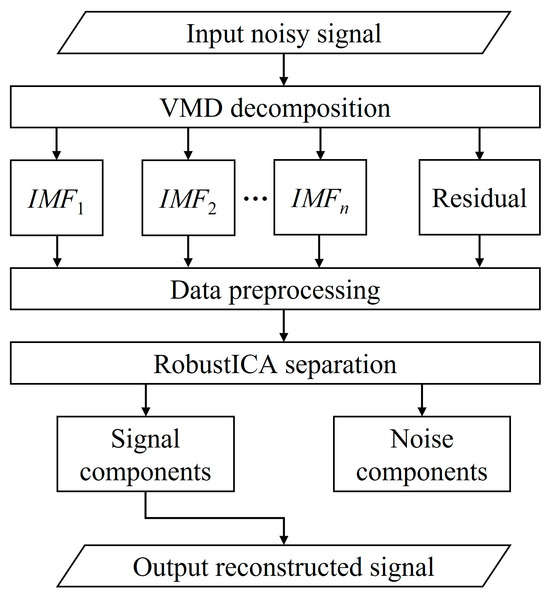
Figure 1.
Data processing workflow.
- Acquire MT signals contaminated with noise;
- Apply the VMD algorithm to decompose the MT signal into multiple IMFs;
- Use the IMFs obtained from VMD as inputs to the RobustICA algorithm for blind source separation, identifying and extracting independent signal sources;
- Evaluate the separated independent components, identify and suppress noise components, and recombine the useful signal components to reconstruct a denoised MT signal.
3. Simulation Experiments of Synthetic Signal
In the simulation experiments, a low-noise MT signal obtained from the measured station is considered as the high SNR original data. Non-stationary noise is then added to generate synthetic signals containing different types of noise. The performance of the VMD-RobustICA method under different values of K is compared with the denoising results obtained using VMD alone, validating the effectiveness of the proposed method and its robustness to manually selected parameters. To comprehensively evaluate the denoising performance of different methods on synthetic noisy data, we employ three metrics: the normalized cross-correlation coefficient (NCC), signal-to-noise ratio (SNR), and mean squared error (MSE) [38]:
where represents the original data, while denotes the denoised data. A higher SNR, an NCC value closer to 1, and a lower MSE indicate better denoising performance.
3.1. VMD Processing of Simulated Data Experiment
MT signals are typically non-stationary and nonlinear. During field data acquisition, they are often contaminated by noise with time-varying frequencies, random-walk noise, and intermittent high-frequency noise. These types of non-stationary noise usually exhibit large amplitudes and distinct characteristics, often completely overwhelming the MT signal in waveform plots. To analyze the decomposition performance of VMD on MT data containing different types of noise, we selected high-quality MT signals from an observation station located in a low-electromagnetic-noise environment as the original signals. We then simulated these typical types of noise for experimental analysis.
Figure 2 presents the time-domain waveforms of the original signal and those affected by chirp noise, random-walk noise, and intermittent high-frequency noise, which is designed based on the actual noise types observed in MT data. When these types of noise are added, their amplitudes significantly exceed that of the signal, completely masking the useful signal.
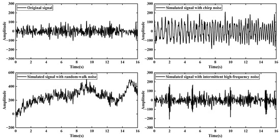
Figure 2.
Waveforms of original signal and simulated signal with noise.
Figure 3 illustrates the IMFs obtained through VMD decomposition of the three different types of noisy signals shown in Figure 2, with the number of modes K set to 5. In Figure 3a, VMD successfully distinguishes the overall shape of the chirp noise along with signal components of different central frequencies. Due to its high energy and prominent amplitude, the chirp noise constitutes the main component of the noise and can be identified as the noise part during signal reconstruction. In Figure 3b, the main components of random-walk noise are also effectively separated from the noisy signal using VMD. In Figure 3c, when processing impulse-like noise, mode mixing occurs between the signal and noise components, making it difficult to separate noise effectively from the corresponding frequency-band IMFs.
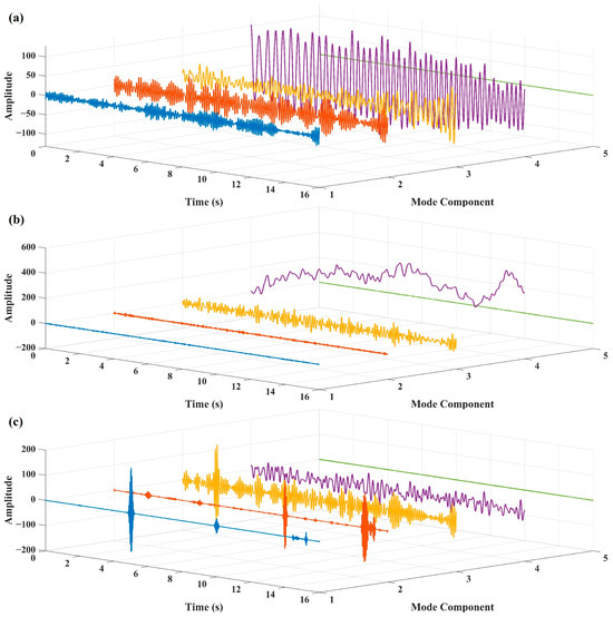
Figure 3.
Components of the VMD algorithm. The lines in different colors represent the modal components with different center frequencies: (a) signal with chirp noise; (b) signal with random-walk noise; and (c) signal with intermittent high-frequency noise.
It can be observed that, from the obtained IMF components, while VMD provides a rough distinction between noise and signal components, mode mixing still occurs in some cases. Additionally, since the decomposition performance of VMD is influenced by the manually set number of modes K, we assess the denoising performance under different K values using NCC, SNR, and MSE, as shown in Figure 4.
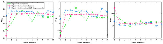
Figure 4.
NCC, SNR, and MSE under different K. The green curves are the results of signal with chirp noise. The red curves are the results of signal with random-walk noise. The blue curves are the results of signal with intermittent high-frequency noise.
We can see from Figure 4 that the quality of the reconstructed signal is highly dependent on the selected number of modes K. A low K value can cause mode mixing, where both signal and noise appear in the same component (e.g., chirp noise at K = 2 and K = 3), while an excessively high K may introduce mode redundancy, reducing reconstruction quality (e.g., impulse-like noise at K = 10). Optimal denoising occurs at K = 4 for chirp noise and K = 9 for impulse-like noise, achieving the highest NCC and SNR with the lowest MSE. In comparison, the removal of random-walk noise is more stable. Due to its dominant low-frequency components, it achieves consistently high NCC and SNR across a wide range of K values from 2 to 10.
As shown in Figure 5, the waveforms of the simulated noisy data and the signals obtained after performing VMD and reconstruction are displayed. It can be observed that the effective removal of the chirp noise and random-walk noise profiles was achieved. However, impulse-like noise remains, to some extent, in the reconstructed data. In Figure 5c, noticeable high-frequency disturbance components are present at approximately 2 s in the reconstructed signal. This is because the noise frequency in this region is close to the signal frequency, causing residual noise to remain in the IMF during the frequency band separation by VMD. Additionally, while the reconstructed signal in Figure 5a removes part of the chirp noise, this also leads to the loss of the MT signal in that frequency band. Therefore, the RobustICA algorithm is employed for further processing of the data in our study.
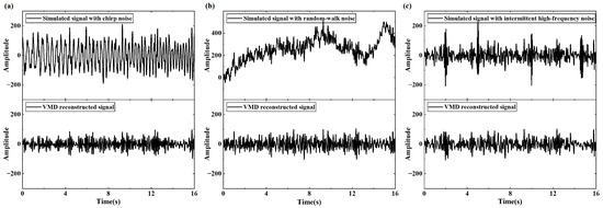
Figure 5.
Noisy signals and VMD reconstruction results: (a) signal with chirp noise; (b) signal with random-walk noise; and (c) signal with intermittent high-frequency noise.
3.2. RobustICA Processing of Simulated Data Experiment
In this section, the RobustICA algorithm is used to separate the independent components within the modal components, extracting the signal components from the noise while removing the residual noise from the VMD-reconstructed signals. Figure 6 shows the results of further separation using RobustICA on the VMD results, and compares them with the original low-noise signals. The results indicate that the reconstructed signal after RobustICA separation is very close to the original data in terms of the overall structure.
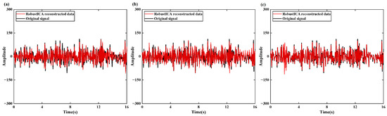
To quantitatively evaluate the denoising performance of VMD and VMD-RobustICA, Table 1 presents the quality evaluation parameters for the original signal and signals containing different noise using two methods. The results show that, across all evaluation metrics, the signal reconstructed after RobustICA separation is consistently superior to that obtained using VMD alone, with particularly notable improvements in SNR.

Table 1.
Quality evaluation parameters of Synthetic Signal Experiment.
4. Denoising of Simulated Data
To validate the reliability of the proposed denoising method, original MT signals with a relatively high SNR were collected from the field and then contaminated with artificially constructed non-stationary noise. Different types of noise were added to the original Hx and Hy signals, and their time-domain waveforms are shown in Figure 7 to evaluate the denoising performance of the proposed method.
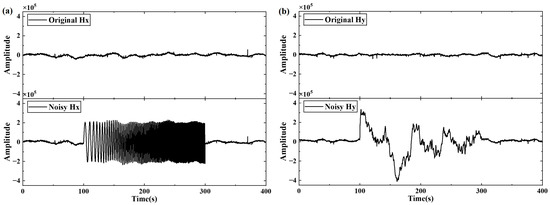
Figure 7.
Original signals and noisy data: (a) waveforms of original Hx and chirp noise added; and (b) waveforms of original Hy and random-walk noise added.
Figure 8 shows the time-domain waveforms of the noisy Hx and Hy signals before and after denoising using VMD and VMD-RobustICA methods. The results indicate that while VMD can effectively extract the noise profile of strong interference, it tends to lose some of the signal components in the corresponding noise frequency band. In particular, the loss of low-frequency components is more prominent in Figure 8b. However, after further extracting the independent components using RobustICA, the low-frequency signal profile can be partially recovered, improving the quality of the reconstructed signal and providing better denoising performance for different types and magnitudes of noise.
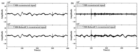
Figure 9 presents a comparison of the time–frequency spectra of the original signals before and after denoising. After adding strong non-stationary interference, the time–frequency spectra of both Hx and Hy signals show significant noise energy. The effective signal is largely masked, making it difficult to identify. When using the VMD method for decomposition and reconstruction, data within the entire noise frequency band can be removed. However, the proposed VMD-RobustICA method can further preserve some of the signal data from the noise profile, making the time–frequency spectrum characteristics of the denoised MT signal clearer, and the energy of the effective signal becomes more prominent.
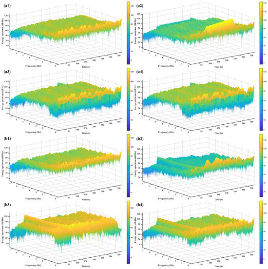
Figure 9.
Time–frequency spectra of MT data before and after denoising: (a1) original Hx; (a2) Hx with noise; (a3) reconstruction of Hx using VMD; (a4) reconstruction of Hx using VMD-RobustICA; (b1) original Hy; (b2) Hy with noise; (b3) reconstruction of Hy using VMD; and (b4) reconstruction of Hy using VMD-RobustICA.
To verify the effectiveness of the proposed method in processing MT signals, we compare the apparent resistivity-phase curves of the original, noisy, and denoised data. The processing workflow first uses SSMT2000 software (version 0.6.0.69) for time-series preprocessing, including Fourier transform and impedance tensor estimation. Since the software integrates a robust algorithm, it directly provides conventional robust impedance estimates for noisy data. For visualization and further optimization, we use MTeditor (version 0.99.2.106) to display the processing results. MTeditor applies an internal automatic calculation algorithm to perform unweighted averaging, which partially removes spurious jumps in the curves. Therefore, its automatic calculation results are regarded as an optimized version of the robust method, which is widely recognized as stable and reliable in practical engineering applications. In addition, to evaluate the suppression of non-stationary noise, we include two representative time–frequency analysis methods for comparison: wavelet transform, representing traditional time–frequency decomposition; and VMD, an emerging method that has recently attracted widespread attention.
In Figure 10, the apparent resistivity curve shows a slight shift, while the and phase curves , remain relatively stable. Under the influence of strong noise, the apparent resistivity and phase curves exhibit noticeable jumps. The Robust impedance estimation results obtained using SSMT2000 and MTeditor software show a significant improvement, but some jump points remain, especially near 0.005 Hz. When wavelet transform is applied for denoising, the performance improves slightly in the mid-frequency range; however, in the band of 0.1–0.5 Hz, the apparent resistivity curves still exhibit obvious jumps, and the phase response below 0.005 Hz shows no noticeable enhancement. In comparison, VMD effectively removes the noise profile from the data and smooths these curves to a great extent, but, due to the narrowband characteristics of the IMF components, it becomes difficult to distinguish between noise and a valid signal at extremely low frequencies, leading to significant deviations in the phase curve in that region. In contrast, the apparent resistivity-phase curves reconstructed using VMD-RobustICA are much smoother and more continuous, with jumping points almost completely eliminated. These curves are very close to the apparent resistivity-phase curves of the original low-noise signal, and the quality of the reconstructed signal is further improved, demonstrating the feasibility of the proposed method for denoising MT signals.
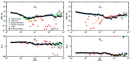
Figure 10.
Apparent resistivity-phase curves before and after denoising.
For the number of modes K in VMD, previous studies generally suggest that K = 5 is a reasonable default. In our synthetic data experiments, we evaluated the decomposition performance of VMD on chirp-like noise, random-walk noise, and impulse-like noise. Figure 4 shows the denoising results for typical non-stationary noise with K ranging from 1 to 10. Random-walk noise is relatively insensitive to K; impulse-like noise performs best at K = 5 or 6 but degrades noticeably at K = 7; and chirp-like noise shows better results at K = 4 or 5 but performs poorly at K = 2, 3, or 6. Overall, when noise is weak and the signal structure is simple, a smaller K can be chosen, whereas more complex data with richer frequency components require a slightly larger K. Miao et al. proposed an adaptive parameter selection method for VMD and found, in simulations, that their approach automatically converged to K = 5 for several synthetic signals [39]. Guo et al. reported that, for non-stationary MT signals, K around 4 provides a good representation of instantaneous spectral details, while K values exceeding 5 significantly increase errors, reducing the stability and convergence of impedance estimation [40]. Liu et al. selected K = 6 to balance the resolution and signal integrity based on multiple tests with synthetic and field data, but also noted that, for simpler synthetic signals, K = 4 or 5 achieves comparable decomposition performance [41]. Therefore, in our experiments, we adopt K = 5 as the number of VMD modes, as K = 4 or 6 produces no significant changes, while K = 3 (which may cause mode mixing) and K = 7 (which tends to introduce mode redundancy) are specifically analyzed for comparison.
Table 2 shows the denoising results of VMD and VMD-RobustICA under different K values. The results indicate that, except for the noisy Hx signal with K = 7, where the SNR of VMD-RobustICA is slightly lower than that of the VMD method, the proposed method is more effective in all other cases. Even when VMD fails to remove the noise profile due to mode mixing (for example, in the noisy Hx signal at K = 3), the noise profile can still be eliminated by evaluating its statistical independence, improving the quality of the reconstructed data. This demonstrates that the proposed method is robust to the influence of manually selected parameters.
Table 2.
Quality evaluation parameters of simulated experiment under different K.
Figure 11 presents the denoising results for different K values selected manually. It can be observed that the apparent resistivity and phase curves of the initial noisy data exhibit varying degrees of jumps over a wide frequency range (0.001–1 Hz). After VMD decomposition and reconstruction, the curve shapes become noticeably more regular and ordered. However, for K = 3, mode mixing causes the phase curve to show a decreasing trend in the 0.001–0.01 Hz range, which significantly deviates from the phase curve of the original data in that frequency band. After further using RobustICA, this error is improved. Similarly, for K = 7, due to mode redundancy, significant jumps appear in the extremely low-frequency part of , but, after applying RobustICA, the amplitude of these jumps is reduced, leading to better reconstruction quality.
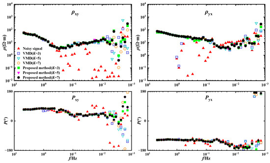
Figure 11.
The apparent resistivity and phase curves under different K values.
5. Denoising of Measured Data
This study utilizes measured MT data from the Balin Zuoqi area in Inner Mongolia. Focusing on the typical non-stationary noise in MT signals, the proposed VMD-RobustICA method is applied to the noisy data and compared with the built-in Robust method in the software of SSMT2000 and MTeditor, as well as with wavelet-transform-based and VMD-based denoising approaches. Figure 12 shows the time-domain waveforms of the electric and magnetic channel data at the site N2-22 before and after denoising. As this station is located near a mineralized area, the MT data are affected by strong interference. The Ex, Hx, and Hy channels all contain evident triangular wave-like noise, with the amplitude and frequency varying over time, causing noticeable distortion in the observed signal during those periods. Additionally, the Ey channel contains prominent charge–discharge noise, which causes significant distortions in the signal shape during certain periods. Furthermore, there are instantaneous jumps of impulse noise that almost cover the entire time period, affecting the entire frequency band of data processing. After denoising the time series using the proposed method, the trend of the effective signal is restored. All four electromagnetic channel signals show significant improvements in shape, with the smoothness of the time-domain waveforms greatly enhanced. Impulse spikes are largely eliminated, and the distortion caused by noise is effectively suppressed. To further evaluate the denoising effect, we use SSMT2000 to analyze the apparent resistivity and phase curves of the processed data.
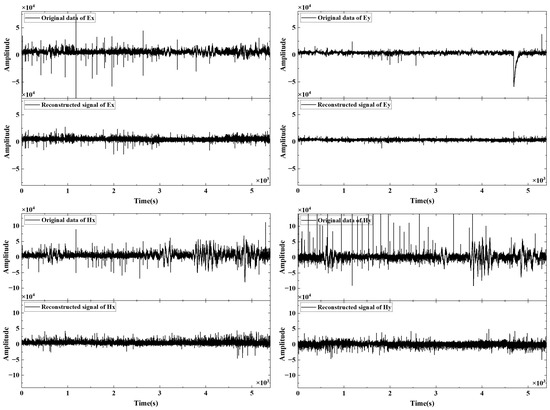
Figure 12.
Original signals and denoised waveforms.
Figure 13 presents a comparison of the apparent resistivity-phase curves in the low-frequency band at the site N2-22 before and after processing. Analyzing the apparent resistivity curves of the original data in Figure 13, it can be observed that, within the frequency range of 0.1 to 0.001 Hz, the curves exhibit poor overall continuity, instability, and a lack of smoothness. The corresponding phase curves are also severely distorted in this range, with approximately 10 data points completely deviating from the normal values. Due to the complex noise environment in the region and significant interference, the signal quality is poor with a low SNR, so that the application of the Robust method does not result in significant improvements to the curve. When wavelet transform is applied, noticeable jumps remain in the apparent resistivity curves within the 0.01–0.05 Hz band, indicating its limited denoising capability under strong noise conditions. After applying VMD processing to the measured data, the apparent resistivity shows some improvement, but the phase curve still exhibits considerable irregularities. In contrast, when we apply the VMD-RobustICA method proposed in this paper, both the apparent resistivity and phase curves show a certain degree of improvement, with fewer jump points present. However, due to the less distinct statistical characteristics of the modal components, the separation between signal and noise in the independent components is limited; thus, the apparent resistivity and phase curves have not achieved a stable convergence.
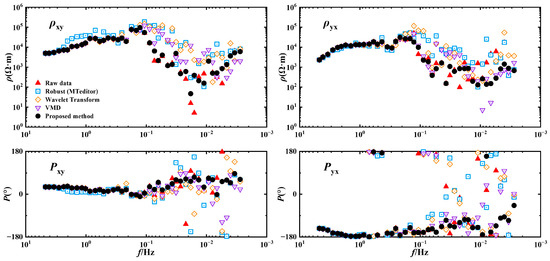
Figure 13.
Apparent resistivity and phase curves of site N2-22.
To determine the effectiveness of the VMD-RobustICA denoising method in practical applications, we use more MT data from additional sites (1545, 4567, 4568, and 1957), which are located in the Songliao Basin, a relatively noise-free area far from urban centers. Despite the generally low anthropogenic noise, any external interference leads to noticeable waveform distortions. In the apparent resistivity and phase curves of these fields, jumps appear only in certain frequency ranges. Figure 14 compares the proposed denoising method with the MTeditor software’s Robust estimation, the wavelet-transform-based method, and the VMD reconstruction approach. It can be observed that the results from MTeditor still show obvious jumps in the extremely low frequencies. VMD effectively improves the apparent resistivity-phase curves after separating the noise frequencies. In Figure 14b, the original signal shows significant noise around 0.1 Hz, which is notably improved after VMD processing. In Figure 14c, the low-frequency part below 0.01 Hz is also smoother than the original signal curve. However, in the 0.1 Hz to 1 Hz range, although there is some reduction in distortion compared to the original signal, several jumps remain, indicating that noise in this frequency range has not been effectively removed. In contrast, the wavelet-transform-based method shown in Figure 14d exhibits a resistivity trend that is clearly different from the other methods, suggesting that the selected wavelet basis may not be well-suited for this signal segment. By comparison, the proposed method results in a smoother apparent resistivity curve in this frequency range, with only one point showing a slight deviation. This improvement arises from RobustICA, which further extracts and suppresses the independent noise components from the IMF in this frequency band. The curves for the other stations also show improvements, with the apparent resistivity-phase curves restored to a smoother state, outperforming those obtained through VMD decomposition and reconstruction. Significant improvements are observed for most of the jumping points, making the curves more continuous. Although minor fluctuations remain at a few frequency points, their amplitudes are significantly reduced, demonstrating the reliability and effectiveness of the proposed denoising method. Figure 15 further presents the apparent resistivity-phase curves under different K values in the Songliao Basin, showing that the proposed method yields more robust response curves across different parameter settings.
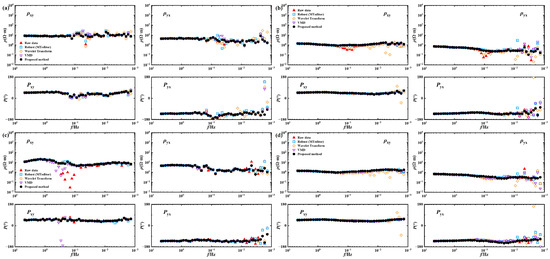
Figure 14.
Apparent resistivity-phase curves of more measured stations in Songliao Basin: (a) site 4567; (b) site 1545; (c) site 4568; and (d) site 1957.
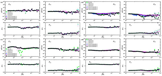
Figure 15.
Apparent resistivity-phase curves of more measured stations under different K values in Songliao Basin: (a) site 4567; (b) site 1545; (c) site 4568; and (d) site 1957.
6. Discussion
Geophysical exploration methods such as gravity, magnetics, electrical, seismic, and well logging extract subsurface structural information based on contrasts in the physical properties of geological bodies, providing critical references for mineral exploration [42]. Among these, the magnetotelluric sounding method has attracted widespread attention in the industry due to its large exploration depth range, low operational cost, and insensitivity to high-resistivity shielding. It has found important applications in deep mineral prospecting and hydrocarbon reservoir exploration [43,44]. However, the increasing severity of anthropogenic noise has significantly constrained the application of MT methods. In response, two main directions have emerged in previous research. On one hand, improved techniques with stronger anti-noise capabilities—such as controlled-source audio-frequency magnetotellurics (CSAMT) [45] and large-scale electromagnetic methods [46]—have been developed to partially replace MT in environments with strong electromagnetic interference, enabling deep exploration under challenging conditions. On the other hand, numerous noise suppression techniques for MT data have been proposed, including the remote reference method [47], robust impedance estimation [48], and bounded-influence remote reference processing (BIRRP) [49], aiming to mitigate the impact of anthropogenic noise on MT data quality. Nonetheless, improving MT exploration techniques is a long-term endeavor. Many new electromagnetic exploration methods enhance noise suppression at the cost of reduced exploration depth, making them suitable primarily for shallow investigations as a complement to conventional MT. Moreover, other geophysical methods often fail to achieve the same depth coverage with comparable cost-effectiveness in terms of time and labor. Therefore, research on MT data denoising remains crucial for advancing deep exploration efforts. One major challenge in MT denoising lies in the non-stationary nature of both the signal and noise. The time-varying spectral and statistical characteristics of MT data limit the effectiveness of frequency-domain-based suppression methods such as remote reference and robust techniques [50,51]. Furthermore, signal-decomposition-based MT processing methods, which have become increasingly popular in recent years, rely heavily on multiple parameter settings. In complex and highly variable field environments, the types, amplitudes, and durations of cultural noise near observation sites exhibit strong randomness, making it difficult to predefine optimal parameters based on experience. Improper parameter selection often results in residual noise or the loss of valid signals, leading to distortions in the apparent resistivity and phase curves. This raises higher demands for the self-adaptivity and parameter robustness of MT data-processing methods.
In order to deal with the non-stationary characteristics of MT signals and noise, the time–frequency analysis method is adopted in this study, and the signal decomposition technology is applied to preprocess MT data. VMD adaptively adjusts the instantaneous amplitude and frequency of each mode, providing fine time–frequency resolution that helps isolate transient, high-energy noise components. Meanwhile, although the spectrum of non-stationary noise varies over time, its higher-order statistical features remain distinct from those of the natural background field. RobustICA utilizes these differences by maximizing the statistical independence of modes, allowing it to remove residual noise without assuming stationarity. As a result, the combined approach is effective for processing non-stationary MT data. We evaluated the performance of VMD-RobustICA by comparing it with classical robust impedance estimation, wavelet transform, and VMD alone (Figure 10, Figure 13 and Figure 14). In the simulation experiments using two kinds of non-stationary noise (chirp-like noise and random-walk noise), this method successfully removes the strong interference in the interval of 100–300 s, while retaining the overall waveform of the original signal (Figure 8). The quality of low-frequency data was noticeably improved, with far fewer abrupt jumps in the apparent resistivity and phase curves (Figure 10). Compared with VMD alone, both NCC and SNR improved significantly (Table 2), with SNR gains of up to 15 dB and reduced MSE, indicating superior denoising performance under non-stationary noise. Similar improvements were observed across chirp-like, random-walk, and impulse-type noise scenarios. For field data from the Songliao Basin, where cultural noise is more evident (Figure 14), VMD-RobustICA produced results consistent with the simulations. Compared with MTeditor’s optimized robust processing, the apparent resistivity curves became more continuous in the 0.001–0.01 Hz range, with fewer spurious jumps. This shows that the method is more effective in suppressing strong cultural noise, short-term industrial interference, and transient disturbances, while retaining valid low-frequency information.
To address the strong parameter dependence in MT signal decomposition, this study combines adaptive signal decomposition with blind source separation. VMD is a fully adaptive method whose optimization objective is directly derived from the amplitude–frequency characteristics of the signal, without requiring predefined basis functions, making it well-suited to different noise types. Although VMD still requires specifying the number of modes K, the subsequent RobustICA step further processes the initial decomposition by separating statistically independent components, effectively resolving mode mixing. This significantly reduces the impact of an improper K value, so the final denoising result is no longer highly sensitive to manual parameter tuning. As a result, the method remains stable even in complex noise environments or when multiple noise types overlap. In simulation experiments, the denoising results obtained under different K values (Figure 11, Table 2) show that VMD alone is highly sensitive to parameter settings. When K is too small, severe mode-mixing occurs, with the NCC dropping to just 0.019, far below the optimal K result of 0.727. The apparent resistivity and phase curves exhibit prominent spikes near 1 Hz and discontinuities in the 0.001–0.01 Hz range, deviating significantly from the clean signal. In contrast, VMD-RobustICA maintains consistently high NCC values (0.665–0.746) across different K settings. The apparent resistivity curves show no obvious distortion around 1 Hz and remain continuous in the low-frequency range of 0.001–0.01 Hz, and the amplitude of phase jumps is greatly reduced. In measured data processing, similar results can also be observed (Figure 15). This demonstrates that the method retains good robustness under uncertain parameter settings, effectively mitigating the dependence of denoising performance on parameter selection.
However, for field data from the Balin Zuoqi mining area (Figure 13), the method is less effective. The improvements in the apparent resistivity and phase curves are clearly weaker than those in the synthetic experiments and at sites such as the Songliao Basin. This is mainly because the cultural noise in Balin Zuoqi has a low amplitude, long duration, and strong spectral overlap with the useful signal, making it difficult for VMD to distinguish noise from target signals based solely on time–frequency energy features. Moreover, the long-duration noise modes show significant differences in kurtosis, which prevents RobustICA from reliably separating independent source signals using kurtosis as a criterion. Since VMD-RobustICA relies on both energy concentration and statistical independence to identify noise, it struggles when the noise has a weak energy contrast and similar spectral and statistical properties to the signal. As a result, residual noise cannot be fully removed. In addition, noise in complex mining areas is often multi-sourced, and spatially correlated, and exhibits localized temporal patterns. The method only deals with single-channel data, without using joint analysis or external prior information across multiple sites, which further limits the adaptability in this case. Similar issues are also reported by Zhou et al. [52], whose method performs well on synthetic data and impulsive long-duration noise but still leaves low-amplitude residual noise in complex field recordings. In future work, we will address these challenges by integrating multi-channel or multi-site collaborative analysis and integrating additional statistical features, so as to enhance noise identification and improve the robustness of denoising in complex environments.
7. Conclusions
The magnetotelluric method in mineral exploration requires high-quality data. To remove noise from non-stationary MT signals, we propose a denoising method that combines VMD and RobustICA. VMD adaptively decomposes the signal into multiple modal components with clear physical meaning, effectively removing the noise component’s profile. RobustICA further distinguishes the independent components based on the statistical characteristics of the IMFs, extracting valid signals from the noise profiles and compensating for the decline in reconstructed signal quality caused by improperly set parameters in VMD. The effectiveness of this method in long-term noise identification and removal has been validated through simulations and field-data-processing results.
In the simulation experiments, our method is compared with the results from the MTeditor software’s Robust estimation, wavelet-transform-based denoising, and VMD processing. After denoising using the VMD-RobustICA method, the time-domain waveforms are closer to the original signal, and the information in the time–frequency spectrum is more complete. The denoising simulations for typical non-stationary noise show that this method achieves better data quality, effectively improves the signal-to-noise ratio, and is robust to user-defined parameters. Additionally, the processing results for field data from multiple regions indicate that, after applying the proposed method, the apparent resistivity-phase curves become smoother and more continuous.
This method has many advantages in processing low SNR MT data with non-stationary noise backgrounds, showing promising application potential in mineral exploration. Compared with traditional methods, it considers both the time–frequency spectrum information and statistical feature indicators of the signal, reducing the reliance on parameters and providing more robust denoising results. However, this method still has certain limitations. In practical exploration, many uncertainties exist, and the noise environment can be more complex. Since RobustICA is based on the assumption of independence from higher-order statistics, if the SNR is too low, leading to insufficient distinction in statistical features, or if the components obtained from VMD decomposition exhibit similar non-Gaussian characteristics, it may not accurately differentiate between noise and signal independent components. Furthermore, both VMD and RobustICA are cyclic iterative algorithms, resulting in low processing efficiency for large-scale MT signals obtained from long-term observations. Therefore, addressing these challenges to improve the practical applicability of this method in mineral exploration will be a key focus in our future research.
Author Contributions
Conceptualization, C.H. and Z.G.; methodology, C.H. and Z.G.; software, C.H.; validation, C.H. and Z.G.; formal analysis, C.H. and Z.G.; investigation, C.H.; resources, Z.G.; data curation, Z.G., C.H. and J.H.; writing—original draft preparation, C.H.; writing—review and editing, Z.G., W.J. and T.H.; visualization, C.H.; supervision, Z.G.; project administration, Z.G.; funding acquisition, Z.G. and J.H. All authors have read and agreed to the published version of the manuscript.
Funding
This research was funded by the project “Research on Mechanisms of Non-stationarity in Magnetotelluric Signals Based on Tensor Decomposition” (20103248088); the National Natural Science Foundation of China (42404152 and 42474109), and the Key Science & Technology Support Project of Ministry of Natural Resources of China (ZKKJ202419).
Data Availability Statement
The data presented in this study are available upon request from the corresponding author.
Conflicts of Interest
The authors declare no conflicts of interest.
References
- Zhdanov, M. Geophysical Electromagnetic Theory and Methods, 1st ed.; Elsevier: Amsterdam, The Netherlands, 2009. [Google Scholar]
- Booker, J.R. The Magnetotelluric Phase Tensor: A Critical Review. Surv. Geophys. 2013, 35, 7–40. [Google Scholar] [CrossRef]
- Chave, A.D.; Jones, A.G. The Magnetotelluric Method: Theory and Practice; Cambridge University Press: Cambridge, UK, 2012. [Google Scholar] [CrossRef]
- Yao, H.; Ren, Z.; Tang, J.; Guo, R.; Yan, J. Trans-dimensional Bayesian joint inversion of magnetotelluric and geomagnetic depth sounding responses to constrain mantle electrical discontinuities. Geophys. J. Int. 2023, 233, 1821–1846. [Google Scholar] [CrossRef]
- Chen, H.; Xie, X.; Liu, E.; Zhou, L.; Yan, L. Application of infrared remote sensing and magnetotelluric technology in geothermal resource exploration: A case study of the wuerhe area, Xinjiang. Remote Sens. 2021, 13, 4989. [Google Scholar] [CrossRef]
- Vargas, C.A.; Gomez, J.S.; Gomez, J.J.; Solano, J.M.; Caneva, A. Space–Time Variations of the Apparent Resistivity Associated with Seismic Activity by Using 1D-Magnetotelluric (MT) Data in the Central Part of Colombia (South America). Appl. Sci. 2023, 13, 1737. [Google Scholar] [CrossRef]
- Sims, W.E.; Bostick, F.X.; Smith, H.W. The estimation of magnetotelluric impedance tensor elements from measured data. Geophysics 1971, 36, 938–942. [Google Scholar] [CrossRef]
- Nabighian, M.N.; Grauch, V.; Hansen, R.; LaFehr, T.R.; Li, Y.; Peirce, J.W.; Phillips, J.; Ruder, M.E. The historical development of the magnetic method in exploration. Geophysics 2005, 70, 33ND–61ND. [Google Scholar] [CrossRef]
- Banks, R.J. The effects of non-stationary noise on electromagnetic response estimates. Geophys. J. Int. 1998, 135, 553–563. [Google Scholar] [CrossRef][Green Version]
- Weckmann, U.; Magunia, A.; Ritter, O. Effective noise separation for magnetotelluric single site data processing using a frequency domain selection scheme. Geophys. J. Int. 2005, 161, 635–652. [Google Scholar] [CrossRef]
- Xu, X.; Butala, M.D. Parametric magnetotelluric impedance tensor estimation. IEEE Trans. Geosci. Remote Sens. 2022, 60, 5910313. [Google Scholar] [CrossRef]
- Guo, R.; Dosso, S.E.; Liu, J.; Liu, Z.; Tong, X. Frequency-and spatial-correlated noise on layered magnetotelluric inversion. Geophys. J. Int. 2014, 199, 1205–1213. [Google Scholar] [CrossRef]
- Tikhonov, A.N. On determining electrical characteristics of the deep layers of the Earth’s crus. Dokl. Akad. Nauk. 1950, 73, 295–297. [Google Scholar]
- Cagniard, L. Basic theory of the magnetotelluric method of geophysical prospecting. Geophysics 1953, 18, 605–635. [Google Scholar] [CrossRef]
- Goubau, W.M.; Gamble, T.D.; Clarke, J. Magnetotelluric data analysis: Removal of bias. Geophysics 1978, 43, 1157–1166. [Google Scholar] [CrossRef]
- Gamble, T.D.; Goubau, W.M.; Clarke, J. Magnetotellurics with a remote magnetic reference. Geophysics 1979, 44, 53–68. [Google Scholar] [CrossRef]
- Egbert, G.D.; Booker, J.R. Robust estimation of geomagnetic transfer functions. Geophys. J. Int. 1986, 87, 173–194. [Google Scholar] [CrossRef]
- Chave, A.D.; Thomson, D.J. Some comments on magnetotelluric response function estimation. J. Geophys. Res. Solid Earth 1989, 94, 14215–14225. [Google Scholar] [CrossRef]
- Wang, S.; Wang, J. Application of Higher-Order Statistics in Magnetotelluric Data Processing. Chin. J. Geophys. 2004, 47, 1046–1053. [Google Scholar] [CrossRef]
- Zhou, C.; Tang, J.; Yuan, Y.; Deng, J.; Shi, F.; Li, Y. Magnetotelluric multi-reference array data processing algorithm. In Proceedings of the 9th International Conference on Environmental and Engineering Geophysics, Changchun, China, 11–14 October 2020. [Google Scholar] [CrossRef]
- Chave, A.D. Estimation of the magnetotelluric response function. the path from robust estimation to a stable maximum likelihood estimator. Surv. Geophys. 2017, 38, 837–867. [Google Scholar] [CrossRef]
- Neukirch, M.; Garcia, X. Nonstationary magnetotelluric data processing with instantaneous parameter. J. Geophys. Res. Solid Earth 2014, 119, 1634–1654. [Google Scholar] [CrossRef]
- Guo, Z.; Gong, X.; Han, J.; Liu, L.; Wu, Y.; Meng, F.; Kang, J. Research on a multiscale denoising method for low signal-to-noise magnetotelluric signal. IEEE Trans. Geosci. Remote Sens. 2022, 60, 5925018. [Google Scholar] [CrossRef]
- Chant, I.J.; Hastie, L.M. Time-frequency analysis of magnetotelluric data. Geophys. J. Int. 1992, 111, 399–413. [Google Scholar] [CrossRef]
- Trad, D.O.; Travassos, J.M. Wavelet filtering of magnetotelluric data. Geophysics 2000, 65, 482–491. [Google Scholar] [CrossRef]
- Zhan, Q.; Liu, Y.; Liu, C.; Zhao, P. A novel decomposition-enhanced denoising method for magnetotelluric data based on AMSE-REWT in the time-frequency domain. IEEE Trans. Geosci. Remote Sens. 2025, 63, 5906312. [Google Scholar] [CrossRef]
- Cai, J. A de-noising method of magnetotelluric signals based on the generalized S-transform. J. Appl. Geophys. 2024, 223, 105349. [Google Scholar] [CrossRef]
- Huang, N.E.; Wu, Z. A review on Hilbert-Huang transform: Method and its applications to geophysical studies. Rev. Geophys. 2008, 46, RG2006. [Google Scholar] [CrossRef]
- Li, J.; Ma, F.; Tang, J.; Liu, Y.; Cai, J. Denoising application of magnetotelluric low-frequency signal processing. IEEE Trans. Geosci. Remote Sens. 2022, 60, 5920518. [Google Scholar] [CrossRef]
- Dragomiretskiy, K.; Zosso, D. Variational mode decomposition. IEEE Trans. Signal Process. 2014, 62, 531–544. [Google Scholar] [CrossRef]
- Zhang, L.; Tang, J.; Li, G.; Chen, W. Audio magnetotelluric denoising via variational mode decomposition and adaptive dictionary learning. J. Appl. Geophys. 2022, 204, 104748. [Google Scholar] [CrossRef]
- Cai, L.F.; Tian, X.M. A new fault detection method for non-Gaussian process based on robust independent component analysis. Process Saf. Environ. Prot. 2014, 92, 645–658. [Google Scholar] [CrossRef]
- Yao, J.; Xiang, Y.; Qian, S.; Wang, S.; Wu, S. Noise source identification of diesel engine based on variational mode decomposition and robust independent component analysis. Appl. Acoust. 2017, 116, 184–194. [Google Scholar] [CrossRef]
- Tharwat, A. Independent component analysis: An introduction. Appl. Comput. Inform. 2020, 17, 222–249. [Google Scholar] [CrossRef]
- Wang, S.; Wang, J. Analysis on statistic characteristics of magnetotelluric signal. Acta Seism. Sin. 2004, 17, 735–740. [Google Scholar] [CrossRef]
- Cao, X.; Jiang, T. Suppression method of MT interference noise based on marginal spectrum and blind source separation. In Proceedings of the 2023 IEEE International Conference on Control, Electronics and Computer Technology, Jilin, China, 28–30 April 2023. [Google Scholar] [CrossRef]
- Zarzoso, V.; Comon, P. Robust independent component analysis by iterative maximization of the kurtosis contrast with algebraic optimal step size. IEEE Trans. Neural Netw. 2010, 21, 248–261. [Google Scholar] [CrossRef]
- Li, G.; He, Z.; Deng, J.; Tang, J.; Fu, Y.; Liu, X.; Shen, C. Robust CSEM data processing by unsupervised machine learning. J. Appl. Geophys. 2021, 186, 104262. [Google Scholar] [CrossRef]
- Miao, Y.; Zhao, M.; Lin, J. Identification of mechanical compound-fault based on the improved parameter-adaptive variational mode decomposition. ISA Trans. 2019, 84, 82–95. [Google Scholar] [CrossRef] [PubMed]
- Guo, Z.; Han, J.; Liu, L.; Wu, Y.; Hou, J.; Gong, X. Reducing Reliance on Observation Duration of Magnetotelluric Impedance Estimation with an Improved Instantaneous Spectrum-Based Method. IEEE Trans. Geosci. Remote Sens. 2024, 62, 5912715. [Google Scholar] [CrossRef]
- Liu, Y.; Yang, G.; Li, M.; Yin, H. Variational mode decomposition denoising combined the detrended fluctuation analysis. Signal Process. 2016, 125, 349–364. [Google Scholar] [CrossRef]
- Oldenburg, D.W.; Li, Y.; Farquharson, C.G.; Kowalczyk, P.; Aravanis, T.; King, A.; Zhang, P.; Watts, A. Applications of geophysical inversions in mineral exploration. Lead. Edge 1998, 17, 461–465. [Google Scholar] [CrossRef]
- Varentsov, I.M.; Kulikov, V.A.; Yakovlev, A.G.; Yakovlev, D.V. Possibilities of magnetotelluric methods in geophysical exploration for ore minerals. Izv. Phys. Solid Earth 2013, 49, 309–328. [Google Scholar] [CrossRef]
- Jiang, W.; Duan, J.; Doublier, M.; Clark, A.; Schofield, A.; Brodie, R.C.; Goodwin, J. Application of multiscale magnetotelluric data to mineral exploration: An example from the east Tennant region, Northern Australia. Geophys. J. Int. 2022, 229, 1628–1645. [Google Scholar] [CrossRef] [PubMed]
- Zhang, L.; Li, G.; Chen, H.; Tang, J.; Yang, G.; Yu, M.; Hu, Y.; Xu, J.; Sun, J. Identification and Suppression of Multicomponent Noise in Audio Magnetotelluric Data Based on Convolutional Block Attention Module. IEEE Trans. Geosci. Remote Sens. 2024, 62, 5905515. [Google Scholar] [CrossRef]
- Mörbe, W.; Yogeshwar, P.; Tezkan, B.; Kotowski, P.; Thiede, A.; Steuer, A.; Rochlitz, R.; Günther, T.; Brauch, K.; Becken, M. Large-scale 3D inversion of semi-airborne electromagnetic data—Topography and induced polarization effects in a graphite exploration scenario. Geophysics 2024, 89, B339–B352. [Google Scholar] [CrossRef]
- Ritter, O.; Junge, A.; Dawes, G.J.K. New equipment and processing for magnetotelluric remote reference observations. Geophys. J. Int. 1998, 132, 535–548. [Google Scholar] [CrossRef]
- Sutarno, D.; Vozoff, K. Robust M-estimation of magnetotelluric impedance tensors. Explor. Geophys. 1989, 20, 383–398. [Google Scholar] [CrossRef]
- Chave, A.D.; Thomson, D.J. Bounded influence magnetotelluric response function estimation. Geophys. J. Int. 2004, 157, 988–1006. [Google Scholar] [CrossRef]
- Li, G.; Gu, X.; Chen, C.; Zhou, C.; Xiao, D.; Wan, W.; Cai, H. Low-Frequency Magnetotelluric Data Denoising Using Improved Denoising Convolutional Neural Network and Gated Recurrent Unit. IEEE Trans. Geosci. Remote Sens. 2024, 62, 5909216. [Google Scholar] [CrossRef]
- Li, G.; Liu, X.; Tang, J.; Deng, J.; Hu, S.; Zhou, C.; Chen, C.; Tang, W. Improved shift-invariant sparse coding for noise attenuation of magnetotelluric data. Earth Planets Space 2020, 72, 45. [Google Scholar] [CrossRef]
- Zhou, R.; Li, T.; Han, J.; Liu, L.; Guo, Z. Research on magnetotelluric long-duration noise reduction based on adaptive sparse representation. IEEE Trans. Geosci. Remote Sens. 2022, 60, 5925113. [Google Scholar] [CrossRef]
Disclaimer/Publisher’s Note: The statements, opinions and data contained in all publications are solely those of the individual author(s) and contributor(s) and not of MDPI and/or the editor(s). MDPI and/or the editor(s) disclaim responsibility for any injury to people or property resulting from any ideas, methods, instructions or products referred to in the content. |
© 2025 by the authors. Licensee MDPI, Basel, Switzerland. This article is an open access article distributed under the terms and conditions of the Creative Commons Attribution (CC BY) license (https://creativecommons.org/licenses/by/4.0/).